DEPARTMENT OF ECONOMICS

ARE AMERICANS MORE GUNG-HO THAN

EUROPEANS?

SOME EVIDENCE FROM TOURISM IN ISRAEL

DURING THE INTIFADA

David Fielding, University of Otago, New Zealand

Anja Shortland, University of Leicester, UK

Working Paper No. 04/29 December 2004

ARE AMERICANS MORE GUNG-HO THAN

EUROPEANS? EVIDENCE FROM TOURISM IN

ISRAEL DURING THE INTIFADA§

David Fielding and Anja Shortland,

January 2005

Abstract

Analysis of cross-sectional data on tourism to Israel during the Intifada

reveals some factors driving international tourist behaviour. Much of

the heterogeneity in the observed response of different nationalities can

be explained by socio-economic characteristics, some of which suggest

differences in attitudes towards the risk associated with violence in

Israel. Analysis of time-series data reveals the importance of different

dimensions of violence in explaining tourism decline, distinguishing

between violence affecting perceptions of risk and violence that might

influence tourists with strong political views. We also see why

variations in conflict intensity are more important than variations in

road accidents.

JEL classification: Z19, L83

- 1 -

I. Introduction

Recent years have seen the establishment of an economic literature (a large part of which is

reviewed by Frey et al., 2004) devoted to the consequences of violent conflict. Such violence

will impact on economic decisions to the extent that it affects people’s perceptions about the

relative risks involved in different activities. One decision in which such risks are most evident

is the choice of where to go on vacation. Several important international tourist destinations,

including Israel and the Palestinian Territories, are now severely affected by political violence.

There is an increasing body of evidence to suggest that violent incidents resulting in only a

handful of fatalities per year – and therefore representing only a very small risk to an individual

tourist – have a substantial impact on tourist volumes and tourism revenues. As pointed out by

Cukierman [2004], the economic effects of a small increase in the current level of violence can

be magnified when it raises the perceived probability of a substantial escalation of the conflict.1

Evidence for such effects in relation to tourism is reported in Enders and Sandler [1991]

(Spain), Enders et al. [1992] (Austria, Italy and Greece), Drakos and Kutan [2003] (Greece,

Israel and Turkey) and Sloboda [2003] (USA). Anecdotal evidence suggests that the effects of

violence on tourism are equally large in developing country destinations such as Bali and

Egypt.

Whatever the true nature of the risk, many OECD governments actively dissuade their

nationals from travelling to Israel. The following quotation from the US State Department

website (August 3, 2004) is typical of advice given to Western tourists:

'The Department of State warns US citizens to… defer travel to Israel, the West Bank and Gaza

due to current safety and security concerns.'

Such violence has serious economic repercussions for a tourism destination like Israel, where

since September 2000 there has been a marked increase in violent conflict between Israeli and

Palestinian forces (the Al-Aqsa Intifada). Tourist arrivals are now less than half their pre-2000

level, and between 1999 and 2003 annual tourism revenue fell from $4.3bn to $2.3bn. This fall

is almost equal in magnitude to the decline in the Israeli Balance of Payments in the same

period, from a $0.9bn surplus to a $1.3bn deficit.

It is not so surprising that the upsurge in violent conflict led to a dramatic fall in the

number of tourists in Israel. However, this simple statistic leaves many questions unanswered.

Many people have chosen not to visit Israel any more, but a substantial minority has been

undeterred by the violence. In this paper we will use time-series and cross-sectional data on

- 2 -

tourism in Israel to explore the characteristics of these two groups of people. Along the way we

will find out which dimensions of the violence affect tourists’ choices, and whether variations

in conflict intensity have more impact than variations the frequency of road traffic accidents.

We will also explore the factors that drive the differences we will observe in the behaviour of

tourists from different parts of the world. For example, some commentators insist that there are

still large cultural differences between Americans and Europeans with respect to risk-taking. In

the recent words of one Whitehouse spokesperson: 2

'An American personality… prizes the calculated risk… Europeans often seem bent on

preventing any chance of trouble arising.'

If this is so, then ceteris paribus we should observe Americans to be less deterred than

Europeans by the dangers of international tourism, and more inclined to ignore the advice of

the State Department.

Before we discuss our data and our model, the next section of the paper outlines in

more detail the conceptual framework for the paper.

II. A Conceptual Framework

In this paper we will use two slightly different Israeli datasets to address two key questions

about the behaviour of tourists.

1. First of all, we can ask a question about the distribution of attitudes towards the risk of death

or injury faced by travellers. The fact that some – but not all – tourists are staying away from

Israel these days suggests heterogeneous attitudes towards risk among the tourist population.

For some – but not all – tourists the higher risk appears to have raised the opportunity cost of

travelling to Israel above the benefit. The fall in tourist numbers is consistent with the

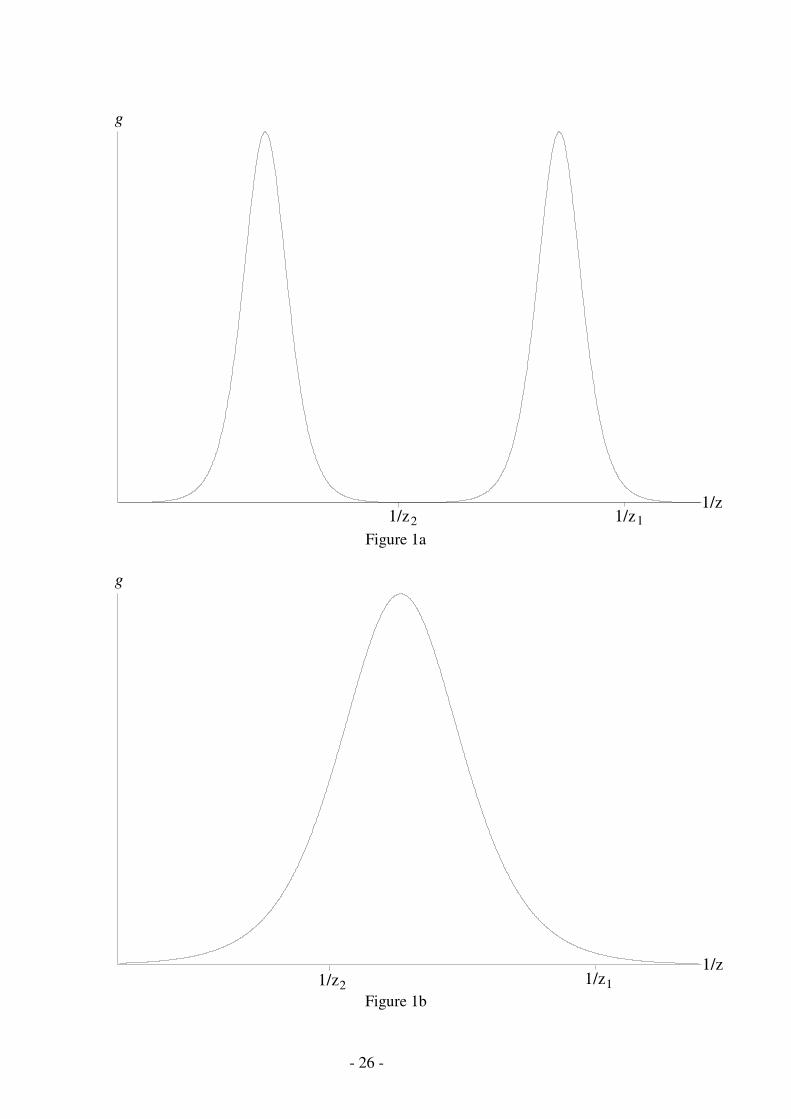
existence of discrete groups of people with different attitudes towards risk. Figure 1a illustrates

this case. (Figure 1 represents a rough sketch of a model that will be outlined in much greater

detail in section 3 below.) The frequency distribution in the figure indicates the number of

people, g, who are just indifferent between travelling and not travelling at a certain level of

risk, z. (Because the number of tourists is declining in the level of risk, we draw g as a function

of 1/z.) The fact that g is bimodal reflects the existence of two groups of people, a 'timid' group

clustered around the right-hand mode, and a 'gung-ho' group clustered around the left-hand

mode. The number of tourists will be the integral of g up to the current level of 1/z. As the risk

level rises from z1 to z2 between September and October 2000, the timid group drops out of the

- 3 -

travelling population. Subsequently, small variations in the level of risk around z2 have little or

no impact on tourist numbers. However, the fall in tourist numbers is also consistent with a

unimodal distribution, as illustrated in Figure 1b. In this case, there are no identifiable clusters

with respect to attitudes towards risk. The rise in risk from z1 to z2 again leads to a substantial

reduction in tourist numbers, but in this case subsequent variations around z2 do have a

substantial impact on tourist numbers.

[Figure 1 here]

Why does this matter? One reason is that the shape of g around z2 affects the return to marginal

improvements in the Israeli-Palestinian peace process. In Figure 1a nothing short of a complete

return to peace will have any substantial impact on tourist numbers. Piecemeal measures that

result in a partial reduction in violence cannot realistically be sold to the Israeli or Palestinian

public on economic grounds. This makes a gradual return to normality very difficult. By

contrast, in Figure 1b even a small reduction in violence yields an economic return, making

partial peace agreements easier to sell to the public, and facilitating a gradual return to peace.

2. The second question relates to differences in the attitudes of tourists of different

nationalities. The distributions in Figure 1 might vary from one part of the world to another,

because of variations in the (net) benefits to the average tourist from visiting Israel, or because

of variations in the costs associated with a certain level of risk. For example, the benefits might

be higher in countries with a large Jewish population. The costs associated with risk might be

lower in countries where people have learned better how to manage risk, or else have become

acclimatised to it. People in some places might just be more gung-ho than people elsewhere. If

there is cross-country variation in the size of the integral of g between z1 and z2, then an

increase in violence will have markedly different effects on tourist numbers from different

parts of the world.

If we can find correlates of the national characteristics that affect the shape of g, then

we will be able to explain at least some of the cross-country variation in the decline in tourist

numbers. As Table V below indicates, this variation has been substantial. This will provide

evidence on some of the ways in which national characteristics affect attitudes towards risk and

security.

In order to address the issues raised in the first question, we need to look at tourists’ response

to changes in the level of violence in Israel after September 2000, to see whether the relatively

small fluctuations in conflict intensity during the Intifada have been associated with changes in

- 4 -

tourist volumes. This requires the analysis of time-series data on tourist traffic. The Israeli

Central Bureau of Statistics (CBS) reports consistent monthly data on the number of American

tourists and on the number of European tourists checking into Israeli hotels each month. (Data

on tourist numbers in the West Bank and Gaza, virtually zero since September 2000, are not

included.) In the next section, we will outline a time-series model that is designed to explain

variations in these data. If the month-on-month variations in tourist volumes in response to

fluctuations in conflict intensity are substantial, relative to the large decline in tourism as a

result of the start of the Intifada, then we are likely to be in the world of Figure 1b rather than

that of Figure 1a. Small steps towards peace will yield an economic return, making a gradual

return to normality more likely. As part of this exercise, we will make a careful distinction

between those dimensions of the conflict that are associated with the direct risk to tourists and

other dimensions that might have an impact because of tourists’ political views.

The hotels data are not well suited to answering the second question, because they

disaggregate only between Americans, Europeans, and others. However, there are also annual

CBS data on tourist arrivals into Israel, disaggregated by the nationality of the individual

tourists. These data are not reported at a high enough frequency for time-series analysis, but we

can construct a cross-section in which the dependent variable is the rate of decline in tourist

arrivals from each country between 1998-9 (i.e., before the start of the Intifada) and 2001-2.3

We can then look at the national characteristics associated with cross-sectional variations in the

rate of decline.

Section 3 below first outlines the modelling framework used to analyse the time-series

data, then presents the results of our analysis. Section 4 deals similarly with the international

cross-sectional data.

III. The Time-series Model

3.1 The time-series data: concepts

Our time-series regression equations ought to be consistent with a plausible model of

individual decision-making. In this section we expand on the ideas outlined in section 2,

deriving a regression equation from the discrete choice theory outlined inter alia in Maddala

[1983].4

The model concerns a population of people who have already decided to take a

vacation, and are deciding where to go. Let the net utility an individual i derives from taking a

vacation in location m ∈ {1,..., M} in month t be designated vimt. We will assume that each

person’s utility is of the form:

- 5 -

vimt = µmt (Xmt, εmt) + uimt (1) where µmt is the average level of utility from visiting location m in month t for the vacationing

population and uimt is an individual’s idiosyncratic deviation from this average. Xmt is a vector

of identifiable time-varying factors that impact on one’s net utility from a vacation in a

particular location, and εmt is a stochastic term reflecting the unpredictable component of the

average utility level (fads and fashions). We further assume that individual i chooses location

m in period t if and only if:

vimt = max (vi1t,..., viMt) (2) It can be shown (Maddala, 1983) that if for any two locations (m, n) the distribution of uimt is

independent of that of uint, and if each has a Weibull distribution, then the probability of any

one randomly selected individual choosing location m in period t is:

∑ =

=

= Mj

j jt

mtimtp

1)exp(

)exp(µ

µ (3)

or, in logarithmic form:

∑ =

=−= Mj

j jtmtimtp1

)exp(ln)ln( µµ (4)

(If the only factor influencing the µ ’s were the level of risk, zmt, associated with travel to

location m, then our model would be as simple as the one depicted in Figure 1, with gmt =

dpimt/d(1/zmt). However, our model will not be so restrictive.) For a large population, the ratio

of the number of people in period t visiting location m (pmt) to the number visiting location n

(pnt) can therefore be written as:

pmt / pnt = exp(µmt) / exp(µnt) (5) and hence: ln(pmt) – ln(pnt) = µmt (Xmt, εmt) – µnt (Xnt, εnt) (6) Location m here is to be interpreted as Israel; the identity of the reference location n will be

discussed later. If we know the functional forms of µmt (.) and µnt (.), then we can fit equation

(6) to time-series data. In what follows, we assume that for the data after September 2000 it is

possible to find a linear specification such that:

- 6 -

ln(pmt) – ln(pnt) = [Xmt – Xnt]′β + εt (7) where εt is a linear function of εmt and εnt. Note that we are not assuming linearity across the

large change in conflict intensity following the onset of the Intifada, only linearity in the

smaller changes observed since.

We will begin with the assumption that [Xmt – Xnt] had four major components. The

first three are: seasonal factors, the anticipated relative enjoyability of the two locations and the

relative chances of being a victim of a violent incident in the two locations in this month and

the next. (Some tourist visits span two calendar months.) The fourth component relates to the

intensity of those elements of the conflict not associated with a direct risk to tourists. This

might be important if some pro-Palestinian tourists disapprove of Israeli occupation of the

West Bank, and if the intensity of their disapproval varies with the intensity of the conflict.5

(At the opposite end of the political spectrum, an increase in attacks on Israelis could stimulate

more pro-Israel “solidarity” tourism. We deal with this possibility by appropriate definition of

our dependent variable, as discussed in the next section.) Our regressions are based on an

equation of the form:

ln(pmt) – ln(pnt) = Σsθs.hst + β1.E[ln(wmt) – ln(wnt)] (8)

+ β3.E[ln(zmt+1) – ln(znt+1)] + β4.[ln(zmt) – ln(znt)]

+ β5.E[ln(fmt+1) – ln(fnt+1)] + β6.[ln(fmt) – ln(fnt)] + εt

hst is a dummy for month s. wmt is the enjoyability of location m in period t, to which an

expectations operator is attached, because new visitors will only find out whether they like a

place when they get there. zmt is the probability of being a victim of a violent incident and fmt is

a measure of conflict intensity not associated with risk to tourists. Terms in zmt+1 and fmt+1 are

included, because some visits may straddle two calendar months.6

One might also wonder whether monthly variations in the relative cost of different

locations make a difference to tourist numbers. However, as discussed in Appendix 1, our

empirical measures of relative cost were never statistically significant in any regression

equation. It seems that between 2000 and 2003, monthly variations in cost had no substantial

impact on tourism to Israel.

Application of the model requires us to specify the expectations formation process. We

will work with the following assumptions:

E[ln(wmt) – ln(wnt)] = α1(L)[ln(pmt-1) – ln(pnt-1)] (9a)

E[ln(zmt) – ln(znt)] = α2(L)[ln(zmt-1) – ln(znt-1)] (9b)

- 7 -

E[ln(fmt) – ln(fnt)] = α3(L)[ln(fmt-1) – ln(fnt-1)] (9c)

where the α(L)s are lag polynomial operators. Equation (9a) builds some herding behavior into

the model: if a destination has been popular in the past, people are more likely to consider it

today.7 Equation (9b) states that expectations about the current risk of violence are based on the

past frequency of similar violent incidents. Equation (9c) specifies a corresponding equation

for violence not associated with tourist risk. Substituting equations (9a)-9(b) into equation (8),

we will have an ARDL equation of the form:

γ1(L)[ln(pmt) – ln(pnt)] = Σsθs.hst + γ2(L)[ln(zmt) – ln(znt)] + γ3(L)[ln(fmt) – ln(fnt)] + εt (10)

where the γ(L)s are linear combinations of the α(L)s and the β ’s.

It is worth reiterating that the γ2 and γ3 parameters in equation (10) will be statistically

significant only if in-sample variations in the level of violence are making the difference to the

vacation location decisions of a substantial number of tourists. This will be the case as long as

there are a substantial number of people who are roughly indifferent between locations at the

average level of violence during the Intifada period. An obvious alternative to equation (10) –

though not one grounded so well in theory – is a regression equation for ln(pmt) alone rather

than [ln(pmt) – ln(pnt)]. The stylized facts reported in the next section are also true of regression

equations of this kind; however, such regressions do not fit the data so well.

3.2 The time-series data: application

We first discuss the measurement of the variables in equation (10). The equation is to be fitted

to the monthly hotels data for two tourist populations: tourists from America and tourists from

Europe. In order to estimate the parameters of the equation, we need to construct a dependent

variable in which the number of visitors to Israel from a certain population (America, Europe)

is expressed relative to the number of visitors from that population to other locations. In order

to focus on the effects of political violence within Israel, it will be convenient to use reference

locations that are reasonably safe. In the case of American tourists the reference location will

be Europe,8 and in the case of Europeans it will be America. That is, for the American tourist

sample, pmt is interpreted as the number of American visitors to Israel in a particular month and

pnt is interpreted as the number of American visitors to Europe. For the European tourist

sample, pmt is interpreted as the number of European visitors to Israel in a particular month and

pnt is interpreted as the number of European visitors to America.

- 8 -

For both samples, the monthly transatlantic tourism figures used to measure pnt are

taken from the dataset published by the ITA Office of Tourism and Travel Industries

(http://tinet.ita.doc.gov), which reports both American tourists departing to Europe and

European tourists arriving in America. The monthly Israeli tourism data are published by the

Central Bureau of Statistics and are available online at http://www.cbs.gov.il. The Israeli

tourism statistics used to measure pmt are those for American and European tourists checking

into tourist hotels. One advantage of using hotels data is that organised “solidarity” visits to

Israel make use mainly of accommodation in Israeli homes, rather than standard tourist hotels.

So we avoid some downward bias in the absolute value of the γ2 parameter due to solidarity

visits increasing at times of high violence.

Measures of zmt and fmt are constructed from data provided by the Israeli NGO

B'Tselem (http://www.btselem.org). Among other Intifada-related data, B'Tselem records: (i)

the total number of Israeli fatalities within Israel proper, excluding the West Bank and Gaza

(WBG); (ii) the total number of Israeli and Palestinian fatalities in WBG. The first of these

series is used as a measure of zmt. All – or almost all – fatalities within Israel proper, most of

which are from bomb attacks, are in situations in which tourists are just as likely to be victims

as Israeli residents. Of course, the vast majority of victims are Israelis, because the resident

population is so much larger than the tourist population. The second series is used as a measure

of fmt. Violence in WBG does not pose a direct risk to tourists to Israel, who don't have to go

there, but liberal-minded tourists might choose not to visit Israel because they lay part of the

blame for the violence on the Israeli government. It is worth noting at this point that

disaggregation of WBG fatalities by nationality and by combatant status has no extra

explanatory power in the regression equations reported in the next section.

In addition to the fatality series in Israel, we will include a dummy variable (DGW) for

the month of the Iraq War (2003m3). American and European tourists are likely to have

thought travel in the Mid East to be more risky during the war, or at least during the first

couple of weeks. The use of dummy variables in time-series regressions is never ideal: the

interpretation of dummy coefficients is always open to question. But we have no other way of

capturing the effect of the Gulf War, and removing the dummy from the regression does not

substantially alter our estimated long-run elasticities.9

In all cases we assume that znt = fnt = 0: there is no political violence in Europe or

America. Our sample period does encompass September 2001; but the attacks in America

made all overseas air travel more daunting for Americans, regardless of their destination. It

also seems to have been perceived in Europe as increasing the risk of air travel generally,

- 9 -

rather than air travel specifically to America. In any case, a dummy variable for 2001m9 is not

statistically significant in the regression equations reported below.

Figures 2-3 depict the time-series [ln(pmt) – ln(pnt)], ln(zmt) and ln(fmt) in each of our two

samples. Table I provides some descriptive statistics for the variables for our sample period

(2000m9-2004m2, or 42 observations), as well as for the period before the onset of the

Intifada. The table shows how much the mean values of both tourism and conflict intensity

have changed: the Intifada represents a large structural break. As in many other empirical

applications, it is unclear whether the variables are I(0) or I(1) over the 2000m9-2004m2

sample period: standard tests reject neither null at conventional levels of significance. So it is

appropriate to re-parameterize equation (10) in error-correction form. Employing such a re-

parameterization of equation (10) with the restriction that znt = fnt = 0, and also allowing for the

Gulf War dummy, we have:

η1(L)∆[ln(pmt) – ln(pnt)] = Σsθs.hst + η2(L)∆ln(zmt) + η3(L)∆ln(fmt) (11)

+ ϕ1.[ln(pmt-1) – ln(pnt-1)]+ ϕ2.ln(zmt-1) + ϕ3.ln(fmt-1) + δ.DGWt + εt

where the ϕ ’s capture the long-run levels relationship between the variables.10 In both the

American and the European sample, the lag order used to fit equation (11) is 1. This lag order

minimizes both the Schwartz-Bayesian and Akaike information criteria for the respective

regressions equations. Pesaran et al. [2001] provide critical values for the F-statistic for the

null that )0( =∀ xx ϕ under (i) the assumption that all variables are I(0) and (ii) the assumption

that all variables are I(1). If the null can be rejected in both cases, then there is evidence that

there is a long-run relationship between the variables.

[Table I and Figures 2-3 here]

Table II reports the regression results for the American tourist sample and Table III reports the

regression results for the European tourist sample.11 In both cases there are two regression

equations, an unrestricted one corresponding to equation (11), and a second equation that omits

insignificant components of the dynamics. T-ratios on lagged level parameters (the ϕ ’s) should

be treated with some caution, since the variables might not be stationary. However, the F-

statistics for the joint significance of the ϕ ’s are always greater then the upper bounds reported

in Pesaran et al. [2001], so there does seem to be a statistically significant long-run relationship

between the variables. Recursive estimation of the equations over the last 12 months of the

sample suggests that the key model parameters are stable over time, and that the results are

- 10 -

robust to changes in sample size (Figures 4-5 depict the one-step ahead forecast errors for each

equation, and Figure 6-7 depict the recursively estimated ϕ coefficients.).

One important point to note in the tables is that in both samples the γ2 coefficients are

significantly larger in absolute value than the γ3 coefficients. That is, tourists respond more to

one extra fatality in Israel than they do to one extra fatality in WBG. So a regression equation

conditioning tourist numbers on total fatalities alone would be mis-specified. Some tourists do

care about those parts of the conflict not associated with a direct threat to their personal safety,

but this effect is relatively small.

Rather than discussing individual coefficients in the dynamic regression equations, we

will base our comments on the results depicted in Table IV and Figures 8-9. Table IV indicates

the long-run coefficients on each of the explanatory variables implicit in the unrestricted

equations in Tables II-III. Figures 8-9 summarize the dynamics of these regression equations

by plotting the response of the dependent variables to a temporary (one-month) unit increase in

ln(zmt) and ln(fmt) over a six month-period.

Table IV shows that a 1% rise in Israeli fatalities, as captured by zmt, will, if sustained,

result in a 0.31% decline in American tourists and a 0.44% decline in European tourists; the

difference between these figures is statistically insignificant. It also shows that a 1% rise in

WBG fatalities, as captured by fmt, will, if sustained, result in a 0.17% decline in American

tourists and a 0.07% decline in European tourists; the difference between these figures is

statistically insignificant. The coefficients on the DGW Gulf War dummy are -0.99 and -1.23

respectively; again, the difference between these two numbers is statistically insignificant. So

both American and European tourist numbers are sensitive to monthly variations in the

magnitude of violence. This suggests that there are substantial numbers of people – both in

America and in Europe – who are approximately indifferent between travelling to Israel and

not, even at post-2000 levels of violence. The distribution in Figure 1b appears to be more

appropriate here than the one in Figure 1a. The population (at least, the population of tourists)

is not divided into discrete 'gung-ho' and 'timid' groups. As a consequence, small variations in

conflict intensity do have a substantial impact on tourism.

Figures 8-9 show that the response to a change in conflict intensity is remarkably swift.

For both Americans and Europeans, and for both dimensions of the conflict, the decline in

tourism after a temporary (one-month) intensification of the conflict appears in the first three

months following. From month 4 onwards, tourism numbers recover to their initial level.

It appears from the time-series data that there is no substantial difference between

American and European responses to changes in the level of risk associated with visiting Israel

- 11 -

since September 2000; certainly, there is no evidence that Europeans are more risk-averse.

However, the cross-sectional data discussed in the next section will provide more detailed

evidence on international differences in responses to the Israeli-Palestinian conflict.

[Tables II-IV and Figures 4-9 here]

One often-quoted statistic in relation to the Intifada is that fewer people die in the conflict than

in road-traffic accidents. In fact, if we look at the monthly CBS accident data, we see that there

are indeed fewer conflict deaths in Israel, but there are more conflict deaths in WBG.

Moreover, the variance of the log of road-traffic fatalities since September 2000 is less than

half the variance of either of our conflict measures. In addition, there is no significant

autocorrelation in deseasonalized monthly road fatalities, so last month’s fatalities do not

provide any extra information about how dangerous Israeli roads are this month (whereas there

is some information in past levels of violence, as outlined in Appendix 2). Nevertheless, it is

worth looking at the impact of changes in road-traffic fatalities on tourist flows. So we also

fitted a regression equation of the form

η1(L)∆[ln(pmt) – ln(pnt)] = Σsθs.hst + η2(L)∆ln(zmt) + η3(L)∆ln(fmt) + η3(L)∆ln(RTFt) (11a)

+ ϕ1.[ln(pmt-1) – ln(pnt-1)] + ϕ2.ln(zmt-1) + ϕ3.ln(fmt-1)

+ δ.DGWt + ϕ4.ln(RTFt) + εt

where RTFt is the number of road-traffic fatalities per month. Since ln(RTFt) is clearly

stationary,12 the t-ratio on ϕ4 on can be taken at face value, as an indicator of the significance

of the long-run effect of road-traffic fatalities on tourist numbers. For the American sample this

t-ratio is 0.18; for the European sample it is 0.09, so there is absolutely no evidence that

variations in road-traffic fatalities have had any impact on tourism. (This is also true if Israeli

road-traffic fatalities are scaled by foreign – f or example, American – fatalities.) But given the

low variance and insignificant autocovariance of ln(RTFt), it would be somewhat rash to

interpret the insignificance of ϕ4 as proof that tourists are more sensitive to the high-profile

conflict risks emphasised in the media than they are to more mundane risks they face on the

road.13

IV. The Cross-sectional Model

4.1 The cross-sectional data: concepts

In the cross-sectional model, we intend to explain international variations in the decline in

tourism to Israel between 1998-9 and 2001-2. By analogy with section 3.1, we will focus on

- 12 -

the growth in the probability that the ith individual from a certain origin k will visit destination

m, ∆ln(pimk), and the corresponding growth in the actual number of tourists travelling from k to

m, ∆ln(pmk). We expect that these quantities will be negative for the majority of countries of

origin. Note that the cross-sectional index k replaces the time-series index t. By analogy with

equation (4) we might expect that:

∑ =

=∆−∆=∆ Mj

j jkmkimkp1

)exp(ln)ln( µµ (12)

where ∆µmk is the mean growth in the net utility of k-residents from visiting m. We will further

assume that there is no substantial cross-sectional variation in the change in the desirability of

locations other than Israel between 1998-9 and 2001-2.14 In terms of equation (12) this means

that if we take destination m to be Israel, ∑ ≠∆

mj jk )exp( µ is a constant. For no country does

tourism to Israel make up more than 1% of total tourism, so ∑ =

=∆Mj

j jk1)exp( µ is also likely to

be approximately constant. Call this constant ∆µ. Our problem then reduces to modelling the

determinants of ∆µmk. Again, we assume that it is possible to find a linear representation, this

time of the form:

∆ln(pmk) = ∆µmk – ∆µ = Wmk′ζ + εk (13) where the Wmk are factors affecting the net utility from visiting Israel that vary according to the

tourist’s place of origin, and εk is a cross-sectional residual.

The elements of W that appear in our regression equations are rather different from

those in X. First of all, our cross-sectional data, discussed in the following section, measure

total tourist inflows, not just hotel check-ins, and therefore include family and “solidarity” trips

to Israel on tourist visas. It is therefore important to control for the substantial variation in the

relative size of Jewish populations in different parts of the world. In the US, the Jewish

population makes up about 2% of the total population, but in other countries the fraction is

very much smaller. Accurate data on the religious affiliation of tourists is not available, but it

seems reasonable to suppose that a disproportionately large fraction of tourists to Israel are

Jewish. Moreover, these tourists might on average be more willing to visit Israel, even in the

presence of violence, because of family ties or political commitment. So countries with a larger

Jewish population might exhibit a smaller decline in tourism to Israel. Israelis also market

religious tourism packages for Christians, but Christians are unlikely to have the same political

commitment to the State of Israel. If we include in the regression an estimate of the percentage

- 13 -

of the population that attends church regularly, taken from the World Values Survey, it is not

statistically significant. Still, it is possible that there are some additional, unmeasured cultural

factors affecting political opinions that contribute to the residual εk.

Secondly, the rate of decline in tourism might depend on the social and economic

characteristics of the country of origin. In countries where there is a high level of violent crime

residents may have learnt better how to avoid potentially dangerous situations, or they may

have become less sensitive to the risks associated with living in a violent society. (Either they

are not subject to the morbid and arguably irrational fears that beset tourists from very safe

countries, or they are subject to cognitive dissonance regarding the risks they face, as in

Akerlof and Dickens [1982].) But even for a given level of crime, there may be a connection

between the level of risk tourists are familiar with and the level of economic development in

the country they come from. It is reasonable to assume that all international visitors to Israel

are reasonably wealthy, relative to the world average: otherwise, they could not afford to

travel. Those arriving from poor countries are atypically rich for their homeland; those arriving

from rich countries are not especially wealthy, relative to the rest of their population. Because

of their wealth relative to those around them, the first group may have more experience of

being a potential target of criminals; so they may be more acclimatised to a high level of

personal security risk, and less sensitive to the risks currently involved in visiting Israel.

Thirdly, we ought to allow for changes in economic conditions in the country of origin

between 1998 and 2002. The insignificance of such effects in the time-series regressions does

not mean that they will be insignificant in the cross-sectional regressions. Two potentially

important factors are the growth of the country’s real exchange rate with respect to Israel –

capturing changes in the cost of travel there – and the growth of it’s real per capita income. A

high rate of income growth might lead to a greater overall level of international tourist

departures from the country and ceteris paribus a higher level of tourism to Israel.15

Allowing for all of these factors, the cross-section regression equation that we will

estimate is of the form:

∆ln(pmk) = ζ0 + ζ1.ln(1+PJk) + ζ2.Vk + ζ3.ln(PCYk) + ζ4.∆ln(Ck) + ζ5.∆ln(Yk) + εk (14) where PJk is the proportion of the population of k that is Jewish, Vk is an indicator of

lawlessness in k, PCYk is a measure of per capita income in k in 2000, ∆ln(Ck) is the growth of

k’s real exchange rate with respect to Israel between 1998-9 and 2001-2 and ∆ln(Yk) is the

growth of its real income between these periods.

- 14 -

4.2 The cross-sectional data: application

∆ln(pmk) is measured using data reported by the Israeli Central Bureau of Statistics and

available online at http://www.cbs.gov.il. For each tourist origin k we calculate the logarithm

of the ratio of tourist arrivals in 2001 and 2002 combined to that in 1998 and 1999 combined.

(Annual data for 2000 are difficult to interpret because the Intifada began in the middle of this

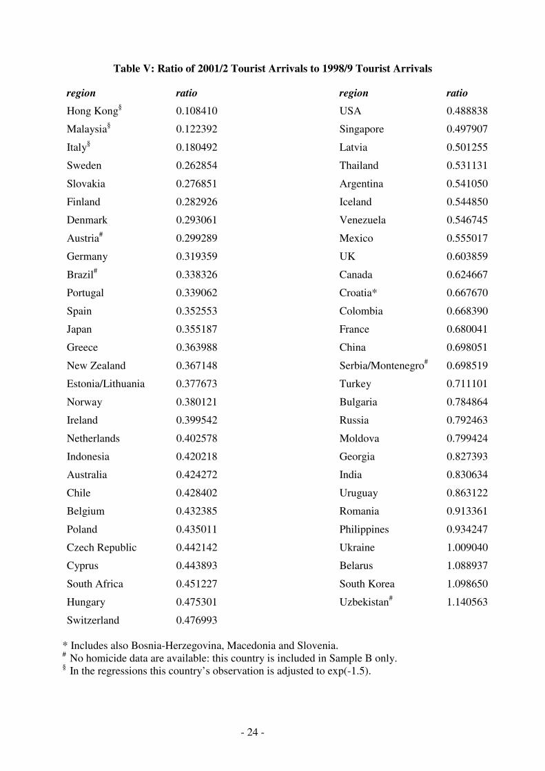
year.) The ratios (not in logs) are reported in Table V. We have excluded Arab countries from

the data set, because tourists from the Arab world might be subject to varying visa

requirements over the sample period. Otherwise, we report data from all countries listed by the

CBS for which we can measure each element of Wmk. It can be seen that there is substantial

variation in the data. For three countries – Hong Kong, Malaysia and Italy – the ratio is less

than 20%, but for another four – Ukraine, Belarus, South Korea and Uzbekistan – the ratio is

over 100%.16 That is, there were a few countries from which tourist arrivals actually increased

after the start of the Intifada. It turns out that the figures for Hong Kong, Malaysia and Italy are

outliers in the distribution of ∆ln(pmk). Inclusion of these three countries in the sample makes

the distribution of ∆ln(pmk) significantly non-normal. At the very bottom end of the distribution

there might be some non-linearity in the data generating process for ∆ln(pmk). (There are no

outliers at the other end of the distribution.) However, with only 57 observations in all we do

not have enough degrees of freedom to model non-linearities in the tail. For this reason we

adjust the figures for the three countries, raising them all to -1.5 (implying a ratio of 22% in

Table V). A discussion of alternative ways of dealing with the non-normality is available on

request: the results reported in section 4 are generally robust to the alternatives.

[Table V here]

The Jewish population figures are taken from those published at www.jewishpeople.net; PJk is

calculated by dividing these figures by the total population estimates published in the World

Bank World Development Indicators. PCYk is PPP adjusted per capita GDP in US Dollars, as

reported in the United Nations Human Development Report 2001. Ck is calculated as the ratio

of the GDP deflator in k to that in Israel, scaled by the value of the Sheqel in k-currency.

Average figures for 1998-9 and 2002-2 are calculated, and ∆ln(Ck) is the growth rate between

the two periods. ∆ln(Yk) is constructed in an analogous way, with Yk measured as real (2000)

US Dollar GDP from World Development Indicators for 1998-9 and 2001-2.

Two alternative measures of Vk are considered. The first is the log of the number of

reported homicides per 10,000 inhabitants in 2000, ln(Hk), reported in the UN World Crime

- 15 -

Survey. This is available for 53 of our 57 countries. We expect ∆ln(pmk) to be increasing in

ln(Hk). The second, available for all 57 countries, is the 2000 Rule of Law measure described in

Kaufmann et al. [2003] and here designated as ROLk. This measure aggregates national scores

awarded for the perceived level of crime in a country, the reliability of the judiciary and the

enforceability of contracts. It is therefore a very much wider and more subjective indicator of

the degree of lawlessness in society. Since higher scores are awarded to more lawful societies,

we expect ∆ln(pmk) to be decreasing in ROLk. Note that this variable is constructed as an index

ranging in value from -2.7 to +2.7, and is approximately normally distributed; it appears in the

regression in levels, not in logs.

Table VI reports the results of fitting equation (14) to the data, first of all using the

ln(Hk) measure, then using the ROLk measure. The explanatory variables account for about half

of the sample variation in ∆ln(pmk). All variables except ∆ln(Ck) and ln(Hk) are statistically

significant at the 5% level, and all significant coefficients have the anticipated sign. The

significance level for ln(Hk) is just above 10%, and it does not explain as much of the sample

variation as the alternative measure ROLk. However, with the exception of ln(PCYk), the

coefficients on other variables do not vary much between the two regression specifications.

The ln(PCYk) coefficient is sensitive to the specification because poor countries are much more

crime-ridden, so ln(Hk), ROLk and ln(PCYk) are highly correlated. When ln(Hk) and ROLk are

replaced by their corresponding orthogonal components – i.e., the residuals from regressions of

ln(Hk) and ROLk respectively on ln(PCYk) – the coefficients on ln(PCYk) in the two

specifications are almost identical. These coefficients are reported at the bottom of the table.

[Table VI here]

The table shows that if the fraction of local population that is Jewish is one percentage point

higher – for example 1% of the population instead of 2% - then the rate of decline of tourism

over the sample period is on average 40% lower. This is consistent with large but unsurprising

differences between Jews and non-Jews – on average – in terms of the deterrent effect of the

violence. More interestingly, the regression equations with orthogonalized lawlessness

indicators imply that a 10% increase in per capita income of the country of origin is associated

with a rate of decline of tourism over the sample period that is around 3.4% higher. Part – but

not all – of this effect is because a higher per capita income is associated with lower

lawlessness in a country. Some of the per capita income effect has another source; one

plausible explanation is that tourists from poor countries are more likely to be wealthier than

their neighbors, and therefore more accustomed to being targets of violence.

- 16 -

Since the Rule of Law variable is an index, the coefficient on this variable is difficult to

interpret per se. However, the sample standard deviation of ROLk is 0.97, so the estimated

coefficient shows, approximately, the effect on tourism decline of a one standard deviation

change in the index. In more law-abiding societies the decline is greater, a standard deviation

increase in ROLk being associated with an additional 17% fall. The positive coefficient on the

homicide variable ln(Hk) in the alternative regression specification is consistent with this effect,

but the standard error on the homicide coefficient is very large, so it is not quite significant at

the 10% level. Possibly this definition of lawlessness is too narrow.

Finally, despite the huge impact of the violence, tourists do seem to be sensitive to

economic conditions at the margin. Countries with the largest real income growth have showed

the smallest declines in tourism to Israel, ceteris paribus. Countries with income growth 1%

higher have shown a rate of tourism decline that is about 1.5% lower on average. However, the

coefficient on real exchange rate variable is insignificantly different from zero.

With regard to the potential differences between Europeans and Americans, the results

in this section confirm those of the previous section, answering our original question in the

negative. Table V shows that the value of ∆ln(pmk) for the USA lies in the middle range, only

one observation away from the median. Some Western European countries (mainly Nordic and

Southern Mediterranean ones, with lower crime rates and/or a smaller Jewish population) show

far larger declines in tourism to Israel than does the USA. But others (notably France and the

United Kingdom, with a lower per capita income) show substantially smaller declines. Once

we have conditioned on a set of socio-economic characteristics, the remaining variation in the

data (about half of the total variation) has no obvious socio-economic explanation and is

uncorrelated with geographical location. In the ROL regression, the estimated value of εk for

the USA is -0.18, implying a larger decline in tourism than average, conditional on the RHS

variables in equation (14). This compares with a German εk of -0.11, a French εk of 0.19 and a

British εk of 0.33; but the sample standard deviation of εk is 0.30, so none of these differences

is statistically significant. As Table VI indicates, the null that εk is normally distributed cannot

be rejected.

V. Conclusion

Analysis of time-series and cross-sectional Israeli tourist data reveals some of the factors

driving people’s attitudes towards the risk associated with travel to a conflict region. Time-

series analysis shows that since the onset of the Intifada even the relatively small variations in

conflict intensity – as measured by the number of fatalities per month – have affected tourist

- 17 -

volumes. These results reinforce previous studies of the wider macroeconomic impact of the

Intifada, for example Fielding [2003] and Eckstein and Tsiddon [2004]. This is true of both

American and European tourists, with no significant differences between the two groups. It is

consistent with a model in which, even at moderate levels of violence, a large number of

people are approximately indifferent between travelling and not travelling. As a consequence,

we can expect even a partial reduction in violent conflict in the region to boost tourism

revenue, which could be grounds for optimism regarding a gradual resolution of the conflict.

It is also worth noting that tourists are sensitive not only to deaths within Israel, but also

(to a lesser degree) deaths of both Israelis and Palestinians in the West Bank and Gaza. All

dimensions of the conflict, and not only Israeli deaths in suicide bombings, have an impact on

the Israeli economy. In our fitted model, an increase in monthly Israeli fatalities from zero to

ten deaths, such as would be caused by a large suicide bombing, would reduce American

tourist numbers by around 30% in the next month and 45% in the month following. (Thereafter

tourist numbers would swiftly recover.) The estimated effects on European tourist numbers are

of the same order of magnitude, implying to a total loss of tourist revenue in the order of

$250mn. An equivalent increase in WBG fatalities would reduce American tourist numbers by

around 15-20% in the second and third months following. Given that the monthly average

number of fatalities in WBG is 64 (as opposed to five in Israel) Palestinian deaths cost the

Israeli economy a substantial amount of money.

Analysis of cross-sectional data reveals more about the differences, and the absence of

differences, between tourists of different nationalities. Some socio-economic characteristics

(such as a high average income levels and a low crime rate) are associated with a larger decline

in tourist numbers when the violence starts. Tourists from countries at lower levels of

economic development are less sensitive to the violence. Once we have controlled for these

characteristics there is no obvious geographical pattern to the variation in tourist behaviour.

'Old Europe' demonstrates no more and no less risk aversion than the New World.

We ought to be cautious in inferring from these results about a sample of tourists

conclusions about whole populations. In many countries international tourists might not be

typical of the population in which they live. Nevertheless, the homogeneity of the time-series

regression results across European and American samples, and the extent to which the

international cross-sectional variation in tourist behaviour is associated with a few simple

socio-economic characteristics, create a strong impression that, for a given level of social and

economic welfare, people are pretty much the same everywhere.

- 18 -

Appendix 1

Here we discuss briefly our measurement of the relative cost series, which turned out never to

be statistically significant in the time-series regression equations. Data on hotel and restaurant

prices in America, Europe and Israel are available, facilitating the construction of hospitality

price real exchange rate series. However, such series are unlikely to be exogenous to total

tourist volumes, and in this context there is no obvious instrument for hotel and restaurant

prices. For this reason we measured relative costs as an aggregate consumer price real

exchange rate. For American tourists this was the log of the ratio of the Israeli consumer price

index to the Euroland consumer price index, scaled by the Shekel-Euro nominal exchange rate.

For European tourists it was the log of the ratio of the Israeli consumer price index to the US

consumer price index, scaled by the Shekel-Dollar nominal exchange rate. Nominal exchange

rate and price indices are reported by the Israeli Central Bureau of Statistics

(http://www.cbs.gov.il), the Federal Reserve Bank of St Louis

(http://research.stlouisfed.org/fred2) and the European Central Bank (http://www.ecb.int).

Substitution of a (probably endogenous) hospitality price real exchange rate for the aggregate

consumer price real exchange rate made no difference to the insignificance of relative costs in

the regression equations.

Department of Economics, University of Otago

Department of Economics, University of Leicester

- 19 -

References

G. Akerlof and Dickens, W. [1982] “The Economic Consequences of Cognitive Dissonance”,

American Economic Review 72, 307-19

A. Cukierman [2004] “Comment on: ‘Macroeconomic Consequences of Terror: Theory and the

Case of Israel’”, Journal of Monetary Economics 51, 1003-1006

K. Drakos and Kutan, A. [2003] “Regional Effects of Terrorism on Tourism in Three

Mediterranean Countries”, Journal of Conflict Resolution 47, 621-641

Z. Eckstein and Tsiddon, D. [2004] “Macroeconomic Consequences of Terror: Theory and the

Case of Israel”, Journal of Monetary Economics 51, 971-1002

W. Enders and Sandler. T. [1991] “Causality between Trans-national Terrorism and Tourism:

The Case of Spain”, Terrorism 14, 49-58

W. Enders, Sandler, T. and Parise, G. [1992] “An Econometric Analysis of the Impact of

Terrorism on Tourism”, Kyklos 45, 531-554

D. Fielding [2003] “Modelling Political Instability and Economic Performance: Israeli

Investment during the Intifada”, Economica 70, 159–186

A. Fleischer and Buccola, S. [2002] “War, Terror, and the Tourism Market in Israel”, Applied

Economics 34, 1335-1343

B. Frey, Luechinger, S. and Stutzer, A. [2004] “Calculating Tragedy: Assessing the Costs of

Terrorism”, Working Paper 205, Institute for Empirical Research in Economics, University of

Zurich

D. Kahneman, Slovic, P. and Tversky, A., eds. [1982] Judgement under Uncertainty:

Heuristics and Biases, Cambridge: Cambridge University Press

D. Kaufmann, Kraay, A. and Mastruzzi, M. [2003] “Governance Matters II: Governance

Indicators for 1996-2002”, World Bank Policy Research Department Working Paper

G. Maddala [1983] Limited Dependent and Qualitative Variables in Econometrics, Cambridge,

England: Cambridge University Press

H. Pesaran, Shin, Y. and Smith, R. [2001] “Bounds Testing Approaches to the Analysis of

Level Relationships” Journal of Applied Econometrics, 16, 289-326

B. Sloboda [2003] “Assessing the Effects of Terrorism on Tourism by Use of Time Series

Methods”, Tourism Economics 9, 179-190

C. Sunstein [2003] “Terrorism and Probability Neglect” Journal of Risk and Uncertainty 26,

121-136

W. Viscusi and Zeckhauser, R. [2003] “Sacrificing Civil Liberties to Reduce Terrorism Risks”,

Journal of Risk and Uncertainty 26, 99-120

- 20 -

Table I: Sample Statistics 3½ Years Before and After the Al-Aqsa Intifada

1997m3-2000m8 2000m9-2004m2

mean s.d. mean s.d. difference

ln(pmt/pnt) (America) -9.4967 0.2758 -10.4073 0.4416 -0.9106

ln(pmt/pnt) (Europe) -9.0252 0.3087 -10.0658 0.3993 -1.0406

ln(fmt) 0.6885 0.7413 4.1661 0.6565 3.4776

ln(zmt) 0.2142 0.5525 1.5756 1.2755 1.3614

- 21 -

Table II: American Tourist Time-Series Regression Results

Standard errors are calculated using White’s heteroskedasticity correction.

A. Unrestricted equation for ∆ln(pmt / pnt)

variable coefficient standard error t ratio partial R2

∆ln(pmt-1/pnt-1) 0.02831 0.08276 0.34207 0.0050

∆ln(zmt) -0.12125 0.04538 -2.67188 0.2349

∆ln(zmt-1) 0.00951 0.05351 0.17772 0.0021

∆ln(fmt) -0.01666 0.02165 -0.76952 0.0179

∆ln(fmt-1) 0.06924 0.02183 3.17178 0.2007

ln(pmt-1/pnt-1) -1.04140 0.10229 -10.18090 0.7547

ln(zmt-1) -0.32112 0.04594 -6.98999 0.5640

ln(fmt-1) -0.17344 0.03714 -4.66990 0.5006

DGWt -1.03030 0.12059 -8.54383 0.6069

R2 = 0.94728; σ = 0.13469

LM residual autocorrelation test: F(1,20) = 0.62967 [0.4368]

LM ARCH test: F(1,19) = 0.00001 [0.9931]

Residual normality test: χ2(2) = 2.2101 [0.3312]

F-statistic for joint significance of levels variables: F(3,21) = 22.768

B. Restricted equation for ∆ln(pmt / pnt)

variable coefficient standard error t ratio partial R2

∆ln(zmt) -0.12484 0.04101 -3.04414 0.2581

∆ln(fmt-1) 0.07492 0.01693 4.42528 0.2685

ln(pmt-1/pnt-1) -1.00750 0.07259 -13.87930 0.8475

ln(zmt-1) -0.31863 0.03648 -8.73438 0.6889

ln(fmt-1) -0.16160 0.02390 -6.76151 0.5190

DGWt -1.01760 0.10459 -9.72942 0.6011

R2 = 0.94601; σ = 0.12751

LM residual autocorrelation test: F(1,23) = 0.52302 [0.4768]

LM ARCH test: F(1,22) = 0.19195 [0.6656]

Normality test: χ2(2) = 1.0137 [0.6024]

pmt / pnt ratio of US tourists in Israel to US tourists in Europe

fmt 1 + total Israeli and Palestinian fatalities in West Bank & Gaza

zmt 1 + total fatalities in Israel

DGWt dummy variable = 1 in 2003m3, = 0 else

- 22 -

Table III: European Tourist Time-Series Regression Results

Standard errors are calculated using White’s heteroskedasticity correction.

A. Unrestricted equation for ∆ln(pmt / pnt)

variable coefficient standard error t ratio partial R2

∆ln(pmt-1/pnt-1) -0.10059 0.08268 -1.21662 0.0475

∆ln(zmt) -0.04037 0.05112 -0.78971 0.0248

∆ln(zmt-1) -0.00547 0.06146 -0.08900 0.0004

∆ln(fmt) 0.00093 0.02454 0.03790 0.0000

∆ln(fmt-1) 0.02278 0.02520 0.90397 0.0199

ln(pmt-1/pnt-1) -0.68139 0.09645 -7.06470 0.5759

ln(zmt-1) -0.29780 0.06944 -4.28859 0.4544

ln(fmt-1) -0.04624 0.03411 -1.35561 0.0571

DGWt -0.84095 0.07174 -11.72220 0.4305

R2 = 0.90854; σ = 0.15492

LM residual autocorrelation test: F(1,20) = 0.64525 [0.4313]

LM ARCH test: F(1,19) = 1.05240 [0.3178]

Normality test: χ2(2) = 0.08624 [0.9578]

F-statistic for joint significance of levels variables: F(3,21) = 10.395

B. Restricted equation for ∆ln(pmt / pnt)

variable coefficient standard error t ratio partial R2

ln(pmt-1/pnt-1) -0.69345 0.05716 -12.1317 0.7528

ln(zmt-1) -0.27551 0.04857 -5.67243 0.6834

ln(fmt-1) -0.03583 0.02657 -1.34851 0.0626

DGWt -0.85763 0.06402 -13.3963 0.4350

R2 = 0.89462; σ = 0.14945

LM residual autocorrelation test: F(1,25) = 0.00055 [0.9815]

LM ARCH test: F(1,24) = 0.01799 [0.8944]

Normality test: χ2(2) = 0.23485 [0.8892]

pmt / pnt ratio of Euro tourists in Israel to Euro tourists in the US

fmt 1 + total Israeli and Palestinian fatalities in West Bank & Gaza

zmt 1 + total fatalities in Israel

DGWt dummy variable = 1 in 2003m3, = 0 else

- 23 -

Table IV: Long-Run Levels Elasticities in the Unrestricted Models

ln(zm) ln(fm) DGW

US equation -0.30835 -0.16654 -0.98934

Standard error 0.04838 0.03255 0.20792

European equation -0.43705 -0.06787 -1.23420

Standard error 0.09012 0.05803 0.36834

- 24 -

Table V: Ratio of 2001/2 Tourist Arrivals to 1998/9 Tourist Arrivals

region ratio region ratio

Hong Kong§ 0.108410 USA 0.488838

Malaysia§ 0.122392 Singapore 0.497907

Italy§ 0.180492 Latvia 0.501255

Sweden 0.262854 Thailand 0.531131

Slovakia 0.276851 Argentina 0.541050

Finland 0.282926 Iceland 0.544850

Denmark 0.293061 Venezuela 0.546745

Austria# 0.299289 Mexico 0.555017

Germany 0.319359 UK 0.603859

Brazil# 0.338326 Canada 0.624667

Portugal 0.339062 Croatia* 0.667670

Spain 0.352553 Colombia 0.668390

Japan 0.355187 France 0.680041

Greece 0.363988 China 0.698051

New Zealand 0.367148 Serbia/Montenegro# 0.698519

Estonia/Lithuania 0.377673 Turkey 0.711101

Norway 0.380121 Bulgaria 0.784864

Ireland 0.399542 Russia 0.792463

Netherlands 0.402578 Moldova 0.799424

Indonesia 0.420218 Georgia 0.827393

Australia 0.424272 India 0.830634

Chile 0.428402 Uruguay 0.863122

Belgium 0.432385 Romania 0.913361

Poland 0.435011 Philippines 0.934247

Czech Republic 0.442142 Ukraine 1.009040

Cyprus 0.443893 Belarus 1.088937

South Africa 0.451227 South Korea 1.098650

Hungary 0.475301 Uzbekistan# 1.140563

Switzerland 0.476993 * Includes also Bosnia-Herzegovina, Macedonia and Slovenia. # No homicide data are available: this country is included in Sample B only. § In the regressions this country’s observation is adjusted to exp(-1.5).

- 25 -

Table VI: Cross Section Regression Results

The dependent variable is ∆ln(pmk).

Standard errors are calculated using White’s heteroskedasticity correction.

Sample A (53 observations)

variable coefficient standard

error t ratio partial R2

intercept 1.5214 0.6717 2.2651 0.0711

ln(1+PJk).100 0.4305 0.1007 4.2764 0.1514

ln(PCYk) -0.2729 0.0656 -4.1617 0.1952

∆ln(Ck) -0.4289 0.3631 -1.1811 0.0199

∆ln(Yk) 1.5398 0.7296 2.1106 0.0749

ln(Hk) 0.0766 0.0462 1.6576 0.0452

R2 0.4597

σ 0.3228

χ2(2) residual normality test 2.3913

RESET Test: F(3,44) 0.6622

Sample B (57 observations)

variable coefficient standard

error t ratio partial R2

intercept 0.8885 0.6646 1.3369 0.0267

ln(1+PJk).100 0.4526 0.1020 4.4363 0.1729

ln(PCYk) -0.1826 0.0739 -2.4709 0.0846

∆ln(Ck) -0.2302 0.2395 -0.9611 0.0123

∆ln(Yk) 1.3228 0.5687 2.3260 0.0655

ROLk -0.1726 0.0515 -3.3544 0.1118

R2 0.5258

σ 0.3091

χ2(2) residual normality test 3.0845

RESET Test: F(3,48) 0.7440

ln(PCYk) regression coefficients when ln(Hk) and ROLk are orthogonalized

coefficient standard

error t ratio partial R2

Sample A -0.3452 0.045497 -7.58687 0.4494

Sample B -0.3405 0.051402 -6.62464 0.3896

- 26 -

1/z2 1/z11/z

g

Figure 1a

1/z 1/z2 1

1/z

g

Figure 1b

- 27 -

2001 2002 2003 2004

-11

-10.5

-10

-9.5

-9

Figure 2: Tourism series ln(pmt/pnt) 2000m9-2004m2:

Americans (■) and Europeans (○)

2001 2002 2003 2004

1

2

3

4

5

6

Figure 3: Fatality series 2000m9-2004m2: ln(zmt)(○) and ln(fmt)(■)

- 28 -

2003 2004

-.2

-.1

0

.1

.2

Figure 4: One-step American sample forecast errors with 2 s.e. bars (2003m2–2004m2)

2003 2004

-.3

-.2

-.1

0

.1

.2

.3

Figure 5: One-step European sample forecast errors with 2 s.e. bars (2003m2–2004m2)

- 29 -

2003 2004

-.5

-.4

-.3

-.2

2003 2004

-.2

-.1

0

Figure 6: Recursive estimates of the ln(zmt-1)(■) and ln(fmt-1)(○) coefficients, American sample

2003 2004

-.5

-.4

-.3

-.2

-.1

2003 2004

-.2

-.1

0

.1

.2

Figure 7: Recursive estimates of the ln(zmt-1)(■) and ln(fmt-1)(○) coefficients, European sample

- 30 -

0 1 2 3 4 5 6

-.15

-.1

-.05

0

0 1 2 3 4 5 6

-.075

-.05

-.025

0

Figure 8: Response of ln(pmt/pnt) to a unit increase in ln(zmt)(■) and ln(fmt)(○), American sample

0 1 2 3 4 5 6

-.2

-.1

0

0 1 2 3 4 5 6

-.02

-.01

0

Figure 9: Response of ln(pmt/pnt) to a unit increase in ln(zmt)(■) and ln(fmt)(○), European sample

- 31 -

Notes

§. We are grateful for the support of ESRC Grant RES-000-22-0312, which funded the project of which

this paper is a part. Thanks also to Paul Frijters, Paul Hansen and Frank Stähler, and to seminar participants at the Universities of Leicester and Otago for comments on previous drafts of this paper. All remaining errors and omissions are our own.

1. In any case, there is substantial evidence from studies of individual respondents that people’s response to the risk of injury in a violent political conflict does not square with Expected Utility Theory, and that they place 'excessive' weight on highly improbable states of the world with very low utility. Sunstein [2003] and Viscusi and Zeckhauser [2003] find that people assessing conflict risk are prone to deviations from EUT common in other risk perception contexts; so their behaviour might be better explained by, for example, Prospect Theory.

2. The quotation is from a speech by M. Daniels, Office of Management and Budget, The Executive Office of the President, May 16 2003 (http://www.whitehouse.gov/omb/speeches/daniels051603.html).

3. The number of tourist arrivals is a little higher than the number checking into hotels, because some tourists do not stay in hotels; for example, some stay with friends or family. However, data from the two sources – hotels and immigration – are broadly consistent. Some monthly tourist arrival statistics reported by immigration are published in the CBS Monthly Bulletin of Statistics, but only for selected months.

4. The regression specification we end up with is similar in spirit to that of Fleischer and Buccola [2002], who analyze total foreign demand for Israeli hotel accommodation up to 1999, but differs from theirs in points of detail. They do not formulate an explicit discrete choice model, and do not disaggregate foreign hotel guests by nationality. They condition demand for hotel beds on a single lagged “terror index”, and on foreign income and tourist expenditure outside Israel (rather than tourist volumes outside Israel). We contend that it is more appropriate to use tourist volumes outside Israel as a scale variable when modelling tourist volumes inside Israel. They also condition on Israeli hotel prices, using Israeli hotel wages as an instrument. We are not sure that wages are really exogenous to the demand for hotel beds and anyway, as documented below, we find prices to be statistically insignificant in the post-2000 period.

5. Of course many tourists may lay the blame for the conflict on the Palestinian authorities, or on militant Palestinian groups; this would affect the number of tourists visiting WBG, if there were any to start with.

6. We take this approach with f as well as with z: there is no reason why the intensity of political disapproval should be based on a backward-looking measure of conflict intensity.

7. There is likely also to be some seasonality in w. Such seasonality should be taken as implicit in equations (8-10), and is accounted for in the regressions in section 3.2.

8. Not everywhere in Europe is safe, but most of the places we see American tourists are pretty quiet. 9. It does affect our estimated short-run dynamics. Further results are available on request. 10. The validity of this approach relies on the existence of a single levels relationship. Appendix 2 shows

that there is no levels relationship between ln(z) and ln(f) as we measure them. 11. These are OLS estimates; FIML estimates allowing for the non-zero equation residual correlations

are very similar. 12. Using data for the period 1988(2)-2004(5), the DF t-statistic for the seasonally adjusted ln(RTF)

series is -12.19. 13. Nevertheless, such an asymmetry is consistent with the economic psychology of Kahneman et al.

[1982], in which larger subjective probabilities are assigned to types of events, such as suicide bombings, that are more memorable.

14. Note that this assumption is consistent with some cross-sectional variation in the level of desirability of different locations; such variation is differenced out in our model.

15. No real income variable is included in the time-series model, which scales tourist volumes in Israel by tourist volumes in a reference location. This exclusion would be invalid only if the income elasticity of demand for international vacations varied with destination. When an income term is added to the time-series regression equations it is statistically insignificant: there is no reason to suppose that there is any such variation in income elasticities.

16. The presence of South East Asian countries in both of these lists suggest that pure geographical factors are unlikely to be important determinants of ∆ln(p). When regional dummies are added to the regression equations reported in section 4, they are individually and jointly insignificant, including the former Soviet Union dummy. Nor is the rate of decline in numbers correlated with the original size of the tourist population: the t-ratio for the correlation of ∆ln(p) and the log of tourist numbers in 1998-99 is -1.514.