DEPARTMENT OF ECONOMICS

Working Paper

UNIVERSITY OF MASSACHUSETTS

AMHERST

Institutional shocks and economic outcomes: Allende’s election,

Pinochet’s coup and the Santiago stock market

Daniele Girardi Samuel Bowles

Working Paper 2017-19

Institutional shocks and economic outcomes: Allende’s

election, Pinochet’s coup and the Santiago stock market

Daniele Girardi

⇤Samuel Bowles

†

Abstract

To study the e↵ect of political and institutional changes on the economy, we

look at share prices in the Santiago exchange during the tumultuous political events

that characterized Chile in the early 1970s. We use a transparent empirical strat-

egy, deploying previously unused daily data and exploiting two largely unexpected

shocks which involved substantial variation in policies and institutions, providing

a rare natural experiment. Allende’s election and subsequent socialist experiment

decreased share values, while the military coup and dictatorship that replaced him

boosted them, in both cases by magnitudes unprecedented in the literature.

JEL Codes: P00 (Economics Systems), P16 (Political Economy), D02 (Institutions:

Design, Formation, Operations, and Impact), E02 (Institutions and the Macroeconomy),

N2 (Economic History - Financial Markets and Institutions).

Keywords: institutional shocks, natural experiment, share prices, Chile, socialism,

military coup, elections.

⇤University of Massachusetts – Amherst, email: dgirardi@umass.edu†Santa Fe Institute, email: samuel.bowles@gmail.com

We are grateful to Manuel Agosin, Arin Dube, Manuel Garcia, Oscar Landerretche, Juan AntonioMontecino, Peter Skott, Barbara Stallings and Suresh Naidu for comments and suggestions on previousdrafts of this paper. All remaining errors are of course our own.

1

12 September, 1970:

Kissinger: “The big problem today is Chile”

Nixon: “Their stock market went to hell”

1 Introduction

The election of Salvador Allende’s socialist government in Chile in 1970 and its subse-

quent reversal by a military coup in 1973 provide a curiously unexploited opportunity to

study the e↵ect of institutional shocks on economic outcomes.1 Unidad Popular (UP),

the left-wing political coalition that supported Allende, promised, and after elected took

steps to implement profound changes to economic institutions and the structure of prop-

erty rights, towards the final goal of replacing capitalism with some form of socialism.

The military coup ended Allende’s socialist experiment and promised a return to pro-

business policies, but now under authoritarian rule.2

From a research standpoint, the importance of these events lies not only in the large

institutional and policy variation involved, but also in the fact that the outcome of the

1970 election was a surprise. Prior to the election, for example, the leading daily El

Mercurio had published a number of polls showing Jorge Alessandri (a rightwing inde-

pendent who had been president from 1958 to 1964) leading Allende by a considerable

margin (Table 1). We will use data from vote expectation surveys to show that the

perceived probability of a socialist victory was indeed rather low, particularly among

potential shareholders (Tables 4 and 5).3 Moreover, while an attempt to remove Allende

from power was expected by many, an attempted military coup had already failed earlier

in the year, so the success of the coup in September 1973 could not have been entirely

anticipated.

Natural experiments allowing convincing identification of the e↵ect of sharp changes

in economic institutions on the valuation of assets seldom arise. As a result of Hotelling-

1The epigraph is from a 12:32pm telephone conversation in Washington. Source: Library of Congress,Manuscript Division, Kissinger Papers, Box 364

2Major sources on the history of the Allende government and of the military coup are Stallings (1978);Sigmund (1977); Nef (1983); Larrain and Meller (1991)

3Besides the quantitative evidence that we will provide here, the fact that the Allende victory waslargely unexpected is reported also in Sigmund (1977, pp. 106-110); Marash (1988); Navia (2004); Hersh(1983, p. 273); NSC (1970).

2

Downs pressures for platform convergence (Downs, 1957), in closely contested elections

with uncertain outcomes party programs are rarely radically di↵erent when it comes

to fundamental economic institutions. Non-electoral institutional shocks, such as those

arising from a revolutionary transfer of power, are rarely unanticipated and are typically

associated with other relevant changes that confound the pure ’institution shock e↵ect’,

making identification virtually impossible.

To assess the stock-market reaction to these two shocks we employ daily data on

the General Index of Stock Prices (IGPA) calculated by the Santiago exchange, a

capitalization-weighted index that includes most listed companies. Historical daily data

on the IGPA index is proprietary, and we purchased it from the Santiago exchange. We

complement this information with newly digitized data on individual stocks.4

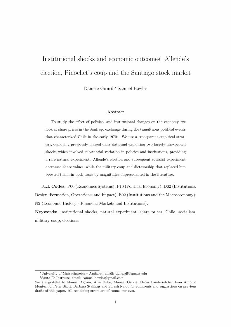
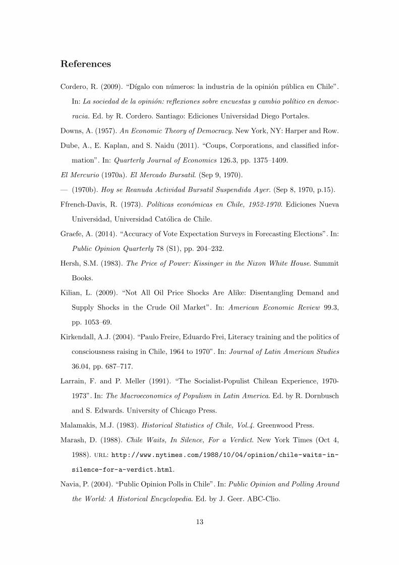
Figure 1 displays the IGPA in a long window around our period of interest. Hav-

ing risen under Alessandri, stock market valuations had declined during the presidency

of Eduardo Frei Montalva (1964-1970), a Christian Democratic leader who enacted re-

distributive policies, most notably in the areas of education, land reform and taxation

(Ffrench-Davis, 1973; Kirkendall, 2004; Thome, 1971). They decreased further during

Allende’s socialist presidency, before experiencing a strong revival after the military

coup.

2 The Unidad Popular electoral victory

Allende’s margin of victory over the runner-up Alessandri in the 1970 election was just

1.34%.5 Respecting a longstanding political tradition, Allende would later be confirmed

as president.

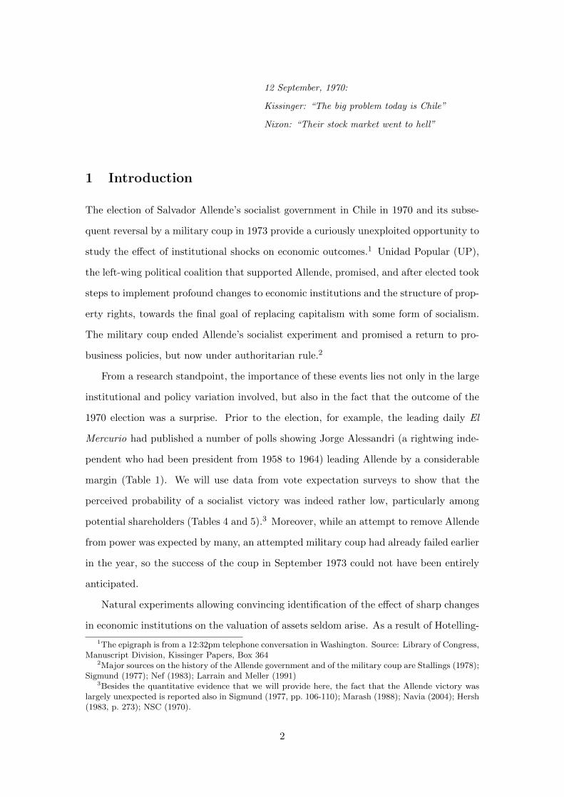
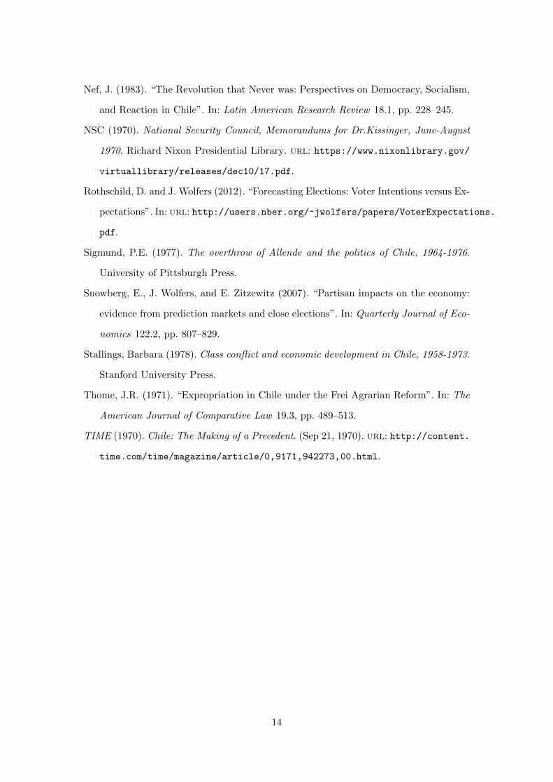
In the first trading day after the election,6 the IGPA fell by 22%. This constitutes

4We hand-collected data on the daily prices of individual stocks listed in the Santiago exchange fromcopies of the Chilean newspaper El Mercurio, which we accessed in microfilm format at Yale Universitylibrary.

5Allende 36.61%; Alessandri 35.27%; Tomic (Christian Democratic) 28.11%.6This was Tuesday September 8: the market was closed the Monday after the election. Although the

management of the stock exchange declared that activity had been interrupted because of “technicalreasons” (El Mercurio, 1970b), contemporary observers countered that the stock market had actuallybeen closed in an attempt to mitigate financial panic due to the election outcome. For example, the USmagazine TIME wrote that “fearful of a stampede of scared investors, the Santiago stock market closedfor a day for the first time since 1938.”. (TIME, 1970)

3

the largest daily decrease in share prices ever recorded in Santiago in the period for

which we have data (1961-2016). Compared with the empirical distribution of daily

fluctuations in the IGPA until that day, this daily change is 25.8 standard deviations

below the sample mean (16.1 standard deviations if considering the whole 1961-2016

period), and in absolute value is 2.5 times larger than the previous maximum deviation.

Figure 2 displays trading days before and after the election on the horizontal axis (with

the first trading day after the event equal to zero) and the IGPA index on the vertical

axis. For ease of interpretation, a vertical red dashed line corresponds to the last trading

day before the election.

Stock prices kept falling for around 15 trading days after the event, and stabilized

at a much lower level around the end of the month. Between September 3 1970 (the last

trading day before the election) and September 30, the IGPA fell by 48.6 percentage

points.

The behavior of individual stocks suggests that the continuing substantial decline

in share values in the days immediately after the ‘Allende shock’ was partly due to the

fact that many stocks were not traded at all in the immediate aftermath of the election.

According to the daily commentary of stock-market activity published on El Mercurio,

the market was partly frozen in the first trading day after the election, with would-be

sellers struggling to find buyers (El Mercurio, 1970a).

Indeed, out of 167 listed firms that we observe both immediately before and imme-

diately after the election, only 32 were e↵ectively exchanged in the first trading day

after the election. Those shares decreased on average by 40.8% that day, and then by a

further 17.8% in the rest of the month. For those stocks, therefore, we do observe sub-

stantial delayed adjustment, but the bulk of the decrease happened immediately. The

part of the adjustment which was not immediate may be explained by the acquisition

of new information in the aftermath of the election – for example the growing certainty

that Allende would be confirmed as President by the National Congress – and/or by the

fact that it took some time for investors to fully ‘digest’ the consequences of an Allende

presidency.

The 96 stocks that were not exchanged in the first trading day after the election,

4

but were then exchanged in the rest of the month, fell on average by 37.1 percentage

points between election day and September 30.

Importantly, as shown in Table 2, the fall in share prices was broad, with little dif-

ferences across industries. Among the seven sectors in which firms were classified by

contemporary sources, the standard deviation of the percentage change in valuations

is just 10.3% of the average change. This suggests that shareholders’ concerns about

property rights and profitability in publicly-held firms were pervasive across the whole

economy, not just in sectors explicitly targeted for nationalization, such as banking,

insurance and mining.

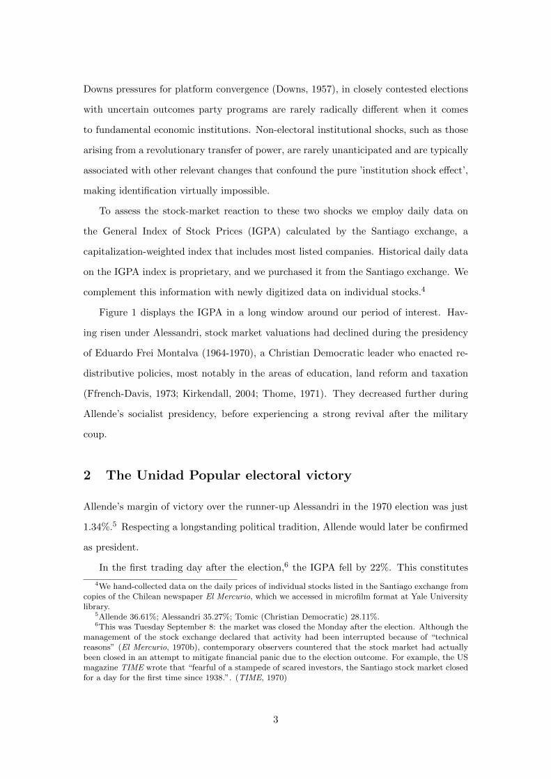
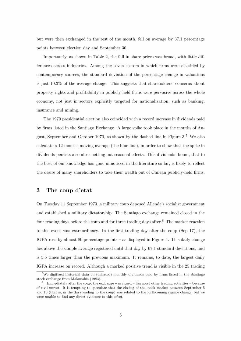
The 1970 presidential election also coincided with a record increase in dividends paid

by firms listed in the Santiago Exchange. A large spike took place in the months of Au-

gust, September and October 1970, as shown by the dashed line in Figure 3.7 We also

calculate a 12-months moving average (the blue line), in order to show that the spike in

dividends persists also after netting out seasonal e↵ects. This dividends’ boom, that to

the best of our knowledge has gone unnoticed in the literature so far, is likely to reflect

the desire of many shareholders to take their wealth out of Chilean publicly-held firms.

3 The coup d’etat

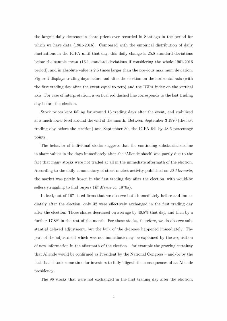
On Tuesday 11 September 1973, a military coup deposed Allende’s socialist government

and established a military dictatorship. The Santiago exchange remained closed in the

four trading days before the coup and for three trading days after.8 The market reaction

to this event was extraordinary. In the first trading day after the coup (Sep 17), the

IGPA rose by almost 80 percentage points – as displayed in Figure 4. This daily change

lies above the sample average registered until that day by 67.1 standard deviations, and

is 5.5 times larger than the previous maximum. It remains, to date, the largest daily

IGPA increase on record. Although a marked positive trend is visible in the 25 trading

7We digitized historical data on (deflated) monthly dividends paid by firms listed in the Santiagostock exchange from Malamakis (1983).

8 Immediately after the coup, the exchange was closed – like most other trading activities – becauseof civil unrest. It is tempting to speculate that the closing of the stock market between September 5and 10 (that is, in the days leading to the coup) was related to the forthcoming regime change, but wewere unable to find any direct evidence to this e↵ect.

5

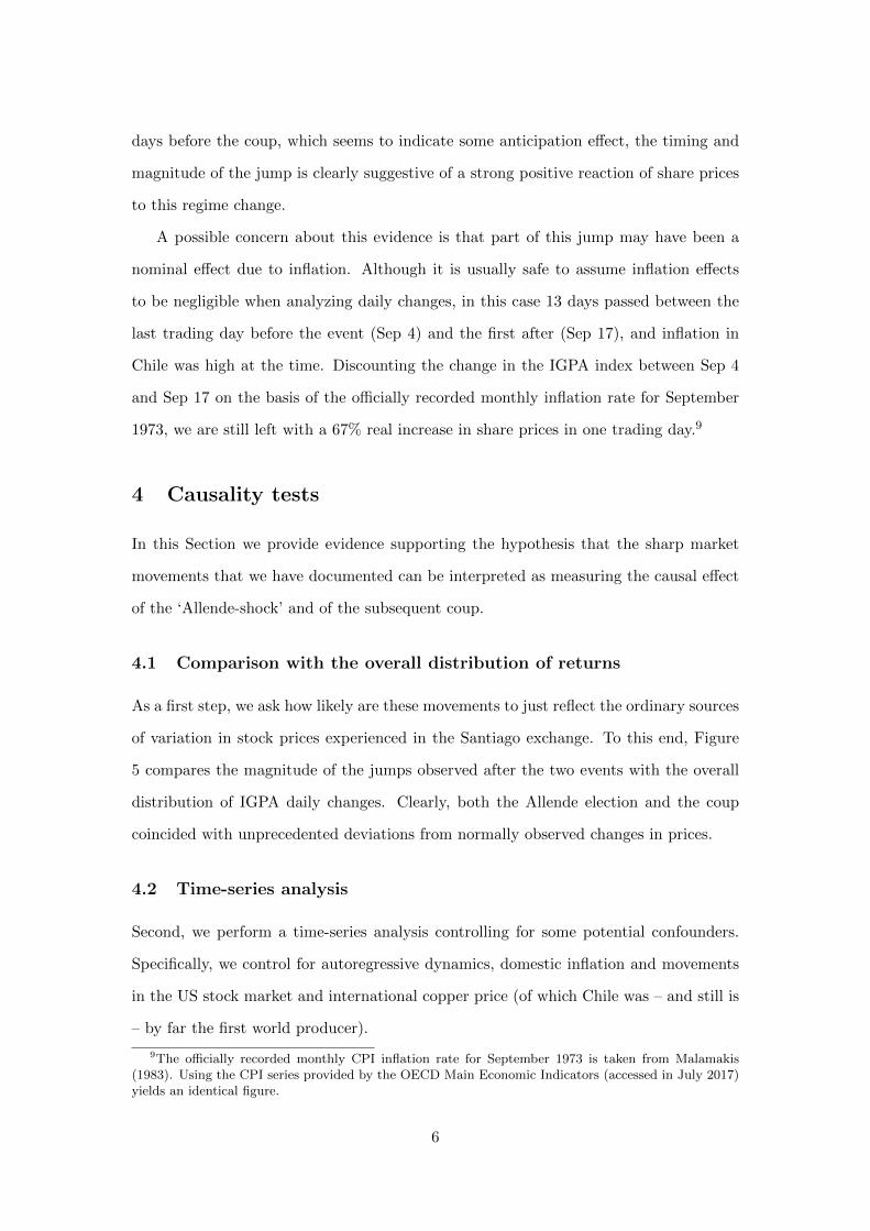
days before the coup, which seems to indicate some anticipation e↵ect, the timing and

magnitude of the jump is clearly suggestive of a strong positive reaction of share prices

to this regime change.

A possible concern about this evidence is that part of this jump may have been a

nominal e↵ect due to inflation. Although it is usually safe to assume inflation e↵ects

to be negligible when analyzing daily changes, in this case 13 days passed between the

last trading day before the event (Sep 4) and the first after (Sep 17), and inflation in

Chile was high at the time. Discounting the change in the IGPA index between Sep 4

and Sep 17 on the basis of the o�cially recorded monthly inflation rate for September

1973, we are still left with a 67% real increase in share prices in one trading day.9

4 Causality tests

In this Section we provide evidence supporting the hypothesis that the sharp market

movements that we have documented can be interpreted as measuring the causal e↵ect

of the ‘Allende-shock’ and of the subsequent coup.

4.1 Comparison with the overall distribution of returns

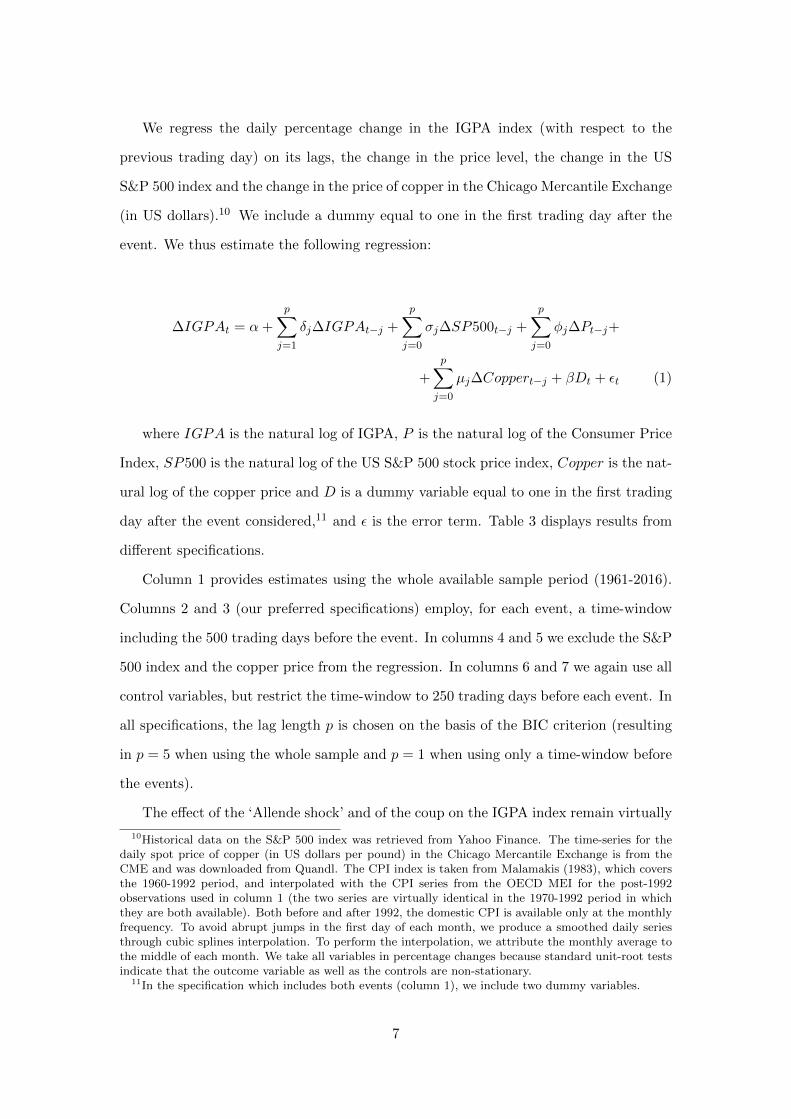
As a first step, we ask how likely are these movements to just reflect the ordinary sources

of variation in stock prices experienced in the Santiago exchange. To this end, Figure

5 compares the magnitude of the jumps observed after the two events with the overall

distribution of IGPA daily changes. Clearly, both the Allende election and the coup

coincided with unprecedented deviations from normally observed changes in prices.

4.2 Time-series analysis

Second, we perform a time-series analysis controlling for some potential confounders.

Specifically, we control for autoregressive dynamics, domestic inflation and movements

in the US stock market and international copper price (of which Chile was – and still is

– by far the first world producer).

9The o�cially recorded monthly CPI inflation rate for September 1973 is taken from Malamakis(1983). Using the CPI series provided by the OECD Main Economic Indicators (accessed in July 2017)yields an identical figure.

6

We regress the daily percentage change in the IGPA index (with respect to the

previous trading day) on its lags, the change in the price level, the change in the US

S&P 500 index and the change in the price of copper in the Chicago Mercantile Exchange

(in US dollars).10 We include a dummy equal to one in the first trading day after the

event. We thus estimate the following regression:

�IGPAt = ↵+pX

j=1

�j�IGPAt�j +pX

j=0

�j�SP500t�j +pX

j=0

�j�Pt�j+

+pX

j=0

µj�Coppert�j + �Dt + ✏t (1)

where IGPA is the natural log of IGPA, P is the natural log of the Consumer Price

Index, SP500 is the natural log of the US S&P 500 stock price index, Copper is the nat-

ural log of the copper price and D is a dummy variable equal to one in the first trading

day after the event considered,11 and ✏ is the error term. Table 3 displays results from

di↵erent specifications.

Column 1 provides estimates using the whole available sample period (1961-2016).

Columns 2 and 3 (our preferred specifications) employ, for each event, a time-window

including the 500 trading days before the event. In columns 4 and 5 we exclude the S&P

500 index and the copper price from the regression. In columns 6 and 7 we again use all

control variables, but restrict the time-window to 250 trading days before each event. In

all specifications, the lag length p is chosen on the basis of the BIC criterion (resulting

in p = 5 when using the whole sample and p = 1 when using only a time-window before

the events).

The e↵ect of the ‘Allende shock’ and of the coup on the IGPA index remain virtually

10Historical data on the S&P 500 index was retrieved from Yahoo Finance. The time-series for thedaily spot price of copper (in US dollars per pound) in the Chicago Mercantile Exchange is from theCME and was downloaded from Quandl. The CPI index is taken from Malamakis (1983), which coversthe 1960-1992 period, and interpolated with the CPI series from the OECD MEI for the post-1992observations used in column 1 (the two series are virtually identical in the 1970-1992 period in whichthey are both available). Both before and after 1992, the domestic CPI is available only at the monthlyfrequency. To avoid abrupt jumps in the first day of each month, we produce a smoothed daily seriesthrough cubic splines interpolation. To perform the interpolation, we attribute the monthly average tothe middle of each month. We take all variables in percentage changes because standard unit-root testsindicate that the outcome variable as well as the controls are non-stationary.

11In the specification which includes both events (column 1), we include two dummy variables.

7

unchanged across all regressions, and very close to the unconditional changes observed

in the first trading day after the events (-21.88% and +79.20%, respectively). We con-

clude that US macroeconomic conditions, the international copper market and domestic

inflation did not contribute in any meaningful way to the jumps in stock market values

observed after the institutional shocks examined.12

4.3 Panel two-way fixed e↵ects regression

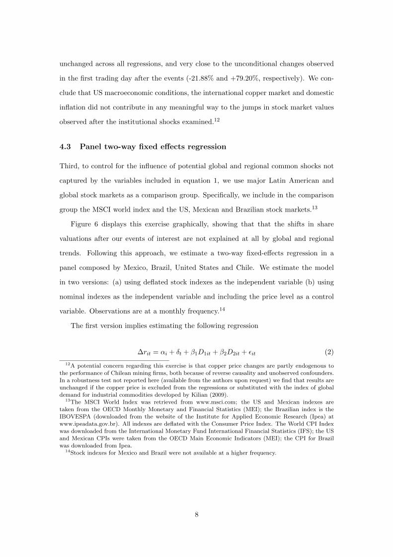
Third, to control for the influence of potential global and regional common shocks not

captured by the variables included in equation 1, we use major Latin American and

global stock markets as a comparison group. Specifically, we include in the comparison

group the MSCI world index and the US, Mexican and Brazilian stock markets.13

Figure 6 displays this exercise graphically, showing that that the shifts in share

valuations after our events of interest are not explained at all by global and regional

trends. Following this approach, we estimate a two-way fixed-e↵ects regression in a

panel composed by Mexico, Brazil, United States and Chile. We estimate the model

in two versions: (a) using deflated stock indexes as the independent variable (b) using

nominal indexes as the independent variable and including the price level as a control

variable. Observations are at a monthly frequency.14

The first version implies estimating the following regression

�rit = ↵i + �t + �

1

D

1it + �

2

D

2it + ✏it (2)

12A potential concern regarding this exercise is that copper price changes are partly endogenous tothe performance of Chilean mining firms, both because of reverse causality and unobserved confounders.In a robustness test not reported here (available from the authors upon request) we find that results areunchanged if the copper price is excluded from the regressions or substituted with the index of globaldemand for industrial commodities developed by Kilian (2009).

13The MSCI World Index was retrieved from www.msci.com; the US and Mexican indexes aretaken from the OECD Monthly Monetary and Financial Statistics (MEI); the Brazilian index is theIBOVESPA (downloaded from the website of the Institute for Applied Economic Research (Ipea) atwww.ipeadata.gov.br). All indexes are deflated with the Consumer Price Index. The World CPI Indexwas downloaded from the International Monetary Fund International Financial Statistics (IFS); the USand Mexican CPIs were taken from the OECD Main Economic Indicators (MEI); the CPI for Brazilwas downloaded from Ipea.

14Stock indexes for Mexico and Brazil were not available at a higher frequency.

8

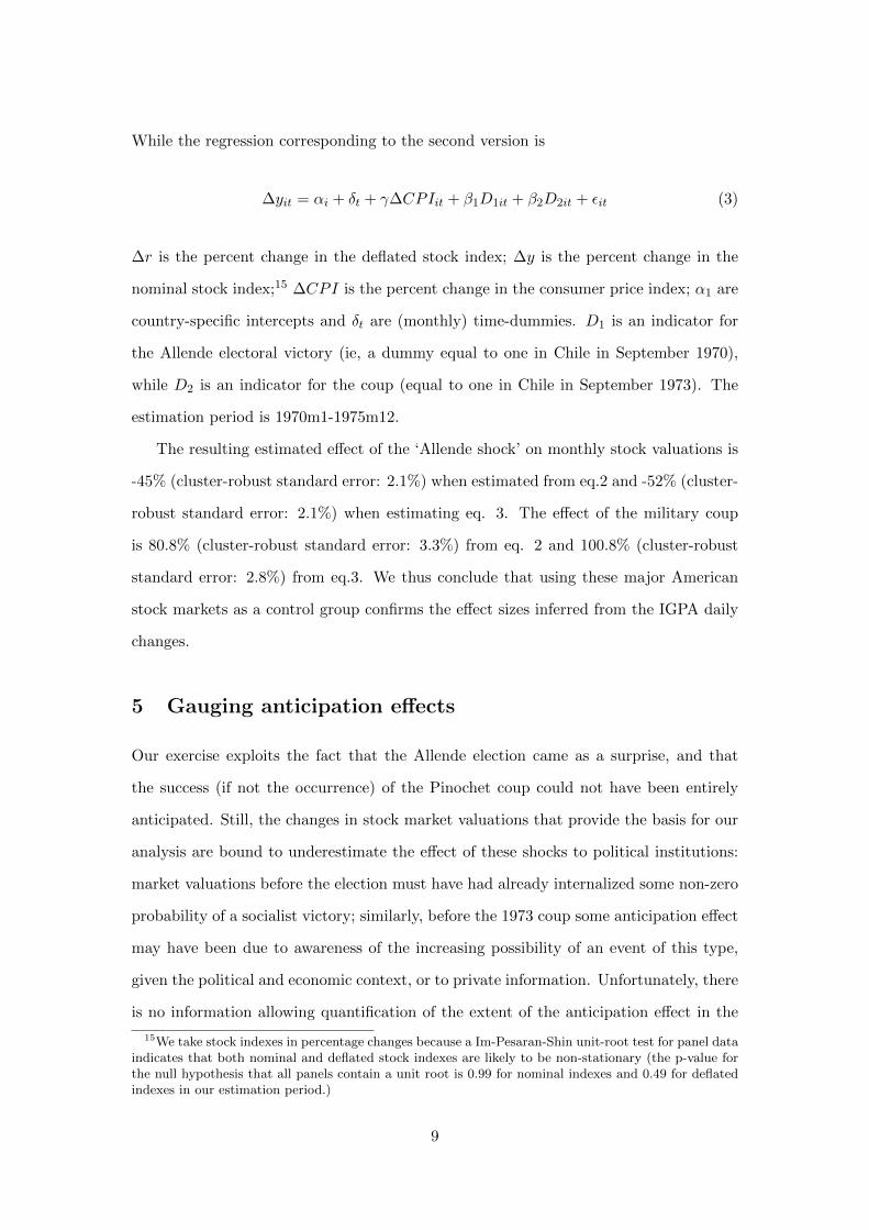
While the regression corresponding to the second version is

�yit = ↵i + �t + ��CPIit + �

1

D

1it + �

2

D

2it + ✏it (3)

�r is the percent change in the deflated stock index; �y is the percent change in the

nominal stock index;15 �CPI is the percent change in the consumer price index; ↵1

are

country-specific intercepts and �t are (monthly) time-dummies. D

1

is an indicator for

the Allende electoral victory (ie, a dummy equal to one in Chile in September 1970),

while D

2

is an indicator for the coup (equal to one in Chile in September 1973). The

estimation period is 1970m1-1975m12.

The resulting estimated e↵ect of the ‘Allende shock’ on monthly stock valuations is

-45% (cluster-robust standard error: 2.1%) when estimated from eq.2 and -52% (cluster-

robust standard error: 2.1%) when estimating eq. 3. The e↵ect of the military coup

is 80.8% (cluster-robust standard error: 3.3%) from eq. 2 and 100.8% (cluster-robust

standard error: 2.8%) from eq.3. We thus conclude that using these major American

stock markets as a control group confirms the e↵ect sizes inferred from the IGPA daily

changes.

5 Gauging anticipation e↵ects

Our exercise exploits the fact that the Allende election came as a surprise, and that

the success (if not the occurrence) of the Pinochet coup could not have been entirely

anticipated. Still, the changes in stock market valuations that provide the basis for our

analysis are bound to underestimate the e↵ect of these shocks to political institutions:

market valuations before the election must have had already internalized some non-zero

probability of a socialist victory; similarly, before the 1973 coup some anticipation e↵ect

may have been due to awareness of the increasing possibility of an event of this type,

given the political and economic context, or to private information. Unfortunately, there

is no information allowing quantification of the extent of the anticipation e↵ect in the

15We take stock indexes in percentage changes because a Im-Pesaran-Shin unit-root test for panel dataindicates that both nominal and deflated stock indexes are likely to be non-stationary (the p-value forthe null hypothesis that all panels contain a unit root is 0.99 for nominal indexes and 0.49 for deflatedindexes in our estimation period.)

9

case of the military coup. On the other hand, surveys conducted before the 1970 election

allow some quantification with respect to the ‘Allende shock’. In what follows, we use

data from vote expectation surveys to obtain a measure of the perceived probability of

a socialist victory. We focus on the wealthy individuals that were likelier to hold shares.

We then use this information to recover an approximate estimate of the overall e↵ect

of the ‘Allende shock’. We show in the appendix that voting intentions surveys, while

clearly inferior to vote expectation data for our purposes, yield similar estimates.

5.1 Voting expectations and perceived probability of Allende victory

The value of the IGPA in the day before the 1970 election can be seen as a weighted

average of expected valuations conditional on the three possible election outcomes, with

weights given by perceived probabilities.16 As a result, we can recover an estimate of the

overall e↵ect as the observed price change divided by the estimated surprise (defined as

one minus the ex-ante perceived probability of the event). We use the vote expectation

surveys conducted by Eduardo Hamuy, founder in 1957 of an innovative public opinion

research program at the University of Santiago (Cordero, 2009, pp. 75-76), to obtain an

approximate measure of the ‘surprise’.

Hamuy’s surveys asked (mostly) residents of the Santiago metropolitan area, among

other questions, “who do you think will win the upcoming presidential election?”.17

Results are reported in Tables 4 and 5.18 In the two months before the election, the

share of responders predicting an Allende victory has been stable and near 30% overall

(second column of Table 5).19

Importantly, the share predicting an Allende victory is significantly lower among

the wealthier individuals who were much more likely to hold shares in the Santiago

16As usual in the literature, in this discussion we are abstracting from risk aversion, as we have nomeasure of the degree of risk aversion of investors in the Santiago stock market in that period.

17Our translation. The original question in spanish was: “En su opinion, cual de los candidados creeusted que ganera la proxima eleccion presidencial?”. In some of the surveys the wording is slightlydi↵erent: “En este momento, cual cree usted que es el candidato que tiene mejores posibilidades detriunfo?”.

18We downloaded Hamuy’s datasets from the online archive of the Roper Center for Public OpinionResearch (Cornell University).

19Graefe (2014) shows that vote expectation surveys are among the best predictors of electoral out-comes, and that their role is comparable to that of prediction markets. Favorable results on the predictivepower of voting expectation surveys are found also by Rothschild and Wolfers, 2012.

10

stock market. This is shown in Table 5, where we use four alternative proxies for

wealth, based on the information contained in Hamuy’s surveys. In the third column,

we define as wealthy an individual who declares to live in a ‘luxury mansion’, ‘luxury

apartment’ or ‘upper-middle class home’ (the remaining categories are ‘lower-middle

class’, ‘modest’, ‘poor’ and ‘very poor’). In the fourth column, we look at socio-economic

status (as assessed by the interviewer), including those who are classified as displaying a

‘very good’ or ‘good’ socio-economic level (other categories are ‘regular’, ‘bad’ and ‘very

bad’). In the fifth column we use a more restrictive classification, including only those

with ‘very good’ socio-economic level. Finally, in the last column we consider those

who declare that their income ‘is well su�cient and allows them to save some money’

(excluded categories are ‘su�cient, no di�culties’; ‘not su�cient, some hardship’; ‘not

su�cient, great hardship’). The fact that wealthier individuals were less likely to predict

an Allende victory clearly holds across di↵erent surveys and di↵erent proxies for wealth.

In surveys performed in the last two months before the election, during which time

figures appear rather stable, the share predicting an Allende victory among the wealthy

varies between 11.4% and 19.2% depending on the proxy employed for wealth, with a

simple average of 15.5%. We employ a logit model to estimate the predicted probability

of expecting an Allende victory for an individual with an upper-middle class or luxury

home and a salary su�cient to accumulate savings.20 The resulting estimate is 13.7%.

We interpret this as the ex-ante probability of an Allende victory perceived by potential

investors.21 Combined with the observed 48.6% cumulative fall in share prices in the

aftermath of the election, this suggests an overall e↵ect around 56%.

20The logit model indicates that the socio-economic status as assessed by the interviewer providesno significant explanatory power, after controlling for house type and salary (the p-value on the socio-economic status variable is 0.94, while coe�cients on the house type and salary variables are significantwith p < 0.01).

21Of course, the assumption that the average perceived probability of the event among respondents isequal to the share of respondents ‘expecting’ the event is a crude one. However, a more sophisticatedapproach would require information on the shape of the distribution of underlying perceived probabilities,which is not available.

11

6 Conclusions

The evidence we have presented contributes to a growing literature on the e↵ect of

political shocks on financial markets (e.g. Dube, Kaplan, and Naidu, 2011; Snowberg,

Wolfers, and Zitzewitz, 2007) by documenting the e↵ect of one of the sharpest electoral

shocks in recent history and its subsequent reversal.

Of course, the price change we observe after each event equals the overall e↵ect of the

institutional shock times the surprise (defined as one minus the ex-ante probability of the

event). The overall e↵ect of expected policy di↵erences between a Alessandri regime and

a UP regime is therefore larger than the 48.6% fall in prices observed after the election.

Importantly, the evidence we have presented is not limited to voting intention polls,

but includes data on vote expectations by social class. As we have shown, pre-election

surveys suggest that the perceived ex-ante probability of a socialist victory was around

14% among the wealthy individuals who were likelier to trade stocks. The implied overall

e↵ect would then be a 56% decrease in values. The marked increase in stock prices prior

to the coup may reflect an analogous internalization of some positive likelihood of a

regime change. If this is the case, the di↵erence in stock market valuations associated

with the two regimes is considerably greater than the 80 percent one-day change in stock

prices.

Even without taking account of the likely partial internalization of some probability

of both events, the stock price changes we have observed are of a di↵erent order of

magnitude than those found in the previous literature, which mostly focused on US

elections, arguably reflecting much larger policy divergence in the events we study. Stock

market e↵ects of this magnitude imply that institutional/political regime changes can

have very substantial impacts on investment incentives, wealth inequality, and other

determinants of growth and distribution.

12

References

Cordero, R. (2009). “Dıgalo con numeros: la industria de la opinion publica en Chile”.

In: La sociedad de la opinion: reflexiones sobre encuestas y cambio polıtico en democ-

racia. Ed. by R. Cordero. Santiago: Ediciones Universidad Diego Portales.

Downs, A. (1957). An Economic Theory of Democracy. New York, NY: Harper and Row.

Dube, A., E. Kaplan, and S. Naidu (2011). “Coups, Corporations, and classified infor-

mation”. In: Quarterly Journal of Economics 126.3, pp. 1375–1409.

El Mercurio (1970a). El Mercado Bursatil. (Sep 9, 1970).

— (1970b). Hoy se Reanuda Actividad Bursatil Suspendida Ayer. (Sep 8, 1970, p.15).

Ffrench-Davis, R. (1973). Polıticas economicas en Chile, 1952-1970. Ediciones Nueva

Universidad, Universidad Catolica de Chile.

Graefe, A. (2014). “Accuracy of Vote Expectation Surveys in Forecasting Elections”. In:

Public Opinion Quarterly 78 (S1), pp. 204–232.

Hersh, S.M. (1983). The Price of Power: Kissinger in the Nixon White House. Summit

Books.

Kilian, L. (2009). “Not All Oil Price Shocks Are Alike: Disentangling Demand and

Supply Shocks in the Crude Oil Market”. In: American Economic Review 99.3,

pp. 1053–69.

Kirkendall, A.J. (2004). “Paulo Freire, Eduardo Frei, Literacy training and the politics of

consciousness raising in Chile, 1964 to 1970”. In: Journal of Latin American Studies

36.04, pp. 687–717.

Larrain, F. and P. Meller (1991). “The Socialist-Populist Chilean Experience, 1970-

1973”. In: The Macroeconomics of Populism in Latin America. Ed. by R. Dornbusch

and S. Edwards. University of Chicago Press.

Malamakis, M.J. (1983). Historical Statistics of Chile, Vol.4. Greenwood Press.

Marash, D. (1988). Chile Waits, In Silence, For a Verdict. New York Times (Oct 4,

1988). url: http://www.nytimes.com/1988/10/04/opinion/chile-waits-in-

silence-for-a-verdict.html.

Navia, P. (2004). “Public Opinion Polls in Chile”. In: Public Opinion and Polling Around

the World: A Historical Encyclopedia. Ed. by J. Geer. ABC-Clio.

13

Nef, J. (1983). “The Revolution that Never was: Perspectives on Democracy, Socialism,

and Reaction in Chile”. In: Latin American Research Review 18.1, pp. 228–245.

NSC (1970). National Security Council, Memorandums for Dr.Kissinger, June-August

1970. Richard Nixon Presidential Library. url: https://www.nixonlibrary.gov/

virtuallibrary/releases/dec10/17.pdf.

Rothschild, D. and J. Wolfers (2012). “Forecasting Elections: Voter Intentions versus Ex-

pectations”. In: url: http://users.nber.org/~

jwolfers/papers/VoterExpectations.

pdf.

Sigmund, P.E. (1977). The overthrow of Allende and the politics of Chile, 1964-1976.

University of Pittsburgh Press.

Snowberg, E., J. Wolfers, and E. Zitzewitz (2007). “Partisan impacts on the economy:

evidence from prediction markets and close elections”. In: Quarterly Journal of Eco-

nomics 122.2, pp. 807–829.

Stallings, Barbara (1978). Class conflict and economic development in Chile, 1958-1973.

Stanford University Press.

Thome, J.R. (1971). “Expropriation in Chile under the Frei Agrarian Reform”. In: The

American Journal of Comparative Law 19.3, pp. 489–513.

TIME (1970). Chile: The Making of a Precedent. (Sep 21, 1970). url: http://content.

time.com/time/magazine/article/0,9171,942273,00.html.

14

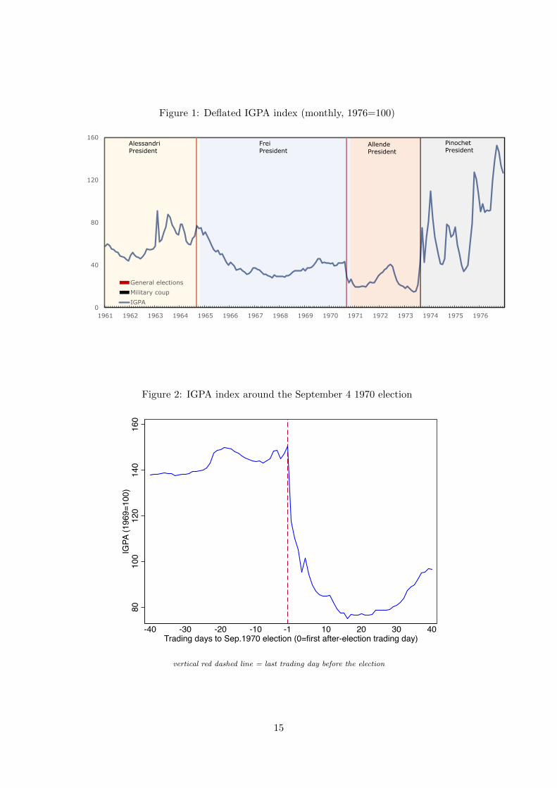
Figure 1: Deflated IGPA index (monthly, 1976=100)

0

1

0

40

80

120

160

1961 1962 1963 1964 1965 1966 1967 1968 1969 1970 1971 1972 1973 1974 1975 1976

General electionsMilitary coupIGPA

AlessandriPresident

FreiPresident

AllendePresident

PinochetPresident

Figure 2: IGPA index around the September 4 1970 election

8010

012

014

016

0IG

PA (1

969=

100)

-40 -30 -20 -10 -1 10 20 30 40Trading days to Sep.1970 election (0=first after-election trading day)

vertical red dashed line = last trading day before the election

15

Figure 3: Monthly real dividends paid by firms listed in Santiago

0

1

0

20

40

60

80

100

120

140

160

180

200

1961 1962 1963 1964 1965 1966 1967 1968 1969 1970 1971 1972 1973 1974 1975 1976

General elections Military coupDividends (Raw Data) Dividends (12-months moving average)

AlessandriPresident

FreiPresident

AllendePresident

PinochetPresident

Figure 4: IGPA index around the September 11 1973 coup

050

010

0015

0020

00IG

PA (1

972=

100)

-40 -30 -20 -10 -1 10 20 30 40Trading days to Sep.1973 coup (0=first after-coup trading day)

vertical red dashed line = last trading day before the coup

16

Figure 5: Empirical distribution of IGPA daily percentage changes (1961-2016, bin width0.10)

1970 election1973 coup

050

010

0015

00Fr

eque

ncy

-20 -10 0 10 20 30 40 50IGPA daily change

(standard deviations from the mean)

17

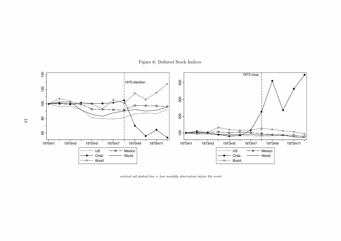
Figure 6: Deflated Stock Indices

1970 election

6080

100

120

140

1970m1 1970m3 1970m5 1970m7 1970m9 1970m11

US MexicoChile WorldBrazil

1973 coup

100

200

300

400

1973m1 1973m3 1973m5 1973m7 1973m9 1973m11

US MexicoChile WorldBrazil

vertical red dashed line = last monthly observation before the event

18

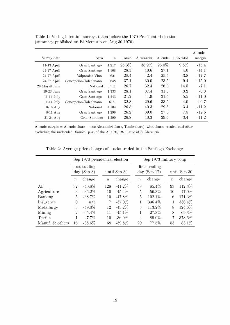
Table 1: Voting intention surveys taken before the 1970 Presidential election(summary published on El Mercurio on Aug 30 1970)

Allende

Survey date Area n Tomic Alessandri Allende Undecided margin

11-13 April Gran Santiago 1,217 26.3% 38.9% 25.0% 9.8% -15.424-27 April Gran Santiago 1,108 28.3 40.6 27.1 4.0 -14.124-27 April Valparaiso-Vina 621 28.4 42.4 25.4 3.8 -17.724-27 April Concepcion-Talcahuano 648 37.1 30.0 23.5 9.4 -15.0

29 May-9 June National 3,711 26.7 32.4 26.3 14.5 -7.119-23 June Gran Santiago 1,333 28.1 37.4 31.3 3.2 -6.311-14 July Gran Santiago 1,243 21.2 41.9 31.5 5.5 -11.011-14 July Concepcion-Talcahuano 676 32.8 29.6 33.5 4.0 +0.78-16 Aug National 4,104 26.8 40.3 29.5 3.4 -11.28-11 Aug Gran Santiago 1,296 26.2 39.0 27.3 7.5 -12.6

21-24 Aug Gran Santiago 1,290 26.8 40.3 29.5 3.4 -11.2

Allende margin = Allende share - max(Alessandri share, Tomic share), with shares recalculated after

excluding the undecided. Source: p.35 of the Aug 30, 1970 issue of El Mercurio

Table 2: Average price changes of stocks traded in the Santiago Exchange

Sep 1970 presidential election Sep 1973 military coup

first trading first tradingday (Sep 8) until Sep 30 day (Sep 17) until Sep 30

n change n change n change n change

All 32 -40.8% 128 -41.2% 48 85.4% 93 112.3%Agriculture 3 -36.2% 10 -45.4% 5 56.3% 10 47.0%Banking 5 -38.7% 10 -47.8% 5 102.1% 6 171.3%Insurance 0 n/a 7 -37.0% 1 336.4% 1 336.4%Metallurgy 5 -49.0% 12 -43.2% 3 113.2% 8 124.6%Mining 2 -65.4% 11 -45.1% 1 27.3% 8 69.3%Textile 1 -7.7% 10 -36.9% 4 89.0% 7 378.6%Manuf. & others 16 -38.6% 68 -39.8% 29 77.5% 53 83.1%

19

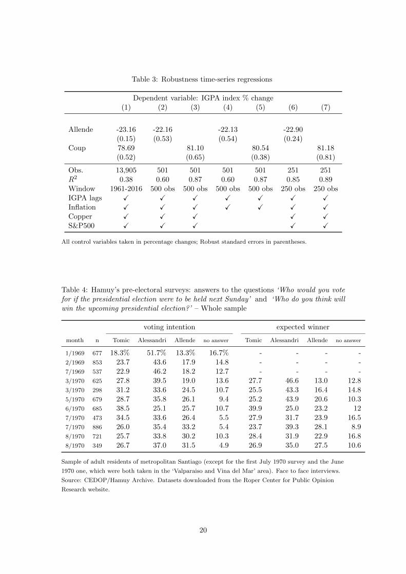
Table 3: Robustness time-series regressions

Dependent variable: IGPA index % change(1) (2) (3) (4) (5) (6) (7)

Allende -23.16 -22.16 -22.13 -22.90(0.15) (0.53) (0.54) (0.24)

Coup 78.69 81.10 80.54 81.18(0.52) (0.65) (0.38) (0.81)

Obs. 13,905 501 501 501 501 251 251R

2 0.38 0.60 0.87 0.60 0.87 0.85 0.89Window 1961-2016 500 obs 500 obs 500 obs 500 obs 250 obs 250 obsIGPA lags X X X X X X XInflation X X X X X X XCopper X X X X XS&P500 X X X X X

All control variables taken in percentage changes; Robust standard errors in parentheses.

Table 4: Hamuy’s pre-electoral surveys: answers to the questions ‘Who would you votefor if the presidential election were to be held next Sunday’ and ‘Who do you think willwin the upcoming presidential election?’ – Whole sample

voting intention expected winner

month n Tomic Alessandri Allende no answer Tomic Alessandri Allende no answer

1/1969 677 18.3% 51.7% 13.3% 16.7% - - - -2/1969 853 23.7 43.6 17.9 14.8 - - - -7/1969 537 22.9 46.2 18.2 12.7 - - - -3/1970 625 27.8 39.5 19.0 13.6 27.7 46.6 13.0 12.83/1970 298 31.2 33.6 24.5 10.7 25.5 43.3 16.4 14.85/1970 679 28.7 35.8 26.1 9.4 25.2 43.9 20.6 10.36/1970 685 38.5 25.1 25.7 10.7 39.9 25.0 23.2 127/1970 473 34.5 33.6 26.4 5.5 27.9 31.7 23.9 16.57/1970 886 26.0 35.4 33.2 5.4 23.7 39.3 28.1 8.98/1970 721 25.7 33.8 30.2 10.3 28.4 31.9 22.9 16.88/1970 349 26.7 37.0 31.5 4.9 26.9 35.0 27.5 10.6

Sample of adult residents of metropolitan Santiago (except for the first July 1970 survey and the June

1970 one, which were both taken in the ‘Valparaiso and Vina del Mar’ area). Face to face interviews.

Source: CEDOP/Hamuy Archive. Datasets downloaded from the Roper Center for Public Opinion

Research website.

20

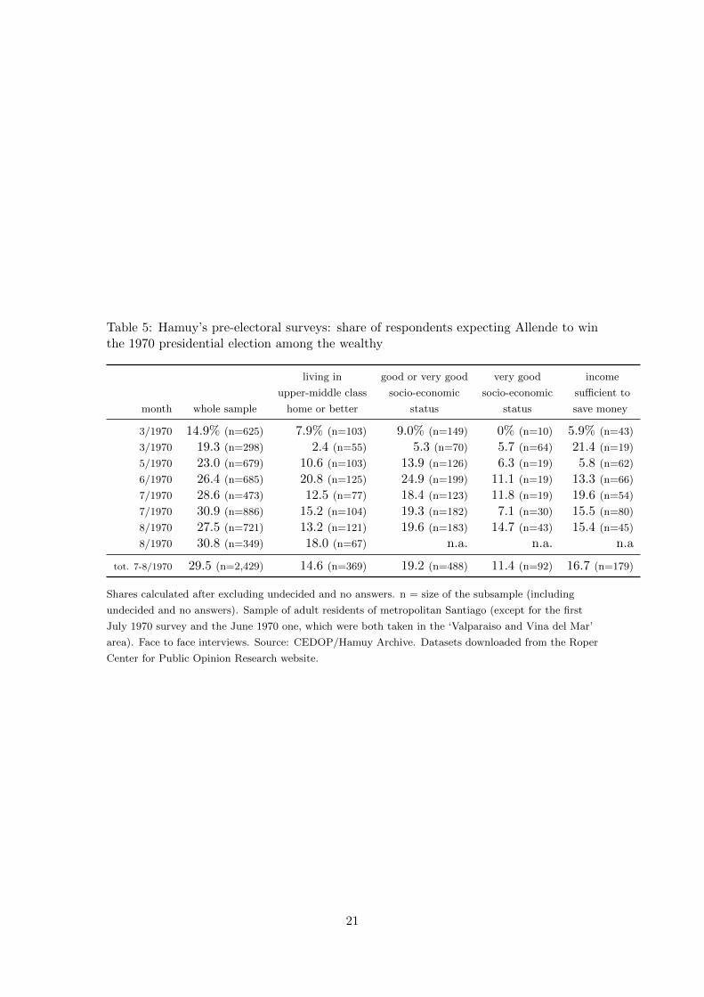
Table 5: Hamuy’s pre-electoral surveys: share of respondents expecting Allende to winthe 1970 presidential election among the wealthy

living in good or very good very good income

upper-middle class socio-economic socio-economic su�cient to

month whole sample home or better status status save money

3/1970 14.9% (n=625) 7.9% (n=103) 9.0% (n=149) 0% (n=10) 5.9% (n=43)

3/1970 19.3 (n=298) 2.4 (n=55) 5.3 (n=70) 5.7 (n=64) 21.4 (n=19)

5/1970 23.0 (n=679) 10.6 (n=103) 13.9 (n=126) 6.3 (n=19) 5.8 (n=62)

6/1970 26.4 (n=685) 20.8 (n=125) 24.9 (n=199) 11.1 (n=19) 13.3 (n=66)

7/1970 28.6 (n=473) 12.5 (n=77) 18.4 (n=123) 11.8 (n=19) 19.6 (n=54)

7/1970 30.9 (n=886) 15.2 (n=104) 19.3 (n=182) 7.1 (n=30) 15.5 (n=80)

8/1970 27.5 (n=721) 13.2 (n=121) 19.6 (n=183) 14.7 (n=43) 15.4 (n=45)

8/1970 30.8 (n=349) 18.0 (n=67) n.a. n.a. n.a

tot. 7-8/1970 29.5 (n=2,429) 14.6 (n=369) 19.2 (n=488) 11.4 (n=92) 16.7 (n=179)

Shares calculated after excluding undecided and no answers. n = size of the subsample (including

undecided and no answers). Sample of adult residents of metropolitan Santiago (except for the first

July 1970 survey and the June 1970 one, which were both taken in the ‘Valparaiso and Vina del Mar’

area). Face to face interviews. Source: CEDOP/Hamuy Archive. Datasets downloaded from the Roper

Center for Public Opinion Research website.

21

Appendix: Voting intention surveys and probability of Al-

lende victory

We have reported voting intentions from Hamuy’s data (Table 4) and from other sur-

veys performed in the months leading to the 1970 election and published by the leading

newspaper El Mercurio (Table 1). Not a single one of the Hamuy surveys has Allende as

the front runner, although he clearly gained ground after his candidacy was confirmed

by the UP in early 1970. Alessandri had announced his candidacy earlier, in 1969 (Navia

and Osorio, 2017, p. 10).1

Concerning the other surveys, out of 11 opinion polls taken between April 1970 and

the election (two at the national level, six taken in the ‘Gran Santiago’ area, two taken

in Concepcion and Talcahuano, one taken in Valparaiso and Vina del Mar), only one

(taken between July 11 and July 14 in Concepcion and Talcahuano) had Allende closely

winning, while 9 (including the two taken at the national level) had Alessandri winning

and 1 predicted a Tomic victory. The last national poll taken before the election indi-

cated a 11.1% margin between Alessandri and Allende.

It is interesting to ask if the voting intention surveys in Table 1 (conducted inde-

pendently of those of Hamuy, as far as we know) imply an ex-ante perceived probability

of Allende victory broadly consistent with Hamuy’s expectation surveys data (in which,

in the overall population, 30% of responders expected an Allende victory). Of course

this calculation requires some rule for inferring probabilities of victory from voting in-

tentions, which is not straightforward. To provide a rough calculation, we use data from

surveys and prediction markets concerning the 2000 Mexican presidential election to

infer a relation between margins in voting intentions and probabilities of victory, and

then apply this relation to the data in Table 1.

The Mexican electoral system can be considered analogous to the one holding in

1Figure 1 in Navia and Osorio (2017, p. 11) appears to suggest that Allende suddenly gained asubstantial lead in Hamuy’s second August 1970 survey. This is not what is found in the Hamuy surveysas available at the Roper Center website (which is also the source cited by their article). We believethat this is a mistake caused by the fact that, as of August 10 2017 (when we last accessed the website),the ASCII version of the dataset available in the Roper Center website appeared to be mistaken, giventhat results, number of observations and number of options for each question did not coincide with themetadata and with the original documents reporting results (which the Roper Center also provides inscanned PDF format). The SPSS version of the dataset, instead, appears consistent with the metadataand the PDFs, and it contains the figures that we have reported in Table 4.

22

Chile in 1970: the president is elected in a multi-candidate election and a plurality of

votes is su�cient to win the presidency.2 Besides the electoral system, the 2000 Mexican

election also shares other similarities with the Chilean 1970 election: three candidates

received more than 10% of the vote each, the election was won by an opposition party

which had never been in power before, and the outcome was largely a surprise. The

Iowa Electronic Markets (IEM – one of the most popular prediction markets) provides

data on implied probabilities of victory for the 2000 election in Mexico.3 We match

the IEM data with data on voting intentions from the Mexico 2000 Panel Study (as

reported in Klesner, 2005) to infer a relation between shares in voting intention surveys

and probabilities of victory.

According to the Mexico 2000 Panel Study, as of June (the election was held on

July 2), 35% of respondents supported the incumbent PRI, 23% the PAN (who would

eventually win the election) and 10% the PRD, while the remaining 32% of respondents

supported none or were undecided. The margin between the PRI and the PAN can-

didates (after excluding the undecided) was 17.6%. The probability of a PAN victory

implied by the IEM prediction market before the election was around 27%, while the

probability of a PRI victory was around 73%. The ratio between the margin in perceived

probabilities and in voting intention shares was therefore 2.6. If we apply the same ratio

to the Chile 1970 election, the implied probability of an Allende victory would be 26%.

Reassuringly, this figure is quite near to the share of responders expecting an Allende

victory in the Hamuy’s vote expectation surveys which we use as our main source (30%).

References

Klesner, J.L. (2005). “Electoral Competition and the New Party System in Mexico”.

In: Latin American Politics and Society 47.2, pp. 103–142. doi: 10.1111/j.1548-

2456.2005.tb00311.x.2The US system, on which prediction markets data is most abundant, is substantially di↵erent,

because of the role of the electoral college, and because of the consolidated two-party system, whichgenerates races with only two competitive candidates.

3The 2000 election is the only Mexican presidential election covered by the IEM so far.

23

Navia, P. and R. Osorio (2017). “Make the Economy Scream? Economic, Ideological and

Social Determinants of Support for Salvador Allende in Chile, 19703”. In: Journal

of Latin American Studies, 127. doi: 10.1017/S0022216X17000037.

24