Embed Size (px)
Citation preview
DEPARTMENT OF ECONOMICS
Working Paper
UNIVERSITY OF MASSACHUSETTS AMHERST
Bandwagon, underdog, and political competition: The uni-dimensional case
by
Woojin Lee
Working Paper 2008-07 Revised version
1
Bandwagon, underdog, and political competition:
The uni-dimensional case
April 18, 2008
[First version: February 28, 2008]
Woojin Lee
Department of Economics
University of Massachusetts
Amherst, MA 01002
I thank John Roemer for his comments, which improved the paper significantly.
2
Abstract
The present paper studies the effects of bandwagon and underdog on the political
equilibrium of two-party competition models. We adapt the generalized Wittman-Roemer model
of political competition for voter conformism, which views political competition as the one
between parties with factions of the opportunists and the militants that Nash-bargain one another,
and consider three special cases of the general model: the Hotelling-Downs model, the classical
Wittman-Roemer model, and what we call the ideological-party model.
In the Hotelling-Downs model, where the militants have no bargaining power in both
parties, political parties put forth an identical policy at the equilibrium, regardless of the type of
voter conformism, and this is the only equilibrium. Thus neither bandwagon nor underdog has
any effect on the Hotelling-Downs political equilibrium.
In both the ideological-party and classical Wittman-Roemer models, parties propose
differentiated policies at the equilibrium, and the extent of policy differentiation depends on the
degree of voter conformism. In these models, multiple equilibria generically exist when the
bandwagon effect is sufficiently strong. We characterize the relationship between the extent of
voter conformism and equilibrium party platforms in dynamically stable equilibria of these
models.
JEL Categories: D3, D7, H2
Keywords: bandwagon, underdog, Nash-bargaining, Hotelling-Downs model, Wittman-
Roemer model, ideological-party model
1
1. Introduction
In almost all democracies, opinion polls have become an integral part of national elections.
Public opinion polls provide aggregate information to the public about the views of their fellow
citizens. By doing so, they may sometimes influence the behavior of voters and thus who will be
elected. In turn, opinion polls may influence announced policies of candidates as well.
The various theories about how this happens can be divided into three categories: ‘voter
conformism,’ ‘strategic voting,’ and ‘participation/abstention.’
A well-known example of voter conformism is the bandwagon effect. The bandwagon
effect occurs when the poll prompts voters to back the candidate shown to be winning in the poll,
thus increasing his/her chances of being on the winner’s side in the end. The idea that voters are
susceptible to such an effect is old, and has remained persistent in spite of much debate on its
empirical existence. Bartels (1985, 1988), for instance, shows that voters are motivated in part by
a desire to vote for the winning candidate. The opposite of the bandwagon effect is the underdog
effect; this occurs when people support, out of sympathy, the candidate perceived to be ‘losing’
the elections. In a meta-study of research on this topic, Irwin and van Holsteyn (2002) show that
from the 1980s onward, empirical evidence for the existence of the bandwagon effect is found
more often than for the underdog effect.1
1 There have been at least two explanations for the existence of voter conformism. The first consists in assuming that
polls may exert a normative influence over voters; when voters perceive the existence of a social norm – defined by a
majority preference expressed in polls in the case of a bandwagon effect – they may feel compelled to abandon their
views and comply with such norms, to avoid perhaps cognitive dissonance. The second, which seems more
compelling, consists in assuming that individuals may be influenced by polls because they use revealed public
preferences as information about the correct option to take. Considering they have strong incentives to minimize the
2
The second category of theories on the effect of polls on voting concerns strategic voting.
These theories are based on the idea that voters will sometimes not choose the candidate they
prefer the most, but another, less-preferred, candidate from strategic considerations. An example
can be found in the UK general election of 1997. Then Cabinet Minister, Michael Portillo's
constituency of Enfield was believed to be a safe seat, but opinion polls showed that the Labour
candidate Stephen Twigg was steadily gaining support, which may have prompted supporters of
other parties to vote for Twigg in order to remove Portillo.
The third category of theories concerns voter participation/abstention. It is often
suggested that supporters of the candidate shown to be significantly lagging behind may give up
casting their ballots, resulting in a landslide victory of another candidate. In the South Korean
presidential election of 2007, when a conservative candidate, M.B. Lee, achieved a landslide
victory over a liberal candidate, D.Y. Chung, with the vote shares of 48.7% versus 26.1%, it was
widely believed that anti-Lee voters had abstained significantly, concluding from several pre-
election polls that Chung would have no chance of winning even if they would cast votes for him.
(Indeed the voting rate was 63%, the lowest one since 1987.) But the opposite of this
phenomenon may happen as well. A well-known example is the boomerang effect where the
likely supporters of the candidate shown to be winning feel that they are ‘home and dry’ and that
their vote is not required, thus allowing another candidate to win.
Since Leibenstein’s (1950) pioneering work on consumer conformism, there have been
many studies on the effect of conformism on economic behavior; see Akerlof (1997), Banerjee
(1992), Bernheim (1994), Birkchandani et al. (1992), and Schelling (1974). There are also some
costs of acquiring the information necessary to make right choices (Downs, 1957), voters may rely upon ‘information
shortcuts,’ such as group references, party identification, or knowledge about where other voters stand on issues.
3
political models incorporating the effect of opinion polls on voter conformism and its
consequence for actual vote shares (Aldrich, 1980; Baumol, 1957; Simon, 1954). To the best of
our knowledge, no political models have been developed to study the effect of voter conformism
on the nature of political competition. The current paper aims at filling this gap in the literature.
In the present paper, we are particularly interested in the effect of voter conformism, in the form
of bandwagon or underdog, on equilibrium party platforms.
We ask the following: Does the presence of voter conformism affect the policy positions
of candidates? If it does, does it mitigate policy differentiation among candidates, or exacerbate
it?
To answer these questions, we adapt the generalized Wittman-Roemer model of two-party
competition for voter conformism. Instead of viewing political competition as occurring between
two parties each of which is a unitary actor that maximizes a certain payoff function, the
generalized Wittman-Roemer model views political equilibrium as the one obtained from
competition between parties with factions that have different goals and Nash-bargain with one
another to set the policy. Following Roemer (2001), we assume that there are two factions in each
party: the opportunists whose goal is to win the election and the militants whose objective is to
maximize the average well-being of their party members. 2
The generalized Wittman-Roemer model has one advantage for our study; it covers
various models of political competition as its special cases. Thus it allows us to study the
consequence of voter conformism on the equilibrium of various political models in a unified
framework. We will study three special cases of the generalized Wittman-Roemer model of
2 A generalized Wittman-Roemer equilibrium, where bargaining power is fixed, can be considered a special case of
Roemer’s (2001) party unanimity Nash equilibrium, where bargaining power is not specified a priori.
4
political competition, which have received much attention among students of political economy.
One is the Hotelling-Downs model in which parties maximize their probabilities of victory, and
another is the classical Wittman-Roemer model (Roemer, 1997) in which parties maximize the
expected utilities of their key constituents. The third is the one, which we call the ideological-
party model, in which each party sets its policy equal to the ideal tax rate of its endogenously-
determined average member.
In defining voter conformism, we follow Simon (1954). Simon (1954) holds that voting
behavior is a function of voters’ expectations of the electoral outcome, and published poll data
influence these expectations. The bandwagon effect exists if voters are more likely to vote for a
candidate when they expect him to win than when they expect him to lose; if the opposite holds,
the underdog effect exists.
We will define the generalized Wittman-Roemer model’s equilibrium as a static concept,
but the issues we are studying – bandwagon, underdog, and policy positions of candidates – are
inherently dynamic. We show that the model’s equilibrium is identical to a stationary point of a
certain best-response dynamic, and study some of its dynamic properties as well.
Section 2 presents the generalized Wittman-Roemer model of political competition, which
is adapted for voter conformism. Section 3 studies the effect of voter conformism on the
Hotelling-Downs political equilibrium, where the militants have no bargaining power in both
parties. We prove that voter conformism has no effect on the equilibrium policy in this case, for
the unique equilibrium in this model is both parties’ putting forth the same policy. In section 4 we
study another extreme case of the generalized Wittman-Roemer model in which the opportunists
have no bargaining power in both parties: the ideological-party model. In contrast with the
Hotelling-Downs model, the presence of multiple equilibria is generic in this model when the
5
bandwagon effect is sufficiently strong. In those equilibria that are dynamically stable and have
the membership share of party L greater than 0.5 (less than 0.5), an increasing bandwagon effect
decreases (increases) the equilibrium tax rates of both parties; the opposite holds for the underdog
effect. Section 5 studies the classical Wittman-Roemer model in which both the militants and the
opportunists have equal bargaining power in both parties. Two parties in the classical Wittman-
Roemer model propose differentiated equilibrium policies (as in the model without voter
conformism), and the extent of such policy differentiation depends on the degree of voter
conformism. As in the ideological-party model studied in section 4, multiple equilibria
generically exist in the classical Wittman-Roemer model when the bandwagon effect is
sufficiently strong. In contrast with the purely ideological parties, the Wittman-Roemer parties
move in an opposite direction as the parameter capturing the extent of voter conformism increases.
In those Wittman-Roemer equilibria that are dynamically stable, an increasing bandwagon effect
exacerbates the policy differentiation of the two parties; the opposite holds when the underdog
effect is considered. Section 6 concludes. We collect all the proofs in Appendix.
2. The model
Throughout the paper, we will maintain that there are two political parties (or candidates
representing them), L and R, and that the policy space is the unit interval: [0,1]T = . A generic
element of T will be denoted by t , which we call a tax rate, or simply a policy. We assume that
the party that wins the election implements its announced policy. Because we study the models
with two parties, the issue of strategic voting is not our concern. Also the potential issue of voter
participation/abstention is not explicitly modeled.
6
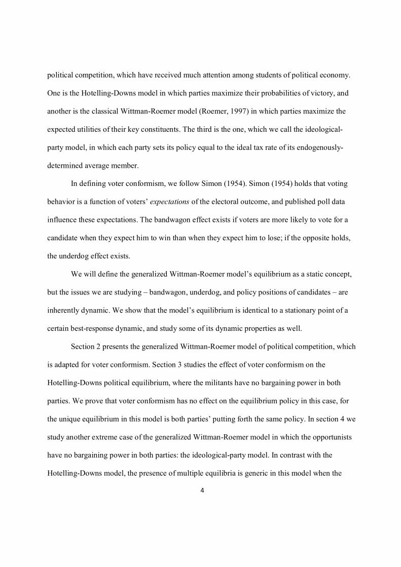
There is a continuum of voters; we are modeling an election in large polities, where no
individual voter is noticeable. Voters are endowed with one-dimensional characteristic, w+
Î R ,
whose distribution is given by a strictly increasing and continuous distribution function (.)F ; its
associated probability measure is denoted by (.)P .3 We call w an income. The mean of w ,
denoted by m , is assumed to exist.
In this model, party membership will be endogenously determined. We assume a perfectly
representative democracy where: (1) every voter belongs to one and only one party (thus there are
no ‘undecided’ voters); (2) each party member receives an equal weight in the determination of
the party’s von Neumann-Morgenstern utility function; and (3) each voter votes for the party of
which he/she is a member.
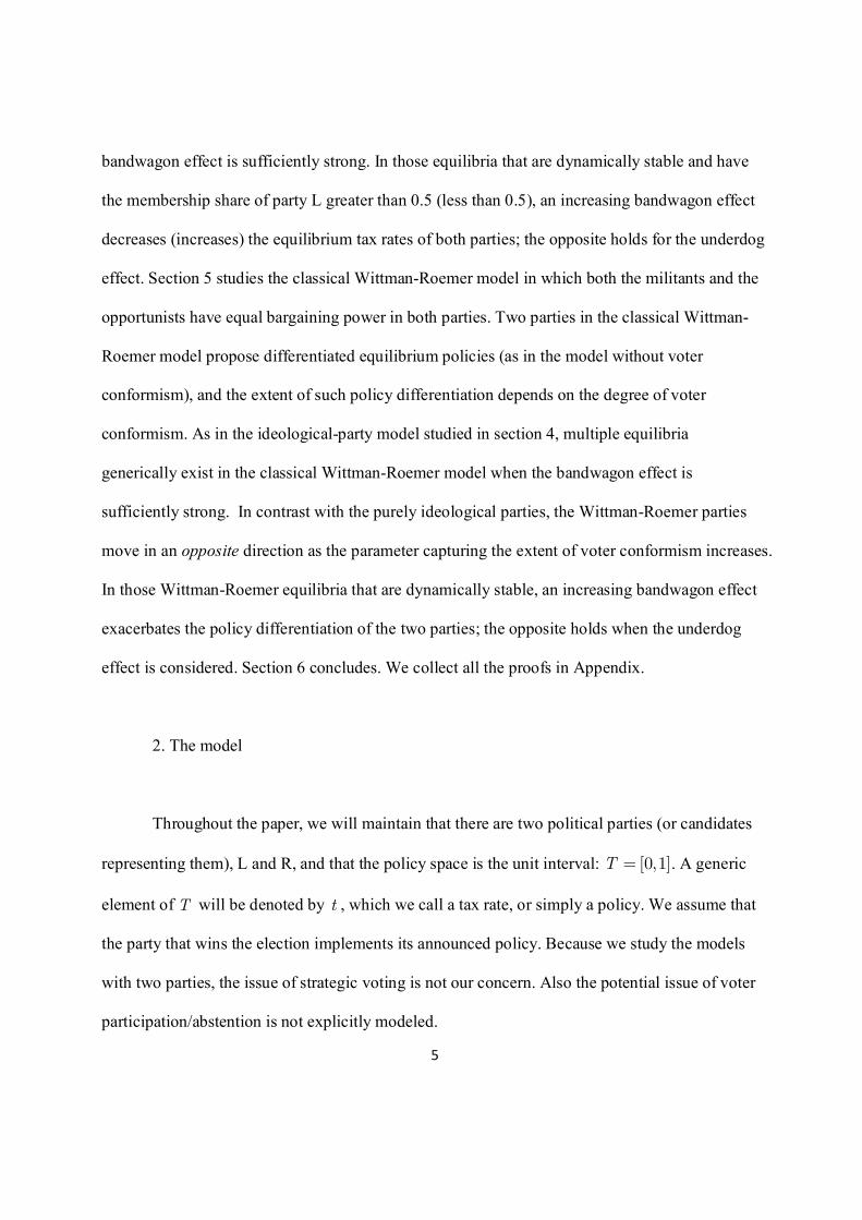
Suppose ( , )L Rt t T TÎ ´ is a pair of policy positions of the two parties and [0,1]x Î is an
expected membership share of party L, which is ascertained perhaps through opinion polls.
(Because there are only two parties, the expected membership share for party R is 1 x- .) Given
( , )j jt x , where L,Rj = , we assume that voter preferences are given by
(1 ) ( ) ( )j j jt w h t xa m qf- + + , (1)
where a is a positive constant, and (.)h and (.)f are functions satisfying the following
conditions.
Assumption 1: (1) : [0,1]f ® R is strictly increasing and finite-valued on [0,1]; and
(2) :h T ® R is strictly increasing, strictly concave, and finite-valued on T.
3 R+ is defined to be the set of all non-negative real numbers, not just of positive numbers.
7
Some remarks are in order regarding voter preferences.
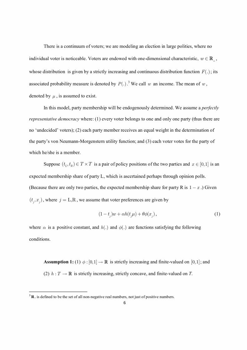
First, facing an election, voters care not only about the policy positions of political parties
but also the membership shares of the parties. Note that the voter’s utility function consists of two
parts: a quasi-linear utility function that represents the economic interests of voters,
(1 ) ( )j jt w h ta m- + , and a utility bonus/penalty from supporting the winning/losing party,
( )jxqf , where L,Rj = . Because (.)f is increasing, we have ( ) (1 )x xqf qf> - if and only if
12
( ) 0xq - > . Thus the bandwagon effect is captured by the assumption that q is positive; other
things being equal, voters prefer a party whose expected membership share is greater than ½. The
presence of the underdog effect would be equivalent to assuming that q is negative. Finally, if
q = 0 , there is no voter conformism.
Second, if we interpret tm as the per capita amount of public goods,4 then a measures the
extent to which voters value the consumption of public goods. The parameter q , on the other
hand, measures the relative salience of voter conformism. By letting a and q vary across voters,
one might allow a voter to be equipped with three characteristics: ( , , )w a q . Our equilibrium will
be well-defined even in that case.5 For the sake of simplicity, we will maintain that the parameter
values of a and q are identical for all voters; voters differ only in the level of incomes that they
hold. Of course, this is a great simplification. If some voters are vulnerable to the bandwagon
effect, others may be susceptible to the underdog effect; still others may receive no influence at
all. Because we do not know who are more susceptible to which effect, we study each case
separately by assuming that all voters are susceptible to the same effect.
4 This is the case if there is no incentive effect of taxation.
5 What is essential in our model is the uni-dimensionality of the policy space, not the uni-dimensionality of the voter
characteristic space.
8
Facing ( , , )L Rt t x , voter w (weakly) prefers L to R if
( ) ( ( ) ( )) ( ( ) (1 )) 0L R L Rt t w h t h t x xa m m q f f- - + - + - - ³ . (2)
If L Rt t> , the left-hand side expression of (2) is decreasing in w and goes to -¥ as w ® ¥ ,
but may be negative at 0w = if 12
( ) 0xq - < . If L Rt t< , it is increasing in w and goes to ¥ as
w ® ¥ , but may be positive at 0w = if 12
( ) 0xq - > .
Thus, for L Rt t¹ , we define the cutoff level of income for inequality (2) as:
( , , ) max[ ( , , ), 0]L R L R
w t t x t t xvº , (3)
where ( ) ( ) ( ) (1 )
( , , ) L RL R
L R L R
h t h t x xt t x
t t t t
m m f fv a q
- - -= +
- -.
By Assumption 1, the first term inside the max expression of equation (3) is always finite
(for L Rt t¹ ). It is not always positive; it can be negative if 1
2( )( ) 0
L Rx t tq - - < . To prevent
uninteresting situations in which ( ) (1 )
L R
x x
t t
f fq
- -
- always dominates
( ) ( )L R
L R
h t h t
t t
m ma
-
-, we
make the following assumption; without this assumption, there may exist some [0,1]x Î at which
one party is preferred by ‘all’ voters for all distinct pairs of L Rt t¹ .
Assumption 2: For any [0,1]x Î , there exists at least one pair of distinct policies ( , )L Rt t ,
L Rt t¹ , such that ( , , ) 0
L Rw t t x > .
9
The set of voters who prefer L to R is the set of w for whom inequality (2) is satisfied.
Thus, given ( , , )L Rt t x , the set of voters who prefer L to R is
12
12
12
{ | ( , , )} if
{ | ( , , )} if
if and ( ) 0( , , )
a random half subset of if and ( ) 0
if and ( ) 0,
L R L R
L R L R
L RL R
L R
L R
w w w t t x t t
w w w t t x t t
t t xt t x
t t x
t t x
q
q
q
+
+
+
+
ìï Î £ >ïïï Î ³ <ïïïï = - >W =í
= - =
Æ = - <î
R
R
R
Rïïïïïïïï
(4)
and the actual membership share of party L is given by
' ( ( , , ))L R
x P t t x= W , (5)
where
( )( )
12
1 12 2
12
( , , ) if
1 ( , , ) if
( ( , , )) 1 if and ( ) 0
if and ( ) 0
0 if and ( ) 0.
L R L R
L R L R
L R L R
L R
L R
F w t t x t t
F w t t x t t
P t t x t t x
t t x
t t x
q
q
q
ìï >ïïï - <ïïïïW = = - >íïï = - =ïïïï = - <ïïî
Note a difference between the case in which 12
and ( ) 0L Rt t xq= - > and the case in
which 12
and ( ) 0L Rt t xq= - = . In the former case, all voters strictly prefer L to R, while in the
latter case, voters are indifferent between them. We assume that indifferent voters decide their
party membership by flipping a fair coin. This also means that the two random half-subsets of
+R will have exactly the same distributions of voters as (.)F .
So far, we described the basic data of the model. We now introduce the two factions that
Nash-bargain one another in setting the party policy.
The opportunists in each party are those who advocate a policy that maximizes an
increasing function of its actual membership share. To be precise, let : [0,1] [0,1]F ® be an
10
increasing function such that 1 12 2
( ) and ( ) 1 (1 )x xF = F = -F - . Then, given ( , , )L Rt t x , party
L’s opportunists are maximizing
( )( , ; ) ( ( , , ))L R L Rt t x P t t xp = F W , (6)
and party’s R’s opportunists are maximizing ( )1 ( ( , , )) 1 ( , ; )L R L R
P t t x t t xpF - W = - .
Our formulation of the objective function of the opportunists covers a number of different
specifications in the literature on political economy.
First, it covers the models with electoral uncertainty, where ( , , )L Rt t xp and
1 ( , , )L Rt t xp- are interpreted as probabilities of victory. To see this, suppose the actual vote
share for L is given by ( ( , , ))L R
P t t x eW + , where e is a random variable distributed by a
symmetric distribution function (.)G such that 12
(0)G = . Then party L’s probability of victory is
( )Pr( ( ( , , )) 0.5) 1 0.5 ( ( , , ))L R L R
P t t x G P t t xeW + > = - - W , and thus ( ) ( 0.5)x G xF = - .
Second, if 1 12 2
12( ,1] { }
( ) 1 ( ) 1 ( )x x xF = + , where 1 ( )Ax is an indicator function that takes 1 if
x AÎ and 0 otherwise, then ( , , )L Rt t xp can be considered a probability of victory in the models
with electoral certainty.
Third, if ( )x xF = , then ( , , )L Rt t xp and 1 ( , , )
L Rt t xp- are actual membership shares.
This might be the case if there is no electoral uncertainty and the election is not of the winner-
takes-all type. For instance, under proportional representation, the opportunists may care more
about vote shares than probabilities of victory. 6
6 Baron (1993) and Ortuno-Ortin (1997) study models of political competition under proportional representation, in
which the influence of the groups favoring a certain policy is proportional to the percentage votes favoring that policy.
11
Although our formulation is flexible enough to cover various specifications, we will call
( , , )L Rt t xp and 1 ( , , )
L Rt t xp- probabilities of victory throughout the paper. Also we will
maintain the following assumption.
Assumption 3: : [0,1] [0,1]F ® is strictly increasing.7
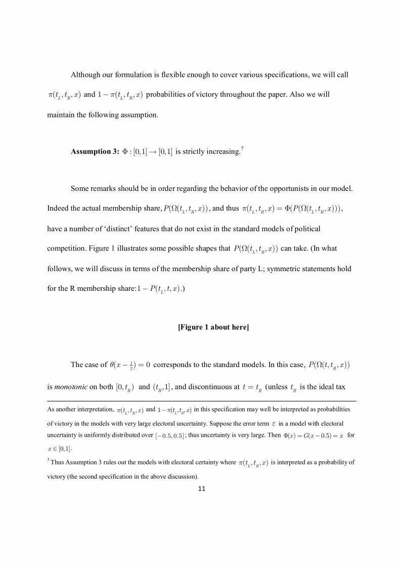
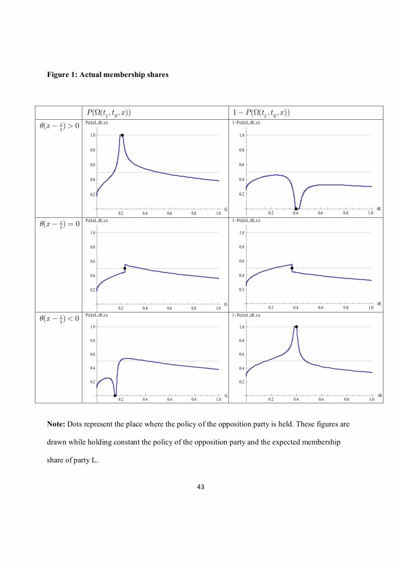
Some remarks should be in order regarding the behavior of the opportunists in our model.
Indeed the actual membership share, ( ( , , ))L R
P t t xW , and thus ( , , ) ( ( ( , , )))L R L Rt t x P t t xp = F W ,
have a number of ‘distinct’ features that do not exist in the standard models of political
competition. Figure 1 illustrates some possible shapes that ( ( , , ))L R
P t t xW can take. (In what
follows, we will discuss in terms of the membership share of party L; symmetric statements hold
for the R membership share:1 ( , , )L
P t t x- .)
[Figure 1 about here]
The case of 12
( ) 0xq - = corresponds to the standard models. In this case, ( ( , , ))R
P t t xW
is monotonic on both [0, )Rt and ( ,1]
Rt , and discontinuous at
Rt t= (unless
Rt is the ideal tax
As another interpretation, ( , , )
L Rt t xp and 1 ( , , )
L Rt t xp- in this specification may well be interpreted as probabilities
of victory in the models with very large electoral uncertainty. Suppose the error term e in a model with electoral
uncertainty is uniformly distributed over [ 0.5, 0.5]- ; thus uncertainty is very large. Then ( ) ( 0.5)x G x xF = - = for
[0,1]x Î .
7 Thus Assumption 3 rules out the models with electoral certainty where ( , , )L Rt t xp is interpreted as a probability of
victory (the second specification in the above discussion).
12
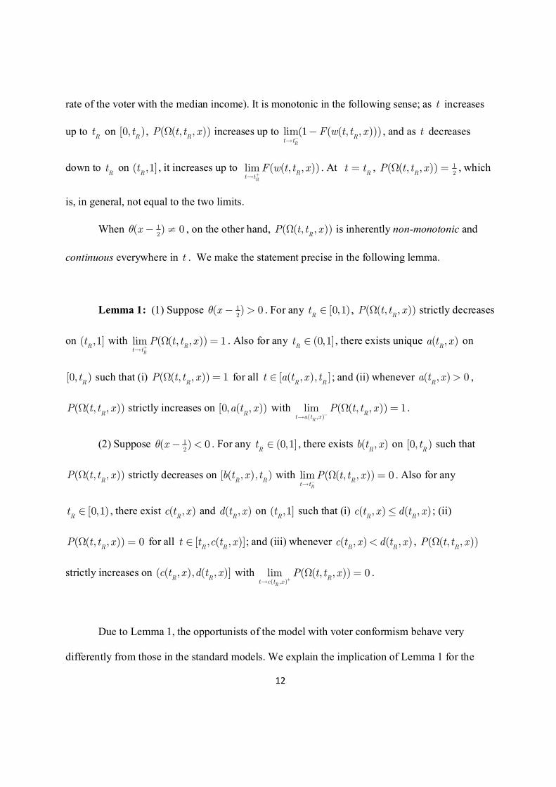
rate of the voter with the median income). It is monotonic in the following sense; as t increases
up to Rt on [0, )
Rt , ( ( , , ))
RP t t xW increases up to lim(1 ( ( , , )))
R
Rt t
F w t t x-®
- , and as t decreases
down to Rt on ( ,1]
Rt , it increases up to lim ( ( , , ))
R
Rt t
F w t t x+®
. At R
t t= , 12
( ( , , ))R
P t t xW = , which
is, in general, not equal to the two limits.
When 12
( ) 0xq - ¹ , on the other hand, ( ( , , ))R
P t t xW is inherently non-monotonic and
continuous everywhere in t . We make the statement precise in the following lemma.
Lemma 1: (1) Suppose 12
( ) 0xq - > . For any [0,1)Rt Î , ( ( , , ))
RP t t xW strictly decreases
on ( ,1]Rt with lim ( ( , , )) 1
R
Rt t
P t t x+®
W = . Also for any (0,1]Rt Î , there exists unique ( , )
Ra t x on
[0, )Rt such that (i) ( ( , , )) 1
RP t t xW = for all [ ( , ), ]
R Rt a t x tÎ ; and (ii) whenever ( , ) 0
Ra t x > ,
( ( , , ))R
P t t xW strictly increases on [0, ( , ))R
a t x with ( , )
lim ( ( , , )) 1R
Rt a t x
P t t x-®
W = .
(2) Suppose 12
( ) 0xq - < . For any (0,1]Rt Î , there exists ( , )
Rb t x on [0, )
Rt such that
( ( , , ))R
P t t xW strictly decreases on [ ( , ), )R R
b t x t with lim ( ( , , )) 0R
Rt t
P t t x-®
W = . Also for any
[0,1)Rt Î , there exist ( , )
Rc t x and ( , )
Rd t x on ( ,1]
Rt such that (i) ( , ) ( , )
R Rc t x d t x£ ; (ii)
( ( , , )) 0R
P t t xW = for all [ , ( , )]R R
t t c t xÎ ; and (iii) whenever ( , ) ( , )R R
c t x d t x< , ( ( , , ))R
P t t xW
strictly increases on ( ( , ), ( , )]R R
c t x d t x with ( , )lim ( ( , , )) 0
R
Rt c t x
P t t x+®
W = .
Due to Lemma 1, the opportunists of the model with voter conformism behave very
differently from those in the standard models. We explain the implication of Lemma 1 for the
13
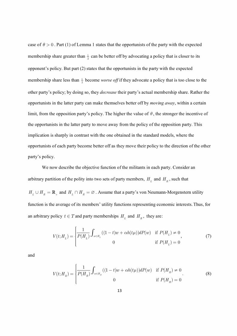
case of 0q > . Part (1) of Lemma 1 states that the opportunists of the party with the expected
membership share greater than 12
can be better off by advocating a policy that is closer to its
opponent’s policy. But part (2) states that the opportunists in the party with the expected
membership share less than 12
become worse off if they advocate a policy that is too close to the
other party’s policy; by doing so, they decrease their party’s actual membership share. Rather the
opportunists in the latter party can make themselves better off by moving away, within a certain
limit, from the opposition party’s policy. The higher the value of q , the stronger the incentive of
the opportunists in the latter party to move away from the policy of the opposition party. This
implication is sharply in contrast with the one obtained in the standard models, where the
opportunists of each party become better off as they move their policy to the direction of the other
party’s policy.
We now describe the objective function of the militants in each party. Consider an
arbitrary partition of the polity into two sets of party members, L
H and R
H , such that
L RH H
+È = R and
L RH HÇ = Æ . Assume that a party’s von Neumann-Morgenstern utility
function is the average of its members’ utility functions representing economic interests. Thus, for
an arbitrary policy t TÎ and party memberships L
H and R
H , they are:
1((1 ) ( )) ( ) if ( ) 0
( )( ; )
0 if ( ) 0
LL
w HLL
L
t w h t dP w P HP HV t H
P H
a mÎ
ìïï - + ¹ïï= íïï =ïïî
ò , (7)
and
1((1 ) ( )) ( ) if ( ) 0
( )( ; )
0 if ( ) 0
RR
w HRR
R
t w h t dP w P HP HV t H
P H
a mÎ
ìïï - + ¹ïï= íïï =ïïî
ò . (8)
14
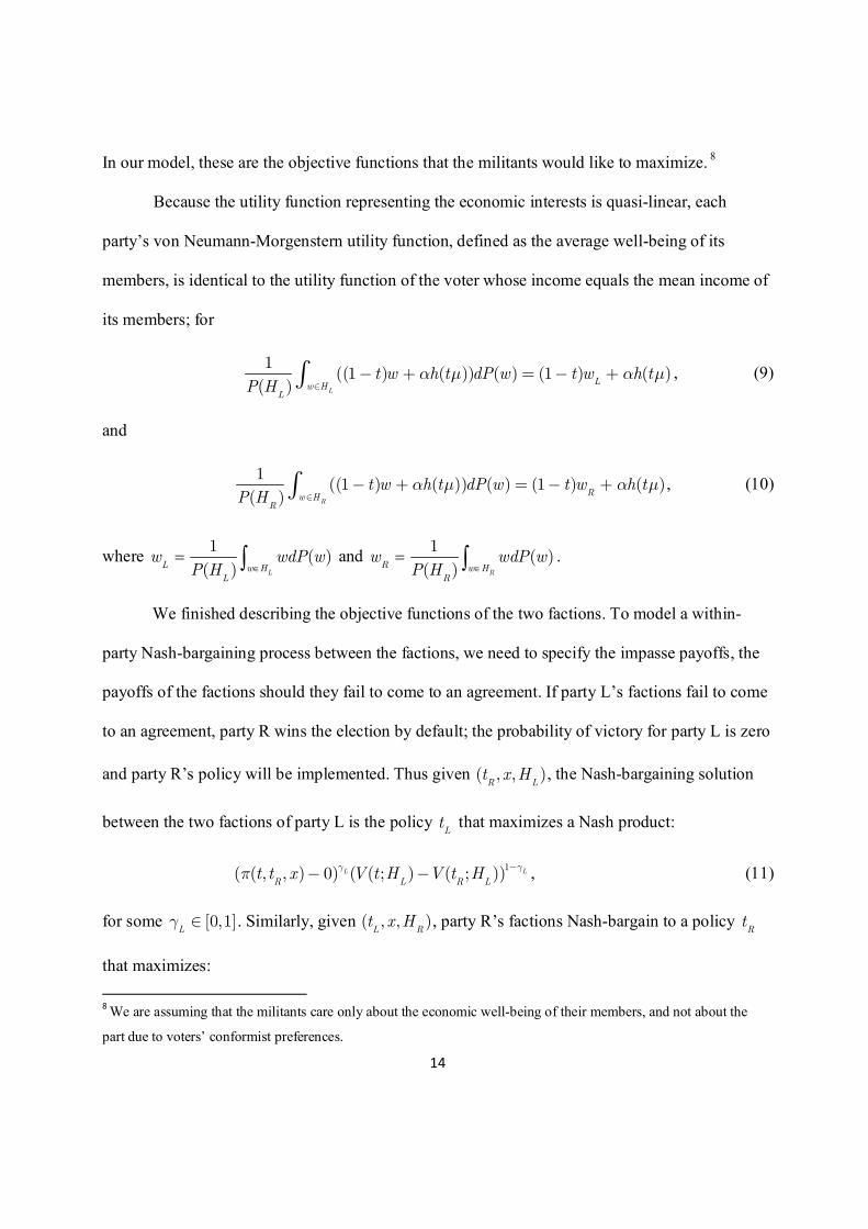
In our model, these are the objective functions that the militants would like to maximize. 8
Because the utility function representing the economic interests is quasi-linear, each
party’s von Neumann-Morgenstern utility function, defined as the average well-being of its
members, is identical to the utility function of the voter whose income equals the mean income of
its members; for
1((1 ) ( )) ( ) (1 ) ( )
( ) LL
w HL
t w h t dP w t w h tP H
a m a mÎ
- + = - +ò , (9)
and
1((1 ) ( )) ( ) (1 ) ( )
( ) RRw H
R
t w h t dP w t w h tP H
a m a mÎ
- + = - +ò , (10)
where 1
( )( ) L
L w HL
w wdP wP H Î
= ò and 1
( )( ) R
R w HR
w wdP wP H Î
= ò .
We finished describing the objective functions of the two factions. To model a within-
party Nash-bargaining process between the factions, we need to specify the impasse payoffs, the
payoffs of the factions should they fail to come to an agreement. If party L’s factions fail to come
to an agreement, party R wins the election by default; the probability of victory for party L is zero
and party R’s policy will be implemented. Thus given ( , , )R Lt x H , the Nash-bargaining solution
between the two factions of party L is the policy Lt that maximizes a Nash product:
1( ( , , ) 0) ( ( ; ) ( ; ))L L
R L R Lt t x V t H V t H
g gp
-- - , (11)
for some [0,1]L
g Î . Similarly, given ( , , )L Rt x H , party R’s factions Nash-bargain to a policy
Rt
that maximizes:
8 We are assuming that the militants care only about the economic well-being of their members, and not about the
part due to voters’ conformist preferences.
15
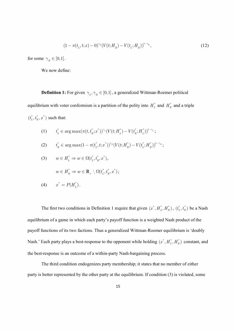
1(1 ( , ; ) 0) ( ( ; ) ( ; )) ,R R
L R L Rt t x V t H V t H
g gp
-- - - (12)
for some [0,1]R
g Î .
We now define:
Definition 1: For given , [0,1]L R
g g Î , a generalized Wittman-Roemer political
equilibrium with voter conformism is a partition of the polity into *LH and *
RH and a triple
* * *( , , )L Rt t x such that:
(1) 1* * * * * *arg max( ( , ; )) ( ( ; ) ( ; ))L L
L R L R Lt t t x V t H V t H
g gp
-Î - ;
(2) 1* * * * * *arg max(1 ( , ; )) ( ( ; ) ( ; ))R R
R L R L Rt t t x V t H V t H
g gp
-Î - - ;
(3) * * * *( , , )L L R
w H w t t xÎ Þ Î W ,
* * * *\ ( , , )R L R
w H w t t x+
Î Þ Î WR ;
(4) * *( )L
x P H= .
The first two conditions in Definition 1 require that given * * *( , , )L Rx H H , * *( , )L Rt t be a Nash
equilibrium of a game in which each party’s payoff function is a weighted Nash product of the
payoff functions of its two factions. Thus a generalized Wittman-Roemer equilibrium is ‘doubly
Nash.’ Each party plays a best-response to the opponent while holding * * *( , , )L Rx H H constant, and
the best-response is an outcome of a within-party Nash-bargaining process.
The third condition endogenizes party membership; it states that no member of either
party is better represented by the other party at the equilibrium. If condition (3) is violated, some
16
members of party j will prefer to join party i . This is certainly not a stable situation. Baron
(1993) first uses the idea here – that malcontents ‘vote with their feet’ by defecting to the other
party – in the context of political competition, although our formulation is close to those of
Ortuno-Ortin and Roemer (1998) and Roemer (2001: page 92).
The fourth condition requires that the actual party membership shares be identical to the
expected party membership shares at the equilibrium party platforms. Thus a generalized
Wittman-Roemer equilibrium with voter conformism is a rational-expectation equilibrium. One
needs to note that the fourth condition is weaker than the requirement that the actual party
membership shares be identical to the expected party membership shares for all possible pairs of
party platforms; it requires only that they are identical at the equilibrium platforms. Another
interpretation of the fourth condition is that polls are accurate in predicting party membership
shares at the equilibrium party platforms.
There emerge several interesting special cases from a generalized Wittman-Roemer
political equilibrium with voter conformism.
First, if we set 1L R
g g= = , we have the Hotelling-Downs model, adapted for voter
conformism. In this model, the militants have no bargaining power in both parties.
Second, if we set 0L R
g g= = , we have the model of political competition between two
purely ideological parties in which the opportunists have no say in determining party policies.
Without endogenous party membership or voter conformism, this model would be trivial; each
party simply puts forth the ideal policy of its (exogenously given) average member. With voter
conformism and endogenous party membership, however, the model is no longer trivial. Although
each party puts forth the ideal policy of its average member, the membership is endogenously
17
determined and voter conformism affects the membership; this in turn changes the policy of the
two parties. We call a political equilibrium in this case an ideological-party equilibrium with voter
conformism.
Finally, if we have 12L R
g g= = , then we have the classical Wittman-Roemer model,
adapted for endogenous party membership and voter conformism, where the two factions have
equal bargaining power in both parties. (For details of the classical Wittman-Roemer model, see
Roemer (1997; 2001: Chapter 3).)
It is difficult to characterize a generalized Wittman-Roemer equilibrium with voter
conformism in its full generality. In the following sections, we will study the above-mentioned
three special cases. The first two models are relatively easy to characterize; the third one is more
difficult.
Several remarks are in order regarding Definition 1.
First, it would be useful to see how our equilibrium concept is different from those
employed in the standard political economic models. Let us compare our equilibrium
concept with the classical Wittman-Roemer equilibrium, where voter conformism is not
present. (A similar comparison can be made regarding the Hotelling-Downs model.) The
classical Wittman-Roemer equilibrium requires only that * *( , )L Rt t be mutual best responses of
the two parties; party memberships and their shares are then automatically derived from
* *( , )L Rt t . In contrast, for * * * * *( , , , , )
L R L Rt t x H H to be a Wittman-Roemer equilibrium with voter
conformism, the following two conditions must be met simultaneously: given * * *( , , )L R
x H H ,
* *( , )L Rt t must be mutual best responses of the two Wittman-Roemer parties, and * *( , )
L Rt t must
18
predict precisely * * *( , , )L R
x H H . Put it mathematically, Definition 1 requires that * * *( , , )L Rt t x
be a fixed point of
( ; , ( , , )) ( ; , ( , , )) ( ( , , ))L R L R R L L R L Rt x t t x t x t t x P t t xb bW ´ W ´ W , (13)
where i
b is the best response of party i derived while holding constant the membership of
party i and the expected membership share of party L.
Second, condition (4) of Definition 1 shows another way of presenting the bandwagon and
underdog effects. Condition (4) requires that given * *( , )L Rt t , the equilibrium membership share of
party L be a fixed point of the map * *( ( , , ))L R
P t t xW . The presence of the bandwagon effect implies
that the map is increasing, while the underdog effect corresponds to the case in which the map is
decreasing.
Figures 2 and 3 illustrate. In both figures, the horizontal axis measures the expected
membership share of party L and the vertical axis measures its actual membership share. In
Figure 2, we draw two possible shapes of the map * *( ( , , ))L R
P t t xW for the case in which * *
L Rt t> ;
Figure 3 draws the corresponding maps for the case in which * *
L Rt t= . The intersection of the map
with the 45 degree line is the equilibrium membership share of party L, given * *( , )L Rt t .
[Figures 2 and 3 about here]
It is straightforward to prove that there always exists such a fixed point, given * *( , )L Rt t . If
* *
L Rt t> , there is at least one fixed point when 0q > , and only one fixed point when 0q £ .
19
(There may exist multiple fixed points if 0q > ; the exact number of fixed points is determined
by the curvature of the map * *( ( , , ))L R
P t t xW .) If * *
L Rt t= , on the other hand, there are three fixed
points ( 12
0, , and 1 ) when 0q > , and only one ( 12
) when 0q £ .
One needs to note that not all of multiple fixed points at * *( , )L Rt t are equilibrium
membership shares; we repeat that for a membership share, as a fixed point, to be an
‘equilibrium’ membership share, the fixed point calculated at * *( , )L Rt t must confirm the pair of
policies as mutual-best responses at the fixed point.
Third, our interpretation of the generalized Wittman-Roemer equilibrium as a Nash-
bargaining solution between the two factions provides useful formulae in a differentiable
environment. Assume , (0,1)L R
g g Î . Then the first-order condition for the maximization of
equation (11) is:
* * ** * ( , ; )( ; )L L RL L
L
L L
t t xV t H
t t
pl
¶¶=-
¶ ¶, (14)
where * * * *
* * *
( ; ) ( ; )0
(1 ) ( , ; )L L R LL
L
L L R
V t H V t H
t t x
gl
g p
-= ³
-. Likewise, the first order condition for the
maximization of equation (12) is:
* * * * *( ; ) (1 ( , ; ))R R L R
R
R R
V t H t t x
t t
pl
¶ ¶ -=-
¶ ¶, (15)
where * * * *
* * *
( ; ) ( ; )0
(1 ) 1 ( , ; )R R R L R
R
R L R
V t H V t H
t t x
gl
g p
-= ³
- -.
Thus at the generalized Wittman-Roemer equilibrium, if a move from *
it increases
the payoff of party i’s militants, then it must decrease the payoff of party i’s opportunists. In
20
other words, if a policy pair is a generalized Wittman-Roemer equilibrium, neither party’s
factions can unanimously agree to alter their proposal, given the policy played by the
opposition party.
Fourth, although we presented the generalized Wittman-Roemer equilibrium with voter
conformism as a static concept, it is possible to interpret it as a stationary point of the following
dynamic process.
1. Suppose there is a sequence of decision making over time until party conventions,
which are held simultaneously and, perhaps, some months prior to the election. Thus we are
modeling a dynamic process of debate among citizens and politicians which ultimately results in
equilibrium party platforms and equilibrium party memberships. 9 Start with an arbitrary triple
0 0 0 0 0( , , , , )L R L Rt t x H H in the first period.
2. In each period after the first, each voter decides the party of which he/she will be a
member in the current period, observing the two parties’ previous policies and taking their past
membership shares as the expected membership shares of the current period.
3. After observing the current party membership, each party chooses its current policy
through a Nash-bargaining process between the two factions, while assuming that the other party
will choose the policy it chose in the previous period.
4. In the next period, voters revise their party membership according to rule 2, and parties
revise the policies according to rule 3.
5. The process continues until the time of party conventions.
9 One might wish to model a dynamic process that continues until the election time, but such a modeling should
assume that parties can costlessly change their announced policies, even after party conventions, up to the day of the
election. We think it unrealistic; indeed changing its policy after the party convention would harm the party’s
credibility with the voters.
21
To see that a stationary point of this dynamic process is identical to a generalized
Wittman-Roemer equilibrium defined in Definition 1, suppose ( , )L Rt t is a policy pair of the
previous period, ( , )L R
H H is a pair of the sets of party members in that period, and ( )L
x P H= is
the membership share of party L in that period. If we follow the above dynamic process, the
variables of interest in the current period (denoted with a prime) are given by
' ( , , ) ( , , ( ))L L R L R L
H t t x t t P H= W = W , ' '\R L
H H+
= R , (16)
' '( ) ( ( , , ))L L R
x P H P t t x= = W , (17)
1' ' 'arg max( ( , ; )) ( ( ; ) ( ; ))L L
L R L R Lt t t x V t H V t H
g gp
-Î - , (18)
1' ' 'arg max(1 ( , ; )) ( ( ; ) ( ; ))R R
R L R L Rt t t x V t H V t H
g gp
-Î - - . (19)
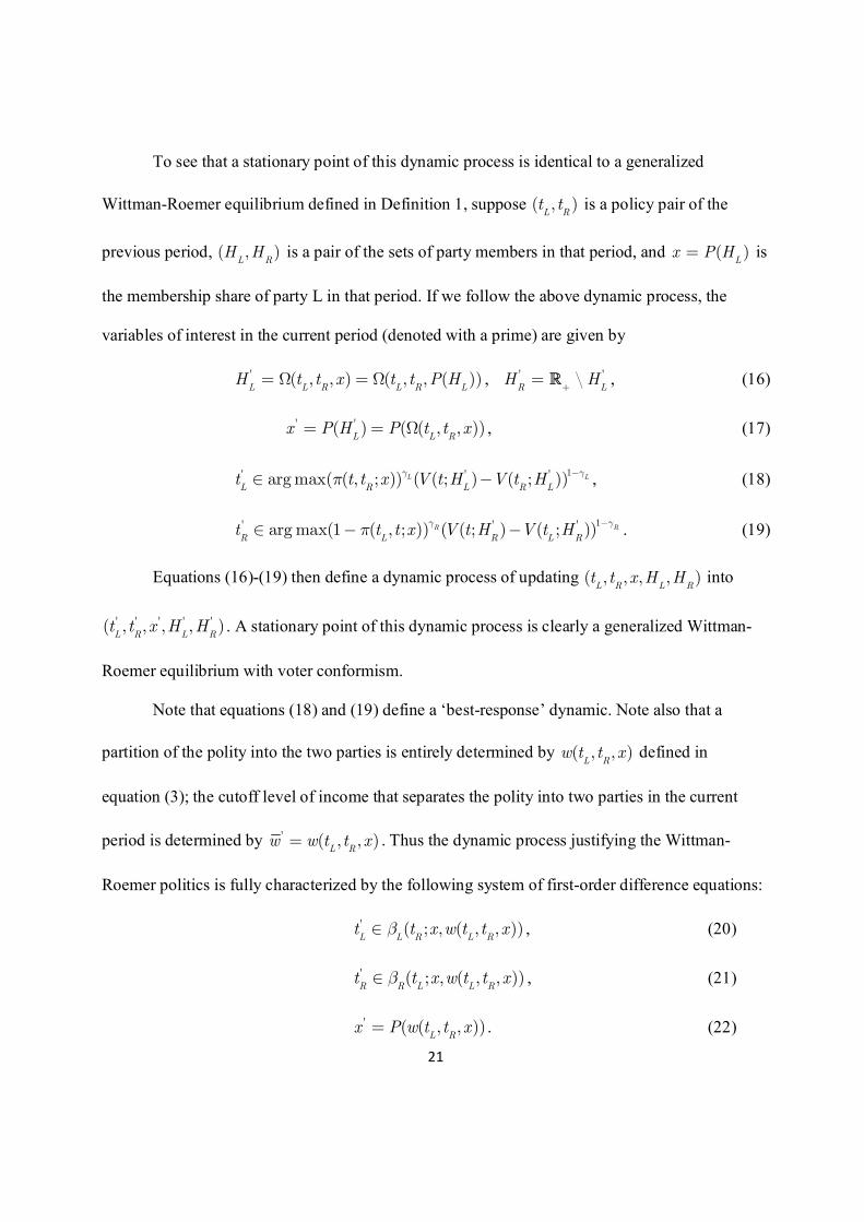
Equations (16)-(19) then define a dynamic process of updating ( , , , , )L R L Rt t x H H into
' ' ' ' '( , , , , )L R L Rt t x H H . A stationary point of this dynamic process is clearly a generalized Wittman-
Roemer equilibrium with voter conformism.
Note that equations (18) and (19) define a ‘best-response’ dynamic. Note also that a
partition of the polity into the two parties is entirely determined by ( , , )L R
w t t x defined in
equation (3); the cutoff level of income that separates the polity into two parties in the current
period is determined by ' ( , , )L R
w w t t x= . Thus the dynamic process justifying the Wittman-
Roemer politics is fully characterized by the following system of first-order difference equations:
' ( ; , ( , , ))L L R L Rt t x w t t xbÎ , (20)
' ( ; , ( , , ))R R L L Rt t x w t t xbÎ , (21)
' ( ( , , ))L R
x P w t t x= . (22)
22
Best responses are well defined for all , [0,1)L R
g g Î , and so is the best-response dynamic.
As we discussed earlier in this section, ( , , )R
t t xp is discontinuous at R
t t= if 12
( ) 0xq - = , and
continuous everywhere if 12
( ) 0xq - ¹ . (See Figure 1 again.) This implies that best responses
may not be well defined if 1L
g = and 12
( ) 0xq - = . If 1L
g ¹ , on the other hand,
1( ( , , )) ( ( ; ) ( ; ))L L
R L R Lt t x V t H V t H
g gp
-- is always continuous in t , even in the case of
12
( ) 0xq - = . This is because as R
t t® , ( ; ) ( ; ) 0L R L
V t H V t H- ® while ( , , )R
t t xp approaches
to a finite number. Thus it is only the Hotelling-Downs parties that may not have a best response
to some of its opponent’s policies.
There may exist multiple best responses. In that case, we will assume that parties choose
the ones close to what they chose in the previous period. This assumption is particularly important
when there are multiple equilibria. 10
Finally, we briefly remark that there may exist ‘trivial’ non-differentiated equilibria in the
generalized Wittman-Roemer model of political competition. If (.)F is ‘symmetric,’ for instance,
* * 12
( , , )t t , where *t is the ideal tax rate of the voter with the median (mean) income, is an
equilibrium for all , [0,1]L R
g g Î .11 Other trivial non-differentiated equilibria may also exist, if we
further specify the functional forms of (.)h and (.)f . These equilibria are not of our interest. (In
10 We argue only that the above-mentioned best-response dynamic justifies the generalized Wittman-Roemer
equilibrium with voter conformism, not that the best-response dynamic that we use in the paper is the only
‘reasonable’ dynamic for justifying it. Which dynamic is more reasonable is not our concern.
11 Here is a sketch of the proof. If both parties propose an identical policy at the expected membership share of ½, the
actual membership share is also ½. At the membership share of ½, no party would like to deviate unilaterally if the
income distribution is symmetric because the policy is optimal for both the militants and the opportunists when the
other party is holding that policy.
23
any way, no real income distribution is symmetric.) They are not generic; we are more interested
in ‘generic’ equilibria.
3. The Hotelling-Downs model of political competition when voter conformism is present
We first study the political equilibrium of the Hotelling-Downs model when voter
conformism is present. This is the case of 1L R
g g= = in our formulation.
In the original Hotelling-Downs model without voter conformism, a pair of Condorcet
winners constitutes a political equilibrium. In the model with voter conformism, which policy will
be a Condorcet winner depends, in general, upon the expected membership share x . We define a
strict x -Condorcet winner to be a policy that defeats all other policies in pairwise elections at the
expected membership share of x .
We now prove:
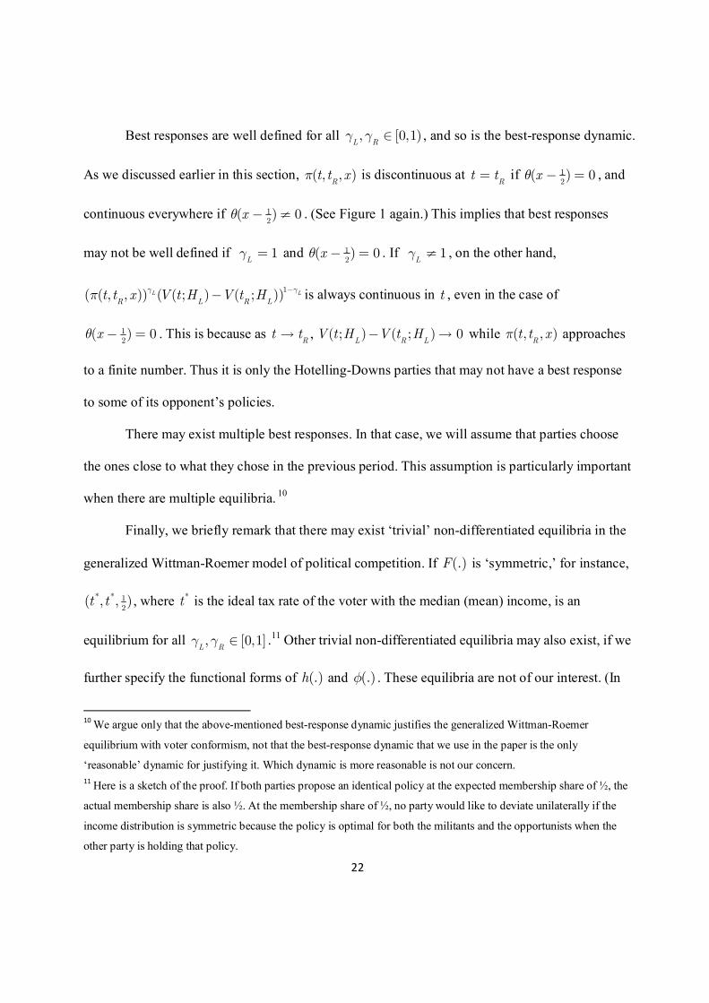
Theorem 1: The unique Hotelling-Downs equilibrium with voter conformism is
* * * * * 12
( , , ) ( , , )L Rt t x t t= , where *t is a strict 1
2-Condorcet winner. The equilibrium party
membership is an arbitrary random half subset of +
R for each party.
Thus were real politics a Hotelling-Downs kind, there would be no differentiation of
policies between political parties, and voter conformism would have no consequence on party
platforms or policies; parties would propose the same policy whatever the types of voter
conformism. Note that the theorem does not require any assumption on (.)F .
24
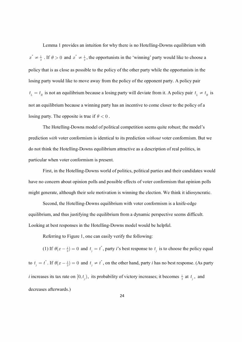
Lemma 1 provides an intuition for why there is no Hotelling-Downs equilibrium with
* 12
x ¹ . If 0q > and * 12
x ¹ , the opportunists in the ‘winning’ party would like to choose a
policy that is as close as possible to the policy of the other party while the opportunists in the
losing party would like to move away from the policy of the opponent party. A policy pair
L Rt t= is not an equilibrium because a losing party will deviate from it. A policy pair
L Rt t¹ is
not an equilibrium because a winning party has an incentive to come closer to the policy of a
losing party. The opposite is true if 0q < .
The Hotelling-Downs model of political competition seems quite robust; the model’s
prediction with voter conformism is identical to its prediction without voter conformism. But we
do not think the Hotelling-Downs equilibrium attractive as a description of real politics, in
particular when voter conformism is present.
First, in the Hotelling-Downs world of politics, political parties and their candidates would
have no concern about opinion polls and possible effects of voter conformism that opinion polls
might generate, although their sole motivation is winning the election. We think it idiosyncratic.
Second, the Hotelling-Downs equilibrium with voter conformism is a knife-edge
equilibrium, and thus justifying the equilibrium from a dynamic perspective seems difficult.
Looking at best responses in the Hotelling-Downs model would be helpful.
Referring to Figure 1, one can easily verify the following:
(1) If 12
( ) 0xq - = and *
jt t= , party i’s best response to
jt is to choose the policy equal
to *
jt t= . If 1
2( ) 0xq - = and *
jt t¹ , on the other hand, party i has no best response. (As party
i increases its tax rate on [0, )jt , its probability of victory increases; it becomes 1
2 at
jt , and
decreases afterwards.)
25
(2) If 12
( ) 0xq - > , party i has a continuum of best responses, which always includes jt .
(If 12
( ) 0xq - > , party i can have ‘all’ voters as its party members by choosing the same policy
as the opponent’s.) In this case, party i may use a random device to choose one among many.
(3) If 12
( ) 0xq - < , party i has a best response that is not equal to jt . (Choosing
jt is the
worst option for party i in this case, because the entire polity will turn away from the party.)
Thus unless the initial expected fraction of voters who prefer L to R is precisely equal to
12
, and the initial pair of policies is exactly that of strict 12
-Condorcet winners, the dynamic
process may stuck in the middle (due to the absence of a best response), or simply drift away from
the equilibrium (due to the multiplicity of best responses). We conjecture, without a proof, that
the probability that the dynamic process the Hotelling-Downs politics converges to the
equilibrium is zero.
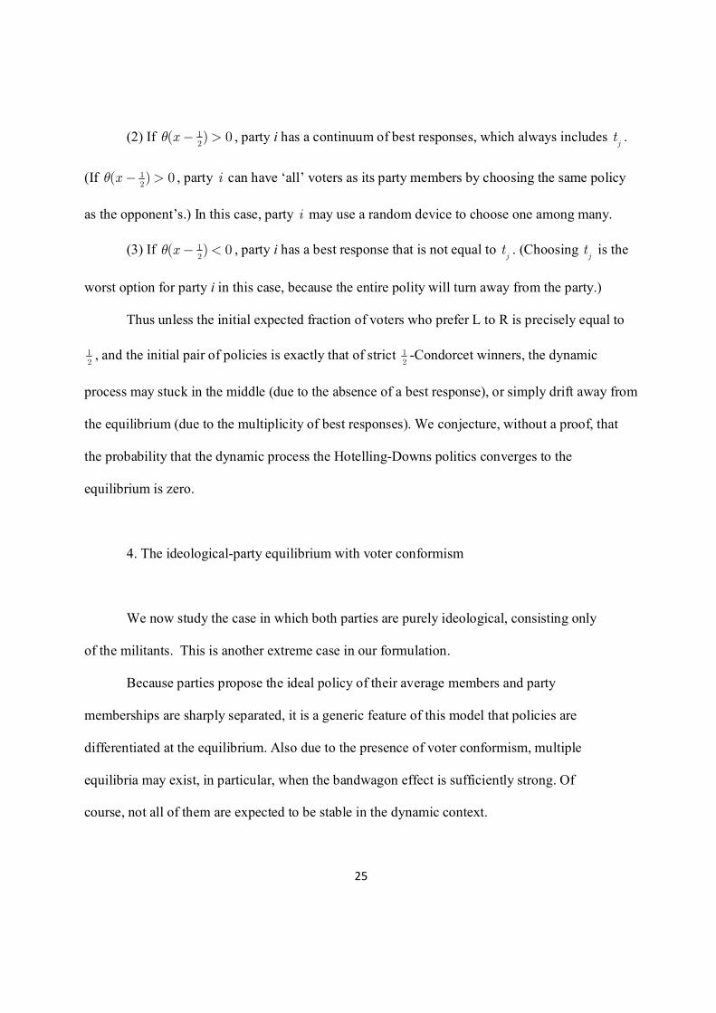
4. The ideological-party equilibrium with voter conformism
We now study the case in which both parties are purely ideological, consisting only
of the militants. This is another extreme case in our formulation.
Because parties propose the ideal policy of their average members and party
memberships are sharply separated, it is a generic feature of this model that policies are
differentiated at the equilibrium. Also due to the presence of voter conformism, multiple
equilibria may exist, in particular, when the bandwagon effect is sufficiently strong. Of
course, not all of them are expected to be stable in the dynamic context.
26
As we remarked earlier, this model would be trivial without endogenous party
membership or voter conformism. To be precise, the model is not game-theoretic; each party
simply chooses the ideal policy of its average member. The model is, however, nontrivial
when party membership is endogenously determined and voter conformism is present. Our
study in this section will also shed some lights on the classical Wittman-Roemer model of
political competition that will be studied in section 5.
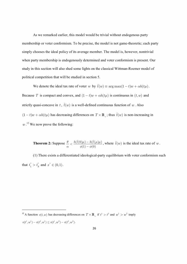
We denote the ideal tax rate of voter w by ( ) arg max(1 ) ( )t w t w h ta mº - +% .
Because T is compact and convex, and (1 ) ( )t w h ta m- + is continuous in ( , )t w and
strictly quasi-concave in t , ( )t w% is a well-defined continuous function of w . Also
(1 ) ( )t w h ta m- + has decreasing differences on T+
´R ; thus ( )t w% is non-increasing in
w .12 We now prove the following:
Theorem 2: Suppose ( (0) ) ( ( ) )
(1) (0)
h t h tq m m m
a f f
-<
-
% %, where ( )t w% is the ideal tax rate of w .
(1) There exists a differentiated ideological-party equilibrium with voter conformism such
that * *
L Rt t> and * (0,1)x Î .
12
A function ( , )v t w has decreasing differences on T+
´R if 1 2t t> and 1 2w w> imply
1 1 2 1 1 2 2 2( , ) ( , ) ( , ) ( , )v t w v t w v t w v t w- £ - .
27
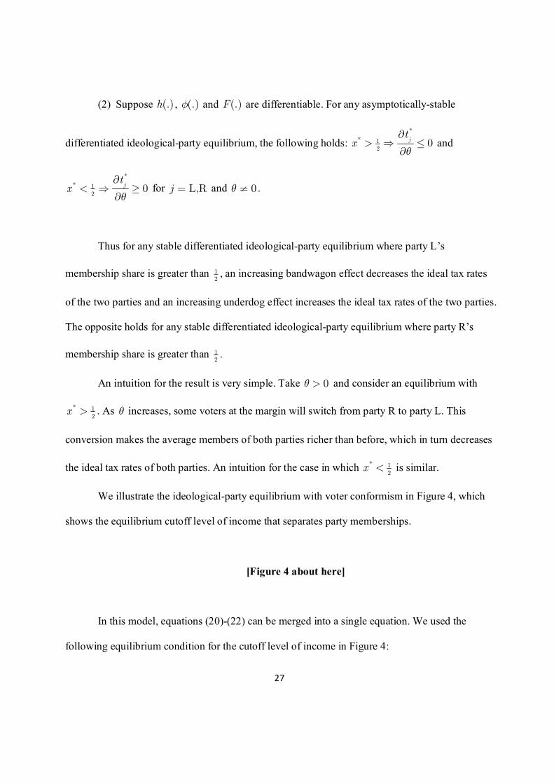
(2) Suppose (.)h , (.)f and (.)F are differentiable. For any asymptotically-stable
differentiated ideological-party equilibrium, the following holds:
*
* 12
0jt
xq
¶> Þ £
¶ and
*
* 12
0jt
xq
¶< Þ ³
¶ for L,Rj = and 0q ¹ .
Thus for any stable differentiated ideological-party equilibrium where party L’s
membership share is greater than 12
, an increasing bandwagon effect decreases the ideal tax rates
of the two parties and an increasing underdog effect increases the ideal tax rates of the two parties.
The opposite holds for any stable differentiated ideological-party equilibrium where party R’s
membership share is greater than 12
.
An intuition for the result is very simple. Take 0q > and consider an equilibrium with
* 12
x > . As q increases, some voters at the margin will switch from party R to party L. This
conversion makes the average members of both parties richer than before, which in turn decreases
the ideal tax rates of both parties. An intuition for the case in which * 12
x < is similar.
We illustrate the ideological-party equilibrium with voter conformism in Figure 4, which
shows the equilibrium cutoff level of income that separates party memberships.
[Figure 4 about here]
In this model, equations (20)-(22) can be merged into a single equation. We used the
following equilibrium condition for the cutoff level of income in Figure 4:
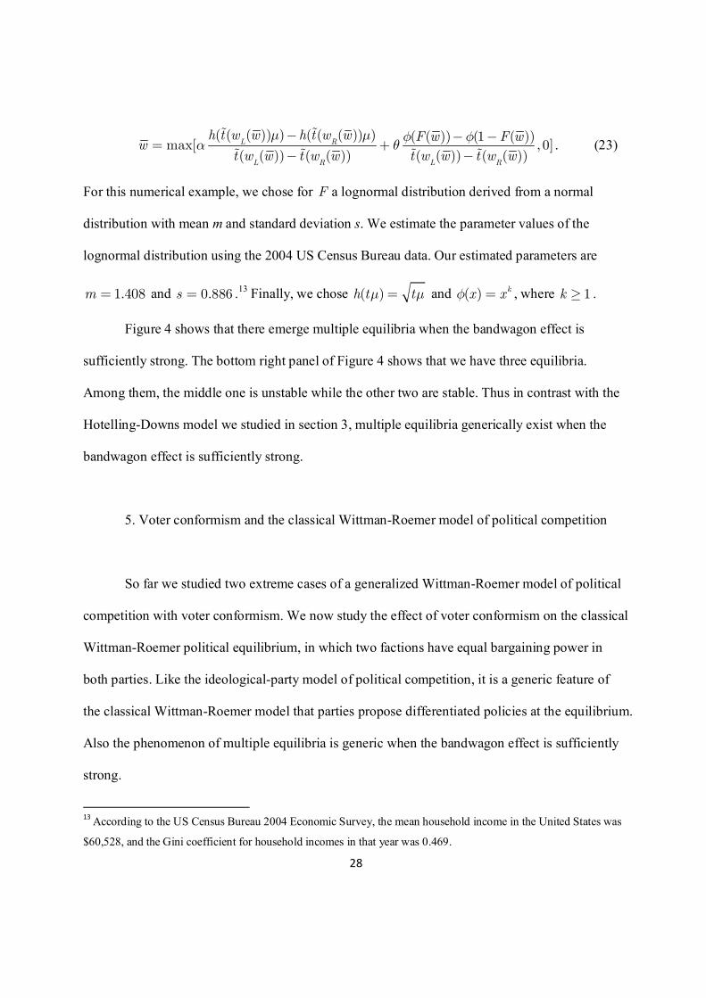
28
( ( ( )) ) ( ( ( )) ) ( ( )) (1 ( ))max[ , 0]
( ( )) ( ( )) ( ( )) ( ( ))L R
L R L R
h t w w h t w w F w F ww
t w w t w w t w w t w w
m m f fa q
- - -= +
- -
% %
% % % %. (23)
For this numerical example, we chose for F a lognormal distribution derived from a normal
distribution with mean m and standard deviation s. We estimate the parameter values of the
lognormal distribution using the 2004 US Census Bureau data. Our estimated parameters are
1.408m = and 0.886s = .13 Finally, we chose ( )h t tm m= and ( ) kx xf = , where 1k ³ .
Figure 4 shows that there emerge multiple equilibria when the bandwagon effect is
sufficiently strong. The bottom right panel of Figure 4 shows that we have three equilibria.
Among them, the middle one is unstable while the other two are stable. Thus in contrast with the
Hotelling-Downs model we studied in section 3, multiple equilibria generically exist when the
bandwagon effect is sufficiently strong.
5. Voter conformism and the classical Wittman-Roemer model of political competition
So far we studied two extreme cases of a generalized Wittman-Roemer model of political
competition with voter conformism. We now study the effect of voter conformism on the classical
Wittman-Roemer political equilibrium, in which two factions have equal bargaining power in
both parties. Like the ideological-party model of political competition, it is a generic feature of
the classical Wittman-Roemer model that parties propose differentiated policies at the equilibrium.
Also the phenomenon of multiple equilibria is generic when the bandwagon effect is sufficiently
strong.
13
According to the US Census Bureau 2004 Economic Survey, the mean household income in the United States was
$60,528, and the Gini coefficient for household incomes in that year was 0.469.
29
A general characterization of the classical Wittman-Roemer equilibrium with voter
conformism is somewhat difficult to obtain. Thus we will calculate them numerically. In the
numerical computation, we chose the same functions used in section 4. For (.)F , we set
( ) ( 0.5)x G xF = - , where (.)G is a normal distribution with mean 0 and standard deviation 0.05.
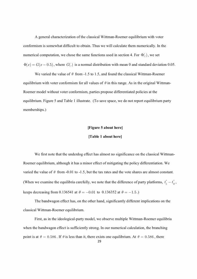
We varied the value of q from -1.5 to 1.5, and found the classical Wittman-Roemer
equilibrium with voter conformism for all values of q in this range. As in the original Wittman-
Roemer model without voter conformism, parties propose differentiated policies at the
equilibrium. Figure 5 and Table 1 illustrate. (To save space, we do not report equilibrium party
memberships.)
[Figure 5 about here]
[Table 1 about here]
We first note that the underdog effect has almost no significance on the classical Wittman-
Roemer equilibrium, although it has a minor effect of mitigating the policy differentiation. We
varied the value of q from -0.01 to -1.5, but the tax rates and the vote shares are almost constant.
(When we examine the equilibria carefully, we note that the difference of party platforms, * *
L Rt t- ,
keeps decreasing from 0.136541 at 0.01q =- to 0.136352 at 1.5q =- .)
The bandwagon effect has, on the other hand, significantly different implications on the
classical Wittman-Roemer equilibrium.
First, as in the ideological-party model, we observe multiple Wittman-Roemer equilibria
when the bandwagon effect is sufficiently strong. In our numerical calculation, the branching
point is at 0.586q = . If q is less than it, there exists one equilibrium. At 0.586q = , there
30
emerge two equilibria. After that, one of the two equilibria branches into two separate equilibria.
Thus, if 0.586q > , there always exist three equilibria. When multiple equilibria exist, we call
them type-A, type-B, and type-C equilibria. A type-A equilibrium is the one in which *x is
significantly less than 0.5, a type-B equilibrium is that in which *x is significantly greater than
0.5, and a type-C equilibrium is the one in which *x is between them, which is nearby 0.5. We
plot the three types of equilibria separately in Figure 5.
It is not easy to merge equations (20)-(22) into one in this model. We thus checked the
stability of Wittman-Roemer equilibria by calculating the Jacobian of the system of equations
(20)-(22). If eigenvalues of the Jacobian are all less than 1 in their absolute terms, it would be
asymptotically stable in a dynamic context. We find that all type-A and type-B equilibria are
asymptotically stable while all type-C equilibria are not. Thus more meaningful equilibria in a
dynamic context are those of type-A and type-B.
In type-A and type B equilibria, political parties diverge more as the bandwagon effect
becomes larger.14 We thus observe that in dynamically stable classical Wittman-Roemer
equilibria, an increasing bandwagon effect exacerbates the policy differentiation of the two parties.
The classical Wittman-Roemer equilibrium is sharply in contrast with the ideological-
party equilibrium, where parties move in the same direction as the degree of voter conformism
changes; the classical Wittman-Roemer parties move in an opposite direction as the parameter
that captures the degree of voter conformism increases.
14 In type-C equilibria, on the other hand, the difference in policies between the two parties is almost constant. When
we examine the type-C equilibria carefully, we note that the difference of party platforms, * *
L Rt t- , keeps decreasing
from 0.1383 at 0.59q = to 0.13625 at 0.98q = , and afterwards increases up to 0.13626 at 1.5q = . But such
changes are almost unnoticeable.
31
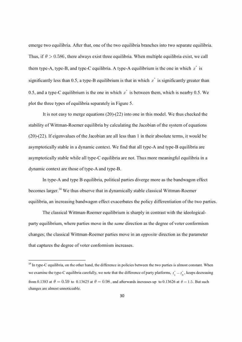
It would be useful to see how factions in each party bargain to an equilibrium policy,
taking the equilibrium policy of the opposition party as given. Recall that at a generalized
Wittman-Roemer equilibrium, neither party’s factions can unanimously agree to alter their
proposal. Any policy that increases both factions’ payoffs cannot be a Wittman-Roemer
equilibrium; given the policy played by the opposition party, if a move from *
it increases the
payoff of party i’s militants, then it must decrease the payoff of party i’s opportunists. Thus
the bargaining outcome lies always in the Pareto mini frontier defined by the payoff
functions of the two factions calculated at the opposition party’s policy.
We illustrate this point in Figure 6.
[Figure 6 about here]
We chose type-A and type-B equilibria at 0.9q = . In each figure, we draw the
payoff functions of the two factions, computed at the equilibrium policy of the opposition
party, and the equilibrium tax rate (vertical line).The two dots before and after the vertical
line represents the policies that determine the boundaries of the Pareto mini frontier. Any
policy outside the interval determined by the two dots will not be agreed upon within a party
because both factions can be better off by deviating from it to a policy inside the interval.
The precise location of the equilibrium policy inside the interval is determined by equation
(14) or (15).
We now provide an intuition behind the main results in this section. We will consider the
bandwagon effect only; the underdog effect can be explained in similar ways.
32
Suppose party R is winning ( * 12
x < ), as in a type-A equilibrium. Pick any level of 0q > .
At the current level of q , a proposal of R-militants to change the current R policy to the direction
of the ideal tax rate of its average member would not be agreed upon within the party because it
would require a sacrifice of R-opportunists. If the value of q increases, however, it gives a
windfall gain to R-opportunists, because more voters will lean toward R even at the same policy
pairs. Thus, without sacrificing its opportunists, party R can change its policy slightly to the
direction of the ideal tax rate of its average member.
The intuition for the direction of a policy change in the losing party, in this case party L, is
different from that for the winning party. According to Lemma 1 of section 2, the opportunists of
a ‘losing party’ can be better off by moving away from the policy of the opposition party. The
higher the value of q , the stronger the incentive of the opportunists of a losing party to move
away from the policy of the opponent. Such a move will be agreed upon by the militants of party
L, because it implies that the party policy will be closer to the ideal policy of the militants.
An explanation for the case in which party L is winning, as in the type-B equilibrium, is
similar. An increase in q in this situation gives a windfall gain to L-opportunists; thus L-militants
can call for a higher tax rate without scarifying L-opportunists. At the same time, party R’s
opportunists propose a policy which is further distant from the policy of party L.
The above explanations based on the Nash bargaining perspective also provide an
intuition for why neither bandwagon nor underdog has much impact on the policy differences
when the vote share is nearby 0.5. If the vote share is close to 0.5, windfall gains to the
opportunists of the winning party are very small; there is not much room for bargaining for policy
changes. Also the change that the opportunists of a losing party demand will be small.
33
6. Conclusion
Using the framework of the generalized Wittman-Roemer model of political competition,
we studied the potential effect that voter conformism might have on the political equilibrium of
various models. The current paper shows that the effect of voter conformism on the nature of
political equilibrium is quite different depending on the model one uses.
We find that voter conformism, both bandwagon and underdog, has no effect on the
Hotelling-Downs political equilibrium. Even if voter conformism is present, the Hotelling-Downs
parties propose an identical policy at the equilibrium, which is equal to a strict ½ -Condorcet
winner. But such an equilibrium seems difficult to justify in a dynamic context.
In the ideological-party model, political parties propose differentiated policies at the
equilibrium and the presence of multiple equilibria is generic when the bandwagon effect is
sufficiently strong. In those equilibria that are dynamically stable and have the membership share
of party L greater than 0.5 (less than 0.5), an increasing bandwagon effect decreases (increases)
the equilibrium tax rates of both parties; the opposite is true for the underdog effect
The Wittman-Roemer parties behave differently not only from the Hotelling-Downs
parties but also from the purely ideological ones. Unlike the Hotelling-Downs parties but like the
purely ideological parties, the Wittman-Roemer parties propose differentiated equilibrium
policies, and the extent of such policy differentiation depends on voter conformism. Existence of
multiple equilibria for a sufficiently strong bandwagon effect is also generic. In contrast with the
purely ideological parties which move in the same direction as the degree of voter conformism
changes, the Wittman-Roemer parties move in an opposite direction as the parameter that captures
the degree of voter conformism increases. In those equilibria that are dynamically stable, the
34
stronger the bandwagon effect is, the more differentiated policies are. The opposite holds when
the underdog effect is present; an increasing underdog effect mitigates the policy differentiation
of the two parties, although that effect is not large.
The present paper studies the effect of voter conformism on political equilibrium in a uni-
dimensional policy space. It is well known that both the Hotelling-Downs and Wittman-Roemer
models of political competition do not possess generic equilibria when the policy space is multi-
dimensional. There are models that possess generic equilibria in a multi-dimensional policy space,
such as the probabilistic voting model of Lindbeck and Weibull (1987), or the party unanimity
Nash equilibrium model of Roemer (1999, 2001). We leave the study of the effect of voter
conformism on these models for future research.
35
References
Akerlof, George. 1997. “Social distance and social decisions.” Econometrica 65 (5): 1005-
1027.
Aldrich, John. 1980. “A dynamic model of presidential nomination campaigns.” American
Political Science Review 74 (3): 651-669
Banerjee, Abjit. 1992. “A simple model of herd behavior.” Quarterly Journal of
Economics 107 (3): 797-817.
Baron, David. 1993. “Government formation and endogenous parties.” American Political
Science Review 87 (1): 34-47.
Bartels, Larry. 1985. “Expectations and preferences in presidential nominating
campaigns.” American Political Science Review 79 (3): 804-815.
Bartels, Larry. 1988. Presidential Primaries and the Dynamics of Public Choice.
Princeton, NJ: Princeton University Press.
Baumol, William. 1957. “Interactions between successive polling results and voting
intentions.” Public Opinion Quarterly 21 (2): 318-323.
Bernheim, B. 1994, “A theory of conformity.” Journal of Political Economy 102 (5): 841-
877.
Birkhchandani, B. D. Hirshleifer, and I. Welch. 1992, “A theory of fads, fashion, custom,
and cultural change as informational cascades.” Journal of Political Economy 100 (5): 992-1026.
Downs, Anthony. 1957. An Economic Theory of Democracy. New York, NY: Harper.
36
Irwin, Galen, and Joop J. M. Van Holsteyn. 2000. "Bandwagons, underdogs, the Titanic,
and the Red Cross. The influence of public opinion polls on voters." Communication presented at
the 18th Congress of the International Political Science Association, Québec, 1-5 August, 2000.
Leibenstein, Harvey. 1950. “Bandwagon, snob, and Veblen effects in the theory of
consumer demand.” Quarterly Journal of Economics 64 (2): 183-207.
Lindbeck, Assar, and Jurgen Weibull. 1987. “Balanced budget redistribution as the
outcome of political competition.” Public Choice 52 (3): 273-297.
Ortuno-Ortin, Ignacio. 1997. “A spatial model of political competition and proportional
representation.” Social Choice and Welfare 14 (3): 427-438.
Ortuno-Ortin, Ignacio, and John Roemer. 1998. “Endogenous party formation and the
effect of income distribution on policy.” Mimeo, University of Alicante.
Roemer, John. 1997. “Political economic equilibrium when parties represent constituents:
The uni-dimensional case.” Social Choice and Welfare 14 (4): 479-520.
Roemer, John. 2001. Political Competition: Theory and Applications. Cambridge, MA:
Harvard University Press.
Schelling, Thomas. 1978. Micromotives and Macrobehavior. New York, NY: Norton.
Simon, Herbert. 1954. “Bandwagon and underdog effects and the possibility of election
prediction.” Public Opinion Quarterly 18 (3): 245-253.
37
Appendix
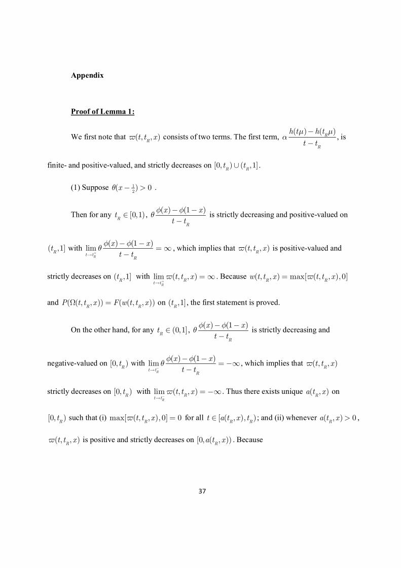
Proof of Lemma 1:
We first note that ( , , )R
t t xv consists of two terms. The first term, ( ) ( )
R
R
h t h t
t t
m ma
-
-, is
finite- and positive-valued, and strictly decreases on [0, ) ( ,1]R Rt tÈ .
(1) Suppose 12
( ) 0xq - > .
Then for any [0,1)Rt Î ,
( ) (1 )
R
x x
t t
f fq
- -
- is strictly decreasing and positive-valued on
( ,1]Rt with
( ) (1 )lim
Rt tR
x x
t t
f fq
+®
- -= ¥
-, which implies that ( , , )
Rt t xv is positive-valued and
strictly decreases on ( ,1]Rt with lim ( , , )
R
Rt t
t t xv+®
= ¥ . Because ( , , ) max[ ( , , ), 0]R R
w t t x t t xv=
and ( ( , , )) ( ( , , ))R R
P t t x F w t t xW = on ( ,1]Rt , the first statement is proved.
On the other hand, for any (0,1]Rt Î ,
( ) (1 )
R
x x
t t
f fq
- -
- is strictly decreasing and
negative-valued on [0, )Rt with
( ) (1 )lim
Rt tR
x x
t t
f fq
-®
- -=-¥
-, which implies that ( , , )
Rt t xv
strictly decreases on [0, )Rt with lim ( , , )
R
Rt t
t t xv-®
=-¥ . Thus there exists unique ( , )R
a t x on
[0, )Rt such that (i) max[ ( , , ), 0] 0
Rt t xv = for all [ ( , ), )
R Rt a t x tÎ ; and (ii) whenever ( , ) 0
Ra t x > ,
( , , )R
t t xv is positive and strictly decreases on [0, ( , ))R
a t x . Because
38
( ( , , )) 1 ( ( , , ))R R
P t t x F w t t xW = - on [0, )Rt and ( ( , , )) 1
R RP t t xW = , the second statement is
proved.
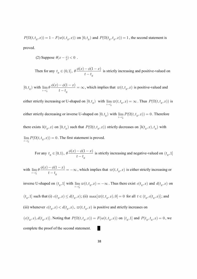
(2) Suppose 12
( ) 0xq - < .
Then for any (0,1]Rt Î ,
( ) (1 )
R
x x
t t
f fq
- -
- is strictly increasing and positive-valued on
[0, )Rt with
( ) (1 )lim
Rt tR
x x
t t
f fq
-®
- -= ¥
-, which implies that ( , , )
Rt t xv is positive-valued and
either strictly increasing or U-shaped on [0, )Rt with lim ( , , )
R
Rt t
t t xv-®
= ¥ . Thus ( ( , , ))R
P t t xW is
either strictly decreasing or inverse U-shaped on [0, )Rt with lim ( ( , , )) 0
R
Rt t
P t t x-®
W = . Therefore
there exists ( , )R
b t x on [0, )Rt such that ( ( , , ))
RP t t xW strictly decreases on [ ( , ), )
R Rb t x t with
lim ( ( , , )) 0R
Rt t
P t t x-®
W = . The first statement is proved.
For any [0,1)Rt Î ,
( ) (1 )
R
x x
t t
f fq
- -
- is strictly increasing and negative-valued on ( ,1]
Rt
with ( ) (1 )
limRt t
R
x x
t t
f fq
+®
- -=-¥
-, which implies that ( , , )
Rt t xv is either strictly increasing or
inverse U-shaped on ( ,1]Rt with lim ( , , )
R
Rt t
t t xv+®
=-¥ . Thus there exist ( , )R
c t x and ( , )R
d t x on
( ,1]Rt such that (i) ( , ) ( , )
R Rc t x d t x£ ; (ii) max[ ( , , ), 0] 0
Rt t xv = for all ( , ( , )]
R Rt t c t xÎ ; and
(iii) whenever ( , ) ( , )R R
c t x d t x< , ( , , )R
t t xv is positive and strictly increases on
( ( , ), ( , )]R R
c t x d t x . Noting that ( ( , , )) ( ( , , ))R R
P t t x F w t t xW = on ( ,1]Rt and ( , , ) 0
R RP t t x = , we
complete the proof of the second statement. █
39
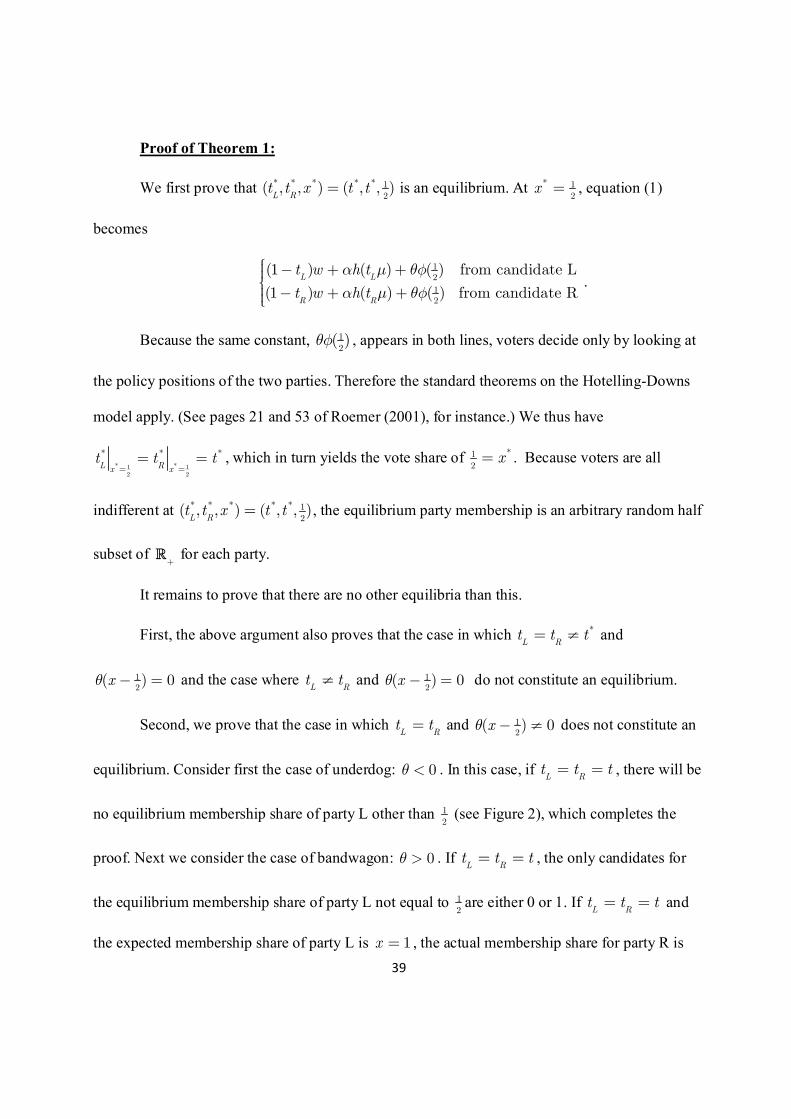
Proof of Theorem 1:
We first prove that * * * * * 1
2( , , ) ( , , )L Rt t x t t= is an equilibrium. At * 1
2x = , equation (1)
becomes
12
12
(1 ) ( ) ( ) from candidate L
(1 ) ( ) ( ) from candidate RL L
R R
t w h t
t w h t
a m qf
a m qf
ìï - + +ïíï - + +ïî
.
Because the same constant, 1
2( )qf , appears in both lines, voters decide only by looking at
the policy positions of the two parties. Therefore the standard theorems on the Hotelling-Downs
model apply. (See pages 21 and 53 of Roemer (2001), for instance.) We thus have
* *1 12 2
* * *
L Rx xt t t
= == = , which in turn yields the vote share of *1
2x= . Because voters are all
indifferent at * * * * * 1
2( , , ) ( , , )L Rt t x t t= , the equilibrium party membership is an arbitrary random half
subset of +
R for each party.
It remains to prove that there are no other equilibria than this.
First, the above argument also proves that the case in which *
L Rt t t= ¹
and
12
( ) 0xq - = and the case where L Rt t¹
and 1
2( ) 0xq - = do not constitute an equilibrium.
Second, we prove that the case in which L Rt t=
and 1
2( ) 0xq - ¹ does not constitute an
equilibrium. Consider first the case of underdog: 0q < . In this case, if L Rt t t= = , there will be
no equilibrium membership share of party L other than 1
2 (see Figure 2), which completes the
proof. Next we consider the case of bandwagon: 0q > . If L Rt t t= = , the only candidates for
the equilibrium membership share of party L not equal to 1
2are either 0 or 1. If
L Rt t t= = and
the expected membership share of party L is 1x = , the actual membership share for party R is
40
1 ( ( , ,1)) 0P t t- W = ; party R has an incentive to deviate. (By assumption 2, there is a profitable
direction of deviation.) If L Rt t t= = and the expected membership share of party L is 0x = , its
actual membership share is also 0; party L has an incentive to deviate.
Finally, we prove that any case in which L Rt t¹ and 1
2( ) 0xq - ¹
cannot be an
equilibrium. Suppose the actual membership share for party L at the triple is ( ( , , ))L R
P t t xW .
There are three cases.
Case 1: Suppose ( ( , , )) (0,1)L R
P t t xW Î at the triple. This means that party R’s
membership share at the triple is 1 ( ( , , )) (0,1)L R
P t t x- W Î . If 12
( ) 0xq - < , party R can
increases its actual membership share to 1 by choosing the policy that party L chooses. If
12
( ) 0xq - > , party L has an incentive to choose the same policy as party R’s.
Case 2: Suppose ( ( , , )) 0L R
P t t xW = at the triple. For all values of q and x , party L has
an incentive to deviate to a policy that gives it a positive membership share.
Case 3: Suppose ( ( , , )) 1L R
P t t xW = at the triple. For all values of q and x , party R has
an incentive to deviate to a policy that gives a positive membership share. █
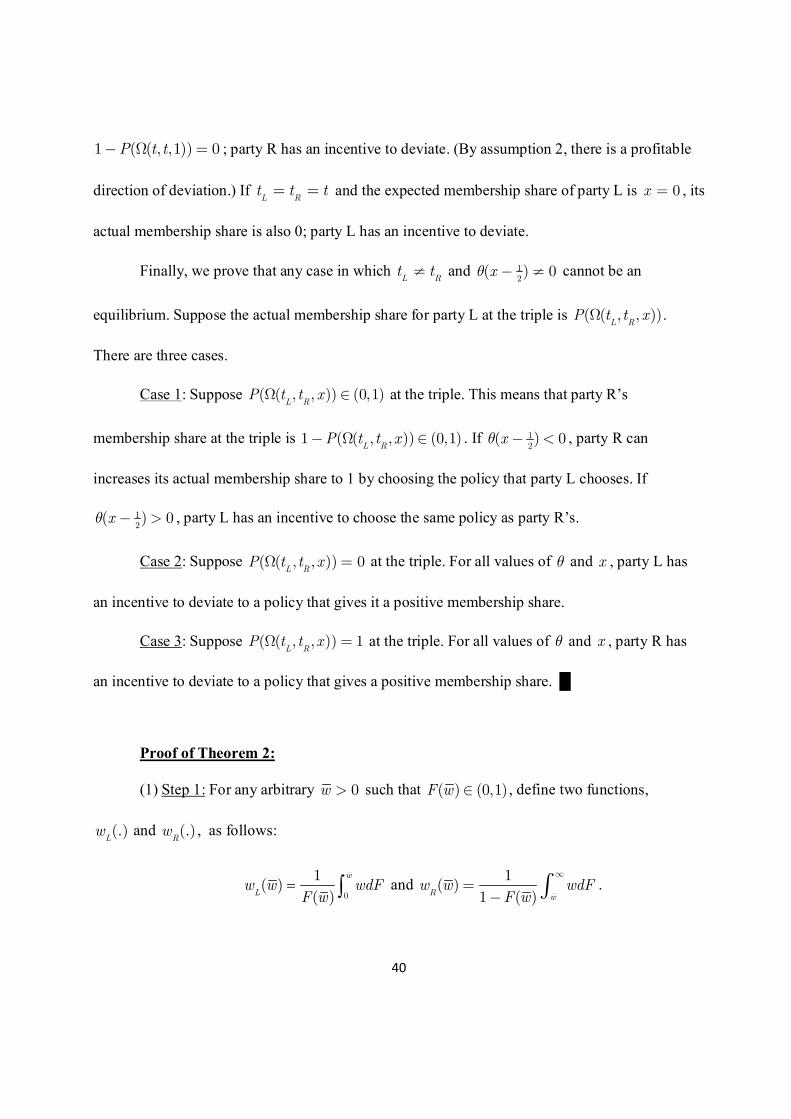
Proof of Theorem 2:
(1) Step 1: For any arbitrary 0w > such that ( ) (0,1)F w Î , define two functions,
(.)Lw and (.)
Rw , as follows:
0
1( )
( )
w
Lw w wdF
F w= ò and
1( )
1 ( )R ww w wdF
F w
¥
=- ò .
41
Note that (.)Lw and (.)
Rw are increasing continuous functions of w . Also note that
( ) ( )L Rw w w w< for all w . (Recall that F is strictly increasing.)
Step 2: We now show that there is a positive-valued fixed point of the map:
( ( ( )) ) ( ( ( )) ) ( ( )) (1 ( ))( )
( ( )) ( ( )) ( ( )) ( ( ))L R
L R L R
h t w w h t w w F w F ww
t w w t w w t w w t w w
m m f fv a q
- - -º +
- -
% %
% % % %.
The map (.)v is continuous: for ( ( )) ( ( ))L R
t w w t w w>% % , (.)h is strictly concave on T, and ( (.))j
t w%
is continuous. Thus, if (0) 0v > and ( )v ¥ <¥ , the map has a positive-valued fixed point. The
condition that ( )v ¥ <¥ holds because (.)f is finite-valued and (.)h is strictly concave. The
condition that (0) 0v > is ensured under the stated assumption.
Step 3: Denote the positive-valued fixed point by *w and define: * *[0, ]L
H w= ;
* *( , )R
H w= ¥ ; * *( ( ))j jt t w w= % , L,Rj = ; and * *( )x F w= . Then they clearly constitute an
ideological-party equilibrium with * *
L Rt t> and * (0,1)x Î .
(2) The full dynamic system in this model consists of four equations: ( ( ))j jt t w w= % ,
L,Rj = ; ( )x F w= ; and ' ( ) ( ) ( ) (1 )L R
L R L R
h t h t x xw
t t t t
m m f fa q
- - -= +
- -. Because it can be
reduced to a single difference equation, ' ( )w wv= , and the other three equations are not
difference equations, the condition for the stability of the dynamic system is: *( )
1w
w
v¶<
¶.
Fix q , and let *( )w q be the cutoff level of income evaluated at a dynamically stable
ideological-party equilibrium. Then we must have: * *( ) ( ( ))w wq v q= . Differentiating both sides,
42
we obtain:
( )
* * *
** *
( ) (1 )
( )1
L R
w x x
wt t
w
f f
q v
¶ - -=
æ ö¶ ¶ ÷ç ÷- -ç ÷ç ÷ç ¶è ø
. The denominator is positive if the equilibrium is
stable. The numerator is positive if * 12
x > and negative if * 12
x < . Thus *
* 12
0 0w
xq
¶- > Þ >
and *
* 12
0 0w
xq
¶- < Þ <
¶. The proof is complete by noting that *
jt is a non-increasing function
of *w . █
43
Figure 1: Actual membership shares
( ( , , ))L R
P t t xW 1 ( ( , , ))L R
P t t x- W
12
( ) 0xq - >
0.2 0.4 0.6 0.8 1.0tL
0.2
0.4
0.6
0.8
1.0
PHWHtL,tR,xLL
0.2 0.4 0.6 0.8 1.0tR
0.2
0.4
0.6
0.8
1.0
1-PHWHtL,tR,xLL
12
( ) 0xq - =
0.2 0.4 0.6 0.8 1.0tL
0.2
0.4
0.6
0.8
1.0
PHWHtL,tR,xLL
0.2 0.4 0.6 0.8 1.0tR
0.2
0.4
0.6
0.8
1.0
1-PHWHtL,tR,xLL
12
( ) 0xq - <
0.2 0.4 0.6 0.8 1.0tL
0.2
0.4
0.6
0.8
1.0
PHWHtL,tR,xLL
0.2 0.4 0.6 0.8 1.0tR
0.2
0.4
0.6
0.8
1.0
1-PHWHtL,tR,xLL
Note: Dots represent the place where the policy of the opposition party is held. These figures are
drawn while holding constant the policy of the opposition party and the expected membership
share of party L.
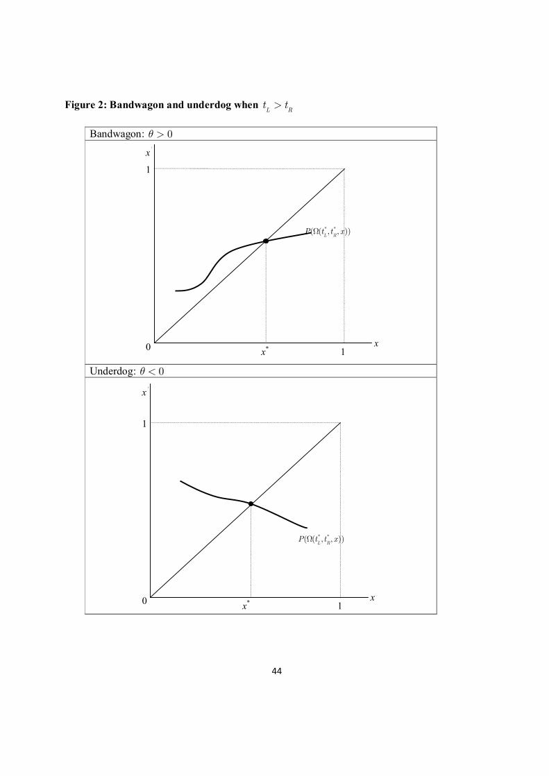
44
Figure 2: Bandwagon and underdog when L Rt t>
Bandwagon: 0q >
Underdog: 0q <
* *( ( , , ))L R
P t t xW
x
1
x*
x’
1 0
* *( ( , , ))L R
P t t xW
x
1
x*
x’
1 0
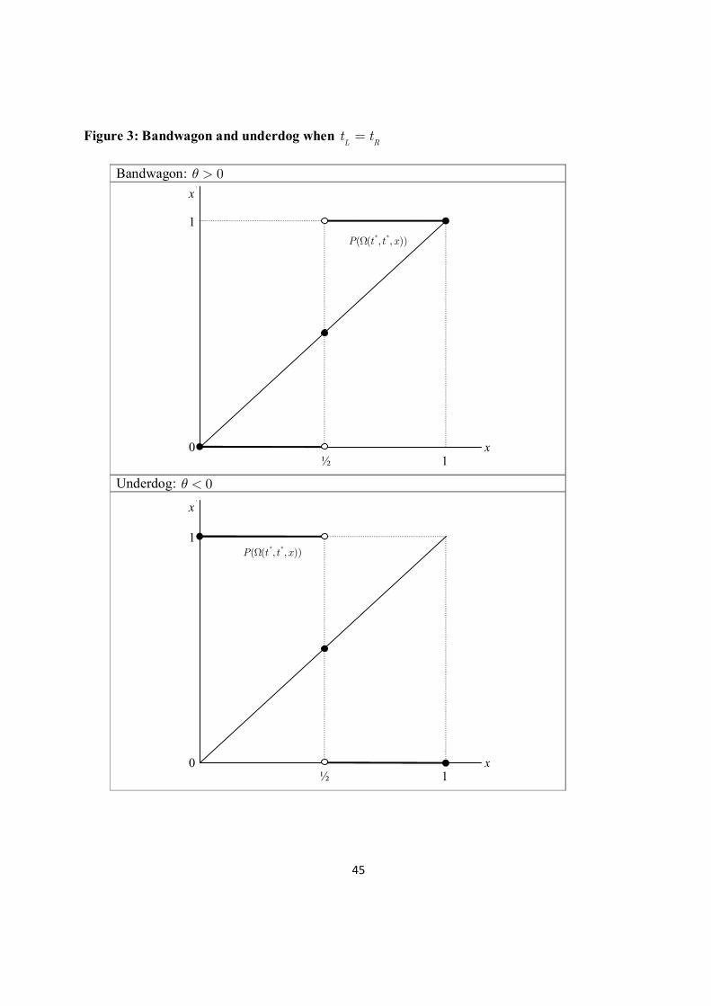
45
Figure 3: Bandwagon and underdog when L Rt t=
Bandwagon: 0q >
Underdog: 0q <
* *( ( , , ))P t t xW
x
1
x’
1 ½0
* *( ( , , ))P t t xW
x
1
x’
1 ½0
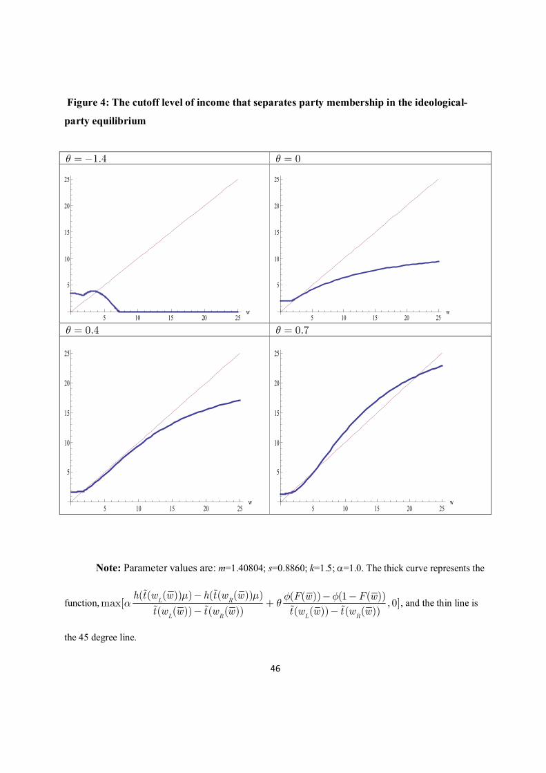
46
Figure 4: The cutoff level of income that separates party membership in the ideological-
party equilibrium
1.4q =- 0q =
5 10 15 20 25w
5
10
15
20
25
5 10 15 20 25w
5
10
15
20
25
0.4q = 0.7q =
5 10 15 20 25w
5
10
15
20
25
5 10 15 20 25w
5
10
15
20
25
Note: Parameter values are: m=1.40804; s=0.8860; k=1.5; a=1.0. The thick curve represents the
function,( ( ( )) ) ( ( ( )) ) ( ( )) (1 ( ))
max[ , 0]( ( )) ( ( )) ( ( )) ( ( ))L R
L R L R
h t w w h t w w F w F w
t w w t w w t w w t w w
m m f fa q
- - -+
- -
% %
% % % %, and the thin line is
the 45 degree line.
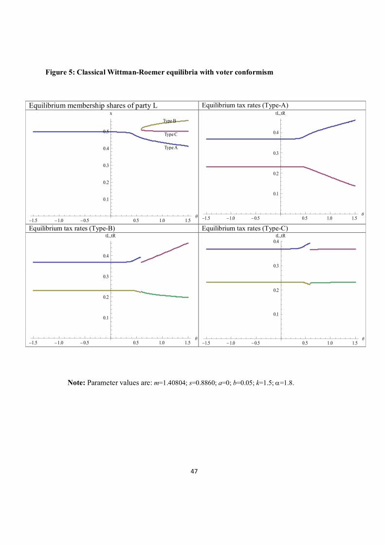
47
Figure 5: Classical Wittman-Roemer equilibria with voter conformism
Equilibrium membership shares of party L Equilibrium tax rates (Type-A)
Type B
Type C
Type A
-1.5 -1.0 -0.5 0.5 1.0 1.5q
0.1
0.2
0.3
0.4
0.5
x
-1.5 -1.0 -0.5 0.5 1.0 1.5q
0.1
0.2
0.3
0.4
tL,tR
Equilibrium tax rates (Type-B) Equilibrium tax rates (Type-C)
-1.5 -1.0 -0.5 0.5 1.0 1.5q
0.1
0.2
0.3
0.4
tL,tR
-1.5 -1.0 -0.5 0.5 1.0 1.5q
0.1
0.2
0.3
0.4tL,tR
Note: Parameter values are: m=1.40804; s=0.8860; a=0; b=0.05; k=1.5; a=1.8.
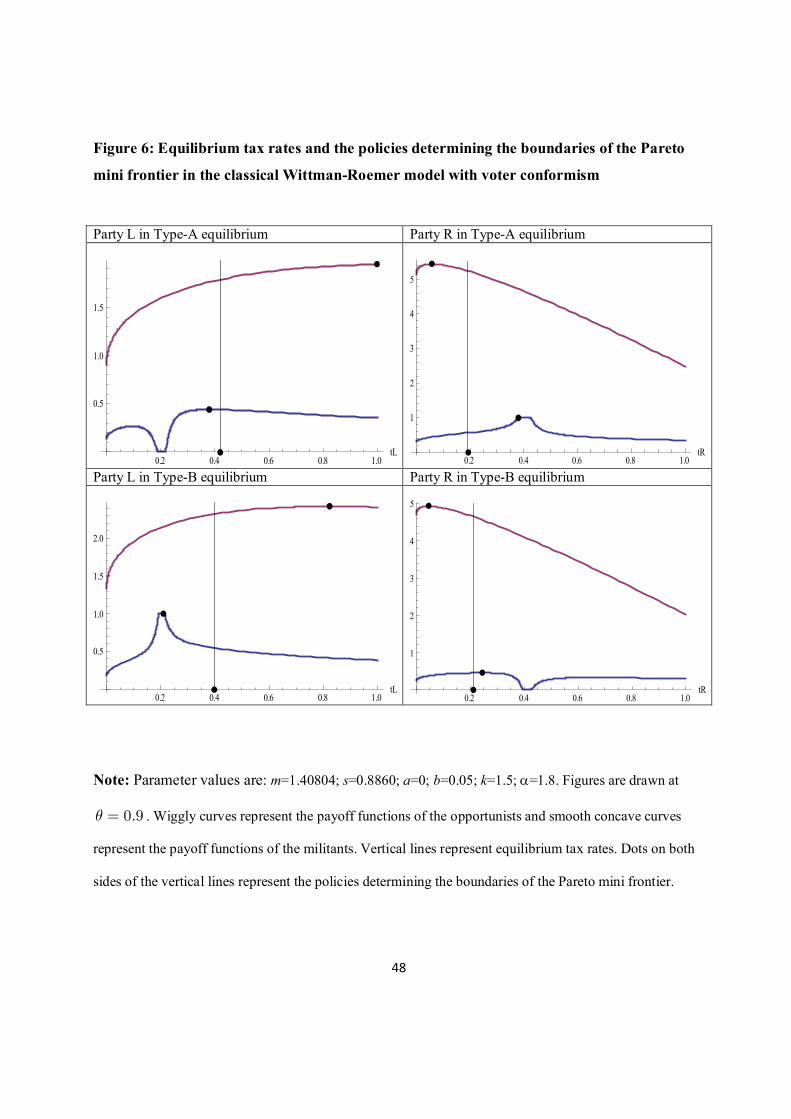
48
Figure 6: Equilibrium tax rates and the policies determining the boundaries of the Pareto
mini frontier in the classical Wittman-Roemer model with voter conformism
Party L in Type-A equilibrium Party R in Type-A equilibrium
0.2 0.4 0.6 0.8 1.0tL
0.5
1.0
1.5
0.2 0.4 0.6 0.8 1.0tR
1
2
3
4
5
Party L in Type-B equilibrium Party R in Type-B equilibrium
0.2 0.4 0.6 0.8 1.0tL
0.5
1.0
1.5
2.0
0.2 0.4 0.6 0.8 1.0tR
1
2
3
4
5
Note: Parameter values are: m=1.40804; s=0.8860; a=0; b=0.05; k=1.5; a=1.8. Figures are drawn at
0.9q = . Wiggly curves represent the payoff functions of the opportunists and smooth concave curves
represent the payoff functions of the militants. Vertical lines represent equilibrium tax rates. Dots on both
sides of the vertical lines represent the policies determining the boundaries of the Pareto mini frontier.
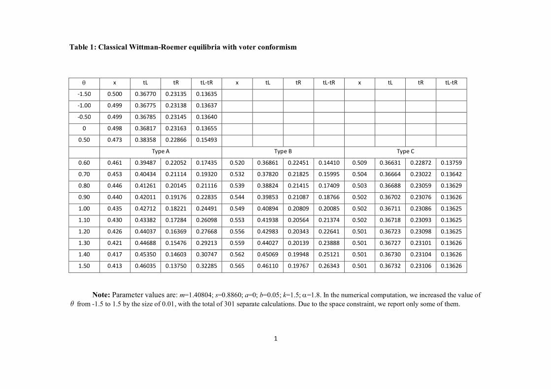
1
Table 1: Classical Wittman-Roemer equilibria with voter conformism
q x tL tR tL-tR x tL tR tL-tR x tL tR tL-tR
-1.50 0.500 0.36770 0.23135 0.13635
-1.00 0.499 0.36775 0.23138 0.13637
-0.50 0.499 0.36785 0.23145 0.13640
0 0.498 0.36817 0.23163 0.13655
0.50 0.473 0.38358 0.22866 0.15493
Type A Type B Type C
0.60 0.461 0.39487 0.22052 0.17435 0.520 0.36861 0.22451 0.14410 0.509 0.36631 0.22872 0.13759
0.70 0.453 0.40434 0.21114 0.19320 0.532 0.37820 0.21825 0.15995 0.504 0.36664 0.23022 0.13642
0.80 0.446 0.41261 0.20145 0.21116 0.539 0.38824 0.21415 0.17409 0.503 0.36688 0.23059 0.13629
0.90 0.440 0.42011 0.19176 0.22835 0.544 0.39853 0.21087 0.18766 0.502 0.36702 0.23076 0.13626
1.00 0.435 0.42712 0.18221 0.24491 0.549 0.40894 0.20809 0.20085 0.502 0.36711 0.23086 0.13625
1.10 0.430 0.43382 0.17284 0.26098 0.553 0.41938 0.20564 0.21374 0.502 0.36718 0.23093 0.13625
1.20 0.426 0.44037 0.16369 0.27668 0.556 0.42983 0.20343 0.22641 0.501 0.36723 0.23098 0.13625
1.30 0.421 0.44688 0.15476 0.29213 0.559 0.44027 0.20139 0.23888 0.501 0.36727 0.23101 0.13626
1.40 0.417 0.45350 0.14603 0.30747 0.562 0.45069 0.19948 0.25121 0.501 0.36730 0.23104 0.13626
1.50 0.413 0.46035 0.13750 0.32285 0.565 0.46110 0.19767 0.26343 0.501 0.36732 0.23106 0.13626
Note: Parameter values are: m=1.40804; s=0.8860; a=0; b=0.05; k=1.5; a=1.8. In the numerical computation, we increased the value of
q from -1.5 to 1.5 by the size of 0.01, with the total of 301 separate calculations. Due to the space constraint, we report only some of them.