DEPARTMENT OF ECONOMICS AND FINANCE

COLLEGE OF BUSINESS AND ECONOMICS

UNIVERSITY OF CANTERBURY

CHRISTCHURCH, NEW ZEALAND

Investor Preferences for Oil Spot and Futures

Based on Mean-Variance and Stochastic Dominance

Hooi Hooi Lean, Michael McAleer & Wing-Keung Wong

WORKING PAPER

No. 22/2010

Department of Economics and Finance College of Business and Economics

University of Canterbury Private Bag 4800, Christchurch

New Zealand

1

WORKING PAPER No. 22/2010

Investor Preferences for Oil Spot and Futures

Based on Mean-Variance and Stochastic Dominance

Hooi Hooi Lean1, Michael McAleer

2, and Wing-Keung Wong

3

May 2010

Abstract: This paper examines investor preferences for oil spot and futures based on

mean-variance (MV) and stochastic dominance (SD). The mean-variance criterion

cannot distinct the preferences of spot and market whereas SD tests leads to the

conclusion that spot dominates futures in the downside risk while futures dominate

spot in the upside profit. It is also found that risk-averse investors prefer investing in

the spot index, whereas risk seekers are attracted to the futures index to maximize

their expected utilities. In addition, the SD results suggest that there is no arbitrage

opportunity between these two markets. Market efficiency and market rationality are

likely to hold in the oil spot and futures markets.

Keywords: Stochastic dominance, risk averter, risk seeker, futures market, spot

market.

JEL Classifications: C14, G12, G15.

Acknowledgements: The first author would like to acknowledge Universiti Sains

Malaysia RU Grant No. 1001/PSOSIAL/816094. The second author wishes to

acknowledge the financial support of the Australian Research Council, National

Science Council, Taiwan, Center for International Research on the Japanese Economy

(CIRJE), Faculty of Economics, University of Tokyo, and a Visiting Erskine

Fellowship at the University of Canterbury, New Zealand. The third author would like

to thank Robert B. Miller and Howard E. Thompson for their continuous guidance

and encouragement, and to acknowledge the financial support of Hong Kong Baptist

University.

1Economics Program, School of Social Sciences, Universiti Sains Malaysia

2Econometric Institute, Erasmus School of Economics, Erasmus University of

Rotterdam and Tinbergen Institiute, The Netherlands, and Department of Economics

and Finance, University of Canterbury, New Zealand 3Department of Economics, Hong Kong Baptist University

Corresponding Author: Michael McAleer, email: michael.mcaleer@gmail.com

2

WORKING PAPER No. 22/2010

Investor Preferences for Oil Spot and Futures

Based on Mean-Variance and Stochastic Dominance

Introduction

Crude oil is an important commodity for the world economy. With the increasing

tension of crude oil price, oil futures have became a popular derivative to hedge

against the risk of possible oil price changes. Spot and futures prices of oil have been

investigated over an extended period. Substantial research has been undertaken to

analyze the relationship between spot and futures prices, and their associated returns.

The efficient market hypothesis is crucial for understanding optimal decision making

with regard to hedging and speculation, and also for making financial decisions about

the optimal allocation of portfolios of assets with regard to their multivariate returns

and associated risks.

The literature on the relationships between spot and futures prices of petroleum

products has examined issues such as market efficiency and price discovery. Bopp

and Sitzer (1987) find that futures prices have a significant positive contribution to

describe past price changes, even when crude oil prices, inventory levels, weather,

and other important variables are accounted for. Serletis and Banack (1990) use daily

data for the spot and two-month futures crude oil prices, and for prices of gasoline and

heating oil traded on the New York Stock Exchange (NYMEX), to test for market

efficiency. They find evidence in support of the market efficiency hypothesis.

Crowder and Hamid (1993) use cointegration analysis to test the simple efficiency

hypothesis and the arbitrage condition for crude oil futures. Their results support the

simple efficiency hypothesis that the expected returns from futures speculation in the

oil futures market are zero.

In the price discovery literature, Quan (1992) examines the price discovery

process for the crude oil market using monthly data, and finds that futures prices do

not play an important role in this process. Using daily data from NYMEX closing

3

futures prices, Schwartz and Szakmary (1994) find that futures prices strongly

dominate in the price discovery process relative to the deliverable spots in all three

petroleum markets. Gulen (1999) applies cointegration tests in a series of oil markets

with pairwise comparisons on post-1990 data, and concludes that oil markets have

become more unified during the period 1994-1996 as compared with the period 1991-

1994. Silvapulle and Moosa (1999) examine the daily spot and futures prices of WTI

crude using both linear and non-linear causality testing. They find that linear causality

testing reveals that futures prices lead spot prices, whereas non-linear causality testing

reveals a bidirectional effect. Bekiros and Diks (2008) test the existence of linear and

nonlinear causal lead–lag relationships between spot and futures prices of West Texas

Intermediate (WTI) crude oil. They find strong bi-directional Granger causality

between spot and futures prices, but the pattern of leads and lags changes over time.

Lin and Tamvakis (2001) investigate information transmission between NYMEX

and London’s International Petroleum Exchange. They find that NYMEX is a true

leader in the crude oil market. Hammoudeh et al. (2003) also investigate information

transmission among NYMEX WTI crude prices, NYMEX gasoline prices, NYMEX

heating oil prices, and among international gasoline spot markets, including the

Rotterdam and Singapore markets. They conclude that the NYMEX gasoline market

is the leader. Furthermore, Hammoudeh and Li (2004) show that the NYMEX

gasoline price is the gasoline leader in both pre- and post- Asian crisis periods.

Empirical studies indicate that commodity prices can be extremely volatile at

times, and that sudden changes in volatility are quite common in commodity markets.

For example, using an iterative cumulative sum-of-squares approach, Wilson et al.

(1996) document sudden changes in the unconditional variance in daily returns on

one-month through six month oil futures and relate these changes to exogenous

shocks such as unusual weather, political conflicts and changes in OPEC oil policies.

Fong and See (2002) conclude that regime switching models provide a useful

framework in studying factors behind the evolution of volatility and short-term

volatility forecasts. Moreover, Fong and See (2003) show that the regime switching

model outperforms the standard conditional volatility GARCH model based on

standard evaluation criteria for short-term volatility forecasts.

4

Much of the literature has employed conventional parametric tests, such as the

mean-variance (MV) criterion and CAPM statistics. These approaches rely on the

normality assumption and the first two moments. However, the presence of non-

normality in portfolio stock distributions has been well documented (Beedles, 1979;

Schwert, 1990).

The stochastic dominance (SD) approach differs from conventional parametric

approaches in that comparing portfolios by using the SD approach is equivalent to the

choice of assets by utility maximization. It endorses the minimum assumptions of

investor utility functions, and analyses the entire distributions of returns directly. The

advantage of SD analysis over parametric tests becomes apparent when the asset

returns distributions are non-normal, as the SD approach does not require any

assumption about the nature of the distribution, and hence can be used for any type of

distribution. In addition, SD rules offer superior criteria on prospects investment

decisions as it incorporates information on the entire returns distribution, rather than

the first two moments, as in MV and CAPM, or higher moments by the extended MV.

The SD approach is widely regarded as one of the most useful tools to rank

investment prospects as the ranking of assets has been shown to be equivalent to

utility maximization for the preferences of risk averters and risk seekers (Tesfatsion,

1976;. Stoyan, 1983; Li and Wong, 1999).

Consider an expected-utility-maximizing investor who holds a portfolio of two

assets, namely oil spot and oil futures. The objective of the investor is to rank the

preferences of these two assets to maximize expected utility. In this paper, we use the

SD test proposed by Davidson and Duclos (2000) (hereafter DD) to examine the

behavior of both risk averters and risk seekers with regard to oil futures and spot

prices. We apply the DD test to investigate the characteristics of the entire distribution

for oil futures and spot returns, instead of the commonly-used mean-variance

criterion, which only examine their respective means and standard deviations.

This paper contributes to the energy economics and finance literature in three

ways. First, the paper discusses oil prices from the investor perspective by the SD

approach. Second, a more robust decision tool is used for investment decision making

5

under uncertainty for the oil spot and futures markets. Third, more useful information

and inferences regarding investor behaviour can be made using the DD statistics.

Data and Methodology

We examine the performance of Brent Crude oil spot and futures for the period

January 1, 1989 to June 30, 2008. The daily closing prices for Brent Crude oil spot

and futures are collected from Datastream. The daily log returns, Ri,t , for the oil spot

and futures prices are defined to be Ri,t = ln (Pi,t / Pi,t-1), where Pi,t is the daily price at

day t for asset i, with i = S (Spot) and F (Futures), respectively. We examine the effect

of the Asian Financial Crisis on oil prices by examining two sub-periods: the first sub-

period is the pre-Asian Financial Crisis (pre-AFC) period and the second sub-period is

the period after the Asian Financial Crisis (post-AFC), using July 1, 1997 as the cut-

off point. For computing the CAPM statistics, we use the 3-month U.S. T-bill rate and

the Morgan Stanley Capital International index returns (MSCI) as proxies for the risk-

free rate and the global market index, respectively.

Mean-Variance criterion and CAPM statistics

For purposes of comparison, we calculate the MV and CAPM statistics. The MV

model developed by Markowitz (1952) and Tobin (1958), and the CAPM statistics

developed by Sharpe (1964), Treynor (1965) and Jensen (1969), are commonly used

to compare investment prospects.1 For any two investment prospects with returns iY

and jY , with means i and j and standard deviations i and j , respectively, jY

is said to dominate iY by the MV rule if j i and j i significantly

(Markowitz, 1952; Tobin, 1958). CAPM statistics include the beta, Sharpe ratio,

Treynor’s index and Jensen (alpha) index to measure performance2.

1 We note that Bai, et al. (2009a,b) have developed a new bootstrap-corrected estimator of the optimal return for

the Markowitz mean-variance optimization, whereas Leung and Wong (2008) have developed a multivariate

Sharpe ratio statistic to test the hypothesis of the equality of multiple Sharpe ratios (refer to Egozcue and Wong

(2010) for the theory of portfolio diversification). 2 Refer to Sharpe (1964), Treynor (1965) and Jensen (1969) for details regarding the definitions of

these indices and statistics,Leung and Wong (2008) for the test statistic of the Sharpe ratios, Morey and

Morey (2000) for the test statistic of the Treynor index, and Cumby and Glen (1990) for the test

statistic of the Jensen index.

6

Stochastic Dominance Theory and Tests

SD theory, developed by Hadar and Russell (1969), Hanoch and Levy (1969) and

Rothschild and Stiglitz (1970), is one of the most useful tools in investment decision-

making under uncertainty to rank investment prospects. Let F and G be the

cumulative distribution functions (CDFs), and f and g be the corresponding

probability density functions (PDFs), of two investments, X and Y , respectively,

with common support of [ , ]a b , where a < b. Define3

0 0

A DH H h , 1

xA A

j ja

H x H t dt and 1

bD D

j jx

H x H t dt

(1)

for ,h f g ; ,H F G ; and 1,2,3j .

We call the integral A

jH the thj order ascending cumulative distribution function

(ACDF), and the integral D

jH the thj order descending cumulative distribution

function (DCDF), for j = 1, 2 and 3 and for H F and G .

SD for Risk Averters

The most commonly-used SD rules corresponding to three broadly defined utility

functions are the first-, second- and third-order Ascending SD (ASD)4 for risk

averters, denoted as FASD, SASD and TASD, respectively. All investors are assumed

to have non-satiation (more is preferred to less) under FASD, non-satiation and risk

aversion under SASD; and non-satiation, risk aversion and decreasing absolute risk

aversion (DARA) under TASD. The ASD rules are defined as follows (see Quirk and

Saposnik, 1962; Fishburn, 1964; Hanoch and Levy, 1969):

X dominates Y by FASD (SASD, TASD), denoted by1X Y ( 2X Y ,

3X Y ) if and

3 See Wong and Li (1999), Li and Wong (1999), and Sriboonchita, et al. (2009) for further discussion.

4 We call it Ascending SD as its integrals count from the worst return ascending to the best return.

7

only if xGxF AA

11 ( xGxF AA

22 , xGxF AA

33 ) for all possible returns x ,

and the strict inequality holds for at least one value of x .

The theory of SD is important as it relates to utility maximization (see Quirk and

Saposnik 1962, Hanoch and Levy 1969, Li and Wong 1999). The existence of ASD

implies that risk-averse investors always obtain higher expected utilities when holding

the dominant asset than when holding the dominated asset, such that the dominated

asset would not be chosen. We note that hierarchical relationship exists in ASD:

FASD implies SASD which, in turn, implies TASD. However, the converse is not

true: the existence of SASD does not imply the existence of FASD. Likewise, a

finding of the existence of TASD does not imply the existence of SASD or FASD.

Thus, only the lowest dominance order of ASD is reported.

Finally, we note that, under certain regularity conditions5, investment X

stochastically dominates investment Y at first-order, if and only if there is an

arbitrage opportunity between X and Y , such that investors will increase their

expected wealth and their expected utility if their investments are shifted from Y to

X (Bawa, 1978; Jarrow, 1986; Wong et al 2008). In addition, if no first-order SD is

found between X andY , one could infer that market efficiency and market rationality

could hold in the markets. Though SD results, in general, cannot be used to accept or

reject market efficiency and market rationality, the SD results could be used to draw

inferences about market efficiency and market rationality (see Bernard and Seyhun,

1997; Larsen and Resnick, 1999; Sriboonchita, et al., 2009). In addition, it could

reveal the existence of arbitrage opportunities, and identify the preferences of risk

averters and risk seekers in these markets. When such an opportunity presents itself,

investors can increase their expected utility as well as expected wealth to make huge

profits by setting up zero dollar portfolios to exploit this opportunity.

SD for Risk Seekers

The SD theory for risk seekers is also well established in the literature. Whereas

SD for risk averters works with the ACDF, which orderthe worst to the best returns,

5 See Jarrow (1986) for the conditions.

8

SD for risk seekers works with the DCDF, which orders from the best to the worst

returns (Stoyan, 1983; Wong and Li, 1999; Levy and Levy 2004; Post and Levy,

2005). Hence, SD for risk seekers is called Descending SD (DSD). DSD is defined as

follows (see Hammond, 1974; Meyer, 1977; Wong and Li, 1999; Anderson, 2004):

X dominates Y by FDSD (SDSD, TDSD)) denoted by 1X Y ( 2X Y , 3X Y ) if

and only if xGxF DD

11 ( xGxF DD

22 , xGxF DD

33 ) for all possible returns

x , the strict inequality holds for at least one value of x ; where FDSD (SDSD, TDSD)

stands for first-order (second-order, third-order) Descending SD.

All investors are assumed to have non-satiation under FDSD; non-satiation and

risk seeking under SDSD; and non-satiation, risk seeking and increasing absolute risk

seeking under TDSD. Similarly, the theory of DSD is related to utility maximization

for risk seekers (see Stoyan 1983, Li and Wong 1999, Anderson 2004), and a

hierarchical relationship also exists for DSD, so that only the lowest dominance order

of DSD is reported.

Typically, risk averters prefer assets that have a smaller probability of loss,

especially in downside risk; while risk seekers prefer assets that have a higher

probability of gaining, especially in upside profit. In order to make a choice between

two assets, X and Y, risk averters will compare their corresponding jth

order ASD

integrals and choose X if A

jF is smaller. On the other hand, risk seekers will compare

their corresponding jth

order DSD integrals and choose X if D

jF is larger (Wong and

Chan, 2008).

In the finance literature, when two prospects have been compared, the SD

approach examines their distributions of returns directly. If the perceived distribution

of return on prospect X stochastically dominates that of prospect Y in a particular

manner then we can conclude that the agent has a preference for prospect X.

The advantages presented by SD have motivated prior studies which use SD

techniques to analyze many financial puzzles. There are two broad classes of SD tests.

One is the minimum/maximum statistic, while the other is based on distribution

9

values computed on a set of grid points. McFadden (1989) was the first to develop a

SD test using the minimum/maximum statistic, followed by Klecan et al. (1991) and

Kaur et al. (1994). Barrett and Donald (2003) develop a Kolmogorov-Smirnov-type

test, and Linton et al. (2005) extended their work to relax the iid assumption. On the

other hand, the SD tests developed by Anderson (1996, 2004) and Davidson and

Duclos (2000) compare the underlying distributions at a finite number of grid points.

The SD test developed by DD has been examined to be one of the most powerful

approaches, and yet less conservative in size (see Tse and Zhang, 2004; Lean et al.,

2008).

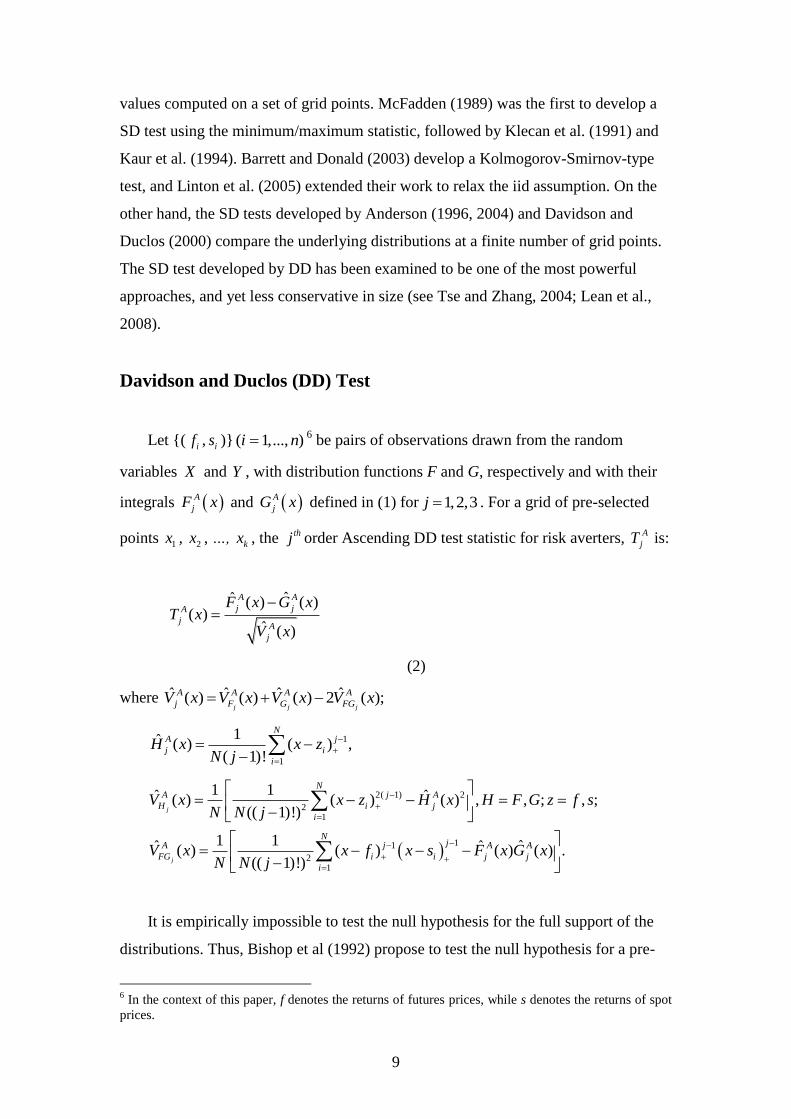
Davidson and Duclos (DD) Test

Let {( if , is )} ( 1,..., )i n6 be pairs of observations drawn from the random

variables X and Y , with distribution functions F and G, respectively and with their

integrals A

jF x and A

jG x defined in (1) for 1,2,3j . For a grid of pre-selected

points 1 x , 2 x , …, kx , the thj order Ascending DD test statistic for risk averters, A

jT is:

ˆˆ ( ) ( )( )

ˆ ( )

A A

j jA

jA

j

F x G xT x

V x

(2)

where ˆ ˆ ˆ ˆ( ) ( ) ( ) 2 ( );j j j

A A A A

j F G FGV x V x V x V x

1

1

1ˆ ( ) ( ) ,( 1)!

NA j

j i

i

H x x zN j

2( 1) 2

21

11

21

1 1ˆ ˆ( ) ( ) ( ) , , ; , ;(( 1)!)

1 1 ˆˆ ˆ( ) ( ) ( ) ( ) .(( 1)!)

j

j

NA j A

H i j

i

NjA j A A

FG i i j j

i

V x x z H x H F G z f sN N j

V x x f x s F x G xN N j

It is empirically impossible to test the null hypothesis for the full support of the

distributions. Thus, Bishop et al (1992) propose to test the null hypothesis for a pre-

6 In the context of this paper, f denotes the returns of futures prices, while s denotes the returns of spot

prices.

10

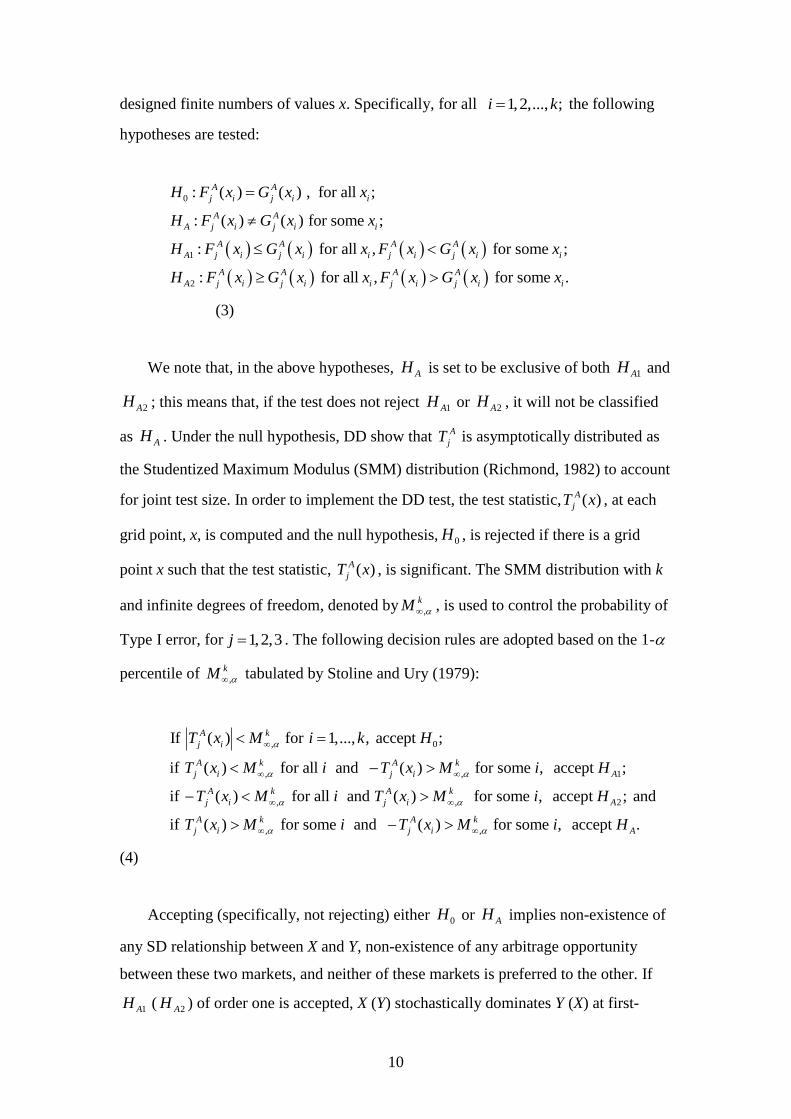
designed finite numbers of values x. Specifically, for all 1,2,..., ;i k the following

hypotheses are tested:

0

1

2

: ( ) ( ) , for all ;

: ( ) ( ) for some ;

: for all , for some ;

: for all , for some .

A A

j i j i i

A A

A j i j i i

A A A A

A j i j i i j i j i i

A A A A

A j i j i i j i j i i

H F x G x x

H F x G x x

H F x G x x F x G x x

H F x G x x F x G x x

(3)

We note that, in the above hypotheses, AH is set to be exclusive of both 1AH and

2AH ; this means that, if the test does not reject 1AH or 2AH , it will not be classified

as AH . Under the null hypothesis, DD show that A

jT is asymptotically distributed as

the Studentized Maximum Modulus (SMM) distribution (Richmond, 1982) to account

for joint test size. In order to implement the DD test, the test statistic, ( )A

jT x , at each

grid point, x, is computed and the null hypothesis, 0H , is rejected if there is a grid

point x such that the test statistic, ( )A

jT x , is significant. The SMM distribution with k

and infinite degrees of freedom, denoted by kM , , is used to control the probability of

Type I error, for 1,2,3j . The following decision rules are adopted based on the 1-

percentile of kM , tabulated by Stoline and Ury (1979):

, 0

, , 1

, , 2

,

If ( ) for 1,..., , accept ;

if ( ) for all and ( ) for some , accept ;

if ( ) for all and ( ) for some , accept ; and

if ( )

A k

j i

A k A k

j i j i A

A k A k

j i j i A

A k

j i

T x M i k H

T x M i T x M i H

T x M i T x M i H

T x M

, for some and ( ) for some , accept .A k

j i Ai T x M i H

(4)

Accepting (specifically, not rejecting) either 0H or AH implies non-existence of

any SD relationship between X and Y, non-existence of any arbitrage opportunity

between these two markets, and neither of these markets is preferred to the other. If

1AH ( 2AH ) of order one is accepted, X (Y) stochastically dominates Y (X) at first-

11

order. In this situation, and under certain regularity conditions7, an arbitrage

opportunity exists, and any non-satiated investors will be better off if they switch

from the dominated asset to the dominant one. On the other hand, if 1AH ( 2AH ) is

accepted for order two (three), a particular market stochastically dominates the other

at second- (third-) order. In this situation, an arbitrage opportunity does not exist, and

switching from one asset to another will only increase the risk averters’ expected

utility, but not their expected wealth (Jarrow, 1986; Falk and Levy, 1989; Wong et al

2008). These results could be used to infer that market efficiency and market

rationality could still hold in these markets (Bernard and Seyhun, 1997; Larsen and

Resnick, 1999; Sriboonchita et al., 2009).

The DD test compares distributions at a finite number of grid points. Various

studies have examined the choice of grid points. For example, Tse and Zhang (2004)

show that an appropriate choice of k, for reasonably large samples, ranges from 6 to

15. Too few grids will miss information of the distributions between any two

consecutive grids (Barrett and Donald, 2003), and too many grids will violate the

independence assumption required by the SMM distribution (Richmond, 1982). In

order to make the comparisons comprehensive without violating the independence

assumption, we follow Fong et al. (2005, 2008), Gasbarro et al (2007) and Lean et al.

(2007) to make 10 major partitions, with 10 minor partitions within any two

consecutive major partitions in each comparison, and base statistical inference on the

SMM distribution for k=10 and infinite degrees of freedom8. This allows the

consistency of both the magnitude and sign of the DD statistics between any two

consecutive major partitions to be examined.

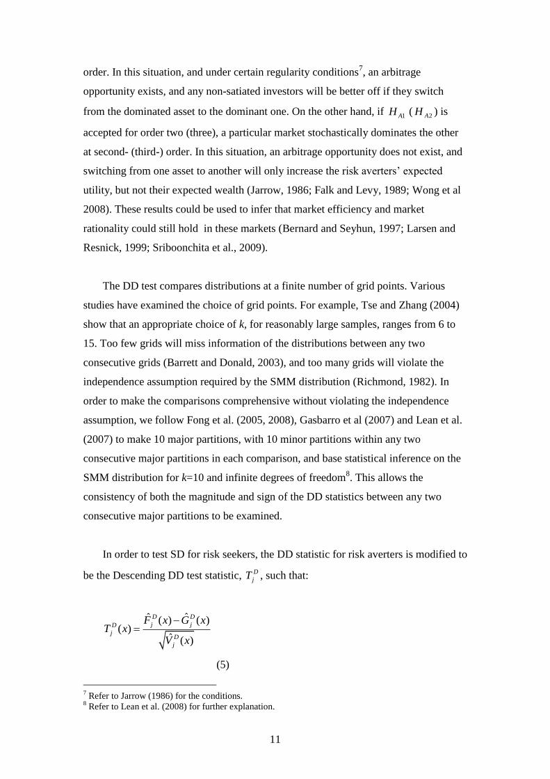
In order to test SD for risk seekers, the DD statistic for risk averters is modified to

be the Descending DD test statistic, D

jT , such that:

ˆˆ ( ) ( )( )

ˆ ( )

D D

j jD

jD

j

F x G xT x

V x

(5)

7 Refer to Jarrow (1986) for the conditions.

8 Refer to Lean et al. (2008) for further explanation.

12

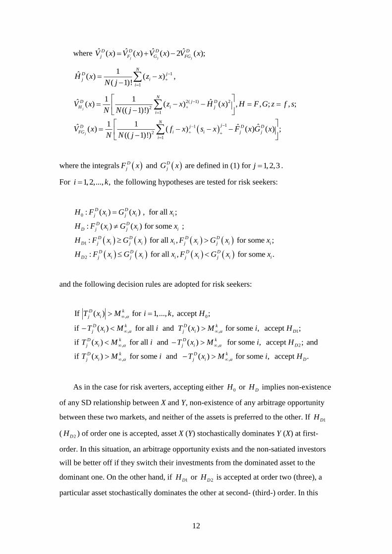
where ˆ ˆ ˆ ˆ( ) ( ) ( ) 2 ( );j j j

D D D D

j F G FGV x V x V x V x

1

1

1ˆ ( ) ( ) ,( 1)!

ND j

j i

i

H x z xN j

2( 1) 2

21

11

21

1 1ˆ ˆ( ) ( ) ( ) , , ; , ;(( 1)!)

1 1 ˆˆ ˆ( ) ( ) ( ) ( ) ;(( 1)!)

j

j

ND j D

H i j

i

NjD j D D

FG i i j j

i

V x z x H x H F G z f sN N j

V x f x s x F x G xN N j

where the integrals D

jF x and D

jG x are defined in (1) for 1,2,3j .

For 1,2,..., ,i k the following hypotheses are tested for risk seekers:

0

1

2

: ( ) ( ) , for all ;

: ( ) ( ) for some ;

: for all , for some ;

: for all , for some .

D D

j i j i i

D D

D j i j i i

D D D D

D j i j i i j i j i i

D D D D

D j i j i i j i j i i

H F x G x x

H F x G x x

H F x G x x F x G x x

H F x G x x F x G x x

and the following decision rules are adopted for risk seekers:

, 0

, , 1

, , 2

,

If ( ) for 1,..., , accept ;

if ( ) for all and ( ) for some , accept ;

if ( ) for all and ( ) for some , accept ; and

if ( )

D k

j i

D k D k

j i j i D

D k D k

j i j i D

D k

j i

T x M i k H

T x M i T x M i H

T x M i T x M i H

T x M

, for some and ( ) for some , accept .D k

j i Di T x M i H

As in the case for risk averters, accepting either 0H or DH implies non-existence

of any SD relationship between X and Y, non-existence of any arbitrage opportunity

between these two markets, and neither of the assets is preferred to the other. If 1DH

( 2DH ) of order one is accepted, asset X (Y) stochastically dominates Y (X) at first-

order. In this situation, an arbitrage opportunity exists and the non-satiated investors

will be better off if they switch their investments from the dominated asset to the

dominant one. On the other hand, if 1DH or 2DH is accepted at order two (three), a

particular asset stochastically dominates the other at second- (third-) order. In this

13

situation, an arbitrage opportunity does not exist, and switching from one asset to

another will only increase the risk seekers’ expected utility, but not expected wealth.

Empirical Results and Discussion

[Table 1 here]

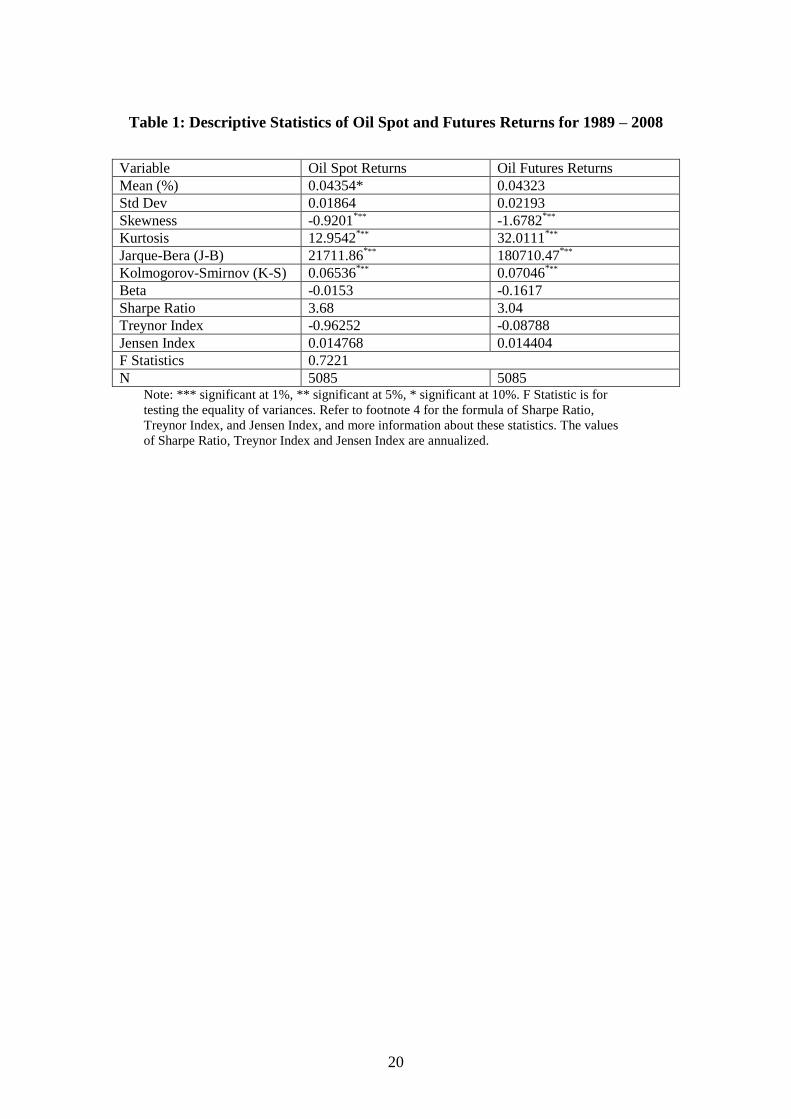
Table 1 provides the descriptive statistics for the daily returns of oil spot prices

and oil futures prices for the entire sample period. The means of their daily returns are

about 0.04%, significant at 10% for oil spot but not significant for oil futures. From

the unreported paired t-test, the mean return of oil spot is insignificantly higher than

that of futures whereas, as expected, its standard deviation is not significantly smaller

than that of futures. As the means and standard deviations are not significantly

different for the two returns, the MV criterion is unable to indicate any preference

between these two assets.

For the CAPM measures, the beta (absolute value) of oil spot return is smaller

than that of futures; both being negative and less than one. Both returns have similar

Sharpe ratios, Treynor and Jensen indices, with no significant difference between the

returns for each statistic. Thus, the information drawn from the CAPM statistics

cannot lead to any preference between the spot and futures prices. In addition, the

highly significant Kolmogorov-Smirnov (K-S) and Jarque-Bera (J-B) statistics shown

in Table 1 indicate that both returns are non-normal.9 Moreover, both daily returns are

negatively skewed. As expected, oil futures have much higher kurtosis than spot, with

both being higher than that under normality. Both significant skewness and kurtosis

indicate non-normality in the returns distributions, and thus lead to the conclusion that

the normality requirement in the traditional MV and CAPM measures is violated.

SD Analysis for Risk Averters

[Figure 1 here]

9 The results of other normality tests, such as Shapiro-Wilk, lead to the same conclusion. The results

are available on request.

14

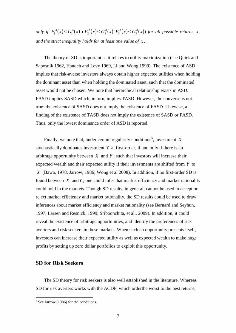
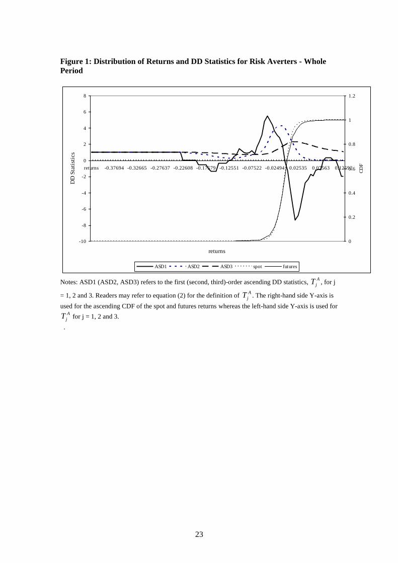
We first depict the CDFs of the returns for both oil spot and futures prices and

their corresponding first three orders of the Ascending DD statistics, A

jT , for risk

averters in Figure 1. If oil futures dominate spot in the sense of FASD, then the CDF

of futures returns should lie significantly below that of spot for the entire range.

However, Figure 1 shows that the CDF of spot lies below that of futures in the

downside risk, while the CDF of futures lies below that of spot on the upside profit.

This indicates that there could be no FASD between the two returns and that spot

could dominate futures on the downside risk, while futures could dominate spot on the

upside profit range. In order to verify this finding formally, we employ the first three

orders of the Ascending DD statistics, A

jT ( 1,2,3j ), for the two series, with the

results reported in Table 2. DD states that the null hypothesis can be rejected if any of

the test statistics A

jT is significant with the wrong sign.

[Table 2 here]

The values of 1

AT depicted in Figure 1 move from positive to negative along the

distribution of returns, together with the percentage of significant values reported in

Table 2, show that 5% of 1

AT is significantly positive, whereas 6% of it is

significantly negative. Thus, the hypotheses that futures stochastically dominate spot,

or vice-versa, at first-order are rejected, implying that no arbitrage opportunity exists

between these two series. We can, however, state that oil spot dominates futures

marginally in the downside returns, while oil futures dominate spot marginally in the

upside profit.

The SD criterion enables us to compare utility interpretations in terms of

investors’ risk aversion and decreasing absolute risk aversion, respectively, by

examining the higher order SD relationships. The Ascending DD statistics, 2

AT and

3

AT , depicted in Figure 1 are positive in the entire range of the returns distribution,

with 7% of 2

AT (5% of 3

AT ) being significantly positive and no 2

AT ( 3

AT ) being

significantly negative. This implies that oil spot marginally SASD (TASD) dominates

15

futures, and hence risk-averse investors would prefer investing in oil spot than futures

to maximize their expected utility.

Will Risk Seekers Have Different Preferences?

So far, if we apply the existing ASD tests, we could only draw conclusions

regarding the preference of risk-averse investors, but not of risk seekers. Nonetheless,

the result also shows that futures dominate spot for the upside profit. However,

applying the ASD test alone could not yield any inference based on this information.

Thus, an extension of the SD test for risk seekers is necessary, as discussed in

previous sections. Subsequent discussions illustrate the applicability of the DSD test

for risk seekers in this section

It is well known that investors could be risk-seeking (see, for example,

Markowitz, 1952; Kahneman and Tversky, 1979; Tversky and Kahneman, 1992;

Levy and Levy, 2004; Post and Levy, 2005). In order to examine the risk-seeking

behavior, DSD theory for risk-seeking has been developed. In this paper, we put the

theory into practice by extending the DD test for risk seekers, namely Descending DD

statistics, D

jT ( j = 1, 2 and 3), of the first three orders for risk seekers, with the

correspondence statistics as discussed in the previous section.

[Figure 2 here]

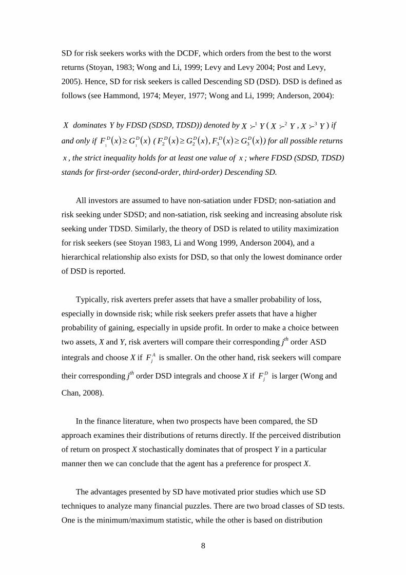
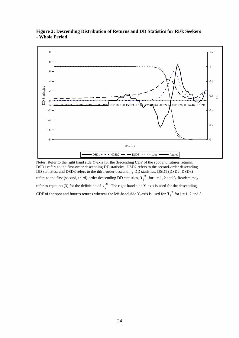
Figure 2 shows the descending cumulative density functions (DCDFs) for the

daily returns of both oil spot and futures prices over the entire distribution range for

the whole sample period. The cross of the two DCDFs suggests that there is no FDSD

between futures and spot returns. The DCDF of the futures lies above that of spot for

the upside profit, while the DCDF of the spot lies above that of futures for the

downside risk. This indicates that futures could be preferred to spot for upside profit,

while spot could be preferred to futures for downside risk.

[Table 3 here]

16

In order to test this phenomenon formally, we plot the Descending DD statistics,

D

jT , of the first three orders in Figure 2, and report the percentages of their significant

positive and negative portions in Table 3. Figure 2 shows that 1

DT is positive in the

upside profit range and negative in the downside risk range, whereas Table 3 shows

that 6% (5%) of the positive (negative) values of 1

DT is significant. This indicates that

there is no FDSD relationship between the two series for the entire period.

As there is no FDSD, we examine the D

jT for the second and third orders. Both

2

DT and 3

DT depicted in Figure 2 are positive for the entire range, implying that risk-

seeking investors could prefer futures to spot. In order to verify this statement

statistically, we use the results in Table 3 that 7% (9%) of 2

DT ( 3

DT ) are significantly

positive, while no 2

DT ( 3

DT ) is significantly negative. This leads us to conclude

statistically that the oil futures SDSD and TDSD the oil spot and consequently, risk-

seeking investors, prefer oil futures to spot to maximize their utility.

In addition, neither FASD nor FDSD leads us to conclude that market efficiency

or market rationality could hold in the oil spot and futures markets. The preferences of

risk-averse and risk-seeking investors towards spot and futures do not violate market

inefficiency, unless the oil market has only one type of investors. Our results are

consistent with existing results in the literature, for example, Fong et al. (2005), who

examine momentum profits in stocks markets.

The Impact of Oil Crises

The oil market is very sensitive, not only to news, but also to the expectation of news

(Maslyuk and Smyth, 2008). For example, when the OPEC countries agreed to reduce

the combined production of crude oil in 1999, oil prices increased further. Similarly,

the Iraq War (that is, the Second Gulf War) occurred in March 2003. This caused oil

futures prices to increase further due to the fear that Iraq’s oil fields and pipelines

might be destroyed during the war. We employ regression analysis, with the cut-off

points of the crises being stated in the previous section, as dummies and find that the

dummies affect both spot and futures in the Iraq war crisis, but not in the OPEC crisis.

17

This indicates that the war’s impact is greater for both spot and futures markets.10

On

the other hand, it is of interest to examine the effects of these oil crises while

comparing the performances of oil spot and futures markets and the investors’

preferences in these markets. To this end, we employ the SD tests to analyse the

return series for the pre- and OPEC, and pre- and Iraq-War, sub-periods.

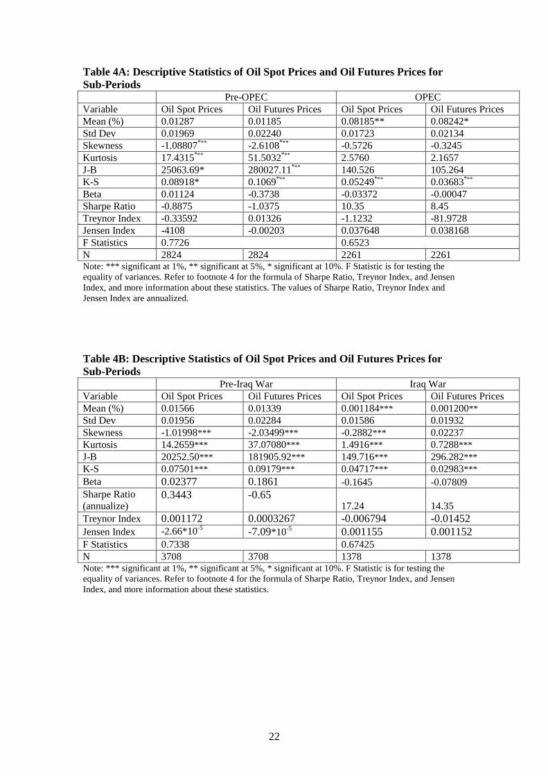
[Table 4 here]

Tables 4A and 4B provide descriptive statistics of the daily returns of oil spot and

futures prices for the OPEC and Iraq War sub-periods. As most of the results of the

MV criterion and CAPM statistics for the sub-periods are similar to those for the

entire full sample period, we will only discuss those results that are different from the

full sample period. However, compared with the pre-OPEC sub-period, the means for

both spot and futures returns in the OPEC sub-period dramatically increased five-fold.

On the other hand, compared with the pre-Iraq-War sub-period, both spot and futures

returns in the Iraq-War sub-period were reduced by 90%. Nonetheless, the difference

between the means of spot and futures in each sub-period is still not significant. In

addition, the standard deviations for the returns of spot and futures are also not

significantly different in each of the sub-periods. Thus, similar to the inference for the

entire sample, both the MV criterion and the CAPM statistics are unable to indicate

any dominance between the spot and futures markets.

We turn to the SD tests to conduct the analysis. From the DD test, we find that all

values of A

jT and D

jT (j = 1, 2 and 3) for both risk averters and risk seekers are not

significant at the 5% level for the first three orders in the pre-OPEC sub-period.

Therefore, there is no arbitrage opportunity in these markets. and both risk averters

and risk seekers are indifferent between these two indices in the pre-OPEC sub-

period. However, in the OPEC sub-period, Table 2 shows that 17% (16%) of 2

AT ( 3

AT )

are significantly positive. and none of the 2

AT ( 3

AT ) is significantly negative, while

Table 3 reveals that 22% (30%) of 2

DT ( 3

DT ) are significantly positive and none of the

2

DT ( 3

DT ) is significantly negative at the 5% level. Similar inferences can be drawn for

10

We do not report these results, which are available on request.

18

the Iraq War sub-period. Hence, we conclude that, compared with the full sample

period, the risk-averse investors prefer the spot index more, and risk seekers are

attracted to the futures index more to maximize their expected utility, but not their

expected wealth, in both the OPEC and Iraq War sub-periods.

Conclusions

This paper offered a robust decision tool for investment decisions with

uncertainty to the oil markets. The SD tests enabled us to reveal the existence of

arbitrage opportunities, identify the preferences for both risk averters and risk seekers

over different investment prospects, and enable us to make inference on market

rationality and market efficiency. We developed the SD tests of DD for risk seekers,

and applied the DD tests to examine the behavior of both risk averters and risk

seekers with regard to oil spot and futures markets, and compared the performance

between these two markets.

Our results showed conclusively that oil spot dominates oil futures on the

downside risk, whereas the futures dominate spot on the upside profit range. We

concluded that there is neither arbitrage opportunity nor preference being prevalent

between these two indices for both risk-averse and risk-seeking investors in the pre-

AFC sub-period. However, risk-averse investors prefer the oil spot, while risk seekers

are attracted to the oil future in order to maximize their expected utility in the post-

AFC sub-period.

We note that some authors have proposed to use higher order (higher than three)

SD in empirical applications. For example, Vinod (2004) recommends employing 4th

order SD to make the choice among investment prospects, with an illustration of 1281

mutual funds. We also note that the most commonly-used orders in SD for empirical

analyses, regardless of whether they are simple or complicated, are the first three, and

one could easily extend the theory developed in this paper to any order.

It should be noted that many studies have claimed that if the normality

assumption fails, the results drawn using the MV criterion and CAPM statistics can be

19

misleading. We point out that, unlike the SD approach that is consistent with utility

maximisation, the dominance findings using the MV and CAPM measures may only

be consistent with utility maximization, if the asset returns are not normally

distributed, under very specific conditions. For example, Meyer (1977), Wong (2006,

2007) and Wong and Ma (2008) show that, if the returns of two assets follow the

same location-scale family, then an MV domination could infer preferences by risk

averters on the dominant fund to the dominated one.

Finally, if all of the regularity conditions are satisfied (for example, assets

follow the normality assumption), the MV and CAPM measures be consistent if asset

returns possess the second order SD preference characteristic. However, even if all of

the regularity conditions are satisfied, the MV and CAPM measures cannot identify

the situations in which one fund dominates another at first or third order SD. Thus, the

SD approach allows more accurate and useful assessments for financial assets,

regardless of whether those returns are normally or non-normally distributed.

20

Table 1: Descriptive Statistics of Oil Spot and Futures Returns for 1989 – 2008

Variable Oil Spot Returns Oil Futures Returns

Mean (%) 0.04354* 0.04323

Std Dev 0.01864 0.02193

Skewness -0.9201*** -1.6782

***

Kurtosis 12.9542*** 32.0111

***

Jarque-Bera (J-B) 21711.86*** 180710.47

***

Kolmogorov-Smirnov (K-S) 0.06536*** 0.07046

***

Beta -0.0153 -0.1617

Sharpe Ratio 3.68 3.04

Treynor Index -0.96252 -0.08788

Jensen Index 0.014768 0.014404

F Statistics 0.7221

N 5085 5085 Note: *** significant at 1%, ** significant at 5%, * significant at 10%. F Statistic is for

testing the equality of variances. Refer to footnote 4 for the formula of Sharpe Ratio,

Treynor Index, and Jensen Index, and more information about these statistics. The values

of Sharpe Ratio, Treynor Index and Jensen Index are annualized.

21

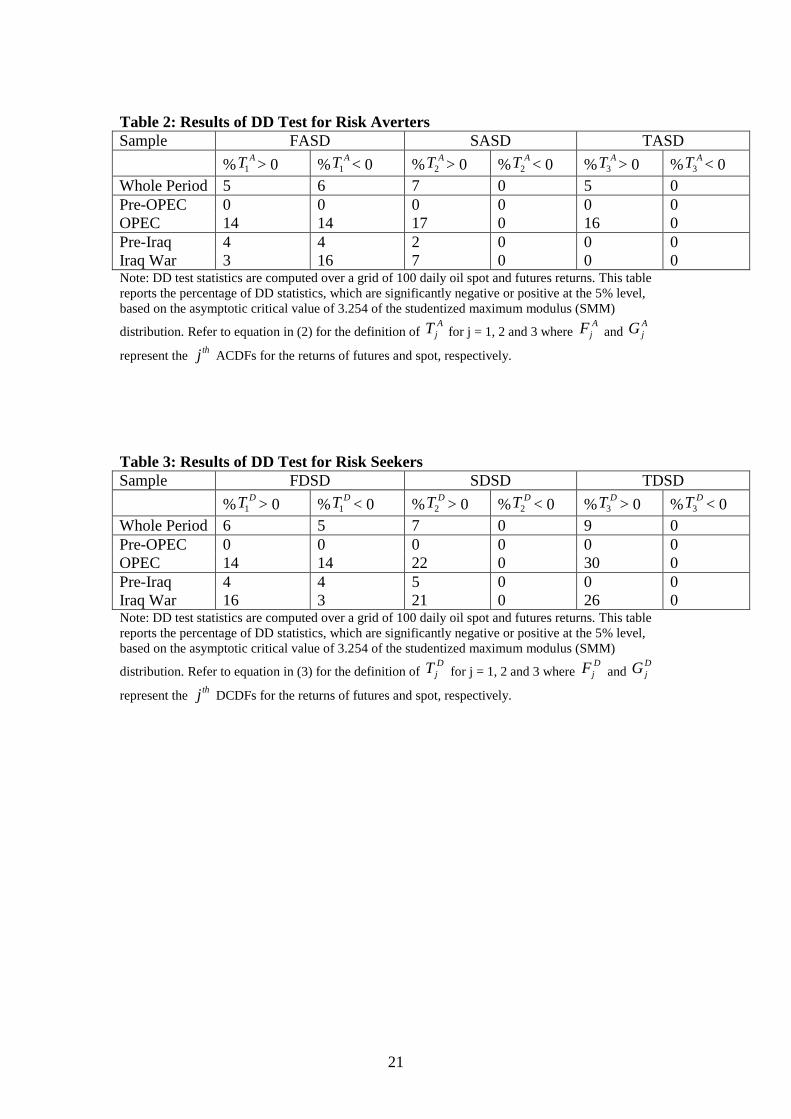
Table 2: Results of DD Test for Risk Averters

Sample FASD SASD TASD

% 1

AT > 0 % 1

AT < 0 % 2

AT > 0 % 2

AT < 0 % 3

AT > 0 % 3

AT < 0

Whole Period 5 6 7 0 5 0

Pre-OPEC 0 0 0 0 0 0

OPEC 14 14 17 0 16 0

Pre-Iraq 4 4 2 0 0 0

Iraq War 3 16 7 0 0 0 Note: DD test statistics are computed over a grid of 100 daily oil spot and futures returns. This table

reports the percentage of DD statistics, which are significantly negative or positive at the 5% level,

based on the asymptotic critical value of 3.254 of the studentized maximum modulus (SMM)

distribution. Refer to equation in (2) for the definition of A

jT for j = 1, 2 and 3 where A

jF and A

jG

represent the thj ACDFs for the returns of futures and spot, respectively.

Table 3: Results of DD Test for Risk Seekers

Sample FDSD SDSD TDSD

% 1

DT > 0 % 1

DT < 0 % 2

DT > 0 % 2

DT < 0 % 3

DT > 0 % 3

DT < 0

Whole Period 6 5 7 0 9 0

Pre-OPEC 0 0 0 0 0 0

OPEC 14 14 22 0 30 0

Pre-Iraq 4 4 5 0 0 0

Iraq War 16 3 21 0 26 0 Note: DD test statistics are computed over a grid of 100 daily oil spot and futures returns. This table

reports the percentage of DD statistics, which are significantly negative or positive at the 5% level,

based on the asymptotic critical value of 3.254 of the studentized maximum modulus (SMM)

distribution. Refer to equation in (3) for the definition of D

jT for j = 1, 2 and 3 where D

jF and D

jG

represent the thj DCDFs for the returns of futures and spot, respectively.

22

Table 4A: Descriptive Statistics of Oil Spot Prices and Oil Futures Prices for

Sub-Periods Pre-OPEC OPEC

Variable Oil Spot Prices Oil Futures Prices Oil Spot Prices Oil Futures Prices

Mean (%) 0.01287 0.01185 0.08185** 0.08242*

Std Dev 0.01969 0.02240 0.01723 0.02134

Skewness -1.08807*** -2.6108

*** -0.5726 -0.3245

Kurtosis 17.4315*** 51.5032

*** 2.5760 2.1657

J-B 25063.69* 280027.11*** 140.526 105.264

K-S 0.08918* 0.1069*** 0.05249

*** 0.03683***

Beta 0.01124 -0.3738 -0.03372 -0.00047

Sharpe Ratio -0.8875 -1.0375 10.35 8.45

Treynor Index -0.33592 0.01326 -1.1232 -81.9728

Jensen Index -4108

-0.00203

0.037648 0.038168

F Statistics 0.7726 0.6523

N 2824 2824 2261 2261 Note: *** significant at 1%, ** significant at 5%, * significant at 10%. F Statistic is for testing the

equality of variances. Refer to footnote 4 for the formula of Sharpe Ratio, Treynor Index, and Jensen

Index, and more information about these statistics. The values of Sharpe Ratio, Treynor Index and

Jensen Index are annualized.

Table 4B: Descriptive Statistics of Oil Spot Prices and Oil Futures Prices for

Sub-Periods Pre-Iraq War Iraq War

Variable Oil Spot Prices Oil Futures Prices Oil Spot Prices Oil Futures Prices

Mean (%) 0.01566 0.01339 0.001184*** 0.001200**

Std Dev 0.01956 0.02284 0.01586 0.01932

Skewness -1.01998*** -2.03499*** -0.2882*** 0.02237

Kurtosis 14.2659*** 37.07080*** 1.4916*** 0.7288***

J-B 20252.50*** 181905.92*** 149.716*** 296.282***

K-S 0.07501*** 0.09179*** 0.04717*** 0.02983***

Beta 0.02377 0.1861 -0.1645 -0.07809

Sharpe Ratio

(annualize) 0.3443 -0.65

17.24 14.35

Treynor Index 0.001172 0.0003267 -0.006794 -0.01452

Jensen Index -2.66*10-5

-7.09*10-5 0.001155 0.001152

F Statistics 0.7338 0.67425

N 3708 3708 1378 1378 Note: *** significant at 1%, ** significant at 5%, * significant at 10%. F Statistic is for testing the

equality of variances. Refer to footnote 4 for the formula of Sharpe Ratio, Treynor Index, and Jensen

Index, and more information about these statistics.

23

Figure 1: Distribution of Returns and DD Statistics for Risk Averters - Whole

Period

-10

-8

-6

-4

-2

0

2

4

6

8

returns -0.37694 -0.32665 -0.27637 -0.22608 -0.17579 -0.12551 -0.07522 -0.02494 0.02535 0.07563 0.12592

returns

DD

Sta

tist

ics

0

0.2

0.4

0.6

0.8

1

1.2

CD

F

ASD1 ASD2 ASD3 spot futures

Notes: ASD1 (ASD2, ASD3) refers to the first (second, third)-order ascending DD statistics,

A

jT , for j

= 1, 2 and 3. Readers may refer to equation (2) for the definition of A

jT . The right-hand side Y-axis is

used for the ascending CDF of the spot and futures returns whereas the left-hand side Y-axis is used for A

jT for j = 1, 2 and 3.

.

24

Figure 2: Descending Distribution of Returns and DD Statistics for Risk Seekers

- Whole Period

-8

-6

-4

-2

0

2

4

6

8

10

returns -0.38252 -0.33783 -0.29313 -0.24843 -0.20373 -0.15903 -0.11433 -0.06964 -0.02494 0.01976 0.06446 0.10916

returns

DD

Sta

tist

ics

0

0.2

0.4

0.6

0.8

1

1.2

CD

F

DSD1 DSD2 DSD3 spot futures

Notes: Refer to the right hand side Y-axis for the descending CDF of the spot and futures returns.

DSD1 refers to the first-order descending DD statistics; DSD2 refers to the second-order descending

DD statistics; and DSD3 refers to the third-order descending DD statistics. DSD1 (DSD2, DSD3)

refers to the first (second, third)-order descending DD statistics, D

jT , for j = 1, 2 and 3. Readers may

refer to equation (3) for the definition of D

jT . The right-hand side Y-axis is used for the descending

CDF of the spot and futures returns whereas the left-hand side Y-axis is used for D

jT for j = 1, 2 and 3.

25

References

Anderson, G.., 1996. Nonparametric tests of stochastic dominance in income

distributions. Econometrica 64, 1183 – 1193.

Anderson, G.., 2004. Toward an empirical analysis of polarization. Journal of

Econometrics 122, 1-26.

Bai, Z.D., Liu, H.X., Wong, W.K., 2009a. Enhancement of the Applicability of

Markowitz's Portfolio Optimization by Utilizing Random Matrix Theory.

Mathematical Finance 19(4), 639-667.

Bai, Z.D., Liu, H.X., Wong, W.K., 2009b. On the Markowitz Mean-Variance

Analysis of Self-Financing Portfolios, Risk and Decision Analysis 1(1), 35-42.

Barrett, G., Donald, S., 2003. Consistent tests for stochastic dominance. Econometrica

71, 71-104.

Bawa, V.S., 1978. Safety-first, stochastic dominance, and optimal portfolio choice.

Journal of Financial and Quantitative Analysis 13, 255-271.

Beedles, W.L. 1979. Return, dispersion and skewness: synthesis and investment

strategy. Journal of Financial Research 2, 71-80.

Bekiros, S.D., Diks, C.G.H., 2008. The Relationship between Crude Oil Spot and

Futures Prices: Cointegration, Linear and Nonlinear Causality. Energy Economics

30(5), 2673-2685.

Bernard, V.L., Seyhun, H.N., 1997. Does post-earnings-announcement drift in stock

prices reflect a market inefficiency? A stochastic dominance approach. Review of

Quantitative Finance and Accounting 9, 17-34.

Bishop, J.A., Formly, J.P., Thistle, P.D., 1992. Convergence of the South and non-

South income distributions. American Economic Review 82, 262-272.

Bopp, A.E., Sitzer, S., 1987. Are petroleum futures prices good predictors of cash

value? Journal of Futures Markets 7, 705-719.

Crowder, W.J., Hamid, A., 1993. A co-integration test for oil futures market

efficiency. Journal of Futures Markets 13, 933-941.

Cumby, R.E., Glen, J.D., 1990. Evaluating the performance of international mutual

funds. Journal of Finance 45(2), 497-521.

Davidson, R., Duclos, J-Y., 2000. Statistical inference for stochastic dominance and

for the measurement of poverty and inequality. Econometrica 68, 1435-1464.

Egozcue, M., Wong, W.K., 2010. Gains from diversification: A majorization and

stochastic dominance approach. European Journal of Operational Research 200, 893–

900.

26

Falk, H., Levy, H., 1989. Market reaction to quarterly earnings' announcements: A

stochastic dominance based test of market efficiency. Management Science 35, 425-

446.

Fishburn, P.C., 1964. Decision and Value Theory, New York.

Fong, W.M., Lean, H.H., Wong, W.K., 2008. Stochastic dominance and behavior

towards risk: the market for internet stocks. Journal of Economic Behavior and

Organization 68(1), 194-208.

Fong, W.M., See, K.H., 2002. A Markov switching model of the conditional volatility

of crude oil futures prices. Energy Economics 24, 71-95.

Fong, W.M., See, K.H., 2003. Basis variations and regime shifts in the oil futures

market. The European Journal of Finance 9, 499–513.

Fong, W.M., Lean, H.H., Wong, W.K., 2008. Stochastic dominance and behavior

towards risk: the market for Internet stocks. Journal of Economic Behavior and

Organization 68(1), 194-208.

Fong, W.M., Wong, W.K., Lean, H.H., 2005. International momentum strategies: A

stochastic dominance approach. Journal of Financial Markets 8, 89–109.

Gasbarro, D., Wong, W.K., Zumwalt, J.K., 2007. Stochastic dominance analysis of

iShares. European Journal of Finance 13, 89-101.

Gulen, S.G., 1999. Regionalization in world crude oil markets: further evidence.

Energy Journal 20, 125-139.

Hadar J., Russell, W.R., 1969. Rules for ordering uncertain prospects. American

Economic Review 59, 25-34.

Hammond, J.S., 1974. Simplifying the choice between uncertain prospects where

preference is nonlinear. Management Science 20(7), 1047-1072.

Hammoudeh, S., Li, H., Jeon, B., 2003. Causality and volatility spillovers among

petroleum prices of WTI, gasoline and heating oil in different locations. North

American Journal of Economics and Finance 14, 89-114.

Hammoudeh, S., Li, H., 2004. The impact of the Asian crisis on the behavior of US

and international petroleum prices. Energy Economics 26, 135–160.

Hanoch, G., Levy, H., 1969. The efficiency analysis of choices involving risk. Review

of Economic studies 36, 335-346.

Jarrow, R., 1986. The relationship between arbitrage and first order stochastic

dominance. Journal of Finance 41, 915-921.

27

Jensen, M.C., 1969. Risk, the pricing of capital assets and the evaluation of

investment portfolios. Journal of Business 42, 167-247.

Kahneman, D., Tversky, A., 1979. Prospect theory of decisions under risk,

Econometrica 47(2), 263-291.

Kaur, A., Rao, B.L.S.P., Singh, H., 1994. Testing for second order stochastic

dominance of two distributions. Econometric Theory 10, 849 – 866.

Klecan, L., McFadden, R., McFadden, D., 1991. A robust test for stochastic

dominance. Working Paper, MIT & Cornerstone Research.

Larsen G.A., Resnick, B.G.., 1999. A performance comparison between cross-

sectional stochastic dominance and traditional event study methodologies. Review of

Quantitative Finance and Accounting 12, 103-112.

Lean, H.H., Smyth, R., Wong, W.K., 2007. Revisiting calendar anomalies in Asian

stock markets using a stochastic dominance approach. Journal of Multinational

Financial Management 17(2), 125–141.

Lean, H.H., Wong, W.K., Zhang, X., 2008. Size and Power of Some Stochastic

Dominance Tests: A Monte Carlo Study, Mathematics and Computers in Simulation

79, 30-48.

Leung, P.L., Wong, W.K., 2008. On Testing the Equality of the Multiple Sharpe

Ratios, with Application on the Evaluation of IShares. Journal of Risk 10(3), 1-16.

Levy, H., Levy, M., 2004. Prospect theory and mean-variance analysis. Review of

Financial Studies 17(4), 1015-1041.

Li, C.K., Wong, W.K., 1999. A note on stochastic dominance for risk averters and

risk takers. RAIRO Recherche Operationnelle 33, 509-524.

Lin, X.S., Tamvakis, M.N., 2001. Spillover effects in energy futures markets. Energy

Economics 23, 43-56.

Linton, O., Maasoumi, E., Whang, Y-J., 2005. Consistent testing for stochastic

dominance under general sampling schemes. Review of Economic Studies 72, 735-

765.

Markowitz, H.M., 1952. Portfolio selection. Journal of Finance 7, 77-91.

McFadden, D., 1989. Testing for stochastic dominance. In: T.B. Fomby and T.K. Seo,

(Eds.), Studies in the Economics of Uncertainty. Springer Verlag, New York.

Meyer, J., 1977. Second degree stochastic dominance with respect to a function.

International Economic Review 18, 476-487.

28

Morey, M.R., Morey, R.C. 2000. An analytical confidence interval for the Treynor

index: formula, conditions and properties. Journal of Business Finance & Accounting

27(1) & (2), 127-154.

Post, T., Levy, H., 2005. Does risk seeking drive asset prices? A stochastic dominance

analysis of aggregate investor preferences and beliefs. Review of Financial Studies

18(3), 925-953.

Quan, J., 1992. Two step testing procedure for price discovery role of futures prices.

Journal of Futures Markets 12, 139-149.

Quirk J.P., Saposnik, R., 1962. Admissibility and measurable utility functions.

Review of Economic Studies 29, 140-146.

Richmond, J., 1982. A general method for constructing simultaneous confidence

intervals. Journal of the American Statistical Association 77, 455-460.

Rochschild, M., Stiglitz, J.E., 1970. Increasing risk I. A definition. Journal of

Economic Theory 2, 225-243.

Schwartz, T.V., Szakmary, A.C., 1994. Price discovery in petroleum markets:

arbitrage, cointegration and the time interval of analysis. Journal of Futures Markets

14, 147-167.

Schwert, G., William, 1990. Stock returns and real activity: a century of evidence.

Journal of Finance 45(4), 1237-1257.

Serletis, A., Banack, D., 1990. Market efficiency and co-integration: an application to

petroleum markets. Review of Futures Markets 9, 372-385.

Sharpe, W.F., 1964. Capital asset prices: Theory of market equilibrium under

conditions of risk. Journal of Finance 19, 425-442.

Silvapulle, P., Moosa I., 1999. The relationship between spot and futures prices:

evidence from the crude oil market. Journal of Futures Markets 19, 175-193.

Sriboonchita, S., Wong, W.K., Dhompongsa, S., Nguyen, H.T., 2009. Stochastic

Dominance and Applications to Finance, Risk and Economics, Chapman and

Hall/CRC, Taylor and Francis Group, Boca Raton, Florida, USA.

Stoline, M.R., Ury, H.K., 1979. Tables of the studentized maximum modulus

distribution and an application to multiple comparisons among means. Technometrics

21, 87-93.

Stoyan, D., 1983. Comparison methods for queues and other stochastic models. New

York: Wiley.

Tesfatsion, L., 1976. Stochastic dominance and maximization of expected utility.

Review of Economic Studies 43, 301-315.

29

Tobin, J., 1958. Liquidity preference and behavior towards risk. Review of Economic

Studies 25, 65-86.

Treynor, J.L., 1965. How to rate management of investment funds. Harvard Business

Review 43, 63-75.

Tse, Y.K., Zhang, X., 2004. A Monte Carlo investigation of some tests for stochastic

dominance. Journal of Statistical Computation and Simulation 74, 361-378.

Tversky, A., Kahneman, D., 1992. Advances in prospect theory: Cumulative

representation of uncertainty. Journal of Risk and Uncertainty 5, 297-323.

Vinod, H.D., 2004. Ranking mutual funds using unconventional utility theory and

stochastic dominance, Journal of Empirical Finance 11, 353–377.

Wilson, B., Aggarwal, R., Inclan, C., 1996. Detecting volatility changes across the oil

sector. Journal of Futures Markets 16, 313–320.

Wong, W.K., 2006. Stochastic Dominance Theory for Location-Scale Family, Journal

of Applied Mathematics and Decision Sciences 2006, 1-10.

Wong, W.K., 2007. Stochastic dominance and mean-variance measures of profit and

loss for business planning and investment, European Journal of Operational Research

182, 829-843.

Wong, W.K., Chan, R.H., 2008. Markowitz and prospect stochastic dominances,

Annals of Finance 4(1), 105-129.

Wong, W.K., Li, C.K., 1999. A note on convex stochastic dominance theory,

Economics Letters 62, 293-300.

Wong, W.K. Ma, C., 2008. Preferences over location-scale family, Economic

Theory 37(1), 119-146.

Wong, W.K., Phoon, K.F., Lean, H.H., 2008. Stochastic dominance analysis of Asian

hedge funds, Pacific-Basin Finance Journal 16(3), 204-223.