DEPARTMENT OF ECONOMICSUNIVERSITY OF MILAN - BICOCCA

WORKING PAPER SERIES

Occupational Choice, Wealth Distribution and Development

Emilio Colombo, Ákos Valentinyi

No. 25 - September 1999

Dipartimento di Economia Politica Università degli Studi di Milano - Bicocca

http://dipeco.economia.unimib.it

Occupational Choice, Wealth

Distribution and Development �

Emilio Colombo (State University of Milan - Bicocca) y

�Akos Valentinyi (University of Southampton & CEPR)

Abstract

This paper develops a model of occupational choice and income

distribution in which both the wage rate and the interest rate are

determined endogenously. We show the existence of multiple equilibria

that depend on the initial distribution. In particular there can be a

"development trap" characterized by many poor workers earning low

wages and few rich entrepreneurs that exploit the low wage level and

the high interest rate.

�This research has been undertaken with support from the European Union's PhareACE Programme, P96-6151-R.

yAddress for correspondence: Dipartimento di Economia, Facolt�a di Economia, Uni-versit�a Statale Milano - Bicocca, Piazza Ateneo Nuovo 1, Edi�cio u6, 20126, Milano, Italy.Email: Emilio.Colombo@unimi.it

1

1 Introduction

Under many points of view the transition process that is characterizing East-ern Europe, provides an interesting example to test the relevance of di�erenteconomic theory and the e�ects of di�erent policies. What makes this exam-ple interesting is the fact that these economies started the transition fromsimilar initial conditions1, (they had the same industrial structure, geograph-ical location, trading partners and they had similar levels and distributionsof income per capita); yet after only seven years since the beginning of re-forms some economies seem to follow a development path that looks verymuch di�erent from the one followed by others. The question of particularrelevance is whether this is just a temporary phenomenon determined by themassive shock of the fall of the planned system, and therefore sometimesin the future they will all converge to some similar economic conditions, orin fact they are e�ectively taking di�erent development path that will leadthem very much apart from each other.In other words it is important to understand if what we observe is just thetransitional dynamics of a system that displays a unique steady state, or theyare approaches to di�erent equilibria displayed by the same system. Apartfrom the technical point of view this is crucial in terms of policy analysis; inthe former case in fact policy does not matter very much: the best it can bedone is to speed up or slow down the speed of transition to the steady state.In the latter case policy is extremely important: one shot policies in factcan have permanent e�ects and put the economy on a di�erent developmentpath.

The emphasis put in this paper on income distribution is an aspect of par-ticular relevance for transitional economies. One of the results (perhaps theonly one) that was achieved by the socialist system was the realization of avery low degree of inequality in the distribution of income; yet few years af-ter the beginning of transition income inequality has considerably increased.It seems therefore interesting and appropriate, while analyzing the long rundevelopment of those economies, to address also the issue of income distri-bution.The focus on income distribution, moreover, allows to tie the literature ontransitional economies with the more general literature on development eco-nomics that has recently seen a resurgence of interest on themes relatedto distributional aspects. The present paper is related in particular withAghion and Bolton (1997), Banerjee and Newman (1993), Galor and Zeira

1At least considering di�erent groups of economies. i.e. baltic states, central Europe(Hungary, Poland and Czech Republic), NIS etc.

2

(1993) and Piketty (1997); in all those papers it is stressed the importanceof initial conditions (in terms of income distribution) for the long run devel-opment of an economy, extending in this way one of the central ideas of thenew growth theory ( Lucas (1988), Romer (1986) and Murphy, Shleifer andVishny (1989)).

In our model agents can choose between entrepreneurship and working asemployees; in order to become entrepreneurs they need to borrow, but theexistence of �nancial market imperfections implies that their investment de-cisions are constrained by the amount of wealth (collateral) they can put upfront. This implies that the occupational choice and therefore the institu-tional structure of the economy is determined by the evolution of wealth.Moreover as the economy is closed, with the occupational choice the distri-bution of wealth determines also the equilibrium in the market for labor andcapital. It turns out that in equilibrium there are many con�gurations ofwage rate and interest rate that can support an equilibrium wealth distribu-tion. In particular there can be a "development trap" in which the economyis characterized by many poor workers whose number depresses the wage rateand few rich entrepreneurs enjoying big rents deriving from low labor cost.This con�guration is preserved by the fact that the low wage paid to work-ers depresses the supply of funds which in turn requires a high equilibriuminterest rate to clear the capital market making more diÆcult for workers toborrow in order to become entrepreneurs.

From the technical point of view our model di�ers from other related papers(Aghion and Bolton (1997), Banerjee and Newman (1993, 94), Galor andZeira (1993) and Piketty (1997)) in that we determine the evolution of wealthin a setting in which both the wage rate and the interest rate are determinedendogenously. We show the existence, both analytically and numerically, ofsome classes of equilibria and provide a description of the evolution of theeconomy under those di�erent con�gurations.

The remainder of the paper is organized as follows: sections (2) to (4) spellout the formal model and its dynamics implications, section (5) addressesthe issue of income inequality; section (6) �nally concludes.

2 Model Economy

The economy is closed and populated by a continuum of agents of mass 1.Each agent lives for one period in which he works, consumes and invests; the

3

remaining is left as bequest to his o�springs. The population is stationary,that is each agent has one child to take care of.

2.1 Preferences

Agents are assumed to be risk neutral and to have preferences over consump-tion and bequest.

U(ct; bt) = c1�st bst (1)

Where ct bt denote respectively consumption and bequest. In every periodagents maximize (1) with respect to c and b subject to the relevant budgetconstraint.Denote by yt the level of wealth (income) that each agent has at time t: theindirect utility function looks like

U(y) = Ayt (2)

where A = ss(1 � s)(1�s): This speci�cation implies that consumption andbequest are a constant fraction of income: bt = syt and ct = (1�s)yt: Becauseof the bequest motive at each point of time the evolution of the economy canbe represented by the distribution of wealth.

We assume that initial wealth is distributed over the support [0;�b] with adistribution function Gt(bt): We also assume that �b > ~b with ~b to be deter-mined below; this last assumption ensures that whatever the dynamic evo-lution of the economy is, the equilibrium distribution of wealth will alwaysbe bounded.

2.2 Occupation

Each agent is endowed with one unit of labor. He can employ the labourendowment in four types of occupation:

� Work in a backyard activity: this is a safe activity that requires noinvestment and that yields a return of n.

� Work as an employee and enjoy the market wage wt

� Set up a �rm and become an employer.

4

� Set up a �rm for self employment

The di�erence between self employment and entrepreneurship is given by thetechnology adopted.

2.3 Technology

There are two technologies available in the economy. One could invest in alabor intensive technology represented by the following speci�cation:

F (k; l) =

�R1k̂ with probability p

R0k̂ with probability (1� p)if k � k̂ and l � 1 (3)

F (k; l) = 0 otherwise

As equation (3) shows the technology is characterized by non convexities:there is a minimum eÆcient scale that requires an investment of k̂ > �b unitsof capital2 that have to be combined with 1 unit of labor 3 (in additionto the one provided by the entrepreneur). The combination of k̂ units ofcapital with 1 worker yields a return of R1k̂ with probability p and R0k̂ withprobability (1� p): Denote by �R the expected value of R:

Alternatively one can invest in a "technology intensive" technology that re-quires the same investment k̂ and yields the same expected return (the returnin each state is R

0

1 with probability q and R0

0 with probability (1� q)). Thistechnology does not require any labor input in addition to the one providedby the entrepreneur; however the entrepreneur has to incur in a cost c > nto use the technology. The cost c can be thought as training cost.The expected return from becoming an entrepreneur is given by:

�Rk̂ � (1 + rt)k̂ � wt (4)

While if one becomes self employed gets

�Rk̂ � (1 + rt)k̂ � c (5)

2We have assumed that k̂ � �b so that even the richest individual will need to borrowin order to become entrepreneur. Minor modi�cations would be needed to allow for thefact that there can be agents with b � k̂:

3The assumption that this technology requires only 1 unit of labor is purely for sim-plifying matters. We could have a more general formulation that allowed m > 1 units oflabor without a�ecting any of the results.

5

The occupational choice will be for the

Max :n�Rk̂ � (1 + rt)k̂ � wt; �Rk̂ � (1 + rt)k̂ � c; wt

o

The existence of the backyard activity implies that there is a minimum wagew = n; if the wage rate is below w everybody will prefer to work at thebackyard activity. We assume that, that is at the minimum possible wage(and at the interest rate associated with it) entrepreneurial production ismore pro�table than self employment which in turn is more pro�table thanworking. Therefore

�Rk̂ � (1 + rt(w))k̂ � w > �Rk̂ � (1 + rt(w))k̂ � c > w

2.4 Financial Market Imperfections

Financial market are imperfect; there are several ways to model �nancialmarket imperfections; here we adopt a simpli�ed version of Banerjee andNewman (1994): in particular we assume that each borrower can evade debtpayment by moving to another place once he received the loan. This moveleaves his investment opportunities intact. Lenders have however a positiveprobability of catching the reneging borrower; let us denote this probabilityby �. If caught the borrowed obtains the maximum punishment, that is hisincome is held at zero4.Because of these imperfections loan contracts need to satisfy the followingincentive compatibility constraint for entrepreneurs:

�Rk̂ � (1 + rt)k̂ � wt + (1 + rt)bt � (1� �) �Rk̂ � wt (6)

and for self employed

�Rk̂ � (1 + rt)k̂ � c+ (1 + rt)bt � (1� �) �Rk̂ � c

That is the expected return from being an entrepreneur (or self employed)must be greater than the expected pro�t from reneging on the loan. Both in-centive compatibility constraint determine a unique threshold level of wealth

4Other forms of imperfections due to moral hazard like those adopted by Aghion andBolton (1997) and Piketty (1997) would yield similar results.

6

b̂ =1

1 + rt

h(1 + rt)k̂ � � �Rk̂

i(7)

We assume that � is small enough such that the threshold level of wealth ispositive. From (7) it is also clear that b̂ increases with the interest rate.It is b̂ which determines the occupational choice: anyone with wealth bt = b̂will be indi�erent between becoming an entrepreneur or working as employee.Everyone with bt < b̂ will be denied credit and therefore will work.Everyone with bt > b̂ will become entrepreneur, either employer or self em-ployed. The distinction between these two status is determined by the equi-librium conditions in the labor market to which now we turn.

3 Equilibrium Conditions and Factor Prices

3.1 Labor Market Equilibrium

The non convex technology allows us to have quite a simple representationof the labor market. Let us de�ne a wage level �w such that the expectedreturn from being an entrepreneur equals the expected return from beingself employed

�Rk̂ � (1 + rt)k̂ � �w = �Rk̂ � (1 + rt)k̂ � c

That implies

�w = c

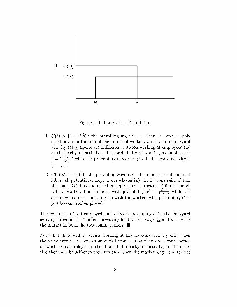
We now turn at the determination of demand and supply of labor.For wage levels greater than �w the labor demand will be zero. For all wagelevel below �w the labor demand will be determined by the number of potentialentrepreneur in the market that is [1 � G(b̂)]: At w = �w the labor demandwill be the interval f0; [1 � G(b̂)]g: The labor supply on the other side willbe 0 for w < w, the interval f0; G(b̂)g at w = w; and will be G(b̂) for w > w:Demand and supply of labor are illustrated in �gure (1).

Lemma 1 There are two possible equilibrium wage rates: either w or �w.

Proof. Not considering the non generic case in which G(b̂) = [1�G(b̂)], wenote that the labor market allows two possible con�gurations:

7

6

-

G(b̂)

w

[1�G(b̂)]

�w

Figure 1: Labor Market Equilibrium

1. G(b̂) > [1 � G(b̂)]; the prevailing wage is w. There is excess supplyof labor and a fraction of the potential workers works at the backyardactivity (at w agents are indi�erent between working as employees andat the backyard activity). The probability of working as employee is

� = (1�G(�))G(�)

while the probability of working in the backyard activity is

(1� �).

2. G(b̂) < [1�G(b̂)]; the prevailing wage is �w. There is excess demand oflabor: all potential entrepreneurs who satisfy the IC constraint obtainthe loan. Of those potential entrepreneurs a fraction G �nd a matchwith a worker; this happens with probability �0 = G(�)

1�G(�)while the

others who do not �nd a match with the worker (with probability (1��0)) become self employed.

The existence of self-employed and of workers employed in the backyardactivity, provides the "bu�er" necessary for the two wages w and �w to clearthe market in both the two con�gurations. �

Note that there will be agents working at the backyard activity only whenthe wage rate is w; (excess supply) because at �w they are always bettero� working as employees rather that at the backyard activity; on the otherside there will be self-entrepreneurs only when the market wage is �w (excess

8

demand) because at w everybody with bt � b̂ can become employer and atthat wage he will be better o� rather than being self employed.Since there are self entrepreneurs only in presence of excess demand of laborand since �w = c, even if ex ante employers and self-entrepreneurs can havedi�erent expected returns, ex post the expected returns are always equal.

3.2 Capital Market Equilibrium

The supply of funds is determined by all agents who are working

Sk(rt) =

Z b̂(rt)

0

bdGt(bt) (8)

while capital demand will be determined by employers and self-entrepreneurs.Because both need the same initial investment the demand of capital is sim-ply:

Dk(rt) =

Z �b

b̂(rt)

(k̂ � b)dGt(bt) (9)

The demand of capital is decreasing in r while the supply is increasing inr. Sk and Dk uniquely determine the equilibrium interest rate. This canbe established noting that given Gt at time t all variables are determinedby the past; for any given level of bt and for any given distribution Gt anincrease in the interest rate, increasing the threshold b̂, increase the supplyand decreases the demand of credit.

4 Market Equilibrium Dynamics

There are four types of individual transition functions corresponding to thefour classes of agents that characterize the economy. Those transition func-tions are represented below:

For those agents with bt < b̂ and work as employees

bt+1 = s[(1 + rt)bt + wt] (10)

For those with bt < b̂ and work at the backyard activity

9

bt+1 = s[(1 + rt)bt + n] (11)

For those with bt > b̂ and become employers

bt+1 =

8<:

shR1k̂ + (1 + rt)bt � (1 + rt)k̂ � wt

iwith probability p

shR0k̂ + (1 + rt)bt � (1 + rt)k̂ � wt

iwith probability (1� p)

(12)

For those with bt > b̂ and become self employed

bt+1 =

8<:

shR

0

1k̂ + (1 + rt)bt � (1 + rt)k̂ � ci

with probability q

shR

0

0k̂ + (1 + rt)bt � (1 + rt)k̂ � ci

with probability (1� q)

(13)

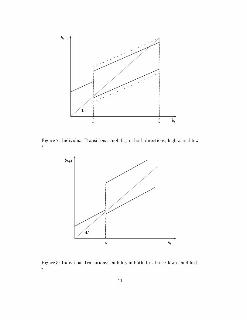
Transition functions like those in equation (10) and (12) are represented in�gures (2) and (3).We place the restriction that s(1 + r) < 1 so that wealth does not growwithout bounds; hence the recurrent distribution is bounded between 0 and~b, where

~b =s

(1� s(1 + r))[R0

1k̂ � (1 + rt)k̂ � wt] (14)

The two bounds mean that nobody can receive a transfer less than zero andthat whoever receives a transfer greater than ~b; even if it becomes a successfulentrepreneur, will leave to his descendants a transfer smaller that the one hehas received. This implies that, even if the support for the initial distributionis the interval [0;�b], in steady state the relevant support for the distributionis [0;~b].

To describe the dynamics of the system we can use the transition functions(10) (12) and �gures (2) and (3). We note however that those transitionfunctions and �gures give only a partial description of the dynamic evolutionof the economy: they are snapshots taken in a given moment of time for agiven distribution of wealth.At the beginning of each period, given the distribution of wealth Gt, bt isgiven, that is it is the result of equilibrium conditions of the previous pe-riod. Once received the bequest bt, agents make their occupational choice;

10

6

-

.................................................bt

.............................................................................

b̂

45Æ

bt+1

~b

Figure 2: Individual Transitions: mobility in both directions; high w and lowr

6

-

.......................................................btb̂

45Æ

bt+1

Figure 3: Individual Transitions: mobility in both directions: low w and highr

11

this choice determines the demand and supply of labor and funds and there-fore determines the distribution of wealth and the equilibrium levels of thewage and the interest rate. Finally, given the equilibrium wage and inter-est rate, each agent bequeath a fraction s of his income to his descendants,determining bt+1.A formal analysis of the dynamics described above is however quite diÆcult.The diÆculties come from two sources:

1. The state space is the set of wealth distributions over [0;�b] and notonly the wealth interval itself.

2. The recursive map on the space of wealth distributions is non linear

In other words wealth follows a non stationary Markov process because theinterest rate and the wage rate a�ect the distribution itself and as the dis-tribution evolves so do w and r. There are very few mathematical resultsthat allow us to deal with Markov processes that are non stationary and weare thus constrained in the dynamical analysis that we can carry out. Inparticular we cannot determine any description of the transitional dynam-ics and we have to restrict the analysis to the steady state. More precisely,following the classi�cation by Owen and Weil (1998) we distinguish betweenconditional and unconditional steady states.

� A conditional steady state is de�ned as a �xed point of the recursivemap that describes the dynamic evolution of the distribution of wealth,holding the wage rate and the interest rate constant.

� An unconditional steady state is a �xed point of that map such thatitself generates the equilibrium wage and interest rate.

4.1 Conditional Steady States

To formally de�ne a conditional steady state, we begin by considering thedynamic process followed by the distribution of wealth, keeping the wage rateand the interest rate �xed. This process can be represented by the followingequation:

Gt+1(b) = H (Gt(b); w; r) (15)

ForG0(b) given. A conditional steady state is a �xed point of the map de�nedin (15).

12

Gcss(b) = H (Gc

ss(b); w; r) (16)

Where the subscript ss denotes steady state values.

The properties of the distribution of wealth that characterize a conditionalsteady state depend on the degree of mobility that there exists betweenclasses. A suÆcient condition for the existence of upward mobility is deter-mined by:

s

1� s(1 + r)�w > b̂ (17)

In the case of high wage and by:

s

1� s(1 + r)w > b̂ (18)

In the case of low wage. That is parents that are working as employees or inthe backyard activity will eventually bequeath to their children an amountof wealth suÆcient to enable them to become entrepreneurs.On the other side a suÆcient condition for downward mobility is determinedby:

s

1� s(1 + r)

hR0

0k̂ � (1 + r)k̂ � �wi< b̂ (19)

In the case of high wage, and by

s

1� s(1 + r)

hR0k̂ � (1 + r)k̂ � w

i< b̂ (20)

In the case of the low wage. That is, after a suÆcient number of bad drawsentrepreneurs (or self employed) will eventually give to their descendants atransfer small enough such that they will not be able to pass the threshold b̂There can be many con�gurations in which there is mobility in both direc-tions, only upwards and only downwards, or no mobility at all.We will skip the analysis of cases in which there is mobility only in onedirection (we will analyze those cases when considering unconditional steadystates) and we will concentrate on the two cases of no-mobility and of mobilityin both directions.

13

In what follows we apply some results recently shown by Hopenhayn andPrescott (1992) (henceforth HP) that rely on the property of monotonicityof Markov processes5.

Lemma 2 Let P be the transition function that describes the Markov processfollowed by wealth. P is monotonically increasing.

Proof. See the Appendix.

Monotonicity alone is enough to ensure the existence of an invariant distri-bution of wealth. This result can be established by applying Corollary 4 byHP that shows the existence of �xed points for monotone maps de�ned overcompact sets; these maps need only to be monotone, and not necessarilylinear. The formal statement of the corollary as of other results obtained byHP is reported in the appendix.

Monotonicity allows us to establish only the existence of a limiting wealthdistribution. In fact there can be many of those distribution; fortunatelyin addition to monotonicity we can establish some other properties of thetransition functions (10) and (12) that allow us to apply Theorem 2 by HPand state the following proposition:

Proposition 1 For any steady state equilibrium pair (rss; wss) the associatedlimiting wealth distribution is unique if there is mobility between classes; thereis a large set of associated limiting wealth distribution if there is no mobilitybetween classes.

Proof. (Follows from Theorem 2 by HP) See the appendix.

Even if the limiting wealth distribution is unique there is nothing that guar-antees that the equilibrium pair (rss; wss) is unique. Most likely there will bemany equilibrium pairs that can sustain a limiting distribution; we will tryto characterize how the di�erent equilibrium con�gurations can look like insection (4.3), for the moment we note that because of the particular con�gu-ration of the labor market we can divide all possible equilibria in two classes:one characterized by low wages and the other by high wages.

5As clear from the �gures, the map from bt to bt+1 is discontinuous; therefore we cannotuse results based on continuity of Markov operators as in Futia (1982).

14

4.2 Unconditional Steady States

So far we have limited the analysis to conditional steady states; we now turnat the analysis of unconditional steady states. They can be de�ned in thefollowing way:i) De�ne H� as the function that maps a pair fw; rg into a conditional steadystate distribution of wealth; that is

H�(fw; rg) = fGcss j G

css = H (Gc

ss; fw; rg)g (21)

ii) Consider now the following function: for any value of G(�) the functionmaps the set of wages and interest rates generated by such a value of G(�)and the set of conditional steady state distribution generated by each pairfw; rg into the set of values of G(�). Call this function �(G). Then

�(G) = (H� (wss; rss)) (22)

An unconditional steady state is a �xed point of

Guss = � (Gu

ss) (23)

The wage rate and the interest rate are uniquely determined by the equilib-rium condition on the labor market and on the market of capital; in case ofboth upward and downward mobility, for any given wage and interest ratethere is a unique conditional steady state distribution of wealth (that is H�(�)is a singleton), however there can be more than one �xed point of (23) asthere can be more that one equilibrium interest rate and wage level. Stillthere is a one to one correspondence between each equilibrium pair frss; wssgand the limiting distribution Gu

ss(b). In case of no-mobility then H� is notanymore unique and the set of limiting distribution will generally be large.

Proposition 2 In case of partial mobilitya) There cannot be an unconditional steady state with only upward mobility.b) There exist an unconditional steady state with only downward mobility.

Proof. Part a) If there is only upward mobility, the number of workerswill progressively decline, and so will the supply of funds. Eventually theresulting interest rate will be so high that the implied threshold will shutdown mobility.

15

Part b) If there is only downward mobility the economy will eventually col-lapse to a "development trap" in which nobody can a�ord to become en-trepreneur and everybody has to work in the backyard activity.�

Proposition 3 For some con�guration of parameters there exist an uncon-ditional steady state in which there is no mobility in any direction.

Proof. See the Appendix.

Proposition 4 Numerical analysis shows that for some con�guration of pa-rameters there exist an unconditional steady state in which there is mobilityin both directions.

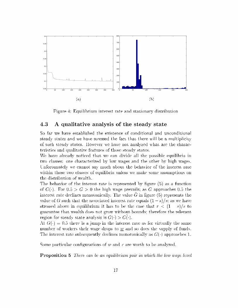
The model was simulated as follows: given the initial distribution and theinitial number of agents total wealth is determined. The total wealth, giventhe project size k̂ determines in turn how many project can be �nanced;sorting the agents by wealth this in turn determines the threshold b̂t. Oncedetermined the threshold, given the other parameter values we can determinethe equilibrium interest rate. The wage, interest and the realization of theproject return determine a new wealth distribution and the process is re-peated until convergence. The simulations assumed 2000 agents distributedaccording to a uniform distribution over the interval [10; 300]6. The modelwas run for 400 periods; the wage rate was set at 100, k̂ was set at 1200;the other parameters were as follows: Rg = 1:3 Rb = 1:2, p = 0:8, � = 0:8,s = 0:67

Figure (4, a) show that with a wage of 100 and the other parameters as de-scribed above the resulting equilibrium interest rate is 9:97% and the impliedthreshold b̂ is 82:6. The associated stationary distribution is represented in�gure (4, b); the values of the parameters and the particular convex technol-ogy give to entrepreneurs a big rent with respect to workers (entrepreneurial(average) income net of wages and interest rate is 208:3, more than the dou-ble of workers' income) this determines a skewed wealth distribution withfew very rich entrepreneurs and many "poor" workers.

6Almost identical results were obtained with a normal distribution.7The saving rate is assumed to take such high values because it denotes saving out of

total wealth and not out of income.

16

0 50 100 150 200 250 300 350 4000.05

0.1

0.15

0.2

0.25

0.3

0.35

0.4

(a)

0 50 100 150 200 2500

100

200

300

400

500

600

700

800

(b)

Figure 4: Equilibrium interest rate and stationary distribution

4.3 A qualitative analysis of the steady state

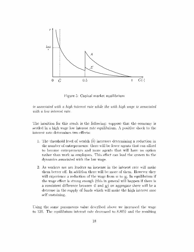
So far we have established the existence of conditional and unconditionalsteady states and we have stressed the fact that there will be a multiplicityof such steady states. However we have not analyzed what are the charac-teristics and qualitative features of those steady states.We have already noticed that we can divide all the possible equilibria intwo classes: one characterized by low wages and the other by high wages.Unfortunately we cannot say much about the behavior of the interest ratewithin those two classes of equilibria unless we make some assumptions onthe distribution of wealth.The behavior of the interest rate is represented by �gure (5) as a functionof G(�). For 0:5 > G > 0 the high wage prevails; as G approaches 0:5 theinterest rate declines monotonically. The value ~G in �gure (5) represents thevalue of G such that the associated interest rate equals (1� s)=s; as we havestressed above in equilibrium it has to be the case that r < (1 � s)=s toguarantee that wealth does not grow without bounds; therefore the relevantregion for steady state analysis is G(�) > ~G(�).At G(�) = 0:5 there is a jump in the interest rate as for virtually the samenumber of workers their wage drops to w and so does the supply of funds.The interest rate subsequently declines monotonically as G(�) approaches 1.

Some particular con�gurations of w and r are worth to be analyzed.

Proposition 5 There can be an equilibrium pair in which the low wage level

17

6

-

r

0:50 1 G(�)

A

A0

.....................................

..........

~G

1�ss

.........

...

...

...

...

...

...

...

..

Figure 5: Capital market equilibrium

is associated with a high interest rate while the with high wage is associatedwith a low interest rate.

The intuition for this result is the following: suppose that the economy issettled in a high wage low interest rate equilibrium. A positive shock to theinterest rate determines two e�ects:

1. The threshold level of wealth (b̂) increases determining a reduction inthe number of entrepreneurs: there will be fewer agents that can a�ordto become entrepreneurs and more agents that will have no optionrather than work as employees. This e�ect can lead the system to thedynamics associated with the low wage.

2. As workers are net lenders an increase in the interest rate will makethem better o�. In addition there will be more of them. However theywill experience a reduction of the wage from �w to w: In equilibrium ifthe wage e�ect is strong enough (this in general will happen if there isa consistent di�erence between �w and w) on aggregate there will be adecrease in the supply of funds which will make the high interest rateself sustaining.

Using the same parameters value described above we increased the wageto 120. The equilibrium interest rate decreased to 8:89% and the resulting

18

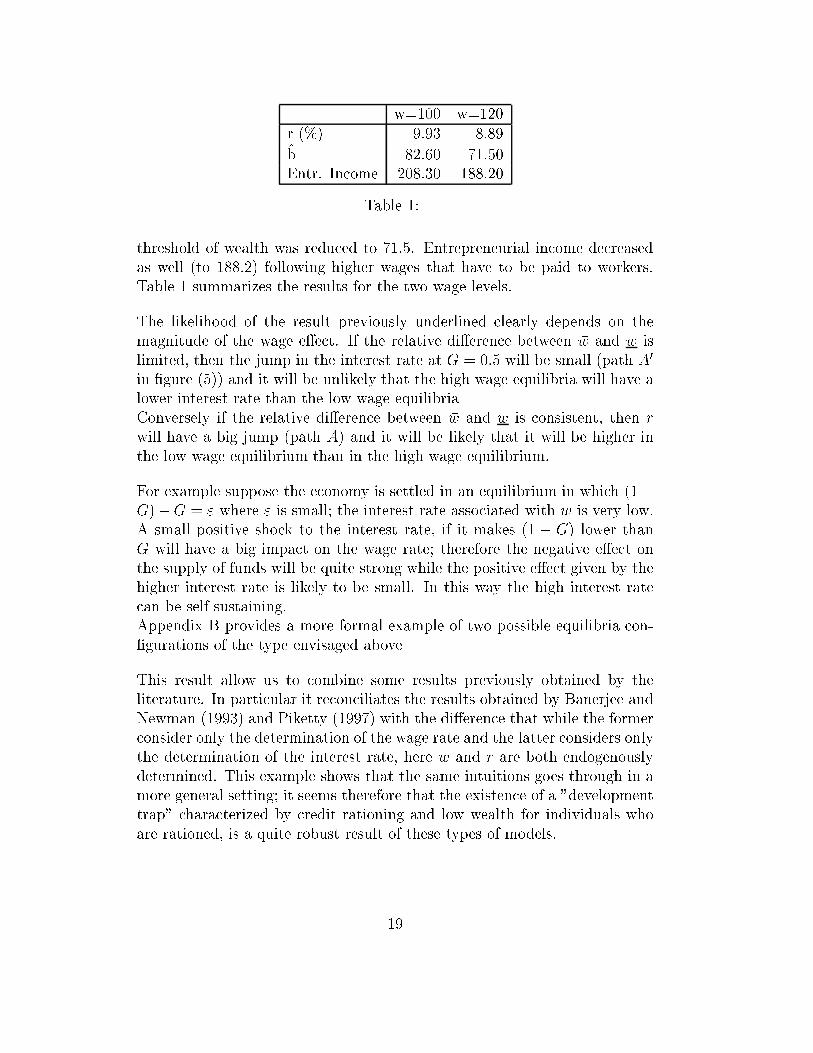
w=100 w=120r (%) 9.93 8.89

b̂ 82.60 71.50Entr. Income 208.30 188.20

Table 1:

threshold of wealth was reduced to 71:5. Entrepreneurial income decreasedas well (to 188:2) following higher wages that have to be paid to workers.Table 1 summarizes the results for the two wage levels.

The likelihood of the result previously underlined clearly depends on themagnitude of the wage e�ect. If the relative di�erence between �w and w islimited, then the jump in the interest rate at G = 0:5 will be small (path A0

in �gure (5)) and it will be unlikely that the high wage equilibria will have alower interest rate than the low wage equilibriaConversely if the relative di�erence between �w and w is consistent, then rwill have a big jump (path A) and it will be likely that it will be higher inthe low wage equilibrium than in the high wage equilibrium.

For example suppose the economy is settled in an equilibrium in which (1�G)�G = " where " is small; the interest rate associated with �w is very low.A small positive shock to the interest rate, if it makes (1 � G) lower thanG will have a big impact on the wage rate; therefore the negative e�ect onthe supply of funds will be quite strong while the positive e�ect given by thehigher interest rate is likely to be small. In this way the high interest ratecan be self sustaining.Appendix B provides a more formal example of two possible equilibria con-�gurations of the type envisaged above

This result allow us to combine some results previously obtained by theliterature. In particular it reconciliates the results obtained by Banerjee andNewman (1993) and Piketty (1997) with the di�erence that while the formerconsider only the determination of the wage rate and the latter considers onlythe determination of the interest rate, here w and r are both endogenouslydetermined. This example shows that the same intuitions goes through in amore general setting; it seems therefore that the existence of a "developmenttrap" characterized by credit rationing and low wealth for individuals whoare rationed, is a quite robust result of these types of models.

19

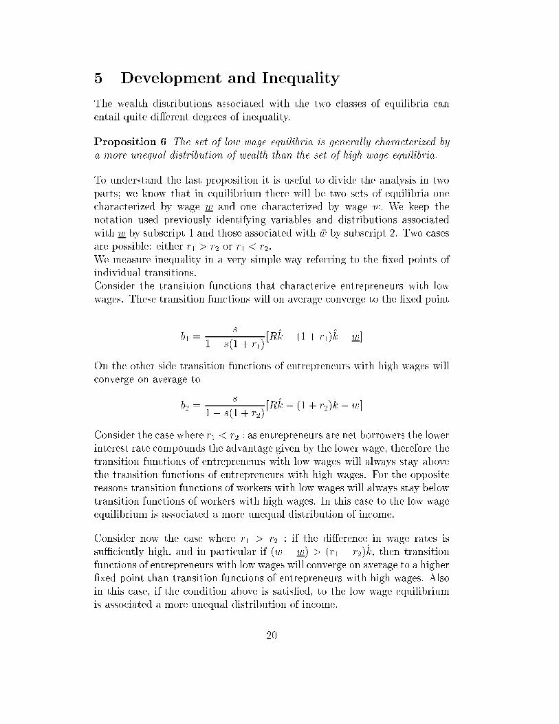
5 Development and Inequality

The wealth distributions associated with the two classes of equilibria canentail quite di�erent degrees of inequality.

Proposition 6 The set of low wage equilibria is generally characterized bya more unequal distribution of wealth than the set of high wage equilibria.

To understand the last proposition it is useful to divide the analysis in twoparts; we know that in equilibrium there will be two sets of equilibria onecharacterized by wage w and one characterized by wage �w: We keep thenotation used previously identifying variables and distributions associatedwith w by subscript 1 and those associated with �w by subscript 2. Two casesare possible: either r1 > r2 or r1 < r2:We measure inequality in a very simple way referring to the �xed points ofindividual transitions.Consider the transition functions that characterize entrepreneurs with lowwages. These transition functions will on average converge to the �xed point

b1 =s

1� s(1 + r1)[ �Rk̂ � (1 + r1)k̂ � w]

On the other side transition functions of entrepreneurs with high wages willconverge on average to

b2 =s

1� s(1 + r2)[ �Rk̂ � (1 + r2)k̂ � �w]

Consider the case where r1 < r2 : as entrepreneurs are net borrowers the lowerinterest rate compounds the advantage given by the lower wage, therefore thetransition functions of entrepreneurs with low wages will always stay abovethe transition functions of entrepreneurs with high wages. For the oppositereasons transition functions of workers with low wages will always stay belowtransition functions of workers with high wages. In this case to the low wageequilibrium is associated a more unequal distribution of income.

Consider now the case where r1 > r2 : if the di�erence in wage rates issuÆciently high, and in particular if ( �w � w) > (r1 � r2)k̂; then transitionfunctions of entrepreneurs with low wages will converge on average to a higher�xed point than transition functions of entrepreneurs with high wages. Alsoin this case, if the condition above is satis�ed, to the low wage equilibriumis associated a more unequal distribution of income.

20

6 Conclusions

In this paper we have characterized the dynamic evolution of an economyin which the distribution of wealth, the equilibrium conditions in the laborand the capital market are endogenously determined in presence of �nancialmarket imperfections.Those imperfections prove to be not only important for the short run devel-opment but they a�ect also the long run evolution of an economy and thedegree of inequality present in steady state.

In our model imperfections in �nancial markets are crucial in giving per-sistence to initial conditions. Without removing those imperfections (forinstance with a clear de�nition of property rights, with a sound regulatoryframework and with fair but severe bankruptcy laws) it will be very diÆ-cult for an economy to get out from a \development trap" in which few richentrepreneurs are getting advantage of low wages paid to workers who arecredit constrained.

Finally this paper makes scope for redistributive policies. Given the factthat there are �nancial market imperfections that can be eased only withdiÆculty, a government may want to engage in redistributive policies thatreduce the degree of inequality. Such one shot policies, in our case, can bewelfare improving having permanent e�ects.

21

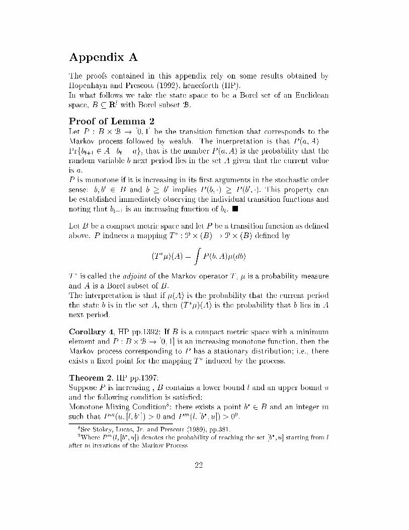
Appendix A

The proofs contained in this appendix rely on some results obtained byHopenhayn and Prescott (1992), henceforth (HP).In what follows we take the state space to be a Borel set of an Euclideanspace, B � Rl with Borel subset B.

Proof of Lemma 2Let P : B � B ! [0; 1] be the transition function that corresponds to theMarkov process followed by wealth. The interpretation is that P (a; A) =Prfbt+1 2 A j bt = ag; that is the number P (a; A) is the probability that therandom variable b next period lies in the set A given that the current valueis a:P is monotone if it is increasing in its �rst arguments in the stochastic ordersense: b; b0 2 B and b � b0 implies P (b; �) � P (b0; �): This property canbe established immediately observing the individual transition functions andnoting that bt+1 is an increasing function of bt. �

Let B be a compact metric space and let P be a transition function as de�nedabove. P induces a mapping T � : P� (B)! P� (B) de�ned by

(T ��)(A) =

ZP (b; A)�(db)

T � is called the adjoint of the Markov operator T , � is a probability measureand A is a Borel subset of B.The interpretation is that if �(A) is the probability that the current periodthe state b is in the set A, then (T ��)(A) is the probability that b lies in Anext period.

Corollary 4, HP pp.1392: If B is a compact metric space with a minimumelement and P : B�B! [0; 1] is an increasing monotone function, then theMarkov process corresponding to P has a stationary distribution; i.e., thereexists a �xed point for the mapping T � induced by the process.

Theorem 2, HP pp.1397:Suppose P is increasing , B contains a lower bound l and an upper bound uand the following condition is satis�ed:Monotone Mixing Condition8: there exists a point b� 2 B and an integer msuch that Pm(u; [l; b�]) > 0 and Pm(l; [b�; u]) > 09:

8See Stokey, Lucas, Jr. and Prescott (1989), pp.381.9Where Pm(l; [b�; u]) denotes the probability of reaching the set [b�; u] starting from l

after m iterations of the Markov Process

22

Then there is a unique stationary distribution �� for the process P and forany initial measure �; T �n� =

RP n(b; �)�(db) converges to ��:

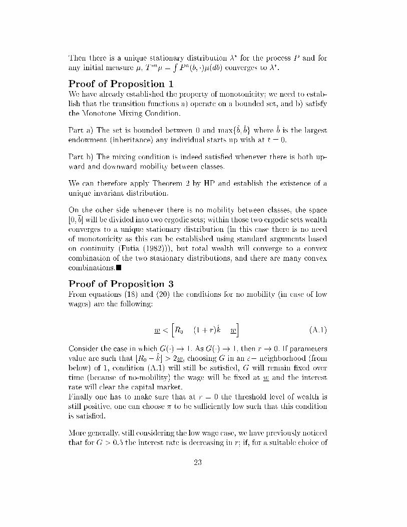
Proof of Proposition 1We have already established the property of monotonicity; we need to estab-lish that the transition functions a) operate on a bounded set, and b) satisfythe Monotone Mixing Condition.

Part a) The set is bounded between 0 and maxf~b;�bg where �b is the largestendowment (inheritance) any individual starts up with at t = 0:

Part b) The mixing condition is indeed satis�ed whenever there is both up-ward and downward mobility between classes.

We can therefore apply Theorem 2 by HP and establish the existence of aunique invariant distribution.

On the other side whenever there is no mobility between classes, the space[0;�b] will be divided into two ergodic sets; within those two ergodic sets wealthconverges to a unique stationary distribution (in this case there is no needof monotonicity as this can be established using standard arguments basedon continuity (Futia (1982))), but total wealth will converge to a convexcombination of the two stationary distributions, and there are many convexcombinations.�

Proof of Proposition 3From equations (18) and (20) the conditions for no mobility (in case of lowwages) are the following:

w <hR0 � (1 + r)k̂ � w

i(A.1)

Consider the case in which G(�)! 1: As G(�)! 1; then r ! 0: If parametersvalue are such that [R0 � k̂] > 2w; choosing G in an "� neighborhood (frombelow) of 1; condition (A.1) will still be satis�ed, G will remain �xed overtime (because of no-mobility) the wage will be �xed at w and the interestrate will clear the capital market.Finally one has to make sure that at r = 0 the threshold level of wealth isstill positive, one can choose � to be suÆciently low such that this conditionis satis�ed.

More generally, still considering the low wage case, we have previously noticedthat for G > 0:5 the interest rate is decreasing in r; if, for a suitable choice of

23

parameters there is a G, let us call it G�, such that equation (A.1) is satis�edwith equality, then for any G� < G < 1 inequality (A.1) will still be satis�edand one can construct an equilibrium like the one above in which there is nomobility between classes. �

24

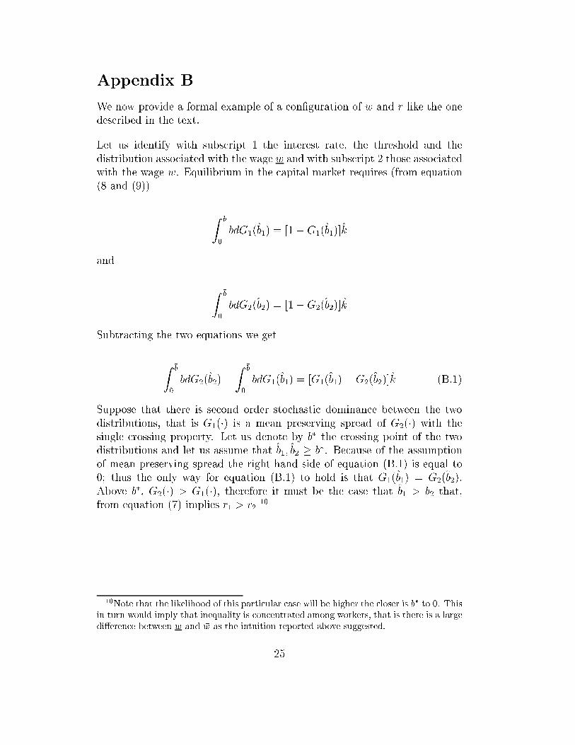
Appendix B

We now provide a formal example of a con�guration of w and r like the onedescribed in the text.

Let us identify with subscript 1 the interest rate, the threshold and thedistribution associated with the wage w and with subscript 2 those associatedwith the wage �w. Equilibrium in the capital market requires (from equation(8 and (9))

Z �b

0

bdG1(b̂1) = [1�G1(b̂1)]k̂

and

Z �b

0

bdG2(b̂2) = [1�G2(b̂2)]k̂

Subtracting the two equations we get

Z �b

0

bdG2(b̂2)�

Z �b

0

bdG1(b̂1) = [G1(b̂1)�G2(b̂2)]k̂ (B.1)

Suppose that there is second order stochastic dominance between the twodistributions, that is G1(�) is a mean preserving spread of G2(�) with thesingle crossing property. Let us denote by b� the crossing point of the twodistributions and let us assume that b̂1; b̂2 � b�. Because of the assumptionof mean preserving spread the right hand side of equation (B.1) is equal to0; thus the only way for equation (B.1) to hold is that G1(b̂1) = G2(b̂2).Above b�, G2(�) > G1(�), therefore it must be the case that b̂1 > b̂2 that,from equation (7) implies r1 > r2

10

10Note that the likelihood of this particular case will be higher the closer is b� to 0. Thisin turn would imply that inequality is concentrated among workers, that is there is a largedi�erence between w and �w as the intuition reported above suggested.

25

References

Aghion, Philippe and Patrick Bolton, \A Theory of Trickle-DownGrowth and Development with Debt-Overhang," Review of EconomicStudies, 1997, 64, 151{172.

Banerjee, Abhijit and Andrew F. Newman, \Occupational Choice andthe Process of Development," Journal of Political Economy, 1993, 101,274{298.

and , \Poverty, Incentives, and Development," American Eco-nomic Review Papers and Proceedings, 1994, 84, 211{215.

and , \Information, the Dual Economy, and Development," Re-view of Economic Studies, 1998, 65 (4), 631{654.

Bhattacharya, Jodeep, \Credit Market Imperfections, Income Distribu-tion and Capital Accumulation," Economic Theory, 1998, 11 (1), 171{200.

Futia, Carl A., \Invariant Distributions and the Limiting Behavior ofMarkovian Economic Models," Econometrica, 1982, 50 (2), 377{408.

Galor, Oded and Joseph Zeira, \Income Distribution and Macroeco-nomics," Review of Economic Studies, 1993, 60, 35{52.

Hopenhayn, Hugo A. and Edward C. Prescott, \Stochastic Mono-tonicity and Stationary Distributions for Dynamic Economies," Econo-metrica, 1992, 60 (6), 1387{1406.

Lucas, Robert E., \On the Mechanics of Economic Development," Journalof Monetary Economics, 1988, 22, 3{42.

Murphy, Kevin M., Andrei Shleifer, and Robert W. Vishny, \In-dustrialization and the Big Push," Journal of Political Economy, 1989,97, 1003{1026.

Owen, Ann L. and David N. Weil, \Intergenerational Earnings Mobility,Inequality and Growth," Journal of Monetary Economics, 1998, 41, 71{104.

Piketty, Thomas, \The Dynamics of the Wealth Distribution and the In-terest Rate with Credit Rationing," Review of Economic Studies, 1997,64, 173{189.

26

Romer, Paul, \Increasing Returns and Long Run Growth," Journal ofPolitical Economy, 1986, 94, 1002{1037.

Stokey, Nancy, Robert E. Lucas, Jr., and Edward C. Prescott,Recursive Methods in Economic Dynamics, Harvard University Press,1989.

World Bank, Word Development Report: Financial Systems and Develop-ment, Oxford University Press, 1989.

, World Development Report: From Plan to Market, Oxford UniversityPress, 1996.

27