DEPARTMENT OF ECONOMICS AND FINANCE

SCHOOL OF BUSINESS AND ECONOMICS

UNIVERSITY OF CANTERBURY

CHRISTCHURCH, NEW ZEALAND

Taxes and Economic Growth in OECD Countries: A Meta-Analysis

Nazila Alinaghi W. Robert Reed

WORKING PAPER

No. 37/2016

Department of Economics and Finance School of Business and Economics

University of Canterbury Private Bag 4800, Christchurch

New Zealand

WORKING PAPER No. 37/2016

Taxes and Economic Growth in OECD Countries: A Meta-Analysis

Nazila Alinaghi1

W. Robert Reed1†

15 December 2016

Abstract: This paper uses meta-analysis to evaluate the results of 42 studies and 641 individual estimates of the effect of taxes on economic growth in OECD countries. Our analysis addresses a number of difficult coding issues such as: implications of the government budget constraint for interpretations of tax effects; units of measurement for economic growth rates and tax rates; implications of equation specifications that measure short-run, medium-run, and long-run effects; length of time period (annual data versus multi-year periods); and other factors. Our main findings are: Estimates in the literature are characterized by significant (negative) publication bias. Controlling for publication bias, we find that increases in unproductive expenditures funded by distortionary taxes and/or deficits have a significant, negative effect on growth; while increases in non-distortionary taxes to fund productive expenditures and/or government surpluses have a significant, positive effect. The estimated differences in these policies indicate that there is scope for tax policy to have a meaningful impact on economic growth. Finally, we find weak evidence that taxes on labour are more growth retarding than other types of taxes, while the evidence regarding other types of taxes is mixed. Keywords: Meta-analysis, taxes, economic growth, OECD JEL Classifications: H2, H5, H6, O47, O50 Acknowledgments. We are grateful for helpful comments received from Norman Gemmell; Chris Heady; Joe Stone; and participants at the Meta-Analysis of Economics Research Network (MAER-Net) Colloquium, 15-17 September, 2016, Hendrix College, Conway, Arkansas, USA, and the Applied Econometrics Workshop, 28 October, 2016, Victoria University, Wellington, NEW ZEALAND. 1 Department of Economics and Finance, University of Canterbury, Christchurch, NEW ZEALAND

* Corresponding author is W. Robert Reed. His email address is bob.reed@canterbury.ac.nz.

1

I. INTRODUCTION This study is a meta-analysis of the effect of taxes on economic growth in OECD countries.

Over the decades, there have been hundreds of studies estimating the effect of taxes on

economic growth. Prominent examples include Agell, Lindh, and Ohlsson (1997); Mendoza,

Milesi-Ferretti, and Asea (1997); Fölster and Henrekson (1999); Kneller, Bleaney, and

Gemmell (1999); Daveri and Tabellini (2000); Bassanini and Hemmings (2001); Bleaney,

Gemmell, and Kneller (2001); Fölster and Henrekson (2001); Afonso and Furceri (2010);

Alesina and Ardagna (2010); and Arnold et al. (2011). Despite the fact that many studies use

similar data and study many of the same countries and time periods, estimates vary widely, so

that there is no consensus on whether taxes exert an important influence on economic growth

and, if they do, how large an effect they have.

There are many possible reasons for this state of affairs. Tax policy is necessarily a two-

sided activity. Revenues generated through taxes are used to fund expenditures and/or reduce

deficits. As a result, tax effects are always net effects, and will differ depending on how the tax

revenues are spent. Relatedly, different types of taxes may have different consequences for

economic growth, as may different types of expenditures (Barro, 1990; Barro and Sala-i-

Martin, 1992; Futagami et al., 1993; and Deverajan et al., 1996). For example, a distortionary

tax on corporate profits used to fund transfer payments may be expected to have different

growth effects than a non-distortionary tax on goods and services used to build productive

infrastructure. Further, the empirical models used to estimate tax effects may measure short-

run, medium-run, or long-run effects depending on the particular ways that regression

equations are specified. For these and other reasons, even studies that use similar data can

produce dissimilar estimates of tax effects.

In order to make estimates comparable across studies, one must carefully track the

factors that can cause tax effects to differ. Once this is done, standard meta-analysis procedures

2

can be used to control for these factors. This allows one to aggregate and compare estimates

across studies. That is what this analysis does.

This research has three goals. First, we wish to summarize the extensive literature on

taxes and economic growth in OECD countries. As part of this analysis, we check for

publication bias, by which some estimates are disproportionately reported, either due to

statistical insignificance, or because they are “wrong-signed” (Stanley and Doucouliagos,

2012; Havranek and Irsova, 2012). We then calculate an “overall tax effect” that corrects for

publication bias.

Unfortunately, any measure of the “overall effect” of taxes on growth is not particularly

informative because it lumps together estimated effects from different kinds of fiscal policies.

Accordingly, our second goal is to compare estimated tax effects from two types of policies.

On the one hand, we group tax effects that are predicted to have a negative impact on economic

growth. An example would be the use of distortionary taxes to fund unproductive expenditures.

On the other hand are tax effects that are predicted to positively impact economic growth, such

as the use of non-distortionary taxes to fund productive expenditures. The difference in these

two sets of estimated tax effects provides a measure of the impact that tax policy can have on

economic growth. Our third goal and final goal is to determine whether some kinds of taxes

are more growth-retarding than others.

To achieve these goals, this study collects estimates of tax effects on economic growth

in OECD countries from 42 studies. Based on a final sample of 641 estimates, we find strong

evidence that the empirical literature on estimated tax effects is impacted by publication bias.

In particular, there is a tendency to over-report negative estimates. Once we control for this,

we calculate that the “overall effect” of taxes on economic growth is small and statistically

insignificant. However, as noted above, this “overall tax effect” is not very informative.

3

When we turn to analysing different types of tax policies, and after controlling for

publication bias, we find evidence that the composition of fiscal policy makes a difference. For

example, increases in unproductive expenditures funded by distortionary taxes and/or deficits

have a statistically significant, negative effect on economic growth. Increases in non-

distortionary taxes to fund productive expenditures and/or government surpluses have a

statistically significant, positive effect on economic growth. The estimated differences in these

policies indicate that there is scope for tax policy to have a meaningful impact on economic

growth. Further, we find weak evidence that taxes on labour are more growth-retarding than

other types of taxes. Evidence regarding other types of taxes is mixed.

Our analysis proceeds as follows. Section II reports how we collected our sample of

estimates. Section III discusses some of the reasons why studies of tax effects can produce

different estimates. Section IV presents our empirical results, addressing each of the three goals

above. Section V summarizes the main findings of our research.

II. SELECTION OF STUDIES AND CONSTRUCTION OF DATASET This meta-analysis collects estimated tax effects for all studies that estimate a variation of the

following specification:

(1) 𝑔𝑔 = 𝛼𝛼0 + 𝛼𝛼1𝑡𝑡𝑡𝑡 + 𝑒𝑒𝑡𝑡𝑡𝑡𝑒𝑒𝑡𝑡,

where 𝑔𝑔 is a measure of economic growth, 𝑡𝑡𝑡𝑡 is a measure of the tax rate, and the data are taken

from OECD countries.1 To do that, we conducted a comprehensive search including both

electronic and manual search procedures.

The electronic search used three categories of keywords: (i) “TAX” keywords, (ii)

“ECONOMIC GROWTH” keywords, and (iii) “OECD” keywords in the following

combination: “TAX” and “ECONOMIC GROWTH” and “OECD”. A variety of keywords

1 We did not include studies that estimate nonlinear tax effects, such as the “growth hills” of Bania, Gray and Stone (2007).

4

were substituted for each of the three categories. These are reported in APPENDIX 1. Keyword

combinations were searched using the following search engines: EconLit, Google Scholar,

JSTOR, Web of Science, Scopus, RePEc, EBSCO, and ProQuest. A total of 303 studies were

identified in this manner.

The abstracts and conclusions of these studies were then read to eliminate any studies

that did not estimate a growth equation with a tax variable, and/or included countries other than

OECD countries. Backwards and forwards citation searches were used to locate additional

studies. This produced a list of 51 studies, some of which were multiple versions of the same

study2, and included journal articles, conference proceedings, studies from think tanks and

research firms, theses and dissertations, and working papers and other unpublished research.

This list was emailed to 64 researchers who had published on the topic of taxes and

economic growth. The researchers were asked for help in identifying additional research,

including working papers or unpublished studies from PhD students. Based on their responses,

a revised list of 54 studies was compiled.

The new list was then read carefully to identify eligible studies. The dependent variable

had to be a measure of GDP growth.3 The growth equation had to include a tax variable that

was measured in units of percent of income.4 The countries included in a given regression

equation had to consist entirely of OECD countries, though they could be restricted to a subset

of OECD countries such as the G7, EU-15 or a larger set of EU member nations. Further, all

estimates had to include multiple countries; i.e., we eliminated single country studies.5 All

estimated tax effects had to report a standard error or associated t-statistic. Finally, only studies

2 When multiple versions of the same paper included different estimates, we pooled the estimates across versions. 3 Alternatively, the dependent variable could be the level of income, as long as the explanatory variables included its lag. 4 Studies where the “tax variable” consisted of all revenues, such as the ratio of total revenues to GDP, were not included. 5 Time series from individual countries pose problems because relatively short data ranges combined with a relatively large number of confounders leaves few degrees of freedom. As a result, we chose not to include individual country studies in our meta-analysis.

5

written in English were included. We closed our search on 13 January 2016. The final sample

of 42 studies is listed in APPENDIX 2.

Once the final set of estimates was determined, we then went through each

equation/estimate and coded a set of regression and study characteristics (see next section).

The coding was done independently by at least two coders, including both authors of this study,

with a careful reconciliation of any discrepancies or inconsistencies. All search and coding

procedures followed the MAER-NET protocols (Stanley et al., 2013).

III. FACTORS THAT CAUSE TAX ESTIMATES TO DIFFER ACROSS STUDIES The government budget constraint. There are a number of issues that must be addressed before

one can obtain meaningful estimates of tax effects. The first has to do with the government

budget constraint:

(2) 0 = 𝑇𝑇𝑇𝑇𝑇𝑇𝑒𝑒𝑇𝑇 + 𝑂𝑂𝑡𝑡ℎ𝑒𝑒𝑡𝑡𝑒𝑒𝑒𝑒𝑒𝑒𝑒𝑒𝑒𝑒𝑒𝑒𝑒𝑒𝑇𝑇 − 𝐸𝐸𝑇𝑇𝐸𝐸𝑒𝑒𝑒𝑒𝐸𝐸𝐸𝐸𝑡𝑡𝑒𝑒𝑡𝑡𝑒𝑒𝑇𝑇 − 𝑆𝑆𝑒𝑒𝑡𝑡𝐸𝐸𝑆𝑆𝑒𝑒𝑇𝑇.

This can be rewritten as:

(3) 0 = 𝑡𝑡𝑡𝑡 + �𝑂𝑂𝑂𝑂ℎ𝑒𝑒𝑒𝑒𝑒𝑒𝑒𝑒𝑒𝑒𝑒𝑒𝑒𝑒𝑒𝑒𝑒𝑒𝑒𝑒𝐼𝐼𝑒𝑒𝐼𝐼𝐼𝐼𝐼𝐼𝑒𝑒

� − �𝐸𝐸𝐸𝐸𝐸𝐸𝑒𝑒𝑒𝑒𝐸𝐸𝐸𝐸𝑂𝑂𝑒𝑒𝑒𝑒𝑒𝑒𝑒𝑒𝐼𝐼𝑒𝑒𝐼𝐼𝐼𝐼𝐼𝐼𝑒𝑒

� − �𝑆𝑆𝑒𝑒𝑒𝑒𝐸𝐸𝑆𝑆𝑒𝑒𝑒𝑒𝐼𝐼𝑒𝑒𝐼𝐼𝐼𝐼𝐼𝐼𝑒𝑒

�,

where for the moment we define the tax rate as the ratio of taxes over income, 𝑡𝑡𝑡𝑡 = � 𝑇𝑇𝑇𝑇𝐸𝐸𝑒𝑒𝑒𝑒𝐼𝐼𝑒𝑒𝐼𝐼𝐼𝐼𝐼𝐼𝑒𝑒

�.

In estimating Equation (1), it should be apparent that the interpretation of 𝛼𝛼1 will differ

depending on which variable(s) are omitted from Equation (3). If �𝐸𝐸𝐸𝐸𝐸𝐸𝑒𝑒𝑒𝑒𝐸𝐸𝐸𝐸𝑂𝑂𝑒𝑒𝑒𝑒𝑒𝑒𝑒𝑒𝐼𝐼𝑒𝑒𝐼𝐼𝐼𝐼𝐼𝐼𝑒𝑒

� is omitted,

then 𝛼𝛼1 measures the net effect of an increase in expenditures funded by taxes. Alternatively,

if �𝑆𝑆𝑒𝑒𝑒𝑒𝐸𝐸𝑆𝑆𝑒𝑒𝑒𝑒𝐼𝐼𝑒𝑒𝐼𝐼𝐼𝐼𝐼𝐼𝑒𝑒

� is omitted and expenditures are held constant, then 𝛼𝛼1 measures the net effect of

an increase in taxes used to cut the deficit (or increase the surplus).

Things become more complicated when finer gradations of taxes and expenditures are

used. For example, empirical analyses of fiscal policy sometimes divide taxes into (i)

6

distortionary and (ii) non-distortionary taxes; and expenditures into (i) productive and (ii)

unproductive expenditures.

(4) 0 = 𝑡𝑡𝑡𝑡(𝑁𝑁𝑒𝑒𝑒𝑒 − 𝐸𝐸𝐸𝐸𝑇𝑇𝑡𝑡𝑒𝑒𝑡𝑡𝑡𝑡𝐸𝐸𝑒𝑒𝑒𝑒𝑇𝑇𝑡𝑡𝑑𝑑) + 𝑡𝑡𝑡𝑡(𝐷𝐷𝐸𝐸𝑇𝑇𝑡𝑡𝑒𝑒𝑡𝑡𝑡𝑡𝐸𝐸𝑒𝑒𝑒𝑒𝑇𝑇𝑡𝑡𝑑𝑑) + �𝑂𝑂𝑂𝑂ℎ𝑒𝑒𝑒𝑒𝑒𝑒𝑒𝑒𝑒𝑒𝑒𝑒𝑒𝑒𝑒𝑒𝑒𝑒𝑒𝑒𝐼𝐼𝑒𝑒𝐼𝐼𝐼𝐼𝐼𝐼𝑒𝑒

�

−�𝑃𝑃𝑡𝑡𝑒𝑒𝐸𝐸𝑒𝑒𝑃𝑃𝑡𝑡𝐸𝐸𝑒𝑒𝑒𝑒 𝐸𝐸𝑇𝑇𝐸𝐸𝑒𝑒𝑒𝑒𝐸𝐸𝐸𝐸𝑡𝑡𝑒𝑒𝑡𝑡𝑒𝑒𝑇𝑇

𝐼𝐼𝑒𝑒𝑃𝑃𝑒𝑒𝐼𝐼𝑒𝑒� − �

𝑈𝑈𝑒𝑒𝐸𝐸𝑡𝑡𝑒𝑒𝐸𝐸𝑒𝑒𝑃𝑃𝑡𝑡𝐸𝐸𝑒𝑒𝑒𝑒 𝐸𝐸𝑇𝑇𝐸𝐸𝑒𝑒𝑒𝑒𝐸𝐸𝐸𝐸𝑡𝑡𝑒𝑒𝑡𝑡𝑒𝑒𝑇𝑇𝐼𝐼𝑒𝑒𝑃𝑃𝑒𝑒𝐼𝐼𝑒𝑒

�

−�𝑆𝑆𝑒𝑒𝑒𝑒𝐸𝐸𝑆𝑆𝑒𝑒𝑒𝑒𝐼𝐼𝑒𝑒𝐼𝐼𝐼𝐼𝐼𝐼𝑒𝑒

�.

If �𝑃𝑃𝑒𝑒𝐼𝐼𝐸𝐸𝑒𝑒𝐼𝐼𝑂𝑂𝐸𝐸𝑒𝑒𝑒𝑒 𝐸𝐸𝐸𝐸𝐸𝐸𝑒𝑒𝑒𝑒𝐸𝐸𝐸𝐸𝑂𝑂𝑒𝑒𝑒𝑒𝑒𝑒𝑒𝑒𝐼𝐼𝑒𝑒𝐼𝐼𝐼𝐼𝐼𝐼𝑒𝑒

� is omitted, the coefficient on the non-distortionary tax

rate variable measures the net effect of an increase in productive expenditures funded by an

increase in non-distortionary taxes. As discussed below, it is generally accepted that growth

theory predicts a positive value for 𝛼𝛼1 in this case. In contrast, if

�𝑈𝑈𝑒𝑒𝐸𝐸𝑒𝑒𝐼𝐼𝐸𝐸𝑒𝑒𝐼𝐼𝑂𝑂𝐸𝐸𝑒𝑒𝑒𝑒 𝐸𝐸𝐸𝐸𝐸𝐸𝑒𝑒𝑒𝑒𝐸𝐸𝐸𝐸𝑂𝑂𝑒𝑒𝑒𝑒𝑒𝑒𝑒𝑒𝐼𝐼𝑒𝑒𝐼𝐼𝐼𝐼𝐼𝐼𝑒𝑒

� is omitted, the coefficient on the distortionary tax rate variable

measures the net effect of an increase in unproductive expenditures funded by an increase in

distortionary taxes. In this case, a negative value for 𝛼𝛼1 would be expected. As a result, the two

“tax rate” variables might legitimately produce opposite signs by virtue of the kind of tax

variable that was being investigated, and depending on which other variables in the government

budget constraint were omitted.

To address this issue, we go through each estimated tax effect and identify both the

operative tax types and the use of the tax revenues implied by the government budget

constraint. Tax types and expenditures are then categorized as distortionary/non-distortionary,

productive/unproductive, or other according to the taxonomy in TABLE 1, taken from Kneller,

Bleaney, and Gemmell (1999).6 We then use TABLE 2, which is taken from Gemmell, Kneller,

and Sanz (2009) and summarizes predictions from growth theory, to predict the effect on

6 We use the Kneller, Bleaney, and Gemmell (1999) taxonomy because it is broadly representative of the fiscal policy literature. It may be best thought of as representing relative categories. Strictly speaking, any tax that is not lump-sum is distortionary.

7

growth for the associated fiscal policy actions. In this way, every tax effect is assigned a

prediction with respect to its impact on growth (negative, positive, or ambiguous).

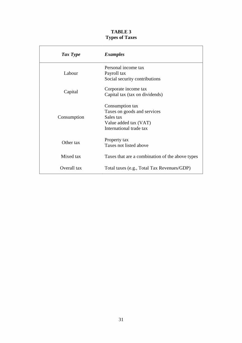
We also classify each estimated tax effect according to its tax type. Taxes are classified

as Labour taxes, Capital taxes, Consumption taxes, Mixed taxes, Other taxes, and Overall taxes.

The classification system for assigning each tax to a tax type is given in TABLE 3.

Units of measurement. The second issue has to do with the units of measurement for

the 𝑔𝑔 and 𝑡𝑡𝑡𝑡 variables. Each of these variables can be measured in percentage points (e.g., 2%)

or in decimals (0.02). This will obviously effect the size of the tax coefficient, 𝛼𝛼1. For example,

if a one-percentage point increase in the tax rate lowers growth by 0.1%, and if both 𝑔𝑔 and 𝑡𝑡𝑡𝑡

are measured in percentage points, or both are measured in decimals, then the corresponding

value of 𝛼𝛼1 will be -0.1. However, if 𝑔𝑔 is measured in percentage points, and 𝑡𝑡𝑡𝑡 is measured in

decimals, then the corresponding value of 𝛼𝛼1 will be -10. And if 𝑔𝑔 is measured in decimals,

and 𝑡𝑡𝑡𝑡 is measured in percentage points, then the value of 𝛼𝛼1 will be -0.001. Accordingly, we

adjust all estimated effects so that 𝛼𝛼1 = 𝑋𝑋 means that a one-percentage point increase in the

tax rate is associated with an X percentage point increase in economic growth.7

Countries. The third issue relates to the specific countries included in a given study.

There is a trade-off between including a large number of countries, and including countries that

are relatively homogeneous. We focus on studies that limit their estimation to OECD countries.

APPENDIX 3 lists the 34 countries of the OECD, ordered by their year of admission to the

OECD8. Many studies only include a subset of these countries. We further categorize the

countries by the groupings G-7, EU-15, and EU, with the idea that the smaller groupings consist

of more homogeneous economies. Our meta-analysis controls for these different groupings to

7 Sometimes it was difficult to determine the units of measurement of the respective variables from the study so as to properly interpret the coefficient. When this would happen, we would contact the original author(s). When there was substantial uncertainty about the interpretation of the coefficient, the estimate was dropped from our analysis. 8 Latvia, the 35th member, was admitted to the OECD on July 1st, 2016.

8

identify whether the estimated tax effects vary systematically across the different sets of

countries included in the original studies.

Duration of time periods. A fourth issue concerns the time frames of the data employed

by the different studies. If the time periods of Equation (1) differ across studies, that could

cause estimates of 𝛼𝛼1 to differ, even when the underlying effect is the same. For example,

suppose there were two growth studies, one used 5-year time periods, the other used annual

data. Suppose the former measured the cumulative rate of growth over each five-year period,

while the latter reported annual growth rates. All things constant, one might expect 𝛼𝛼1 to be

larger in the former case. Accordingly, we adjust all growth measures to be (average) annual

rates of growth.

Duration of estimated tax effects. A fifth issue is related in that it has to do with the

duration of the estimated tax effect as implied by the specification of the regression equation.

Let the estimated relationship between growth, 𝑔𝑔, and the tax rate variable, tr, be given by the

finite distributed lag model,

(5) 𝑔𝑔𝑂𝑂 = 𝛼𝛼0 + 𝛼𝛼1𝑡𝑡𝑡𝑡𝑂𝑂 + 𝛼𝛼2𝑡𝑡𝑡𝑡𝑂𝑂−1 + 𝜀𝜀𝑂𝑂.

If this is the model estimated by the original study, then 𝛼𝛼1 and 𝛼𝛼2 represent the “short-

run/immediate” effects of a one-percentage point increase in taxes in years t and t-1 on

economic growth in year t.

By adding and subtracting 𝛼𝛼2𝑡𝑡𝑡𝑡𝑂𝑂 to the right hand side, one can rewrite the above as:

(6) 𝑔𝑔𝑂𝑂 = 𝛼𝛼0 + 𝜏𝜏 𝑡𝑡𝑡𝑡𝑂𝑂 − 𝛼𝛼2∆𝑡𝑡𝑡𝑡𝑂𝑂 + 𝜀𝜀𝑂𝑂,

where 𝜏𝜏 = (𝛼𝛼1 + 𝛼𝛼2). If this is the model estimated in the original study, then the coefficient

on the current tax rate, 𝜏𝜏, represents the “cumulative/intermediate” effect of a one-percentage

point increase in taxes in year t and t-1 on economic growth in year t.

An alternative specification to Equation (5) is the auto-regressive, distributed lag

model,

9

(7) 𝑔𝑔𝑂𝑂 = 𝛼𝛼0 + 𝛼𝛼1𝑡𝑡𝑡𝑡𝑂𝑂 + 𝛼𝛼2𝑡𝑡𝑡𝑡𝑂𝑂−1 + 𝛾𝛾𝑔𝑔𝑂𝑂−1 + 𝜀𝜀𝑂𝑂.

Subtracting 𝑔𝑔𝑂𝑂−1 from both sides gives:

(8) ∆𝑔𝑔𝑂𝑂 = 𝛼𝛼0 + 𝛼𝛼1𝑡𝑡𝑡𝑡𝑂𝑂 + 𝛼𝛼2𝑡𝑡𝑡𝑡𝑂𝑂−1 + (𝛾𝛾 − 1)𝑔𝑔𝑂𝑂−1 + 𝜀𝜀𝑂𝑂,

which can be rewritten in error correction form as:

(9) ∆𝑔𝑔𝑂𝑂 = 𝛼𝛼0 + 𝛿𝛿(𝑔𝑔𝑂𝑂−1 − 𝜃𝜃𝑡𝑡𝑡𝑡𝑂𝑂) − 𝛼𝛼2∆𝑡𝑡𝑡𝑡𝑂𝑂 + 𝜀𝜀𝑂𝑂 ,

where 𝛿𝛿 = (𝛾𝛾 − 1) and 𝜃𝜃 = (𝛼𝛼1+𝛼𝛼2)(1−𝛾𝛾) . This specification is common in recent mean group and

pooled mean group studies of economic growth. In Equation (9), the coefficient on 𝑡𝑡𝑡𝑡𝑂𝑂 in the

cointegrating equation, 𝜃𝜃, represents the total, long-run effect of a permanent, one-percentage

point increase in the tax rate on steady-state economic growth.9

Specifications (5), (6), and (9) lead to three different measures of the effect of taxes on

economic growth. Our meta-analysis controls for this by noting the specification of the growth

equation in the original study and categorizing the duration of the estimated tax effect as short-

run, medium-run, or long-run.

Different measures for economic growth and tax rates. A final issue that directly relates

to the coding of tax effects has to do with how the economic growth and tax rate variables are

defined. Some studies measure economic growth in terms of nominal GDP, some in terms of

real GDP. Some measure economic growth in terms of per capita GDP, and some total GDP.10

When it comes to measuring “the tax rate,” most studies use effective tax rates, defined as tax

revenues over a given measure of income. Others use statutory tax rates -- typically the top

marginal rate. And some studies attempt to distinguish marginal from average tax rates. We

use dummy variables to indicate the specific measures underlying a given estimate.

9 We note that Equation (9) is sometimes estimated using an equivalent, alternative specification: ∆𝑔𝑔𝑂𝑂 = 𝛼𝛼0 + 𝛿𝛿(𝑔𝑔𝑂𝑂−1 − 𝜃𝜃𝑡𝑡𝑡𝑡𝑂𝑂−1) + 𝛼𝛼1∆𝑡𝑡𝑡𝑡𝑂𝑂 + 𝜀𝜀𝑂𝑂 , where 𝛿𝛿 and 𝜃𝜃 are defined as above. 10 We do not distinguish between real and nominal growth because studies that used (the log of) nominal GDP also included time dummies, so that there was no effective difference between specifying economic growth in nominal or real terms.

10

Control variables. In addition to the issues identified above, our analysis codes for many

other study characteristics, including estimation method; type of standard error; whether the

original study was published in a peer-reviewed journal; year of publication; length of sample

period; midyear of sample period; inclusion of specific variables such as country fixed effects,

human capital, trade openness, inflation, and others. A full list of the variables used in this

study is discussed below.

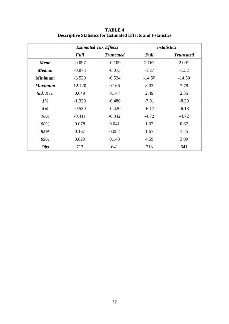
IV. EMPIRICAL ANALYSIS Preliminary analysis. Our literature search produced a dataset consisting of 713 estimated tax

effects. TABLE 4 reports descriptive statistics for both these estimates and the associated t-

statistics. For the full dataset, the median estimated tax effect is -0.073, implying that a ten

percentage point increase in the tax rate is associated with a 0.73 percentage point decrease in

annual economic growth. This compares to an average, annual growth rate for OECD countries

of approximately 2.5 per cent over the period 1970-2000, a period which roughly corresponds

to the “average” sample period of the studies included in this meta-analysis.11,12 The median t-

statistic is -1.27.

TABLE 4 immediately identifies a problem in that the minimum and maximum

estimated tax effects are -3.52 and 12.72. These values indicate a tax effect size that is

considerably outside the bounds of reasonable. While researchers differ in their estimates of

the effects of taxes, nobody suggests that a one percentage point increase in the tax rate would

lower annual economic growth by over 3 percentage points, or increase it by over 12 percentage

points. Accordingly, the subsequent analysis works with a truncated sample of estimates.

We delete the top and bottom 5 percent of estimates and obtain a sample of 641

estimated tax effects. The descriptive statistics for this truncated sample is also reported in

11 This is calculated by taking the average beginning and average ending dates for the sample ranges of the respective studies. 12 Growth rate is the average, annual growth rate over the period 1970-2000 for the 22 countries that belonged to the OECD in 1970.

11

TABLE 4. The range of estimated tax effects for this sample range from a minimum of -0.524

to a maximum of 0.166. The median t-statistic still indicates insignificance, while the sample

of t-statistics range from a minimum of -14.50 to a maximum of 7.78, with a mean absolute

value of 2.09.

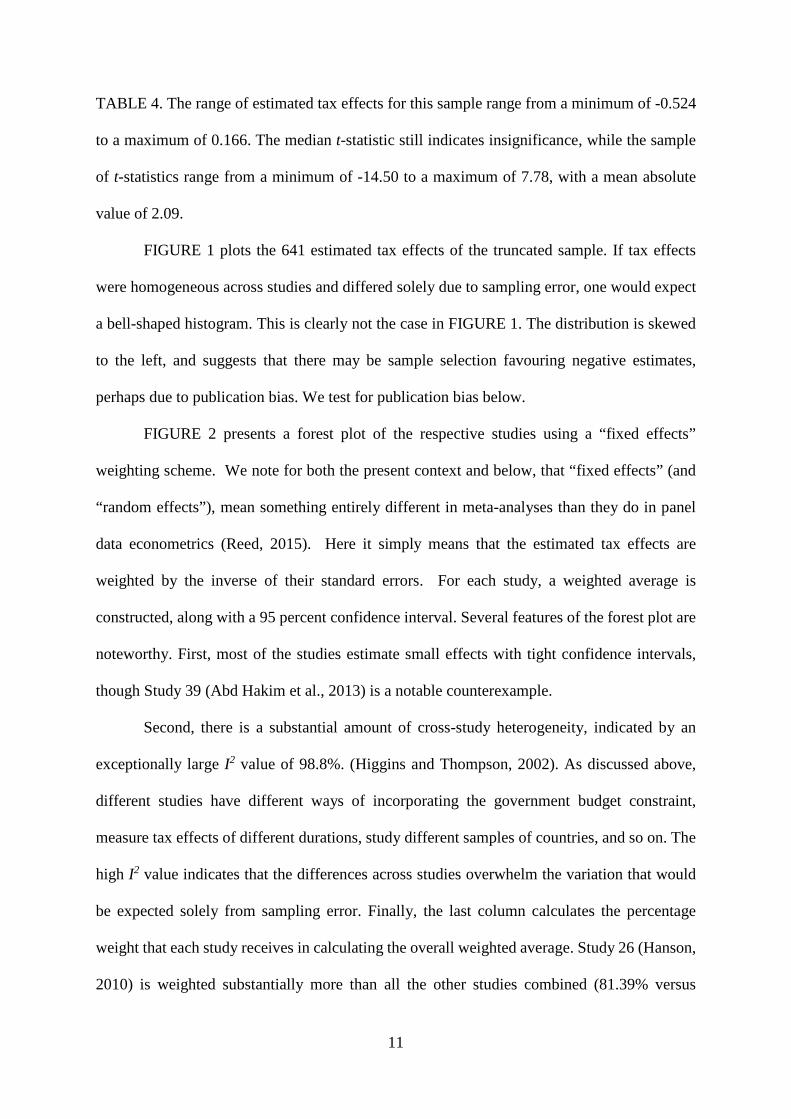
FIGURE 1 plots the 641 estimated tax effects of the truncated sample. If tax effects

were homogeneous across studies and differed solely due to sampling error, one would expect

a bell-shaped histogram. This is clearly not the case in FIGURE 1. The distribution is skewed

to the left, and suggests that there may be sample selection favouring negative estimates,

perhaps due to publication bias. We test for publication bias below.

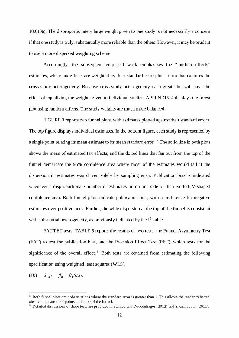
FIGURE 2 presents a forest plot of the respective studies using a “fixed effects”

weighting scheme. We note for both the present context and below, that “fixed effects” (and

“random effects”), mean something entirely different in meta-analyses than they do in panel

data econometrics (Reed, 2015). Here it simply means that the estimated tax effects are

weighted by the inverse of their standard errors. For each study, a weighted average is

constructed, along with a 95 percent confidence interval. Several features of the forest plot are

noteworthy. First, most of the studies estimate small effects with tight confidence intervals,

though Study 39 (Abd Hakim et al., 2013) is a notable counterexample.

Second, there is a substantial amount of cross-study heterogeneity, indicated by an

exceptionally large I2 value of 98.8%. (Higgins and Thompson, 2002). As discussed above,

different studies have different ways of incorporating the government budget constraint,

measure tax effects of different durations, study different samples of countries, and so on. The

high I2 value indicates that the differences across studies overwhelm the variation that would

be expected solely from sampling error. Finally, the last column calculates the percentage

weight that each study receives in calculating the overall weighted average. Study 26 (Hanson,

2010) is weighted substantially more than all the other studies combined (81.39% versus

12

18.61%). The disproportionately large weight given to one study is not necessarily a concern

if that one study is truly, substantially more reliable than the others. However, it may be prudent

to use a more dispersed weighting scheme.

Accordingly, the subsequent empirical work emphasizes the “random effects”

estimates, where tax effects are weighted by their standard error plus a term that captures the

cross-study heterogeneity. Because cross-study heterogeneity is so great, this will have the

effect of equalizing the weights given to individual studies. APPENDIX 4 displays the forest

plot using random effects. The study weights are much more balanced.

FIGURE 3 reports two funnel plots, with estimates plotted against their standard errors.

The top figure displays individual estimates. In the bottom figure, each study is represented by

a single point relating its mean estimate to its mean standard error.13 The solid line in both plots

shows the mean of estimated tax effects, and the dotted lines that fan out from the top of the

funnel demarcate the 95% confidence area where most of the estimates would fall if the

dispersion in estimates was driven solely by sampling error. Publication bias is indicated

whenever a disproportionate number of estimates lie on one side of the inverted, V-shaped

confidence area. Both funnel plots indicate publication bias, with a preference for negative

estimates over positive ones. Further, the wide dispersion at the top of the funnel is consistent

with substantial heterogeneity, as previously indicated by the I2 value.

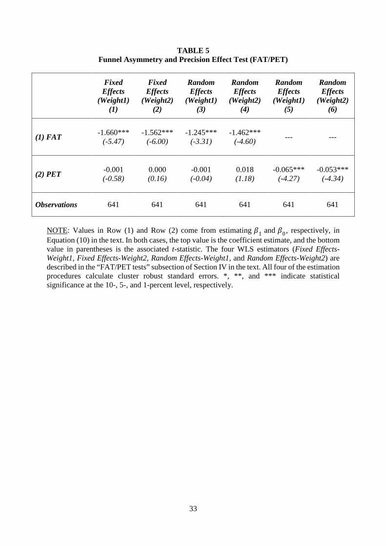
FAT/PET tests. TABLE 5 reports the results of two tests: the Funnel Asymmetry Test

(FAT) to test for publication bias, and the Precision Effect Test (PET), which tests for the

significance of the overall effect. 14 Both tests are obtained from estimating the following

specification using weighted least squares (WLS),

(10) 𝛼𝛼�1,𝐸𝐸𝑖𝑖 = 𝛽𝛽0 + 𝛽𝛽1𝑆𝑆𝐸𝐸𝐸𝐸𝑖𝑖,

13 Both funnel plots omit observations where the standard error is greater than 1. This allows the reader to better observe the pattern of points at the top of the funnel. 14 Detailed discussions of these tests are provided in Stanley and Doucouliagos (2012) and Shemilt et al. (2011).

13

where 𝛼𝛼�1,𝐸𝐸𝑖𝑖 is the estimated tax effect from regression j in study i. The null hypotheses for the

FAT and PET are 𝐻𝐻0:𝛽𝛽1 = 0 and 𝐻𝐻0:𝛽𝛽0 = 0, respectively.

Our analysis uses four different weights to estimate Equation (10). The Fixed

Effects(Weight1) and Random Effects(Weight1) estimators use weights � 1𝑆𝑆𝐸𝐸𝑖𝑖𝑖𝑖

� and

� 1

��𝑆𝑆𝐸𝐸𝑖𝑖𝑖𝑖�2+𝜏𝜏2

�, respectively, where 𝜏𝜏2 is the estimated variance of population tax effect

across studies. This set of weights makes no allowance for the fact that some studies report

more estimates than others. As a result, a study with 50 estimates is weighted 50 times more

than a study that reports a single estimate, ceteris paribus. To address this, we multiply both

sets of weights by � 1𝑁𝑁𝑖𝑖�, where 𝑁𝑁𝐸𝐸 is the number of estimated tax effects reported in study i.

The corresponding Fixed Effects(Weight2) and Random Effects(Weight2) estimators attempt to

give equal weight to each study regardless of the number of tax effects each study reports.

The first four columns of TABLE 5 report the results of estimating Equation (10) with

WLS, using the four different weighting schemes described above. The FAT is reported in the

first row. For all four estimators, the null hypothesis of no publication bias is rejected at the 1

percent level of significance. The negative coefficients indicate that sample selection favours

negative estimated tax effects, perhaps due to researchers choosing to disproportionately report

negative estimates, or journals discriminating against positive results. These results are

consistent with earlier observations about the histogram of estimated effects and the visual

evidence of publication bias from the funnel plots in FIGURE 3.

The first four columns of the second row of TABLE 5 report the PET. All four

estimators conclude that the overall tax effect, controlling for publication bias, is statistically

insignificant and relatively small in economic terms. For example, the Random

14

Effects(Weight1) estimate indicates that a ten percentage point increase in the tax rate is

associated with a 0.01 percentage point decrease in annual GDP growth.

The last two columns report random effects estimates of Equation (10) when the

publication bias term (𝑆𝑆𝐸𝐸𝐸𝐸𝑖𝑖) is not included, so that the overall estimate is not corrected for

publication bias. The corresponding estimates of the overall tax effects are now substantially

larger in absolute value, and statistically significant at the 1 percent level. According to the

Random Effects(Weight1) estimate in Column (5), a ten percentage point increase in the tax

rate is associated with a 0.65 percentage point decrease in annual GDP growth. These results

indicate that the statistically and economically significant results reported in the literature are

a consequence of publication bias that favours negative estimates of tax effects, while

suppressing the publication of positive tax effects. As a result, we want to be sure that our

subsequent analysis corrects for this.

This section has addressed the first goal of this research, to obtain an “overall estimate”

of the effect of taxes on economic growth in OECD countries. We find that a publication-bias

adjusted estimate of the overall effect on taxes is statistically insignificant and negligibly small

in economic terms. However, our previous discussion on factors that cause tax estimates to

differ across studies (cf. Section III) makes clear that any estimate of overall tax effects is not

particularly meaningful. The same fiscal policy action can be estimated as a positive or negative

tax effect depending on the elements of the government budget constraint that are omitted from

the original study’s regression equation. Accordingly, the next section undertakes a meta-

regression that allows tax effects to vary systematically according to study and data

characteristics.

Meta-regression. Section III identified a large number of factors that can affect the

estimated size of tax effects. In this section, we compare tax effects associated with fiscal

policies that are predicted to have negative growth effects, with those predicted to have positive

15

effects. We also investigate whether some types of taxes are more growth-retarding than

others. To do that, it will be necessary to control for the myriad other factors that impact

estimates of tax effects.

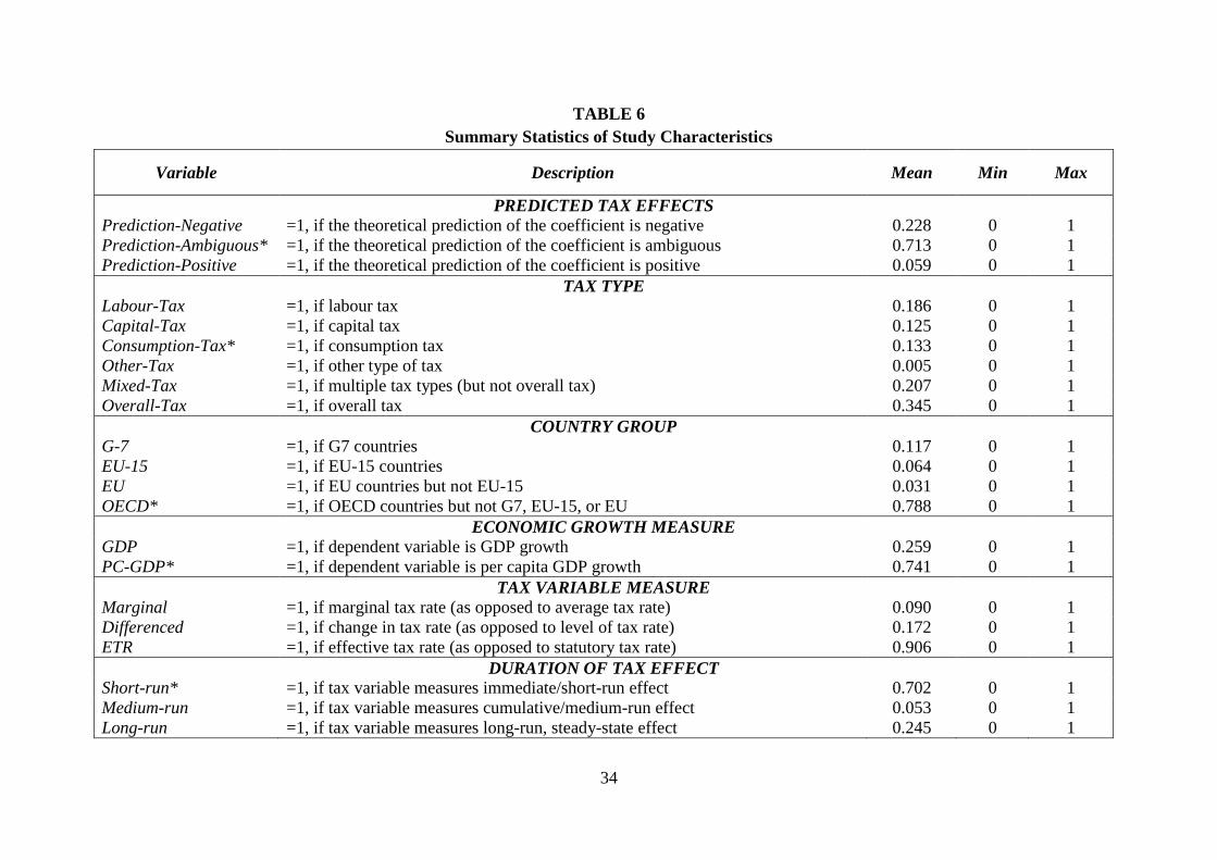
TABLE 6 reports the variables used in the subsequent meta-regression analysis. The

first set of variables were previously discussed and match each tax effect to a prediction. A

little more than a fourth of the estimated tax effects allow a definite sign prediction, with 22.8

percent predicted to be negative, 5.9 percent predicted to be positive, and the rest ambiguous.

As these three variables comprise the full set of possibilities, at least one variable must be

omitted in the empirical analysis. Here and elsewhere we indicate the omitted variable with an

asterisk.

The second set of variables assigns each tax effect to one of six types of taxes (Labour,

Capital, Consumption, Other, Mixed, and Overall). The most common tax variable is

constructed by taking the ratio of total tax revenues over GDP. 34.5 percent of tax effects are

of this type. However, many studies disaggregate tax effects into separate types. 18.6 percent

of estimated tax effects involve Labour taxes (e.g., personal income taxes, payroll taxes, social

security contributions). Another 12.5 percent are associated with Capital taxes (e.g., corporate

income taxes, taxes on capital gains and dividends). 13.3 percent are related to Consumption

taxes (e.g., ad valorem taxes on goods and services, VAT). The remainder of tax effects mostly

involve a mix of different tax types.

Subsequent variables are grouped into numerous categories: Country Group, Economic

Growth Measure, Tax Variable Measure, Duration of Tax Effect, etc. Most of the observed tax

effects are estimated using data from the larger set of OECD countries (78.8%), as opposed to

smaller groupings such as the G-7 countries (11.7%) or EU countries (6.4% and 3.1%). In most

cases, economic growth is measured in per capita terms (74.1%). Most taxes are measured as

average rates, rather than marginal (91.0% versus 9.0%); are specified in level rather than

16

differenced form (82.8% versus 17.2%); and are effective rather than statutory tax rates (90.6%

versus 9.4%). Most estimated tax effects measure the immediate effect of a tax change (70.2%),

versus a medium- or long-run effect (5.3% and 24.5%).

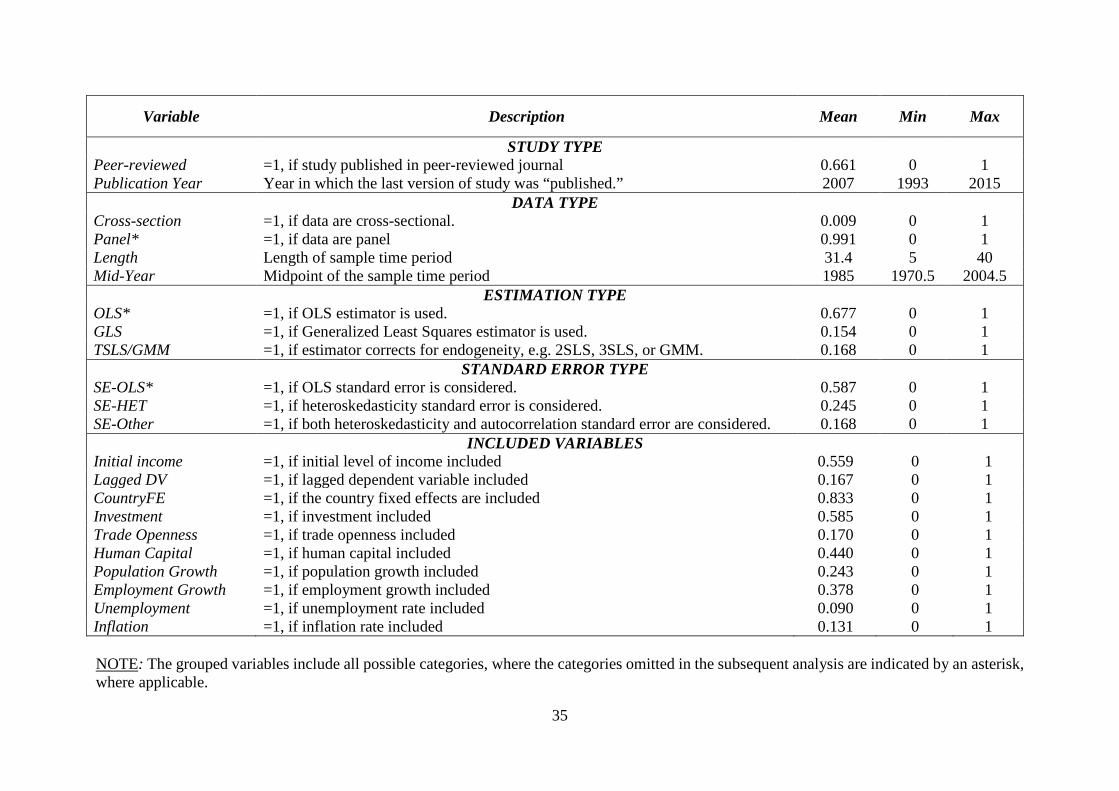
Two thirds of the estimated tax effects in our meta-regression come from peer-reviewed

journal articles and the mean year of publication was 2007. Almost all of the original studies

used panel data to estimate tax effects (99.1%). The average sample length in the original

studies was 31.4 years, and the average mid-point was 1985. About two-thirds of the tax effects

were estimated using OLS or a related procedure that assumed errors to be independently and

identically distributed across observations (such as mean group or pooled mean group

procedures). Of the remainder, 15.4 percent used GLS, and 16.8 percent attempted to correct

for endogeneity using a procedure such as TSLS or GMM.

Because the standard error plays such a significant role in meta-analysis, we categorized

standard errors into three groupings: SE-OLS (58.7%); SE-HET (24.5%), where standard errors

were estimated using a heteroskedastic-robust estimator; and SE-Other (16.8%), whenever

allowance was made for off-diagonal terms in the error variance-covariance matrix to be

nonzero. Lastly, dummy variables were used to indicate the presence of important control

variables, the most common of which were country fixed effects (83.3%), and measures of

investment (58.5%), initial income (55.9%), human capital, such as educational achievement

(44.0%), employment growth (37.8%), and population growth (24.3%).

In our investigation of tax effects, we adopt the following empirical procedure. First we

separate out the two sets of tax variables: Prediction-Negative and Prediction-Positive; and

Labour-Tax, Capital-Tax, Other-Tax, Mixed-Tax, and Overall-Tax. We do this because the two

sets of tax variables are significantly correlated. For example, Labour and Capital taxes are

significantly associated with tax policies that are predicted to have negative effects. We then

combine the two sets of tax variables to check for robustness.

17

For each set of regressions we also include two sets of control variables. The top panel

of each table reports the regression results when all control variables are included in the

equation. The bottom panel reports the results when a stepwise procedure is used to select

control variables, even while the tax variables are fixed to remain in each equation.15 Since the

tax variables are locked into each regression, the use of the stepwise procedure does not

invalidate their significance testing. All regressions also include the publication bias variable,

SE, and thus control for publication bias.

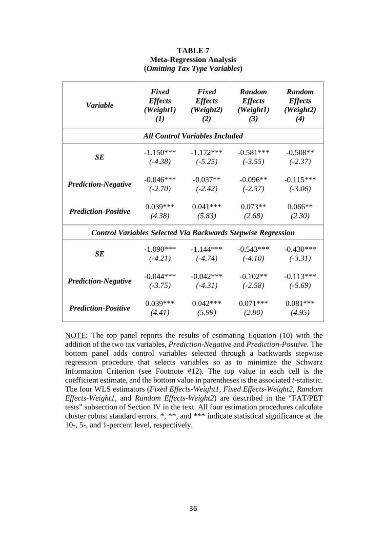
The results of this analysis are given in TABLES 7 through 9. TABLE 7 reports the

results when the prediction variables (Prediction-Negative and Prediction-Positive) are

included in the meta-regression, while holding out the tax type variables. Across all four

estimation procedures, and for both sets of control variables, we estimate a negative and

statistically significant coefficient for the variable Prediction-Negative, and a positive and

statistically significant coefficient for Prediction-Positive. These results are consistent with the

prediction of growth theory.

The results are only slightly less supportive of growth theory when the tax type

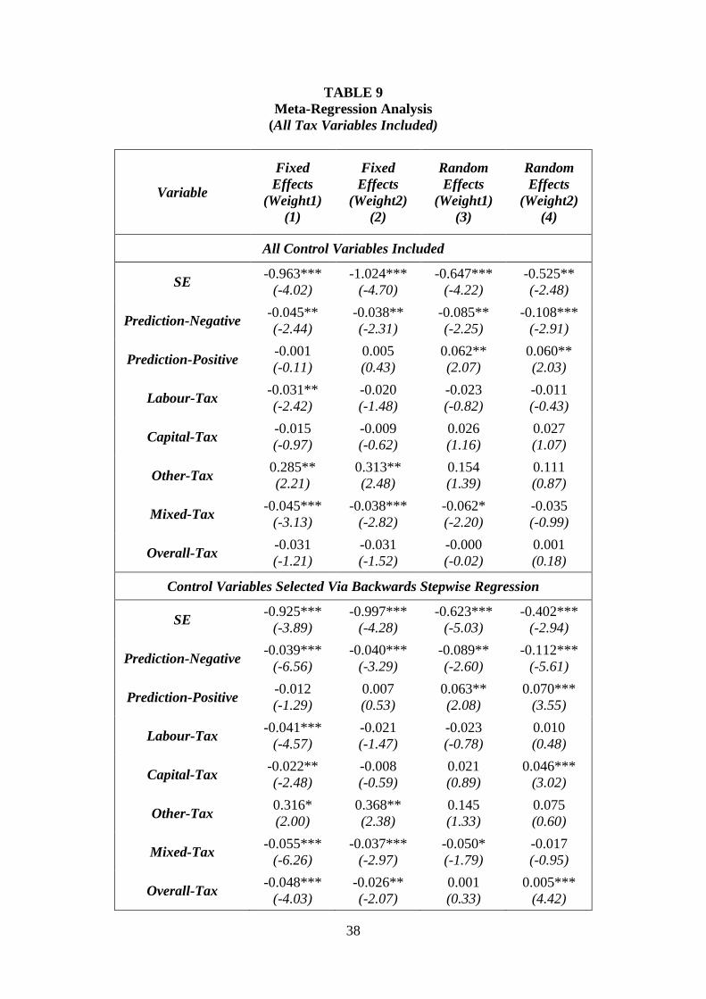
variables are added to the specification. TABLE 9 reports the corresponding estimates. The

coefficient for Prediction-Negative remains negative and statistically significant across all four

estimation procedures. Prediction-Positive is positive and statistically significant in the two

random effects regressions (Columns 3 and 4), but insignificant in the two fixed effects

regressions (Columns 1 and 2). As noted above, we consider the random effects estimator to

be more reliable, so that the results from TABLE 9 are generally consistent with those from

TABLE 7.

15 We use a backwards stepwise regression procedure that selects variables so as to minimize the Schwarz Information Criterion. We employed the user-written, Stata program vselect to implement the stepwise procedure.

18

Not only do these findings constitute general statistical support in favour of the

predictions of growth theory, but the respective coefficients indicate that tax policy can have a

substantial economic impact. For example, the difference between the coefficients for

Prediction-Negative and Prediction-Positive range from a minimum of 0.027 (TABLE 9,

Bottom panel, Column 1) to a maximum of 0.194 (TABLE 7, Bottom panel, Column 4), with

a midpoint value of approximately 0.11.

Let us now consider the following thought experiment: Suppose fiscal policy

underwent the following policy switch. Distortionary taxes and unproductive expenditures

were reduced by 10 percentage points while, simultaneously, non-distortionary taxes and

productive expenditures were increased by the same amount. Using a point estimate of 0.11,

our meta-regression results indicate that this would increase annual growth of GDP by 1.1

percentage points. As noted above, the average annual growth rate for OECD countries over

the sample range of the studies included in this meta-analysis was approximately 2.5 percent.

Thus a 1.1 percentage point increase in annual growth would constitute a substantial increase.

Admittedly, this thought experiment is an extreme case, both in the absolute size of the tax

changes, and in the swing in fiscal policy from one extreme of the growth pole to the other.

Nevertheless, it does indicate that there is a role for tax-based fiscal policy to increase economic

growth amongst OECD countries.

The last tax issue addressed in this study investigates whether some types of taxes are

more growth-retarding than others. As noted in TABLE 1, Labour and Capital taxes are

commonly classified as distortionary, while Consumption taxes are classified as non-

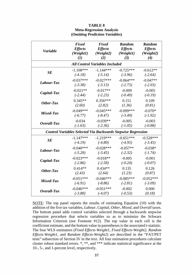
distortionary. TABLE 8 estimates a meta-regression with the tax type variables but with

prediction variables omitted, while TABLE 9 includes both. As the omitted category is

Consumption taxes, we expect the coefficient on Labour and Capital taxes to be negative,

whereas there is no sign expectation for the other tax type coefficients.

19

With respect to Labour taxes, the results from TABLE 8, across all four estimation

procedures and with both sets of control variables, show negative and statistically significant

coefficients. However, when prediction variables are added to the regression (cf. TABLE 9),

the coefficient on Labour-Tax becomes insignificant in the preferred random effects

regressions. In terms of economic significance, the estimates range from -0.064 (TABLE 8,

Top panel, Column 3) to 0.010 (TABLE 9, Bottom panel, Column 4). The more negative

estimates indicate that raising revenues from Labour taxes rather than Consumption taxes can

have important growth consequences. However, given that some of the preferred Random

Effects estimates are statistically insignificant, our overall assessment is that these estimates

constitute weak evidence that Labour taxes are more growth-retarding than Consumption taxes.

The evidence that Capital taxes are more distortionary than Consumption taxes is even

weaker. While the coefficients on the Capital-Tax variable are negative in all TABLE 8

regressions, they are insignificant in the preferred random effects estimations. When the

prediction variables are added, the respective coefficients are generally insignificant (cf.

TABLE 9). One of the regressions even produces a significant positive coefficient (bottom

panel, Random Effects-Weight2). As a result, we conclude that the evidence that Capital taxes

are more distortionary than Consumption taxes is mixed.

Bayesian model averaging of control variables. Having addressed the major goals of

this study, we turn to an analysis of the control variables. Not counting the two sets of tax

variables, there are 28 control variables. With so many variables, multicollinearity is a problem.

For example, when all 28 variables are included with both sets of tax variables and the meta-

regression is estimated using the Random Effects(Weight2) estimator, as in Column (4) of the

top panel of TABLE 9, 5 of the 28 control variables are significant at the 5 percent level. When

the backwards stepwise routine is employed, as in the bottom panel of TABLE 9, 9 of the 28

control variables are significant. One of the variables that is significant in the top panel is not

20

significant in the bottom panel’s specification. Thus, variable selection makes a difference.

This was not so much a problem when we estimated tax effects, because the variables were

locked into the respective specifications without regard to statistical significance. However, it

is a problem when trying to decide which control variables to include in the specification.

We use Bayesian Model Averaging (BMA) to address this issue (Zeugner, 2011).

TABLE 10 reports the results of an analysis where we lock in the tax variables Prediction-

Negative and Prediction-Positive and then apply BMA to the 28 control variables. All

specifications adjust for publication bias. The results differ somewhat depending on the

estimation procedure used. However, they are more consistent across analyses than would be

the case, say, if we reported the results from specifications that included all variables and those

that employed stepwise regression. We report results for both the Fixed Effects(Weight1) and

Random Effects(Weight2) estimators. These two estimators use very different weighting

schemes. Previous tables indicated that the estimates from these two estimators sometimes vary

substantially. As a result, they provide an indication of robustness across estimation

procedures.

We report three summary measures. The Posterior Inclusion Probability (PIP) is a

weighted probability that uses the likelihood values of specifications to construct a

“probability” that a given specification is “true”. With 28 control variables, there are 1028

possible variable specifications. Variables that appear in specifications with high likelihood

values will have larger PIP values. By construction, every variable appears in 50 percent of all

possible specifications. However, the PIP can be very close to 100 percent if the specifications

that include a variable have much greater likelihood values than those in which it is omitted.

The Posterior Mean (Post. Mean) uses the above-mentioned probability values to

weight the estimated coefficients from each specification. Specifications in which a variable is

not included assign an “estimated value” of zero to construct the Posterior Mean. Lastly, BMA

21

also calculates the probability that a given coefficient has a positive sign (Cond. Pos. Sign).

This is constructed in the same manner as the Posterior Mean, except that it uses a dummy

variable indicating positive value rather than the estimated coefficient in constructing a

weighted average.

TABLE 10 yellow highlights all the control variables that (i) have a PIP greater than

50%; (ii) have a Conditional Positive Sign of either 1.00 or 0.00 – indicating that the respective

coefficient is consistently estimated to be either positive or negative in the most likely

specifications; and (iii) have the same Conditional Positive Sign value for both the Fixed

Effects(Weight1) and Random Effects(Weight2) estimators.

Studies that estimate tax effects for G-7 and EU-15 countries produce consistently less

negative/more positive estimates than studies that include a large sample of countries from the

OECD. To place the size of the Posterior Mean values in context, it helpful to recall that the

median estimated tax effect from TABLE 4 is -0.073. By this standard, the effect of belonging

to a G-7 country is relatively large (0.184 and 0.181, respectively). The effect associated with

being a EU-15 member, while still positive, is substantially smaller.

We find that studies that measure economic growth using total GDP (GDP) rather than

per capital GDP, and that employ a marginal (as opposed to average) measure of tax rates

(Marginal), generally produce tax effects that are less negative/more positive. Compared to the

short-run effects of taxes, studies that estimate medium-run tax effects (Medium-run) produce

estimates of tax effects that less negative/more positive; while studies that estimate long-run,

steady-state tax effects (Long-run) produce estimates that are more negative/less positive.

There is evidence to indicate that more recent studies (Publication Year) produce less

negative/more positive estimates; as do cross-sectional studies (Cross-section) compared to

panel studies. However, there is also evidence that studies using more recent data (Mid-Year)

find more negative/less positive tax effects.

22

With respect to estimation procedures, studies that use GLS rather than OLS (GLS),

generally produce more negative/less positive estimates of tax effects. Interestingly, correcting

for endogeneity (TSLS/GMM) does not appear to have much impact. Meta-regressions using

the Fixed Effects(Weight1) estimator find that studies that employ TSLS/GMM generally

estimate more negative/less positive effects. Meta-regressions using the Random

EffectsWeight2) estimator find the opposite. However, in both cases, the Posterior Mean values

are negligibly small (-0.001 and 0.009), suggesting either that tax policy is not endogenous, or

that the instruments that have been employed in previous studies are not effective in correcting

endogeneity. There is evidence that it makes a difference how one calculates standard errors,

with studies that incorporate serial correlation, cross-sectional correlation and the like in

calculating standard errors (SE-Other) associated with less negative/more positive effects.

Lastly, we find that studies that include initial income, employment growth, and

unemployment rates in the growth equations are likely to produce less negative/more positive

estimates; with studies that include country fixed effects, population growth, and inflation

producing more negative/less positive tax effects. While the above findings are robust across

variable specifications and the two estimation procedures, we again emphasize that the sizes of

the associated effects, like those of tax policy itself, are small.

FIGURE 4 provides a visual representation of the BMA analysis for the tax (Prediction-

Negative and Prediction-Positive) and control variables using the Fixed Effects(Weight1)

estimator.16 The figure reports estimates from the top 1000 models, with most likely models

ordered from left to right. These 1000 models, out of 1028 possible models, account for a

cumulative probability of approximately 30 percent. Red (blue) squares indicate that the

respective coefficient is negative (positive) in the given model. A white square indicates that

16 Note that in the associated specifications, the variable Precision corresponds to the constant term, while the constant term corresponds to the publication bias variable, SE.

23

the variable is omitted from that model. A solid band of the same colour across the figure

indicates that the respective variable is consistently estimated to have the same sign across all

1000 models. In addition to confirming the results from TABLE 10, the figure also indicates

the variable specifications of the top models. These closely match the PIP values in TABLE

10. The corresponding figure for the Random Effects(Weight2) estimator is quite similar, and

is reproduced in APPENDIX 5.

V. CONCLUSION

The literature on taxes and economic growth in OECD countries has produced a large

number of frequently conflicting estimates. One reason for the seemingly contradictory

findings is that estimates of tax effects are often estimating different things. Because of the

government budget constraint, the same tax effect can be estimated to be positive or negative,

depending on the other budget categories omitted from the specification. For this and other

reasons, it is valuable to collect the estimates from this literature and carefully track the

differences across studies so that the estimates can be combined to provide an overall

assessment of the growth effects of taxes.

This study combines results from 42 studies containing 713 estimates, all which

endeavour to estimate the effect of taxes on economic growth in OECD countries. We drop

extreme estimates from both ends of the sample range, and use meta-analysis to analyse a final

sample of 641 estimates. We find that estimates in the literature are characterized by significant

(negative) publication bias. Controlling for publication bias, the overall effect of taxes on

economic growth is negligibly small and statistically insignificant. However, this overall effect

is not particularly meaningful because it mixes together many different kinds of tax policies.

To get a better idea of the scope of tax policy to effect economic growth, we categorize

tax policies by their predicted effects on economic growth. We estimate that, after adjusting

for publication bias, increases in unproductive expenditures funded by distortionary taxes

24

and/or deficits have a statistically significant, negative effect on economic growth. In contrast,

increases in non-distortionary taxes to fund productive expenditures and/or government

surpluses have a statistically significant, positive effect on economic growth. The difference

between these “best” and “worst” tax policies can be economically important. For example,

using a midpoint estimate from our meta-regression analysis, we calculate that if distortionary

taxes and unproductive expenditures were reduced by 10 percentage points while,

simultaneously, non-distortionary taxes and productive expenditures were increased by the

same amount, the net effect would be an increase of 1.1 percentage points in annual GDP

growth. While this represents an extreme case, both in the absolute size of the tax changes, and

in the swing in fiscal policy from one extreme of the growth pole to the other, it does indicate

that there is scope for tax-based fiscal policy to increase economic growth.

With respect to particular types of taxes, we find weak evidence that taxes on labour

are more growth retarding than other types of taxes. Evidence regarding other types of taxes is

mixed. Finally, we find evidence that data and study characteristics account for much

systematic variation in tax estimates across studies, though the effects from any one

characteristic is generally small. The one exception is that studies that focus their analysis on

G-7 countries find less negative/more positive tax effects than those that use a wider sample of

OECD countries.

One of the advantages of meta-analysis is that it can avoid some of the pitfalls

associated with publication bias and selective reporting of results. Further, it can control for

differences across studies that might otherwise mask significant effects. This is particularly

relevant when estimating the effects of tax policy. The results of this study indicate that when

these factors are taken into account, the combined weight of the evidence from the literature

indicates that tax policy can have an economically important impact on economic growth.

25

REFERENCES

Afonso, A., and Alegre, J. G. (2008). Economic growth and budgetary components: A panel

assessment for the EU. Working Paper Series 848, European Central Bank, Frankfurt. Afonso, A., and Alegre, J. G. (2011). Economic growth and budgetary components: A panel

assessment for the EU. Empirical Economics, 41(3), 703-723. Afonso, A., and Furceri, D. (2010). Government size, composition, volatility and economic

growth. European Journal of Political Economy, 26(4), 517-532. Afonso, A., and Jalles, J. T. (2014). Fiscal composition and long-term growth. Applied

Economics, 46(3), 349-358. Afonso, A., and Jalles, J. T. (2013). Fiscal composition and long-term growth.Working Paper

Series 1518, European Central Bank, Frankfurt. Agell, J., Lindh, T., and Ohlsson, H. (1997). Growth and the public sector: A critical review

essay. European Journal of Political Economy, 13(1), 33-52. Agell, J., Lindh, T., and Ohlsson, H. (1999). Growth and the public sector: A reply. European

Journal of Political Economy, 15(2), 359-366. Agell, J., Ohlsson, H., and Thoursie, P. S. (2006). Growth effects of government expenditure

and taxation in rich countries: A comment. European Economic Review, 50(1), 211-218.

Alesina, A., and Ardagna, S. (2010). Large changes in fiscal policy: Taxes versus spending.

Tax Policy and the Economy, 24, 35-68. Angelopoulos, K., Economides, G., and Kammas, P. (2007). Tax-spending policies and

economic growth: Theoretical predictions and evidence from the OECD. European Journal of Political Economy, 23(4), 885-902.

Arin, K. P. (2004). Fiscal Policy, Private Investment and Economic Growth: Evidence from G-

7 Countries. Unpublished manuscript. Arnold, J. M. (2008). Do tax structures affect aggregate economic growth? Empirical evidence

from a panel of OECD countries. Working Paper Series 643, Organization for Economic Co-operation and Development. Economic Department of the OECD.

Arnold, J. M., Brys, B., Heady, C., Johansson, Å., Schwellnus, C., and Vartia, L. (2011). Tax

policy for economic recovery and growth. The Economic Journal, 121(550), F59-F80. Bania, N., Gray, J.A., and Stone, J.A. (2007). Growth, taxes, and government expenditures:

Growth hills for U.S. states. National Tax Journal, Vol. LX(2), 193-204. Barro R. (1990) Government spending in a simple model of endogenous growth, Journal of

Political Economy, 98, s103-117.

26

Barro, R. and Sala-i-Martin, X. (1992) Public finance in models of economic growth, Review of Economic Studies, 59, 645-61.

Baskaran, T., and Feld, L. P. (2013). Fiscal decentralization and economic growth in OECD

countries: Is there a relationship?. Public Finance Review, 41(4), 421-445. Bassanini, A., Scarpetta, S., and Hemmings, P. (2001). Economic growth: the role of policies

and institutions. Panel data evidence from OECD countries. Benos, N. (2009). Fiscal policy and economic growth: Empirical evidence from EU

countries. Working Paper Series 107. Center for Planning and Economic Research. Bergh, A., and Karlsson, M. (2010). Government size and growth: Accounting for economic

freedom and globalization. Public Choice, 142(1-2), 195-213. Bergh, A., and Öhrn, N. (2011). Growth effects of fiscal policies: A critical appraisal of

Colombier’s (2009) study. Working Paper Series 865, Research Institute of Industrial Economics (IFN).

Bleaney, M., Gemmell, N., and Kneller, R. (2001). Testing the endogenous growth model:

Public expenditure, taxation, and growth over the long run. Canadian Journal of Economics/Revue canadienne d'économique, 34(1), 36-57.

Colombier, C. (2009). Growth effects of fiscal policies: An application of robust modified M-

estimator. Applied Economics, 41(7), 899-912. Dackehag, M., and Hansson, Å. (2012). Taxation of income and economic growth: An

empirical analysis of 25 rich OECD countries. Working Paper Series 2012:6, Lund University.

Daveri, F., and Tabellini, G. (2000). Unemployment, growth and taxation in industrial

countries. Economic Policy, 15(30), 47-104. De la Fuente, A. (1997). Fiscal policy and growth in the OECD. Discussion Paper Series 1755,

Center for Economic Policy Research (CEPR). Devarajan S., Swaroop, V., and Zou, H. (1996) The composition of public expenditure and

economic growth, Journal of Monetary Economics, 37, 313-344. Fölster, S., and Henrekson, M. (1999). Growth and the public sector: A critique of the

critics. European Journal of Political Economy, 15(2), 337-358. Fölster, S., and Henrekson, M. (2001). Growth effects of government expenditure and taxation

in rich countries. European Economic Review,45(8), 1501-1520. Futagami, K.Y, Morita, Y., and Shibata, A. (1993) Dynamic analysis of an endogenous growth

model with public capital, Scandinavian Journal of Economics, 95, 606-625. Furceri, D., and Karras, G. (2009). Tax changes and economic growth: Empirical evidence for

a panel of OECD countries. Unpublished manuscript.

27

Gemmell, N., Kneller, R., and Sanz, I. (2008). Fiscal policy impacts on growth in the OECD: Are they long-run?. Mimeo, University of Nottingham.

Gemmell, N., Kneller, R., and Sanz, I, (2009). The composition of government expenditure

and economic growth: some new evidence for OECD countries. In European Commission, The quality of public finances and economic growth: Proceedings to the annual workshop on public finances (Brussels, 28 November 2008), European Economy, Occasional Papers No. 45. Directorate-General for Economic and Financial Affairs, Publications, Brussels, Belgium, pages 17-46.

Gemmell, N., Kneller, R., and Sanz, I. (2011). The timing and persistence of fiscal policy

impacts on growth: Evidence from OECD countries. The Economic Journal, 121(550), F33-F58.

Gemmell, N., Kneller, R., and Sanz, I. (2014). The growth effects of tax rates in the

OECD. Canadian Journal of Economics/Revue Canadienne d'Economique, 47(4), 1217-1255.

Gemmell, N., Kneller, R., and Sanz, I. (2015). Does the Composition of Government

Expenditure Matter for Long‐Run GDP Levels?. Oxford Bulletin of Economics and Statistics. DOI: 10.1111/obes.12121

Hakim, T. A., Bujang, I., and Ahmad, I. (2013) Tax structure and economic indicators in the

modern era: Developing vs. high-income OECD countries. Conference paper. Hansson, Å. (2010). Is the wealth tax harmful to economic growth? World Tax Journal, 2(1),

19-34. Havranek, T., and Irsova, Z. (2012). Survey article: Publication bias in the literature on foreign

direct investment spillovers. The Journal of Development Studies, 48(10), 1375-1396. Heitger, B. (1993). Convergence, the “tax-state” and economic dynamics. Weltwirtschaftliches

Archiv, 129(2), 254-274. Higgins, J.P. and Thompson, S.G. (2002). Quantifying heterogeneity in a meta-analysis.

Statistics in Medicine, 21(11), 1539-58. Karras, G. (1999). Taxes and growth: Testing the neoclassical and endogenous growth

models. Contemporary Economic Policy, 17(2), 177-188. Karras, G., and Furceri, D. (2009). Taxes and growth in Europe. South-Eastern Europe Journal

of Economics, 2, 181-204. Kneller, R., Bleaney, M. F., and Gemmell, N. (1999). Fiscal policy and growth: Evidence from

OECD countries. Journal of Public Economics, 74(2), 171-190. Mendoza, E. G., Milesi-Ferretti, G. M., and Asea, P. (1997). On the ineffectiveness of tax

policy in altering long-run growth: Harberger's superneutrality conjecture. Journal of Public Economics, 66(1), 99-126.

28

Miller, S. M., and Russek, F. S. (1997). Fiscal structures and economic growth: International evidence. Economic Inquiry, 35(3), 603-613.

Muinelo-Gallo, L., and Roca-Sagalés, O. (2013). Joint determinants of fiscal policy, income

inequality and economic growth. Economic Modelling, 30, 814-824. Padovano, F., and Galli, E. (2001). Tax rates and economic growth in the OECD

countries. Economic Inquiry, 39(1), 44-57. Paparas, D., Richter, C., and Paparas, A. (2015). Fiscal Policy and Economic Growth,

Empirical Evidence in European Union. Turkish Economic Review,2(4), 239-268. Reed, W.R. (2015). A Monte Carlo analysis of alternative meta-analysis estimators in the

presence of publication bias. Economics: The Open-Access, Open-Assessment E-Journal, 9(2015-30): 1-40.

Romero-Avila, D., and Strauch, R. (2008). Public finances and long-term growth in Europe:

Evidence from a panel data analysis. European Journal of Political Economy, 24(1), 172-191.

Shemilt, I., Mugford, M., Vale, L., Marsh, K. and Donaldson, C., (eds.) (2011). Evidence-based

decisions and economics: Health care, social welfare, education, and criminal justice, 2nd edition. New York: John Wiley & Sons.

Stanley, T.D., and Doucouliagos, H. (2012). Meta-regression analysis in economics and

business. London: Routledge. Stanley, T.D., Doucouliagos, H., Giles, M., Heckemeyer, J.H., Johnston, R.J., Laroche, P.,

Nelson, J.P., Paldam, M., Poot, J., Pugh, G. and Rosenberger, R.S. (2013). Meta-analysis of economics research reporting guidelines. Journal of Economic Surveys, 27(2), 390-394.

Volkerink, B., Sturm, J. E., and De Haan, J. (2002). Tax ratios in macroeconomics: Do taxes

really matter? Empirica, 29(3), 209-224. Widmalm, F. (2001). Tax structure and growth: Are some taxes better than others? Public

Choice, 107(3-4), 199-219. Xing, J. (2011). Does tax structure affect economic growth? Empirical evidence from OECD

countries. Working Paper Series 11/20. Center for Business Taxation, Said Business School, University of Oxford.

Xing, J. (2012). Tax structure and growth: How robust is the empirical evidence? Economics

Letters, 117(1), 379-382. Zeugner, S. (2011). Bayesian model averaging with BMS. Available at http://bms.zeugner.eu/

[Accessed 15 Oct. 2015].

29

TABLE 1 Matching of Functional and Theoretical Classifications

Functional classification Theoretical classification

Taxation on income and profit

Distortionary taxation

Social security contributions

Taxation on payroll and manpower

Taxation on property

Taxation on domestic goods and services Non-distortionary taxations

Taxation on international trade Other revenues

Non-tax revenues

Other tax revenues

General public services expenditure

Productive expenditures

Defense expenditure

Educational expenditure

Health expenditure

Housing expenditure

Transport and communication expenditure

Social security and welfare expenditure Unproductive expenditures

Expenditure on recreation

Expenditure on economic services

Other expenditures (unclassified) Other expenditures

NOTE: The categorizations in the table are taken from Kneller, Bleaney, and Gemmell (1999).

30

TABLE 2 Predicted Tax Effects

Type of Tax Omitted Fiscal Category Predicted Effect

Distortionary Productive Expenditures Ambiguous

Distortionary Unproductive expenditures Negative

Distortionary All the expenditures( Pro&Unpro) Ambiguous

Distortionary Other Expenditures Ambiguous

Distortionary Deficit/Surplus Ambiguous

Distortionary Other Revenue Ambiguous

Distortionary Distortionary Taxes Ambiguous

Distortionary Non-distortionary Taxes Negative

Distortionary Intergovernmental Revenue Ambiguous

Distortionary Net Utility Expenditures Ambiguous

Non-distortionary Productive Expenditures Positive

Non-distortionary Unproductive Expenditures Ambiguous

Non-distortionary Productive & Unproductive Expenditures Ambiguous

Non-distortionary Other Expenditures Ambiguous

Non-distortionary Deficit/Surplus Positive

Non-distortionary Other Revenue Ambiguous

Non-distortionary Distortionary Taxes Positive

Non-distortionary Non-distortionary Taxes Ambiguous

Non-distortionary Intergovernmental Revenue Ambiguous

Non-distortionary Net Utility Expenditures Ambiguous NOTE: The categorizations in the table are taken from Gemmell, Kneller, and Sanz (2009), where we combine the original categories of “zero” and “ambiguous” to “ambiguous”.

31

TABLE 3 Types of Taxes

Tax Type Examples

Labour Personal income tax Payroll tax Social security contributions

Capital Corporate income tax Capital tax (tax on dividends)

Consumption

Consumption tax Taxes on goods and services Sales tax Value added tax (VAT) International trade tax

Other tax Property tax Taxes not listed above

Mixed tax Taxes that are a combination of the above types

Overall tax Total taxes (e.g., Total Tax Revenues/GDP)

32

TABLE 4 Descriptive Statistics for Estimated Effects and t-statistics

Estimated Tax Effects t-statistics

Full Truncated Full Truncated

Mean -0.097 -0.109 2.16* 2.09*

Median -0.073 -0.073 -1.27 -1.32

Minimum -3.520 -0.524 -14.50 -14.50

Maximum 12.720 0.166 8.03 7.78

Std. Dev. 0.649 0.147 2.49 2.35

1% -1.320 -0.480 -7.91 -8.29

5% -0.530 -0.420 -6.17 -6.18

10% -0.411 -0.342 -4.72 -4.72

90% 0.078 0.041 1.07 0.67

95% 0.167 0.082 1.67 1.25

99% 0.820 0.143 4.59 3.09

Obs 713 641 713 641

33

TABLE 5 Funnel Asymmetry and Precision Effect Test (FAT/PET)

Fixed Effects

(Weight1) (1)

Fixed Effects

(Weight2) (2)

Random Effects

(Weight1) (3)

Random Effects

(Weight2) (4)

Random Effects

(Weight1) (5)

Random Effects

(Weight2) (6)

(1) FAT -1.660*** (-5.47)

-1.562*** (-6.00)

-1.245*** (-3.31)

-1.462*** (-4.60) --- ---

(2) PET -0.001 (-0.58)

0.000 (0.16)

-0.001 (-0.04)

0.018 (1.18)

-0.065*** (-4.27)

-0.053*** (-4.34)

Observations 641 641 641 641 641 641

NOTE: Values in Row (1) and Row (2) come from estimating 𝛽𝛽1 and 𝛽𝛽0, respectively, in Equation (10) in the text. In both cases, the top value is the coefficient estimate, and the bottom value in parentheses is the associated t-statistic. The four WLS estimators (Fixed Effects-Weight1, Fixed Effects-Weight2, Random Effects-Weight1, and Random Effects-Weight2) are described in the “FAT/PET tests” subsection of Section IV in the text. All four of the estimation procedures calculate cluster robust standard errors. *, **, and *** indicate statistical significance at the 10-, 5-, and 1-percent level, respectively.

34

TABLE 6 Summary Statistics of Study Characteristics

Variable Description Mean Min Max

PREDICTED TAX EFFECTS Prediction-Negative =1, if the theoretical prediction of the coefficient is negative 0.228 0 1 Prediction-Ambiguous* =1, if the theoretical prediction of the coefficient is ambiguous 0.713 0 1 Prediction-Positive =1, if the theoretical prediction of the coefficient is positive 0.059 0 1

TAX TYPE Labour-Tax =1, if labour tax 0.186 0 1 Capital-Tax =1, if capital tax 0.125 0 1 Consumption-Tax* =1, if consumption tax 0.133 0 1 Other-Tax =1, if other type of tax 0.005 0 1 Mixed-Tax =1, if multiple tax types (but not overall tax) 0.207 0 1 Overall-Tax =1, if overall tax 0.345 0 1

COUNTRY GROUP G-7 =1, if G7 countries 0.117 0 1 EU-15 =1, if EU-15 countries 0.064 0 1 EU =1, if EU countries but not EU-15 0.031 0 1 OECD* =1, if OECD countries but not G7, EU-15, or EU 0.788 0 1

ECONOMIC GROWTH MEASURE GDP =1, if dependent variable is GDP growth 0.259 0 1 PC-GDP* =1, if dependent variable is per capita GDP growth 0.741 0 1

TAX VARIABLE MEASURE Marginal =1, if marginal tax rate (as opposed to average tax rate) 0.090 0 1 Differenced =1, if change in tax rate (as opposed to level of tax rate) 0.172 0 1 ETR =1, if effective tax rate (as opposed to statutory tax rate) 0.906 0 1

DURATION OF TAX EFFECT Short-run* =1, if tax variable measures immediate/short-run effect 0.702 0 1 Medium-run =1, if tax variable measures cumulative/medium-run effect 0.053 0 1 Long-run =1, if tax variable measures long-run, steady-state effect 0.245 0 1

35

Variable Description Mean Min Max

STUDY TYPE Peer-reviewed =1, if study published in peer-reviewed journal 0.661 0 1 Publication Year Year in which the last version of study was “published.” 2007 1993 2015

DATA TYPE Cross-section =1, if data are cross-sectional. 0.009 0 1 Panel* =1, if data are panel 0.991 0 1 Length Length of sample time period 31.4 5 40 Mid-Year Midpoint of the sample time period 1985 1970.5 2004.5

ESTIMATION TYPE OLS* =1, if OLS estimator is used. 0.677 0 1 GLS =1, if Generalized Least Squares estimator is used. 0.154 0 1 TSLS/GMM =1, if estimator corrects for endogeneity, e.g. 2SLS, 3SLS, or GMM. 0.168 0 1

STANDARD ERROR TYPE SE-OLS* =1, if OLS standard error is considered. 0.587 0 1 SE-HET =1, if heteroskedasticity standard error is considered. 0.245 0 1 SE-Other =1, if both heteroskedasticity and autocorrelation standard error are considered. 0.168 0 1

INCLUDED VARIABLES Initial income =1, if initial level of income included 0.559 0 1 Lagged DV =1, if lagged dependent variable included 0.167 0 1 CountryFE =1, if the country fixed effects are included 0.833 0 1 Investment =1, if investment included 0.585 0 1 Trade Openness =1, if trade openness included 0.170 0 1 Human Capital =1, if human capital included 0.440 0 1 Population Growth =1, if population growth included 0.243 0 1 Employment Growth =1, if employment growth included 0.378 0 1 Unemployment =1, if unemployment rate included 0.090 0 1 Inflation =1, if inflation rate included 0.131 0 1 NOTE: The grouped variables include all possible categories, where the categories omitted in the subsequent analysis are indicated by an asterisk, where applicable.

36

TABLE 7 Meta-Regression Analysis

(Omitting Tax Type Variables)

Variable

Fixed Effects

(Weight1) (1)

Fixed Effects

(Weight2) (2)

Random Effects

(Weight1) (3)

Random Effects

(Weight2) (4)

All Control Variables Included

SE -1.150*** (-4.38)

-1.172*** (-5.25)

-0.581*** (-3.55)

-0.508** (-2.37)

Prediction-Negative -0.046*** (-2.70)

-0.037** (-2.42)

-0.096** (-2.57)

-0.115*** (-3.06)

Prediction-Positive 0.039*** (4.38)

0.041*** (5.83)

0.073** (2.68)

0.066** (2.30)

Control Variables Selected Via Backwards Stepwise Regression

SE -1.090*** (-4.21)

-1.144*** (-4.74)

-0.543*** (-4.10)

-0.430*** (-3.31)

Prediction-Negative -0.044*** (-3.75)

-0.042*** (-4.31)

-0.102** (-2.58)

-0.113*** (-5.69)

Prediction-Positive 0.039*** (4.41)

0.042*** (5.99)

0.071*** (2.80)

0.081*** (4.95)

NOTE: The top panel reports the results of estimating Equation (10) with the addition of the two tax variables, Prediction-Negative and Prediction-Positive. The bottom panel adds control variables selected through a backwards stepwise regression procedure that selects variables so as to minimize the Schwarz Information Criterion (see Footnote #12). The top value in each cell is the coefficient estimate, and the bottom value in parentheses is the associated t-statistic. The four WLS estimators (Fixed Effects-Weight1, Fixed Effects-Weight2, Random Effects-Weight1, and Random Effects-Weight2) are described in the “FAT/PET tests” subsection of Section IV in the text. All four estimation procedures calculate cluster robust standard errors. *, **, and *** indicate statistical significance at the 10-, 5-, and 1-percent level, respectively.

37

TABLE 8 Meta-Regression Analysis

(Omitting Prediction Variables)

Variable

Fixed Effects

(Weight1) (1)

Fixed Effects

(Weight2) (2)

Random Effects

(Weight1) (3)

Random Effects

(Weight2) (4)

All Control Variables Included

SE -1.108*** (-4.18)

-1.144*** (-5.14)

-0.725*** (-3.96)

-0.612** (-2.64)

Labour-Tax -0.037*** (-3.38)

-0.027*** (-3.13)

-0.064*** (-2.73)

-0.047** (-2.03)

Capital-Tax -0.021** (-2.44)

-0.017** (-2.23)

-0.009 (-0.49)

-0.005 (-0.19)

Other-Tax 0.345** (2.60)

0.356*** (2.82)

0.151 (1.36)

0.109 (0.81)

Mixed-Tax -0.049*** (-6.77)

-0.045*** (-8.47)

-0.099*** (-3.49)

-0.070* (-1.92)

Overall-Tax -0.034 (-1.63)

-0.039** (-2.36)

-0.005 (-1.05)

-0.003 (-0.88)

Control Variables Selected Via Backwards Stepwise Regression

SE -1.147*** (-4.19)

-1.219*** (-4.80)

-0.651*** (-4.95)

-0.528*** (-3.45)

Labour-Tax -0.040*** (-5.28)

-0.028*** (-3.45)

-0.057** (-2.32)

-0.038* (-1.74)

Capital-Tax -0.023*** (-2.86)

-0.018** (-2.58)

-0.005 (-0.24)

-0.001 (-0.07)

Other-Tax 0.414** (2.43)

0.434** (2.64)

0.135 (1.23)

0.126 (0.87)

Mixed-Tax -0.051*** (-6.91)

-0.046*** (-8.86)

-0.085*** (-2.81)

-0.052*** (-3.09)

Overall-Tax -0.046*** (-3.88)

-0.051*** (-4.07)

-0.002 (-0.53)

0.000 (0.18)

NOTE: The top panel reports the results of estimating Equation (10) with the addition of the five tax variables, Labour, Capital, Other, Mixed, and Overall taxes. The bottom panel adds control variables selected through a backwards stepwise regression procedure that selects variables so as to minimize the Schwarz Information Criterion (see Footnote #12). The top value in each cell is the coefficient estimate, and the bottom value in parentheses is the associated t-statistic. The four WLS estimators (Fixed Effects-Weight1, Fixed Effects-Weight2, Random Effects-Weight1, and Random Effects-Weight2) are described in the “FAT/PET tests” subsection of Section IV in the text. All four estimation procedures calculate cluster robust standard errors. *, **, and *** indicate statistical significance at the 10-, 5-, and 1-percent level, respectively.

38

TABLE 9 Meta-Regression Analysis

(All Tax Variables Included)

Variable

Fixed Effects

(Weight1) (1)

Fixed Effects

(Weight2) (2)

Random Effects

(Weight1) (3)

Random Effects

(Weight2) (4)

All Control Variables Included

SE -0.963*** (-4.02)

-1.024*** (-4.70)

-0.647*** (-4.22)

-0.525** (-2.48)

Prediction-Negative -0.045** (-2.44)

-0.038** (-2.31)

-0.085** (-2.25)

-0.108*** (-2.91)

Prediction-Positive -0.001 (-0.11)

0.005 (0.43)

0.062** (2.07)

0.060** (2.03)

Labour-Tax -0.031** (-2.42)

-0.020 (-1.48)

-0.023 (-0.82)

-0.011 (-0.43)

Capital-Tax -0.015 (-0.97)

-0.009 (-0.62)

0.026 (1.16)

0.027 (1.07)

Other-Tax 0.285** (2.21)

0.313** (2.48)

0.154 (1.39)

0.111 (0.87)

Mixed-Tax -0.045*** (-3.13)

-0.038*** (-2.82)

-0.062* (-2.20)

-0.035 (-0.99)

Overall-Tax -0.031 (-1.21)

-0.031 (-1.52)

-0.000 (-0.02)

0.001 (0.18)

Control Variables Selected Via Backwards Stepwise Regression

SE -0.925*** (-3.89)

-0.997*** (-4.28)

-0.623*** (-5.03)

-0.402*** (-2.94)

Prediction-Negative -0.039*** (-6.56)

-0.040*** (-3.29)

-0.089** (-2.60)

-0.112*** (-5.61)

Prediction-Positive -0.012 (-1.29)

0.007 (0.53)

0.063** (2.08)

0.070*** (3.55)

Labour-Tax -0.041*** (-4.57)

-0.021 (-1.47)

-0.023 (-0.78)

0.010 (0.48)

Capital-Tax -0.022** (-2.48)

-0.008 (-0.59)

0.021 (0.89)

0.046*** (3.02)

Other-Tax 0.316* (2.00)

0.368** (2.38)

0.145 (1.33)

0.075 (0.60)

Mixed-Tax -0.055*** (-6.26)

-0.037*** (-2.97)

-0.050* (-1.79)

-0.017 (-0.95)

Overall-Tax -0.048*** (-4.03)

-0.026** (-2.07)

0.001 (0.33)

0.005*** (4.42)

39

NOTE: The top panel reports the results of estimating Equation (10) with the addition of the seven tax variables, Prediction-Negative, Prediction-Positive, Labour, Capital, Other, Mixed, and Overall taxes. The bottom panel adds control variables selected through a backwards stepwise regression procedure that selects variables so as to minimize the Schwarz Information Criterion (see Footnote #12). The top value in each cell is the coefficient estimate, and the bottom value in parentheses is the associated t-statistic. The four WLS estimators (Fixed Effects-Weight1, Fixed Effects-Weight2, Random Effects-Weight1, and Random Effects-Weight2) are described in the “FAT/PET tests” subsection of Section IV in the text. All four estimation procedures calculate cluster robust standard errors. *, **, and *** indicate statistical significance at the 10-, 5-, and 1-percent level, respectively.

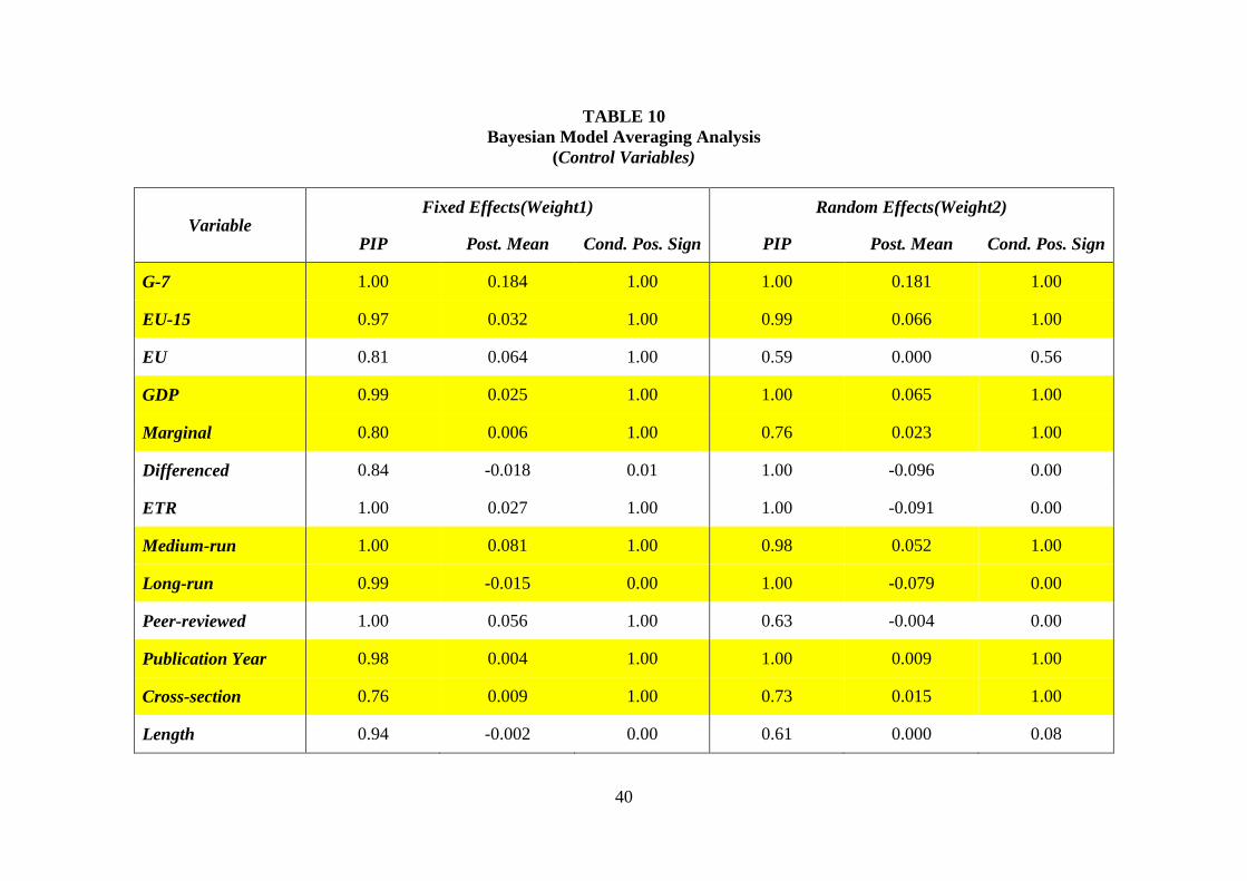
40

TABLE 10 Bayesian Model Averaging Analysis

(Control Variables)

Variable Fixed Effects(Weight1) Random Effects(Weight2)

PIP Post. Mean Cond. Pos. Sign PIP Post. Mean Cond. Pos. Sign

G-7 1.00 0.184 1.00 1.00 0.181 1.00

EU-15 0.97 0.032 1.00 0.99 0.066 1.00

EU 0.81 0.064 1.00 0.59 0.000 0.56

GDP 0.99 0.025 1.00 1.00 0.065 1.00

Marginal 0.80 0.006 1.00 0.76 0.023 1.00

Differenced 0.84 -0.018 0.01 1.00 -0.096 0.00

ETR 1.00 0.027 1.00 1.00 -0.091 0.00

Medium-run 1.00 0.081 1.00 0.98 0.052 1.00

Long-run 0.99 -0.015 0.00 1.00 -0.079 0.00

Peer-reviewed 1.00 0.056 1.00 0.63 -0.004 0.00

Publication Year 0.98 0.004 1.00 1.00 0.009 1.00

Cross-section 0.76 0.009 1.00 0.73 0.015 1.00

Length 0.94 -0.002 0.00 0.61 0.000 0.08

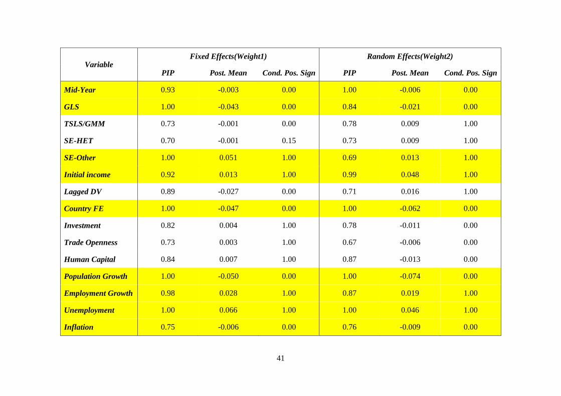
41

Variable Fixed Effects(Weight1) Random Effects(Weight2)

PIP Post. Mean Cond. Pos. Sign PIP Post. Mean Cond. Pos. Sign

Mid-Year 0.93 -0.003 0.00 1.00 -0.006 0.00

GLS 1.00 -0.043 0.00 0.84 -0.021 0.00

TSLS/GMM 0.73 -0.001 0.00 0.78 0.009 1.00

SE-HET 0.70 -0.001 0.15 0.73 0.009 1.00

SE-Other 1.00 0.051 1.00 0.69 0.013 1.00

Initial income 0.92 0.013 1.00 0.99 0.048 1.00

Lagged DV 0.89 -0.027 0.00 0.71 0.016 1.00

Country FE 1.00 -0.047 0.00 1.00 -0.062 0.00

Investment 0.82 0.004 1.00 0.78 -0.011 0.00

Trade Openness 0.73 0.003 1.00 0.67 -0.006 0.00

Human Capital 0.84 0.007 1.00 0.87 -0.013 0.00

Population Growth 1.00 -0.050 0.00 1.00 -0.074 0.00

Employment Growth 0.98 0.028 1.00 0.87 0.019 1.00

Unemployment 1.00 0.066 1.00 1.00 0.046 1.00

Inflation 0.75 -0.006 0.00 0.76 -0.009 0.00

42

NOTE: The column headings PIP, Post. Mean, and Cond. Pos. Sign stand for Posterior Inclusion Probability, Posterior Mean, and the likelihood-weighted probability that the respective coefficient takes a positive sign. These are described in the “Bayesian model averaging of control variables” subsection of Section IV in the text. The Bayesian Model Averaging (BMA) analysis was done using the R package BMS, described in Zeugner (2011). The WLS estimators Fixed Effects-Weight1 and Random Effects-Weight2 are described in the “FAT/PET tests” subsection of Section IV. All specifications included the tax variables Prediction_Negative and Prediction_Positive, which were forced into all model specifications, and adjusted for publication bias. The table yellow-highlights all the control variables that (i) have a PIP greater than 50%; (ii) have a Conditional Positive Sign of either 1.00 or 0.00 – indicating that the respective coefficient is consistently estimated to be either positive or negative in the most likely specifications; and (iii) have the same Conditional Positive Sign value for both the Fixed Effects(Weight1) and Random Effects(Weight2) estimators.

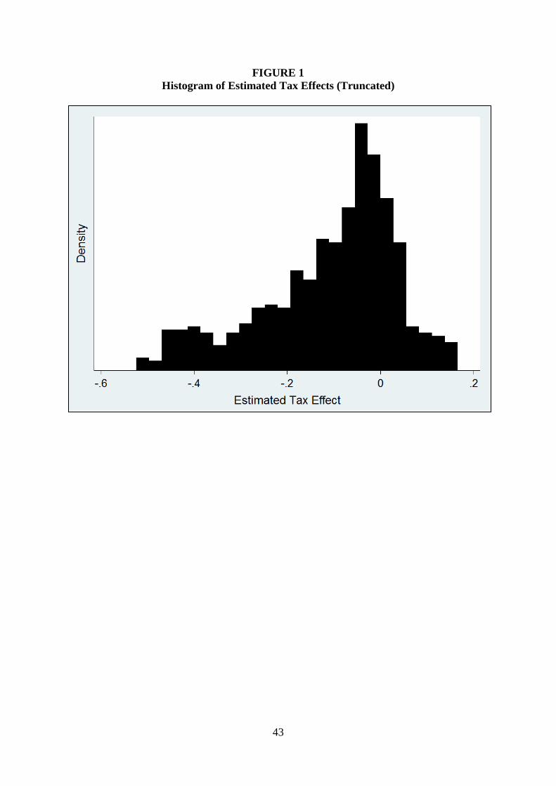
43

FIGURE 1 Histogram of Estimated Tax Effects (Truncated)

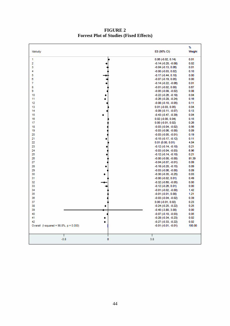
44

FIGURE 2 Forrest Plot of Studies (Fixed Effects)

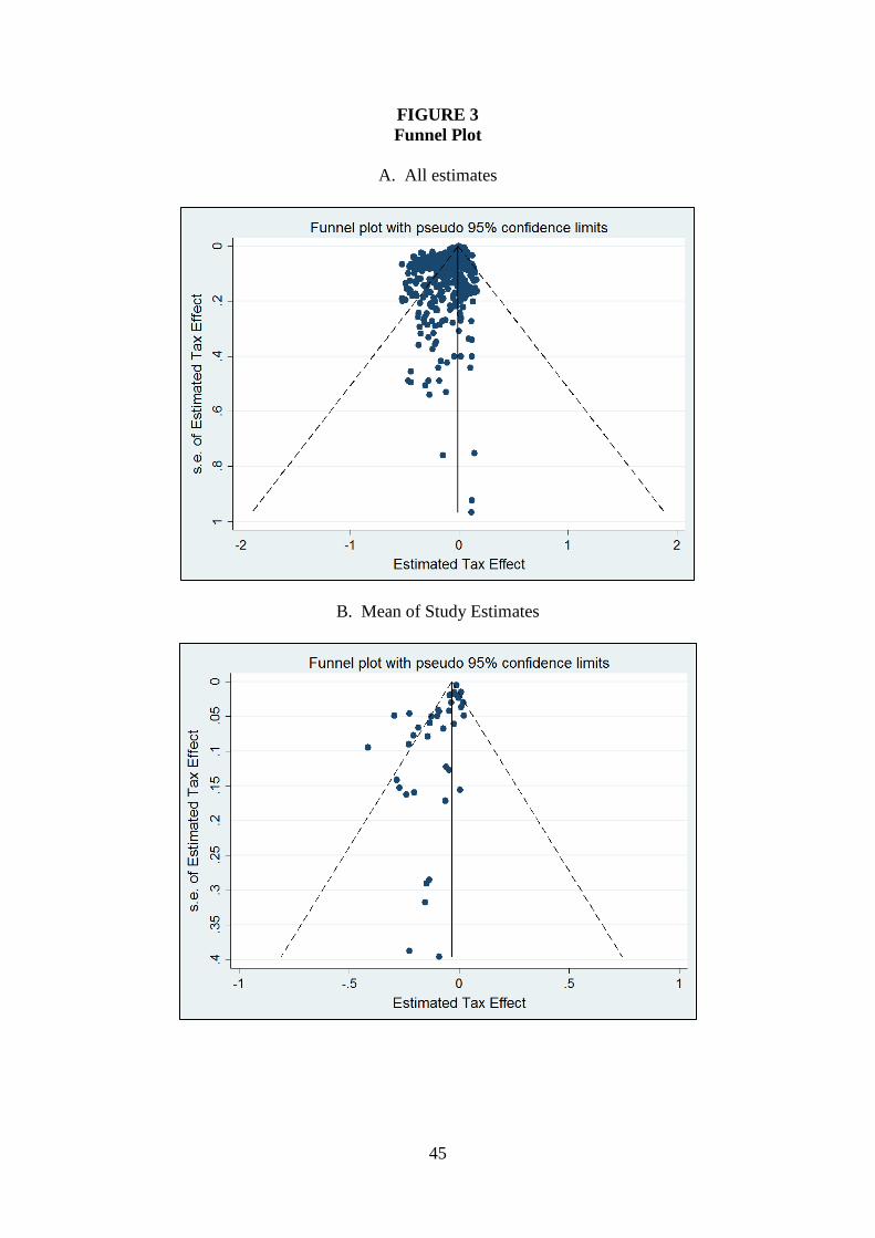
45

FIGURE 3 Funnel Plot

A. All estimates

B. Mean of Study Estimates

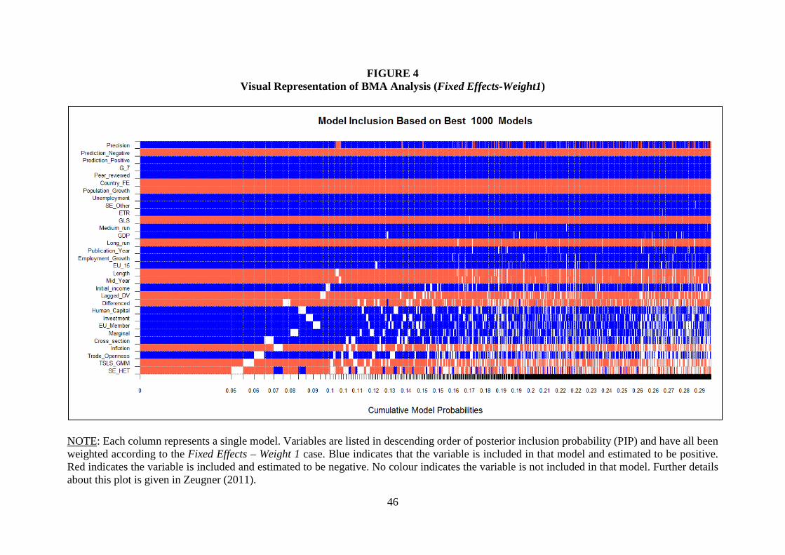
46

FIGURE 4 Visual Representation of BMA Analysis (Fixed Effects-Weight1)

NOTE: Each column represents a single model. Variables are listed in descending order of posterior inclusion probability (PIP) and have all been weighted according to the Fixed Effects – Weight 1 case. Blue indicates that the variable is included in that model and estimated to be positive. Red indicates the variable is included and estimated to be negative. No colour indicates the variable is not included in that model. Further details about this plot is given in Zeugner (2011).

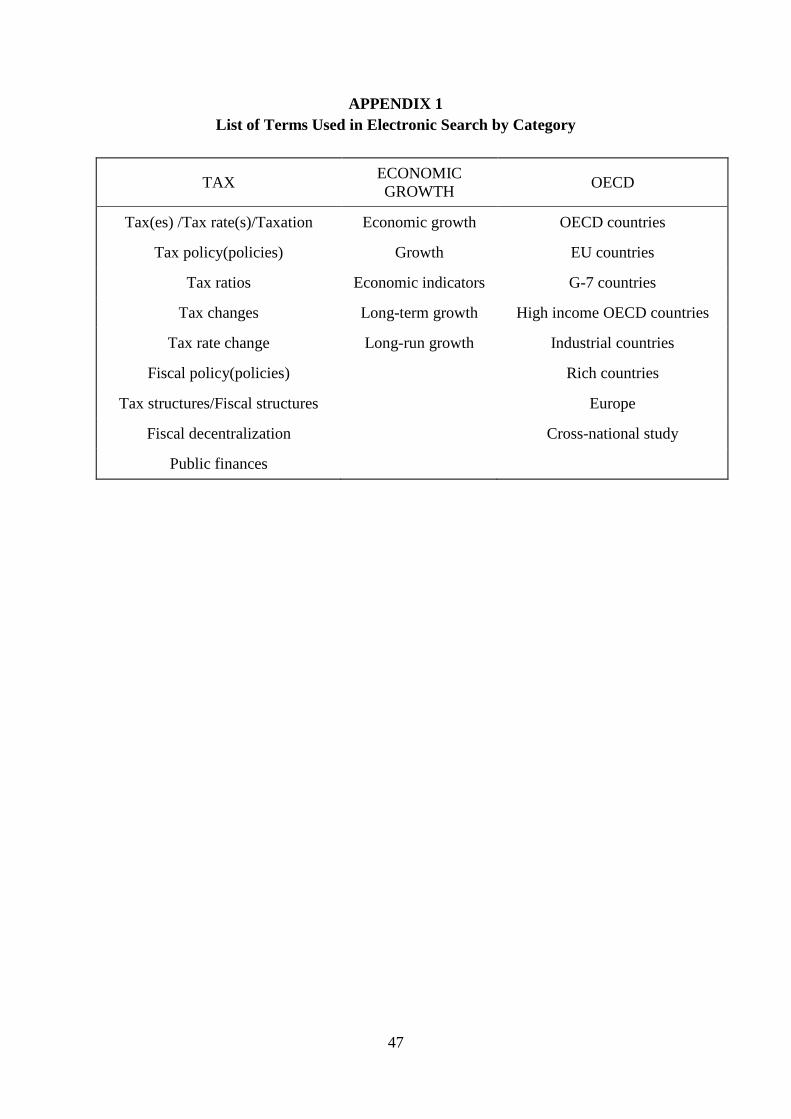
47

APPENDIX 1 List of Terms Used in Electronic Search by Category

TAX ECONOMIC GROWTH OECD

Tax(es) /Tax rate(s)/Taxation Economic growth OECD countries

Tax policy(policies) Growth EU countries

Tax ratios Economic indicators G-7 countries

Tax changes Long-term growth High income OECD countries

Tax rate change Long-run growth Industrial countries

Fiscal policy(policies) Rich countries

Tax structures/Fiscal structures Europe

Fiscal decentralization Cross-national study

Public finances

48

APPENDIX 2 Studies

ID Study Publication Status Number of estimates

1 Afonso and Alegre (2008, 2011) Working Paper + Journal 12 2 Afonso and Furceri (2010) Journal 6 3 Afonso and Jalles (2013, 2014) Working Paper + Journal 21 4 Agell et al. (1997) Journal 3 5 Agell et al. (1999) Journal 4 6 Agell et al. (2006) Journal 4 7 Alesina and Ardagna (2010) Journal 26 8 Angelopoulos et al. (2007) Journal 36 9 Arin (2004) Working Paper 80 10 Arnold et al. (2011) Journal 5 11 Arnold (2008) Working Paper 18 12 Baskaran and Feld (2013) Journal 12 13 Bergh and Karlsson (2010) Journal 3 14 Bergh and Ohrn (2011) Working Paper 10 15 Bleaney et al. (2001) Journal 19 16 Colombier (2009) Journal 13 17 Daveri et al. (1997, 2000) Working Paper + Journal 6 18 De La Fuente (1997) Discussion Paper 15 19 Folster and Henkerson (2001) Journal 7 20 Folster and Henkerson (1999) Journal 7 21 Furceri and Karras (2009) Working Paper 43 22 Gemmell et al. (2015) Journal 10 23 Gemmell et al. (2008) Working Paper 18 24 Gemmell et al. (2014) Journal 53 25 Gemmell et al. (2011) Journal 19 26 Hansson (2010) Journal 23 27 Heitger (1993) Journal 2 28 Karras and Furceri (2009) Journal 32 29 Karras (1999) Journal 28 30 Kneller et al. (1999) Journal 35 31 Mendoza et al. (1997) Journal 11 32 Miller and Russek (1997) Journal 12 33 Muinelo-Gallo and Roca-Sagales (2013) Journal 6 34 Padovano and Galli (2001) Journal 2 35 Romero-Avila and Strauch (2008) Journal 15 36 Volkerink et al. (2002) Journal 26 37 Widmalm (2001) Journal 6 38 Xing (2011) Working Paper 34 39 Abd Hakim et al. (2013) Conference Paper 2 40 Arin et al. (2015) Working Paper 6 41 Paparas et al. (2015) Journal 16 42 Xing (2012) Journal 7

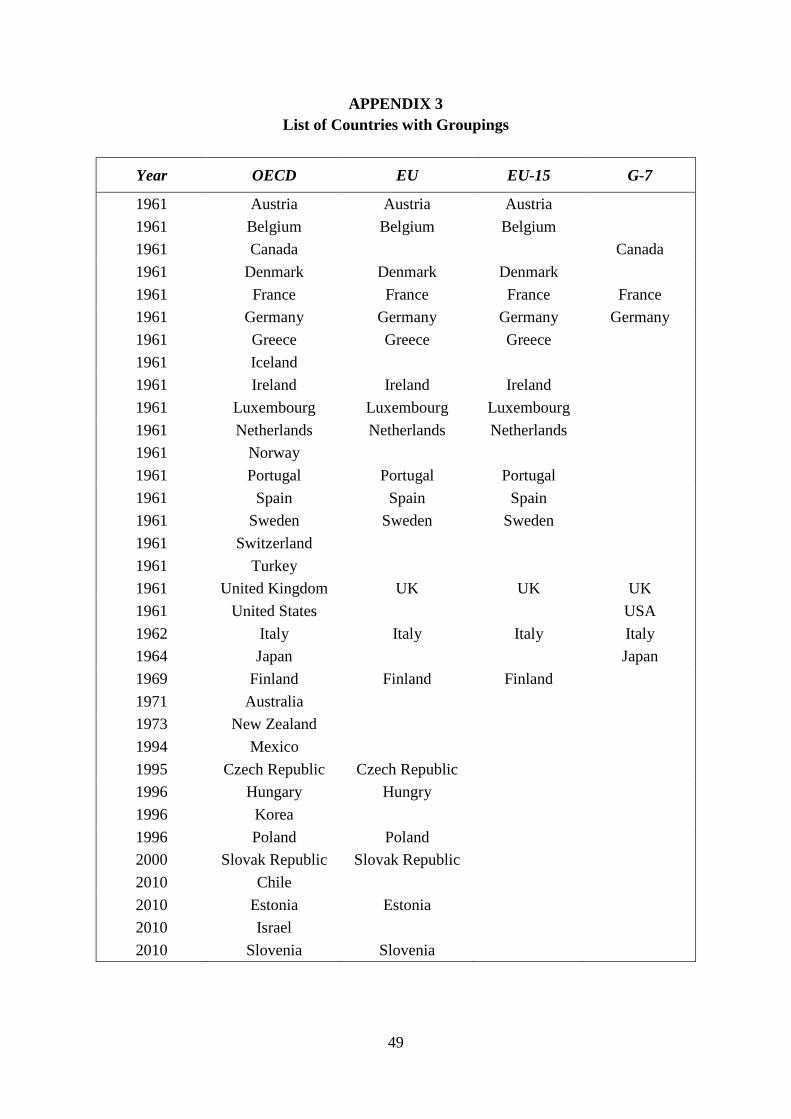
49

APPENDIX 3 List of Countries with Groupings

Year OECD EU EU-15 G-7

1961 Austria Austria Austria 1961 Belgium Belgium Belgium 1961 Canada Canada 1961 Denmark Denmark Denmark 1961 France France France France 1961 Germany Germany Germany Germany 1961 Greece Greece Greece 1961 Iceland 1961 Ireland Ireland Ireland 1961 Luxembourg Luxembourg Luxembourg 1961 Netherlands Netherlands Netherlands 1961 Norway 1961 Portugal Portugal Portugal 1961 Spain Spain Spain 1961 Sweden Sweden Sweden 1961 Switzerland 1961 Turkey 1961 United Kingdom UK UK UK 1961 United States USA 1962 Italy Italy Italy Italy 1964 Japan Japan 1969 Finland Finland Finland 1971 Australia 1973 New Zealand 1994 Mexico 1995 Czech Republic Czech Republic 1996 Hungary Hungry 1996 Korea 1996 Poland Poland 2000 Slovak Republic Slovak Republic 2010 Chile 2010 Estonia Estonia 2010 Israel 2010 Slovenia Slovenia

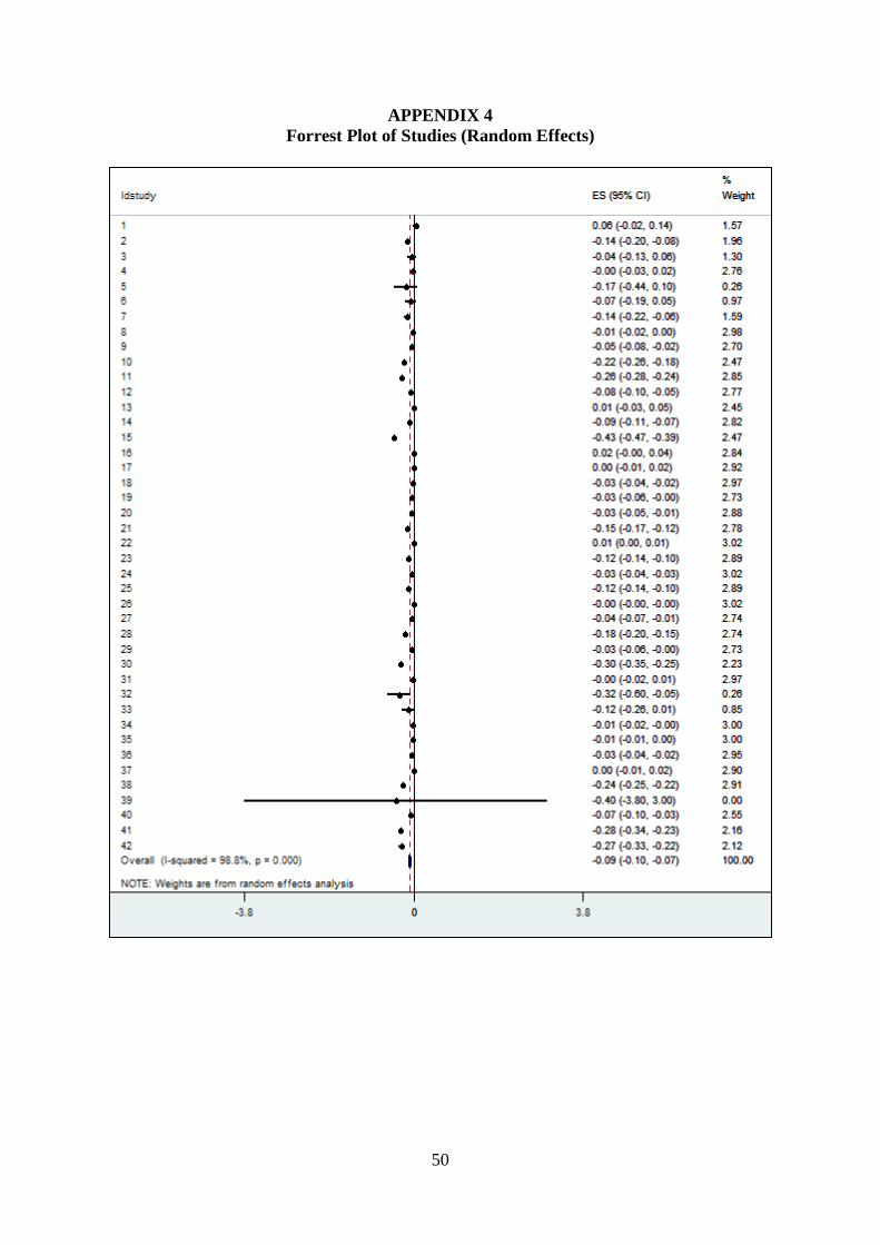
50

APPENDIX 4 Forrest Plot of Studies (Random Effects)

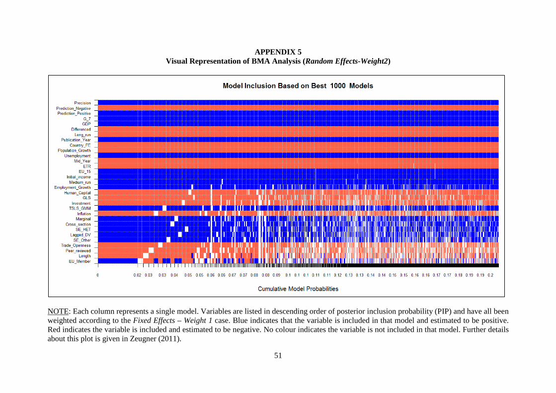
51

APPENDIX 5 Visual Representation of BMA Analysis (Random Effects-Weight2)

NOTE: Each column represents a single model. Variables are listed in descending order of posterior inclusion probability (PIP) and have all been weighted according to the Fixed Effects – Weight 1 case. Blue indicates that the variable is included in that model and estimated to be positive. Red indicates the variable is included and estimated to be negative. No colour indicates the variable is not included in that model. Further details about this plot is given in Zeugner (2011).