1

Manual

MBPAC 2012-4A

Hannah Leverentz, Erin E. Dahlke, Hai Lin, Bo Wang, Jeremy O. B. Tempkin, Helena Qi, and Donald G. Truhlar Department of Chemistry and Supercomputing Institute, University of Minnesota,

Minneapolis, MN 55455-0431

Program Version: 2012-4A

Program Version Date: September 27, 2012

Manual Version Date: October 1, 2012

Copyright 2007 – 2012

Abstract: MBPAC is a computer program for calculating electronic energies, gradients,

and/or Hessians of molecular clusters by the electrostatically embedded many-body

method (EE-MB). This program can carry out a two-body or three-body many-body

expansion for the cluster of interest, it can perform the many-body expansion on the

whole energy or just on the correlation energy, and it can use either point charges or

screened charges for the electrostatic embedding. The program works in conjunction with

either Gaussian 09 (for all types of calculations) or Molpro (for single-point energy

calculations), which is called by a script to generate the needed electronic structure data.

The code is fully parallel in that all monomer, dimer, and trimer calculations (and the full

Hartree–Fock calculation if the EE-MB-CE option has been selected) can be run

simultaneously.

2

Table of Contents

TITLE PAGE AND ABSTRACT....................................................................................1

TABLE OF CONTENTS ................................................................................................ 2

1. INTRODUCTION.......................................................................................................6

2. REFERENCES FOR MBPAC PROGRAM.................................................................8

3. GENERAL PROGRAM DESCRIPTION....................................................................9

4. THEORETICAL BACKGROUND ...........................................................................11

4.A. MANY-BODY EXPANSION....................................................................... 11

4.B. ELECTROSTATICALLY EMBEDDED MANY-BODY EXPANSION WITH POINT CHARGES................................................................................................ 12

4.C. SCREENED CHARGE MODEL.................................................................... 15

4.D. ELECTROSTATICALLY EMBEDDED MANY-BODY EXPANSION OF THE CORRELATION ENERGY........................................................................... 17

5. INSTALLING MBPAC ............................................................................................19

5.A. INSTALLATION INSTRUCTIONS ................................................................ 19

6. DESCRIPTION OF FILES IN MBPAC ....................................................................24

6.A. SOURCE CODE........................................................................................ 24

6.A.1. SERIAL SOURCE CODE FILES........................................................ 24

6.A.2. SUBPROGRAM LIST ...................................................................... 26

6.A.3. PARALLEL SOURCE CODE FILES ................................................... 37

6.A.4. PARALLEL SUBPROGRAM LIST ..................................................... 38

6.B. FILES REQUIRED TO RUN MBPAC............................................................. 39

6.B.1. G09SHUTTLE.PL SCRIPT ............................................................... 39

6.B.2. MOLPSHUTTLE.PL SCRIPT............................................................. 40

6.B.3. EX_SHUTTLE, G09-EX-SHUTTLE, AND GAU_EXTERNAL_2 SCRIPTS40

6.C. FILES CREATED DURING ALL MBPAC RUNS ............................................. 41

3

6.C.1. THE OUTPUT FILE........................................................................ 41

6.C.2 THE X_Y.EEMB FILES ..................................................................... 42

6.C.3 THE FULLHF_1.TXT FILE ............................................................... 43

6.D. FILES CREATED ONLY DURING GAUSSIAN RUNS..................................... 43

6.D.1. THE N.G09 AND MMN.G09 FILES ................................................. 43

6.D.2. THE N.OUT AND MMN.OUT FILES .................................................. 44

6.D.3. TEST.FCHK and MMTEST.FCHK .................................................. 44

6.D.4 ADDITIONAL FILES CREATED DURING AN EXTERNAL OPTIMIZATION.............................................................................................................. 44

6.D.5 THE MMCORRN.OUT FILE ............................................................. 44

6.E. FILES CREATED ONLY DURING MOLPRO RUNS........................................ 45

6.E.1. THE N.INP AND N.LAT FILES ......................................................... 45

6.E.2. THE N.OUT AND N.XML FILES........................................................ 45

7. USING MBPAC........................................................................................................46

7.A. THE PERL SCRIPT EEMB.PL...................................................................... 46

7.B. THE RESTART OPTION ............................................................................ 47

8. INPUT FILE STRUCTURE AND EXPLANATION OF INPUT VARIABLES........48

8.A. GENERAL SECTION .............................................................................. 49

8.B. FRAGMENT SECTION ........................................................................... 51

8.C. JOB SECTION.......................................................................................... 53

9. THE MBPAC TEST SUITE......................................................................................60

9.A. INTRODUCTION TO THE TEST SUITE......................................................... 60

9.B. THE TEST RUNS...................................................................................... 60

9.B.1. TEST 1......................................................................................... 60

9.B.2. TEST 2......................................................................................... 60

4

9.B.3. TEST 3......................................................................................... 61

9.B.4. TEST 4......................................................................................... 62

9.B.5. TEST 5......................................................................................... 62

9.B.6. TEST 6......................................................................................... 62

9.B.7. TEST 7......................................................................................... 62

9.B.8. TEST 8......................................................................................... 63

9.B.9. TEST 9......................................................................................... 63

9.B.10. TEST 10..................................................................................... 63

9.B.11. TEST 11..................................................................................... 65

9.B.12. TEST 12..................................................................................... 65

9.B.13. TEST 13..................................................................................... 65

9.B.14 TEST 14...................................................................................... 66

9.B.15 TEST 15...................................................................................... 66

9.B.16 TEST 16...................................................................................... 66

9.B.17 TEST 17...................................................................................... 67

9.B.18. TEST 18..................................................................................... 67

9.B.19. TEST 19..................................................................................... 67

9.B.20. TEST 20..................................................................................... 67

9.B.21 TEST 21...................................................................................... 67

9.B.22. TEST 22..................................................................................... 68

9.B.23. TEST 23..................................................................................... 68

9.B.24. TEST 24..................................................................................... 68

9.B.25. TEST 25..................................................................................... 69

9.B.26. TEST 26..................................................................................... 69

9.B.27. TEST 27..................................................................................... 69

5

10. COMPUTERS, OPERATING SYSTEMS, AND COMPILERS ON WHICH THE CODE WAS TESTED ..................................................................................................70

11. CITED REFERENCES ...........................................................................................76

12. BIBLIOGRAPHY ...................................................................................................78

13. REVISION HISTORY ............................................................................................79

13.A. VERSION 1.0 ........................................................................................ 79

13.B. Version 2007 ....................................................................................... 79

13.C. Version 2007-2.................................................................................... 79

13.D. Version 2009 (May 28, 2009) .............................................................. 79

13.E. Version 2009-2 (June 25, 2009) ........................................................... 80

13.F. Version 2011 (March 18, 2011)............................................................ 81

13.G. Version 2011-2 (April 13, 2011).......................................................... 82

13.H. Version 2011-3 (June 21, 2011)........................................................... 83

13.I. Version 2011-3A (July 7, 2011) ............................................................ 84

13.J. Version 2011-4 (July 13, 2011)............................................................. 85

13.K. Version 2011-5 (November 22, 2011).................................................. 85

13.L. Version 2012 (February 13, 2012)........................................................ 86

13.M. Version 2012-2 (May 16, 2012) .......................................................... 87

13.N. Version 2012-3 (May 23, 2012)........................................................... 88

13.O. Version 2012-4 (July 11, 2012) ........................................................... 88

13.P. Version 2012-4A (September 27, 2012) ............................................... 89

6

Chapter One

Introduction

MBPAC is a computer program for calculating single-point energies, gradients,

Hessians, geometry optimizations, and/or population analyses of molecular clusters using

the electrostatically embedded many-body (EE-MB) method.1 The current version

allows for energy and population analysis calculations using a two-body expansion

(EE-PA) or a three-body expansion (EE-3B). The background charges used in the

calculation are user defined, enabling one to utilize any charge model for the electrostatic

embedding. With this version of the program, calculations can be carried out using any

electronic structure method available in GAUSSIAN 092 that can be used in a two-layer

ONIOM calculation (see the keyword ONIOM in the GAUSSIAN 09 manual) or any

electronic structure method available in MOLPRO3. Any pre-defined or user-defined basis

set that is compatible with GAUSSIAN 09 or MOLPRO may be used. MBPAC 2012-4A can

treat clusters but does not yet include periodic boundary conditions.

Four kinds of calculations can be done with MBPAC 2012-4A using GAUSSIAN 09:

energies, gradients, Hessians, and geometry optimizations (which use the GAUSSIAN 09

external optimizer). MOLPRO can be used only for energy calculations. The list below

indicates the order in which each of the GAUSSIAN 09 calculations will be done within the

program. If the user has not selected one of these calculations then the program will go

on to the next calculation in the list.

1. External optimization. The MBPAC 2012-4A program has been interfaced with

the external optimizer in the GAUSSIAN 09 software package. This is currently

7

the only means for geometry optimization. No restart option is currently

implemented for geometry optimizations.

2. Hessian calculation. Frequencies and normal mode coordinates are also

calculated in the Hessian calculation by mass-scaling and diagonalizing the

Hessian matrix.

3. Gradient calculation. The gradient calculation is carried out only if a Hessian

was not calculated since a Hessian calculation outputs both a gradient and an

energy.

4. Energy calculation. An energy calculation is carried out only if a Hessian or

gradient calculation was not done because both of these calculations output an

energy as well.

Chapter 2 gives the references for the MBPAC program in three different styles,

and Chapter 3 gives a general program description. Chapter 4 presents the theoretical

background of the EE-PA and EE-3B methods, Chapter 5 describes the installation, and

Chapter 6 provides a complete listing of all the files that comprise the MBPAC package.

Chapter 7 discusses how to use the MBPAC program, Chapter 8 discusses the structure of

the input file, Chapter 9 presents the test jobs, and Chapter 10 describes the computers,

operating systems, and compilers the code has been tested on. Chapter 11 gives the cited

references, Chapter 12 gives a bibliography of all published papers from our group

pertaining to the EE-MB method, and Chapter 13 gives the revision history.

8

Chapter Two

References for MBPAC Program

The recommended reference for the current version of the code is given below in

three styles, J. Chem. Phys. style, J. Amer. Chem. Soc. style, and Chem. Phys. Lett. style.

J. Chem. Phys. style:

H. Leverentz, E. E. Dahlke, H. Lin, B. Wang, J. O. B. Tempkin, H. W. Qi, and D. G.

Truhlar, MBPAC 2012-4A (University of Minnesota, Minneapolis, 2012).

J. Amer. Chem. Soc. style:

Leverentz, H.; Dahlke, E. E.; Lin, H.; Wang, B; Tempkin, J. O. B.; Qi, H. W.; Truhlar, D.

G. MBPAC 2012-4A, University of Minnesota, Minneapolis, 2012.

Chem. Phys. Lett. style:

H. Leverentz, E.E. Dahlke, H. Lin, B. Wang, J.O.B. Tempkin, H.W. Qi, D.G. Truhlar,

MBPAC 2012-4A. University of Minnesota, Minneapolis, 2012.

The user should also reference the GAUSSIAN 09 electronic structure program (see

Reference 2 in Chapter 11) or the MOLPRO 2010 electronic structure program (see

Reference 3 in Chapter 11) .

9

Chapter Three

General Program Description

MBPAC is written in FORTRAN77 and uses a PERL script to interface with

GAUSSIAN 09 or MOLPRO 2010. The program is written using modular subprograms

called “hooks”. There are four main hooks: energy hook (ehook), gradient hook

(ghooks), Hessian hook (hhook), and optimization hook (ohook). Each one of these

hooks is designed to be able to utilize a variety of electronic structure methods and basis

sets. All of the hooks interface with the GAUSSIAN 09 software program and the energy

hook also interfaces with the MOLPRO software program. The user must provide an input

file (described in Chapter 8) that provides, in addition to other information, the geometry

of the cluster, an array that identifies each atom for each fragment, and the background

charges to be used in the electrostatic embedding.

For single point energies, gradients, and Hessians MBPAC uses the information

provided in the input file to break the cluster up into all possible fragment combinations

for the EE-MB calculation requested and write the corresponding GAUSSIAN 09 or

MOLPRO input files. When the input file is complete the g09shuttle or molpshuttle script

is called to run the GAUSSIAN 09 or MOLPRO calculation, parse the required data, and

place it into a file. When all electronic structure calculations are finished, the MBPAC

program extracts all of the data from the file and calculates the EE-PA or EE-3B energy.

The overall control of the program is:

MBPAC ↔ g09shuttle/molpshuttle ↔ GAUSSIAN 09/ MOLPRO ↔ g09shuttle/molpshuttle

↔ MBPAC

10

Geometry optimizations are carried out using the external optimizer of

GAUSSIAN 09. The overall control for this procedure is:

MBPAC ↔ g09shuttle ↔ GAUSSIAN 09 ↔ Gau_External_2 ↔ g09shuttle ↔ MBPAC

If one chooses to do a geometry optimization the primary MBPAC calculations will call a

GAUSSIAN 09 optimization with the external keyrword. This GAUSSIAN 09 calculation

calls an external PERL script Gau_External_2, which will provide the MBPAC energy and

gradient needed for optimization. Gau_External_2 will call a secondary MBPAC

calculation and pass the results to GAUSSIAN 09. When GAUSSIAN 09 finishes the

optimization, it will return the optimized geometry to the primary MBPAC calculations.

The optimized geometry will be printed along with the energy and gradient.

11

Chapter Four

Theoretical Background

This chapter describes the EE-MB method.

4.A. MANY-BODY EXPANSION

For a system containing N particles the total energy of the system can be written,

without any approximation, as:4

V = V1 + V2 + V3 + + VN (1)

where

V1 = Ei

i

N

! (2)

V2 = (Eij ! Ei ! E j )i< j

N" (3)

V3 = [(Eijk !i< j<k

N" Ei ! E j ! Ek) ! (Eij ! Ei ! E j ) ! (Eik ! Ei ! Ek) ! (E jk ! E j ! Ek)](4)

and so on for higher order terms, where Ei, Eij, Eijk, … are the energies of a monomer,

dimer, trimer, and so forth. In general it is assumed that the series in equation 1

converges rapidly, and in general only the first few terms are kept. If only the first and

second terms of equation 1 are kept, the total energy becomes

EPA = Eij ! (N ! 2)i< j

N" Ei

i

N" (5)

12

and one is said to have made the pairwise additive (PA) approximation. If one keeps the

first three terms of equation 1, one is said to have made the three-body approximation

(3B), and the total energy can be written as :

E3B = Eijk ! (N ! 3)i< j<k

N" Eij +

(N !2)(N ! 3)

2i< j

N" Ei

i

N" (6)

In general the pairwise additive approximation is accurate enough to determine

qualitative trends, however, if one is interested in quantitative accuracy, inclusion of

higher-order terms is necessary.4 For a system in which the many-body terms are large

one may need to include several of the higher-order terms in order to obtain the desired

accuracy.

4.B. ELECTROSTATICALLY EMBEDDED MANY-BODY EXPANSION WITH POINT CHARGES

In order to speed up the convergence of equation 1, one can embed each n-body

cluster in a field representing the other N – n atoms. In the electrostatically embedded

many-body expansion, with the point charge option (the screened charge option is

discussed in Section 4.C), this is done by placing atom-centered point charges at the

positions of the atoms in the other N – n fragments. When this is done equations 2 – 4

can be rewritten as

V1 = Ei'

i

N

! (7)

V2 = (Eij' ! Ei

' ! E j' )

i< j

N" (8)

and

V3 = [(Eijk' !

i< j<k

N" Ei

' ! E j' ! Ek

' ) ! (Eij' ! Ei

' ! E j' ) ! (Eik

' ! Ei' ! Ek

' ) ! (E jk' ! E j

' ! Ek' )](9)

13

where the prime denotes the energy of an embedded fragment. By an embedded

fragment we mean the fragment embedded in the field of point charges as described

above.

The electrostatically embedded pairwise additive (EE-PA) and electrostatically

embedded three-body (EE-3B) energies are defined analogously to equations 5 and 6 as

EEE -PA = Eij' ! (N !2)

i< j

N" Ei

'

i

N" (10)

and

EEE -3B = Eijk' ! (N ! 3)

i< j<k

N" Eij

' +(N !2)(N ! 3)

2i< j

N" Ei

'

i

N" (11)

where the primes in equations 10 – 11 have the same meaning as in 7 – 9. The term

EE-MB denotes an electrostatically embedded many-body expansion of unspecified

order.

If electrostatic embedding is carried out to Nth order (i.e., EE-NB), where N is

equal to the number of fragments in the whole cluster, one will get the exact result. This

result will be independent of the choice of charge model used and will give the same

results with or without embedding if equation 1 is used without truncation. However it

has been shown5 that the rate of the convergence for the series (i.e., the accuracy if one

truncates after a given order of many-body terms) depends strongly on embedding.

One can also use a similar expansion to determine the MB or EE-MB

approximation of the components of the full-system dipole moment:

µ!EE-PA =

j"i

# µ!ij $ N $2( )µ!

i

(12)

14

µ!EE-3B

=

j"i

N

#k"ik> j

N

# µ!ijk$ N $ 3( )

j"i

N

# µ!ij

+N $ 2( ) N $ 3( )

2µ!i

(13)

In eqs 12 and 13,

µ!EE-MB

is the EE-MB approximation to the ν-component of the dipole

moment, where ν can be replaced by x, y, or z. The expressions

µ!ijk

,

µ!ij

, and

µ!i

are the

ν-component of the dipole resulting from the wave functions or electron densities of

trimer ijk, dimer ij, and monomer i, respectively.

Similarly, one may find the MB or EE-MB approximation of the full-system

partial charge distribution that would result from various types of population or charge

analysis, such as Mulliken6 or CHelpG7:

qAEE-PA =

j!i

" qAij# N # 2( )qA

i

(14)

qAEE-3B

=

j!i

N

"k!ik> j

N

" qAijk# N # 3( )

j!i

N

" qAij

+N # 2( ) N # 3( )

2qAi

(15)

In eqs 14 and 15,

qAEE-MB

is the EE-MB partial charge assigned to atom A belonging to

monomer i, and

qAijk

,

qAij

, and

qAi

are the partial charges assigned to atom A by the

population or charge analyses of the wave functions or electron densities of trimer ijk,

dimer ij, and monomer i, respectively.

There are several different ways in which the background point charges to be used

in the embedding can be chosen. Three possible ways to determine the background point

charges are:

15

A. Determine a charge representation for the entire cluster; then, for each monomer,

dimer, or trimer, represent the other N – 1, N – 2, or N – 3 fragments with the

charges from this full-system charge calculation.

B. For each monomer present in the cluster, determine a charge respresentation for

the monomer in the same geometry that it has in the cluster, and then for each

monomer, dimer, or trimer, represent the other N – 1, N – 2, or N – 3 fragments

with the charges from these monomer calculations.

C. For each type of molecule present in the cluster determine a charge representation

for the geometrically relaxed gas-phase monomer, and then for each monomer,

dimer, or trimer, represent the other N – 1, N – 2, or N – 3 fragments with the

charges from these monomer calculations.

One can see that for a very large cluster the use of charge models A and B could prove to

be expensive and time consuming, and it has been shown that for water clusters, which

are known to have large many-body effects8 (and thus slow convergence of equation 1),

the use of strategy C gives sufficient accuracy to give good quantitative results.5

Another important choice is which charge representation to use (e.g., Mulliken,6

Löwdin,9, 10 redistributed Löwdin,11 CM4,12 or force field). The optimal set of charges

may be different for each system, and it is up to the user to choose a set of charges that

meets his or her desired accuracy level.

4.C. SCREENED CHARGE MODEL

Background charges can also be represented by screened charges16 rather than

point charges. The screened charge scheme improves the point charge scheme by taking

into account the penetration effects. The charge density of an atom is represented by two

16

components: (i) a smeared charge, of magnitude

!nscreen , distributed like electrons in the

orbital

! (n) = Arn"1 exp("#r) , which models the extension of the MM electron density

and (ii) the rest of the charge, which is located at the nucleus. The comparison of a point

charge model and a screened charge model is shown in Figure 1. Note that this screening

procedure is sometimes called outer density screening (ODS) to distinguish it from other

screening models.

Figure 1. Comparison between (a) a point charge model and (b) a screened charge model

of an MM atom A. The total smeared charge in model (b) is

!nscreen , representing

nscreen electrons.

Based on the new model, we can calculate the effective charge of the atom A as

qA*

= qA + nscreen f (!r)exp("2!r) (16)

where the scaling factor f is

f (!r) =1+ !r n =1

=1+3

2!r + (!r)2 +

1

3(!r)3 n = 2

=1+5

3!r +

4

3(!r)2 +

2

3(!r)3 +

2

9(!r)4 +

2

45(!r)5 n = 3

=1+7

4!r +

3

2(!r)2 +

5

6(!r)3 +

1

3(!r)4 +

1

10(!r)5 +

1

45(!r)6 +

1

315(!r)7 n = 4

(17)

17

In the screened charge model of eq. (16), the effective charge has two terms: the

conventional point charge and an addition term to include the penetration effects. The

latter term goes to zero when r approaches infinity and goes to qA+nscreen when r

approaches 0. The parameters of

! for common atoms (H, C, N, O, F, Si, P, S, Cl and Br)

have been optimized and they have been listed in the Table 1.

Table 1. ζ values used in the Slater-type orbital

Atom H B C N O F Si optimized parameters 1.32 0.92 0.92 1.20 1.16 0.73 MSB parametersa 1.32 0.72 0.87 1.01 1.12 1.24 0.74

Atom P S Cl Ge As Se Br optimized parameters 0.68 0.90 0.98 0.91

MSB parametersa 0.81 0.88 0.95 0.83 0.88 0.95 1.01

a modified Strand-Bonham (MSB) parameters (optimized parameter for H and half of the

Strand-Bonham parameters for B through Br)

4.D. ELECTROSTATICALLY EMBEDDED MANY-BODY EXPANSION OF THE CORRELATION ENERGY

If one is using a post-Hartree–Fock level of wave function theory such as MP2,

QCISD(T), or CCSD(T), one can define the system’s correlation energy (

!

"Vcorr ) as the

energy at the higher level of electronic structure theory (V) minus the Hartree–Fock

energy (

!

VHF

) using the same basis set; that is,

!

"Vcorr =V #VHF

. One can then expand

the correlation energy in exactly the same way that one expands the total energy in the

MB or EE-MB approximations in equations 1–4 or 7–9:

!

"Vcorr = "Vcorr(1)

+ "Vcorr(2)

+ "Vcorr(3)

+ ...+ "Vcorr(N ) (18)

where, for example,

18

!

"Vcorr(2) = "Eij

corr #"Eicorr #"E j

corr( )i< j

N

$ (19)

and, for example,

!

"Eijcorr

= Eij # EijHF (20)

with

!

Eij being the energy of dimer ij at the post-Hartree–Fock level of wave function

theory (electrostatically embedded in any chosen manner) and with

!

EijHF being the

energy of dimer ij at the Hartree–Fock level of wave function theory.

One can then approximate the total energy of the system as the sum of the

Hartree–Fock energy of the entire system with any desired number of terms in the

expansion of the correlation energy. When one has done this, one has made the EE-MB-

CE approximation to the total energy of the system. The EE-PA-CE energy is written as

!

VEE-PA-CE

=VHF

+ "Vcorr(1)

+ "Vcorr(2) (21)

and the EE-3B-CE energy is written as

!

VEE-3B-CE

=VHF

+ "Vcorr(1)

+ "Vcorr(2)

+ "Vcorr(3) (22)

Although these methods scale roughly as N4 with system size due to the need for a full-

system Hartree–Fock calculation, this is still a much more favorable scaling than any of

the post-Hartree–Fock levels of theory, and it can yield results that are within 1 kcal/mol

of the conventional calculations.17

19

Chapter Five

Installing MBPAC

A step-by-step procedure for installing MBPAC on a Unix computer is given here.

Compilation of the MBPAC program can be accomplished with the PERL script configure.

The test runs described in Chapter 8 illustrate the proper way in which to use the

program.

5.A. INSTALLATION INSTRUCTIONS

Step 1:

The MBPAC program should have been obtained in the tar format with the following

name: mbpac2012-4A.tar.gz. This file should be placed in the directory in which the user

wishes to install MBPAC, and then the following two commands should be executed:

gunzip mbpac2012-4A.tar.gz

tar –xvf mbpac2012-4A.tar

Once these two commands have been executed the directory structure in the next step

should have been created. Please make sure that this is true.

Step 2:

Verify that the files have been placed into the directory structure as follows.

In the mbpac2012-4A directory

basis/ configure exe/ psrc/

script/ src/ testo/ testrun/

20

In the basis directory:

mg3s.gbs b2.gbs acTZ_noHe.gbs

631+gdp_noHe.gbs JUN-cc-pVTdZ.mbs

The exe directory should be empty.

In the psrc directory:

common.inc eehed.f ehooks.f frag.f

freq.f ghooks.f hhooks.f main.f

ohooks.f read.f worker.f

In the script directory:

checktestrun check_all.pl clean.pl eemb.pl

ex_shuttle g09shuttle.pl g09-ex-shuttle.pl Gau_External_2

mbcompile molpshuttle.pl testall.pl updatetesto

updatetestrun

In the src directory:

common.inc eehed.f ehooks.f frag.f

freq.f ghooks.f hhooks.f main.f

ohooks.f read.f

In the testrun directory:

test1/ test2/ test3/

test4/ test5/ test6/

test7/ test8/ test9/

test10/ test11/ test12/

test13/ test14/ test15/

21

test16/ test17/ test18/

test19/ test20/ test21/

test22/ test23/ test24/

test25/ test26/ test27/

In each of the testrun/testn directories (where n is the number of the test run) :

eemb.pl testn.inp

Test run 7 illustrates the restart option (see section 8.B.) and the test7

directory contains the following additional files:

x_1.eemb y_2.eemb

where x = 1, 2, 3, and 4 and where y = 1, 3, 4, 5, and 6. Please see section

8.A.7 for more information.

In the testo directory:

test1/ test2/ test3/

test4/ test5/ test6/

test7/ test8/ test9/

test10/ test11/ test12/

test13/ test14/ test15/

test16/ test17/ test18/

test19/ test20/ test21/

test22/ test23/ test24/

test25/ test26/ test27/

In each of the testo/testn directories (where n is the number of the test run):

testn.out

22

Step 3:

Change the working directory to the mbpac2012-4A directory, and run the script

configure by typing:

./configure<Return>

This script will create a file in your home directory named .mbpac_path stating where the

MBPAC directory structure is located. This file is used by other scripts to locate MBPAC on

the user’s system. The configure script will look for one of the following serial

compilers: g77, xlf, or ifort. It will also look for one of the following MPI compilers:

mpxlf, ifort, or mpif90. If it successfully finds one of the MPI compilers it will ask if you

would like to attempt to compile the parallel version of the code (found in the psrc

directory). If you say no, or, if it is unable to find an MPI compiler, it will compile the

serial version of the code (found in the src directory). Both the parallel and serial

compilations are carried out by running the script mbcompile in the script directory.

Successful compilation of the serial version of the code will place the executable

mbpac.exe in the directory exe. Successful compilation of the parallel version of the code

will place the executable pmbac.exe in the exe directory.

If the configure scripts is unable to find any MPI or any serial compilers, or if

you tell it that it will ask you to manually input the name of your compiler into the first

line of the Makefile. If the user would like to compile the serial version of the code they

must edit the Makefile in the directory src as described above, and then compile by

typing:

gmake mbpac.exe<Return>

23

and manually move the executable mbpac.exe to the exe subdirectory. If the user would

like to compile the parallel version of the code they must edit the Makefile in the psrc

directory and compile by typing:

gmake pmbpac.exe<Return>

and manually move the executable pmbpac.exe to the exe subdirectory.

After compilation please check to make sure that there are five object files

(corresponding to the five source code files listed above) in the src or psrc directory, and

that there is an executable file named mbpac.exe or pmbpac.exe in the exe directory. If

any of these files are missing, something went wrong during the compilation.

Step 4:

While in the script directory, edit the variable $g09, in the g09shuttle.pl and the

g09-ex-shuttle.pl scripts, so that the path indicated for the GAUSSIAN 09 program is

accurate for the computer system on which MBPAC has been installed. Also edit the

variable $molp, in the molpshuttle.pl script, so that the path indicated for the MOLPRO

program is accurate for the computer system on which MBPAC has been installed. The

user should also change the variable $scratchdir variable that appears in both of these

scripts to the directory on his/her computer where s/he would like the GAUSSIAN 09 or

MOLPRO program to carry out its calculations and place the scratch files.

24

Chapter Six

Description of Files in MBPAC

This chapter describes the files involved in the compiling and running of MBPAC,

in particular: the source code needed to compile MBPAC, files required to run MBPAC, files

created during an MBPAC run, and a script supplied to simplify the running of MBPAC.

6.A. SOURCE CODE

The serial MBPAC source code is composed of five FORTRAN77 files. Subsection 7.A.1

describes each file in the serial source code, and 7.A.2 lists each subprogram in the serial

version of MBPAC, in alphabetical order, and describes it. Subsection 7.A.3 lists the

FORTRAN77 files for the parallel version of MBPAC that are not included in, or are

different than, the serial version, and subsection 7.A.4 lists the subprograms in these files

that are not included in, or are different than, those listed in subsection 7.A.2.

6.A.1. SERIAL SOURCE CODE FILES

common.inc

This file contains all the parameters that limit the system and fragment sizes in the

MBPAC program. The parameters defined are

MAXAT the maximum number of atoms allowed in the system

MAXAPF the maximum number of atoms allowed in a fragment

MAXFRAG the maximum number of fragments allowed in the system,

defined as MAXAT/MAXAPF

MAXE the maximum number of energies printed in the output file

25

MAXLIST the maximum number of fragment combinations that can be

calculated, defined by specifying MAXAT

MAXHESS the maximum number of Hessian elements that can be stored,

defined by specifying MAXAT

eehed.f

This file contains the subprograms to write the header information and input

summary to the output file. It also contains the subprogram to set the default

variables.

ehooks.f

This file contains all of the subprogram for carrying out the energy calculations.

It also contains the subroutines for determining the restart information for energy

calculations.

frag.f

This file contains the subprograms for generating all possible fragment

combinations for a given cluster and calculation type, getting the geometry,

charge, and multiplicity for the correct fragment, and getting the correct

background charges.

freq.f

This file contains the subprograms for calculating the frequencies once the

Hessian has been computed.

ghooks.f

This file contains the subprograms for carrying out gradient calculations. It also

contains the subroutines for determining the restart information for gradient

26

calculations.

hhooks.f

This file contains the subprograms for carrying out a Hessian calculation. It also

contains the subroutines for determinging the restart information for Hessian

calculations.

main.f

This file contains the driver for the MBPAC program.

read.f

This file contains all the subprograms for parsing the input file eemb.inp.

6.A.2. SUBPROGRAM LIST

In this section the subprogram names are in bold. On the same line is the type of

subprogram and the file it is in. The following lines list what subprograms call it and a

short description of the subprogram.

atomic function ehooks.f

called by: eg09

Converts the symbol of the atom type to its atomic number.

calcmbce subroutine ehooks.f

called by: wg09e

Calculates the requested EE-MB-CE approximation of the system’s energy.

case function read.f

called by: rline, chkln, g09outo

Converts a string to all lower case.

27

cfloat function read.f

called by: rgeom

Converts an integer to a double precision number.

chgcorr subroutine ehook.f

called by: eg09

Calculates the energy of interaction between QM nuclei and screened charges.

chgmlt subroutine frag.f

called by: eg09, gg09, hg09

Calculates the charge and multiplicity of a cluster of fragments.

chkcompat subroutine read.f

called by: readin

Checks to make sure that the type of calculation and the keywords specified by

the user are compatible with one another and generates an error message if they

are not.

chkcpop subroutine read.f

called by: eg09, rjob

Checks whether the method of population analysis selected by the user is

supported by MBPAC.

chkln subroutine read.f

called by: rline, rtitl, rline2

Checks a line to see if it's a special type.

daxpy subroutine freq.f

called by: dgefa, dgedi

28

Computes a constant times a vector plus a vector.

defalt subroutine eehed.f

called by: main

Sets the default variables for the program.

dgefa subroutine freq.f

called by:

Factors a double precision matrix by Gaussian elimination

dgedi subroutine freq.f

called by: prjfc

Computes the determinant and inverse of a matrix.

dscal subroutine freq.f

called by: dgefa, dgedi

Scales a vector by a constant.

dswap subroutine freq.f

called by: dgedi

Interchanges two vectors.

eehed subroutine eehed.f

called by: main

Writes the program header to the output file.

eg09 subroutine ehooks.f

called by: ehooks

Writes and runs the N.g09 input files (see section 7.C.2.).

29

ehooks subroutine ehooks.f

called by: main

Calls the appropriate subroutines to run the single point energy calculations.

emolp subroutine ehooks.f

called by: ehooks

Writes and runs the N.inp Molpro input files.

expnd subroutine freq.f

called by: hhooks

expands a triangular matrix to a square matrix

fchar subroutine read.f

called by: rline, rtitl, rword, cfloat, rline2, eg09, gg09, hg09

Finds the first nonblank character in a string, starting at a position istrt.

fndstrt3 subroutine ehooks.f

called by: ehooks, ghooks, and hhooks

Looks for a specific x_y.eemb file to determine whether or not the energy of

fragment number x of type y must be recalculated or not. (See section 7.B.)

freqcal subroutine freq.f

called by: hhooks

Performs normal mode analysis from the Hessian matrix

fspace subroutine read.f

called by: rvar, rword, cfloat, eg09, gbgq, g09oute, ghooks, gg09, g09outg,

fndstrt3, hhooks, hg09, g09outh

Finds the first blank space in a string, starting at a position istrt.

30

g09oute subroutine ehooks.f

called by: wg09e

Extracts all of the energies from the .eemb files.

g09outg subroutine ghooks.f

called by: wg09g

Extracts all of the energies and gradients from the .eemb files.

g09outh subroutine hhooks.f

called by: wg09h

Extracts all of the energies, gradients, and Cartesian force constants from the

.eemb files.

g09outo subroutine ohooks.f

called by: ohooks

Finds the optimized coordinates from a successful external optimization.

gau_ext_opt subroutine ohooks.f

called by: ohooks

Calls the subroutines to perform an optimization with the external optimizer

Gaussian 09.

gbgq subroutine frag.f

called by: eg09, gg09, hg09

Gets the correct background charges to be printed in the input files.

gbgqs subroutine frag.f

called by: eg09

31

Gets the background charges and parameters used for the screened charges

from the input file.

getap subroutine ghooks.f

called by: g09outg, g09outh

Given a fragment combination, finds the corresponding location in the gradient

array.

getbqap subroutine ghooks.f

called by: g09outg, g09outh

Finds the corresponding location of the background charges in the gradient array.

getbqhp subroutine ghooks.f

called by: g09outh

Finds the corresponding location of the background charges in the hessian array.

getfhfe subroutine ehooks.f

called by: wg09e

Extracts the full-system Hartree–Fock energy from the intermediate file

“fullhf.txt”.

gethp subroutine hhooks.f

called by: g09outh

Given a fragment combination, finds the corresponding location in the Hessian

array.

getfrag subroutine frag.f

called by: ehooks, wg09g, ghooks, wg09g, hhooks, wg09h

Stores all the possible fragment combinations into an array.

32

gg09 subroutine ghooks.f

called by: ghooks

Writes Gaussian 09 input files for a gradient calculation.

ghooks subroutine ghooks.f

called by: main

Calls the appropriate subroutines to run a gradient calculation.

ggeom subroutine frag.f

called by: eg09, gg09, hg09

Gets the geometry of the appropriate fragment of the cluster.

gmmpp subroutine frag.f

called by: eg09

Gets the appropriate pseudopotentials for the background charges.

hhooks subroutine hhooks.f

called by: main

Calls the appropriate subroutines to run a Hessian/frequency calculation.

hg09 subroutine hhooks.f

called by: hhooks

Writes the Gaussian 09 input files for a Hessian calculation.

idamax function freq.f

called by: dgefa

Find the index of the element having the maximum absolute value.

molphf subroutine ehooks.f

called by: ehooks

33

Sets up a Molpro input file for a full-system Hartree–Fock calculation if the

EE-MB-CE approximation has been requested.

og09 subroutine ohooks.f

called by: ohooks

Writes the G09 input files for external optimization.

prjfc subroutine freq.f

called by: freqcal

Calculates projected force constant matrix.

ratoms subroutine freq.f

called by: hhooks

Reads in the atom labels and assigns masses to them for calculating mass-scaled

coordinates.

rbasis subroutine read.f

called by: rjob

Reads in the basis set information from the input file.

rbgq subroutine read.f

called by: rfrag

Reads in the background charge information from the input file.

rcore subroutine read.f

called by: rjob

Reads in the core potential information from the input file.

rcm subroutine read.f

called by: rfrag

34

Reads in the charge and multiplicity for each fragment from the input file.

readin subroutine read.f

called by: main

Calls all the subroutines to read in the input file.

readqqm subroutine ehooks.f

called by: g09oute, g09outg, g09outh

Calculates the EE-MB estimates of the system’s partial charges based on the

method of population or charge analysis selected by the POPULATION keyword.

rfid subroutine read.f

called by: rfrag

Reads in the list of which atoms are in which fragment.

rfrag subroutine read.f

called by: readin

Calls all the subroutines to read in the fragment section of the input file.

rgen subroutine read.f

called by: readin

Calls all the subroutines to read in the general section of the input file.

rgeom subroutine read.f

called by: rgen

Reads in the geometry of the system.

rjob subroutine read.f

called by: readin

Calls all the subroutines to read in the job section of the input file.

35

rline subroutine read.f

called by: readin, rgen, rfrag, rjob, rgeom, rfid, rbgq, rcm

Finds the first non-comment, non blank line of a file, and change all characters to

lower case.

rline2 subroutine read.f

called by: rbasis

Finds the first non-comment, non blank line of a file.

rsp subroutine freq.f

called by: freqcal

Finds the eigenvalues and eigenvectors of a real symmetric packed matrix.

rtitl subroutine read.f

called by: rgen

Reads in the title section of the input file.

rvar function read.f

called by: rgen, rfrag, rjob

Reads a variable following a keyword.

rword subroutine read.f

called by: rvar, rgeom, rfid, rbgq, rcm

Reads in the next word on a line after the word that istrt is in.

setuphf subroutine ehooks.f

called by: ehooks

Sets up a Gaussian input file for a full-system Hartree–Fock calculation if the

EE-MB-CE approximation has been requested.

36

tred3 subroutine freq.f

called by: rsp

Reduces a real symmetric matix, stored as an one-dimensional array, to a

symmetric matrix using orthogonal similarity transformations.

tqlrat subroutine freq.f

called by: rsp

Finds the eigenvalues of a symmetric tridiagonal matrix by the rational ql

method..

tql2 subroutine freq.f

called by: rsp

Finds the eigenvalues and eigenvectors of a symmetric tridiagonal matrix by the

trbak3 subroutine freq.f

called by: rsp

Forms the eigenvectors of a real symmetric matrix by back transforming those of

the corresponding symmetric tridiagonal matrix.

updtjobs subroutine ehooks.f

called by: ehooks

Updates the array that relates the label of each fragment to the labels of its

constituent monomers; also – if the restart option has been selected – updates the

array that keeps track of which fragment calculations still must be run (see

Section 7.B).

wg09e subroutine ehooks.f

called by: ehooks

37

Writes the results of an energy calculation to the output file.

wg09g subroutine ghooks.f

called by: ghooks

Writes the results of an gradient calculation to the output file.

wg09h subroutine hhooks.f

called by: hhooks

Writes the results of a Hessian calculation to the output file.

wsum subroutine eehed.f

called by: main

Writes a summary of the input file to the output file.

6.A.3. PARALLEL SOURCE CODE FILES

Listed here, in alphabetical order, are the source code files for the parallel version that are

different from, or not included in, those listed in subsection 7.A.1.

main.f

This file contains the same source code as in the serial version, but also includes

code for utilizing MPI.

ehooks.f

This file contains the source code for the serial version as well as the code for

utilizing MPI to run the electronic structure calculations.

ghooks.f

This file contains the source code for the serial version as well as the code for

utilizing MPI to run the electronic structure calculations.

38

hhooks.f

This file contains the source code for the serial version as well as the code for

utilizing MPI to run the electronic structure calculations.

worker.f

This file contains all of the MPI_Recv commands for running the electronic

structure calculations and calls the subroutine to run them.

6.A.4. PARALLEL SUBPROGRAM LIST

Below is an alphabetical listing of all subroutines that are different in the parallel version

than in the serial version.

ehooks subroutine ehooks.f

called by: main

Calls the appropriate subroutines to run the single point energy calculations. The

parallel version contains code for the MPI calculations.

ghooks subroutine ghooks.f

called by: main

Calls the appropriate subroutines to perform gradient calculations. The parallel

version contains code for the MPI calculations.

hhooks subroutine hhooks.f

called by: main

Calls the appropriate subroutines to run a Hessian/frequency calculation. The

parallel version contains code for the MPI calculations.

main main program main.f

called by: (none)

39

Contains MPI statements for initiating an MPI run.

6.B. FILES REQUIRED TO RUN MBPAC

Aside from the executable, there are two files that are needed to run MBPAC

energy, gradient and hessian calculations: the input file (eemb.inp) and the shuttle script

(g09shuttle.pl or molpshuttle.pl). For geometry optimizations, three additional shuttle

scripts are needed: ex_shuttle, g09-ex-shuttle, and Gau_External_2. The input file will

be described in Chapter 8. The next sections will describe the shuttle scripts.

6.B.1. G09SHUTTLE.PL SCRIPT

MBPAC must call the electronic structure package for each fragment calculation it

carries out. A perl shuttle script is included, called g09shuttle.pl, to call GAUSSIAN 09

each time that it is needed.

Within the script the user must specify the path to the GAUSSIAN 09 executable for

their system. This is done by modifying the variables $g09 and $scratchdir in the

g09shuttle.pl script. The directory you specify in this variable must exist or the program

will not work. The shuttle script provided generates a new subdirectory, the location of

which is specified by the $scratchdir variable, moves the input file to the new

subdirectory, runs the GAUSSIAN 09 calculation, parses the data out of the formatted

checkpoint file, returns to the home directory and then deletes the subdirectory. The

name of the subdirectory is N_M where N is a number designating which fragment

combination you are calculating, and M is the number of fragments in the calculation.

For example, directory 5_3 would be the directory holding the fifth 3-body energy

calculation.

40

6.B.2. MOLPSHUTTLE.PL SCRIPT

MBPAC must call the electronic structure package for each fragment calculation it

carries out. A perl shuttle script is included, called molpshuttle.pl, to call MOLPRO each

time that it is needed.

Within the script the user must specify the path to the MOLPRO executable for

their system. This is done by modifying the variables $molp and $scratchdir in the

molpshuttle.pl script. The directory you specify in this variable must exist or the program

will not work. The shuttle script provided generates a new subdirectory, the location of

which is specified by the $scratchdir variable, moves the input file to the new

subdirectory, runs the MOLPRO calculation, parses the data out of the formatted

checkpoint file, returns to the home directory and then deletes the subdirectory. The

name of the subdirectory is N_M where N is a number designating which fragment

combination you are calculating, and M is the number of fragments in the calculation.

For example, directory 5_3 would be the directory holding the fifth 3-body energy

calculation.

6.B.3. EX_SHUTTLE, G09-EX-SHUTTLE, AND GAU_EXTERNAL_2 SCRIPTS

These three scripts are used only if an external optimization is carried out using

the Gaussian 09 external optimizer. The ex_shuttle script sets up the calculations needed

for an external optimization. The g09-ex-shuttle.pl script runs Gaussian 09 during an

external optimization. The Gau_External_2 script is the interface between the

Gaussian 09 external optimizer and MBPAC 2012-4A.

The ex_shuttle and g09-ex-shuttle.pl scripts are specific to the computer that the

user is working on, and must be modified if the program is to run. Within the ex_shuttle

41

script the user must specify the number of processors to be used in the optimization, by

modifying the variable $nproc. A value of one will automatically use the serial version

of the code; any value greater than one will use the parallel version. As with the eemb.pl

script the ex_shuttle script will currently work in parallel only for operating systems that

use an mpirun command of

mpirun –np nproc <path to parallel executable file>

(such as the Calhoun at the Minnesota Supercomputing Institute). Systems that use a

different syntax will need to modify this script, or may use only one processor and carry

out a serial optimization.

Within in the g09-ex-shuttle.pl script the user must specify the path to the

Gaussian 09 executable and the scratch directory they would like to use by modifying the

variables $g09 and $scratchdir. These variables are the same as those that are set in the

g09shuttle.pl script.

6.C. FILES CREATED DURING ALL MBPAC RUNS

Several files are created during the execution of MBPAC. This section describes

the files that are created during both GAUSSIAN and MOLPRO runs.

6.C.1. THE OUTPUT FILE

The output file (eemb.out) will contain a summary of the input file, followed by

the EE-MB energy, dipole moment, population analysis, gradient, Hessian, frequency,

and/or optimized coordinates, depending on what type(s) of calculation(s) you requested.

If you have asked for an EE-3B calculation, the EE-PA energy and gradient will also be

printed. The output file will list the EE-MB energy for the level you requested and also

print out the EE-MB energies for any lower-level calculations done along the way. For

42

example, if you choose to do an MP2 calculation, GAUSSIAN 09 will also calculate the

Hartree–Fock (HF) energy, and so the EE-MB energies for both MP2 and HF will be

reported. Gradients, Hessians, and optimized coordinates print only for highest level of

theory chosen (i.e., will print only for MP2 and not for Hartree-Fock). The EE-MB

dipole moment will also be printed to the output file regardless of which type of

calculation is specified. However, the dipole moment resulting from correlated methods

of wave function theory such as MP2 and CCSD(T) will print out as zero with a warning

message in the output file, because the dipole moments from these levels of theory are

not automatically performed by GAUSSIAN 09. Additionally, dipole moments are never

printed when MOLPRO is used. If the user requests one of the supported methods of

population or charge analysis, then the EE-MB partial charges based on that method of

charge analysis will also be printed to the output file.

6.C.2 THE X_Y.EEMB FILES

During the course of an EE-MB calculation many electronic energies are

calculated using the GAUSSIAN 09 or MOLPRO electronic structure package, via the

g09shuttle or molpshuttle scripts. The shuttle script also collects all of the energies,

gradients, dipole moments, and Cartesian force constants from the formatted checkpoint

files (Test.FChk) for GAUSSIAN 09 or just the energies from the MOLPRO output files

(X_Y.out) and places them into intermediate files with names having the form x_y.eemb,

where y = 1 denotes a monomer, y = 2 denotes a dimer, and y = 3 denotes a trimer, and

where x labels the specific monomer, dimer, or trimer. For example, the file containing

the energy, dipole moment, and other properties of trimer #2 is called 2_3.eemb, and the

file containing the energy and other properties of monomer #4 is named 4_1.eemb. If a

43

calculation is interrupted, for any reason, before it is completed, the x_y.eemb files

remain in the working directory and can be used to restart the calculation. See subsection

8.B and test run 7 for more information.

In the GAUSSIAN 09 program the self-energy of the background point charges is

not subtracted from the ONIOM total energy before it is printed to the output or

checkpoint file, however, and it must be removed before computing the final EE-MB

energy. Thus, the program automatically performs an additional MM calculation to get

the self-energy. Both the self-energy of the charges and the electronic energy of the

monomer, dimer, or trimer are printed to the x_y.eemb files. This is also done for the

dipoles, gradients, Hessians, and partial atomic charges if they are to be computed. When

all electronic structure calculations have been finished, these files are read by the MBPAC

program, and the EE-MB energy is calculated.

6.C.3 THE FULLHF_1.TXT FILE

The fullhf_1.txt file is only created when an EE-MB-CE calculation is requested

(see Section 4.D). This file is formatted in the same manner as the x_y.eemb files except

that it contains the Hartree–Fock energy of the entire system rather than the energy of a

fragment of the system.

6.D. FILES CREATED ONLY DURING GAUSSIAN RUNS

6.D.1. THE N.G09 AND MMN.G09 FILES

When an ONIOM input file is made, it is given the name N.g09 where N is a

number designating the current fragment combination. These files are deleted once the

energetic information has been extracted from the formatted checkpoint file (Test.FChk).

When an MM input file is made, it is given the name mmN.g09 where N is a number

44

designating the current fragment combination. These files are deleted once the energetic

information has been extracted from the formatted checkpoint file (mmTest.FChk).

6.D.2. THE N.OUT AND MMN.OUT FILES

These are the output files resulting from each GAUSSIAN 09 ONIOM runs of

N.g09 and MM runs of mmN.g09. These files are deleted once the energetic information

has been extracted from the formatted checkpoint files (Test.FChk and mmTest.FChk).

6.D.3. TEST.FCHK and MMTEST.FCHK

These are the formatted checkpoint file created by GAUSSIAN 09. They are

deleted once the energetic information has been extracted from it.

6.D.4 ADDITIONAL FILES CREATED DURING AN EXTERNAL OPTIMIZATION

When Gaussian 09’s external optimizer is used for a geometry optimization two

new files and one new directory are formed. The extopt.inp file is the Gaussian 09 input

file used for the geometry optimization. The extopt.out file is the Gaussian 09 output file

created during the optimization. During the course of the geometry optimization a new

directory ext/ is created. It is in this directory that all EE-MB gradient calculations are

carried out. It is deleted at the end of a successful geometry optimization.

6.D.5 THE MMCORRN.OUT FILE

The mmcorrN.out file is only created when screened embedding charges are used

(see Section 4.C), where N is a number designating the current fragment combination.

This file contains the interaction energy between the nuclei of the current fragment with

the external screened point charges. This is a correction that must be added on to the

45

total energy that is given in the N.out and Test.FChk files (which are described in

Sections 6.C.1 and 6.D.3, respectively).

6.E. FILES CREATED ONLY DURING MOLPRO RUNS

6.E.1. THE N.INP AND N.LAT FILES

When a MOLPRO input file is made, it is given the name N.inp where N is a

number designating the current fragment combination. The associated lattice file, which

contains the values and Cartesian coordinates of the embedding charges, is given the

name N.lat.

6.E.2. THE N.OUT AND N.XML FILES

These are the output files resulting from each MOLPRO run of N.inp.

46

Chapter Seven

Using MBPAC

7.A. THE PERL SCRIPT EEMB.PL

The input and output files described in Chapter 8 and Section 6.C.1 must have the

names eemb.inp and eemb.out, which may be impractical as they will be written over

every time a new MBPAC calculation is run. Additionally, the shuttle script g09shuttle.pl

or molpshuttle.pl must be placed in the current working directory. For those users who

would prefer not to have to copy the shuttle script every time they do a new calculation,

and who would like to use more descriptive files names than eemb.inp and eemb.out a

perl script called eemb.pl has been provided. The usage is:

eemb.pl file_name.inp nproc

where file_name.inp is the name of the input file you would like to run and nproc is the

number of processors you would like to use in a parallel calculation. If you are using the

serial version of the code nproc must be set to one. The file given by file_name.inp will

be copied to eemb.inp, and the necessary shuttle script will be copied to the current

working directory. The user must edit the beginning of the eemb.pl file to point to the

scratch directory also used in the shuttle scripts. A subdirectory of the scratch space,

file_name, will be created, to allow the user to run multiple MBPAC calculations in

separate working directories without accidentally deleting or overwriting valuable files in

the scratch space. At the end of the calculation eemb.out will be moved to file_name.out,

and eemb.inp will be deleted. Currently, the eemb.pl script is set up to work with any

serial executable, however, for parallel execution the script is set up to work only for

those systems that run a parallel executable via

47

mpirun –np nproc <path to parallel executable file>

If the operating system you are using uses a different command to run parallel

executables (e.g., the IBM BladeCenter Linux Cluster at the University of Minnesota) the

user must either not use the eemb.pl script, or, must edit the script to make it work with

their operating system.

7.B. THE RESTART OPTION

The restart option allows the user to finish partially completed EE-MB

calculations. When an EE-MB calculation is carried out, the program begins by

calculating all of the monomer, dimer, and trimer energies and placing the energies into

files named x_y.eemb , where y = 1 for monomers, 2 for dimers, and 3 for trimers, and

where x is replaced by an integer that labels each specific monomer, dimer, or trimer (see

section 6.C.5).

If the calculation stops, for any reason, before all monomer, dimer, or trimer

calculations have been completed, the x_y.eemb files corresponding to any fragment

calculations that were completed successfully will remain in the working directory.

These files can be read into the program to restart the calculation where it left off by

setting RESTART equal to 1 (or to any number other than 0). The restart option is

available for energy, gradient, and Hessian calculations only; there is no restart option

available for geometry optimizations in this version.

48

Chapter Eight

Input File Structure and Explanation of Input Variables

The input file (eemb.inp) is divided into three sections namely, the *GENERAL,

*FRAGMENT, and *JOB sections. The *GENERAL section must be first in the input file, and

each section must be preceded by an asterisk, as shown above. A description of each of

the three sections is given below.

There are three types of keywords used in the input file: switches, variables and

lists. All keywords are case insensitive.

A switch keyword has the syntax

Switch

A variable keyword has the syntax

Variable Value

where Variable is the name of the keyword, and Value is the value you would like it to

take.

A list keyword has the syntax

List Name List Items . . . End All lists must end with the word end, where capitalization of End is optional. It is

possible for a keyword to have both a value (like a variable keyword) and a list associated

with it. The syntax for such a case would be

49

Variable Value List Items . . . End

In the sections below, each keyword is listed in bold, and directly following the keyword

is both its type and its default value. Any hard limits associated with the size of the array

for list variables will also be given. In the case of a keyword that has both a value and a

list, all information is given for both the value and the list.

8.A. GENERAL SECTION

The GENERAL section contains keywords that are needed in order to set up the cluster of

interest. The keywords, listed in alphabetical order, are:

GEOMETRY LIST NO DEFAULT

GEOMETRY specifies the Cartesian coordinates, in angstroms, for the cluster of interest.

This array has a hard limit specified by the parameter MAXAT in the file common.inc. It is

set to 200, but it can be changed by modifying the common.inc file.

NATOMS VARIABLE NO DEFAULT

NATOMS specifies the total number of atoms in the system. The maximum number of

atoms that can be used with this program is given by the parameter MAXAT in the

common.inc file. This value is curently set at 200, but it can be changed by modifying

the common.inc file.

50

RESTART VARIABLE 0

The RESTART allows the user to finish a partially completed run. The default value of 0

tells the program to start a new calculation. Any value other than zero indicates that the

calculation should check for any monomer, dimer, or trimer calculations that have not yet

been completed and run those. More information about the restart option can be found in

Section 7.B. (See also test run 7.) There is currently no way to restart a failed geometry

optimization.

TITLE LIST TITLE

The TITLE keyword is used to specify the title of the calculation. It has a hard limit of

five lines or less.

51

8.B. FRAGMENT SECTION

The FRAGMENT section contains keywords needed to carry out the EE-MB calculation.

BGCHARGE LIST NO DEFAULT

BGCHARGE is the keyword that specifies the background charges. It lists first the atomic

symbol followed by the charge. If screened charges are used, it also lists the ζ value of

the Slater-type orbital, the number of electrons used for for screening, and the nuclear

charge of the atom. If the ζ value is set equal to −1.0, then an unscreened point charge is

used for this atom (see test runs 18, 19, and 20 for examples). If two atoms of the same

element have different charges a number can be appended after the atomic symbol to

differentiate between them (see test runs 2 and 3 for more information). If you would

like to calculate a pairwise additive or three-body energy with out electrostatic

embedding, list all background charges as zero. The maximum number of charges listed

is equal to the parameter MAXAT in the file common.inc. It can be changed by modifying

the common.inc file.

CHGMLT LIST DEFAULT = 0, 1

CHGMLT is the keyword that specifies the charge and multiplicity for each fragment. Line

1 of the list gives the charge and multiplicity for fragment 1, line 2 gives the charge and

multiplicity for fragment 2, etc. In this version of MBPAC all fragments must have the

same multiplicity. The maximum number of lines in the list is given by the parameter

MAXFRAG which is specified in the common.inc file. The value can be changed by

modifying the common.inc file.

52

EEMB VARIABLE 2

The value given to EEMB indicates whether you would like to run an EE-PA calculation

(EEMB = 2) or an EE-3B calculation (EEMB = 3). If an EE-3B calculation is chosen, the

EE-PA energy for the system will also be calculated and printed.

FRAGID LIST NO DEFAULT

FRAGID is the keyword that identifies the atoms included in each fragment. Line 1

contains the atoms included in fragment 1, line 2 contains the atoms included in fragment

2, etc. This array has bounds given by FRAGID(MAXFRAG,MAXAPF) where MAXFRAG is

the maximum number of fragments that can be used in the program and MAXAPF is the

maximum number of atoms that can be specified per fragment. Both MAXFRAG and

MAXAPF are parameters in the common.inc file, and can be changed by modifying the

common.inc file.

NFRAG VARIABLE NO DEFAULT

NFRAG is the total number of fragments in the cluster. The largest number of fragments

that can be specified is given by the variable MAXFRAG in the common.inc file. This

value can be changed by modifying the common.inc file.

53

8.C. JOB SECTION

The JOB section contains keywords needed to specify the type of electronic structure

calculation.

BASIS VARIABLE,LIST LIB,STO-3G

The BASIS keyword specifies the basis set to use in the electronic structure calculation.

This keyword has both a value and a list associated with it. The variable can take one of

two values, LIB, or GEN. LIB indicates that the basis set specified is available as a

predefined basis set in the GAUSSIAN 09 or MOLPRO electronic structure package. If this

option is chosen the list will contain only one line giving the basis set to use in the

calculation. GEN indicates that the basis set provided will be used as a user-defined basis

set in the calculation. If GEN is chosen with the GAUSSIAN 09 option, the list will contain

one of three things: 1) the list of predefined basis sets to use for each atom type (as you

would write it in a GAUSSIAN 09 input file, see test run 4), 2) the path to a file which

contains the basis set (the file should have no blank line at the end, see test run 3), or the

basis set information itself in standard GAUSSIAN 09 input style (see test run 5). If GEN is

chosen with the MOLPRO option (see test run 26), the list must contain the path to a file

that contains the basis set. If the user would like to use a user-defined basis set, but is

unsure of the format to use, please see the GAUSSIAN 09 or MOLPRO 2010 users manual

for more information.

CORE LIST NO DEFAULT

The CORE keyword can be used only with GAUSSIAN 09 in this version of MBPAC. The

CORE keyword indicates the usage of a pseudopotential or an effective core potential for

one or more of the atom types in the system. The lines in the list may contain one of two

54

things: 1) a list of predefined effective core potentials, for each atom type needing an

ECP (as you would write it in the GAUSSIAN 09 input file, see test run 14) or 2) the core

potential information itself in standard GAUSSIAN 09 input style (see test run 15). If the

user has questions on the types of effective core potentials available in GAUSSIAN 09 or

the proper format for their use, please see the GAUSSIAN 09 users manual for more

information. Note that since not all fragments may contain an atom needing a core

potential, all atomic symbols in the CORE list should be prefaced by a ‘-‘, which tells

GAUSSIAN 09 not to include the pseudopotential listed if an atom of that type is not

present in the molecule/fragment it is calculating (see test runs 14, and 15). If the CORE

keyword is not used, no effective core potential will be used in the calculation.

EEMBCE/NOEEMBCE SWITCH NOEEMBCE

The EEMBCE keyword is used to specify that the EE-MB-CE approximation is to be made

when calculating the system’s energy (See Section 4.D). As is also the case for a regular

EE-MB calculation, the user must specify the order to which the expansion of the

correlation energy should be carried out by using the EEMB keyword in the fragment

section of the input file. For example, the user should request an EE-PA-CE calculation

by including the EEMBCE keyword in the job section of the input file and simultaneously

setting EEMB = 2 in the fragment section. The EE-MB-CE approximation to the total

energy is clearly defined only for post-Hartree–Fock levels of wave function theory such

as MP2, MP4, and CCSD(T); therefore, only certain levels of theory are compatible with

the EEMBCE keyword in MBPAC ,and an error message will be generated if other levels

of theory are requested with the EE-MB-CE approximation.

55

ENERGY/NOENERGY SWITCH ENERGY

The ENERGY keyword is used to specify a single-point energy calculation of the system

defined by the GEOM keyword.

GRADIENT/NOGRADIENT SWITCH NOGRADIENT

The GRADIENT keyword can be used only with GAUSSIAN 09 in this version of MBPAC.

The GRADIENT keyword is used to specify a single-point gradient calculation of the

system defined by the GEOM keyword. The energy is also calculated.

HESSIAN/NOHESSIAN SWITCH NOHESSIAN

The HESSIAN keyword can be used only with GAUSSIAN 09 in this version of MBPAC. The

HESSIAN keyword is used to specify a single-point Hessian calculation of the system

defined by the GEOM keyword. The energy and the gradient are also calculated, and the

program will also calculate the harmonic vibrational frequencies and the normal mode

eigenvectors in the mass-scaled coordinates. The eigenvalues are printed (including the

six zero eigenvalues corresponding to translations and rotations), and the eigenvectors are

printed in both mass-scaled Cartesians and in unscaled Cartesians.

KEYWORDS LIST SCF=(TIGHT,XQC,MAXCYCLE=500)

The KEYWORDS keyword can be used only with GAUSSIAN 09 in this version of MBPAC.

The use of KEYWORDS indicates that you would like to specify GAUSSIAN 09 keywords in

the fragment calculations. By default MBPAC2012-4A will include the

SCF=(TIGHT,XQC,MAXCYCLE=500) keyword in GAUSSIAN 09 calculations. If you do

invoke the KEYWORDS option you will overwrite this default, and so it is recommended

that you also include appropriate GAUSSIAN 09 SCF keywords for your calculation. A

56

full list of GAUSSIAN 09 keywords may be found in the GAUSSIAN 09 manual. See test

run 14 for an example.

MEM VARIABLE 300MB

The MEM keyword specifies the amount of memory to use for each fragment calculation.

This number is required to be an integer, and should be followed by the two character

unit. There should be no space between the integer and the unit. For GAUSSIAN 09, the

unit may be in bytes or words (e.g., mb, gb, mw), but for MOLPRO, the unit must be in

words (e.g., mw).

METHOD VARIABLE MPW1PW91

The METHOD keyword specifies the level of electronic structure theory to use for the

EE-MB calculation. When using MOLPRO, if a density functional method is desired,

“rks,” (for “restricted Kohn-Sham”) or “uks,” (for “unrestricted Kohn-Sham”) should be

added in front of the name of the density functional so that it is consistent with the way

density functional calculations are specified in a MOLPRO input file. See test run 27 for

an example of this type of input.

MMPSEUDO LIST NO DEFAULT

The MMPSEUDO keyword can be used only with GAUSSIAN 09 in this version of MBPAC.

The MMPSEUDO keyword specifies that pseudopotentials are to be added to the

background charges of one or more of the atom types in the system. (Note: to better

understand the discussion that follows, the user might find it helpful to look at the

test24.inp file found in the mbpac2012-4A/testrun/test24 directory, which contains an

example of how to use the MMPSEUDO keyword.) The lines in the MMPSEUDO list contain

the following items: 1) the first line provides the atom type, 2) the second line provides

57

the number of lines for the pseudopotential, the number of lines for the general term in

the pseudopotential, and the maximum angular momentum of the pseudopotential, 3) the

third line and those following provide the parameters that appear in the general case of

the pseudopotential, which are written in the format of power

!

n j of R, exponent

!

" j , and

coefficient

!

Cj . The general case of the pseudopotential is expressed as

!

U0(R) = R"2

C jRn j e

"# jR2

j=1

nterm

$ (23)

where

!

nterm

is the total number of terms in the sum that defines the general

pseudopotential. 4) The remaining lines contain the parameters that define terms for each

angular momentum of the pseudopotential; these lines are written in the standard

GAUSSIAN 09 input style (see test run 21 and the GAUSSIAN 09 users’ manual). When the

MMPSEUDO option is turned on, the SCRCHG option should also be turned on. Thus, the ζ

value of the Slater-type orbital, the number of electrons used for screening, and the

nuclear charge of the atom should also be provided in the BGCHARGE option. If screening

is not used for a certain atom type, the ζ value of this atom type should be set to be –1.0.

OPT/NOOPT SWITCH NOOPT

Geometry optimizations can be performed only with GAUSSIAN 09 in this version of

MBPAC. The OPT keyword is used to specify an external optimization of the system

defined by the GEOM keyword using the external optimizer of GAUSSIAN 09. The energy,

gradient, and coordinates for the optimized geometry are printed to the output file.

Currently there is no way to restart a failed geometry optimization. Frequency

calculations on optimized structures must be carried out in a separate calculation. Also,

in order to run geometry optimization calculations in parallel, a certain procedure may

58

need to be followed. See the comments in Section 9.A.10 (Test 10) for a detailed

description of this procedure.

POPULATION VARIABLE NONE

The POPULATION keyword can be used only with GAUSSIAN 09 in this version of MBPAC.

The POPULATION keyword is used to specify an EE-MB population (or charge) analysis to

obtain a set of partial charges that represents the charge density of the entire system.

Currently there are three methods of charge analysis available in MBPAC: CHELPG, MK (for

Merz-Singh-Kollman13,14) and MULLIKEN.

PROGRAM VARIABLE G09

The PROGRAM keyword is used to specify the electronic structure program that is to be

called by MBPAC to perform the electrostatically embedded monomer, dimer, and trimer

calculations. In the current version of MBPAC, G09 and MOLPRO are the only valid values

for this variable.

SCRCHG/NOSCRCHG SWITCH NOSCRCHG

The SCRCHG keyword can be used only with GAUSSIAN 09 in this version of MBPAC. The

SCRCHG keyword is used to specify the use of screened charges. Users of the screened

charges option should note the following two important usage issues:

1. When using the screened charges option, one cannot include any He atoms in the

system being studied.

2. When using the screened charges option, one must input all basis sets by choosing the

GEN option of the Gaussian keyword BASIS. One cannot use the pre-definitions of

basis sets that are built into Gaussian. Additionally, one must ensure that parameters

59

for helium-centered basis functions are not included in the general basis set

specifications.

For expert users, we now explain the reason for the above two restrictions: The Gaussian

input file written by MBPAC uses He atoms with effective core potentials to represent

the screened charges, and the screened-charge centers do not have basis sets. Therefore,

we cannot include He atoms in the system. Furthermore, if the user uses the basis set

library (the predefined basis sets in Gaussian), then the basis set for all He atoms

(including the ones that represent screened charges) is automatically assigned, which

interferes with the correct operation of the screened charges option. Therefore, the users

must provide the basis sets themselves and not include a basis set for He atoms. To

accomplish this in MBPAC, the user needs to choose GEN for the keyword BASIS, and

provide the basis sets of atoms in the system.

60

Chapter Nine

The MBPAC Test Suite

9.A. INTRODUCTION TO THE TEST SUITE

The test suite has been designed to give the user a sample of the MBPAC

capabilities, as well as to provide examples of input and output files. Each test run is

designed to demonstrate a feature of the program and to help the user to become familiar

with the MBPAC program.

In order to use the test suite, change the working directory to the testrun directory

in the mbpac2012-4A directory. Within the testrun directory there are twenty-four

subdirectories –test1,…,test24. Each subdirectory contains all of the files necessary to

complete the test run, and the corresponding subdirectory of the testo directory contains

the test run output. If the code is installed properly one should be able to reproduce this

output.

9.B. THE TEST RUNS

9.B.1. TEST 1

Test run 1 calls GAUSSIAN to perform a PBE/aug-cc-pVTZ EE-PA calculation on

a water trimer. This test run illustrates how to run a simple EE-PA calculation

with a pre-defined GAUSSIAN 09 basis set.

9.B.2. TEST 2

Test run 2 calls GAUSSIAN to perform a BLYP/6-31+G(d,p) EE-3B calculation on

an [H3O(H2O)3]+ cluster. This test run illustrates how to run an EE-3B

calculation using different charges for different atoms of the same element. In

61

this test run the oxygen and hydrogen of the hydronium ion have different charges

than the oxygen and hydrogen in the water molecules.

9.B.3. TEST 3

Test run 3 calls GAUSSIAN to perform a HF/MG3S EE-PA calculation on a

methanol trimer. This test run illustrates how to read in a basis set from a file.

Note that for methanol the MG3S basis set is identical to 6-311+G(2df,2p).

Although this is a built in basis set in GAUSSIAN 09 we read it from a file to

illustrate how this is done. In order for this test run to work correctly, the user

will need to modify the input file to reflect the correct path to the basis set file.

The basis set file used in this calculation, mg3s.gbs, is provided in the

subdirectory basis. To run this test run, replace the line

@/home/alta/erind/mbpac2007/basis/mg3s.gbs

in test3.inp with the correct path to the mg3s file on your computer. To find the

path go to the basis directory and type pwd:

erind@altix [~/mbpac2007/basis] % pwd

After typing enter the output should look like

/home/alta/erind/mbpac2007/basis

The complete path to the basis set that should be listed in your input file is

@/home/alta/erind/mbpac2007/basis/mg3s.gbs. The @ symbol is necessary in

the GAUSSIAN 09 input. See the gen keyword in the GAUSSIAN 09 manual for

more information on how to specify a user-defined basis set.

62

9.B.4. TEST 4

Test run 4 calls GAUSSIAN to perform a PBE1PBE EE-PA calculation on an

ammonia trimer. It uses the 6-311+G(2df,2p) basis set on nitrogen and the 6-

31+G(d,p) basis set on hydrogen. This test run illustrates how to use different

pre-defined basis sets for different types of elements. See the gen keyword in the

GAUSSIAN 09 manual for more information on how to specify a user-defined basis

set.

9.B.5. TEST 5

Test run 5 calls GAUSSIAN to perform an MP2/MIDI! EE-3B calculation on a

hydrogen fluoride tetramer, where the MIDI! basis set is read in from the input

file, rather than used as a pre-defined basis set. (As a pre-defined basis set it

would be called MIDIX.) See the gen keyword in the GAUSSIAN 09 manual for

more information on how to specify a user-defined basis set.

9.B.6. TEST 6

Test run 6 calls GAUSSIAN to perform a PBE/aug-cc-pVTZ pairwise additive

calculation on the same water trimer as in test run 1. This test run illustrates how

to run a many-body calculation without the use of embedded charges, and allows

you to compare the result obtained to the EE-PA calculation in test run 1.

9.B.7. TEST 7

Test run 7 calls GAUSSIAN to perform a restart of test run 2. This test run

illustrates how to restart a calculation that has partially completed. For this

reason, some of the x_y.eemb files are already present in this directory, just as

63

they would be if test run 2 had died or been terminated before all of the monomer,

dimer, or trimer calculations had been completed, and the RESTART value has been

set to 1 in the test7.inp file.

9.B.8. TEST 8

Test run calls GAUSSIAN to perform an EE-PA mPW1PW91/aug-cc-pVDZ

single-point gradient on an [OH(H2O)2]– cluster. This test run illustrates how to

carry out a single-point gradient calculation.

9.B.9. TEST 9

Test run 9 calls GAUSSIAN to perform an EE-PA BLYP/6-31+G(d,p) frequency

(Hessian) calculation on a NH3(H2O)2 cluster. The frequencies are obtained by

mass-scaling and diagonalizing the Hessian. This test run illustrates how to carry

out a single-point Hessian calculation.

9.B.10. TEST 10

Test run 10 calls GAUSSIAN to perform an EE-PA HF/STO-3G geometry

optimization of an HF(H2O)2 cluster. This test run illustrates how to carry out an

optimization using the Gaussian 09 external optimizer. Note, if when running

this test run you receive the following error “sh: line 1: Gau_External_2:

command not found” add the current directory to the Unix/Linux environmental

“PATH” variable and try rerunning the test run. You can do this by adding a

command to the shell startup configuration file and then executing that file. For

example, if you use the bash shell, add the line “export PATH=.:$PATH” to the

.bashrc file stored in your home directory and then type “source ~/.bashrc” to

64

make the change effective for the current session (it will automatically be

effective for subsequent sessions because the shell startup configuration file

executes when you start a new shell). Or, if you use the C shell, add a similar

change (e.g., “set path = ($path ./)”) to your .cshrc file, and type “source

~/.cshrc”.

Also, in order to run test 10 (or any geometry optimization) in parallel,

you may need do the following: (1) Make sure that you have compiled both the

serial and the parallel versions of the code by checking to make sure that the

mbpac2012-4A/exe directory contains two files: mbpac.exe and pmbpac.exe. If

mbpac.exe is missing, you must run the configure script in the mbpac2012-4A

directory and type “no” in response to the prompt “Do you want to try to use the

MPI version of MBPAC?”. If pmbpac.exe is missing, then you must run the

configure script and answer “yes” to the prompt about the MPI version. (2) Go

into the mbpac2012-4A/script directory and modify the ex_shuttle script so that

the $nproc variable is set equal to the desired number of processors. (3) You must

initiate the geometry optimization using the serial version of the code; if the

$nproc variable in the ex_shuttle script is greater than 1, the script will call the

parallel version of the code for the individual energy and gradient calculations to

be performed on each geometry generated by the Gaussian optimizer. That is,

even though you want to run the geometry optimization in parallel, you must type

“perl eemb.pl test10.inp 1” at the command line (or in a batch script) in order for

the parallel calculation to work. The fact that the $nproc variable is greater than 1

in the ex_shuttle script will ensure that parallel calculations will still be performed

65

for the geometry optimization. This procedure should be followed if an error

message like “A message is attempting to be sent to a process whose contact

information is unknown” is generated and/or if the calculation seems to hang “in

limbo” for a while without generating any subdirectories in the designated scratch

space.

9.B.11. TEST 11

Test run 11 calls GAUSSIAN to perform an EE-3B HF/MIDI! single-point energy

calculation on a 3-fragment [OH(H2O)2]– cluster. This test run shall give exactly

the same energy (within numerical precision) with the full-QM calculation on the

system. This can be used to test if the program is correct.

9.B.12. TEST 12

Test run 12 calls GAUSSIAN to perform an EE-3B HF/MIDI! single-point gradient

calculation on a 3-fragment [OH(H2O)2]– cluster. This test run shall give exactly

the same result (within numerical precision) with the full-QM calculation on the

system. This can be used to test if the program is correct.

9.B.13. TEST 13

Test run 13 calls GAUSSIAN to perform an EE-3B HF/MIDI! single-point Hessian

calculation on a 3-fragment [OH(H2O)2]– cluster. This test run shall give exactly

the same result (within numerical precision) with the full-QM calculation on the

system. This can be used to test if the program is correct.

66

9.B.14 TEST 14

Test run 14 calls GAUSSIAN to perform a single-point EE-PA energy calculation

with the PBE density functional on a [Zn(NH3)2]2+ cluster using the MG3S basis

set on N and H, the B2 basis set15 on Zn, and the SDD effective core potential on

Zn. This test is meant to illustrate how you would request a pre-defined effective

core potential for an atom and how to use the KEYWORD option. Note that when

the effective core potential is defined there is a ‘-’ in front of the Zn. This is

necessary so that fragment calculations that do not include the Zn atom will run

properly.

9.B.15 TEST 15

Test run 15 calls GAUSSIAN to perform a PA calculation with the BLYP density

functional on a [Ca(NH3)2]2+ cluster using the LANL2DZ basis set and effective

core potential on Ca2+ and the 6-31G basis set on N and H. This test run

illustrates how to use an effective core potential by listing the information for the

ECP in the input file. We note that the LANL2DZ ECP is available in Gaussian

09, but we read it from the input file to illustrate how it is done.

9.B.16 TEST 16

Test run 16 calls GAUSSIAN to perform an EE-3B energy calculation and an EE-

3B Merz-Singh-Kollman13,14 charge analysis with the M06-2X density functional

on an (H2O)4 cluster using the 6-31+G basis. This test run illustrates how to use

the POPULATION keyword in order to obtain EE-MB estimates of partial charges

for the entire system.

67

9.B.17 TEST 17

Test run 17 calls GAUSSIAN to perform an EE-PA energy calculation and an EE-

PA Mulliken6 charge analysis at the Hartree-Fock level of electronic structure

theory with the STO-3G basis set on an HF(H2O)4 cluster. This test run

illustrates that MBPAC can be run on a system containing five monomers.

9.B.18. TEST 18

Test run 18 calls GAUSSIAN to perform a PBE/aug-cc-pVTZ EE-PA calculation

on a water trimer. This test run illustrates how to do an EE-PA calculation with

point charges represented by pseudopotentials. The ζ values of all atom types are

set to −1.0. The basis set should be read in from a file. Results can be compared

with test run 1 with int=grid=ultrafine.

9.B.19. TEST 19

Test run 19 calls GAUSSIAN to perform a PBE/aug-cc-pVTZ EE-PA calculation

on a water trimer. This test run illustrates how to run an EE-PA calculation using

screened charges.

9.B.20. TEST 20

Test run 20 calls GAUSSIAN to perform a BLYP/6-31+G(d,p) EE-3B calculation

on an [(H3O)(H2O)3]+ cluster. This test run illustrates how to run an EE-3B

calculation using screened charges.

9.B.21 TEST 21

Test run 21 calls GAUSSIAN to perform a single-point EE-PA energy calculation

with the PBE density functional on a [Zn(NH3)2]2+ cluster using the MG3S basis

68

set on N and H, the B2 basis set15 on Zn, and the MDF10 effective core potential18

(using SDD keyword in GAUSSIAN 09) on Zn. An SDF28 effective core

potential19 (named ‘Stuttgart RLC ECP’ in EMSL Basis Set Exchange Library) is

added to the Zn background charge in the monomer, dimer, and trimer

calculations. This test run illustrates how to add effective core potentials on the

background charges in calculations using the MMPSEUDO option. When the

MMPSEUDO option is used, the SCRCHG option must also be used.

9.B.22. TEST 22

Test run 22 calls GAUSSIAN to perform a CCSD(T)/6-31G EE-PA-CE calculation

on a water trimer. This test run illustrates how to run an EE-PA-CE calculation

and provides an example of the output from a CCSD(T) calculation.

9.B.23. TEST 23

Test run 23 calls GAUSSIAN to perform an MP2/6-31G EE-3B-CE calculation on

an [(H3O)(H2O)3]+ cluster. This test run illustrates how to run an EE-3B-CE

calculation on a positively charged system.

9.B.24. TEST 24

Test run 24 calls GAUSSIAN to perform an MP2/B2 EE-PA-CE calculation on a

[Zn(NH3)2]2+ cluster. This test run illustrates that the EEMBCE keyword is

compatible with the CORE, MMPSEUDO, and SCRCHG keywords.

69

9.B.25. TEST 25

Test run 25 calls MOLPRO to perform a CCSD(T)/aug-cc-pVTZ EE-PA

calculation on a water trimer. This test run illustrates how to run a simple EE-PA

calculation with a pre-defined MOLPRO basis set.

9.B.26. TEST 26

Test run 26 calls MOLPRO to perform a CCSD(T)/jun-cc-pVTdZ EE-PA-CE

calculation on a water trimer. This test run illustrates how to run an EE-PA-CE

calculation with a non-pre-defined MOLPRO basis set.

9.B.27. TEST 27

Test run 27 calls MOLPRO to perform a PBE/ 6-311+G(d,p) EE-3B calculation on

a water tetramer. This test run illustrates how to run an EE-3B calculation with a

pre-defined MOLPRO basis set.

70

Chapter Ten

Computers, Operating Systems, and Compilers on Which the Code was Tested

In each case we give the computer, operating system, and compiler (with version) on

which MBPAC was tested.

MBPAC1.0 Computer Operating System FORTRAN compiler

(fortran versions supported) SGI Altix with Itanium 2 processors

SuSe Linux Enterprise Server 9.3

G77 from gcc version 3.2.3 (FORTRAN77) Intel ifort version 8.1 (FORTRAN77/90/95)

IBM Regatta with Power 4 processors

AIX 5.2 G77 from gcc version 3.1.4 (FORTRAN77) XL Fortran version 8.1.1 (FORTRAN77/90/95)

MBPAC 2007 Computer Operating System FORTRAN compiler

(fortran versions supported) SGI Altix with Itanium 2 processors

SuSe Linux Enterprise Server 9.3

G77 from gcc version 3.3.3 (FORTRAN77) Intel ifort version 8.1 (FORTRAN77/90/95)

IBM Regatta with Power 4 processors

AIX 5.2 G77 from gcc version 3.1.4 (FORTRAN77) XL Fortran version 8.1.1 (FORTRAN77/90)

IBM BladeCenter H with 2.6 GHz Opteron processors

SuSe Linux Enterprise Server 9

G77 from gcc version 3.3.3 (FORTRAN77) Mpif90 from PathScale version 2.5 (FORTRAN77/90)

71

MBPAC 2007-2 Computer Operating System FORTRAN compiler

(fortran versions supported) SGI Altix with Itanium 2 processors

SuSe Linux Enterprise Server 9.3

G77 from gcc version 3.3.3 (FORTRAN77) Intel ifort version 8.1 (FORTRAN77/90/95)

IBM BladeCenter H with 2.6 GHz Opteron processors

SuSe Linux Enterprise Server 9

G77 from gcc version 3.3.3 (FORTRAN77) Mpif90 with Intel ifort version 9.1 (FORTRAN77/90)

MBPAC 2009 Computer Operating System FORTRAN compiler

(fortran versions supported) SGI Calhoun with Intel Xeon processors

SuSe Linux Enterprise Server 10

Intel ifort version 11.0 (FORTRAN77/90/95)

IBM Blade Center with AMD Opteron processors

SuSe Linux Enterprise Server 9

Intel ifort version 11.0 (FORTRAN77/90/95)

SGI Altix with Itanium 2 processors

SuSe Linux Enterprise Server 9.3

Intel ifort version 8.1 (FORTRAN77/90/95)

MBPAC 2009-2 Computer Operating System FORTRAN compiler

(fortran versions supported) SGI Calhoun with Intel Xeon processors

SuSe Linux Enterprise Server 10

Intel ifort version 11.0 (FORTRAN77/90/95 and FORTRAN77) Intel ifort version 11.0 with OpenMPI (FORTRAN77/90/95 and FORTRAN77)

IBM Blade Center with AMD Opteron processors

SuSe Linux Enterprise Server 9

Intel ifort version 11.0 (FORTRAN77/90/95)

SGI Altix with Itanium 2 processors

SuSe Linux Enterprise Server 9.3

Intel ifort version 8.1 (serial and parallel) (FORTRAN77/90/95)

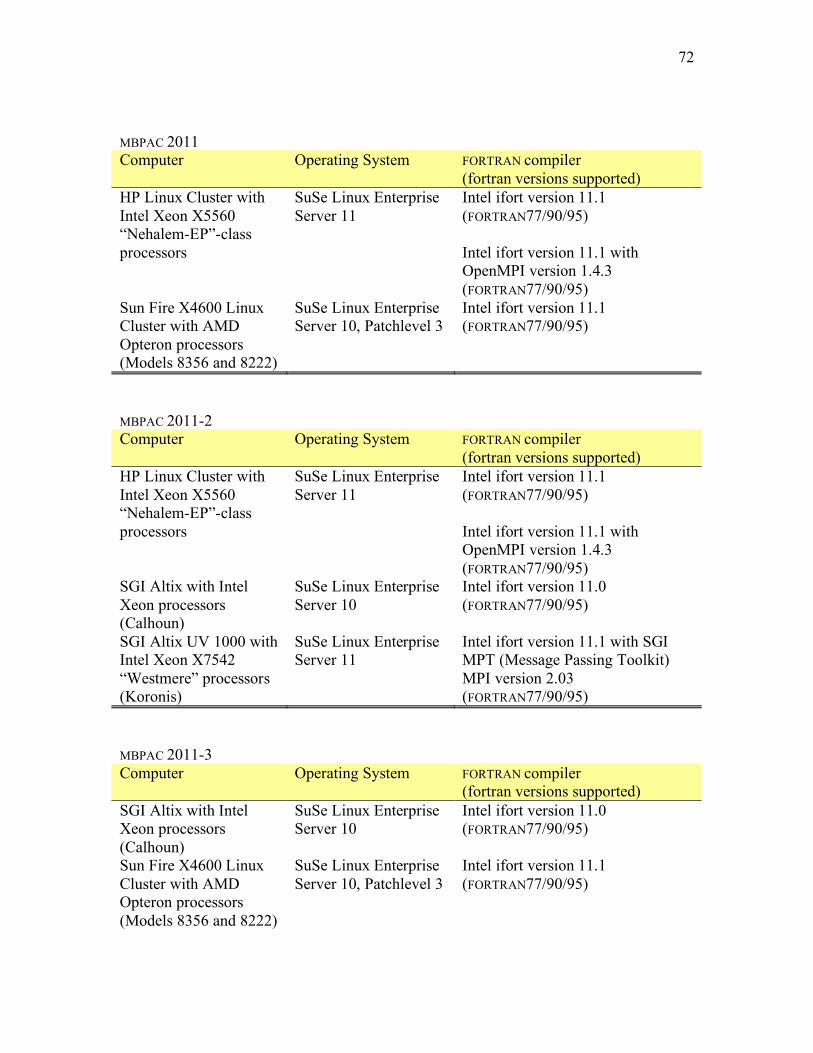
72

MBPAC 2011 Computer Operating System FORTRAN compiler

(fortran versions supported) HP Linux Cluster with Intel Xeon X5560 “Nehalem-EP”-class processors

SuSe Linux Enterprise Server 11

Intel ifort version 11.1 (FORTRAN77/90/95) Intel ifort version 11.1 with OpenMPI version 1.4.3 (FORTRAN77/90/95)

Sun Fire X4600 Linux Cluster with AMD Opteron processors (Models 8356 and 8222)

SuSe Linux Enterprise Server 10, Patchlevel 3

Intel ifort version 11.1 (FORTRAN77/90/95)

MBPAC 2011-2 Computer Operating System FORTRAN compiler

(fortran versions supported) HP Linux Cluster with Intel Xeon X5560 “Nehalem-EP”-class processors

SuSe Linux Enterprise Server 11

Intel ifort version 11.1 (FORTRAN77/90/95) Intel ifort version 11.1 with OpenMPI version 1.4.3 (FORTRAN77/90/95)

SGI Altix with Intel Xeon processors (Calhoun)

SuSe Linux Enterprise Server 10

Intel ifort version 11.0 (FORTRAN77/90/95)

SGI Altix UV 1000 with Intel Xeon X7542 “Westmere” processors (Koronis)

SuSe Linux Enterprise Server 11

Intel ifort version 11.1 with SGI MPT (Message Passing Toolkit) MPI version 2.03 (FORTRAN77/90/95)

MBPAC 2011-3 Computer Operating System FORTRAN compiler

(fortran versions supported) SGI Altix with Intel Xeon processors (Calhoun)

SuSe Linux Enterprise Server 10

Intel ifort version 11.0 (FORTRAN77/90/95)

Sun Fire X4600 Linux Cluster with AMD Opteron processors (Models 8356 and 8222)

SuSe Linux Enterprise Server 10, Patchlevel 3

Intel ifort version 11.1 (FORTRAN77/90/95)

73

HP Linux Cluster with Intel Xeon X5560 “Nehalem-EP”-class processors

SuSe Linux Enterprise Server 11

Intel ifort version 11.1 (FORTRAN77/90/95)

MBPAC 2011-3A Computer Operating System FORTRAN compiler

(fortran versions supported) HP Linux Cluster with Intel Xeon X5560 “Nehalem-EP”-class processors

SuSe Linux Enterprise Server 11

Intel ifort version 11.1 (FORTRAN77/90/95)

MBPAC 2011-4 Computer Operating System FORTRAN compiler

(fortran versions supported and number of processors used)

SGI Altix with Intel Xeon processors (Calhoun)

SuSe Linux Enterprise Server 10

Intel ifort version 11.0 (FORTRAN77/90/95) on 1 processor Intel ifort version 11.0 with OpenMPI version 1.2.8 (FORTRAN77/90/95) on 8 processors

HP Linux Cluster with Intel Xeon X5560 “Nehalem-EP”-class processors

SuSe Linux Enterprise Server 11

Intel ifort version 11.1 (FORTRAN77/90/95) with Platform MPI version 8.0 on 8 processors

MBPAC 2011-5 Computer Operating System FORTRAN compiler

(fortran versions supported and number of processors used)

SGI Altix with Intel Xeon processors (Calhoun)

SuSe Linux Enterprise Server 10

Intel ifort version 10.0 (FORTRAN77/90/95) on 1 processor

74

SGI Altix UV 1000 with Intel Xeon X7542 “Westmere” processors (Koronis)

SuSe Linux Enterprise Server 11

Intel ifort version 11.1 (FORTRAN77/90/95) on 1 processor Intel ifort version 11.1 (FORTRAN77/90/95) with SGI Message Passing Toolkit on 6 processors

MBPAC 2012 Computer Operating System FORTRAN compiler

(fortran versions supported and number of processors used)

HP Linux cluster with Intel Xeon processors (Itasca)

SuSe Linux Enterprise Server 11

Intel ifort version 11.1 (FORTRAN77/90/95) with Platform MPI on 8 processors

SGI Altix UV 1000 with Intel Xeon X7542 “Westmere” processors (Koronis)

SuSe Linux Enterprise Server 11

Intel ifort version 11.1 (FORTRAN77/90/95) on 1 processor

MBPAC 2012-2 Computer Operating System FORTRAN compiler

(fortran versions supported and number of processors used)

SGI Altix UV 1000 with Intel Xeon X7542 “Westmere” processors (Koronis)

SuSe Linux Enterprise Server 11

Intel ifort version 12.1 (FORTRAN77/90/95) on 1 processor Intel ifort version 12.1 (FORTRAN77/90/95) with SGI Message Passing Toolkit on 12 processors

75

MBPAC 2012-3 Computer Operating System FORTRAN compiler

(fortran versions supported and number of processors used)

SGI Altix UV 1000 with Intel Xeon X7542 “Westmere” processors (Koronis)

SuSe Linux Enterprise Server 11

Intel ifort version 12.1 (FORTRAN77/90/95) on 1 processor Intel ifort version 12.1 (FORTRAN77/90/95) with SGI Message Passing Toolkit on 12 processors

MBPAC 2012-4 Computer Operating System FORTRAN compiler

(fortran versions supported and number of processors used)

SGI Altix with Intel Xeon processors (Calhoun)

CentOS 6.2 Intel ifort version 12.1 (FORTRAN77/90/95) on 1 processor Intel ifort version 12.1 (FORTRAN77/90/95) with OpenMPI on 12 processors

MBPAC 2012-4A Computer Operating System FORTRAN compiler

(fortran versions supported and number of processors used)

SGI Altix with Intel Xeon processors (Calhoun)

CentOS 6.2 Intel ifort version 12.1 (FORTRAN77/90/95) with OpenMPI on 12 processors

SGI Altix UV 1000 with Intel Xeon X7542 “Westmere” processors (Koronis)

SuSe Linux Enterprise Server 11

Intel ifort version 12.1 (FORTRAN77/90/95) with SGI Message Passing Toolkit on 12 processors

76

Chapter Eleven

Cited References

(1) Dahlke, E. E.; Truhlar, D. G. J. Phys. Chem. B 2006, 109, 15677.

(2) Frisch, M. J.; Trucks, G. W.; Schlegel, H. B.; Scuseria, G. E.; Robb, M. A.; Cheeseman, J. R.; Scalmani, G.; Barone, V.; Mennucci, B.; Petersson, G. A.; Nakatsuji, H.; Caricato, M.; Li, X.; Hratchian, H. P.; Izmaylov, A. F.; Bloino, J.; Zheng, G.; Sonnenberg, J. L.; Hada, M.; Ehara, M.; Toyota, K.; Fukuda, R.; Hasegawa, J.; Ishida, M.; Nakajima, T.; Honda, Y.; Kitao, O.; Nakai, H.; Vreven, T.; Montgomery, Jr., J. A.; Peralta, J. E.; Ogliaro, F.; Bearpark, M.; Heyd, J. J.; Brothers, E.; Kudin, K. N.; Staroverov, V. N.; Kobayashi, R.; Normand, J.; Raghavachari, K.; Rendell, A.; Burant, J. C.; Iyengar, S. S.; Tomasi, J.; Cossi, M.; Rega, N.; Millam, N. J.; Klene, M.; Knox, J. E.; Cross, J. B.; Bakken, V.; Adamo, C.; Jaramillo, J.; Gomperts, R.; Stratmann, R. E.; Yazyev, O.; Austin, A. J.; Cammi, R.; Pomelli, C.; Ochterski, J. W.; Martin, R. L.; Morokuma, K.; Zakrzewski, V. G.; Voth, G. A.; Salvador, P.; Dannenberg, J. J.; Dapprich, S.; Daniels, A. D.; Farkas, Ö.; Foresman, J. B.; Ortiz, J. V.; Cioslowski, J.; Fox, D. J. Gaussian 09–versions a01 and a02; Gaussian Inc.: Wallingford, CT, 2009.

(3) Werner, H.-J.; Knowles, P. J.; Knizia, G.; Manby, F. R.; Schütz, M.; Celani, P.; Korona, T,; Lindh, R.; Mitrushenkov, A.; Rauhut, G.; Shamasundar, K. R.; Adler, T. B.; Amos, R. D.; Bernhardsson, A.; Berning, A.; Cooper, D. L.; Deegan, M. J. O.; Dobbyn, A. J.; Eckert, F.; Goll, E.; Hampel, C.; Hesselmann, A.; Hetzer, G.; Hrenar, T.; Jansen, G.; Köppl, C.; Liu, Y.; Lloyd, A. W.; Mata, R. A.; May, A. J.; McNicholas, S. J.; Meyer, W.; Mura, M. E.; Nicklass, A.; O'Neill, D. P.; Palmieri, P.; Pflüger, K.; Pitzer, R.; Reiher, M.; Shiozaki, T.; Stoll, H.; Stone, A. J.; Tarroni, R.; Thorsteinsson, T.; Wang, M.; Wolf, A. MOLPRO, version 2010.1, a package of ab initio programs.

(4) Elrod, M. J.; Saykally, R. J. Chem. Rev. 1994, 94, 1975.

(5) Dahlke, E. E.; Truhlar, D. G. J. Chem. Theory. Comp. 2007, 3, 46.

(6) Mulliken, R. S. J. Chem. Phys. 1955, 23, 1833.

(7) Breneman, C. M.; Wiberg, K. B. J. Comp. Chem. 1990, 11, 361.

(8) Xantheas, S. S. J. Chem. Phys. 1994, 100, 7523.

(9) Löwdin, P. O. J. Chem. Phys. 1950, 18, 3654.

(10) Baker, J. Theor. Chim. Acta 1985, 68, 221.

(11) Thompson, J. D.; Xidos, J. D.; Sonbuchner, T. M.; Cramer, C. J.; Truhlar, D. G. PhysChemComm 2002, 5, 1170.

77

(12) Storer, J. W.; Giesen, D. J.; Cramer. C. J.; Truhlar, D. G. J. Comput.-Aided Mol. Design 1995, 9, 872.

(13) Singh, U. C.; Kollman, P. A. J. Comp. Chem. 1984, 5, 129.

(14) Besler, B. H.; Merz Jr., K. M.; Kollman, P. A. J. Comp. Chem. 1990, 11, 431.

(15) Amin, E. A.; Truhlar, D. G. J. Chem. Theory. Comput. 2008, 4, 75.

(16) Wang, B.; Truhlar, D. G. J. Chem. Theory Comput. 2010, 6, 3330.

(17) Dahlke, E. E.; Leverentz, H. R.; Truhlar, D. G. J. Chem. Theory Comput. 2008, 4, 33.

(18) Dolg, M.; Wedig, U.; Stoll, H.; Preuss, H. J. Chem. Phys. 1987, 86, 866.

(19) Igel-Mann, G. Ph.D. Thesis, University of Stuttgart, Stuttgart, 1987.

78

Chapter Twelve

Bibliography

(1) Dahlke, E. E.; Truhlar, D. G. “Electrostatically Embedded Many-Body Expansion for Large Systems, with Applications to Water Clusters” J. Chem. Theory Comput. 2007, 3, 46–53.

(2) Dahlke, E. E.; Truhlar, D. G. “Electrostatically Embedded Many-Body Correlation Energy, with Applications to the Calculation of Accurate Second-Order Møller-Plesset Theory Energies for Large Water Clusters” J. Chem. Theory Comput. 2007, 3, 1342–1348.

(3) Dahlke, E. E.; Truhlar, D. G. “Electrostatically Embedded Many-Body Expansion for Simulations” J. Chem. Theory Comput. 2008, 4, 1–6.

(4) Dahlke, E. E.; Leverentz, H. R., Truhlar, D. G. “Evaluation of the Electrostatically Embedded Many-Body Expansion and the Electrostatically Embedded Many-Body Expansion of the Correlation Energy by Application to Low-Lying Water Hexamers” J. Chem. Theory Comput. 2008, 4, 33–41.

(5) Sorkin, A.; Dahlke, E. E.; Truhlar, D. G. “Application of the electrostatically embedded many-body expansion to microsolvation of ammonia in water clusters” J. Chem. Theory Comput. 2008, 4, 683–688.

(6) Leverentz, H. R.; Truhlar, D. G. “Electrostatically Embedded Many-Body Approximation for Systems of Water, Ammonia, and Sulfuric Acid and the Dependence of Its Performance on Embedding Charges” J. Chem. Theory Comput. 2009, 5, 1573–1584.

(7) Hua, D.; Leverentz, H. R.; Amin, E. A.; Truhlar, D. G. “Assessment and Validation of the Electrostatically Embedded Many-Body Expansion for Metal-Ligand Bonding” J. Chem. Theory Comput. 2011, 7, 251–255.

(8) Tempkin, J. O. B.; Leverentz, H. R.; Wang, B.; Truhlar, D. G. “The Screened Electrostatically Embedded Many-Body Method” J. Phys. Chem. Lett. 2011, 2, 2141–2144.

(9) Kurbanov, E. K.; Leverentz, H. R.; Truhlar, D. G.; Amin, E. A. “Electrostatically Embedded Many-Body Expansion for Neutral and Charged Metalloenzyme Model Systems” J. Chem. Theory Comput. 2012-3, 8, 1–5.

79

Chapter Thirteen

Revision History

13.A. VERSION 1.0

First distributed version

13.B. Version 2007

1. The restart option has been added.

2. The code has been parallelized using MPI.

3. The output has been modified to print the V1, V2, and V3 contributions to the

energy.

13.C. Version 2007-2

1. Gradient calculations have been added.

2. Hessian/frequency calculations have been added.

3. Geometry optimizations with the Gaussian 03 external optimizer have been

implemented.

13.D. Version 2009 (May 28, 2009)

1. In the previous version, the gradient calculations were not correct because the

gradients at the background point charges were left out. Now this has been

corrected in the current version. The new implementation uses the ONIOM

method instead of the previous Gaussian keyword charge. Two new

subroutines getbqap and getbqhp have been added, and modifications have

been made to subroutines: eg09, ehooks, g09oute, g09outg, g09outh,

ghooks, hhooks, main, og09, wg09g, and wg09h as well as scripts

80

g09shuttle and Gau_External_2. The common.inc file was also

revised.

2. For the convenience of users and developers, three scripts have been added:

checktestrun for comparing test run results with those distributed with the

package, updatetestrun for preparing a new testrun directory

(newtestrun), and updatetesto for preparing a new testo directory

(newtesto) that containing the latest test run results.

3. Three test runs (testrun11, testrun12, and testrun13) have been

added, which perform EE-3B energy, gradient, and Hessian calculations on

the system used in testrun8; testrun8 carries out an EE-PA gradient

calculation. Since EE-3B calculations for 3-fragment systems are exact, those

newly added test runs can compared directly with full-QM calculations on the

same system, and can be used to check if the program implementation is

correct (it will not reveal all bugs, but it can be a good test to reveal many

bugs).

4. The testall.pl script is revised, and a testall.pbs script is provided for

submitting the test runs to the queue.

5. Many of the additions to MBPAC2009 were implemented using FORTRAN90.

As a result the G77 compiler and other FORTRAN77 compilers are no longer

supported.

13.E. Version 2009-2 (June 25, 2009)

1. Two new keywords have been added: CORE and KEYWORDS. CORE allows the

user to use effective core potentials, and KEYWORDS allows the user to specify

81

Gaussian 03 keywords for use in the calculation. Changes have been made to

the following files: main.f, eehed.f, ehooks.f, ghooks.f, hhooks.f,

ohooks.f, read.f, and worker.f.

2. Two new test runs (test runs 14 and 15) have been included to illustrate the

new keywords.

3. A new script check_all.pl has been provided to check the results of the test

runs to the output in testo/

13.F. Version 2011 (March 18, 2011)

Authors of the revisions in this version: Hannah Leverentz and Donald G. Truhlar

Complete author list of this version: Erin Dahlke, Hai Lin, Hannah Leverentz, and

Donald G. Truhlar

1. MBPAC now contains calls to Gaussian 09 instead of Gaussian 03. Changes

were made to source files common.inc, eehed.f, ehooks.f, freq.f,

ghooks.f, hhooks.f, main.f, ohooks.f, worker.f, and to scripts

eemb.pl, ex_shuttle, g03-ex-shuttle.pl (now g09-ex-

shuttle.pl), g03shuttle.pl (now g09shuttle.pl), and

Gau_External_2.

2. One new keyword has been added: POPULATION. This keyword allows the user

to specify a method of population analysis that can be used to obtain EE-MB

estimates of partial charges for the entire system. The methods of population

analysis available in this version are Mulliken,6 Merz-Singh-Kollman,13,14 and

CHelpG.7 Changes have been made to the following files: main.f,

eehed.f, ehooks.f, ghooks.f, hhooks.f, ohooks.f, read.f,

82

worker.f, and g09shuttle.pl. Two new subroutines, readqqm and

chkcpop, were added to files ehooks.f and read.f, respectively.

3. EE-MB estimates of the wave function dipole moment are now printed at the

bottom of the output file for every type of calculation, not just for gradient and

hessian calculations. Changes were made to ehooks.f and

g09shuttle.pl.

4. One new test run (test run 16) has been included to illustrate the new keyword.

5. A bug has been fixed that formerly prevented geometry optimizations from

being performed on systems containing more than 10 atoms. Changes were

made to source files ghooks.f and hhooks.f and to the script

ex_shuttle.

13.G. Version 2011-2 (April 13, 2011)

Authors of the revisions in this version: Hannah Leverentz and Donald G. Truhlar

Complete author list of this version: Erin Dahlke, Hai Lin, Hannah Leverentz, and

Donald G. Truhlar

1. The default geometry optimization algorithm in Gaussian 09 is different from

that of Gaussian 03, and, as a result, geometry optimizations in MBPAC 2011

are much slower to converge than they are in earlier versions of MBPAC. In

MBPAC 2011-2, the geometry optimization by the external Gaussian optimizer

is forced to use the same algorithm that was used in Gaussian 03, thus

enabling MBPAC geometry optimizations to converge more efficiently.

Changes were made to source file ohooks.f.

83

2. In previous versions of MBPAC, the EE-MB optimized geometries were

printed in bohr, whereas in this version the coordinates are printed in

Angstroms. Changes were made to source files common.inc and ohooks.f.

3. A bug that had been introduced in version 2011 and which had prevented

MBPAC from being run on systems containing five or more fragments was

corrected: two new variables were added to subroutine eg09 in ehooks.f.

4. Test run 17 was added to allow checking that MBPAC runs successfully on a

system containing five fragments.

5. In version 2011, dipole moments were being printed in atomic units even

though the output file incorrectly stated that the units were debye. Now the

dipole moments are genuinely being printed to the output file in debye.

Changes were made to common.inc, ehooks.f, ghooks.f, and hhooks.f.

13.H. Version 2011-3 (June 21, 2011)

Authors of the revisions in this version: Bo Wang, Hannah Leverentz, and

Donald G. Truhlar

Complete author list of this version: Erin Dahlke, Hai Lin, Hannah Leverentz, Bo

Wang, and Donald G. Truhlar

1. The screened charge model has been added into the serial version of the code

(see keyword SCRCHG in Section 8.C). In this version only energy

calculations are available when the screened charge model is requested;

gradients, Hessians, and geometry optimizations cannot be performed if the

screened charge model is being used. If unscreened embedding charges are

84

being used, then energies, gradients, and Hessians are still available in both

the serial and parallel versions of the program.

2. Test runs 18, 19, and 20 were added as examples of the screened charge model.

3. Major changes were made to subroutine eg09 in ehooks.f and

g09shuttle.pl.

4. Three new subroutines were added: subroutines atomic and chgcorr in

ehooks.f and subroutine gbgqs in frag.f

5. In ehooks.f, added nosym keyword to the setup of normal calculations so

that the full-system calculation of the energy of a trimer will be consistent

with the individual monomer and dimer calculations within the trimer.

6. Increased MAXAPF (the maximum number of atoms allowed per fragment) from

10 to 20 in common.inc.

13.I. Version 2011-3A (July 7, 2011)

Authors of the revisions in this version: Hannah Leverentz

Complete author list of this version: Erin Dahlke, Hai Lin, Hannah Leverentz, Bo

Wang, and Donald G. Truhlar

1. Increased parameter MAXAT (the maximum total number of atoms) in

common.inc from 100 to 200 atoms.

2. Changed dimensions of bgq array in subroutine wsum in file eehed.f from

(maxat,6) to (maxat,5).

85

13.J. Version 2011-4 (July 13, 2011)

Authors of the revisions in this version: Jeremy Tempkin, Hannah Leverentz, and

Donald G. Truhlar

Complete author list of this version: Erin Dahlke, Hai Lin, Hannah Leverentz, Bo

Wang, Jeremy Tempkin, and Donald G. Truhlar

1. The screened charge model has been added into the parallel version of the code

(see keyword SCRCHG in Section 8.C). In this version only energy

calculations are available when the screened charge model is requested;

gradients, Hessians, and geometry optimizations cannot be performed if the

screened charge model is being used. If unscreened embedding charges are

being used, then energies, gradients, Hessians, and geometry optimizations are

still available in both the serial and parallel versions of the program.

2. Changes were made to subroutines eg09 and chgcorr in ehooks.f in both the

serial and parallel versions of the code, and changes were also made to

g09shuttle.pl. The main purpose of these changes is to allow the

calculations with screened charges to be carried out in parallel.

13.K. Version 2011-5 (November 22, 2011)

Authors of the revisions in this version: Bo Wang, Hannah Leverentz, and

Donald G. Truhlar

Complete author list of this version: Hannah Leverentz, Erin Dahlke, Hai Lin, Bo

Wang, Jeremy Tempkin, and Donald G. Truhlar

1. An option to use pseudopotentials on background charges has been added into

the serial and parallel versions of the code.

86

2. A bug is fixed to allow using SCRCHG and CORE options together.

3. The 1-body approximations to dipoles and, when appropriate, the 1-body

approximations to atomic partial charges are now printed to the output file

(previously only the 2- and 3-body approximations to these properties were

being printed).

4. Increased parameter MAXE in common.inc from 10 to 15.

5. Added the EEMBCE keyword to enable the EE-MB-CE approximation to be

used. In this version of the program the EEMBCE keyword can only be used

with single-point energy calculations. Using the EEMBCE keyword with a

gradient, hessian, geometry optimization, or population analysis is not

supported; attempting to use one of these unsupported combinations of

keywords will cause the program to print an error message and stop.

13.L. Version 2012 (February 13, 2012)

Authors of the revisions in this version: Hannah Leverentz and Donald G. Truhlar

(the authors are grateful to Shuxia Zhang and Bo Wang for advice on the

creation of this version)

Complete author list of this version: Hannah Leverentz, Erin Dahlke, Hai Lin, Bo

Wang, Jeremy Tempkin, and Donald G. Truhlar

1. Rather than printing the essential information of the fragment calculations of a

certain type (i.e., monomer, dimer, or trimer) to a single file called 1.eemb,

2.eemb, or 3.eemb, the information pertaining to each fragment is sent to an

individual file with a name having the form x_1.eemb, x_2.eemb, or

x_3.eemb, where x labels the individual monomer, dimer, or trimer. This

87

change makes the parallel version of the code more efficient and also prevents

problems that were arising when more than one processor needed to write

large amounts of information to the same file. In order to accommodate this

change, the serial and parallel versions of subroutines fndstrt, fndstrtg,

and fndstrth have been replaced with subroutines fndstrt2s (for the

serial version) and fndstrt2 (for the parallel version).

2. Frequency calculations have been made more stable by using the

opt=(maxcyc=1,nomicro,cartesian,calcfc) keyword and options

rather than the freq keyword in the Gaussian input files set up by MBPAC.

This change prevents problems that were arising when Gaussian was unable

to convert Cartesian coordinates to internal coordinates for certain

configurations of various systems.

13.M. Version 2012-2 (May 16, 2012)

Authors of the revisions in this version: Hannah Leverentz and Donald G. Truhlar

Complete author list of this version: Hannah Leverentz, Erin Dahlke, Hai Lin, Bo

Wang, Jeremy Tempkin, and Donald G. Truhlar

1. The parallel version has been made more efficient: all monomer, dimer, and

trimer calculations (and the full Hartree–Fock calculation if the EE-MB-CE

option has been selected) can now be run simultaneously during single-point

energy calculations, whereas in previous versions the full Hartree–Fock

portion of an EE-MB-CE calculation would have been done first, then all

monomer calculations would be run in parallel, then all dimer calculations in

parallel, and finally all trimer calculations in parallel. In this version, the

88

gradient and hessian calculations are still done using the older, less efficient

algorithm.

2. Changes have been made to the serial version of the code so that the serial

version uses the same data structures as the parallel version.

13.N. Version 2012-3 (May 23, 2012)

Authors of the revisions in this version: Hannah Leverentz and Donald G. Truhlar

Complete author list of this version: Hannah Leverentz, Erin Dahlke, Hai Lin, Bo

Wang, Jeremy Tempkin, and Donald G. Truhlar

1. The parallel version has been made more efficient for gradient and hessian

calculations.

2. Changes have been made to the serial version of the code so that the serial

version uses the same data structures as the parallel version in the gradient and

hessian calculations.

3. In previous versions, EE-MB-CE calculations could be restarted but the full-

system Hartree–Fock calculation would always be rerun; in this version the

EE-MB-CE calculations can be restarted and the Hartree–Fock calculation

will not be rerun if it has already been done.

13.O. Version 2012-4 (July 11, 2012)

Authors of the revisions in this version: Helena Qi, Hannah Leverentz, and

Donald G. Truhlar

Complete author list of this version: Hannah Leverentz, Erin Dahlke, Hai Lin, Bo

Wang, Jeremy Tempkin, Helena Qi, and Donald G. Truhlar

89

1. The option to use MOLPRO instead of GAUSSIAN for energy calculations, both

EE-MB and EE-MB-CE, has been added.

2. The parameter MAXAT in common.inc was increased from 200 to 400.

13.P. Version 2012-4A (September 27, 2012)

Authors of the revisions in this version: Hannah Leverentz and Donald G. Truhlar

(the authors are grateful to Shuxia Zhang for advice on the creation of this

version)

Complete author list of this version: Hannah Leverentz, Erin Dahlke, Hai Lin, Bo

Wang, Jeremy Tempkin, Helena Qi, and Donald G. Truhlar

1. Different tag numbers have been assigned to the variables in “MPI_Send” and

“MPI_Recv” calls in the parallel version of the code in order to prevent

problems when large calculations are performed, and many messages must be

passed between the master and worker processors.

End of manual