DEPARTMENT AMBULANCE DIVERSION DATA BY …etd.library.vanderbilt.edu/available/etd-07242009-135048/... · DEPARTMENT AMBULANCE DIVERSION DATA BY ... Figure 1 The Chest Clinic Bayesian

A COMPARISON OF BAYESIAN NETWORK STRUCTURE

LEARNING ALGORITHMS ON EMERGENCY

DEPARTMENT AMBULANCE

DIVERSION DATA

BY

Jeffrey Thomas Leegon

Thesis

Submitted to the Faculty of the

Graduate School of Vanderbilt University

in partial fulfillment of the requirements

for the degree of

MASTER OF SCIENCE

in

Biomedical Informatics

August, 2009

Nashville, Tennessee

Approved:

Professor Dominik Aronsky

Professor Ian Jones

Professor Qingxia Chen

Professor Cynthia Gadd

ii

ACKNOWLEDGEMENTS

I would like to thank my committee for guidance and the individual help each has given

me through this process. Particularly I would like to think my advisor, Dominik Aronsky, for

mentoring and encouraging me since I started as an intern in the Department of Biomedical

Informatics. I also would like to thank Subramani Mani and Laura Brown for the

recommendations through the study design process. I appreciate the encouragement the other

faculty, staff, and students, particularly Allison and Jake McCoy, Judith Dexheimer, Shane

Stenner, and John Paulett. Without the National Library of Medicine financial support from

training grant 2-T15 007450-07 none of this would have been possible. I also appreciate the

encouragement of the Green Hills Community Group at Grace Community church and their

willingness to read draft chapters of my thesis and keep me encouraged. But most of all I would

like to thank my dad and mom, Jesse and Joan Leegon, who through each year of education

have continued to encourage and push me on when it was needed.

iii

TABLE OF CONTENTS

Page

ACKNOWLEDGEMENTS .................................................................................................................... ii

LIST OF FIGURES .............................................................................................................................. vi

LIST OF TABLES .............................................................................................................................. viii

CHAPTER

I. INTRODUCTION ...................................................................................................................... 1

II. BACKGROUND ........................................................................................................................ 2

Purpose .................................................................................................................................. 2

Bayesian Networks ................................................................................................................. 3

Discretization ......................................................................................................................... 6

Structure Learning Algorithms ............................................................................................... 7

Greedy Search .............................................................................................................. 8

Max-Min Hill Climbing Algorithm ................................................................................. 8

Tabu Search .................................................................................................................. 9

Augmented Naïve Bayesian Network ........................................................................... 9

Semi-supervised Algorithm ........................................................................................ 12

Expert Learning........................................................................................................... 13

Outcome Metrics ................................................................................................................. 13

Area under the Receiver Operator Characteristic Curve ........................................... 13

Negative Log Likelihood ............................................................................................. 15

Akaike Information Criterion ...................................................................................... 15

Emergency Department Ambulance Diversion .................................................................... 16

Overcrowding and Diversion ...................................................................................... 17

Previous work ............................................................................................................. 18

III. METHODS ............................................................................................................................. 20

iv

Setting .................................................................................................................................. 20

Data ...................................................................................................................................... 21

Operational definition of variables ...................................................................................... 21

Procedures ........................................................................................................................... 25

Discretization .............................................................................................................. 25

Network Creation ....................................................................................................... 29

Evaluation ............................................................................................................................. 30

Outcome Measures .............................................................................................................. 30

IV. RESULTS ................................................................................................................................ 31

Data ...................................................................................................................................... 31

Descriptive Statistics .................................................................................................. 31

Discretization .............................................................................................................. 32

Algorithm Comparison ............................................................................................... 34

V. DISCUSSION .......................................................................................................................... 38

The Data Set ......................................................................................................................... 38

Structure Learning Algorithm Comparison .......................................................................... 38

Comparison Structure Algorithms and the Expert-Created Network .................................. 40

Discretization Methods Comparison .................................................................................... 40

Limitations ............................................................................................................................ 41

VI. FUTURE WORK ..................................................................................................................... 42

Bayesian Network Structure Learning Packages .................................................................. 42

Emergency Department Ambulance Diversion .................................................................... 42

VII. CONCLUSION ........................................................................................................................ 43

APPENDIX

A. DISCRETIZATION RESULTS .................................................................................................... 44

B. FREQUENCY NETWORK STRUCTURES .................................................................................. 49

C. EQUAL WIDTH NETWORK STRUCTURES .............................................................................. 57

v

D. NETWORK EVALUATION RESULTS ........................................................................................ 66

REFERENCES ................................................................................................................................... 73

vi

LIST OF FIGURES

Figure 1 The Chest Clinic Bayesian Network without out any evidence provided .......................... 3

Figure 2 The Chest Clinic network provided with evidence. ........................................................... 4

Figure 3 A DAG representation of conditional independence between heat stroke and a car

overheating given it is a hot day. ..................................................................................................... 6

Figure 4 An example data set discretized to three bins using equal frequency discretization. ...... 6

Figure 5 An example data set discretized to three bins using equal width discretization. ............. 7

Figure 6 An example naive Bayesian network. .............................................................................. 10

Figure 7 An example augmented Naive Bayesian network structure. .......................................... 11

Figure 8 An example of the three relations within the Markov blanket of a variable. ................. 11

Figure 9 Example of how a Markov blanket model could be modified during the augmentation

step. ............................................................................................................................................... 12

Figure 10 An example of three types of ROC curves. .................................................................... 14

Figure 11 How the two years of data were divided into training, validation, and test data sets. 26

Figure 12 Discretization Step 1. ..................................................................................................... 27


Figure 14 Discretization Step 3.. .................................................................................................... 27






vii

Figure 20 AUC performance of each learned BN structure on the data set for predicting diversion

one hour ahead. ............................................................................................................................. 36

Figure 21 Equal Frequency Learned - Augmented Markov Blanket .............................................. 50

Figure 22 Equal Frequency Learned - Augmented Naive Bayesian Network ................................ 51

Figure 23 Equal Frequency Learned - MMHC Learned Structure .................................................. 52

Figure 24 Equal Frequency Learned - Taboo Learned Network .................................................... 53

Figure 25 Equal Frequency Learned - Greedy Search .................................................................... 54

Figure 26 Equal Frequency Learned - Semi-Supervised ................................................................. 55

Figure 27 Equal Frequency Learned - Expert Developed ............................................................... 56

Figure 28 Equal Width Learned - Augmented Markov Blanket ..................................................... 59

Figure 29 Equal Width Learned - Augmented Naive Bayesian Network ....................................... 60

Figure 30 Equal Width Learned - MMHC ....................................................................................... 61

Figure 31 Equal Width Learned -Taboo Search.............................................................................. 62

Figure 32 Equal Width Learned - Greedy Search ........................................................................... 63

Figure 33 Equal Width Learned - Semi-Supervised ........................................................................ 64

Figure 34 Equal Width Learned Expert-developed ........................................................................ 65

viii

LIST OF TABLES

Table 1 Each structure learning algorithm, the package of the implementation, and the type of

algorithm. ....................................................................................................................................... 29

Table 2 Statistics for each variable in train/validation and test data sets. .................................... 32

Table 3 The order and number of bins for each variable when equal frequency discretization was

used. ............................................................................................................................................... 33

Table 4 The order and number of bins for each variable when equal width discretization was

used. ............................................................................................................................................... 33

Table 5 The best performing algorithms for each of the selected metrics. .................................. 35

Table 6 The best BN structures, including the expert network for each of the selected metrics. 36

Table 7 AUC and 95% CI for each algorithm on the predicting diversion one hour in advance data

set................................................................................................................................................... 37

Table 8 The number of links and the resulting number of probability tables for each created

network structure .......................................................................................................................... 37

Table 9 The selected equal frequency discretization ranges for each variable. ............................ 45

Table 10 The AUC for each variable/bin size combination for equal frequency discretization

when added a sole child node of VUH_ED_DIVERSION. ................................................................ 46

Table 11 The selected equal width discretization ranges for each variable. ................................. 47

Table 12 The AUC for each variable/bin size combination for equal width discretization when

added a sole child node of VUH_ED_DIVERSION. ......................................................................... 48

1

CHAPTER I

INTRODUCTION

Modeling using Bayesian methods can be a daunting task to pursue with limited training

in either machine learning or Bayesian statistics. Algorithms specifically designed to learn the

Bayesian network structure for a data set can provide access to those without this training.

Many Bayesian network implementations exist, but are generally aimed at computer scientists

and focus on teaching how the underlying algorithm is programmed. Few studies have

examined “off the shelf” implementations of Bayesian network structure learning algorithms

which could allow an individual with minimal Bayesian model training to build Bayesian

networks.

The study has four aims: 1) to compare different Bayesian network structure learning

different algorithms on real world emergency department ambulance diversion data, 2) to

compare the machine-learned Bayesian network structures to an expert-created Bayesian

network, and 3) to compare how well the different Bayesian network structures generalize to

predict emergency department ambulance diversion up to twelve hours in advance.

2

CHAPTER II

BACKGROUND

This chapter provides the purpose of evaluating Bayesian network structure learning

algorithm packages by using a real world data set of predicting emergency department diversion

data. The Bayesian network (BN) section gives a brief overview of BNs and a high-level

explanation of how they work. The discretization section explains the purpose of discretization

and describes the two discretization methods implemented in the study. The BN structure

learning algorithms section describes the motivation to use automated methods for learning

BNs, and gives a brief explanation of each algorithm included in the study. The last section

focuses on the emergency department processes, the need to predict ambulance diversion, and

previous work related to ambulance diversion prediction.

Purpose

Medical personnel who have limited computer science and machine learning education

frequently use "off the shelf" products to develop BN models rather than constructing the

models themselves. These packages range from implementations developed by the academic

community, which are often free or in the public domain, to commercial applications, costing

thousands of dollars. While individual reviews for specific software packages are available, very

few studies have compared the performance of “off the shelf” BN structure learning algorithms.

3

Bayesian Networks

BNs are machine learning methods which use Bayes' theorem to calculate the

probability that an event will occur. BNs are not a "black box" that obscures the reasoning of

how the probability is calculated, unlike artificial neural networks or support vector machines.

The graphical nature of BNs allows a user to see how information flows through the network

and what the relationships the model represents between the variables. BNs provide methods

to decompose the joint probability tables, which contain the probability of every combination of

events, into a compact structure (1). BNs capture the same information as the joint probability

tables by modeling the conditional relationships among the variables.

Figure 1 shows the Chest Clinic BN, a classic example to demonstrate how BNs work (2;

3). The example is a prototypical medical diagnoses system to identify whether a patient has

tuberculosis, lung cancer, or bronchitis. The arrows between the variables of the network show

a hypothesized cause and effect relationship between the variables. For example, smoking can

Figure 1 The Chest Clinic Bayesian Network without out any evidence provided

4

cause lung cancer or bronchitis, but does not cause tuberculosis. Likewise, visiting Asia can

affect the probability of having tuberculosis, but does not have a direct effect on the probability

of having lung cancer or bronchitis. The two nodes at the bottom of the network represent a

diagnostic test and an observable symptom. The presence of one or more of these diseases

influences both the chest x-ray test result and the patient exhibiting dyspnea (shortness of

breath).

When new evidence is incorporated into a BN, the probabilities of the unobserved

variables are updated. Four pieces of new knowledge could be acquired during a clinical visit for

the Chest Clinic BN: a chest x-ray, history of smoking, foreign travel by the patient, or the

presence of dyspnea in the patient. The network in Figure 2 shows the Chest Clinic network

instantiated with the previously mentioned evidence. The probability of the patient having each

disease is updated based on the new knowledge.

Figure 2 The Chest Clinic network provided with evidence whether the patient visited Asia, smokes, had an abnormal chest X-ray, or has shortness of breath.

5

The full joint probability table for the Chest Clinic network would contain every

combination of all eight variables, which equal 256 different probabilities (2). Representing the

joint probability tables as a BN reduces the number of probabilities to 36 conditional

probabilities. Most real world BNs contain more variables with different numbers of possible

states.

BNs use the concept of conditional independence to simplify "...both the structure of

the model and the amount of computations needed to perform inference and learning ...” (4).

Two variables are said to be conditionally independent when, given a variable, the two other

variables do not affect each other. In probability notation,

.Variables a and b are said to be conditionally independent of each other given c. For

example, the probability of having a heat stroke and a car overheating are conditionally

independent given the day is hot. Having a heat stroke does not affect whether a car overheats

or not, and vice versa. If the day is hot, then the probabilities increase for both heat stroke and

car overheating. Figure 3 shows the graphical representation of this concept. A more detailed

explanation of BNs and conditional independence can be found in (1; 4; 5). Pourret, Naïm, and

Marcot provide a set of examples of how BNs have been applied to real world problems,

including examples in clinical medicine (6).

6

Figure 3 A DAG representation of conditional independence between heat stroke and a car overheating given it is a hot day.

Discretization

Discretization transforms continuous variables into discrete variables while retaining as

much information as possible (7). Two basic methods of discretization are a) equal frequency

and b) equal width.

a) Equal frequency discretization seeks to put an equal number of data points in each

bin (7; 8). Figure 4 shows a data set discretized to three bins using equal frequency

discretization. The algorithm sums up the number of data points in the data set and evenly

distributes them among the bins. Notice the ranges of numbers in each bin are not the same,

but each bin has the same number of data points. The equal frequency discretization in this

instance is not affected by the lack of numbers between two and seven.

1 21 7 7 7 8 8 9

Figure 4 An example data set discretized to three bins using equal frequency discretization. The black bars separate the three bins.

7

b) Equal width discretization determines the bin ranges based on the range of values in

the data set (7; 8). Figure 5 shows the same example data set as used with the frequency

discretization example, but discretized with three bins using equal width discretization. The

algorithm first calculates the width of each bin. For this example the width size equals

(91+1)/3=3. The first bin contains all values less than three. The second bin would contain all

values greater than three, but less than or equal to nine. In this particular data set, no values

exist within the second bin's range. The final third bin contains all values greater than six, which

2/3 of the example data lies within the third bin's range. Over all, the final discretization for the

example data set has two bins containing data.

1 20 7 7 7 8 8 9

Figure 5 An example data set discretized to three bins using equal width discretization. The example only contains one separation, represented by the black bar, because the middle bin did not hold any data points from the example data set

Structure Learning Algorithms

The overall structure of a BN is a directed acyclic graph (DAG). The term DAG comes

from graph theory and consists of vertices and edges. A DAG is a special form of a graph where

all edges are directed and no cycles exist within the graph. Each of the vertices within the DAG is

assigned a specific variable from the data set. The edges represent the relationships between

the variables.

Searching over all possible DAGs, also called the search space for BN structure learning,

for a set of variables to find the best structure is infeasible for all but the most trivial of

8

problems. A DAG with 18 unlabeled has approximately 1.6 * 1043 (rounded to two significant

figures) different possible configurations (9). This number does not account for assigning specific

variables to each node. Finding the structure or the relationships between the variables, for a

BN is an NP-Hard problem (4). A heuristic, or rule of thumb, is the common method to reduce

the overall search space of an NP-hard problem (1; 4). The following sections provide

descriptions of each structure learning algorithm included in the study and an overview of the

heuristic used to search for BN structures.

Greedy Search

Greedy search uses a “greedy” heuristic to find a solution within a search space. The

greedy heuristic selects the move that gives the search the most immediate gain without regard

to the consequences later in the search process (10). Applying greedy search to BN structure

learning, the greedy search starts with a fully disconnected BN. The greedy search then modifies

the current BN by adding, removing, or reversing links while maintaining the DAG requirement

of a BN (5). A comparison metric is supplied to the greedy search method to compare how well

one structure performs against another one. The search continues until a specified number of

moves occur without improving the metric.

Max-Min Hill Climbing Algorithm

The Max-Min Hill-Climbing (MMHC) algorithm is a hybrid method for learning Bayesian

network structures combining constraint-based and search-and-score techniques (11). First,

MMHC uses Max-Min Parents and Children (MMPC) to identify the parents and children of each

variable in the data set. The Max-Min heuristic in MMPC seeks to maximize the minimum

association between a variable and the target given the candidate parents and children. The

9

parents and children information is used to constrain the greedy search (an edge can only be

added if the parent-child link is identified by MMPC). The greedy search returns a DAG that

maximizes the score of a selected evaluation metric.

Tabu Search

Tabu search is a heuristic optimization method which uses a short term memory to

ensure the search explores new areas to prevent being stuck in a local optimum (12; 13). The

exact implementation used in this study is a proprietary version created by BayesiaLab software

creators, a commercial BN system. The tabu search starts with a BN structure without any links.

The operations are the same as the greedy search described above, adding, removing, or

reversing links to find the best next move. The tabu search differs from the greedy search by

adding a short-term memory of the links added between moves. When a change to a link

between two nodes is made, the link is stored in the short-term memory. Tabu search does not

modify any links in the short term memory for a predetermined number of moves (13). The

algorithm stops the search when a better network structure is not found for a set number of

moves.

Augmented Naïve Bayesian Network

Naïve Bayesian networks (NB) make the assumption that all variables in the BNs are

conditionally independent of each other, given the target variable (4; 5). Figure 6 shows the

graphical representation of this relationship. All variables are children of the target variable.

The NB structure creates a computationally efficient model requiring only the conditional

probabilities for each child node given the target variable and the prior probabilities of the

10

target node. While this assumption does not often hold for real life data sets, the NB has shown

strong results as a predictor (5).

Figure 6 An example naive Bayesian network.

The augmented naïve Bayesian algorithm begins with a NB structure as shown in Figure

6, but relaxes the conditional independence assumption between the child variables. After

creating the standard NB structure, the creators of BayesiaLab use a proprietary greedy search

algorithm to find connections between the child nodes. Once the algorithm finishes the greedy

search for relationships between the child variables the network could look as shown in Figure

7. The blue edges are the original edges from the initial NB structure. The red edges are

examples of the potential edges that could be added during the greedy search (14).

11

Figure 7 An example augmented Naive Bayesian network structure. The blue lines represent the links added in the naive Bayesian network phase and the red lines represent potential links added in the unsupervised search stage.

Augmented Markov Blanket

Figure 8 An example of the three relations within the Markov blanket of a variable: parent nodes(blue), child nodes (green), and parents of the children nodes (red).

The Markov blanket for a variable consists of all variables that make it conditionally

independent of all other variables (1). Figure 8 shows the three types of variable relationships

included in the Markov blanket: parents (blue), children (green), and children’s parents (red).

12

Similar to the augmented naïve Bayesian algorithm described above, the augmented Markov

blanket algorithm relaxes the condition that the connections only be made through the target

variable, but allows connections between the parents, children, and children’s parents of the

target. First, the augmented Bayesian network identifies the Markov blanket for the target

variables. Next, Bayesia's proprietary unsupervised greedy search identifies beneficial

relationships between the other variables within the Markov blanket. Figure 9 shows the

original Markov blanket edges in gray. The red and blue edges are examples of edges which

could identified during the greedy search for relationships between the other variables (14).

Figure 9 Example of how a Markov blanket model could be modified during the augmentation step. The solid lines indicate the original links in the Markov blanket. The dashed lines are potential relations learned during the unsupervised step

Semi-supervised Algorithm

The semi-supervised algorithm is an unpublished proprietary algorithm included in

BayesiaLab. The semi-supervised algorithm applies BayesiaLab's Markov Blanket algorithm

recursively (14).

13

Expert Learning

A common method used to develop BN structures is to employ the help of an expert in

the field or use the current literature on the topic to determine the relationships between the

variables (5). Some disadvantages of using only experts and literature are that only currently

known relationships between the variables can be learned, the expert could bias the network,

and it is a time consuming process.

Outcome Metrics

Selection of an outcome metric is an important part of the model building

process. Each metric brings its own interpretation of what model is best, such as discriminatory

ability or the amount of model complexity. Described below are three outcome metrics

included in the study.

Area under the Receiver Operator Characteristic Curve

Receiver operator characteristic (ROC) curves are used as a statistical method to

evaluate the discriminatory ability of a binary classifier. ROC curves have been used in machine

learning, medicine (15), and biomedical informatics (16) as a method to evaluate classifiers. ROC

curves plot the true positive rate of a classifier against the false positive rate to evaluate the

classifier at different thresholds (15). Metz explains, "...ROC curves provide the most

comprehensive description, because they indicate of all of the combinations of sensitivity and

specificity that a diagnostic test is able to provide as the test's 'decision criterion' is varied (17)."

14

Figure 10 An example of three types of ROC curves. The diagonal green line show an ROC curve equivalent to random guessing. The red ROC curve has a large AUC, but the blue curve performs for situation where false positives are high.

Figure 10 shows three ROC curves. The closer to the upper left hand corner of the graph

that the curve lies, the better it perform. If the ROC curve is a diagonal line, like the diagonal

green ROC curve in Figure 10, the classifier performs equivalent to random guessing. If the ROC

curve goes below the diagonal line then the classifier is guessing the opposite of the correct

answer, which can be easily corrected (15).

The area under the ROC curve (AUC) compares two classifiers in a more generalized

manner. The AUC is a commonly used index of ROC curve (16). Perfect AUC is equal to 1, having

the curve in the far left corner; .5 is the equivalent of random guessing, or a diagonal ROC curve

(15). Though the AUC of one classifier may be higher than another, the classifier with the higher

AUC may not be the best performing classifier in all situations. Figure 10 displays an example of

this. The red ROC curve has a higher AUC than blue ROC curve. If a high true positive rate (or

sensitivity) is needed, the blue ROC curve is the better choice because it has a higher sensitivity

(15). An example of when the blue ROC curve would be a better choice is an HIV test. Informing

a HIV- patient they are HIV+ is a better choice than informing a HIV+ person they are HIV-. AUC

15

does act as a simple quantifiable summary measure for ROC curve when the cost function is not

known (15) .

Negative Log Likelihood

The likelihood of a model quantifies the difference between a model's hypothesized

distribution and from the true distribution of the data set. The likelihood function for a model

gives the likelihood the data set was created using the model's parameters (18). The likelihood is

used to select the set of parameters which maximizes the likelihood of the model in relation to

the data. This process is known as maximum likelihood estimation. Using the log of the

likelihood function (LL) makes the calculation easier to compute since the product of multiple

probabilities get subsequently smaller making it more susceptible to computational rounding

errors. The logarithm transformation is a monotonically increasing function. The resulting LL is

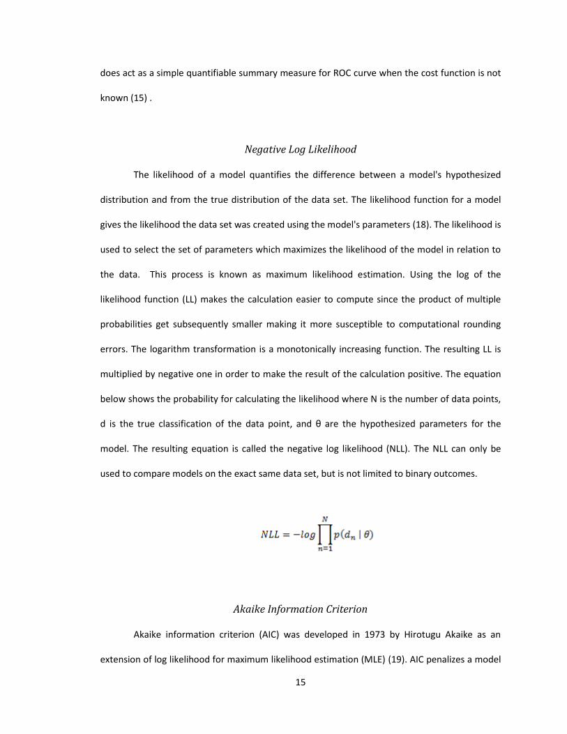
multiplied by negative one in order to make the result of the calculation positive. The equation

below shows the probability for calculating the likelihood where N is the number of data points,

d is the true classification of the data point, and θ are the hypothesized parameters for the

model. The resulting equation is called the negative log likelihood (NLL). The NLL can only be

used to compare models on the exact same data set, but is not limited to binary outcomes.

Akaike Information Criterion

Akaike information criterion (AIC) was developed in 1973 by Hirotugu Akaike as an

extension of log likelihood for maximum likelihood estimation (MLE) (19). AIC penalizes a model

16

for complexity, using the concept of Occam’s razor, which can be summed up as the simplest

explanation is best (20). Below is the equation for AIC where θ is the set of parameters for a

model and k is the number of parameters. The penalty term 2k causes the metric to favor less

complex models to discourage selecting a model which does not generalize well or over fits the

data set used to create the model. A criticism of information criterion which penalizes models

for complexity is that they favor overly simplistic models (20). AIC, like the NLL, is not

generalizable to compare models. AIC must be compared based on the same data set.

Emergency Department Ambulance Diversion

Although time is not a critical factor for most medical care, some patients require

immediate attention. In situations where the patient is having a heart attack or has been in a car

accident, timeliness of care for these patients may significantly affect the potential for loss of

life. To provide timely care most hospitals have an emergency department (ED) open 24 hours a

day to offer care for patients in need of urgent care.

Asplin et al. developed a conceptual model that views the ED as an input-throughput-

output model (21). Following is a description of input, throughput, and output processes at

Vanderbilt University Medical Center’s adult emergency department. A general and detailed

examination of the emergency department as an input-throughput-output model can be found

in (21).

Input (Arrival): Patients arrive at the ED either by ambulance, car, or foot. Patients in

serious condition are taken directly to a treatment area. Patients not in a serious condition upon

arrival are registered and wait to be triaged by a nurse or physician. The nurse or physician uses

17

the criteria of the Emergency Severity Index v3 (ESI) to assign an acuity level (22). The ESI

estimates the amount of ED resources consumed by the patient. Patients not in need of

immediate medical attention are sent to the waiting room and added to a priority queue.

Throughput (Clinical/Treatment): Once in the clinical area patients are placed into one

of nine different types of ED rooms based on the severity of their condition. The physician

examines the patient to determine whether the patient needs laboratory, radiological,

electrocardiogram tests, and/or a consultation.

Output (Discharge): When treatment has been completed the patient is discharged

home, admitted to the hospital, or transferred to another medical care facility.

Overcrowding and Diversion

The Emergency Medical Treatment and Labor Act of 1986 (EMTALA) requires all

hospitals with an ED to treat and stabilize patients without regard to their ability to pay (23).

EMTALA has unfortunately created a significant financial burden for hospitals with EDs because

of the financial loss incurred from patients lacking the ability to pay. The lack of compensation

results in higher prices for those patients with the ability of pay, whether through insurance or

privately. Between 1988 and 1998 the number of EDs in the United States decreased by 28%

(23). In the same period, the number of ED encounters increased by 10%. In addition, the

severity and complexity of patients has increased (24) due to the increasing age of the general

population of the United States (25). Hospital administrators aim to keep hospital occupancy as

close to 100% as possible and in attempt to increase revenue. A full hospital does not allow for

unexpected increases in demand for inpatient beds. This results in ED patients waiting in the ED

for an inpatient bed to become available (25).

18

The ED must divert ambulances when overcrowding reaches a critical point of a risk for

patients currently in the ED or those in transit to the ED due to reduced ability to treat patients.

When this critical point is reached the hospital then informs the ambulance dispatching

authority the ED is going on ambulance diversion because of its inability to safely treat new

incoming critically ill patients. The ambulance authority then sends ambulances to other

hospitals in the area though the overcrowded ED may be the closest. If more than three

hospitals in the area are in a state of ambulance diversion, then the diversion is lifted from all

hospitals. Ambulance diversion leads to an increased amount of time before patients can be

treated, which could increase the severity of their condition. Patients arriving by means other

than ambulance continue to be treated. Once the hospital has reduced the amount of

overcrowding, the hospital alerts the dispatching authority of the ability to accept new

ambulance patients. Identifying the causes of overcrowding is a complex problem with many

factors making diversion difficult to identify in advance. Two reviews of the problem of

emergency department overcrowding can be found in Trzeziak and Rivers (25) and Hoot and

Aronsky (26). Trzeziak and Rivers gives the motivation for predicting ambulance diversion in

advance in order to create a system to provide EDs with a much needed early warning system to

allow ED administrators to: “ ...anticipate and prepare for overcrowding, rather than react to

overcrowding after it has occurred (25)."

Previous work

Solberg et al. (27) gathered 74 experts to determine a generalized set of emergency

department measures for planning, warning, or research. While measurements provide a

standard way to evaluate emergency departments, these metrics are limited because they track

activities over a period of time as explained in the limitations section of the paper.

19

Hoot et al. developed an ED simulation to forecast ED overcrowding 2, 4, 6, and 8 hours

in advance (28). The simulation predicts seven measures related to ED overcrowding: waiting

room count, average waiting time, ED occupancy level, average length of stay, number of

patients waiting to be admitted, the average time a patient waits to be admitted, and the

probability of ambulance diversion. Hoot et al. did a prospective study of the ForcastED

simulation system with respect to the seven measures (29). ForcastED had an AUC of 0.93

predicting two hours in advance to 0.85 for predicting 8 hours in advance. One other study

specifically included ED diversion as a prediction metric. Leegon et al. developed a Gaussian

process for predicting ambulance diversion for up to two hours in advance. The Gaussian

process had an AUC of 0.93 predicting diversion two hours in advance (30). Gaussian processes

are not computationally feasible to implement in real world setting at this time.

20

CHAPTER III

METHODS

The following chapter explains the methodology used for evaluating the BN structure

learning software packages. The setting section provides an overview of technologies

implemented at Vanderbilt University Medical Center (VUMC). The data section describes the

original database and feature selection process that selected the eighteen variables. A summary

from the database specification for each selected variables is in the operational definition of

variable. The procedures section explains the method discretization process, how the BN

structures in each of the software packages were created, and the methods used for evaluation.

Setting

The adult emergency department (ED) at VUMC is a 45 bed Trauma level I,

academic, urban ED. During 2008 the adult ED had more than 55,000 encounters.

VUMC has an information technology infrastructure with computerized order entry (31)

and a longitudinal electronic medical record system (32). In addition to the main

hospital’s information technologies, the ED has an advanced electronic whiteboard

system (33) and computerized triage application (34); both developed internally at

VUMC.

21

Data

A data set was extracted from a locally curated database designed for analyzing ED

overcrowding. The database contained hospital operational information at five minute intervals

with no missing values. All data point for a 2-year period from July 1, 2006 – June 30, 2008 were

included in the study. The data set was subsequently divided into training/validation and test

sets; each contained one year of data. ED ambulance diversion was selected as the reference

standard for identifying overcrowding. The institutional guidelines for when the ED should go on

diversion are 100% occupancy and more than 10 people in the waiting room.

The full curated database contained over 100 variables of operational information for

different parts of the hospital, but focused on the ED and those areas of the hospital likely to

affect the ED. The eighteen variables selected were based on a previous study. In summary, the

study used logistic regression models for an initial screening of each variable in the full

database. The variables were selected based on an AUC above a predefined threshold for each

time point of prediction. All variables in the previous study performing above the defined AUC

thresholds for identifying ambulance diversion 1, 2, 3, 4, 6, 8, and 12 hours in advance were

included in the current study. The current ED diversion status was not included as a predictive

variable to keep subjective variables to a minimum. The final data set used contained eighteen

variables and the ED diversion status from the original database.

Operational definition of variables

An internal VUMC specification contained descriptions for each variable in the

complete database. Below are summaries of the specification definition for each of the 18

variables and the target variable selected for the study.

22

1. VUH_ED_DIVERSION - a Boolean variable indicating the current diversion status of

the ED. VUH_ED_DIVERSION is the reference standard variable for the study.

2. NO_OF_BED_REQUESTS_ED – an integer variable of the number of inpatient bed

requests from the ED.

3. ED_NO_OF_WAITING_ROOM_PTS – an integer variable of the current number of

patients in the waiting room.

4. ED_OCCUPANCY - a real variable ratio of number of patients in all of the ED to the

number of available licensed beds. The value is calculated as:

5. ED_PTS_AVG_TIME_TO_ED_BED – a real variable calculating the average time for a

patient to be placed in a ED bed. The equation below shows the method of

calculation for the average time of placement into an ED bed. Where i is equal to

patients who have been triaged and have not been placed in and ED bed.

6. ED_NO_OF_CURRENT_PTS – an integer variable of the number of patients in the ED.

7. ED_NO_OF_NURSES – an integer variable of the number of nurses who worked in

the ED during the 60 minutes prior to the current time.

23

8. NO_OF_BED_REQUESTS_TRANSFER - an integer variable of the number of admission

requests from patients at other hospitals.

9. ED_VOL_HOSP_CAPACITY_ALL_BDS – a real variable calculating the ratio of ED

volume to hospital capacity for all beds.

10. ED_VOL_HOSP_CAPACITY_ICU_BDS – a real value calculating the ratio of ED volume

to available number of ICU Beds.

11. ED_PTS_AVG_TIME_TO_DISCHARGE – a real variable of the average amount of time

for both inpatient and outpatients to be discharged.

12. ED_INPTS_AVG_TIME_TO_DSCHRG - A real variable of the average time patients

wait in the ED to be admitted to the hospital. Variable i in the equation below is

each patient to be admitted with a bed assigned.

24

13. ED_BED_ASSIGN_TIME_AVG - a real variable of the average time for a patient to be

assigned a bed. Variable i is each patient who has a bed request made for them, but

has not been assigned a bed.

14. ED_INPTS_AVG_LOS_TIME - a real variable of the average length of stay for

inpatients.

15. ED_PTS_AVG_LOS_TIME - a real variable of the average length of stay for both

inpatients and outpatients in minutes.

16. NO_OF_BED_REQUESTS_PERIOP – an integer variable of the number of patients to

be admitted to the hospital from the perioperative service.

17. TOTAL_NO_OF_SURGERY_PER_HR – an integer variable of the number of surgeries

scheduled for the current day.

18. HOSP_AVAIL_BED_CAPACITY - an integer variable of the number of beds available in

the hospital.

19. HOSP_DISCHARGE_POTENTIAL – an integer variable equal to the total number of

occupied inpatient hospital beds minus the number of patients waiting to be

discharged from the hospital.

25

Procedures

The BN structure learning algorithms were evaluated in two steps. The first step

discretized the data as required for each software package; next, the discretized data were input

into each of the BN structure learning algorithms.

Discretization

All implementations of the BN structure learning algorithms included in the study

required the data to be discrete. Discretization was completed prior to BN structure learning to

ensure the individual packages discretization methods were not the actual method being

evaluated. Two unsupervised discretization algorithms were used in the study: equal distance

and equal frequency. Equal distance and equal frequency discretization algorithms were

implemented using a modified version of the Weka data mining libraries source code (35). The

modifications were done to allow the Weka’s implementation of the two discretization methods

to be integrated into the testing framework used for evaluation.

A greedy search approach was used to determine the optimal number of bins for each

variable. Each variable was evaluated with 2- 10 bins. Limiting the number of bins reduced the

overall complexity possible for each network. A naïve Bayesian classifier implemented in the

NeticaJ 4.03 API for Java (3) served as the testing model. The bin sizes and variables were

compared using AUC calculated by PropROC 2.3.1 (36). The comparison was done using the

data set for July 1, 2006 – June 30, 2007. Figure 11 shows how the data set was divided. The

first 70% of the data set was used as training data to determine the parameters of the naïve

Bayesian model. The validation data consisted of the remaining 30%. The validation data was

used to evaluate each variable's performance when added to the naïve Bayesian model. The

26

process was done for both discretization algorithms and resulted in the creation of two data sets

for the study.

100%

Test Data

70 %

Training Data

30%Validation

Data

July 1, 2006 – June 30, 2007 July 1, 2007 – June 30, 2008

Figure 11 How the two years of data were divided into training, validation, and test data sets.

The algorithm evaluated each variable/bin combination's AUC result when the

combination was the only child of the target variable (Figure 12 and Figure 13). The best

performing variable/bin combination was added to the set of selected variables (Figure 14). The

remaining bin sizes for the selected variable were discarded. The variable was fixed as child to

the target variable. Only the top two performing bin sizes for each remaining variable were kept

(Figure 15).

The remaining variable/bin combinations were each added as a child of the target node,

one at a time, to the current set of selected variables (Figure 16). The best performing

variable/bin combination was added to the final bin sizes (Figure 17). The unused bin size for the

selected variable was then discarded (Figure 18). The process continued until all variables had a

bin size chosen (Figure 19).

Once the final discretization ranges for each discretization algorithm were selected,

both the training/validation and test data sets were discretized using each discretization

method.

27

Target

ABins: 3

B

Bins: 3

C

Bins: 3

A

Bins: 4

B

Bins: 4

C

Bins: 4

A

Bins: 5

B

Bins: 5

C

Bins: 5

Figure 12 Target is the variable to be predicted. A, B, and C are the variables in the data set. In this example each variable have been discretized to have 3 – 5 bins.

Target

ABins: 3

AUC: .801

BBins: 3

AUC: .856

CBins: 3

AUC: .654

ABins: 4

AUC: .822

BBins: 4

AUC: .874

CBins: 4

AUC: .635

ABins: 5

AUC: .786

BBins: 5

AUC: .904

C

Bins: 5

Figure 13 Each variable/bin combination were made the only child node of the target and evaluated.

Target

ABins: 3

AUC: .801

BBins: 3

AUC: .856

CBins: 3

AUC: .654

ABins: 4

AUC: .822

BBins: 4

AUC: .874

CBins: 4

AUC: .635

ABins: 5

AUC: .786

BBins: 5AUC: .904

CBins: 5

AUC: .674

Figure 14 After all variables have been evaluated the best variable/bin combination was fixed as a child in the naïve Bayesian network.

Target

ABins: 3

CBins: 3

ABins: 4

BBins: 5

C

Bins: 5

Figure 15 The remaining variables for B are removed. Only the top two performing bin sizes for A and C are kept.

28

Target

ABins: 3

AUC: .824

CBins: 3

ABins: 4

BBins: 5

C

Bins: 5

Figure 16 The remaining variable/bin size combinations were added one at a time to the current network and evaluated.

Target

ABins: 3

AUC: .824

CBins: 4AUC: .898

ABins: 4AUC: .912

BBins: 5

CBins: 5

AUC: .902

Figure 17 Once all variable/bin size combinations have been evaluated the best combination was selected and added to the network.

Target

CBins: 4

ABins: 4

BBins: 5

CBins: 5

Figure 18 This process continued through the remaining variables.

Target

CBins: 4

AUC: .923

ABins: 3

BBins: 5

CBins: 5AUC: .931

Figure 19 The algorithm terminated when all variables have had a bin size selected.

29

Network Creation

Table 1 Each structure learning algorithm, the package of the implementation, and the type of algorithm.

Algorithm Software Algorithm Type

Augmented Naïve Bayes Bayesia ® BayesiaLab Supervised

Augmented Markov Blanket Bayesia ® BayesiaLab Supervised

Greedy Search Causal Explorer Unsupervised

Max-Min Hill Climbing Causal Explorer Unsupervised

Semi-supervised Bayesia ® BayesiaLab Semi-supervised

Tabu Search Bayesia ® BayesiaLab Unsupervised

Six BN structure algorithms implemented by two Bayesian network applications,

BayesiaLab and Causal Explorer, were included in the study. Bayesia® BayesiaLab 4.5.1 (37), is a

commercially developed application for data mining and Bayesian network creation, and Causal

Explorer 1.4 (38) is an academically developed toolbox for MatLab containing several BN

structure algorithms. All Causal Explorer algorithms were executed in MatLab version 14 release

2008b (39). All included algorithms guaranteed a DAG would be created. The supervised

algorithms focus on developing the network structure to predict a specific variable. The

unsupervised algorithms develop a general structure based on relationships between all

included variables. In addition to the machine learning methods, a previous, expert-developed

Bayesian network was included for comparison. Table 1 lists the algorithms included in the

study.

Each application developed Bayesian network structure was learned on the whole

train/validation data set for predicting diversion one hour in advance. The default methodology

for creating the Bayesian network structure was used for each algorithm. The MMHC algorithm

was only supplied with a data set sampled every 15 minutes rather than 5 minutes to reduce the

amount of computation time required for generating a DAG.

30

The expert-developed BN was previously created with the same data set for predicting

ambulance diversion one hour in advance as supplied to the machine learning algorithms. All

algorithms used data discretized the same way.

Evaluation

Each resulting Bayesian network structure was recreated in the BN application Norsys

Netica 4.02 (3). Each BN structure was trained and evaluated on data to predict ambulance

diversion at 1, 2, 4, 6, 8, and 12 hours in advance. The network parameters were learned using

the Norsys® NeticaJ 4.03 API for Java from the entire training/validation set using the counting

method. The counting method calculates the BN parameters by counting the number of times

each conditional probability occurs in the data set. The counting method was selected over the

Expectation-Maximization (EM) algorithm because the data set did not contain missing values

and it takes more time to obtain the same result as counting method (40).

Outcome Measures

The AUC and its 95% confidence interval (CI), negative log likelihood (NLL), and Akaike

Information Criterion (AIC) were calculated on the test data set not used during discretization or

model creation. NLL and AIC were selected as additional methods of evaluation because of their

use in model selection.

31

CHAPTER IV

RESULTS

Data

Descriptive Statistics

The study's training/validation set contained 104,975 observations and the emergency

department was on ambulance diversion 23.2% of the time. The test set, which contained leap

year day for 2008, contained 105,265 observations. The ED was on ambulance diversion 22.3%

of the time during the test set. Table 2 statistics for each variable in train/validation and test

data sets. Table 2 gives the descriptive statistics for the train/validation data sets prior to

discretization.

32

Table 2 statistics for each variable in train/validation and test data sets.

Variable NameTraining

Mean

Training

Standard

Deviation

Test

Mean

Test

Standard

Deviation

NO_OF_BED_REQUESTS_ED 10.26 7.05 11.93 7.64

ED_NO_OF_WAITING_ROOM_PTS 4.55 5.50 4.39 5.31

ED_OCCUPANCY 0.80 0.19 0.82 0.22

ED_PTS_AVG_TIME_TO_ED_BED 26.84 37.56 26.51 38.55

ED_NO_OF_CURRENT_PTS 45.97 13.85 45.99 14.73

NO_OF_BED_REQUESTS_PERIOP 4.28 5.12 3.71 4.82

TOTAL_NO_OF_SURGERY_PER_HR 62.77 35.13 61.12 33.90

ED_NO_OF_NURSES 12.96 1.87 12.96 1.87

HOSP_AVAIL_BED_CAPACITY 21.77 38.78 33.09 35.84

NO_OF_BED_REQUESTS_TRANSFER 26.08 12.30 22.98 10.24

ED_VOL_HOSP_CAPACITY_ALL_BDS 0.17 0.13 0.16 0.13

ED_VOL_HOSP_CAPACITY_ICU_BDS 0.38 0.30 0.38 0.32

ED_PTS_AVG_TIME_TO_DISCHARGE 415.67 263.29 423.74 269.01

ED_INPTS_AVG_TIME_TO_DSCHRG 456.95 274.61 461.56 279.12

HOSP_DISCHARGE_POTENTIAL 0.03 0.03 0.04 0.05

ED_BED_ASSIGN_TIME_AVG 443.81 285.61 459.31 280.76

ED_INPTS_AVG_LOS_TIME 552.14 255.47 607.22 289.98

Discretization

Table 3 shows the order each equal frequency discretized variable was selected.

Table 4 shows the same information as the equal frequency ordering, but for each equal width

discretized variable. Appendix A contains the bin ranges for each method and the AUCs for the

first pass of discretization where each variable/bin combination was made the sole child of the

target variable.

33

Table 3 shows the order and number of bins for each variable when equal frequency discretization was used.

Order

AddedVariable Name

Bin

Size

1 ED_NO_OF_NURSES 2

2 ED_NO_OF_WAITING_ROOM_PTS 3

3 ED_INPTS_AVG_LOS_TIME 4

4 HOSP_AVAIL_BED_CAPACITY 4

5 TOTAL_NO_OF_SURGERY_PER_HR 8

6 ED_PTS_AVG_TIME_TO_DISCHARGE 4

7 NO_OF_BED_REQUESTS_PERIOP 3

8 NO_OF_BED_REQUESTS_TRANSFER 2

9 ED_OCCUPANCY 4

10 ED_BED_ASSIGN_TIME_AVG 5

11 ED_INPTS_AVG_TIME_TO_DSCHRG 4

12 ED_VOL_HOSP_CAPACITY_ALL_BDS 2

13 ED_PTS_AVG_LOS_TIME 2

14 NO_OF_BED_REQUESTS_ED 3

15 ED_NO_OF_CURRENT_PTS 10

16 ED_VOL_HOSP_CAPACITY_ICU_BDS 2

17 HOSP_DISCHARGE_POTENTIAL 4

18 ED_PTS_AVG_TIME_TO_ED_BED 10

Table 4 shows the order and number of bins for each variable when equal width discretization was used.

Order

AddedVariable Name

Bin

Size

1 ED_PTS_AVG_TIME_TO_ED_BED 5

2 ED_NO_OF_WAITING_ROOM_PTS 10

3 ED_INPTS_AVG_LOS_TIME 2

4 HOSP_AVAIL_BED_CAPACITY 3

5 TOTAL_NO_OF_SURGERY_PER_HR 3

6 ED_PTS_AVG_TIME_TO_DISCHARGE 2

7 NO_OF_BED_REQUESTS_PERIOP 2

8 NO_OF_BED_REQUESTS_TRANSFER 7

9 ED_OCCUPANCY 3

10 ED_BED_ASSIGN_TIME_AVG 2

11 ED_INPTS_AVG_TIME_TO_DSCHRG 2

12 ED_VOL_HOSP_CAPACITY_ALL_BDS 2

13 ED_PTS_AVG_LOS_TIME 4

14 NO_OF_BED_REQUESTS_ed 2

15 ED_NO_OF_CURRENT_PTS 3

16 ED_VOL_HOSP_CAPACITY_ICU_BDS 3

17 HOSP_DISCHARGE_POTENTIAL 3

18 ED_NO_OF_NURSES 3

34

Algorithm Comparison

Table 5 gives an overview of the best performing machine learned BN structures. Table 6gives the same overview as

Table 5, but includes the expert-developed network for comparison. Figure 20 plots the

AUC for each BN structure data set for predicting diversion one hour advanced, the data set the

structure was developed.

gives the AUC and 95% CI for the data graphed in Figure 20. Table 7 shows the overall

complexity for each network created for each algorithm, using each discretization algorithm. All

algorithms included 18 variables plus the diversion status except for the augmented Markov

Blanket which had 16 nodes and the expert-developed network which had 11 in addition to the

ambulance diversion status. Diagrams of all Bayesian network structures created using the equal

frequency discretized data set can be found in Appendix B and the network structures created

using the equal width data set can be found in Appendix C. The complete tables of results for all

prediction times can be found in Appendix D.

35

Table 5 The best performing algorithms for each of the selected metrics. The letter attached to the end of the algorithm indicates whether it was the network where equal frequency (F) discretization was used or equal width (W) discretization. Where Area Under ROC has multiple networks list, the networks 95% Confidence Intervals overlapped. The table only includes the structure learning algorithms.

Prediction

TimeArea Under ROC

Negative Log

Likliehood

Akaike Information

Criterion

1 Hour MMHC-F MMHC-F Semi-Supervised-W

2 Hours MMHC-F MMHC-F Tabu-W

4 Hours Tabu-W Tabu-W Tabu-W

Augmented Markov

Blanket-W

6 Hours Tabu-W Tabu-W Tabu-W

Augmented Naïve

Bayes-W

8 Hours Augmented Naïve

Bayes-W

Augmented Markov

Blanket-W

Augmented Markov

Blanket-W

Augmented Markov

Blanket-W

12 Hours Augmented Naïve

Bayes-W

Semi-Supervised-F Augmented Markov

Blanket-W

36

Table 6 contains the best BN structures, including the expert network for each of the selected metrics. The letter attached to the end of the algorithm indicates whether the network was learned on the equal frequency (F) discretized data or equal width (W) discretized data. Where Area under the ROC has multiple networks list, the networks 95% Confidence Intervals overlapped. The table only both machine learned structures and the expert developed network

Prediction

TimeArea Under ROC

Negative Log

Likliehood

Akaike Information

Criterion1 Hour MMHC-F MMHC-F Expert Created -W

Expert Created -F MMHC-F

2 Hours Expert Created -F Expert Created-W Expert Created -W

MMHC-F

4 Hours Expert Created -F Tabu-W Expert Created -W

6 Hours Expert Created-F Tabu-W Expert Created -F

8 HoursExpert Created -F

Augmented Markov

Blanket-WExpert Created -F

Augmented Naïve

Bayes-W

Augmented Markov

Blanket-W

12 Hours Augmented Naïve Semi_Supervised-F Expert Created -F

Figure 20 AUC performance of each learned BN structure on the data set for predicting diversion one hour ahead.

37

Table 7 AUC and 95% CI for each algorithm on the predicting diversion one hour in advance data set

.

Algorithms AUC

Aug Markov 0.9198 0.918 0.922

Aug NB 0.9229 0.921 0.925

Semi-Supervised 0.9449 0.943 0.946

Taboo 0.9449 0.944 0.946

MMHC 0.9491 0.948 0.950

Greedy Search 0.9168 0.915 0.919

Expert 0.9473 0.946 0.949

Algorithms AUC

Aug Markov 0.9421 0.941 0.944

Aug NB 0.9352 0.934 0.937

Semi-Supervised 0.9460 0.945 0.947

Taboo 0.9427 0.941 0.944

MMHC 0.9395 0.938 0.941

Greedy Search 0.9334 0.932 0.935

Expert 0.9395 0.938 0.941

Confidence Interval

Confidence Interval

Equal Width Discretized

Equal Frequency Discretized

Table 8 The number of links and the resulting number of probability tables for each created network structure

Algorithms

Number of Links

Between Nodes

Total Number of

Conditional

Probabilities

Number of Links

Between Nodes

Total Number of

Conditional

ProbabilitiesAug Markov 58 8069 53 3083

Aug NB 66 8994 64 4382

Semi-Supervised 68 13730 57 3331

Taboo 63 6853 56 3397

MMHC 53 5244 60 8430

Greedy Search 76 215966 82 32994

Expert 19 365 19 653

Equal Frequency Discretized Networks Equal Width Discretized Networks

38

CHAPTER V

DISCUSSION

Six different BN structure learning algorithms were used to create two DAGs learned

from a data set to predict diversion one hour in advance. Each algorithm created a DAG for both

of the discretization methods used. The AUC, NLL, and AIC were calculated as an output metrics.

In this chapter we discuss the quality of the data set, how the machine learned DAGs performed

in relation to each other, compare the machine learned structures to the expert-developed

network, and evaluate how well the DAGs generalized predicting ambulance diversion to predict

up to twelve hours ahead.

The Data Set

The train/validation and test data set both contained over 100,000 data points, neither

of which contained any missing values. The reference standard of ED diversion was not perfect.

The institutional guidelines state the ED is to go on ambulance diversion when the occupancy is

greater than or equal 100% and there are 10 or more patients in the waiting room. In the

train/validation data set the ED was on diversion 80% of the time when these criteria were met

and 78% of the time for the test set.

Structure Learning Algorithm Comparison

Table 6 lists the best performing algorithms for each of the selected metrics. The letter

attached to the end of the algorithm indicates whether the BN structure was learned from the

equal frequency (F) or equal width (W) discretization data set. When the AUC field in the table

39

has multiple BNs, this indicates their 95% CI overlap. Except for the BN structures learned from

the augmented Markov blanket algorithm, all machine learning algorithms included each of the

18 variables in the structure. Both the structures learned by the augmented Markov blanket

algorithm on the equal width and equal frequency data sets excluded the

ED_VOL_HOSP_CAPACITY_ALL_BDS and ED_VOL_HOSP_CAPACITY_ICU_BDS variables. These

two variables not being included in the network indicates they did not lie within the identified

Markov Blanket. This implies the nodes did not have a direct effect on the target variable. Their

inclusion in the other graphs indicates ED_VOL_HOSP_CAPACITY_ALL_BDS and

ED_VOL_HOSP_CAPACITY_ICU_BDS had some effect on at least one of the other variables

within the network.

Notice in Figure 20 the best performing networks for predicting diversion 1, 2, and 4

hours in advance favored unsupervised algorithms. Since all structures were learned on the data

set for predicting diversion one hour in advance, the unsupervised algorithms seem to identify

the relationships between all variables in the data set. This could indicate the variables which

affect diversion at 1, 2, and 4 hours in advance are closely related.

The reason the targeted algorithms performed better when predicting diversion after 4

hours may be that the relationships between the variables predicting diversion in advance

change. For the two included supervised algorithms, the overall structures would not likely

change. These naïve targeted structures develop a skeleton structure based on the target

variable before looking for relationships between any of the other variables.

For example, the augmented naïve Bayesian structure first creates a naïve Bayesian

network. This initial network structure would be the same regardless of which diversion

prediction data set was used. The only relationships learned that would be dependent on the

40

relationships between the variables at the specified amount of time in advance, but the

underlying structure would be the same.

Comparison Structure Algorithms and the Expert-Created Network

The expert-developed BN was among the best performing networks for both AUC and

AIC up to 8 hours in advance. Eight hour and above the relationships between the variables

could have changed. The expert network used only 11 variables compared to the machine

learned structures which used between 16 and 18 variables. The expert-developed network also

contained fewer links than the BNs learned by the structure learning algorithms and had fewer

conditional probability tables. The lower complexity alone would be a reason why the expert-

developed network performed best using AIC. The expert-developed network incurred a much

smaller penalty for complexity compared to the machine learned structures.

Though the expert-developed model was simpler, MMHC performed just as well on the

data sets to predict diversion one and two hours in advance. If discriminative ability is the

primary concern, MMHC makes an excellent choice because a human is involved in the

preprocessing of the data, as would also be required to human develop a BN. The user is only

required to allow MMHC develop the DAG, but the many links make it difficult to learn relations.

Discretization Methods Comparison

The BN complexity was a result of discretization showing it to be a factor affecting the

performance of the learned BNs. Each BN structure learning algorithm created two structures,

one for each discretization method. When predicting diversion one hour in advance, the simpler

network created by the algorithm consistently performed better or was within the 95% CI for

earlier predicting networks. The equal width discretization tended to result in the less complex

41

networks. Of the machine learned network structures MMHC was the only algorithm which

created a simpler network using the frequency discretized data set. Overall, the results showed

discretization was a factor in BN creation because networks with fewer conditional probabilities

performed better than their more complex counterparts for all, but prediction times less than

diversion eight hours. Equal width discretization led to simpler networks for all, except MMHC.

Limitations

The study was limited by the number of data sets used for evaluation. Before any

general conclusions could further be made, a broader number of data sets would be needed. In

addition to the use of a single data set, a limited number of discretization methods were used

prior to model building. The simpler models performed best between the two, showing

discretization affected the results.

42

CHAPTER V

FUTURE WORK

Further exploration in both the comparison of BN structure learning packages

along with developing a BN for predicting ambulance diversion in advanced are needed.

Bayesian Network Structure Learning Packages

Future work evaluating BN structure learning packages could be expanded in several

ways. The next step in future work is to include a larger number of algorithms for comparison.

The results should be based on more data sets each discretized using a more expansive number

of techniques.

Emergency Department Ambulance Diversion

For ambulance diversion, the network should be learned on each of the time points the

network is expected to predict rather than learning just one network for all times. Another

possibility would be to use a score metric like the BDeu score to learn a network structure

containing all desired prediction times in a single network. Learning on the additional times

could provide valuable information regarding the relationships between these elements.

Manual modification of the machine learned BN structures by experts could result in less

complex models. Bayesian models which specifically integrate the temporal relationships

between the variables with regard to time, such as dynamic Bayesian networks, hidden Markov

models, or Kalman filters should be examined.

43

CHAPTER VI

CONCLUSION

The results showed the BN algorithms ability to learn models with strong

discrimination. Most of the machine learned structures were able to perform as well as the

expert-developed network. The study showed on the curated data set BN structure algorithms

can create models with strong discriminatory power. These “off the shelf” implementations of

BN structure learning algorithms can provide those with entry level machine learning knowledge

the ability to develop BN models.

44

APPENDIX A

DISCRETIZATION RESULTS

45

Table 9 The selected equal frequency discretization ranges for each variable.

Equal Frequency Discretization

Variable Names

Ranges

ED_NO_OF_CURRENT_PTS

−∞ 27.5 34 37.5 41.5 45.5 49.5 53.5 58.5 65.5 ∞

ED_PTS_AVG_TIME_TO_ED_BED

−∞ 0.5 5.5 12.5 22.5 33.5 46.5 60.5 77.5 101.5 ∞

TOTAL_NO_OF_SURGERY_PER_HR

−∞ 9.5 14.5 71.5 79.5 84.5 89.5 94.5 ∞

ED_BED_ASSIGN_TIME_AVG

−∞ 162.5 357.5 524.5 693.5 ∞

HOSP_DISCHARGE_POTENTIAL

−∞ 0.005 0.010 0.045 ∞

ED_OCCUPANCY

−∞ 0.675 0.845 0.955 ∞

ED_INPTS_AVG_TIME_TO_DSCHRG

−∞ 238.5 462.5 658.5 ∞

ED_PTS_AVG_TIME_TO_DISCHARGE

−∞ 202.5 418.5 612.5 ∞

ED_INPTS_AVG_LOS_TIME

−∞ 347.5 539.5 733.5 ∞

HOSP_AVAIL_BED_CAPACITY

−∞ -12.5 14.5 43.5 ∞

NO_OF_BED_REQUESTS_ED

−∞ 6.5 14.5 ∞

NO_OF_BED_REQUESTS_PERIOP

−∞ 0.5 5.5 ∞

ED_NO_OF_WAITING_ROOM_PTS

−∞ 1.5 5.5 ∞

NO_OF_BED_REQUESTS_TRANSFER

−∞ 26.5 ∞

ED_VOL_HOSP_CAPACITY_ALL_BDS

−∞ 0.135 ∞

ED_PTS_AVG_LOS_TIME

−∞ 401.5 ∞

ED_VOL_HOSP_CAPACITY_ICU_BDS

−∞ 0.305 ∞

ED_NO_OF_NURSES −∞ 12.950 ∞

46

Table 10 The AUC for each variable/bin size combination for equal frequency discretization when added a sole child node of VUH_ED_DIVERSION.

AUC's From First Pass of Frequency Discretization

Frequency Bin Sizes

Variable Names

2

3

4

5

6

7

8

9

10


0.745

0.755

0.757

0.758

0.757

0.759

0.759

0.759

0.761


0.721

0.708

0.708

0.709

0.710

0.710

0.711

0.711

0.711


0.676

0.671

0.663

0.675

0.684

0.648

0.686

0.684

0.677


0.549

0.564

0.577

0.573

0.539

0.553

0.560

0.563

0.557


0.538

0.555

0.545

0.522

0.533

0.532

0.543

0.539

0.536

ED_OCCUPANCY

0.723

0.716

0.720

0.714

0.711

0.715

0.716

0.712

0.711


0.567

0.575

0.589

0.586

0.585

0.561

0.568

0.572

0.575


0.569

0.572

0.579

0.579

0.577

0.578

0.563

0.567

0.569


0.521

0.529

0.531

0.516

0.519

0.524

0.512

0.516

0.519


0.571

0.580

0.574

0.572

0.563

0.567

0.561

0.559

0.557


0.615

0.614

0.603

0.607

0.605

0.610

0.610

0.609

0.608


0.761

0.647

0.647

0.645

0.645

0.646

0.646

0.646

0.647


0.738

0.723

0.715

0.717

0.717

0.717

0.717

0.717

0.717


0.553

0.553

0.545

0.552

0.551

0.554

0.546

0.546

0.547


0.621

0.601

0.605

0.603

0.603

0.599

0.602

0.600

0.603

ED_PTS_AVG_LOS_TIME

0.557

0.540

0.540

0.538

0.541

0.546

0.546

0.542

0.545


0.636

0.629

0.632

0.630

0.628

0.628

0.629

0.629

0.628

ED_NO_OF_NURSES 0.802 0.780 0.779 0.776 0.775 0.777 0.777 0.776 0.776

47

Table 11 The selected equal width discretization ranges for each variable.

Equal Width Discretization

Variable Names

Ranges


−∞ 3.40 6.80 10.20 13.60 17.00 20.40 23.80 27.20 30.60 ∞


−∞ 10.57 20.14 29.71 39.29 48.86 58.43 ∞


−∞ 64.60 129.20 193.80 258.40 ∞

ED_PTS_AVG_LOS_TIME

−∞ 371.00 635.00 899.00 ∞


−∞ 0.00 82.00 ∞


−∞ 39.33 76.67 ∞


−∞ 36.33 63.67 ∞


−∞ 1.22 2.45 ∞


−∞ 0.06 0.11 ∞

ED_OCCUPANCY

−∞ 0.50 0.89 ∞

ED_NO_OF_NURSES

−∞ 12.00 14.00 ∞


−∞ 20.50 ∞


−∞ 876.50 ∞


−∞ 780.00 ∞


−∞ 0.64 ∞


−∞ 746.50 ∞


−∞ 17.50 ∞

ED_INPTS_AVG_LOS_TIME −∞ 896.00 ∞

48

Table 12 The AUC for each variable/bin size combination for equal width discretization when added a sole child node of VUH_ED_DIVERSION.

AUC's From First Pass of Width Discretization

Width Bin Sizes

Variable Names

2

3

4

5

6

7

8

9

10


0.769

0.766

0.760

0.765

0.765

0.755

0.757

0.760

0.760


0.674

0.593

0.708

0.882

0.876

0.866

0.806

0.788

0.783


0.639

0.676

0.639

0.648

0.658

0.668

0.626

0.632

0.616


0.662

0.600

0.541

0.562

0.552

0.558

0.560

0.545

0.557


0.553

0.558

0.518

0.525

0.516

0.520

0.520

0.521

0.521

ED_OCCUPANCY

0.732

0.739

0.701

0.707

0.720

0.708

0.708

0.704

0.705


0.661

0.574

0.579

0.567

0.569

0.577

0.572

0.570

0.570


0.651

0.591

0.573

0.562

0.567

0.571

0.568

0.570

0.569


0.527

0.530

0.518

0.519

0.514

0.521

0.513

0.520

0.511


0.500

0.579

0.552

0.555

0.544

0.574

0.565

0.556

0.551


0.633

0.606

0.611

0.597

0.605

0.601

0.599

0.594

0.600


0.847

0.828

0.638

0.654

0.645

0.638

0.636

0.646

0.646


0.825

0.667

0.675

0.697

0.717

0.718

0.725

0.726

0.726


0.544

0.545

0.543

0.542

0.539

0.558

0.545

0.552

0.543


0.627

0.700

0.603

0.599

0.601

0.602

0.606

0.608

0.606

ED_PTS_AVG_LOS_TIME

0.500

0.543

0.571

0.530

0.540

0.554

0.554

0.543

0.555


0.728

0.804

0.759

0.611

0.643

0.641

0.630

0.627

0.636

ED_NO_OF_NURSES

0.802 0.780 0.777 0.776 0.777 0.777 0.776 0.776 0.776

49

APPENDIX B

FREQUENCY NETWORK STRUCTURES

50

Figure 21 Augmented Markov Blanket

51

Figure 22 Augmented Naive Bayesian Network

52

Figure 23 MMHC Learned Structure

53

Figure 24 Taboo Learned Network

54

Figure 25 Greedy Search

55

Figure 26 Semi-Supervised

56

Figure 27 Expert Developed

57

APPENDIX C

EQUAL WIDTH NETWORK STRUCTURES

58

59

Figure 28 Markov Blanket

60

Figure 29Augmented Naive Bayesian Network

61

Figure 30 MMHC

62

Figure 31 Taboo Search

63

Figure 32 Greedy Search

64

Figure 33 Semi-Supervised

65

Figure 34 Expert-developed

66

APPENDIX D

NETWORK EVALUATION RESULTS

67

Predicting 1 hour in Advance

Equal Frequency Discretized Data Set

Algorithms AUC

SE of AUC

NLL

AIC

Aug Markov 0.9198

8.88E-04

35757.05

87652.09

Aug NB 0.9229

8.82E-04

35521.55

89031.10

Semi-Supervised 0.9449

7.21E-04

26650.50

80761.01

Taboo 0.9449

7.10E-04

26904.52

67515.04

MMHC 0.9491

6.89E-04

25531.81

61551.63

Greedy Search 0.9168

8.95E-04

34756.18

501444.37

Expert 0.9473

6.96E-04

32474.70

65679.40

Equal Width Discretized Data Set

Algorithms AUC

SE of AUC

NLL

AIC

Aug Markov 0.9421

7.59E-04

28166.23

62498.47

Aug NB 0.9352

8.28E-04

30595.78

69955.57


7.15E-04

26202.74

59067.48

Taboo 0.9427

7.49E-04

26575.39

59944.77

MMHC 0.9395

7.55E-04

27603.22

72066.44


8.14E-04

29669.45

125326.90

Expert 0.9395

8.04E-04

26916.09

55138.18

68

Predicting 2 hours in Advance


Algorithms AUC

SE of AUC

NLL

AIC

Aug Markov 0.9117

9.38E-04

36900.42

89938.84

Aug NB 0.9112

9.54E-04

38739.68

95467.36


8.52E-04

29954.08

87368.16

Taboo 0.9320

8.11E-04

29371.32

72448.65

MMHC 0.9352

8.10E-04

28711.69

67911.39


9.98E-04

38010.68

507953.37

Expert 0.9381

7.74E-04

34691.88

70113.77


Algorithms AUC

SE of AUC

NLL

AIC

Aug Markov 0.9305

8.57E-01

30612.86

67391.73

Aug NB 0.9213

9.44E-04

33692.40

76148.80


8.40E-04

29127.56

64917.11

Taboo 0.9322

8.49E-04

28739.30

64272.59

MMHC 0.9264

8.72E-04

29873.50

76607.01


9.12E-01

32201.49

130390.98

Expert 0.9311

8.65E-04

28697.59

58701.17

69



Algorithms AUC

SE of AUC

NLL

AIC

Aug Markov 0.8720

1.17E-03

43546.21

103230.42

Aug NB 0.8720

1.18E-03

47463.51

112915.01


1.27E-03

39633.81

106727.61

Taboo 0.8758

1.18E-03

37674.12

89054.24

MMHC 0.8659

1.26E-03

38967.56

88423.12


1.36E-03

49039.18

530010.36

Expert 0.8998

1.05E-03

41403.5

83537.00


Algorithms AUC

SE of AUC

NLL

AIC

Aug Markov 0.8836

1.16E-03

38510.03

83186.05

Aug NB 0.8794

1.21E-03

40649.64

90063.28


1.29E-03

39243.43

85148.87

Taboo 0.8848

1.15E-03

36867.49

80528.98

MMHC 0.8620

1.31E-03

38925.58

94711.16


1.20E-03

40799.77

147587.53

Expert 0.8810

1.21E-03

37280.02

75866.04

70



Algorithms AUC

SE of AUC

NLL

AIC

Aug Markov 0.8269

1.37E-03

51039.79

118217.58

Aug NB 0.8257

1.39E-03

54594.66

127177.32


1.59E-01

46777.38

121014.77

Taboo 0.8115

1.49E-03

44149.72

102005.45

MMHC 0.7777

1.65E-03

47005.46

104498.92


1.61E-03

58588.38

549108.76

Expert 0.8542

1.28E-03

47258.07

95246.14


Algorithms AUC

SE of AUC

NLL

AIC

Aug Markov 0.8349

1.43E-03

44396.08

94958.16

Aug NB 0.8323

1.44E-03

46362.11

101488.22


1.61E-03

45826.09

98314.18

Taboo 0.8360

1.40E-03

42687.69

92169.38

MMHC 0.7896

1.63E-03

45761.95

108383.90


1.49E-03

47682.42

161352.84

Expert 0.8030

1.62E-03

45708.11

92722.21

71



Algorithms AUC

SE of AUC

NLL

AIC

Aug Markov 0.7857

1.53E-03

56778.54

129695.08

Aug NB 0.7751

1.60E-03

60699.49

139386.98


1.73E-03

49451.81

126363.63

Taboo 0.7745

1.60E-03

47082.70

107871.40

MMHC 0.7193

1.78E-03

50154.43

110796.86


1.74E-03

63152.91

558237.82

Expert 0.8081

1.47E-03

50623.57

101977.15


Algorithms AUC

SE of AUC

NLL

AIC

Aug Markov 0.8037

1.54E-03

46981.12

100128.23

Aug NB 0.8058

1.55E-03

48414.40

105592.80


1.80E-03

48437.01

103536.01

Taboo 0.7877

1.59E-03

47551.95

101897.90

MMHC 0.7470

1.76E-03

48454.30

113768.60


1.66E-03

50943.09

167874.18

Expert 0.7150

1.90E-03

51791.67

104889.33

72



Algorithms AUC

SE of AUC

NLL

AIC

Aug Markov 0.7619

1.62E-03

61996.33

140130.67

Aug NB 0.7613

1.65E-03

62770.93

143529.85


1.59E-03

46186.32

119832.64

Taboo 0.7469

1.70E-03

49496.43

112698.85

MMHC 0.7298

1.77E-03

50276.56

111041.13


1.85E-03

68207.27

568346.54

Expert 0.7623

1.65E-03

55102.35

110934.70


Algorithms AUC

SE of AUC

NLL

AIC

Aug Markov 0.8032

1.51E-03

46904.20

99974.40

Aug NB 0.8091

1.45E-03

47550.60

103865.20


1.90E-03

50823.81

108309.62

Taboo 0.6997

1.86E-03

53700.80

114195.60

MMHC 0.7255

1.80E-03

50167.88

117195.77


1.81E-03

55723.21

177434.43

Expert 0.5891

2.05E-01

55782.44

112870.89

73

REFERENCES

1. Neapolitan RE. Learning Bayesian Networks. illustrated edition. Prentice Hall; 2003.

2. Lauritzen SL, Spiegelhalter DJ. Local Computations with Probabilities on Graphical Structures and Their Application to Expert Systems. Journal of the Royal Statistical Society. Series B (Methodological). 1988 ;50(2):157-224.

3. Netica Bayesian Network Software from Norsys [Internet]. [cited 2009 Jul 6] Available from: http://www.norsys.com/

4. Bishop CM. Pattern Recognition and Machine Learning. 1st ed. Springer; 2007.

5. Husmeier D, Dybowski R, Roberts S. Probabilistic Modelling in Bioinformatics and Medical Informatics. 1st ed. Springer; 2004.

6. Pourret O, Naïm P, Marcot B. Bayesian Networks: A Practical Guide to Applications. Wiley; 2008.

7. Berry MJA, Linoff GS. Data Mining Techniques: For Marketing, Sales, and Customer Relationship Management. 2nd ed. *Wiley Computer Publishing; 2004.

8. Pyle D. Data Preparation for Data Mining. 1st ed. Morgan Kaufmann; 1999.

9. Robinson R. Counting unlabeled acyclic digraphs [Internet]. In: Combinatorial Mathematics V. 1977. p. 28-43.[cited 2009 Jun 29] Available from: http://dx.doi.org/10.1007/BFb0069178

10. Russell S, Norvig P. Artificial Intelligence: A Modern Approach (2nd Edition). 2nd ed. Prentice Hall; 2002.

74

11. Tsamardinos I, Brown LE, Aliferis CF. The max-min hill-climbing Bayesian network structure learning algorithm. Mach. Learn. 2006 ;65(1):31-78.

12. Michalewicz Z, Fogel DB. How to Solve It: Modern Heuristics. 2nd ed. Springer; 2004.

13. Friedman N. Learning Bayesian network structure from massive datasets: The “sparse candidate” algorithm. 1999 ;206--215.

14. Jouffe L. Bayesia. 2009 6;

15. Fawcett T. ROC graphs: Notes and practical considerations for researchers [Internet]. 2004 ;[cited 2009 Jun 17] Available from: http://citeseerx.ist.psu.edu/viewdoc/summary?doi=10.1.1.10.9777

16. Lasko TA, Bhagwat JG, Zou KH, Ohno-Machado L. The use of receiver operating characteristic curves in biomedical informatics. J Biomed Inform. 2005 Oct ;38(5):404-415.

17. Metz CE. Receiver operating characteristic analysis: a tool for the quantitative evaluation of observer performance and imaging systems. J Am Coll Radiol. 2006 Jun ;3(6):413-422.

18. Hand DJ, Mannila H, Smyth P. Principles of Data Mining. The MIT Press; 2001.

19. Akaike H. A new look at the statistical model identification. Automatic Control, IEEE Transactions on. 1974 ;19(6):716-723.

20. Harrell FEJ. Regression Modeling Strategies. Corrected. Springer; 2001.

21. Asplin BR, Magid DJ, Rhodes KV, Solberg LI, Lurie N, Camargo CA. A conceptual model of emergency department crowding. Ann Emerg Med. 2003 Aug ;42(2):173-180.

75

22. Tanabe P, Gimbel R, Yarnold PR, Adams JG. The Emergency Severity Index (version 3) 5-level triage system scores predict ED resource consumption. J Emerg Nurs. 2004 Feb ;30(1):22-29.

23. Taylor TB. Threats to the health care safety net. Acad Emerg Med. 2001 Nov ;8(11):1080-1087.

24. Derlet RW, Richards JR. Overcrowding in the nation's emergency departments: complex causes and disturbing effects. Ann Emerg Med. 2000 Jan ;35(1):63-68.

25. Trzeciak S, Rivers EP. Emergency department overcrowding in the United States: an emerging threat to patient safety and public health. Emerg Med J. 2003 Sep ;20(5):402-405.

26. Hoot NR, Aronsky D. Systematic review of emergency department crowding: causes, effects, and solutions. Ann Emerg Med. 2008 Aug ;52(2):126-136.

27. Solberg LI, Asplin BR, Weinick RM, Magid DJ. Emergency department crowding: consensus development of potential measures. Ann Emerg Med. 2003 Dec ;42(6):824-834.

28. Hoot NR, LeBlanc LJ, Jones I, Levin SR, Zhou C, Gadd CS, et al. Forecasting emergency department crowding: a discrete event simulation. Ann Emerg Med. 2008 Aug ;52(2):116-125.

29. Hoot NR, LeBlanc LJ, Jones I, Levin SR, Zhou C, Gadd CS, et al. Forecasting Emergency Department Crowding: A Prospective, Real-time Evaluation. J Am Med Inform Assoc. 2009 Jun ;16(3):338-345.

30. Leegon J, Hoot N, Aronsky D, Storkey A. Predicting ambulance diversion in an adult Emergency Department using a Gaussian process. AMIA Annu Symp Proc. 2007 ;1026.

31. Miller RA, Waitman LR, Chen S, Rosenbloom ST. The anatomy of decision support during inpatient care provider order entry (CPOE): empirical observations from a decade of CPOE experience at Vanderbilt. J Biomed Inform. 2005 Dec ;38(6):469-485.

76

32. Giuse DA. Supporting communication in an integrated patient record system. AMIA Annu Symp Proc. 2003 ;1065.

33. France DJ, Levin S, Hemphill R, Chen K, Rickard D, Makowski R, et al. Emergency physicians' behaviors and workload in the presence of an electronic whiteboard. Int J Med Inform. 2005 Oct ;74(10):827-837.

34. Levin S, France D, Mayberry RS, Stonemetz S, Jones I, Aronsky D. The Effects of Computerized Triage on Nurse Work Behavior. AMIA Annu Symp Proc. 2006 ;20061005.

35. Witten IH, Frank E. Data Mining: Practical Machine Learning Tools and Techniques, Second Edition. 2nd ed. Morgan Kaufmann; 2005.

36. Pesce LL, Metz CE. Reliable and computationally efficient maximum-likelihood estimation of "proper" binormal ROC curves. Acad Radiol. 2007 Jul ;14(7):814-829.

37. Bayesia [Internet]. [cited 2009 Jul 6] Available from: http://www.bayesia.com/

38. Aliferis C, Tsamardinos I, Statnikov A, Brown L. Causal Explorer: A Causal Probabilistic Network Learning Toolkit for Biomedical Discovery [Internet]. In: Proceedings of the International Conference on Mathematics and Engineering Techniques in Medicine and Biological Scienes, METMBS '03, June 23 - 26, 2003, Las Vegas, Nevada, USA. CSREA Press; 2003. p. 376, 371.[cited 2009 Jul 6] Available from: http://dblp.uni-trier.de/rec/bibtex/conf/metmbs/AliferisTSB03

39. The MathWorks - MATLAB and Simulink for Technical Computing [Internet]. [cited 2009 Jul 6] Available from: http://www.mathworks.com/

40. Netica-J API 3.25 [Internet]. [cited 2009 Jul 6] Available from: http://www.norsys.com/netica-j/docs/javadocs/index.html

Documents

DEPARTMENT AMBULANCE DIVERSION DATA BY …etd.library.vanderbilt.edu/available/etd-07242009-135048/... · DEPARTMENT AMBULANCE DIVERSION DATA BY ... Figure 1 The Chest Clinic Bayesian