Embed Size (px)
Citation preview
Departamento de Arquitectura y Construcción Navales Escuela Técnica Superior de Ingenieros Navales
Universidad Politécnica de Madrid
PhD Thesis
DESIGN OF A GENERALIZED TOOL FOR THE PERFORMANCE ASSESSMENT UNDER SAIL BASED ON ANALYTICAL, NUMERICAL
AND EMPIRICAL RESULTS. A GLOBAL SAILING YACHT META-MODEL
By
Manuel Ruiz de Elvira M. Sc. in Naval Architecture
Supervisors: Prof. Luis Pérez-Rojas
Ph.D. in Naval Architecture Prof. Ricardo Zamora
Ph.D. in Naval Architecture
2015

ii
This page intentionally left blank
iii
ABSTRACT
The assessment of the performance of sailing yachts, and ships in general, has been an objective for naval architects and sailors since the beginning of the history of navigation. The knowledge has grown from identifying the key factors that influence performance (length, stability, displacement and sail area), to a much more complete understanding of the complex forces and couplings involved in the equilibrium.
Along with this knowledge, the advent of computers has made it possible to perform the associated tasks in a systematic way. This includes the detailed calculation of forces, but also the use of those forces, along with the description of a sailing yacht, to predict its behavior, and ultimately, its performance.
The aim of this investigation is to provide a global and open definition of a set of models and rules to describe and analyze the behavior of a sailing yacht. This is done without applying any restriction to the type of yacht or calculation, but rather in a generalized way, capable of solving any possible situation, whether it is in a steady state or in the time domain.
First, the basic definition of the factors that condition the behavior of a sailing yacht is given. Then, a methodology is provided to assist with the use of data from different origins for the calculation of forces, always aiming towards the solution of the problem. This last part is implemented as a computational tool, PASim, intended to assess the performance of different types of sailing yachts in a wide range of conditions.
Several examples then present different uses of PASim, as a way to illustrate some of the aspects discussed throughout the definition of the problem and its solution.
Finally, a global structure is presented to provide a general virtual representation of the real yacht, in which not only the behavior, but also its handling is close to the experience of the sailors in the real world. This global structure is proposed as the core (a software engine) of a physical yacht simulator, for which a basic specification is provided.
iv
RESUMEN
La evaluación de las prestaciones de las embarcaciones a vela ha constituido un objetivo para ingenieros navales y marinos desde los principios de la historia de la navegación. El conocimiento acerca de estas prestaciones, ha crecido desde la identificación de los factores clave relacionados con ellas (eslora, estabilidad, desplazamiento y superficie vélica), a una comprensión más completa de las complejas fuerzas y acoplamientos involucrados en el equilibrio.
Junto con este conocimiento, la aparición de los ordenadores ha hecho posible llevar a cabo estas tareas de una forma sistemática. Esto incluye el cálculo detallado de fuerzas, pero también, el uso de estas fuerzas junto con la descripción de una embarcación a vela para la predicción de su comportamiento y, finalmente, sus prestaciones.
Esta investigación tiene como objetivo proporcionar una definición global y abierta de un conjunto de modelos y reglas para describir y analizar este comportamiento. Esto se lleva a cabo sin aplicar restricciones en cuanto al tipo de barco o cálculo, sino de una forma generalizada, de modo que sea posible resolver cualquier situación, tanto estacionaria como en el dominio del tiempo.
Para ello se comienza con una definición básica de los factores que condicionan el comportamiento de una embarcación a vela. A continuación se proporciona una metodología para gestionar el uso de datos de diferentes orígenes para el cálculo de fuerzas, siempre con el la solución del problema como objetivo. Esta última parte se plasma en un programa de ordenador, PASim, cuyo propósito es evaluar las prestaciones de diferentes tipos de embarcaciones a vela en un amplio rango de condiciones.
Varios ejemplos presentan diferentes usos de PASim con el objetivo de ilustrar algunos de los aspectos discutidos a lo largo de la definición del problema y su solución.
Finalmente, se presenta una estructura global de cara a proporcionar una representación virtual de la embarcación real, en la cual, no solo el comportamiento sino también su manejo, son cercanos a la experiencia de los navegantes en el mundo real. Esta estructura global se propone como el núcleo (un motor de software) de un simulador físico para el que se proporciona una especificación básica.
v
ACKNOWLEDGMENTS
I would like to thank the following persons and institutions for their assistance with this investigation and the hard work of putting it in writing:
To professors Luis Pérez Rojas and Ricardo Zamora, my supervisors and longtime friends who helped me believe I could actually finish this and guided me through the whole process.
To Oracle Team USA for permitting me to use data generated during the last America’s Cup campaigns for this research, as well as for the role it played in increasing my personal knowledge through my work there.
To the Offshore Racing Congress and the members of its International Technical Committee, colleagues and friends that for many years fed my interest in performance prediction with their generously shared knowledge.
To Andrew Mason that put together some optimization projects for America’s Cup campaigns, especially the one for the 32nd America’s Cup campaign, that became his PhD thesis and in which this author had the opportunity to collaborate in the deterministic performance prediction side through a challenging, new and rewarding process. I have to thank him as well for pushing me to start writing the first lines of this work.
To Bruce Rosen and South Bay Simulations for allowing the use of calculations performed with their code SPLASH, as well as additionally kindly providing me with a license with the purpose of generating new data for its use in this research.
To Prof. Klaus Schittkowski from the University of Bayreuth (Germany) for kindly allowing me to use his optimization code NLPQLP for this research.
To Adriana Oliva from the CEHINAV who started to proofread my work when it was at its roughest version and helped to make it more understandable.
To Ignacio Castañeda from the CEHINAV who read repeated times from the first to the last word of this work with a bulletproof enthusiasm, proposing corrections, offering insightful suggestions and, in many occasions, helping me understand myself.
To Caroline Muselet from the Institute of Ocean Technology in St. John’s (Canada) for showing to one of the strongest believers in the concept of the “big picture” the importance of the attention to detail with her expertise in tank testing. I also need to thank her for her merciless and meticulous work proofreading these pages, challenging every word or explanation she believed that could be improved with the tenacity of an editor.
Finally I need to thank my father who has always encouraged and supported my curiosity and whose kind version of “are we there yet?” gently pushed me to finish writing the last of these lines.

vi
This page intentionally left blank
INDEX
vii
CONTENTS
NOMENCLATURE XIII
NAVAL ARCHITECTURE XIII THEORY OF SAILING XIII FORCES AND MOMENTS XIV ACRONYMS XV BRIEF COMMENTS ON SEMANTICS XVII
1| OVERVIEW 1
PROBLEM DEFINITION 1 BACKGROUND AND CONTEXT. STATE OF THE ART 2 SCOPE 3 CONTRIBUTIONS 4 OUTLINE OF THIS THESIS 5 A NOTE ON THIS THESIS APPROACH TO THE PROBLEM 7
2| DESCRIPTION OF THE PROBLEM 9
GEOMETRY OF SAILING AND APPARENT WIND 9 SYSTEMS OF REFERENCE. SETS OF AXES 13 THE ORIGIN OF FORCES. BASIC EQUILIBRIUM 18 KERWIN’S PROPOSAL 19 THE IMS VPP 21 SIX DEGREES OF FREEDOM 22
2.6.1 MOTIONS 23 2.6.2 FORCES 24 2.6.3 MOMENTS 28 2.6.4 MOMENTS AND FORCES CREATED BY NON-STATIONARY MOTIONS 30
3| THE ORIGIN OF FORCES 31
HOW ARE FORCES GENERATED 31 3.1.1 STATIC FORCES 32 3.1.2 AERODYNAMIC FORCES DUE TO STATIONARY-STATE MOVEMENT 34 3.1.3 HYDRODYNAMIC FORCES DUE TO STATIONARY MOVEMENT 38 3.1.4 FORCES DUE TO NON-STATIONARY MOTIONS 42
PARAMETRIZATION AND ANALYTICAL MODELS 44 3.2.1 MODELS AND META-MODELS 45 3.2.2 ENVIRONMENTAL PARAMETERS 47 3.2.3 GEOMETRICAL CHARACTERIZATION AND PARAMETRIZATION 47 3.2.4 BASIC ANALYTICAL MODELS 51 3.2.5 SOME EXAMPLES OF MORE COMPLEX ANALYTICAL MODELS 52
STRATEGY IDENTIFYING SOURCES OF FORCES 56
INDEX
viii
4| EVALUATING FORCES WITH EMPIRICAL AND NUMERICAL TOOLS 59
A BRIEF DISCUSSION ON DESIGN OF EXPERIMENTS AND MANAGEMENT OF NUMERICAL AND EXPERIMENTAL DATA 60
TYPES OF EXPERIMENTAL TESTS 61 TOWING TANK TESTS 62
4.3.1 TESTING TECHNIQUES 62 4.3.2 REPEATABILITY AND ACCURACY 64 4.3.3 THE MODELS 65 4.3.4 THE MODEL SETUP, DYNAMOMETER AND DATA ACQUISITION SYSTEMS 67 4.3.5 THE WATER CONDITION AND WAITING TIMES. TEST SEQUENCE 70 4.3.6 DIFFERENT MODELS AND TEST SESSIONS 74 4.3.7 DATA EXPANSION TO FULL SCALE 75 4.3.8 A NOTE ON TESTS WITH FULLY-CAPTIVE MODELS 76 4.3.9 SEAKEEPING AND MANEUVERABILITY TESTS 77
WIND TUNNEL TESTS 78 4.4.1 WIND TUNNEL TESTS FOR APPENDAGES EVALUATION 79 4.4.2 WIND TUNNEL TESTS FOR AERODYNAMIC FORCES 80
GENERATION OF NUMERICAL DATA 83 4.5.1 TYPES OF CODES 83 4.5.2 SOME PRECAUTIONS ON THE USE OF DIFFERENT CODES 85 4.5.3 USES OF THE DIFFERENT CODES 88
5| VPP INPUT DATA MANAGEMENT 95
DESIGN OF EXPERIMENTS FOR THE EVALUATION OF FORCES 95 5.1.1 DEFINITION OF THE OBJECTIVE 95 5.1.2 INITIAL SET OF BASIC DATA 97 5.1.3 THE COST OF DATA 98 5.1.4 VARIABLES OF INTEREST IN THE EXPERIMENT 99 5.1.5 DATA MATRICES 101
MODELLING DATA 107 5.2.1 PRECAUTIONS WHEN INTERPOLATING DATA 107 5.2.2 SUITABLE INTERPOLATION TECHNIQUES 111 5.2.3 DERIVING AND POPULATING DATA WITH “VIRTUAL" POINTS 115 5.2.4 A PROPOSED INTERPOLATION STRATEGY 116
DERIVING DATA FROM TOPOLOGICALLY SIMILAR MODELS 118 5.3.1 USING A PARENT MODEL WITH A FULL SET OF DATA 118 5.3.2 TRANSFORMING THE ORIGINAL SET OF DATA 118 5.3.3 ALGORITHMS FOR TRANSFORMATIONS 121
6| SOLVING FOR A SAILING CONDITION 123
VARIABLES AND CONSTRAINTS 123 6.1.1 VARIABLES 123 6.1.2 CONSTRAINTS 128 6.1.3 MANAGEMENT OF CONSTRAINTS. AUTOPILOTS 131
STATIONARY-STATE SOLUTIONS. 132

INDEX
ix
6.2.1 STATIONARY-STATE CONDITIONS 133 6.2.2 SOLVING EQUILIBRIUM AND OPTIMIZATION 133 6.2.3 SOLVING STRATEGIES 138 6.2.4 SPECIAL SOLVING CASES 140
NON-STATIONARY SOLUTIONS 143 6.3.1 THE EFFECTS OF MOTIONS 143 6.3.2 THE TIME DOMAIN PROBLEM 148 6.3.3 AUTOPILOTS 151
7| DESCRIPTION OF THE TOOL. PASIM 157
PROGRAM MODULES/COMPONENTS 157 7.1.1 THE TASKS TO PERFORM 157 7.1.2 THE MAIN PROGRAM MODULES/COMPONENTS 158 7.1.3 ALGORITHMS IMPLEMENTATION 161
PROGRAM ARCHITECTURE 163 7.2.1 SOME HISTORY 163 7.2.2 OBJECT-ORIENTED VS. PROCEDURAL ARCHITECTURE 164 7.2.3 .NET EXTERNAL COMPONENTS 165
INTERFACING 165 7.3.1 XML FORMAT 165 7.3.2 INTERFACING WITH EXTERNAL PROGRAMS 166
8| PERFORMANCE PREDICTION IN CONVENTIONAL SITUATIONS 167
CONVENTIONAL MONOHULL STEADY-STATE CALCULATION 167 8.1.1 THE DESIGN CANDIDATES 167 8.1.2 THE ORIGIN OF DATA 168 8.1.3 THE MODELS USED 168 8.1.4 THE CALCULATION 169 8.1.5 THE RESULTS 170
MULTIHULL STEADY-STATE CALCULATION 171 8.2.1 THE DESIGN CANDIDATE 172 8.2.2 THE MODELS USED 173 8.2.3 THE CALCULATION 174 8.2.4 THE RESULTS 175
CHANGING ADJUSTMENTS IN SIX DEGREES OF FREEDOM 178 8.3.1 THE DESIGN CANDIDATE 178 8.3.2 THE MODELS USED 178 8.3.3 THE CALCULATION 179 8.3.4 THE RESULTS 179
9| PERFORMANCE PREDICTION IN NON-CONVENTIONAL SITUATIONS 185
MONOHULL TIME-DOMAIN ACCELERATION CALCULATION 185 9.1.1 THE ANALYSIS SETUP 185 9.1.2 THE DIFFERENT CALCULATIONS 186 9.1.3 RESULTS 187
INDEX
x
ANALYSIS OF COLLECTED FULL-SCALE SAILING DATA 188 9.2.1 THE ENVIRONMENTAL CROSSROAD 188 9.2.2 A PROPOSED SOLUTION TO REDUCE UNCERTAINTY 189 9.2.3 THE CALCULATIONS 189 9.2.4 THE RESULTS 190 9.2.5 A NOTE ON INSTRUMENTS CALIBRATION AND CURRENT 192
STUDY OF FEASIBLE SAILING POINTS 193 9.3.1 THE CALCULATIONS 193 9.3.2 THE RESULTS 194
INTEGRATION IN A GLOBAL OPTIMIZATION TOOL 197 9.4.1 THE OBJECTIVE 197 9.4.2 DIFFERENT PROBLEMS TO LINK 197 9.4.3 INTEGRATION OF THE COMPONENTS 201
10| A GLOBAL YACHT META-MODEL. THE SAILING YACHT SIMULATOR 203
A GLOBAL YACHT META-MODEL 203 10.1.1 A SIMPLE META-MODEL AS A STARTING POINT 205 10.1.2 BUILDING UP IN COMPLEXITY 206 10.1.3 A CODING ANALOGY 207 A MULTIBODY DYNAMIC SIMULATION 208 10.2.1 A RATIONAL APPROACH TO DYNAMIC SIMULATION 209 A SAILING SIMULATOR 210 10.3.1 THE OBJECTIVE 211 10.3.2 THE PHYSICAL PLATFORM 212 10.3.3 VIRTUAL REALITY ENVIRONMENT 215 10.3.4 SAILORS ADJUSTMENTS INTERFACE 217 10.3.5 THE CONNECTION TO PASIM 218 10.3.6 USES AND BENEFITS 219
11| CONCLUSIONS 223
REFERENCES 227
APPENDIX I 233
APPENDIX II 243

INDEX
xi
FIGURES Page
Figure 1. Wind Triangle sailing upwind. 10 Figure 2. Wind Triangle sailing downwind. 10 Figure 3. Wind Triangle sailing upwind with leeway. 11 Figure 4. Wind Speed variation with Height for a reference of 10 m/s at 10 m. 12 Figure 5. Variation of Apparent Wind Angle with Height. 12 Figure 6. The Boat Axes. 14 Figure 7. The Track Axes 15 Figure 8. The Wind Axes. 15 Figure 9. Angles between Boat and Track Axes. 17 Figure 10. Kerwin's VPP simplified flow diagram. 20 Figure 11. Motions in six degrees of freedom. 23 Figure 12. Components of the Aerodynamic Forces in the Wind Axes (left) and Track Axes (right). 25 Figure 13. Balance of forces in the X-axis. 26 Figure 14. Balance of Forces in the Y-axis. 27 Figure 15. Balance of Forces in the Z-axis. 28 Figure 16. Base Sail Coefficients in the IMS Sail Model. 55 Figure 17. The sailing dynamometer of the Institute of Ocean Technology (Canada) 68 Figure 18. Pitch and Drag signals from a test run with pitch oscillations. 71 Figure 19. Record of a bad run due to the existence of temperature gradient. 73 Figure 20. Example of panelization strategies for different AC yachts. 91 Figure 21. Example of curve extension with natural and increased trends. 115 Figure 22. Data Transformation with one single data point. 119 Figure 23. Data Transformation with two data points. 120 Figure 24. Data Transformation with three data points. 120 Figure 25. Data Transformation with two points due to a change in Length (speed scale exaggerated). 121 Figure 26. Models A and B. 168 Figure 27. Results for fixed rudder and trim tab angles. 170 Figure 28. Results for optimized rudder and trim tab angles. 171 Figure 29. Generic AC72 Yacht. 172 Figure 30. Hulls drag variation with heel. 176 Figure 31. Graphic display of the AC72 results. 177 Figure 32. Effect of the rudder wings angle. 180 Figure 33. Optimum board rake angle vs. rudder wings angle. 180 Figure 34. Optimum board immersion. 181 Figure 35. Calculations with optimized sailing parameters. 182 Figure 36. Calculations with optimized longitudinal position of the center of gravity. 183 Figure 37. Acceleration test with different autopilots. 187 Figure 38. On-the-water test recorded data. 190 Figure 39. Test gains and corrections. 191
INDEX
xii
Figure 40. Feasible path in the time domain. 195 Figure 41. Some samples from the created systematic series. 198 Figure 42. Quasi-random distributions in a bi-dimensional parametric space. 199 Figure 43. VESPA logic flow. 201 Figure 44. Optimized design candidates selected by VESPA. 202 Figure 45. Summary of comparative performance results from VESPA. 202 Figure 46. Stewart Platform. 214 Figure 47. Virtual Reality Interface. 216 Figure 48. Screen capture of VIRTAC showing a simulation with two yachts. 217 Figure 49. Sailing Simulator basic components and connections. 218
TABLES
Page Table 1. Summary of Static Forces. 34 Table 2. Summary of Aerodynamic Forces. 37 Table 3. Summary of Hull Hydrodynamic Forces. 39 Table 4. Summary of Appendages Hydrodynamic Forces. 41 Table 5. Tank Test Matrix for an AC Class Yacht. 103 Table 6. Matrices for Numerical calculations on a AC72 Class Yacht. 105 Table 7. Types of Variables. 127 Table 8. AC72 calculations results. 175
NOMENCLATURE
xiii
NOMENCLATURE
NAVAL ARCHITECTURE LOA Length Overall LWL Length Water Line BWL Beam Water Line TC Hull Depth VCG Vertical position of the Center of Gravity. LCB Longitudinal Center of Buoyancy LCF Longitudinal Center of Flotation
, DSPL Displacement Displaced Volume
CB Block Coefficient CP Prismatic Coefficient CM Amidships Coefficient AW Waterplane area BWL Maximum beam at waterline
Fn Froude number. Defined as:
Re Reynolds number. Defined as:
THEORY OF SAILING V,VS,VB,VY Yacht Speed or Velocity (depending on whether the scalar or vector are used) BSP Boatspeed (X component of V in Boat Axes. V=BSP without leeway) AW Apparent wind TW True wind βAW, AWA Apparent wind angle βTW, TWA True wind angle VAW, AWS Apparent wind speed VTW, TWS True wind speed VMG Velocity made good (to windward or to leeward) λ, Leeway angle
Sails Trim angle
Angle between aerodynamic lift and total aerodynamic force.
NOMENCLATURE
xiv
Angle between hydrodynamic Lift and total hydrodynamic force. XTA, YTA, ZTA X, Y and Z track axes. XWA, YWA, ZWA X, Y and Z wind axes. XBA, YBA, ZBA X, Y and Z boat axes.
Heel angle
Pitch angle
Yaw angle
FORCES AND MOMENTS
Air density
Air dynamic viscosityg Acceleration of gravity D Drag force L Lift force FXH, FYH, FZH X, Y and Z components of the hydrodynamic resultant force FXA, FYA, FZA X, Y and Z components of the aerodynamic resultant force FZHT Hydrostatic resultant force FZW Gravitational resultant force FH Total heeling force FHlat Horizontal heeling force FR Driving force FS Total side force FSlat Horizontal side force FT Total aerodynamic force FV Vertical aerodynamic force FVW Vertical hydrodynamic force MH Heeling moment MPA Aerodynamic pitching moment MPH Hydrodynamic pitching moment MR Pitching moment MYL Hydrodynamic yaw moment MYW Aerodynamic yaw moment R Hydrodynamic drag CE Center of effort
NOMENCLATURE
xv
ACRONYMS AC America’s Cup AI Artificial Intelligence AR Augmented Reality CFD Computational Fluid Dynamics CSYS Chesapeake Sailing Yacht Symposium DFBI Dynamic fluid-body interaction DLL Dynamic Link Library DOF Degrees of Freedom DSYHS Delft Systematic Yacht Hull Series ES Evolution Strategies GA Genetic Algorithms GUI Graphical User Interface HPYD High Performance Yacht Design (Conference) IMS International Measurement System ITC International Technical Committee (of the ORC) LPP Lines Processing Program MBD Multi Body Dynamics MHS Measurement Handicap System MIT Massachusetts Institute of Technology NN Neural Networks NURBS Non-Uniform Rational B-Splines ODE Ordinary Differential Equations ORC Offshore Racing Congress PAP Performance Analysis Program PASim Performance Analysis and Simulation PID Proportional Integral Derivative (normally referring to a PID controller) RBS Radial Basis Functions RANS Reynolds Averaged Navier-Stokes RMP Race Modelling Program VPP Velocity Prediction Program VR Virtual Reality XML Extensible Markup Language

NOMENCLATURE
xvi
This page intentionally left blank
NOMENCLATURE
xvii
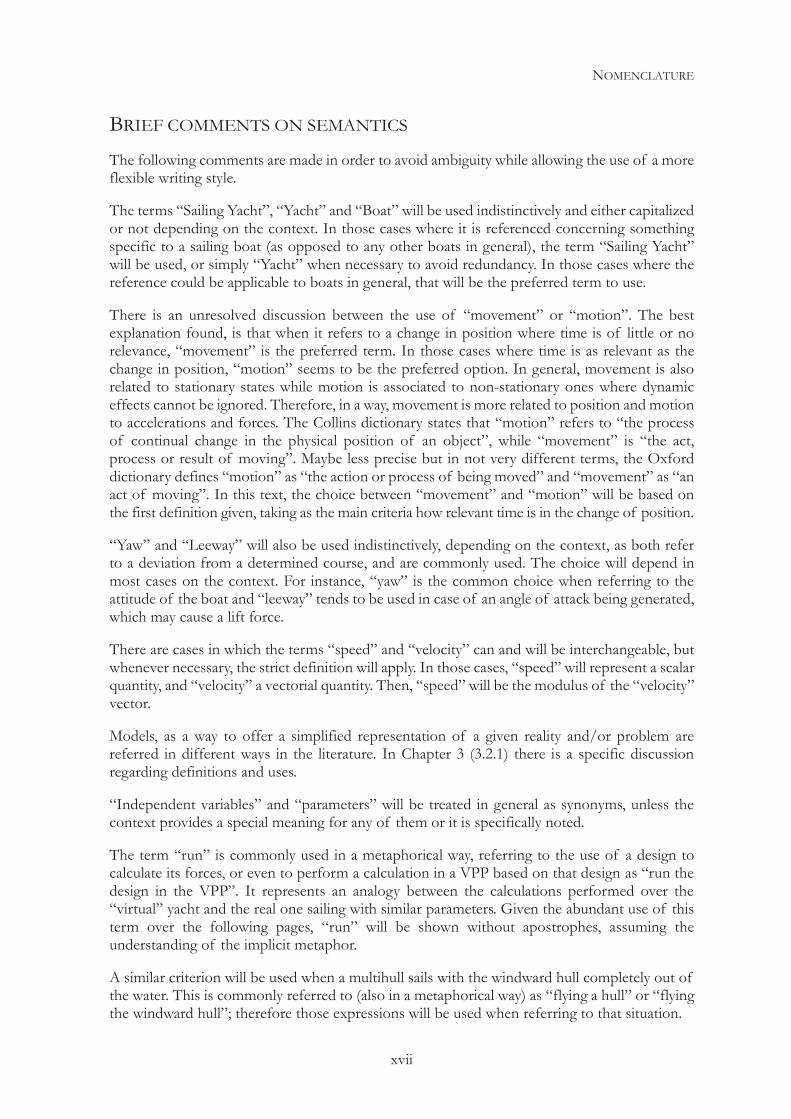
BRIEF COMMENTS ON SEMANTICS The following comments are made in order to avoid ambiguity while allowing the use of a more flexible writing style.
The terms “Sailing Yacht”, “Yacht” and “Boat” will be used indistinctively and either capitalized or not depending on the context. In those cases where it is referenced concerning something specific to a sailing boat (as opposed to any other boats in general), the term “Sailing Yacht” will be used, or simply “Yacht” when necessary to avoid redundancy. In those cases where the reference could be applicable to boats in general, that will be the preferred term to use.
There is an unresolved discussion between the use of “movement” or “motion”. The best explanation found, is that when it refers to a change in position where time is of little or no relevance, “movement” is the preferred term. In those cases where time is as relevant as the change in position, “motion” seems to be the preferred option. In general, movement is also related to stationary states while motion is associated to non-stationary ones where dynamic effects cannot be ignored. Therefore, in a way, movement is more related to position and motion to accelerations and forces. The Collins dictionary states that “motion” refers to “the process of continual change in the physical position of an object”, while “movement” is “the act, process or result of moving”. Maybe less precise but in not very different terms, the Oxford dictionary defines “motion” as “the action or process of being moved” and “movement” as “an act of moving”. In this text, the choice between “movement” and “motion” will be based on the first definition given, taking as the main criteria how relevant time is in the change of position.
“Yaw” and “Leeway” will also be used indistinctively, depending on the context, as both refer to a deviation from a determined course, and are commonly used. The choice will depend in most cases on the context. For instance, “yaw” is the common choice when referring to the attitude of the boat and “leeway” tends to be used in case of an angle of attack being generated, which may cause a lift force.
There are cases in which the terms “speed” and “velocity” can and will be interchangeable, but whenever necessary, the strict definition will apply. In those cases, “speed” will represent a scalar quantity, and “velocity” a vectorial quantity. Then, “speed” will be the modulus of the “velocity” vector.
Models, as a way to offer a simplified representation of a given reality and/or problem are referred in different ways in the literature. In Chapter 3 (3.2.1) there is a specific discussion regarding definitions and uses.
“Independent variables” and “parameters” will be treated in general as synonyms, unless the context provides a special meaning for any of them or it is specifically noted.
The term “run” is commonly used in a metaphorical way, referring to the use of a design to calculate its forces, or even to perform a calculation in a VPP based on that design as “run the design in the VPP”. It represents an analogy between the calculations performed over the “virtual” yacht and the real one sailing with similar parameters. Given the abundant use of this term over the following pages, “run” will be shown without apostrophes, assuming the understanding of the implicit metaphor.
A similar criterion will be used when a multihull sails with the windward hull completely out of the water. This is commonly referred to (also in a metaphorical way) as “flying a hull” or “flying the windward hull”; therefore those expressions will be used when referring to that situation.

NOMENCLATURE
xviii
This page intentionally left blank
OVERVIEW
1
1| OVERVIEW The assessment of performance for Sailing Yachts has been a problem under scientific consideration since Professor Kenneth S. M. Davison made a detailed explanation and analysis of the forces and moments involved in the equilibrium of Sailing Yachts in his paper from 1936 “Some Experimental Studies of the Sailing Yacht” (1). This paper was the result of a research program that involved testing scale models of Sailing Yachts in a towing tank.
Moreover, he went one step further and started to make a very innovative use at the time of his proposed test procedures. He collected data, which provided the base of the first actual scientific method to estimate the performance of a sailing yacht, in the stationary condition, which will happen at a point of equilibrium for a given set of wind conditions.
That equilibrium could happen under different sets of parameters and adjustments, and it is the search of those that becomes the focus of performance prediction for this type of boats, providing an optimal solution for performance (measured as the yacht speed or its projection on the Wind Axes).
The advent of computers in the ‘70s created an opportunity to develop the first actual performance prediction program (VPP). This happened through the H. Irving Pratt Ocean Racing Handicapping project at the Massachusetts Institute of Technology (MIT), that had its conclusions published at the Chesapeake Sailing Yacht Symposium in 1979 (2).
Before that, naval architects were limited to estimating equilibrium situations based on very simplified data with little margin for systematic optimization, which could be analyzed only in a limited way beyond their educated guesses.
Since then, computational resources have developed dramatically, making the use of VPPs a common tool for yacht designers. In addition, the requirements in terms of accuracy and flexibility have increased, along with the complexity of the type of yachts and problems to be analyzed.
This thesis intends to provide a generalized approach to performance prediction, taking into consideration the many aspects involved in achieving that objective, and their potential influence on the final result.
PROBLEM DEFINITION The basic problem for Sailing Yachts performance assessment starts with the definition of the state of equilibrium of a solid, subject to forces and moments generated by the action of the air and water over its surfaces (hull, sails, appendages, etc.).
These forces and moments are influenced and/or created by the movement of the Yacht, even when sailing in a stationary state. This brings the concept of apparent wind as the main definer for the forces of aerodynamic origin. In absence of current or waves, the sole movement of the boat provides the apparent water movement.
Via fundamentally the trim of the sails (but also by adjusting other parameters, which affect the hydrodynamic performance), it is possible to reach points of equilibrium which would happen
OVERVIEW
2
for each set of parameters, some of them independent, as wind angle and speed, and some others dependent. One of those parameters, the Yacht Speed (Vs) will be the main characterizer of performance, along with its projection over the wind axis, or velocity made good (VMG). VMG will allow estimating the optimal progression of the yacht against or towards the wind, for those situations in which the speed by itself becomes insufficient to assess performance.
Finding the sets of parameters that provide solutions for variations of true wind speed (TWS) and true wind angle (TWA) will allow unveiling the potential performance of a given Yacht. Therefore, the search of those combinations becomes the main purpose of the so-called Velocity Prediction Programs or VPPs.
Moving forward, the next step to consider is whether a calculated optimal solution is actually achievable by the Yacht using its own means. This would usually be the case with conventional displacement boats but it becomes more uncertain at high speeds when planing or foiling is involved and it may require a confirmation performing a time-domain analysis.
BACKGROUND AND CONTEXT. STATE OF THE ART Beyond the already mentioned initial studies from Professor Davison in his 1936 paper (1), it was in the late ‘70s that under the auspices of Commodore H. Irving Pratt researchers at the Massachusetts Institute of Technology were funded to produce a methodology that would predict the speed of a Sailing Yacht, based on its characteristics and wind conditions.
The H. Irving Pratt Ocean Racing Handicapping project produced the first Velocity Prediction Program (VPP), and covered a huge amount of new ground including:
A hydrodynamic force model based on towing tank tests.
An aerodynamic model for the sail forces at all relevant apparent wind angles.
Development of an iterative optimization scheme, which produced equilibrium sailing conditions.
Derivation of new methods of race scoring, to utilize the handicaps (normally defined as speeds expressed in seconds/mile) that the VPP predicted for each point of sailing.
Development of a hull offset measurement machine, and associate Lines Processing Program (LPP) to process hull shapes prior to introduction into the VPP.
This became the original Measurement Handicap System (MHS), which would eventually evolve into the International Measurement System (IMS) a few years later, when the Offshore Racing Council (ORC) decided to adopt it as its handicap system.
However, the most relevant outcome from that project related to this thesis, was its VPP, which provided the first real tool to predict the performance of sailing yachts. That VPP, originally adopted as the core of the IMS, has been maintained and further developed over more than two decades by the International Technical Committee (ITC) of the ORC.
Justin E. Kerwin, a prominent member of the original Pratt Project described the principles behind that first VPP in his article from 1978 “A velocity prediction program for ocean racing yachts” (3).
OVERVIEW
3
This original code was relatively simple, based on basic analytical models, and seriously restricted in the degrees of freedom (DOF) in which it could be solved. It is important to remember that the available computational resources at the time were a significant limitation, and that had an impact on what could be calculated.
The most basic solution of a VPP limited the calculation to a steady state equilibrium in Roll (Mx) and Surge (Fx). The equilibrium in the other degrees of freedom was assumed, and the effect on other variables of how it happened was ignored (for instance, the effect of the trim angle at which this equilibrium might occur is not taken into consideration for any further calculations).
This is in most cases a valid simplification, which covers the main part of the problem, and provides accurate enough results while simplifying the computational requirements. For that reason, it has been widely used for conventional monohulls and remains the core of the VPP used in the IMS.
Following the steps of Kerwin’s initial effort, different VPP tools have been developed over the years, helping to expand in different ways the capabilities of the original code. Some have emerged as commercial solutions for yachts designers, and many others, the most advanced ones, remain as proprietary codes, given the strategic importance of these tools, commonly used in high performance projects.
Faster boats, multihulls and in the limit hydrofoil supported Sailing Yachts involve additional complexities which make more difficult (if not impossible) to ignore equilibrium in other degrees of freedom and their coupled effects.
Also, the desire to analyze the problem in the time domain (some stationary states can be possible but without the guarantee of the existence of a valid path to reach them) have created a need to find ways to solve in other degrees of freedom. In many cases, this is done by making assumptions such as, for instance, a constant trim (or ignoring the effects of its change in order to eliminate coupling).
Similarly, a full consideration of the yacht’s motions requires a proper calculation of their effects on the incoming flow speed/direction. The introduction of non-stationary motions, and time as a variable, leads to the need to solve the differential equations rather than just a system of non-linear equations.
SCOPE The main objective of this thesis is to propose a generalized VPP model, along with a methodology and a computational tool, able to deal with any situation that could be considered for different types of sources of data, types of yachts or sailing modes. The final objective is to do this not just in a stationary state, but also to provide a path to perform time-domain analyses and simulations
Solutions will be provided for associated problems, along with guidelines for an efficient, robust and reliable, yet flexible process. Most of them will be implemented in a computational tool for performance analysis, in a broad interpretation of what that involves.
In order to achieve that, the aim is to:
OVERVIEW
4
Define a main framework, with a problem definition involving the six degrees of freedom and unrestricted soft and hard coupling.
Provide a methodology to obtain and process data in an efficient way adapted to the available resources, optimizing the use of them.
Establish different scenarios for which different parameters or degrees of freedom can be controlled indistinctively via physical and/or user-defined constraints.
Allow for a flexible use of constraints for specific parametric studies, providing a solver/optimize structure, which would permit different ways to solve the equilibrium.
Define the concept of “autopilots” as a way to incorporate criteria for managing constraints, in order to provide optimal yet realistic solution paths for time-domain analyses. This type of analysis would also be used as a mechanism to assess the feasibility of stationary solutions, as well as to optimize the transients between different stationary equilibrium sailing points.
Evaluate and integrate different solver/optimization strategies for the mathematical search of the equilibrium and optimal solutions, providing a computationally efficient process to facilitate the achievement of the previous objectives.
Compile the set of models, constrains, autopilots, rules and solving tools as a generic global yacht meta-model, which define the framework used to analyze the behavior of the sailing yacht and assess its performance.
Generate an object oriented computational tool named PASim (Performance Assessment Simulator) as the software implementation of the global yacht meta-model. This tool would integrate, amongst others features, a user interface and capabilities for an automated execution/interaction with external tools, for studies of a wider scope
Establish procedures for the conventional use of the tool, but also propose innovative uses such as feasibility studies for stationary cases, and or analyses of collected full-scale sailing data in a non-stationary environment.
Establish PASim as the engine for a sailing simulator, which would make use of the available sailing controls for a range of different yachts. This simulator would have as its main objectives to facilitate the sailor/designer interaction in high performance projects, as well as to verify the feasibility of optimal solutions from the operational point of view.
CONTRIBUTIONS The initial and base contribution of this research is a generalized definition of the equilibrium and motions of a sailing yacht and its constraints in a way that:
Provides full control for solving the equilibrium with six degrees of freedom, including the possibility to restrict and/or simplify the problem to adapt its solution to different types of analysis (ranging from a simple performance prediction to parametric studies
OVERVIEW
5
with partial optimization, including the possibility to lock state variables as additional constraints).
Establishes handles (autopilots) to restrict those degrees of freedom and/or manage the constraints for either a stationary or a time-domain analysis.
Has the ability to reproduce actual trimming procedures and reactions performed by sailors as closely to reality as possible, in an intuitive way, and allowing to test different trimming strategies in a time-domain calculation.
In addition to the above, a methodology has been developed to:
Plan experiments to collect data as the main source for the calculations of forces for predicting the performance of a sailing yacht.
Manage the acquired data in order to make the best possible use of it for that purpose.
Establish the different alternatives to solve the equilibrium (in a stationary state) and/or motions (in the time domain) of the yacht, proposing different solving/optimization techniques based on common definitions.
These definitions, models, rules and procedures will altogether conform a global yacht meta-model, as the definition of an abstraction of the real yacht, composed of the best knowledge available with the purpose of describing its behavior.
This is eventually integrated in a program that makes use of the discussed definitions and methodologies in order to perform performance predictions over a wide range of yachts and situations.
Some examples will illustrate conventional and non-conventional uses of the tool at the end of this research.
To summarize, the performance prediction of a sailing yacht is fundamentally a simple task with innumerable details that if not treated/handled properly could render the results useless. The purpose of this thesis is to provide the required critical insight into the problem, in order to offer a complete global vision, reflected in the global yacht meta-model, while raising awareness over the importance of some critical details.
OUTLINE OF THIS THESIS In order to achieve the objective of this research, the thesis is structured as follows.
In Chapter 2, the full definition of the problem is outlined, starting from the description of the equilibrium of a sailing yacht, to follow with the original solution proposed by Kerwin in 1978 (3), and extending that to the full problem involving the six degrees of freedom.
This is done by defining the sailing yacht movements, the concepts related to relative movement, such as the apparent velocities and angles, along with the influence of the relative movement on the propulsion, and by describing the forces and moments involved. It will also include an initial explanation about the origin of those forces and moments, and their couplings in the different degrees of freedom.
OVERVIEW
6
In Chapter 3, the origin of forces from static as well as aero and hydrodynamic origin is presented. After that, parametrization is briefly discussed, before talking about the generation and use of analytical models to estimate the forces and moments and about strategies regarding its use.
Chapter 4 analyzes the problem of obtaining data for performance prediction by using experimental and numerical analyses. This is structured with a starting point of planning the experiments to collect the required data, and then a more detailed discussion regarding the use of the experimental and numerical methods for obtaining data to use in a VPP. That discussion includes proposals for strategies to do this in an efficient and accurate way.
Chapter 5 deals with the management of data for and inside the VPP. It covers aspects ranging from the design of experiments to obtain that data, to the data calculation matrices and the interpolation for its use during calculations. This involves discussing accuracy and efficiency issues. A proposal is presented to generate and derive data from reduced sets of data
Chapter 6 starts with discussing variables and constraints, both of them with origin in the physics of sailing and in the normal operation of the yacht itself. It also introduces the concept of autopilots to manage those constraints. The main purpose of the generalized constraint management is to be able, as a first step, to obtain solutions with a conventional stationary-state equilibrium, and to define different specific types of analyses.
Then, the stationary solution of the problem is discussed, considering strategies to find the equilibrium for a given set of parameters, which could be optimized and manually adjusted in order to maximize an objective function.
Finally, the problem in the time domain is defined, evaluating a number of different approaches depending on the purpose of the study. Such approaches include analyzing the evolution of equilibrium with stable wind and fixed adjustments, or trying to obtain the adjustments for an optimal acceleration path or analyzing the feasibility of previously calculated optima for a stationary-state solution.
Chapter 7 describes the specification and structure of the performance prediction tool (computer program) in its definition, control and solution, and describes its interaction with external modules.
Chapter 8 shows examples of solutions to different problems related to performance prediction, that could be considered a conventional use of VPP, in order to illustrate some of the points discussed before. They include a traditional solution of a VPP and specific studies in more challenging conditions (such as the use of data from different origins, multiple optima, multi-parametric optimizations time-domain analyses).
Chapter 9 describes less conventional examples of performance assessment, including the use of the VPP in global multi-parametric optimization studies, or the time-domain analyses between different optimum sailing points. It also proposes procedures to use PaSim to improve the analysis of full scale collected sailing data, which because of the usual conditions of variability in the environment, are extremely difficult to evaluate.
Chapter 10 summarizes the core of the work in this thesis in a global yacht meta-model as a general framework for performance assessment, applicable to different problems and types of analyses or yachts. It also proposes the use of this meta-model, through PASim, as the engine for a physical sailing simulator, including a simplified specification and description of the whole
OVERVIEW
7
system. This involves a movable platform to reproduce motions and accelerations, physical controls, and integration with virtual reality tools in order to provide a realistic experience for designers and sailors.
Finally, Chapter 11 outlines conclusions of this research, proposing specific lines of investigation to complement and further extend the scope of this thesis.
A NOTE ON THIS THESIS APPROACH TO THE PROBLEM The object of this research involves a high number of different fields of engineering and science in general, for which significant developments are available. In most cases they require the use of specialized mathematical resources and tools, that bring along the risk of making too much of an abstraction in detriment of a more conceptual discussion.
This is fundamentally an engineering thesis as opposed to one based on fundamental science; therefore, notwithstanding the obvious need to rely on that science for the solution of the problems, a conscious decision is made to focus more on the physics of it, the concept, rather than on the mathematics, the language.
A number of examples can be given regarding this choice. For instance, lift around an airfoil can be explained in terms of circulation, but also as a consequence of the altered field of pressures around it. Both explanations are true and reflect the same physical phenomena, but the latter provides a more intuitive explanation of how the forces are generated, than the former explanation.
Similarly, some mathematical transformations may facilitate the solution of some equations with specific simplifications, but opting for a numerical solution may preserve a generalized approach and a better perception of the solution process, even if it may happen at the expense of a more time-consuming calculation.
The purpose of these comments is not to detract from the use or research of whichever available mathematical tools may be available, but rather to preserve the value of the concept and the actual physical phenomena involved.
The main objective is to provide a good general vision of the global problem. This will allow the engineer to make conscious and informed decisions regarding the methods, simplifications and, in general, the modelling and calculation strategies for the assessment of yacht performance, a process affected by a large number of factors, often interdependent.

OVERVIEW
8
This page intentionally left blank
DESCRIPTION OF THE PROBLEM
9
2| DESCRIPTION OF THE PROBLEM The motions of a Sailing Yacht play a critical role in its performance. This happens even to a bigger extent than in other types of boats, given the nature of the propulsion system, which turns the relative wind into the key element for the creation of the driving force.
Besides, the sailing yacht encounters an always-changing environment in terms of wind and waves, which induce additional motions to a greater or lesser extent in all six degrees of freedom.
Even when sailing in a stationary situation, it is necessary to take into account the effects of the relative movement in the definition of the wind conditions. In addition, when sailing in non-stationary states, the motions add a layer of changes that need to be taken into account when solving the problem in the time domain.
This process needs to start by describing the basic aspects of the geometry of sailing in a stationary state, the factors involved in that equilibrium and the definitions necessary to grab a good understanding of the underlying physics and the strategy to solve the related problems. This will be the main purpose of this Chapter.
GEOMETRY OF SAILING AND APPARENT WIND One fundamental concept related to sail propulsion is the apparent wind, result of composing the true wind (the actual wind measured by a static observer) with the wind generated by the Yacht’s movement.
Although later in this Chapter there will be a brief discussion regarding the wind gradient with height, in general the wind will be characterized by the modulus and direction of the vector defining it within the horizontal plane parallel to the water surface. That is, by the wind speed and wind angle.
The simplest possible definition of apparent wind is the one that can be made in absence of any true wind (total calm), when a moving observer experiences a wind with a velocity equal to his moving velocity and opposed in direction to his own movement. Including an existent wind with a given velocity and relative angle will simply add an additional vectorial component that, when combined with the one generated by the movement, will determine the resultant wind as measured in the moving system of reference. This will be the apparent wind as perceived by the moving observer.
The next natural step is to extend this concept to a sailing yacht in a standard upwind sailing situation. In this case, the boat will follow a course at an angle with the wind axis of less than 90 degrees. The described vector composition provides the key elements necessary to define the apparent wind that the yacht will “see”, this time adding an angle between the direction of the existing wind and the movement of the yacht.
A number of authors ( (4), (5), (6)) have described this, in what is called “theory of sailing” and provided slightly different views of the same situation. That also introduces the definition of VMG (velocity made good to windward/leeward) as the projection of the yacht velocity vector over the wind axis.
DESCRIPTION OF THE PROBLEM
10
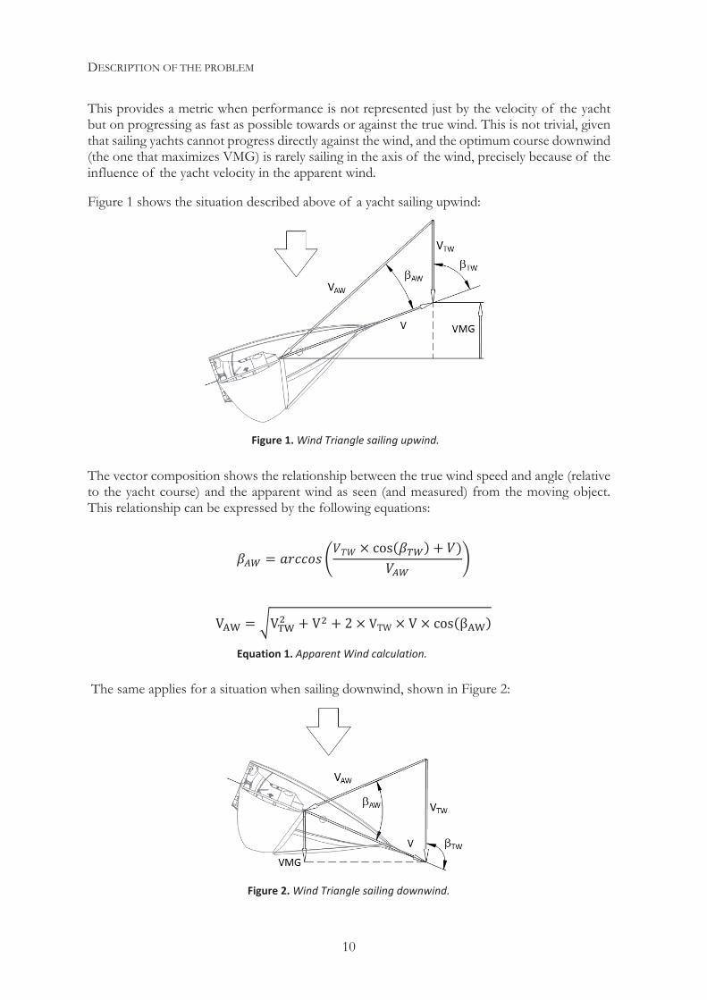
This provides a metric when performance is not represented just by the velocity of the yacht but on progressing as fast as possible towards or against the true wind. This is not trivial, given that sailing yachts cannot progress directly against the wind, and the optimum course downwind (the one that maximizes VMG) is rarely sailing in the axis of the wind, precisely because of the influence of the yacht velocity in the apparent wind.
Figure 1 shows the situation described above of a yacht sailing upwind:
The vector composition shows the relationship between the true wind speed and angle (relative to the yacht course) and the apparent wind as seen (and measured) from the moving object. This relationship can be expressed by the following equations:
The same applies for a situation when sailing downwind, shown in Figure 2:
Figure 1. Wind Triangle sailing upwind.
Equation 1. Apparent Wind calculation.
Figure 2. Wind Triangle sailing downwind.
DESCRIPTION OF THE PROBLEM
11
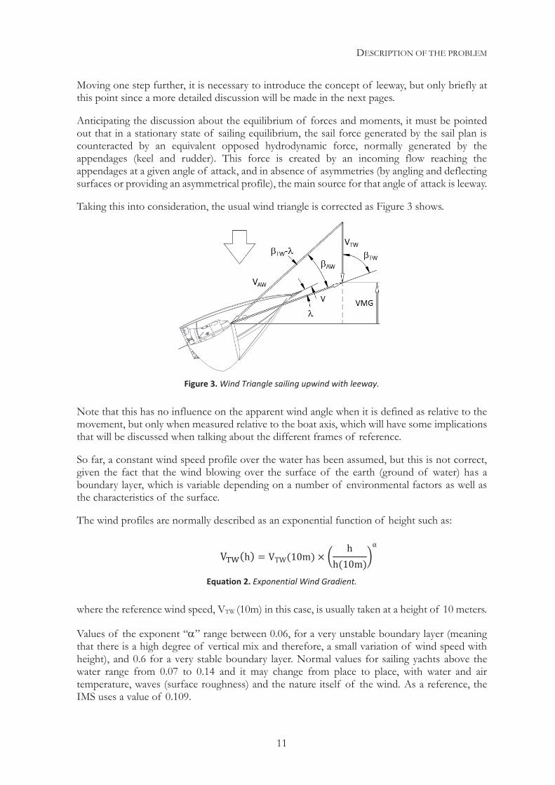
Moving one step further, it is necessary to introduce the concept of leeway, but only briefly at this point since a more detailed discussion will be made in the next pages.
Anticipating the discussion about the equilibrium of forces and moments, it must be pointed out that in a stationary state of sailing equilibrium, the sail force generated by the sail plan is counteracted by an equivalent opposed hydrodynamic force, normally generated by the appendages (keel and rudder). This force is created by an incoming flow reaching the appendages at a given angle of attack, and in absence of asymmetries (by angling and deflecting surfaces or providing an asymmetrical profile), the main source for that angle of attack is leeway.
Taking this into consideration, the usual wind triangle is corrected as Figure 3 shows.
Note that this has no influence on the apparent wind angle when it is defined as relative to the movement, but only when measured relative to the boat axis, which will have some implications that will be discussed when talking about the different frames of reference.
So far, a constant wind speed profile over the water has been assumed, but this is not correct, given the fact that the wind blowing over the surface of the earth (ground of water) has a boundary layer, which is variable depending on a number of environmental factors as well as the characteristics of the surface.
The wind profiles are normally described as an exponential function of height such as:
where the reference wind speed, VTW (10m) in this case, is usually taken at a height of 10 meters.
Values of the exponent “ ” range between 0.06, for a very unstable boundary layer (meaning that there is a high degree of vertical mix and therefore, a small variation of wind speed with height), and 0.6 for a very stable boundary layer. Normal values for sailing yachts above the water range from 0.07 to 0.14 and it may change from place to place, with water and air temperature, waves (surface roughness) and the nature itself of the wind. As a reference, the IMS uses a value of 0.109.
Figure 3. Wind Triangle sailing upwind with leeway.
Equation 2. Exponential Wind Gradient.
DESCRIPTION OF THE PROBLEM
12
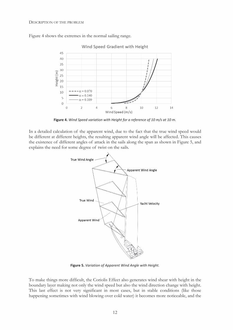
Figure 4 shows the extremes in the normal sailing range.
In a detailed calculation of the apparent wind, due to the fact that the true wind speed would be different at different heights, the resulting apparent wind angle will be affected. This causes the existence of different angles of attack in the sails along the span as shown in Figure 5, and explains the need for some degree of twist on the sails.
To make things more difficult, the Coriolis Effect also generates wind shear with height in the boundary layer making not only the wind speed but also the wind direction change with height. This last effect is not very significant in most cases, but in stable conditions (like those happening sometimes with wind blowing over cold water) it becomes more noticeable, and the
Figure 4. Wind Speed variation with Height for a reference of 10 m/s at 10 m.
Figure 5. Variation of Apparent Wind Angle with Height.
DESCRIPTION OF THE PROBLEM
13
sails start requiring to be trimmed with a more significant difference in twist from tack to tack in order to adapt to this circumstance.
All this can, and in most cases, must be taken into account in detailed sail studies. However, in the majority of the sail models used in VPPs, it is normal to estimate a resultant wind in the center of effort of the sail for a given wind profile. This is defined by a nominal wind speed at a height of 10 meters, which can be tuned for different conditions in a more or less detailed way. In most cases this is not an oversimplification, since the source of data used to build the sail models has been obtained considering the existence of some wind gradient.
The level of detail of the VPP sail models can range from a simple center of effort calculation based on area, corrected or not by gradient to a more detailed aerodynamic model which takes into consideration all the effects. This way, for instance, the span-wise lift distribution, along with its impact on lift and drag of the sail plan and therefore on the driving force, heeling moment etc., can be properly evaluated.
The simplest acceptable correction, for a proper calculation is to solve the wind triangle with the value of TWS estimated for the height at which the center of effort of the sail plan is expected to be, based on the center of the sail area and the nominal wind speed for a reference height (normally 10 meters).
In the last years, in highly competitive events (where more resources are available), we have seen an increase in teams trying to measure a more or less detailed wind profile to incorporate corrections according to it.
These corrections range from adjusting target values to the analysis of collected full-scale data; therefore, it is certainly something to be taken into account related to performance prediction. However, it belongs more to the physics of the aerodynamic calculations than to the procedures related to performance prediction per-se, so we will not go into a more detailed discussion here.
SYSTEMS OF REFERENCE. SETS OF AXES When studying and calculating the equilibrium of a moving object, it becomes convenient the use of different systems of reference. This is reinforced by the fact that in our case the moving object operates within two different fluids, which have a different relative movement to them, so there will be different directions and speeds for the water and air incoming flows.
During the study of equilibrium, different systems of reference will be used for the calculations of forces of different origin, and they will ultimately be referred to one common system, to compare, balance or evaluate the equilibrium.
There is little dispute regarding which are the relevant systems of reference when studying the physics of a sailing yacht, but there is less agreement regarding the nomenclature. The ones used here are similar to those proposed by A.R. Claughton in “Sailing Yacht Design” (7).
The systems of reference will be defined by different sets of right hand orthogonal axes.
It seems reasonable to start defining a set of Boat Axes in the traditional way naval architecture does. Assuming the yacht in an arbitrary flotation in calm water the X-Y plane will be defined in that flotation plane, with the X-axis extending longitudinally in the centerline plane and the
DESCRIPTION OF THE PROBLEM
14
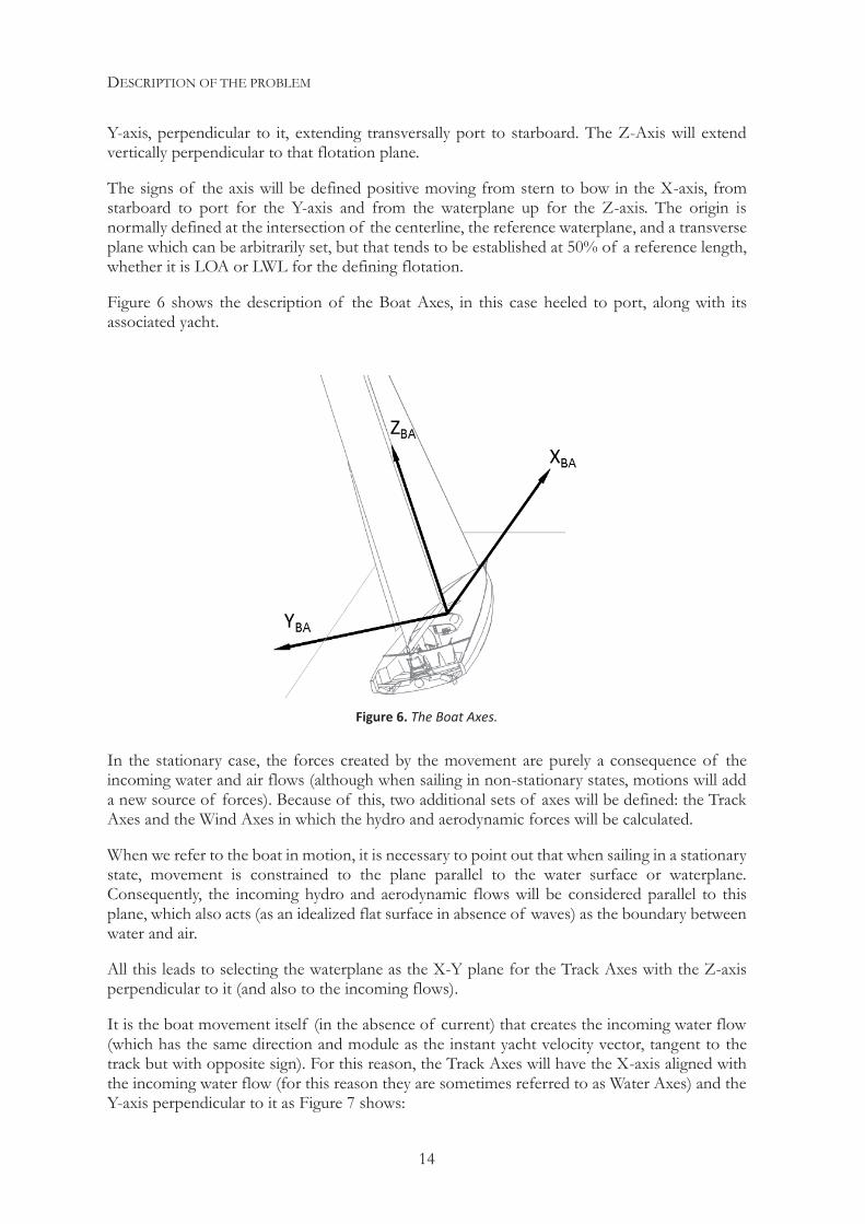
Y-axis, perpendicular to it, extending transversally port to starboard. The Z-Axis will extend vertically perpendicular to that flotation plane.
The signs of the axis will be defined positive moving from stern to bow in the X-axis, from starboard to port for the Y-axis and from the waterplane up for the Z-axis. The origin is normally defined at the intersection of the centerline, the reference waterplane, and a transverse plane which can be arbitrarily set, but that tends to be established at 50% of a reference length, whether it is LOA or LWL for the defining flotation.
Figure 6 shows the description of the Boat Axes, in this case heeled to port, along with its associated yacht.
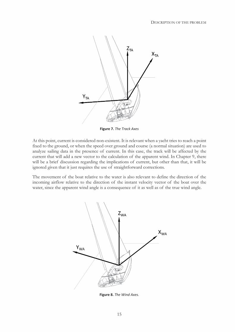
In the stationary case, the forces created by the movement are purely a consequence of the incoming water and air flows (although when sailing in non-stationary states, motions will add a new source of forces). Because of this, two additional sets of axes will be defined: the Track Axes and the Wind Axes in which the hydro and aerodynamic forces will be calculated.
When we refer to the boat in motion, it is necessary to point out that when sailing in a stationary state, movement is constrained to the plane parallel to the water surface or waterplane. Consequently, the incoming hydro and aerodynamic flows will be considered parallel to this plane, which also acts (as an idealized flat surface in absence of waves) as the boundary between water and air.
All this leads to selecting the waterplane as the X-Y plane for the Track Axes with the Z-axis perpendicular to it (and also to the incoming flows).
It is the boat movement itself (in the absence of current) that creates the incoming water flow (which has the same direction and module as the instant yacht velocity vector, tangent to the track but with opposite sign). For this reason, the Track Axes will have the X-axis aligned with the incoming water flow (for this reason they are sometimes referred to as Water Axes) and the Y-axis perpendicular to it as Figure 7 shows:
Figure 6. The Boat Axes.
DESCRIPTION OF THE PROBLEM
15
At this point, current is considered non-existent. It is relevant when a yacht tries to reach a point fixed to the ground, or when the speed over ground and course (a normal situation) are used to analyze sailing data in the presence of current. In this case, the track will be affected by the current that will add a new vector to the calculation of the apparent wind. In Chapter 9, there will be a brief discussion regarding the implications of current, but other than that, it will be ignored given that it just requires the use of straightforward corrections.
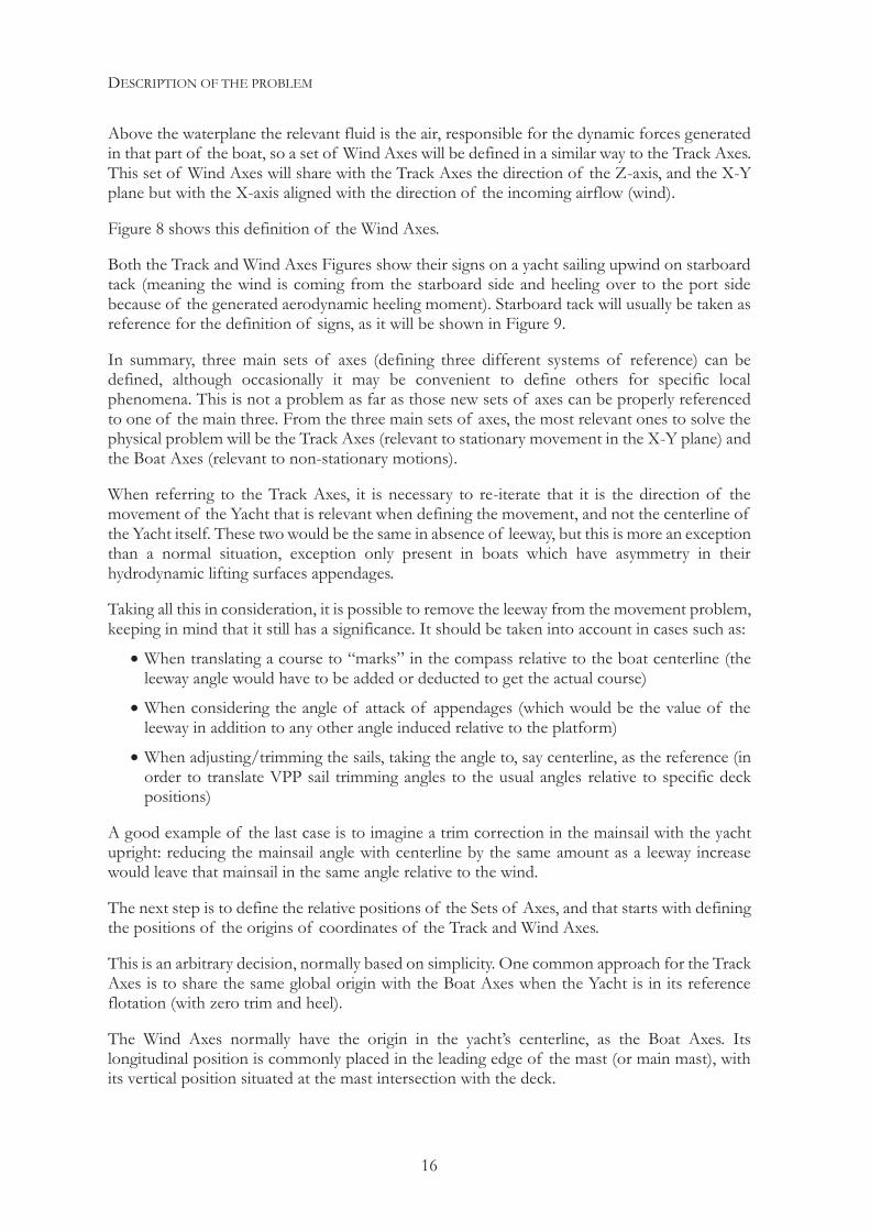
The movement of the boat relative to the water is also relevant to define the direction of the incoming airflow relative to the direction of the instant velocity vector of the boat over the water, since the apparent wind angle is a consequence of it as well as of the true wind angle.
Figure 7. The Track Axes
Figure 8. The Wind Axes.
DESCRIPTION OF THE PROBLEM
16
Above the waterplane the relevant fluid is the air, responsible for the dynamic forces generated in that part of the boat, so a set of Wind Axes will be defined in a similar way to the Track Axes. This set of Wind Axes will share with the Track Axes the direction of the Z-axis, and the X-Y plane but with the X-axis aligned with the direction of the incoming airflow (wind).
Figure 8 shows this definition of the Wind Axes.
Both the Track and Wind Axes Figures show their signs on a yacht sailing upwind on starboard tack (meaning the wind is coming from the starboard side and heeling over to the port side because of the generated aerodynamic heeling moment). Starboard tack will usually be taken as reference for the definition of signs, as it will be shown in Figure 9.
In summary, three main sets of axes (defining three different systems of reference) can be defined, although occasionally it may be convenient to define others for specific local phenomena. This is not a problem as far as those new sets of axes can be properly referenced to one of the main three. From the three main sets of axes, the most relevant ones to solve the physical problem will be the Track Axes (relevant to stationary movement in the X-Y plane) and the Boat Axes (relevant to non-stationary motions).
When referring to the Track Axes, it is necessary to re-iterate that it is the direction of the movement of the Yacht that is relevant when defining the movement, and not the centerline of the Yacht itself. These two would be the same in absence of leeway, but this is more an exception than a normal situation, exception only present in boats which have asymmetry in their hydrodynamic lifting surfaces appendages.
Taking all this in consideration, it is possible to remove the leeway from the movement problem, keeping in mind that it still has a significance. It should be taken into account in cases such as:
When translating a course to “marks” in the compass relative to the boat centerline (the leeway angle would have to be added or deducted to get the actual course)
When considering the angle of attack of appendages (which would be the value of the leeway in addition to any other angle induced relative to the platform)
When adjusting/trimming the sails, taking the angle to, say centerline, as the reference (in order to translate VPP sail trimming angles to the usual angles relative to specific deck positions)
A good example of the last case is to imagine a trim correction in the mainsail with the yacht upright: reducing the mainsail angle with centerline by the same amount as a leeway increase would leave that mainsail in the same angle relative to the wind.
The next step is to define the relative positions of the Sets of Axes, and that starts with defining the positions of the origins of coordinates of the Track and Wind Axes.
This is an arbitrary decision, normally based on simplicity. One common approach for the Track Axes is to share the same global origin with the Boat Axes when the Yacht is in its reference flotation (with zero trim and heel).
The Wind Axes normally have the origin in the yacht’s centerline, as the Boat Axes. Its longitudinal position is commonly placed in the leading edge of the mast (or main mast), with its vertical position situated at the mast intersection with the deck.
DESCRIPTION OF THE PROBLEM
17
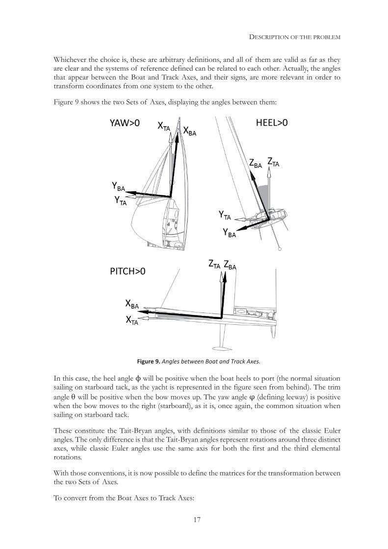
Whichever the choice is, these are arbitrary definitions, and all of them are valid as far as they are clear and the systems of reference defined can be related to each other. Actually, the angles that appear between the Boat and Track Axes, and their signs, are more relevant in order to transform coordinates from one system to the other.
Figure 9 shows the two Sets of Axes, displaying the angles between them:
In this case, the heel angle will be positive when the boat heels to port (the normal situation sailing on starboard tack, as the yacht is represented in the figure seen from behind). The trim angle will be positive when the bow moves up. The yaw angle (defining leeway) is positive when the bow moves to the right (starboard), as it is, once again, the common situation when sailing on starboard tack.
These constitute the Tait-Bryan angles, with definitions similar to those of the classic Euler angles. The only difference is that the Tait-Bryan angles represent rotations around three distinct axes, while classic Euler angles use the same axis for both the first and the third elemental rotations.
With those conventions, it is now possible to define the matrices for the transformation between the two Sets of Axes.
To convert from the Boat Axes to Track Axes:
Figure 9. Angles between Boat and Track Axes.
DESCRIPTION OF THE PROBLEM
18
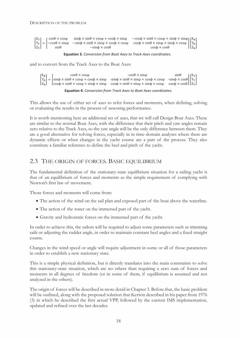
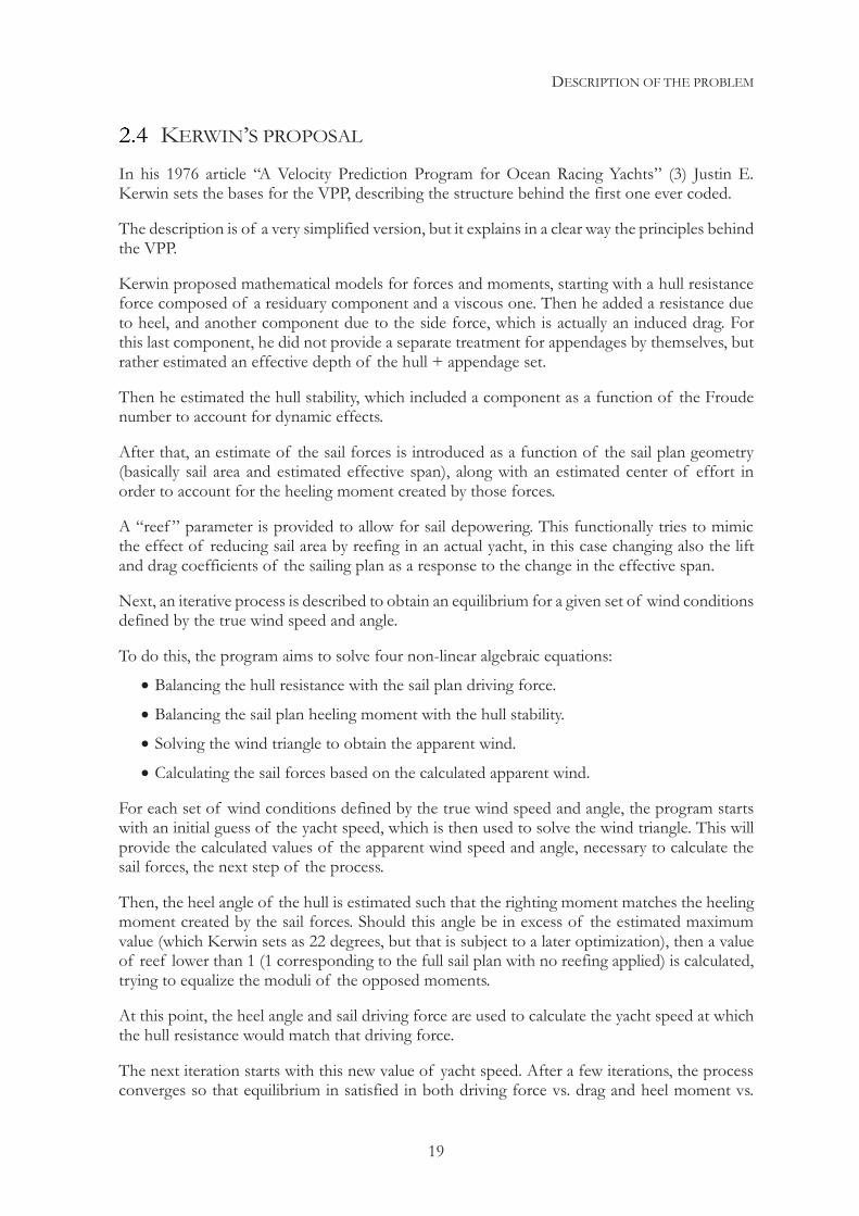
and to convert from the Track Axes to the Boat Axes:
This allows the use of either set of axes to refer forces and moments, when defining, solving or evaluating the results in the process of assessing performance.
It is worth mentioning here an additional set of axes, that we will call Design Boat Axes. These are similar to the normal Boat Axes, with the difference that their pitch and yaw angles remain zero relative to the Track Axes, so the yaw angle will be the only difference between them. They are a good alternative for solving forces, especially in in time-domain analyses where there are dynamic effects or when changes in the yacht course are a part of the process. They also constitute a familiar reference to define the heel and pitch of the yacht.
THE ORIGIN OF FORCES. BASIC EQUILIBRIUM The fundamental definition of the stationary-state equilibrium situation for a sailing yacht is that of an equilibrium of forces and moments as the simple requirement of complying with Newton’s first law of movement.
Those forces and moments will come from:
The action of the wind on the sail plan and exposed part of the boat above the waterline.
The action of the water on the immersed part of the yacht.
Gravity and hydrostatic forces on the immersed part of the yacht.
In order to achieve this, the sailors will be required to adjust some parameters such as trimming sails or adjusting the rudder angle, in order to maintain constant heel angles and a fixed straight course.
Changes in the wind speed or angle will require adjustment in some or all of those parameters in order to establish a new stationary state.
This is a simple physical definition, but it directly translates into the main constraints to solve this stationary-state situation, which are no others than requiring a zero sum of forces and moments in all degrees of freedom (or in some of them, if equilibrium is assumed and not analyzed in the others).
The origin of forces will be described in more detail in Chapter 3. Before that, the basic problem will be outlined, along with the proposed solution that Kerwin described in his paper from 1976 (3) in which he described the first actual VPP, followed by the current IMS implementation, updated and refined over the last decades.
Equation 3. Conversion from Boat Axes to Track Axes coordinates.
Equation 4. Conversion from Track Axes to Boat Axes coordinates.
DESCRIPTION OF THE PROBLEM
19
KERWIN’S PROPOSAL In his 1976 article “A Velocity Prediction Program for Ocean Racing Yachts” (3) Justin E. Kerwin sets the bases for the VPP, describing the structure behind the first one ever coded.
The description is of a very simplified version, but it explains in a clear way the principles behind the VPP.
Kerwin proposed mathematical models for forces and moments, starting with a hull resistance force composed of a residuary component and a viscous one. Then he added a resistance due to heel, and another component due to the side force, which is actually an induced drag. For this last component, he did not provide a separate treatment for appendages by themselves, but rather estimated an effective depth of the hull + appendage set.
Then he estimated the hull stability, which included a component as a function of the Froude number to account for dynamic effects.
After that, an estimate of the sail forces is introduced as a function of the sail plan geometry (basically sail area and estimated effective span), along with an estimated center of effort in order to account for the heeling moment created by those forces.
A “reef ” parameter is provided to allow for sail depowering. This functionally tries to mimic the effect of reducing sail area by reefing in an actual yacht, in this case changing also the lift and drag coefficients of the sailing plan as a response to the change in the effective span.
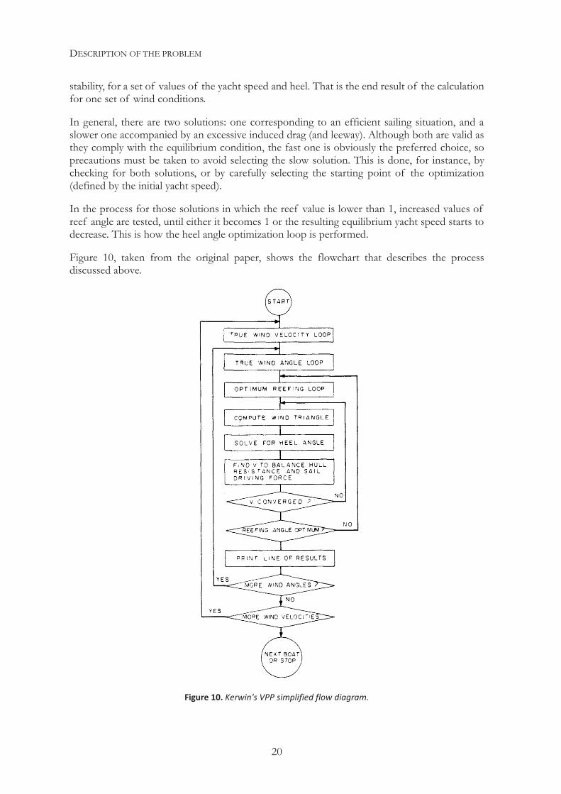
Next, an iterative process is described to obtain an equilibrium for a given set of wind conditions defined by the true wind speed and angle.
To do this, the program aims to solve four non-linear algebraic equations:
Balancing the hull resistance with the sail plan driving force.
Balancing the sail plan heeling moment with the hull stability.
Solving the wind triangle to obtain the apparent wind.
Calculating the sail forces based on the calculated apparent wind.
For each set of wind conditions defined by the true wind speed and angle, the program starts with an initial guess of the yacht speed, which is then used to solve the wind triangle. This will provide the calculated values of the apparent wind speed and angle, necessary to calculate the sail forces, the next step of the process.
Then, the heel angle of the hull is estimated such that the righting moment matches the heeling moment created by the sail forces. Should this angle be in excess of the estimated maximum value (which Kerwin sets as 22 degrees, but that is subject to a later optimization), then a value of reef lower than 1 (1 corresponding to the full sail plan with no reefing applied) is calculated, trying to equalize the moduli of the opposed moments.
At this point, the heel angle and sail driving force are used to calculate the yacht speed at which the hull resistance would match that driving force.
The next iteration starts with this new value of yacht speed. After a few iterations, the process converges so that equilibrium in satisfied in both driving force vs. drag and heel moment vs.
DESCRIPTION OF THE PROBLEM
20
stability, for a set of values of the yacht speed and heel. That is the end result of the calculation for one set of wind conditions.
In general, there are two solutions: one corresponding to an efficient sailing situation, and a slower one accompanied by an excessive induced drag (and leeway). Although both are valid as they comply with the equilibrium condition, the fast one is obviously the preferred choice, so precautions must be taken to avoid selecting the slow solution. This is done, for instance, by checking for both solutions, or by carefully selecting the starting point of the optimization (defined by the initial yacht speed).
In the process for those solutions in which the reef value is lower than 1, increased values of reef angle are tested, until either it becomes 1 or the resulting equilibrium yacht speed starts to decrease. This is how the heel angle optimization loop is performed.
Figure 10, taken from the original paper, shows the flowchart that describes the process discussed above.
Figure 10. Kerwin's VPP simplified flow diagram.
DESCRIPTION OF THE PROBLEM
21
THE IMS VPP After adopting the basic MHS in the mid 80’s as its core handicap system, the Offshore Racing Congress (ORC) has kept improving the VPP as well as the whole handicap system, which via the International Technical Committee (ITC) turned into the IMS, in use up until today. V of respected scientists and designers from all over the world, who have devoted volunteer work to this purpose, and continue doing so.
As can be expected, as a result the original concept has been greatly refined and improved since its original adoption. Moreover, in the last years, part of the work of the ITC has been dedicated to documenting the science behind the VPP and publishing it as parts of the rules of the handicap system (8). In addition, most of the source code of the VPP has been publicly available over the years. This has complemented the information already published in a few papers describing the IMS over the years ( (9), (10), (11), (12)).
All this documented information makes unnecessary to include a detailed description of the VPP itself here, but it is useful to mention to a few of the improvements incorporated over the original MHS.
On one hand, the VPP includes what is called a Lines Processing Program or LPP, which is nothing else than a program that performs hydrostatic and stability calculations using section offsets files. These files describe the geometry of the boat along with information regarding its weight and center of gravity, normally deduced from a full-scale flotation and stability experiment.
The LPP results include a number of conventional hydrostatic parameters (such as LWL, BWL, Wetted surfaces, etc.) as well as some specific parameters designed to facilitate the creation of accurate models to calculate the forces and moments involved in the equilibrium (such as effective weighted lengths or beams). It also performs a stability analysis with calculations of the variations of some of those parameters with heel.
With all that physical information about the Yacht, a Rig Analysis routine derives a “collective” set of sail coefficients from those corresponding to individual sails, and then it solves the equilibrium in the same two degrees of freedom that Kerwin considered.
A first change the IMS program introduced long ago was a depowering parameter called “flat”, in addition to the already mentioned “reef ”. “Flat” decreases the lift and drag coefficients without changing the effective span, trying to reproduce the process of using flatter sails or reducing their depth. “Reef ” and “flat” become two optimization variables, which act independently, so the model starts flattening sails until a specific limit is reached but it also starts reefing. Normally a combination of both produces the estimated optima.
In the last years, a depowering scheme which reproduced more faithfully the normal depowering sequence in offshore yachts was adopted. It takes a reefing approach for mainsails, and a jib foot length reduction for headsails, in addition to the flat parameter. This allows for consideration of variations in aspect ratio and effective span individually for each sail before calculating the “collective” coefficients.
This more detailed aerodynamic depowering scheme is accompanied by much more accurate and robust analytical models in any source of forces considered, both from hydrodynamic and aerodynamic origin. This is the result of a number of experimental tests (in towing tanks and
DESCRIPTION OF THE PROBLEM
22
wind tunnels), and lately CFD analyses, to either help to tune the existent analytical parametric models or create new more accurate ones based on the new collected data from experiments.
Since the main objective of the IMS VPP is to predict performance for a wide range of Yachts, the importance of the complexity (in terms of number of parameters being considered) and accuracy of these models is significant, although sometimes it creates type-forming problems.
This by itself would constitute material for a number of theses and it is always subject to improvements, whether the purpose is to specialize for a type of yachts or to provide a valid answer for a wide range of them (as is the task of a handicap system like IMS)..
The specific area of parametric models, one of the sources of data we will refer to in Chapter 3, is where the most effort has been applied to the IMS VPP. This is fundamentally an effort to improve the knowledge of the aero and hydrodynamic forces involved in the equilibrium of sailing yachts and the effect that the yacht characteristics have on those forces. This effect becomes the key of generalist performance prediction.
In addition, the equilibrium calculation and the optimization on the depowering parameters have evolved in the IMS VPP into an integrated solver/optimizer, which provides a more efficient solving technique in terms of computational requirements and stability.
SIX DEGREES OF FREEDOM Without getting here into a detailed discussion about the physics in Kerwin’s VPP (there is a good explanation of them in the original paper (3)), they provide a reasonably accurate description of the phenomena involved in the equilibrium of a sailing yacht via analytical models. However, these are very simplified, and limited in terms of degrees of freedom as well as the coupling between them.
This simplification is done by either ignoring movements in other axis or neglecting their effects. For instance, due to the sail induced pitch moment, there is a change in longitudinal trim of the boat, which is ignored. While this change in trim could be calculated as an output, its effects on drag for instance are neglected.
In many cases, this is not a problem since those influences are small, so deciding to ignore them was probably a wise decision at the time.
The parametric models behind the IMS VPP have dramatically improved the accuracy for forces and moments calculations, but a good part of the other limitations remain.
Also, when getting into more detailed calculations or less conventional analyses, these simplifications become a problem. A more complete definition is required, forcing to make a conscious decision on what to ignore and/or neglect, rather than just ignoring without any further consideration.
Therefore, the proposal in this thesis for a “general tool” is not to systematically overcomplicate the problem but rather to leave the door open for a complete unrestricted resolution. From that point, the intention is to encourage making every decision regarding simplifications with a full knowledge of their implications.
DESCRIPTION OF THE PROBLEM
23
At this point, it seems necessary to review the effects of forces and motions in the different degrees of freedom, the source of forces (broadly speaking, since this will be discussed in Chapter 3 with a higher level of detail), the moments they generate, and the possible coupling effects, for a generalized yacht.
This will start with describing the possible different motions, responsible for the changes in the position of the Yacht. After that, as mentioned above, it will be time to review in more detail the relationship between the forces and the moments due to those motions. All these aspects together will provide a full definition of the yacht in a complete six degrees of freedom “world”, as a starting point to study its movement.
2.6.1 MOTIONS
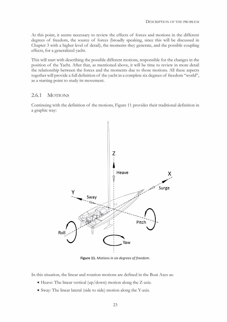
Continuing with the definition of the motions, Figure 11 provides their traditional definition in a graphic way:
In this situation, the linear and rotation motions are defined in the Boat Axes as:
Heave: The linear vertical (up/down) motion along the Z-axis.
Sway: The linear lateral (side to side) motion along the Y-axis.
Figure 11. Motions in six degrees of freedom.
DESCRIPTION OF THE PROBLEM
24
Surge: The linear longitudinal (front/back) motion along the X-axis.
Pitch: The rotation around the transverse (side to side) Y-axis. (The angle defining the position in this axis is referred to as “trim”)
Roll: The rotation around the longitudinal (front/back) X-axis. (The angle defining the position in this axis is referred to as “heel”)
Yaw: The rotation around the vertical (up/down) Z-axis. (The angle defining the position in this axis is referred to as “yaw”)
2.6.2 FORCES
The next step is to identify the origin of the forces (and moments they create) which are involved in the motions of the yacht. We will decompose them in the Track Axes, and point out the main contributors, the moments they create and the main types of coupling which happen between them.
At this stage, a stationary state of sailing will be assumed, and for that, there will be a requirement of equilibrium of forces and moments. However, when extending this to a dynamic solution of the problem, motions and accelerations will be caused by an imbalance. It is important to remember that the equilibrium is not a requirement for the boat sailing but for doing it in a stationary state as required by Newton’s laws.
In addition, it is necessary to point out that although some forces are dominantly in one axis or another (depending also on the system of reference, and for this exercise we will use the Track Axes system of reference), most of them have components in more than one axis. At this point, only the most significant components will be mentioned, with a purely descriptive intention rather than a more strict definition, which will be made in the next Chapter.
The figures describing an equilibrium situation will display forces, which generate a moment. Obviously, at that equilibrium, the moments will be balanced as well as the forces, but this will be used sometimes as a “drawing license” to suggest that there is one missing force, which will provide that missing moment balance when the boat sails in a stationary state.
In all cases, given the nature of forces involved and the two fluids in which a sailing yacht moves, there will be a resultant aerodynamic force and moment opposing to a resultant hydrodynamic force and moment.
Hydrodynamic forces are generated by the incoming water flow, created by the movement of the yacht in the direction of the X-axis of the Track Axes. They can be decomposed into a “drag” component along the X-axis and a “lift” component perpendicular to it, along the Y-axis. There may also be a Z-axis component, which we will call “vertical force”, and being perpendicular to the incoming flow it will also have a “lifting” nature.
Aerodynamic forces are similarly generated by the incoming airflow, created by the movement of the yacht in the X-axis of the Track Axes combined with the existent true wind. Therefore, the direction of the incoming airflow is defined by the apparent wind angle, the X-axis of the Wind Axes. As in the hydrodynamic case, the aerodynamic forces can be decomposed into a “drag” component along the X-axis and a “lift” component perpendicular to it, along the corresponding Y-axis. A vertical component along the Z-axis will also be present in most cases.
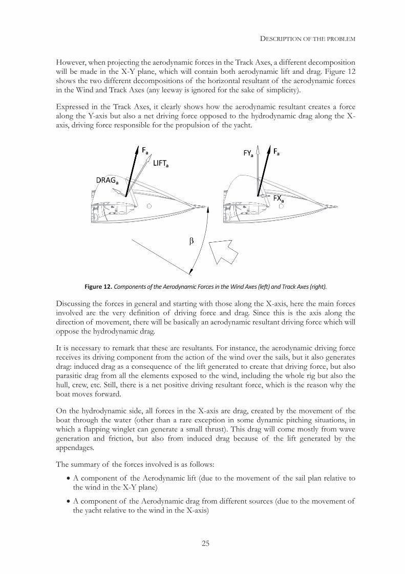
DESCRIPTION OF THE PROBLEM
25
However, when projecting the aerodynamic forces in the Track Axes, a different decomposition will be made in the X-Y plane, which will contain both aerodynamic lift and drag. Figure 12 shows the two different decompositions of the horizontal resultant of the aerodynamic forces in the Wind and Track Axes (any leeway is ignored for the sake of simplicity).
Expressed in the Track Axes, it clearly shows how the aerodynamic resultant creates a force along the Y-axis but also a net driving force opposed to the hydrodynamic drag along the X-axis, driving force responsible for the propulsion of the yacht.
Discussing the forces in general and starting with those along the X-axis, here the main forces involved are the very definition of driving force and drag. Since this is the axis along the direction of movement, there will be basically an aerodynamic resultant driving force which will oppose the hydrodynamic drag.
It is necessary to remark that these are resultants. For instance, the aerodynamic driving force receives its driving component from the action of the wind over the sails, but it also generates drag: induced drag as a consequence of the lift generated to create that driving force, but also parasitic drag from all the elements exposed to the wind, including the whole rig but also the hull, crew, etc. Still, there is a net positive driving resultant force, which is the reason why the boat moves forward.
On the hydrodynamic side, all forces in the X-axis are drag, created by the movement of the boat through the water (other than a rare exception in some dynamic pitching situations, in which a flapping winglet can generate a small thrust). This drag will come mostly from wave generation and friction, but also from induced drag because of the lift generated by the appendages.
The summary of the forces involved is as follows:
A component of the Aerodynamic lift (due to the movement of the sail plan relative to the wind in the X-Y plane)
A component of the Aerodynamic drag from different sources (due to the movement of the yacht relative to the wind in the X-axis)
Figure 12. Components of the Aerodynamic Forces in the Wind Axes (left) and Track Axes (right).
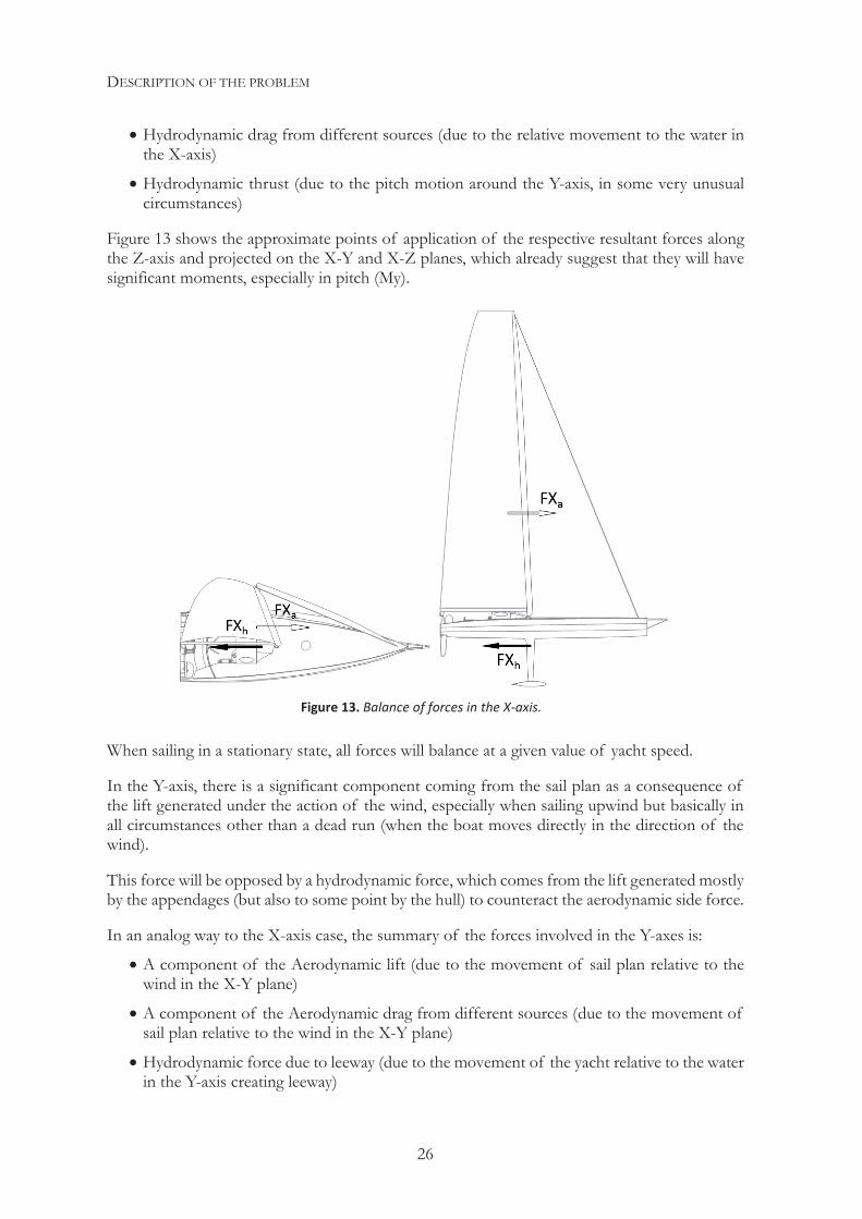
DESCRIPTION OF THE PROBLEM
26
Hydrodynamic drag from different sources (due to the relative movement to the water in the X-axis)
Hydrodynamic thrust (due to the pitch motion around the Y-axis, in some very unusual circumstances)
Figure 13 shows the approximate points of application of the respective resultant forces along the Z-axis and projected on the X-Y and X-Z planes, which already suggest that they will have significant moments, especially in pitch (My).
When sailing in a stationary state, all forces will balance at a given value of yacht speed.
In the Y-axis, there is a significant component coming from the sail plan as a consequence of the lift generated under the action of the wind, especially when sailing upwind but basically in all circumstances other than a dead run (when the boat moves directly in the direction of the wind).
This force will be opposed by a hydrodynamic force, which comes from the lift generated mostly by the appendages (but also to some point by the hull) to counteract the aerodynamic side force.
In an analog way to the X-axis case, the summary of the forces involved in the Y-axes is:
A component of the Aerodynamic lift (due to the movement of sail plan relative to the wind in the X-Y plane)
A component of the Aerodynamic drag from different sources (due to the movement of sail plan relative to the wind in the X-Y plane)
Hydrodynamic force due to leeway (due to the movement of the yacht relative to the water in the Y-axis creating leeway)
Figure 13. Balance of forces in the X-axis.
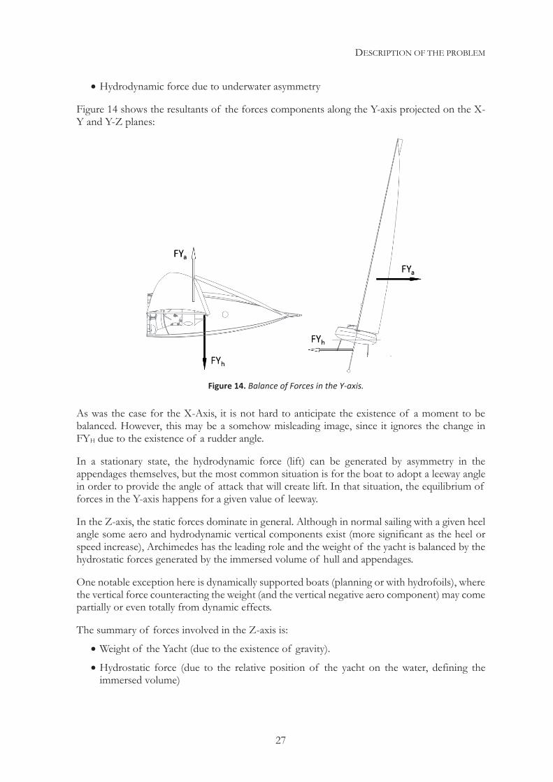
DESCRIPTION OF THE PROBLEM
27
Hydrodynamic force due to underwater asymmetry
Figure 14 shows the resultants of the forces components along the Y-axis projected on the X-Y and Y-Z planes:
As was the case for the X-Axis, it is not hard to anticipate the existence of a moment to be balanced. However, this may be a somehow misleading image, since it ignores the change in FYH due to the existence of a rudder angle.
In a stationary state, the hydrodynamic force (lift) can be generated by asymmetry in the appendages themselves, but the most common situation is for the boat to adopt a leeway angle in order to provide the angle of attack that will create lift. In that situation, the equilibrium of forces in the Y-axis happens for a given value of leeway.
In the Z-axis, the static forces dominate in general. Although in normal sailing with a given heel angle some aero and hydrodynamic vertical components exist (more significant as the heel or speed increase), Archimedes has the leading role and the weight of the yacht is balanced by the hydrostatic forces generated by the immersed volume of hull and appendages.
One notable exception here is dynamically supported boats (planning or with hydrofoils), where the vertical force counteracting the weight (and the vertical negative aero component) may come partially or even totally from dynamic effects.
The summary of forces involved in the Z-axis is:
Weight of the Yacht (due to the existence of gravity).
Hydrostatic force (due to the relative position of the yacht on the water, defining the immersed volume)
Figure 14. Balance of Forces in the Y-axis.
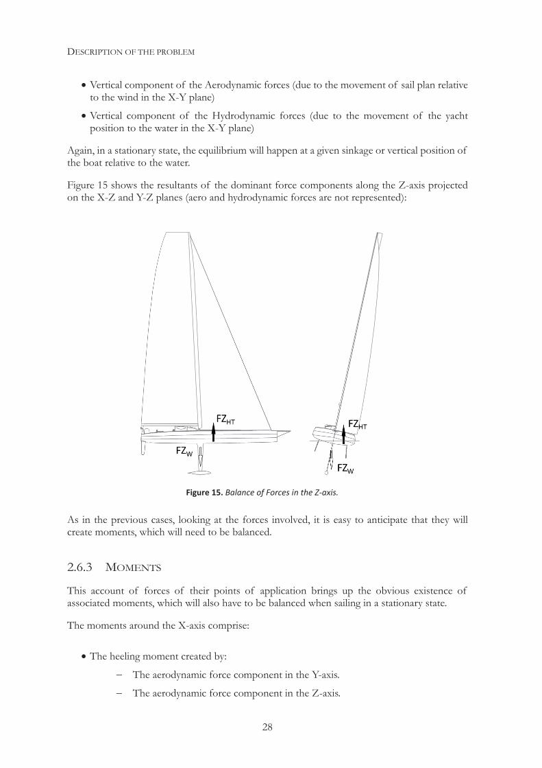
DESCRIPTION OF THE PROBLEM
28
Vertical component of the Aerodynamic forces (due to the movement of sail plan relative to the wind in the X-Y plane)
Vertical component of the Hydrodynamic forces (due to the movement of the yacht position to the water in the X-Y plane)
Again, in a stationary state, the equilibrium will happen at a given sinkage or vertical position of the boat relative to the water.
Figure 15 shows the resultants of the dominant force components along the Z-axis projected on the X-Z and Y-Z planes (aero and hydrodynamic forces are not represented):
As in the previous cases, looking at the forces involved, it is easy to anticipate that they will create moments, which will need to be balanced.
2.6.3 MOMENTS
This account of forces of their points of application brings up the obvious existence of associated moments, which will also have to be balanced when sailing in a stationary state.
The moments around the X-axis comprise:
The heeling moment created by:
The aerodynamic force component in the Y-axis.
The aerodynamic force component in the Z-axis.
Figure 15. Balance of Forces in the Z-axis.
DESCRIPTION OF THE PROBLEM
29
The lift generated by the hydrodynamic forces.
The roll moment (which could have either sign) created by the vertical component generated by the hydrodynamic forces.
The moment from the asymmetrical distribution of weight due to the asymmetry generated by heel or movements of weights (like the placing of crew or asymmetric ballast to increase the stability)
The moment from hydrostatic forces, due to the immersed volume.
All these moments will find an equilibrium point defined by a given heel angle.
Around the Y-Axis, the moments will comprise:
The pitch moment created by:
The aerodynamic driving force.
The aerodynamic force component in the Z-axis.
The vertical component generated by the hydrodynamic forces.
The hydrodynamic drag.
The moment from the longitudinal position of the yacht weight or movements of weight (like longitudinal placement of crew or ballast to correct pitch)
The moment from hydrostatic forces due to the immersed volume.
All these moments will find an equilibrium point defined by a given trim angle.
Finally, around the Z-Axis the moments will be generated by:
The aerodynamic force component in the Y-axis.
The aerodynamic force component in the X-axis.
The hydrodynamic lift (especially from the steering elements, like rudders, given their large moment arm).
The hydrodynamic drag.
All these moments will find an equilibrium point defined by a given setting of a “steering parameter”, which in most cases will be a rudder angle, responsible both for steering and for maintaining a straight course, keeping the sum of moments equal to zero.
It is necessary to point out that moments do not only originate from the combination of resultants from different origins. One single cause (such as an incoming flow) can generate a number of forces in the same axis which may in some cases nearly cancel each other’s into a small resultant but still have a significant resulting moment.
A good example of this is the yaw moment present in the case when a boat with an improper yaw balance sails with its keel generating positive lift force (in the Y axes), but requires the rudder to generate negative lift force to maintain a stable course.
Regarding the moments around the X-axis, it must be pointed out that the lever arm between the aerodynamic driving force and the hydrodynamic drag increases with heel angle, as the left image in Figure 13 shows. This is the reason why weather helm (a positive rudder angle, required
DESCRIPTION OF THE PROBLEM
30
to generate more yaw moment in order to maintain a straight course) increases with heel. Simply considering the relative longitudinal positions of the aerodynamic and hydrodynamic centers of effort (as shown in the left image of Figure 14) is not sufficient to define the yaw equilibrium.
2.6.4 MOMENTS AND FORCES CREATED BY NON-STATIONARY MOTIONS
Up until now, only the forces and moments generated when the boat is sailing in a stationary state have been discussed (where the movement is constrained to the X-Y plane and no accelerations other than the gravity are involved). When discussing the full dynamics of the sailing yacht, new sources of forces and moments appear due to the additional motions, as well as inertial forces because of the accelerations.
At this point, they will be briefly introduced, and their origins discussed, without making an exhaustive description:
Pitch motions will alter the flow over the hull and appendages, but more significantly the flow over the sail plan. They will induce an additional flow velocity component that will need to be taken into account when calculating the apparent wind angle and speed, as it will alter the geometry of the wind triangle.
Yaw motions will also have an effect on the sail plan, but this time their influence on the appendages may be more important, and especially on the rudder, as its angle of attack will be affected by the side component generated by the yaw rotation around a point situated forward.
Roll motions will introduce a side component on both the sail plan and appendages, thus changing the angle of attack and the speed of their respective incoming flows.
Vertical motions will normally only be significant when a hydrodynamic vertical force is present, as is the case with hydrofoils, and they will alter the angle and speed of the incoming flow by adding a vertical component.
Finally, any acceleration will create forces and moments due to the masses and moments of inertia of the yacht, but also due to the added mass of water to be considered in some cases, adding an additional layer of complexity to the problem.
It is necessary to note that at this point we are referring to the effects of the motions and accelerations themselves, not the changes of position that they generate. The changes in position will affect the forces and moments involved, but these will be analyzed from a strictly static point of view, and even in a time-domain analysis they will be considered as a succession of static situations.
Also, any motions other than those in the X-Y plane will have an oscillatory nature, as continuous translation or rotation in those axis would necessarily lead to losing the desired course in the best case (continuous rotation around the Z-axis), or capsizing in all other cases.
THE ORIGIN OF FORCES.
31
3| THE ORIGIN OF FORCES Having reached this point, it is easy to understand that one of the keys to model the physic phenomena involved in the equilibrium of a yacht while sailing is an adequate understanding of the origin of the forces to which the yacht is subject. This will be necessary in order to properly study the balance of forces when sailing in a stationary state, or to simply account for their effects in a non-stationary situation.
The knowledge about the forces must happen in two different levels:
In a first level, it is necessary to properly identify the origin of the forces themselves, their nature and the physical phenomena causing them.
The second level, also linked to their origin, is about qualitatively identifying what those forces depend on, and quantitatively how important that dependency is.
These two levels really depend on each other and, as A. Claughton describes in “Sailing Yacht Design” (7) in a clever and elegant way, “Sailing Yachts are uniquely complex vehicles, which operate in the interface between two fluids, deriving propulsion from one and support from the other, both subject to environmental effects. It is not surprising that many aspects of Yacht Design resist perfect mathematical analysis”. Performance assessment is clearly one of those aspects.
Therefore, this Chapter will be dedicated to reviewing the origin of those forces and their main dependencies, in order to then try to quantify them to the point of expressing the forces as functions of the variables or parameters they depend on.
Amongst these parameters are the environmental conditions (which will also affect the incoming flows), but also the description of the geometries involved, trying to identify the elements which are relevant to the calculations, in other words, which are significant design parameters with an impact on forces.
With all that information, it will be possible to perform calculations for a given design, or to estimate the effect that some changes in that design would have on the generated forces, and thus performance.
Also, in some cases it will be the absolute value of the calculated forces that will be relevant, but in some others it will be the relative effect of some parametric changes on those forces. These two situations are not mutually exclusive but may require a different level of accuracy.
As a summary of specific steps, the purpose of this Chapter is to describe the origin of the forces, to provide guidelines and cautions in their calculation, to refer to the known available analytical models to evaluate them and to propose strategies to build these models for use in a VPP.
HOW ARE FORCES GENERATED In the previous Chapter, it was already outlined how the main forces involved are created. At this point, the idea is to make a detailed list of possible forces with consideration of their origin,
THE ORIGIN OF FORCES
32
significance, and importance in the global equilibrium. In addition, there will be a brief discussion about which of those forces have adjustments that can be changed while sailing, or, in their virtual equivalent, parameters that can be optimized in the process of performing a VPP calculation.
3.1.1 STATIC FORCES
Static forces play an important role in the equilibrium of any boat as they define how it floats on the water. This is the most basic requirement for equilibrium for any floating artefact.
The two main static forces are a consequence of the boat’s mass and of the volume of water it displaces. When floating at rest, the Archimedes’ Principle balances the boat’s weight with the displacement (weight of displaced volume of water).
Weight will be characterized by the mass and center of gravity (CG), and displacement will be characterized by the displaced volume and by the density of the fluid in which the boat is floating, and by the center of that volume or center of buoyancy (CB). For an equilibrium at rest, the X and Y coordinates of those centers must be the same. The X coordinate will condition at what trim angle of the boat the static equilibrium happens (conditioned by the longitudinal stability), and the Y coordinate, at what heel angle the static equilibrium happens (conditioned by the transverse stability).
Without getting into an explanation of hydrostatics, let us just say that when the boat changes its heel or trim, the center of the volume will move until its X and Y coordinates match those of the center of gravity of the mass, which will change as well with movement. As long as this match is possible, the boat will be stable. Beyond that point, the boat will capsize.
The Z coordinate of the center of gravity of the mass (VCG), along with the changes in the geometry of the immersed volume, will determine when stability will vanish.
However, there are other weights to consider in addition to the weight of the boat.
On one hand, it is possible to have a moving weight, like crew or ballast, which is always present on board, and as such it is included in the total yacht weight. The movable weight will need to have its mass and range of movement or permitted positions defined. This movement can be pre-determined, or be described as a variable, subject to optimization due to its effect on stability and sailing trim of the yacht.
It is also possible to consider the presence of water ballast that can be added or removed. In this case, its addition will have to be taken into consideration towards the calculation of the total weight as it forces a change in the displacement. As it happened in the previous case, it will have a range of movement or possible positions (sometimes defined by which tanks are available to fill).
Two other factors will have an influence in the static forces, both derived from the movable appendages, but with a different nature.
The first one is the case of retractable boards (centerboards, daggerboards, retractable foils, etc.), where an appendage can be totally or partially immersed, changing the characteristics of its immersed volume as well as the position of the center of gravity of the mass of the moved element. These boards could also be oriented in one or more axis.

THE ORIGIN OF FORCES.
33
The second one has the best example in canting keels, in which a ballasted torpedo is moved to windward in order to increase the righting moment induced by its weight. In this case, there is a change in both the center of the immersed volume and its center of gravity, but the immersed volume remains constant.
In these two cases, the range of possible movements needs to be defined.
However, special caution must be taken regarding the movement of these elements and the position of the boat, to guarantee that the immersed volume is always accurately evaluated. This avoids, for instance, situations in which an immersed board coming out of the water due to heel goes unnoticed and thus, it is not properly evaluated.
As a summary for the static forces, all that is required is a knowledge of the global weight and its center of gravity, and a calculated value and position of the centroid of the total immersed volume (which will normally be a sum of the immersed part of the hull and appendages).
These forces are the dominant ones in the Z-axis of the Track Axes, and given their nature, they have no components in other axes. The only exception happens when significant dynamic vertical forces are present, as is the case in planing hulls or foil assisted boats.
While these static forces are not affected by the movement itself, they are indirectly influenced by it, given that they depend on the boat’s position (that will change because of the movement). For instance, the aerodynamic driving force creates a bow down pitch moment that will induce a pitch motion. This will have the effect of changing the position of the global center of gravity, but even more so the longitudinal center of the immersed volume.
The effect of the free surface with partially filled tanks must also be taken into consideration when there are changes in heel or trim, to calculate the CG of its content towards the global CG calculation.
Another “modifier” of the static forces, often ignored but which can sometimes be significant, is the loss of stability due to the change in the water surface shape from its ideal flat condition at rest. This can be accentuated by ocean waves, but it happens also as the hull moves through calm water. This effect becomes more significant in the high range of Froude numbers, sailing in displacement mode, when a wave trough appears close to the maximum beam of the boat (where the changes in immersed volume have the largest effects on the transverse stability of the boat).
This phenomenon is caused by the movement of the boat, but it has a hydrostatic nature through the change in the shape of the immersed volume and of its center, resulting in a loss in stability. It is especially important in boats with high LWL/BWL and /LWL1/3 ratios and low CM. A number of corrections are available, which take into account these parameters and the Froude number.
This effect should not be confused with the changes in stability due to the asymmetrical pressure forces created by the flow of the water moving around the hull and/or appendages, with a clearly hydrodynamic origin.
Normally these forces are calculated originally in “virtual” Track Axes (given that there “is” no movement). Leeway has to be taken into consideration when translating these forces into the actual Track Axes in the normal situation with the boat in motion.
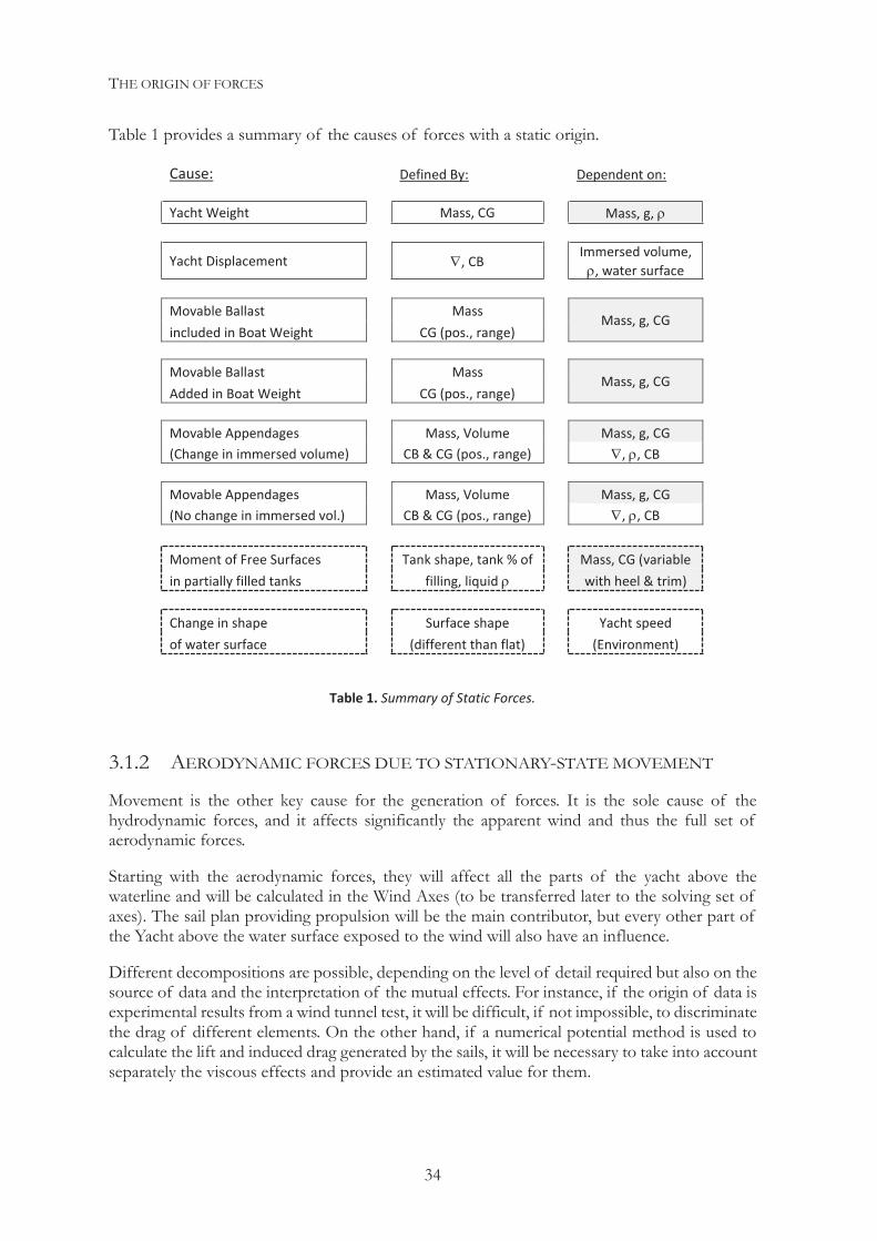
THE ORIGIN OF FORCES
34
Table 1 provides a summary of the causes of forces with a static origin.
3.1.2 AERODYNAMIC FORCES DUE TO STATIONARY-STATE MOVEMENT
Movement is the other key cause for the generation of forces. It is the sole cause of the hydrodynamic forces, and it affects significantly the apparent wind and thus the full set of aerodynamic forces.
Starting with the aerodynamic forces, they will affect all the parts of the yacht above the waterline and will be calculated in the Wind Axes (to be transferred later to the solving set of axes). The sail plan providing propulsion will be the main contributor, but every other part of the Yacht above the water surface exposed to the wind will also have an influence.
Different decompositions are possible, depending on the level of detail required but also on the source of data and the interpretation of the mutual effects. For instance, if the origin of data is experimental results from a wind tunnel test, it will be difficult, if not impossible, to discriminate the drag of different elements. On the other hand, if a numerical potential method is used to calculate the lift and induced drag generated by the sails, it will be necessary to take into account separately the viscous effects and provide an estimated value for them.
Cause: Defined By: Dependent on: Yacht Weight Mass, CG Mass, g,
Yacht Displacement , CB Immersed volume,
, water surface
Movable Ballast Mass Mass, g, CG included in Boat Weight CG (pos., range) Movable Ballast Mass Mass, g, CG Added in Boat Weight CG (pos., range) Movable Appendages Mass, Volume Mass, g, CG (Change in immersed volume) CB & CG (pos., range) , , CB
Movable Appendages Mass, Volume Mass, g, CG (No change in immersed vol.) CB & CG (pos., range) , , CB
Moment of Free Surfaces Tank shape, tank % of Mass, CG (variable in partially filled tanks filling, liquid with heel & trim) Change in shape Surface shape Yacht speed of water surface (different than flat) (Environment)
Table 1. Summary of Static Forces.
THE ORIGIN OF FORCES.
35
This suggests that the best decomposition depends strongly on the source of data. At this point, we will consider a scheme both based on physical phenomena and related to analytical models, and we will try to make a reasonable separation between these, to help understand the actual source of the forces. Later, it will be shown how that separation will be of great importance even when the source of data gives a full accurate global force, like the ideal result of a wind tunnel test.
Another important point to consider regarding the origin of forces is that, using the aerodynamic forces as example, each element, in this case sail, affects the flow and forces on the other elements (other sails) in a more or less significant way.
In some cases, this interaction can be determinant. For instance, in a sail plan composed by a mainsail and a headsail sailing upwind, two important effects will happen: the presence of the mainsail will create a downwash in the headsail, which will increase its apparent wind angle and driving force, while the headsail will create an upwash effect on the mainsail with opposite consequences. This makes combining the forces from the two sails a far from trivial task when calculated analytically.
Similar interaction happens with hydrodynamic forces, and there is no single answer regarding how to deal with it other than a scientifically educated “common sense”.
At this point, when defining the origin of forces, we will try to look at them individually and identify the cross effects, as it would be done when trying to build up a total resultant based on strictly analytical deductions. When discussing parametric models specifically, different alternatives will be shown and/or proposed.
Going back to the starting point with the aerodynamic forces, the main obvious forces are those generated by the propulsion system, in which the lift generated by the sail plan, at this point defined as sails and mast, is perpendicular to the incoming wind vector. Because of the three dimensional effects, this will generate an induced drag (by definition, in the direction of the wind vector) which will depend on the generated lift but also on the effective span of the sail plan.
Two additional sources of drag will come from the sail plan. One will be a viscous component, which may include separation effects or not, dependent on the wind speed and geometry. Another will be also a viscous drag component, usually called parasitic quadratic drag, but this time dependent on the squared lift coefficient.
The resultant of all these forces will be applied at the center of effort of the sail plan (by definition), which will be approximately at its center of area. A more detailed estimate considering wind gradient, the area and lift distribution, and the effective span, would provide the determination of the center of effort.
Also, different depowering schemes will have an effect on the lift and drag components, which can be quantified.
The sail plan is being discussed as a single item, but each sail and the mast itself will generate their own forces as pointed out before. These forces could be combined into a global resultant in different ways.
For those components of the boat which are not intended to generate a driving force, the viscous drag they generate will be referred to as “parasitic” drag, or in general, as “windage”.
THE ORIGIN OF FORCES
36
This is, for instance, the case for the rig (mainly constituted by wires exposed to the incoming airflow), but also for all the other elements of the yacht above the water.
Some boats may have a clean hull and deck for which a low drag coefficient can be estimated and exposed area measured. Some others have deckhouses with a large area and bigger drag coefficients due to flow separation. There are in the literature different sources of information to estimate these drag coefficients with reasonably accuracy, like the classic “Fluid-Dynamic Drag” from S.F. Hoerner (13) (still a valid source for this type of information).
Depending on the proximity of the sails to the deck (especially, when the gap between them is small) some end plate effects can be expected. They may be significant in the case of multihulls in which a careful aerodynamic design of the cross structure between hulls, also called “platform”, can favor significantly the efficiency of the sail plan and even generate non insignificant vertical forces, affecting displacement but also stability. This is one of the situations in which significant cross effects between different elements are not negligible.
Virtually any element exposed to the wind will create some lift (in most cases insignificant compared to that of the sail plan) and certainly drag.
In addition, the height above the water of any of those elements will define the wind speed to which they are subject because of the wind gradient (and therefore the local incoming flow angle). This should be calculated and taken into account. The effects of wind gradient become obvious, for instance, when thinking about the difference in height and wind speed that can be expected in the top of the mast compared to the deck, also with the already discussed effects on the apparent wind angle calculations.
Height will also be affected by heel, especially when considering the sail plan and the rig. On the other hand, the trim angle is usually so small that the cosine of its value makes its effect on height negligible.
The importance of understanding the mechanisms by which the forces are generated must be reiterated, in order to be able to judge what should be calculated and how, and how accurate that calculation should be. Multihulls are an excellent example of this for two reasons: their usually high speeds create high apparent wind speeds and therefore the forces from aerodynamic origin become a more significant fraction of the total drag, but also the complex cross structure of the hulls and the fact that the windward hull is airborne allows room for design optimization.
These configurations really show the need to be able to judge which elements should be considered, evaluated and analyzed regarding the generation of lift/drag. That may require choosing an appropriate method capable of capturing these effects (prior to having a full knowledge of the involved phenomena), rather than making a rough estimate of parasitic drag only based on an exposed area and an “off the shelf ” drag coefficient.
Different parameters can be optimized from the design point of view. Even for a given design, there is a set of optimization variables included in the concept of “sail trim”, which is related to the actual adjustments of the sail while sailing. This is the original depowering scheme present since Kerwin’s VPP (as a simple reefing factor there) and which has evolved to a more precise depowering scheme with its best analytical example in the most recent IMS VPP.
However, new options have also appeared related to sail trim and more complex and realistic trimming parameters. Those are not only related to depowering, but try to reproduce the actual controls that sailors use to adjust the sail depth and twist, along with the sheeting angle. A more
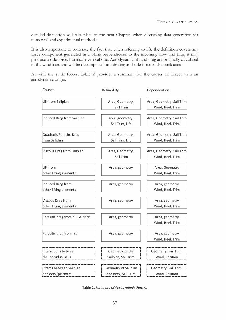
THE ORIGIN OF FORCES.
37
detailed discussion will take place in the next Chapter, when discussing data generation via numerical and experimental methods.
It is also important to re-iterate the fact that when referring to lift, the definition covers any force component generated in a plane perpendicular to the incoming flow and thus, it may produce a side force, but also a vertical one. Aerodynamic lift and drag are originally calculated in the wind axes and will be decomposed into driving and side force in the track axes.
As with the static forces, Table 2 provides a summary for the causes of forces with an aerodynamic origin.
Cause: Defined By: Dependent on: Lift from Sailplan Area, Geometry, Area, Geometry, Sail Trim Sail Trim Wind, Heel, Trim
Induced Drag from Sailplan Area, geometry, Area, Geometry, Sail Trim Sail Trim, Lift Wind, Heel, Trim
Quadratic Parasite Drag Area, Geometry, Area, Geometry, Sail Trim from Sailplan Sail Trim, Lift Wind, Heel, Trim
Viscous Drag from Sailplan Area, Geometry, Area, Geometry, Sail Trim Sail Trim Wind, Heel, Trim
Lift from Area, geometry Area, Geometry other lifting elements Wind, Heel, Trim
Induced Drag from Area, geometry Area, geometry other lifting elements Wind, Heel, Trim
Viscous Drag from Area, geometry Area, geometry other lifting elements Wind, Heel, Trim
Parasitic drag from hull & deck Area, geometry Area, geometry Wind, Heel, Trim
Parasitic drag from rig Area, geometry Area, geometry Wind, Heel, Trim
Interactions between Geometry of the Geometry, Sail Trim, the individual sails Sailplan, Sail Trim Wind, Position
Effects between Sailplan Geometry of Sailplan Geometry, Sail Trim, and deck/platform and deck, Sail Trim Wind, Position
Table 2. Summary of Aerodynamic Forces.
THE ORIGIN OF FORCES
38
3.1.3 HYDRODYNAMIC FORCES DUE TO STATIONARY MOVEMENT
When discussing hydrodynamics, the calculation domain is limited to the immersed part of the boat (with the exception of spray drag), but with consideration to the effects on the water surface. Given the difference between the densities of water and air, the effects of the air on the water surface are ignored, other than as an environmental factor, which can create waves. Those, if present, will be considered both by themselves and in relation to the resistance added in waves.
When considering modern boats, the appendages which act as lifting surfaces are clearly separated from the hull so it is easier to make a distinction between them, and between the ways they operate. That was not the case in more traditional hulls with a long integrated keel, which would extend all the way from the bow to the stern. That and any other possible intermediate step in design evolution could be considered, making the problem more complicated.
The main discussion here will be related to modern yachts, when discussing the origin of forces. It is important to remember that some of the distinctions that will be made have sometimes less clear boundaries, and once again, there are complex interactions between different parts, which sometimes are even difficult to differentiate. Limiting this analysis to a standard modern yacht, in which there is a hull with distinctive appendages attached to it, the following sources of forces can be identified.
The hull, responsible for most of the displacement, will have as one of the main force contributors, due to its movement through the water, the residuary drag, a component of potential origin which is responsible for the formation of waves in the free surface (therefore causing this source of drag). This is called wave drag. But since it is traditionally calculated as being all sources of drag minus the viscous terms, it is also called residuary drag.
The other significant source of drag from the hull is the friction drag, with a viscous origin, and which increases with the squared speed. The residuary drag however, has a variable increase with speed, which makes it small for low speeds and the dominant component when sailing at high speeds in displacement mode.
A third small contributor will be a potential drag but of viscous origin. Due to the existence of the viscosity, a boundary layer develops with a given thickness, altering the field of fluid velocities and thus pressures. While not irrelevant, it certainly is a much smaller component in sailing yachts than in large ships. In the case of large ships, their long length contributes to a thick boundary layer in the stern area of the hull.
Heel and trim have an influence on the hull drag. These sources of “added drag” can be described as drag components by themselves. However, it is preferable to take them into consideration either when calculating the actual hull position or as a modifier of the forces generated with a baseline heel and trim in a reference flotation. In the latter case, the changes in drag are normally referred to as heel or trim drag.
The hull moving through the water will also generate some vertical forces, even for full bodied displacement boats, with some drag associated, which can be considered included in the residuary drag (consistent with its definition). With planing boats, the generation of the extra vertical force will have an effect on drag, but combined with a reduction in displacement. This would be considered part of the so-called residuary drag, and although it also creates waves, these are generated by a different mechanism than those created when in displacement mode.
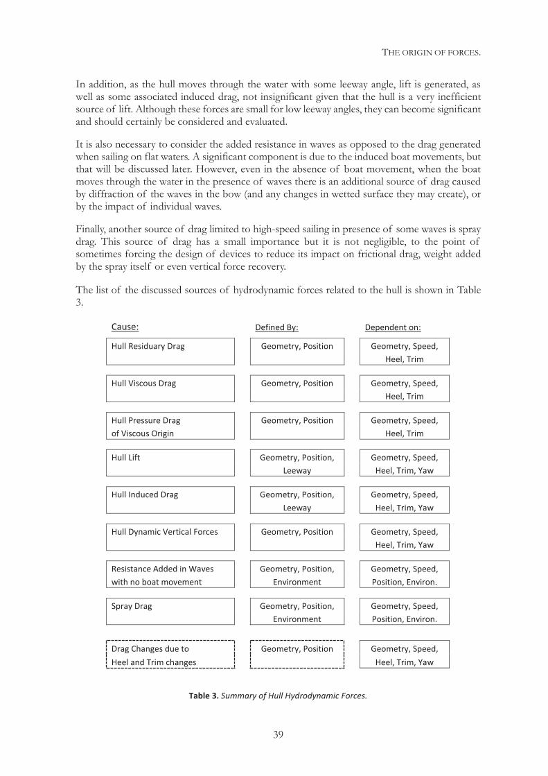
THE ORIGIN OF FORCES.
39
In addition, as the hull moves through the water with some leeway angle, lift is generated, as well as some associated induced drag, not insignificant given that the hull is a very inefficient source of lift. Although these forces are small for low leeway angles, they can become significant and should certainly be considered and evaluated.
It is also necessary to consider the added resistance in waves as opposed to the drag generated when sailing on flat waters. A significant component is due to the induced boat movements, but that will be discussed later. However, even in the absence of boat movement, when the boat moves through the water in the presence of waves there is an additional source of drag caused by diffraction of the waves in the bow (and any changes in wetted surface they may create), or by the impact of individual waves.
Finally, another source of drag limited to high-speed sailing in presence of some waves is spray drag. This source of drag has a small importance but it is not negligible, to the point of sometimes forcing the design of devices to reduce its impact on frictional drag, weight added by the spray itself or even vertical force recovery.
The list of the discussed sources of hydrodynamic forces related to the hull is shown in Table 3.
Cause: Defined By: Dependent on:
Hull Residuary Drag Geometry, Position Geometry, Speed, Heel, Trim
Hull Viscous Drag Geometry, Position Geometry, Speed, Heel, Trim
Hull Pressure Drag Geometry, Position Geometry, Speed, of Viscous Origin Heel, Trim
Hull Lift Geometry, Position, Geometry, Speed, Leeway Heel, Trim, Yaw
Hull Induced Drag Geometry, Position, Geometry, Speed, Leeway Heel, Trim, Yaw
Hull Dynamic Vertical Forces Geometry, Position Geometry, Speed, Heel, Trim, Yaw
Resistance Added in Waves Geometry, Position, Geometry, Speed, with no boat movement Environment Position, Environ.
Spray Drag Geometry, Position, Geometry, Speed, Environment Position, Environ.
Drag Changes due to Geometry, Position Geometry, Speed, Heel and Trim changes Heel, Trim, Yaw
Table 3. Summary of Hull Hydrodynamic Forces.

THE ORIGIN OF FORCES
40
The next significant group of forces comes from the appendages, which perform fundamentally as lifting surfaces to compensate the side force component generated by the sailplan.
The lift generated by the appendages will depend on the asymmetry of the flow on them, created either by altering their shape (rotation, addition of flaps or simply asymmetrical design) or via the creation of an angle of attack (leeway).
This lift will have a corresponding cost in induced drag, depending on the amount of lift generated and the effective span of the appendages.
The appendages will also generate frictional drag because of viscosity, as well as the usual component of potential drag due to the existence of viscosity, very small in this case since the significant length is small and so is the boundary layer thickness. Instead, a parasitic quadratic drag, dependent of the squared lift, will exist as in the aerodynamic case.
Another source of drag is in the junction of the appendages to the hull, named interference drag due to its cause in the interference between the boundary layers of the hull and the appendages at the attachment point.
These are the main sources of drag, but there are also other possible sources of parasitic drag in the case of other elements attached to hull or appendages, like propellers, shafts, anodes, speed transducers, openings and basically anything which does not have as the main purpose the generation of lift or displacement, creating as little drag as possible.
We have considered the appendages functioning individually, given that their positions are normally distant relative to their size, as opposed to a sail plan. It is then possible to build a full model from the individual forces, but some corrections may be necessary given that some degree of interaction exists in most cases.
The interaction can be small with little more effect than, for instance, the rudder being exposed to a lower fluid velocity because of being partially in the wake of the keel or having a bigger fraction of its span inside the boundary layer of the hull. Nevertheless, the effect can be more significant, especially with lift generation, when more complex interactions may happen due to the vortices shedding from the keel, in a phenomenon that normally shows a strong dependency with leeway.
The degree of interference can, to some point, be anticipated and evaluated when deciding how to calculate the forces. It can have a significant importance, especially in the case of keels with designs which depart from a traditional vertical fin (with bulbs, winglets etc.).
Regarding appendages, we have referred so far to the lift generated to counteract the side force from the sail plan, but there is a case where they can generate a very important vertical force, for example, when hydrofoils are present. These can be independent devices intended to generate lift, with its main component being a vertical force, or they can be appendages designed to generate both a side force and a vertical force.
Table 4 intends to provide a collected list of the sources of hydrodynamic drag coming from the appendages.
As the table shows, there is another type of “wave generating” drag, and that is the one derived from surface piercing appendages (or even appendages in close proximity to the free surface). This is the case of fully hydrofoil-supported boats, or even many more conventional designs
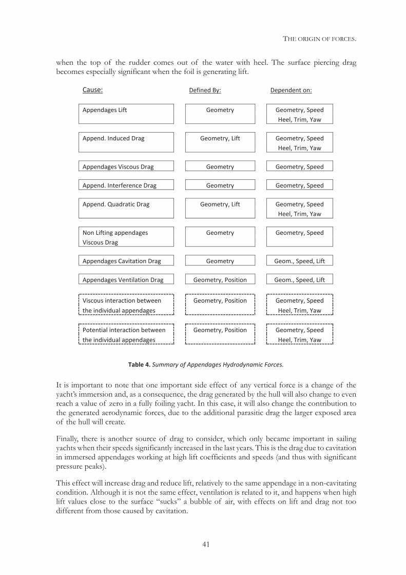
THE ORIGIN OF FORCES.
41
when the top of the rudder comes out of the water with heel. The surface piercing drag becomes especially significant when the foil is generating lift.
It is important to note that one important side effect of any vertical force is a change of the yacht’s immersion and, as a consequence, the drag generated by the hull will also change to even reach a value of zero in a fully foiling yacht. In this case, it will also change the contribution to the generated aerodynamic forces, due to the additional parasitic drag the larger exposed area of the hull will create.
Finally, there is another source of drag to consider, which only became important in sailing yachts when their speeds significantly increased in the last years. This is the drag due to cavitation in immersed appendages working at high lift coefficients and speeds (and thus with significant pressure peaks).
This effect will increase drag and reduce lift, relatively to the same appendage in a non-cavitating condition. Although it is not the same effect, ventilation is related to it, and happens when high lift values close to the surface “sucks” a bubble of air, with effects on lift and drag not too different from those caused by cavitation.
Cause: Defined By: Dependent on: Appendages Lift Geometry Geometry, Speed Heel, Trim, Yaw
Append. Induced Drag Geometry, Lift Geometry, Speed Heel, Trim, Yaw
Appendages Viscous Drag Geometry Geometry, Speed
Append. Interference Drag Geometry Geometry, Speed
Append. Quadratic Drag Geometry, Lift Geometry, Speed Heel, Trim, Yaw
Non Lifting appendages Geometry Geometry, Speed Viscous Drag
Appendages Cavitation Drag Geometry Geom., Speed, Lift
Appendages Ventilation Drag Geometry, Position Geom., Speed, Lift
Viscous interaction between Geometry, Position Geometry, Speed the individual appendages Heel, Trim, Yaw
Potential interaction between Geometry, Position Geometry, Speed the individual appendages Heel, Trim, Yaw
Table 4. Summary of Appendages Hydrodynamic Forces.
THE ORIGIN OF FORCES
42
3.1.4 FORCES DUE TO NON-STATIONARY MOTIONS
This is a group of forces which would not be considered when facing the stationary problem in flat water, but that requires special attention when something creates non-stationary motions in the boat.
The first potential cause of motions is the exposition of the boat to the waves, which will generate forces and motions. These will be amplified when the boat is moving through those waves.
The second possible cause of motions is an imbalance of the forces, which are in equilibrium when sailing at a stationary state. This imbalance can appear from a change in trim, from weight movement or simply from a change in the wind conditions.
Either way, as per the second of Newton’s laws, accelerations will be generated, which will have an effect on the boat’s performance. It is also necessary to keep in mind that if in a conventional powerboat propulsion is affected by the motions, in a sailing yacht the effects are dramatic. Even in the simplest case of a boat sailing in regular waves, there will be a serious impact on the driving force.
With this in mind, the next task will be to identify how forces will be generated by the boat’s motions, whether caused by the induced velocities and accelerations or as a consequence of the changes in position.
Thinking in Boat Axes and starting with translations, surge movements changing the stationary-state speed will on one hand create a change in drag, and as a consequence, a differential force accelerating or slowing down the boat. This change in speed will also change the lift generated by the appendages but even more so the forces on the sail plan, given that not only the apparent wind speed will change but also the angle.
These changes in speed in the X-Axis may happen because of a change in the wind conditions (speed or angle), sail trim (adjustments), boat position, or even an impact with a wave.
Sway movements will mostly have an impact on the lift generated by appendages, since they change the angle of the incoming flow, and to a lesser extent the speed. A similar situation happens with the sailplan, affecting the apparent wind speed and angle.
Changes in speed in the Y-Axis may happen because of a change in the wind conditions, sail trim (speed or angle), change of the immersion in a board or angle of rudders or keel tabs. The side impact of a wave would also generate sway.
Heave movements are less common in displacement boats, but very common in foil-assisted yachts as they change the angle of attack of the hydrofoils, therefore affecting the vertical force they generate.
Several reasons can cause changes in the speed in the Z-Axis, ranging from a previous change of the foil position to a simple change in the yacht speed that will alter the vertical force proportional to its squared value.
At this point, it is important to make a clarification. There are coupled effects between degrees of freedom. For instance, a heave movement will also affect the immersed area of the boards
THE ORIGIN OF FORCES.
43
in a foiling yacht, and that will have the consequence of generating a sway movement, given the imbalance in the Y-Axis forces which will most likely happen.
This is just a simple example, but interactions are abundant and complex. However, a more detailed analysis of the previous example shows that the coupling we have pointed out depends on the position, which changes because of the movement, but it is the position rather than the movement itself that will change the sway equilibrium because of the reduced immersed foil side area.
It is important to remark that for translation motions constrained to the X-Y plane, the actual positions have no impact on the forces, influenced only of the speeds in the X and Y axis.
Moving to the discussion of rotational motions, it becomes clearer how they generate forces by creating and/or altering speed components for the incoming flow, both above and under the water surface.
Starting with roll motions, it is not difficult to anticipate their effects as they create a transverse velocity component, normally perpendicular to the appendages and sailplan, which will linearly change with the distance to the center of rotation where the created velocity will be zero. This will have an influence in the velocity of the incoming flows, but especially in the angles. This is due to the addition of a transverse component.
In addition, the sign for the transverse induced velocities will change above and below the center of rotation. This will normally induce opposite forces in the aero and hydrodynamic domains that will make them both contribute to the same created moment. No significant changes in forces would normally be expected from the hull.
Waves, changes in sail trim, variations in the wind conditions and weight movements can be responsible for these velocities.
Pitch motions will have a similar effect on appendages and sail, this time adding a longitudinal component, which will have an effect on the speed and angle of the incoming flow. This becomes especially relevant in the high areas of the sails, where a significant change in the incoming flow will happen.
In this case, the hull will generate more significant forces than when opposing to the roll motions, but still small compared to the hydrostatic effects that will be dominant in restoring an equilibrium trim angle, unless the motions have a significant amplitude and acceleration.
Similar causes as the ones discussed for the roll motions can be identified, but in this case sailing in waves will be the main cause, creating a constant oscillatory pitching motion.
Finally, yaw motions will also generate changes in the incoming flow to the sailplan and appendages, but to a lesser extent than in the previous degrees of freedom, given their proximity of the center of rotation and the smaller induced velocities. Most significant will be the change of incoming flow to the rudder because of the transverse component created.
Although the environmental causes are always present, the main factor responsible for yaw motions is the change in course. Taken to the extreme, a relevant situation happens when tacking, which becomes an especially interesting case given that the rudder angle on one hand creates the yaw motion, but at the same time this yaw motion reduces the angle of attack of the incoming flow, and thus its effective angle.
THE ORIGIN OF FORCES
44
This is a good example but not an exception. Many of the reasons that can cause the movements will be themselves affected by the speeds generated and by the damping effects linked to them.
It is important to remark that a common effect of these induced velocities will be viscous damping, created by forces opposed to the velocities and proportional to them. However, there will also be a dynamic component, proportional to the squared velocities, which in most cases will cause more significant damping effects.
A good example of this can be seen when a side wave suddenly increases the heel angle. The roll motion will reduce the side components both of the sailplan and the appendages, reducing the roll moment they create. The hydrostatic component of stability will increase with heel and the imbalance between the heeling and righting moments will help the boat roll back to an equilibrium heel angle.
Up until now, we have looked at the effects of the velocities, but the yachts also have a mass, and consequently, when they are subject to accelerations, forces due to inertia will appear to oppose to those accelerations, following Newton’s 2nd law of movement.
One difference from non-immersed bodies is the existence in this case of added masses of water, to be considered when estimating the global inertias in the different degrees of freedom. In absence of these added masses, the calculation of the matrix of inertias is straightforward, but their inclusion makes this a more difficult problem. The existing literature can suggest approximate values so the matrix of inertias gets one step closer to reality. Some full-scale tests and the analysis of correlations to theoretical studies can help to improve the accuracy of those estimates for specific situations, like a tack, or for different types of yachts.
One question to consider is where the centers of rotation are situated. This will be discussed in more detail in Chapter 6 when talking about the time-domain calculations, as part of a more detailed discussion regarding the forces caused by inertia.
PARAMETRIZATION AND ANALYTICAL MODELS Up to this point, the origin of forces has been discussed, but without referring specifically to the way they can be calculated or modeled.
This has been the core of a significant part of the science of naval architecture over many centuries and continues to be a problem far from a final solution, although a significant progress has taken place in the last 150 years.
On one hand, the experimental tests with models have vastly improved in quality. On the other hand, Computational Fluid Dynamics (CFD) has developed to a point in which it has become the main tool for the generation data. Both tools have also helped each other to improve reliability and accuracy and they continue doing so. They will be discussed in the next Chapter in more detail.
The other sources of data for the calculation of forces come from the scientific analysis of the involved phenomena, which allows to makes very good estimates based on environmental and geometrical parameters. These estimates can be, on one side of the spectrum, strictly deduced from theory, or the result of statistical correlations from experimental data. Most of them are in between these two extremes.
THE ORIGIN OF FORCES.
45
A good example of the first one is the estimate of the lift or induced drag created by a fin keel or sail with a known span, where lifting line theory (14) or even its conclusions for an assumed elliptical lift distribution allow a reasonable accuracy.
The same can be calculated using a regression, where speed and angle of attack are varied in an experiment.
In most cases, there are known dependencies on different geometrical and environmental parameters, but normally, it is the degree of dependency which is not so well known. This is the reason why experiments (or even the results of CFD) are used to obtain the coefficients which will give the best possible correlation between the predictions of the model and the measured forces in the experiment.
The complexity of such models ranges from extremely simple formulas to complex polynomial expressions.
After a brief discussion on the parameters normally used, a small number of relevant models will be presented, in order to give an idea about how simple or complex these models can be, as well as a perspective of what they can achieve, and the objective behind their creation.
3.2.1 MODELS AND META-MODELS
It is possible to start defining a “problem” as something about which we want to reason. It can be something real or imaginary, like a mechanical system or a piece of software. The reasoning process starts with trying to answer questions about the problem. These questions will normally concern a small subset of the characteristics of the problem, and will permit to identify and select the relevant variables for the problem to analyze, in order to facilitate the reasoning process.
The next step towards solving the problem is the construction of simplifications of it, which are called “models”. Bezivin and Gerbe (15) define the model as a simplification of the subject (problem) with the purpose of answering some particular questions aiming towards the global solution of the problem.
Therefore, in order to capture the reality of a physical problem, in a way that permits scientific analysis, it is necessary to replace the problem with a "model" of it. This model is nothing more than an abstract representation of the reality, and it involves the fundamental factors that characterize the physical system, or at least the factors related to the part of it that we are interested to analyze.
Examples of models range from, for instance, the equation of a pendulum (describing its behavior based on simple parameters), to a complicated set of formulations that describe the behavior of a more complex system, or of parts of the behavior in which we are interested.
That is the fundamental idea behind the concept of a model, and while this term is widely used in scientific literature, it is the umbrella under which a number of specific uses and concepts are defined.
Sometimes, the term mathematical model is used, which designates the description of a system using mathematical concepts and language. However, it can be argued that all models as defined above are of a mathematical nature.
THE ORIGIN OF FORCES
46
Mathematical models are often referred to as analytical models, although more strict definitions reserve this term for those mathematical models that have a direct solution that does not require a numerical approximation. Analytical models also have the connotation of proximity to the physical phenomena that they represent and to the physical parameters of influence, as opposed to, for example, a mathematical algorithm to fit data ignoring its physical nature.
A Parametric model is another term commonly used to emphasize its dependency on specific variables or parameters (a characteristic that is in fact common to most types of models).
A surrogate model is defined as an engineering method used when an outcome of interest cannot be easily directly measured, so a model of the outcome is used instead. Such model is again a mathematical abstraction that replaces reality, and it does so in a way that permits its use in tasks that involve an analysis of the phenomena it represents. It does not need to cover the full reality of a system, but rather is a simplified vision of the system, that focuses on its properties relevant to the problem under study.
For example, when trying to describe the dynamic behavior of a yacht, its color is not relevant, and obviously, it does not need to be taken into consideration. This may change if, for the same yacht, the purpose of a study is to analyze the degradation of the hull surface over time, under different environmental conditions.
It is difficult to make specific distinctions between most of the terms described in this section and in many cases, they could all define one same concept. That is why they will be used indistinctively, mostly referring to them as simply models, only being more specific when necessary to clarify or emphasize the meaning.
Meta-models
In the last decades, a new term has been coined, referring to models, in order to make a specific distinction. This is related to the fact that in order to reason about a model, it is necessary to know the aspects, variables and rules of the problem that the model offers to represent. In short, it is necessary to know the structure of the model. This is what we call a meta-model (using the Greek prefix “meta”, that is also used in English to designate a concept which is an abstraction of another concept, used to complete or add to the latter).
In a very simple yet intuitive way, it is possible to say that while the model represents a specific problem, the meta-model describes the model itself and the rules that define it. This meta-model would define how to create models for similar specific problems.
For example, applying this definition to the simple case of curve fitting, a spline algorithm will be a meta-model. It describes the fitting technique and algorithm, its structure and properties. However, a specific implementation of the spline to interpolate values of a given set of data will constitute a model representing the problem to which the data corresponds.
It is easy to see that in many situations where we talk about models, we are actually referring to the meta-models that define them (along with the specific data or parameters they are applied to). However, for consistency with classic scientific literature, most times the term model will be used to refer to meta-models, as there is a direct connection between those terms, leaving the interpretation to the context.
THE ORIGIN OF FORCES.
47
3.2.2 ENVIRONMENTAL PARAMETERS
As it has been stated before, static forces depend on the definition of a geometry, its mass and position. Dynamic forces have the added information of how the movement responsible for them is characterized.
In terms of a “high level” discussion regarding performance, the environment will be defined by a sea state (characterizing the existing waves) and wind, defined by its velocity, angle and gradient with height, along with the physical properties of the water and air.
Going to a lower level in the calculations of dynamic forces, it is the relative movement of the incoming flows to the yacht and their physical properties that become relevant from the environmental point of view. Via the calculation of the equilibrium situation (or not) of a yacht for a given sea and wind state, the incoming flows will be determined, obviously in an iterative process.
This shows that in the detailed calculation of forces, it is the “apparent environment” which is relevant, described by its own specific parameters.
Therefore, the key will be to determine what affects the forces based on how they are generated. For instance, the relevant description of the environment for the calculation of the lift generated by a keel involves just the physical characteristics of the water (its density and kinematic viscosity) and the velocity and angle of the incoming flow. And while the wind conditions will be determinant to how that incoming water flow is generated, eventually only the water flow is relevant for this specific hydrodynamic calculation.
3.2.3 GEOMETRICAL CHARACTERIZATION AND PARAMETRIZATION
The definition of a geometry is ideally provided by a mathematical description of all its points, whether the origin is in mathematically defined entities (like a NURBS surface) or in a number of basic elements, or even points and a regression or interpolation scheme to calculate any other points. A traditional example of this last case would be when defining sections with offsets, specifying a parabolic interpolation in the sections and a cubic interpolation scheme longitudinally.
However, this approach is of little use when trying to extract from those geometries properties that can be related to physical phenomena.
That is why, without ignoring a detailed deterministic definition of the geometry, it becomes important to be able to perform some parametrization of those geometries in order to relate that information to the physical phenomena they have influence on.
Taking as an example the characterization of a fin keel, a basic description would involve:
Keel Area Keel Span Keel Average Chord Keel Average thickness-to-chord-ratio
This would allow already a reasonably good calculation of the lift, induced drag and viscous drag calculation (and even a rough interference drag calculation).
However, it is possible to go one step beyond and for instance describe how the chord and thickness-to-chord ratio change along the span.
THE ORIGIN OF FORCES
48
With this approach, a better assessment of the viscous and interference drag is possible and the use of lifting line theory can be considered to better calculate the dependency of the potential forces on the span wise chord distribution.
But there is still a possibility to define the two-dimensional characteristics of the cross sections further, adding the maximum thickness position, which would allow to better calculate the two dimensional Lift/Drag characteristics, allowing in this case a much better lifting line calculation for the whole keel.
The full knowledge of the section shape and keel surface would permit a full CFD analysis or building a model for experimental tests.
This is just an example of how geometrical knowledge of a body scales up, but also of how it is possible to go a long way with just basic parameters.
It is important to remark that if the model available to calculate forces from the keel in the previous example depends only on the basic parameters, any more detailed knowledge of the geometry will not improve the accuracy of the calculated forces. This shows the importance of having a good balance between the available information and the one actually used for calculations.
Once again, a good knowledge of how the forces are generated helps to determine the effort put into a calculation. For instance, if a given source of drag represents 80% of the total, it is not reasonable to dedicate resources to improve the knowledge on the effect of parameters which in their normal range of variations can only affect 5% of the remaining 20%. This logical attitude is often ignored.
The geometrical description of sail plans is no different, although it obviously involves different parameters. For instance, the knowledge of the transverse section of the keel is replaced by the transverse section of the sail, with special attention to the camber and angle variation along the span (twist). More detailed characterizations would consider sections including the mast along with the mainsail, etc. The main problem in the aerodynamic case is the constant change in the shape of the sails, which depends on the generated forces due to aero-elastic phenomena.
Trying to characterize the hull shape turns into a major task which has been on the table for centuries (or even millennia in a less scientific way), with the goal of determining the dependency of drag upon the different hull parameters.
The key once again is to determine which parameters are relevant for the calculation of forces in order to build models dependent on them. This was easier when an approximate (yet reasonably accurate) estimate of drag was sufficient. In the most basic case, displacement and length (adding beam and maybe the prismatic coefficient, if more accuracy is required) would be enough to make a reasonably good estimate of drag for different speeds and evaluate the effect of changes in those parameters on drag.
With a good knowledge of the hull shape, slender-ship theory can provide a good estimate of drag (and certainly a CFD calculation). Most parametric models are the result of regressions based on experimental results, and for those it is necessary to consider that the more parameters are to be considered, the greater number of models and experimental tests are required. This shows the importance of identifying the most significant parameters for the most efficient use of resources.
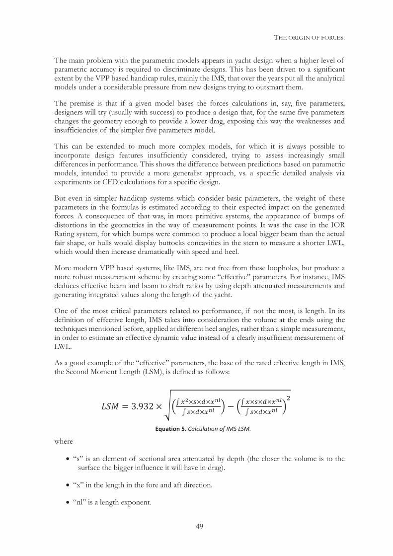
THE ORIGIN OF FORCES.
49
The main problem with the parametric models appears in yacht design when a higher level of parametric accuracy is required to discriminate designs. This has been driven to a significant extent by the VPP based handicap rules, mainly the IMS, that over the years put all the analytical models under a considerable pressure from new designs trying to outsmart them.
The premise is that if a given model bases the forces calculations in, say, five parameters, designers will try (usually with success) to produce a design that, for the same five parameters changes the geometry enough to provide a lower drag, exposing this way the weaknesses and insufficiencies of the simpler five parameters model.
This can be extended to much more complex models, for which it is always possible to incorporate design features insufficiently considered, trying to assess increasingly small differences in performance. This shows the difference between predictions based on parametric models, intended to provide a more generalist approach, vs. a specific detailed analysis via experiments or CFD calculations for a specific design.
But even in simpler handicap systems which consider basic parameters, the weight of these parameters in the formulas is estimated according to their expected impact on the generated forces. A consequence of that was, in more primitive systems, the appearance of bumps of distortions in the geometries in the way of measurement points. It was the case in the IOR Rating system, for which bumps were common to produce a local bigger beam than the actual fair shape, or hulls would display buttocks concavities in the stern to measure a shorter LWL, which would then increase dramatically with speed and heel.
More modern VPP based systems, like IMS, are not free from these loopholes, but produce a more robust measurement scheme by creating some “effective” parameters. For instance, IMS deduces effective beam and beam to draft ratios by using depth attenuated measurements and generating integrated values along the length of the yacht.
One of the most critical parameters related to performance, if not the most, is length. In its definition of effective length, IMS takes into consideration the volume at the ends using the techniques mentioned before, applied at different heel angles, rather than a simple measurement, in order to estimate an effective dynamic value instead of a clearly insufficient measurement of LWL.
As a good example of the “effective” parameters, the base of the rated effective length in IMS, the Second Moment Length (LSM), is defined as follows:
where
“s” is an element of sectional area attenuated by depth (the closer the volume is to the surface the bigger influence it will have in drag).
“x” in the length in the fore and aft direction.
“nl” is a length exponent.
Equation 5. Calculation of IMS LSM.
THE ORIGIN OF FORCES
50
The depth attenuation of sectional areas is performed by multiplying each Z (vertical offset) by e (-10 x Z/LSMO).
The final effective length used by the IMS program is the result of averaging LSMs calculated for sailing trim with 0 and 25 degrees of heel, as well as a “sunk” condition with 0 degrees of heel but with a forced extra immersion (to deal with “artificially raised” overhang trying to “cheat” the handicap system).
This gives an idea about how complex the definition of these parameters can be, and clearly it justifies the convenience of integrating a Lines Processing Program (LPP) in any serious performance prediction code, so that it is possible to generate and measure additional parameters to what a standard hydrostatic calculation would provide. These effective parameters are used not only to avoid hard measurement points and loophole abuse in handicap systems, but also to find new parameters which may show an improved correlation with the calculated forces for a variety of designs.
Just to give a non-exhaustive list of possible parameters which can be used to characterize a yacht’s hull geometry, the following traditional ones could be considered:
Length Overall Waterplane Area Amidships Coefficient Waterplane Coefficient Length Waterline Side Area Prismatic Coefficient Long. Center of Buoyancy Beam Waterline Maximum Section Area Block Coefficient Vertical Center of Buoyancy Hull Draft Hull Volume Side Area Coefficient Long. Center of Flotation
In addition to those, some types of boats require additional parameters. Amongst them, we can find some such as:
Effective/Integrated Lengths Beam at the stern Local Prismatic Coefficients Effective/Integrated Beams Immersed transom area Weighted Centers of Buoyancy Effective/Integrated Drafts Transom immersion Overhangs lengths Transom Deadrise Angle Overhangs angles
Specific designs (for instance, with or without an immersed transom) may require specific parameters which may have little relevance for other designs.
In addition to this, all the previous parameters can be calculated for different flotations with varying values of displacement, heel or trim angles.
It is interesting to note that sometimes it is possible to describe mathematically the whole hull geometry with less amount of data than the collection of parameters listed above.
The final aim for scientists and engineers is to be able to describe the physical phenomena dependent on that geometry with a model that uses the smallest possible number of those parameters. To achieve that, it is necessary to have a qualitative knowledge of the phenomena to be modeled, in order to know which parameters it will depend on, and a quantitative one in order to evaluate their individual effects.
In the next paragraphs, some examples of parametrization in force models will be given to provide some insight on this technique.
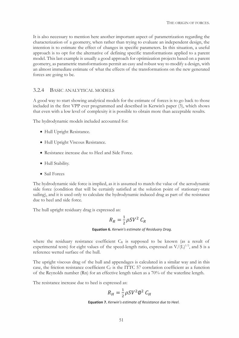
THE ORIGIN OF FORCES.
51
It is also necessary to mention here another important aspect of parametrization regarding the characterization of a geometry, when rather than trying to evaluate an independent design, the intention is to estimate the effect of changes in specific parameters. In this situation, a useful approach is to opt for the alternative of defining specific transformations applied to a parent model. This last example is usually a good approach for optimization projects based on a parent geometry, as parametric transformations permit an easy and robust way to modify a design, with an almost immediate estimate of what the effects of the transformations on the new generated forces are going to be.
3.2.4 BASIC ANALYTICAL MODELS
A good way to start showing analytical models for the estimate of forces is to go back to those included in the first VPP ever programmed and described in Kerwin’s paper (3), which shows that even with a low level of complexity it is possible to obtain more than acceptable results.
The hydrodynamic models included accounted for:
Hull Upright Resistance.
Hull Upright Viscous Resistance.
Resistance increase due to Heel and Side Force.
Hull Stability.
Sail Forces
The hydrodynamic side force is implied, as it is assumed to match the value of the aerodynamic side force (condition that will be certainly satisfied at the solution point of stationary-state sailing), and it is used only to calculate the hydrodynamic induced drag as part of the resistance due to heel and side force.
The hull upright residuary drag is expressed as:
where the residuary resistance coefficient CR is supposed to be known (as a result of experimental tests) for eight values of the speed-length ratio, expressed as V/(L)1/2, and S is a reference wetted surface of the hull.
The upright viscous drag of the hull and appendages is calculated in a similar way and in this case, the friction resistance coefficient CF is the ITTC 57 correlation coefficient as a function of the Reynolds number (Rn) for an effective length taken as a 70% of the waterline length.
The resistance increase due to heel is expressed as:
Equation 6. Kerwin's estimate of Residuary Drag.
Equation 7. Kerwin's estimate of Resistance due to Heel.
THE ORIGIN OF FORCES
52
where there is a static dependency on the squared heel angle and also on the coefficient CH, which may have a linear or parabolic dependency on the Froude number with the possible addition of higher power of heel angle.
The resistance increase due to the side force is easily identified as induced drag and as such is principally a function of the effective aspect ratio of the hull-keel combination and the square of the side force, thus looking like this:
where FH is the side force and CI is an induced drag coefficient, dependent on heel and on Froude number, which is suggested to be calculated by regression on the same experimental data from which the coefficients C1 and C2 must be obtained.
For the hull stability, a formula dependent on a linear hydrostatic moment, the metacentric height, heel angle and VCG is used. Additional terms provide a dependency with heel and the Froude number, to account for the effects of speed linked to heel, stability and the estimated vertical position of the hydrodynamic center of effort of the side force. Again, it is suggested to use experimental results to obtain the coefficients of those terms.
Finally, the sail forces are calculated from non-dimensional sail forces coefficients, which are functions of the apparent wind angle. The sail forces coefficients, the sail area and a correction for the aspect ratio of the sail plan are used for the final calculation of the sail forces. A simple reefing function is added to provide a depowering adjustment. It changes the sail area and reduces the vertical position of the aerodynamic center of effort.
As it can be seen, it is an open scheme that leaves room for the calculation of many coefficients via experimental regressions, or further parametric calculations based on those regressions to be applied to a wider range of designs. However, all the basics are already there, ready to add an additional layer of complexity.
3.2.5 SOME EXAMPLES OF MORE COMPLEX ANALYTICAL MODELS
There is a significant amount of published parametric models available for use in VPPs or even for a direct calculation of forces. Reproducing them is beyond the scope of this study, but as an example, some of them will be presented with the recommendation to go to the sources for more complete information.
Some good compilations are available. There exists mainly three sources that provide a good set of information, that summarize most of the efforts made in the last 30 years to model the forces involved in sailing, and that provide references to many other proposals and studies
Chronologically, the first is the Delft Systematic Series, result of a large number of models with parametric variations tested in towing tanks. Improved versions have been published over time with new added models and more accurate regressions. The development and testing of this series started back in the 1970’s with its first version published in 1980 (16), covering only hull drag in calm water. This work has been extended over the years until today (17) with a number of additional publications covering everything from resistance added in waves (18) to appendage
Equation 8. Kerwin's estimate of Resistance due to Side Force.
THE ORIGIN OF FORCES.
53
forces and improved hull regressions (19), maneuverability (20), and even consideration of the effect of trim on hull drag.
The next one is “Predicting the Speed of Sailing Yachts” published by Peter Van Oossanen in the SNAME transactions in 1992 (21), which describes in a detailed way the origin of a systematic breakdown of forces for which it proposes different analytical models. The last one is the already mentioned publication from the Offshore Racing Congress titled “ORC VPP Documentation” (8), which describes the mathematics behind the IMS VPP and its analytical models, in a significant effort by the International Technical Committee to keep an up-to-date description of the core models inside of the VPP.
But moving to discuss specific models, we will start by taking the calculation of residuary drag as a reference. We will start with a simple model used by G. Hazen (22) in one of the most advanced implementations of an “IMS like” VPP programmed in the late 80’s.
This model proposes the following formula for the calculation of the Residuary Drag:
Where CV is the volumetric coefficient expressed as (L/ (1/3)), the displacement in pounds, B the beam waterline and T the hull draft. A table of the coefficients a, b and c is provided for 8 values of V/(LSM)1/2 between 0.4 and 0.8.
That formulation provides a source of forces for the residuary drag, that can be used for different geometries, and which takes into account the main hull parameters influencing the generation of drag (length, beam, draft and displacement). Obviously, improvements are possible and they certainly happened, as the next example will show, but this was a good step forward trying to take into account boat parameters for generalized models, from the original simple Kerwin regression (3).
The modern version of a parametric model for the calculation of the hull Residuary Drag can be found in the Delft Systematic Yacht Hull Series (DSYHS). This series, up until its third edition provided one model for Froude numbers up to 0.45 and a different one for the range between 0.45 and 0.6.
Equation 9. Hazen's original Residuary Drag calculation.
Equation 10. DSYHS Residuary Drag calculation.
THE ORIGIN OF FORCES
54
In the last version, the two separate models were unified, to cover the full range of Froude Numbers between 0.1 and 0.6, in the expression shown as Equation 10.
The coefficients A1 to A8 are provided in a table for values of Froude Number of 0.10, 0.15, 0.20, 0.25, 0.30, 0.35, 0.40, 0.45, 0.50, 0.55 and 0.60. Residuary Drag for specific values must be interpolated.
This formula gives an idea of the complexity a parametric model can reach, the number of hull models tests required and the parameters the creators of the Series estimated to be relevant to the generation of the residuary drag.
An interesting case happened in the IMS in 2013, when the residuary drag model was replaced by a simpler one, of characteristics similar to the Delft Series model, but specially adapted to the modern Offshore Sailing Yachts shapes. This new model made more emphasis in the calculation of the effective lengths for a number of sailing conditions, but reduced the dependencies to a Dynamic Length-Volume ratio (LVR) and a Beam-Hull Draft ratio (BTR), the key coefficients. Along with this, further refinements were made in the calculation of “composite effective lengths” calculation, as the main driving parameter.
The main reason was that, despite the number of parameters used, designers still managed to find “niches” of “better than predicted” performance. As a consequence, despite the efforts to avoid it, the IMS handicap system had an undesired type forming effect (a common problem for all handicap systems) that was seen by many as promoting slower yachts. By trying to make the best possible evaluation of a fundamental source of drag, IMS has left too many doors open for exploitation.
Going back to the Delft Series, although the original DSYHS was limited to hulls, and drag for upright tests in flat water, new models have been incorporated, as well as models tested with appendages. That is the reason why it provides today a range of parametric models that cover most of the hydrodynamic forces.
Sometimes, the parametric models are used as well to estimate some of the required geometric information based on simpler parameters. An example is the formula from the DSYHS, providing an estimate of the wetted surface of the hull based on basic hull parameters, as follows:
Obviously, nowadays the actual wetted surface can be easily calculated, but this shows that no matter how basic the definition available for a design, “some” kind of performance prediction can be done.
In addition to the bare-hull residuary and viscous drag, the DYSHS also provides parametric models for the calculation of changes in both resistances due to heel and to longitudinal changes in trim. For appendages, force predictions are provided for viscous, induced and even residuary resistances (due to the keel proximity to the free surface), as well as corrections for heel.
Equation 11. DSYHS estimate of the hull wetted surface.
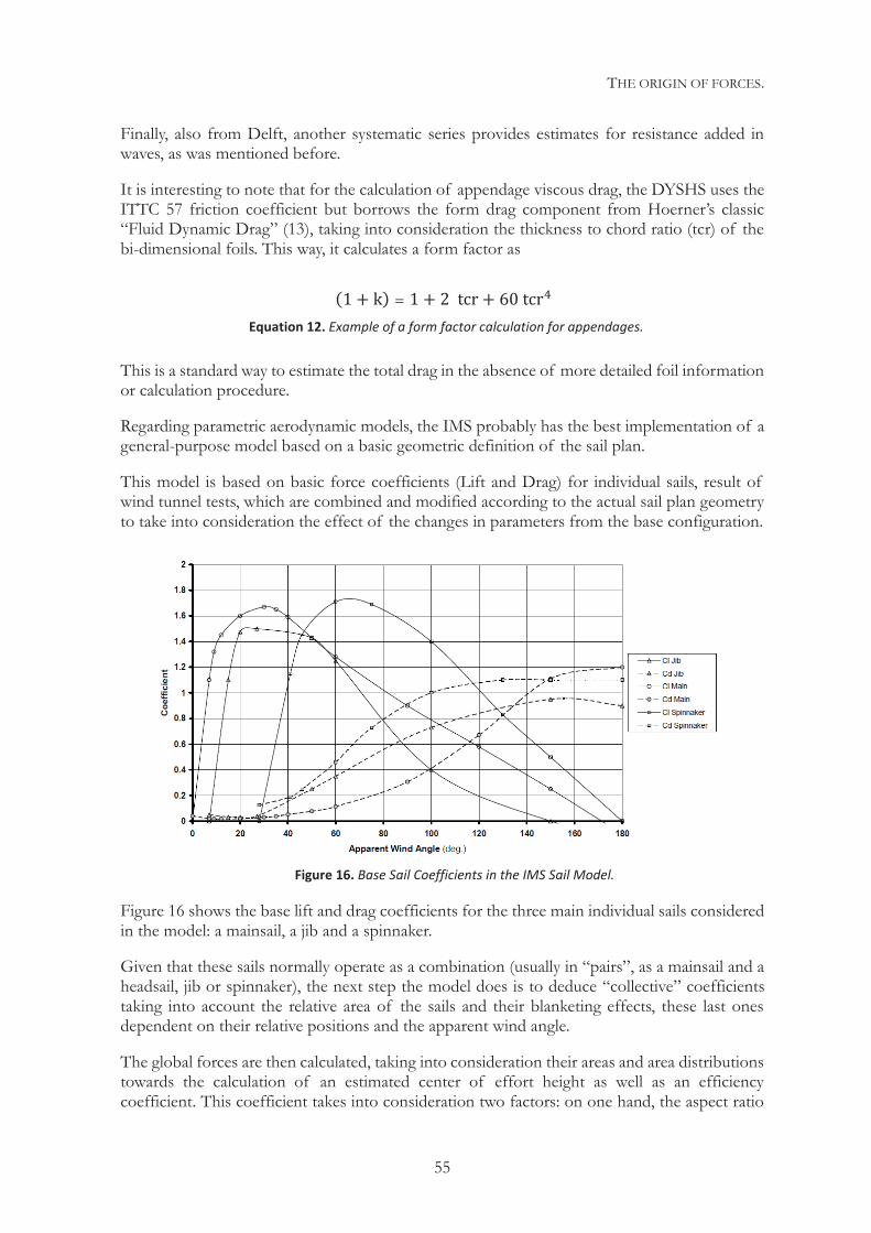
THE ORIGIN OF FORCES.
55
Finally, also from Delft, another systematic series provides estimates for resistance added in waves, as was mentioned before.
It is interesting to note that for the calculation of appendage viscous drag, the DYSHS uses the ITTC 57 friction coefficient but borrows the form drag component from Hoerner’s classic “Fluid Dynamic Drag” (13), taking into consideration the thickness to chord ratio (tcr) of the bi-dimensional foils. This way, it calculates a form factor as
This is a standard way to estimate the total drag in the absence of more detailed foil information or calculation procedure.
Regarding parametric aerodynamic models, the IMS probably has the best implementation of a general-purpose model based on a basic geometric definition of the sail plan.
This model is based on basic force coefficients (Lift and Drag) for individual sails, result of wind tunnel tests, which are combined and modified according to the actual sail plan geometry to take into consideration the effect of the changes in parameters from the base configuration.
Figure 16 shows the base lift and drag coefficients for the three main individual sails considered in the model: a mainsail, a jib and a spinnaker.
Given that these sails normally operate as a combination (usually in “pairs”, as a mainsail and a headsail, jib or spinnaker), the next step the model does is to deduce “collective” coefficients taking into account the relative area of the sails and their blanketing effects, these last ones dependent on their relative positions and the apparent wind angle.
The global forces are then calculated, taking into consideration their areas and area distributions towards the calculation of an estimated center of effort height as well as an efficiency coefficient. This coefficient takes into consideration two factors: on one hand, the aspect ratio
Equation 12. Example of a form factor calculation for appendages.
Figure 16. Base Sail Coefficients in the IMS Sail Model.
THE ORIGIN OF FORCES
56
of the sail plan for the calculation of the induced drag, and on the other hand the increase in viscous drag with lift, which assumes a proportional increase in separation.
On top of this, a depowering scheme is provided. This was originally limited to the traditional reef and flat parameters, with “reef ” reproducing the effects or mainsail reefing (reduction of sail area, aspect ratio and height of center of effort) and “flat” reproducing the effect of reducing camber in sails (reducing the lift coefficient and viscous drag associated with lift). The optimum combination would then be searched by the IMS VPP to maximize performance.
Nowadays, depowering is performed in a way that reproduces in a more realistic way the normal process which happens in a sailing yacht when the wind increases (10).
A degree of “twist” has been associated to the “flat” parameter, which now also lowers the center of effort. In addition, the original “reef ” parameter has been replaced by two others, which first reduce the foot length of the headsail until the minimum size has been reached (and the new “collective” coefficients based on the new sail ratios are recalculated iteratively), and then the mainsail is “reefed” in the traditional way.
These are just some specific examples, but it is possible to find in the cited references parametric models for virtually any source of forces, and certainly to provide a more than sufficient base for a general-purpose VPP.
STRATEGY IDENTIFYING SOURCES OF FORCES One of the main ideas to keep in mind from this Chapter is to always remember how difficult it can be to calculate some of the forces, and how important this makes being able to identify properly what their origin might be.
This importance goes to the basic fact of deciding which methods will be used to estimate the forces. This may have an impact on what the value of those calculated forces will be.
It is not possible to make any accurate performance assessment for a sailing yacht without properly understanding the nature of the problem and the fact that making simplifications does not necessarily degrade the quality of the solution. There is an adequate scientific reason behind those simplifications, and their effect can be quantified.
Sailing Yachts, given the already discussed nature of their motions and the number of coupled effects involved in them, require a proper view of the “big picture” of the problem. As with numerical analysis, it is easy to obtain a reasonable solution that is completely wrong when an underlying understanding of the physics of the global problem is not present.
In addition, the fact is that whichever deconstruction of forces is made conceptually, different alternatives are possible.
For instance, when there is a phenomenon of separation in the boundary layer of a lifting element, there is an increase of the generated drag and a degradation of lift. In this case, the division between the strictly potential phenomena and the part of them which is derived from viscosity is not that clear. When obtaining experimental results in this situation, for instance, the changes in drag from the ideal situation can be modeled as a separate “force modifier”, or alternatively by splitting the induced drag in two different components: one depending on the
THE ORIGIN OF FORCES.
57
linear lift and the other on the non linear lift (not unusual in low aspect ratio bodies generating lift, even with fully attached flow).
The influence of viscosity adds additional complications when trying to clear distinctions between the causes of forces. That is not surprising, considering that in an attached flow, in which the level of viscosity has no influence on the generation of lift, its very existence is required for the lift to be produced.
A similar difficulty arises when considering the effect of interference between different elements. A visible case (literally) happens when, due to the heel angle, a keel generating a side force is close to the free surface affecting it. This has a consequence on the end plate effect the hull has on the keel, and therefore on its effective span but it also alters the wave pattern and wetted surface of the hull. In addition, some measurable influence on the stability may even happen.
This is just an example of how complex interactions can get and the impact it can have when trying to perform an actual calculation of the individual forces.
In the case of VPP based handicap systems, simplifications take over as a necessary evil when trying to deal with a wide range of designs.
When the use of the VPP is intended to evaluate and improve a given design, it is important to concentrate the biggest detail of the models on those primarily affected by the parameters to be optimized or evaluated.
Since most of the VPP work involves an objective comparison, experience shows that systematic known errors (which could be assumed as systematic known simplifications) are preferable to having different levels of them, especially when they are hard to quantify.
When discussing VPP solutions, some examples of bad results for inconsistent calculation strategies will be given.
In the next Chapter, the discussion will be more oriented to tools that in general will provide global forces, rather than a detailed breakdown of them. It is tempting to assume that this will make the detailed calculations irrelevant, but such assumption would be a mistake.
Most optimizations are not global, but focused on specific aspects of design, and as such, having a good global information on a base design is almost a necessity in order to make detailed studies on “sub-systems” like, for instance, a rudder. It is necessary then to have the possibility to assess how the global forces will be affected by these “local” changes. To do this, it is required to quantify the effect of some parameters changes for which the analytical calculations are very accurate, to then substitute their effect on the global forces.
The efficient use of resources is vital, and having a computer running 5 days of calculations for something that could be estimated in a few hours, sometimes in a more accurate way, is clearly bad engineering. This is where a good global knowledge of the problem to be solved helps to define the strategy to acquire the best set of data for a performance prediction with the available resources.
Once again, it all points to well-educated scientific “common sense”.

THE ORIGIN OF FORCES
58
This page intentionally left blank
EVALUATING FORCES WITH EMPIRICAL AND NUMERICAL TOOLS
59
4| EVALUATING FORCES WITH EMPIRICAL AND NUMERICAL TOOLS
Up to this point, the generation of forces and the basic equilibrium have been discussed. In addition, some generic methods based on analytical models or basic theoretical deductions have been suggested to evaluate the individual forces towards a global equilibrium calculation.
At the same time, the complex interaction mechanisms between the different forces have been exposed. They explain the interest in finding ways to directly obtain global forces, bypassing the complications and errors derived from making simplifications while managing those interactions.
In order to obtain these global forces, the two main available alternatives are experimental and numerical data. However, even with these methods, in most cases it will be necessary to understand how forces are generated in order to obtain the global full-scale ones.
The numerical codes have been available almost since the appearance of computers (although many of their theoretical bases had already been established before that). Different techniques have been used for the discretization and solution of the problems. They present different challenges in terms of reliability, accuracy and robustness, and different requirements in computational power. Nowadays, numerical codes are a tool of rapidly increasing importance when predicting performance.
On the experimental side, the first tools to ever be used were the towing tanks (also known as ship model basins). In these facilities, experiments are performed by towing scaled down models in a long pool, while measuring the hydrodynamic forces generated. Similarly, wind tunnels have been used to determine aerodynamic forces on sail plans, exposed structures and even as a way to calculate hydrodynamic forces in some lifting elements. Although they play a key role in the creation of analytical sail models, they are less common as a tool regularly used for performance prediction (collecting data for a specific design). Given this fact, they will be discussed in less depth than the towing tanks. For these two experimental tools, the scale factor used in the construction of the models is responsible for the main layer of difficulty and uncertainty associated with the process of extrapolating the viscous forces to full scale
In addition to the normal use of sailing data from the actual yacht (which at times can be very detailed), another source of experimental data is the exhaustive collection of information while sailing in fully instrumented prototypes, designed with this specific purpose. Although not a common tool, a number of these prototypes have been built and tested in the last 30 years for an even more accurate and detailed collection of data when sailing. This detailed data is then compared to the results of other calculations for the prototype, in order to perform validations or to create/tune sail models. Some of these prototypes have been discussed in detail in a number of publications, and in most cases, they are related to universities and research centers that use them regularly as a tool for different validation projects. There have been some of these, also called full-scale sailing dynamometers, in the USA (23), Japan (24), Germany (25), Italy (26) and France within the 28th America’s Cup campaign in 1992.
This last example of source for experimental data is just briefly mentioned in this introduction, as it does not belong to the toolbox of standard procedures to obtain data with the purpose of performance prediction.
EVALUATING FORCES WITH EMPIRICAL AND NUMERICAL TOOLS
60
All these methods have in common the fact that none of them is cheap, neither in terms of cost nor of time and/or requirements for specific resources.
As a consequence, their use has to be carefully planned, with a wise definition regarding what is the best data (not just in terms of accuracy but also in terms of amount of data) that can be obtained with an efficient use of the available experimental and numerical tools. These two types of resources are often used simultaneously.
In this Chapter, procedures and precautions to achieve this objective will be discussed, trying to collect the best possible information about the studied phenomena. All this will be done with the objective of making a good performance prediction.
The implications of this objective, as opposed to a more general research oriented to increase the knowledge of the physics involved, are not irrelevant, as we will see below and in the next Chapter.
A BRIEF DISCUSSION ON DESIGN OF EXPERIMENTS AND MANAGEMENT OF NUMERICAL AND EXPERIMENTAL DATA
The discussion about this topic is important by itself, but it will happen in detail in the next Chapter. However, it is necessary to anticipate some brief notes regarding how experimental and numerical data are used, and how to plan the experiments and numerical studies providing the data.
The first point to bring up is the fact that, prior to the execution of any of the methods described in this Chapter, it is necessary to define what data is required, how much of it, and with what level of detail and accuracy.
As it was mentioned before, empirical and numerical tools are expensive (at the very least, in time). For that reason, defining the minimum set of data that is going to describe the forces generated, in a way appropriate for the VPP, becomes paramount.
A good knowledge of the available tools, along with their limitations to calculate those forces, is also an important part of this process. For instance, some numerical codes used for specific calculations do not provide accurate and/or reliable results in terms of absolute numbers. However, with some cautions, it is possible to have a good measure of the relative impact of some parametric variations. That is a useful resource and result.
Additionally, the final use of the data needs to be taken into account, in order to balance the cost of the extra accuracy. This may be required in high competition but may be excessive when trying to provide reasonable polar curves for a cruising yacht.
Regarding the amount of data, depending on the source, some data points may be redundant yet convenient as a way to provide crosschecks on the data quality, but in general, knowing the forces involved will reduce the number of “gaps to be filled” (as opposed to collecting a dense cloud of data). Some parametric relationships should be known in advance and, for instance, there is little interest in obtaining forces for a high number of values of a given parameter known to have a linear behavior. In summary, the less ambiguity there is about the forces to be calculated, the less data points will be needed to characterize them.
EVALUATING FORCES WITH EMPIRICAL AND NUMERICAL TOOLS
61
Being able to anticipate in which range of parameters the performance will be predicted and where the expected solutions will yield may also help to significantly reduce the amount of required data. The type of prediction to perform (like the calculation of stationary solution vs. a time-domain analysis) will also condition how big a range will need to be covered (and the accuracy throughout it).
Data points will be structured in multi-dimensional matrices, which can be rectangular or not, can have all or just some of their elements filled, and can use different densities and number of values for each parameter. These parameters will reflect variations in the environmental conditions (water and air speeds and angles) and, in most cases, some boat adjustments that may affect performance (like a depowering factor or a rudder angle).
It is not uncommon to use more than one of the methods discussed in this Chapter for a single project. In that case, the objective is to obtain the benefits of the different tools. Most likely, the different methods will use different matrices of points. The matrices will also be different from those that would be considered necessary if only one method was available.
As stated before, the next Chapter will be dedicated to a much more detailed analysis of the data itself. However, the intention of the above points is to set some basic justification for how experiments and numerical studies are performed to obtain forces (and sometimes movements).
TYPES OF EXPERIMENTAL TESTS Many different types of tests can be performed to measure forces in a sailing yacht. Some are used much more commonly than others for performance prediction, and those are the ones we will focus on in this Chapter. Full-scale tests or fully instrumented sailing prototypes will not be discussed at this point for the reasons explained in the introduction.
The first type of test to consider is the one performed by towing a scaled down model in a calm water towing tank at a given speed. Forces, moments and movements are then measured and recorded for post-processing. The model can have appendages installed or not, and the processing of the measurements involves non-trivial scale effects to be discussed later.
This is a common way to evaluate hulls mostly, but it can also be used to evaluate appendage configurations. It is the preferred experimental tool when the potential effects (or at least their uncertainties compared to those of the rest of the forces) are dominant. This is the case, in most situations, with hulls or appendages when lift is present.
The method normally used to test sailing yachts was established a long time ago, and it is described by Professor Davidson in his paper from 1936 (1). The quality of the results relies strongly on the equipment, and largely on the expertise and attention to detail of the professionals conducting the experiments.
Sometimes tests in waves are performed but they are less common than calm water tests. Given their complexity, they tend to be limited to estimating the differences in the influence of waves on added resistance, for some models with distinctive differences or specific features (like a type of bow shape).
Maneuverability tests are another type of experiments that falls in a similar category, being normally performed for specific maneuverability studies rather than general performance prediction.
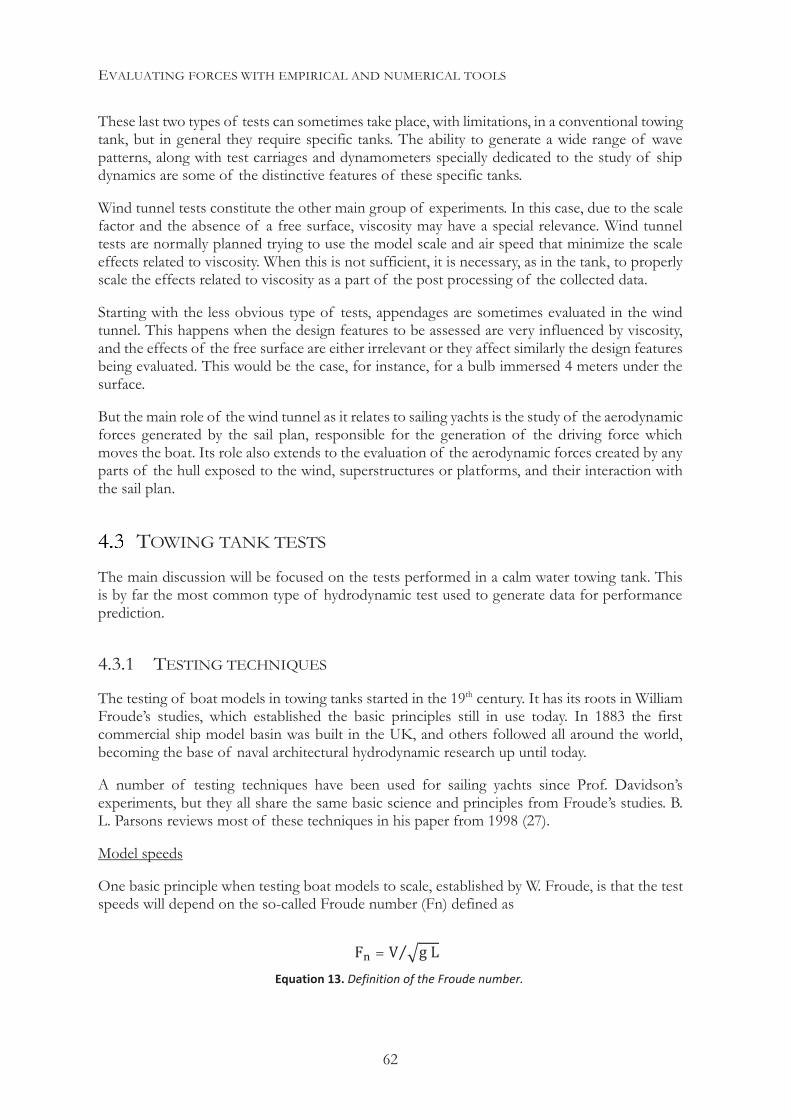
EVALUATING FORCES WITH EMPIRICAL AND NUMERICAL TOOLS
62
These last two types of tests can sometimes take place, with limitations, in a conventional towing tank, but in general they require specific tanks. The ability to generate a wide range of wave patterns, along with test carriages and dynamometers specially dedicated to the study of ship dynamics are some of the distinctive features of these specific tanks.
Wind tunnel tests constitute the other main group of experiments. In this case, due to the scale factor and the absence of a free surface, viscosity may have a special relevance. Wind tunnel tests are normally planned trying to use the model scale and air speed that minimize the scale effects related to viscosity. When this is not sufficient, it is necessary, as in the tank, to properly scale the effects related to viscosity as a part of the post processing of the collected data.
Starting with the less obvious type of tests, appendages are sometimes evaluated in the wind tunnel. This happens when the design features to be assessed are very influenced by viscosity, and the effects of the free surface are either irrelevant or they affect similarly the design features being evaluated. This would be the case, for instance, for a bulb immersed 4 meters under the surface.
But the main role of the wind tunnel as it relates to sailing yachts is the study of the aerodynamic forces generated by the sail plan, responsible for the generation of the driving force which moves the boat. Its role also extends to the evaluation of the aerodynamic forces created by any parts of the hull exposed to the wind, superstructures or platforms, and their interaction with the sail plan.
TOWING TANK TESTS The main discussion will be focused on the tests performed in a calm water towing tank. This is by far the most common type of hydrodynamic test used to generate data for performance prediction.
4.3.1 TESTING TECHNIQUES
The testing of boat models in towing tanks started in the 19th century. It has its roots in William Froude’s studies, which established the basic principles still in use today. In 1883 the first commercial ship model basin was built in the UK, and others followed all around the world, becoming the base of naval architectural hydrodynamic research up until today.
A number of testing techniques have been used for sailing yachts since Prof. Davidson’s experiments, but they all share the same basic science and principles from Froude’s studies. B. L. Parsons reviews most of these techniques in his paper from 1998 (27).
Model speeds
One basic principle when testing boat models to scale, established by W. Froude, is that the test speeds will depend on the so-called Froude number (Fn) defined as
Equation 13. Definition of the Froude number.
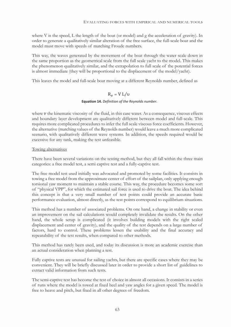
EVALUATING FORCES WITH EMPIRICAL AND NUMERICAL TOOLS
63
where V is the speed, L the length of the boat (or model) and g the acceleration of gravity). In order to generate a qualitatively similar alteration of the free surface, the full-scale boat and the model must move with speeds of matching Froude numbers.
This way, the waves generated by the movement of the boat through the water scale down in the same proportion as the geometrical scale from the full scale yacht to the model. This makes the phenomenon qualitatively similar, and the extrapolation to full scale of the potential forces is almost immediate (they will be proportional to the displacement of the model/yacht).
This leaves the model and full-scale boat moving at a different Reynolds number, defined as
where the kinematic viscosity of the fluid, in this case water. As a consequence, viscous effects and boundary layer development are qualitatively different between model and full-scale. This requires more complicated procedures to infer the full scale viscous force coefficients. However, the alternative (matching values of the Reynolds number) would leave a much more complicated scenario, with qualitatively different wave systems. In addition, the speeds required would be excessive for any tank, making the test unfeasible.
Towing alternatives
There have been several variations on the testing method, but they all fall within the three main categories: a free model test, a semi captive test and a fully-captive test.
The free model test used initially was advocated and promoted by some facilities. It consists in towing a free model from the approximate center of effort of the sailplan, only applying enough torsional yaw moment to maintain a stable course. This way, the procedure becomes some sort of “physical VPP”, for which the estimated sail force is used to drive the boat. The idea behind this concept is that a very small number of test points could provide an accurate basic performance evaluation, almost directly, as the test points correspond to equilibrium situations.
This method has a number of associated problems. On one hand, a change in stability or even an improvement on the sail calculations would completely invalidate the results. On the other hand, the whole setup is complicated (it involves building models with the right scaled displacement and center of gravity), and the quality of the test depends on a large number of factors, hard to control. These problems lessen the usability and the final accuracy and repeatability of the test results, when compared to other methods.
This method has rarely been used, and today its discussion is more an academic exercise than an actual consideration when planning a test.
Fully captive tests are unusual for sailing yachts, but there are specific cases where they may be convenient. They will be briefly discussed later in order to provide a short list of guidelines to extract valid information from such tests.
The semi-captive test has become the test of choice in almost all occasions. It consists in a series of runs where the model is towed at fixed heel and yaw angles for a given speed. The model is free to heave and pitch, but fixed in all other degrees of freedom.
Equation 14. Definition of the Reynolds number.
EVALUATING FORCES WITH EMPIRICAL AND NUMERICAL TOOLS
64
Given that the boat is towed from a point situated at a height lower than the center of effort of the sail plan, it is necessary to replace the missing pitch moment that the driving force would induce (due to the difference in the moment arm) with an additional pitch moment. This is accomplished by moving weights longitudinally, based on an estimated drag (and thus, required driving force). In addition, when heel is present, the resulting vertical component of the sail force needs to be simulated by adding of weight to the model. If the estimates used for the weight calculations prove to have a significant error, they can be corrected and the points retested.
These two necessary corrections and input to the test setup, point to the importance of having suitably accurate estimates of the results before carrying out the tests.
In this testing technique, the forces and moments in the restricted degrees of freedom are measured, and the motions in the free ones are recorded. Special four-six degrees of freedom dynamometers are required. The following discussion will focus on this test method, which is by far the most used for monohulls, and in general for yachts where pitch and heave stability is not critical. When pitch and heave stability are critical, for instance when there are sailing points with no stable equilibrium, alternative setups might need to be considered.
4.3.2 REPEATABILITY AND ACCURACY
The concept of repeatability has been mentioned briefly before but it is necessary to stress its importance.
Repeatability is a self-explanatory concept and it is used to estimate the uncertainty of the experiment. It designates the ability to reproduce the measured results when the same model is tested at different times in the same test conditions and parameters (or providing corrections for environmental changes such as tank water temperature). Although being able to reproduce a test result may sound like a trivial task, it represents a challenge in tank tests and especially in the case of sailing yachts, due to a series of added complications.
As of today, the best sailing yacht tank tests can discriminate drag differences under 0.5%, meaning that repeatability must be better than that 0.5%. These levels of quality are achieved at probably just two or three facilities around the world, and are the result of exceptional attention to detail and understanding of the test problems by test specialists. Not only the test equipment, but also the test procedures and personnel expertise are determinant in making the tank test a powerful tool for performance prediction, rather than a tool producing a set of results that are only correct in appearance. Repeatability represents a good measure of the level of accuracy that a facility is able to achieve with its testing procedures.
Also important is the need for accuracy in the measurements, meaning that the results correspond exactly to the forces produced during the test. To achieve this, the effects of external influences must be minimized, to avoid adding limitations to those implicit in the measurement system itself.
In the next sections, a number of factors that can be the source of problems and inaccuracies will be described. As well, precautions to avoid their negative impact on the results will be proposed. These are related more to tank test techniques than to performance prediction, but awareness of these problems teaches that tank data must be questioned and carefully evaluated for quality, starting with the tank testing process itself.
EVALUATING FORCES WITH EMPIRICAL AND NUMERICAL TOOLS
65
4.3.3 THE MODELS
The first potential cause of inaccuracies is in the models themselves. This involves the accuracy of the geometry, weight, surface finishing and turbulence stimulation.
Model design and construction
The first parameter to be decided when planning a tank test is the scale of the models. The larger the models, the less uncertainty in viscous effects will exist, and in general the smaller the relative errors will be. For this reason, the model scale will be determined (other than by cost) by the largest model that can be tested in the facility, given the dimensions of the tank section (to avoid blockage effects due to interference with the walls), maximum test speeds and tank length. All of these factors are related to each other.
In addition, the expected forces must be within the dynamometer specifications, ensuring that:
They fit the range of calibration of the load cells and stay below the maximum loads that they can withstand.
They do not exceed the loads tolerated by the general stiffness and strength limitations of the dynamometer, the model attachment system and the towing carriage.
The best facilities used in America’s Cup test programs have tank basins in excess of 200 meters long, around 12 meters wide and an approximate depth of 6 meters. The test carriages are capable of speeds up to 10 meters/second.
While larger and faster facilities are available, academic facilities with dimensions around 1/3 of those described above can also be a source of data (mostly for parametric studies, and obviously with a significant lower accuracy and repeatability, but also lower cost).
The model geometry must correspond to the design, and the construction needs to be stable in shape, both under the normal loads and the environmental conditions it will be exposed to. Templates and tools must be provided to verify this after construction.
If the models (or parts) are built in a CNC milling machine, reference points must be marked in different places, as part of the milling process, in order to facilitate future checks. Some of the check points must be placed on deck, at both sides and along the length (3+3 is a reasonable arrangement), for torsion and bending verifications.
References for the internal structure to be attached to the dynamometer and the appendages attachment area (sometimes and ideally the same structural piece) should be marked, and if possible, drilled in place to guarantee its proper alignment.
In composite models (very common nowadays), the laminates and lamination process should be carefully designed and verified to minimize deformations during the polymerization and post curing.
The models must be properly marked, outside and inside with a common reference for the attachment to the dynamometer and appendages, as well as for setting the different test positions (depending on the setup).
The surface finish must be consistent between different models. Wet sanding with 800 to 1200 grit paper over a properly painted surface is a way to provide a repeatable surface, especially if
EVALUATING FORCES WITH EMPIRICAL AND NUMERICAL TOOLS
66
consistency in the painting process cannot be guaranteed. If sanding is required, consistent patterns must be used, in terms of grit, sequence and sanding angles, especially in the final stages. Failure to do so can lead to inconsistent results.
The model weight must be low enough to make room for ballast weight, and for its translation to obtain the required trim moments during the test process.
Finally, in order to know the location of the transition from laminar to turbulent flow, proper turbulence stimulation must be set, taking into consideration the dynamic nature of the waterline. Sometimes, overhangs can be significant, and in this case, two rows of stimulation are normally used. Conventional ITTC studs properly calculated for the range of speeds are the usual choice.
For appendages, the same stimulation studs could be used, but smaller “dot-like” devices placed with a higher density, inspired from those used on wings in wind tunnels, have shown a more consistent behavior for different speeds. Their height is better suited for the boundary layer thickness, given the short chord lengths and consequently low values of the Reynolds number.
Whichever the choice of stimulation, consistency is again paramount when performing comparisons.
Model integrity and verification
Before testing a model, the finalized geometry must be verified. This can be done with carefully chosen templates. But it is just as important to confirm that the model geometry is stable, and that no hogging, sagging or torsional deformations have appeared.
A simple verification using the deck height reference points should be made before starting the test, with the model in the water and the dynamometer installed. If there are concerns regarding deformations, they should be evaluated in the same manner right after the test has been finished.
It is also necessary to regularly inspect the turbulence stimulators to verify that their integrity is maintained throughout the test session.
One important aspect regarding model accuracy is the correct alignment between the hull and appendages (and between different appendages), which will rely, as a starting point, on the symmetry of the construction and on attachments and their positioning. However, the final evaluation is of a functional nature, and will also be discussed when talking about the model setup in the next section.
Finally, the weight of the boat must be carefully monitored. It is not unusual to find a situation in which the model has taken water and displacement has increased, to a point which may render the results useless.
If the result of the above verifications is positive, a first step towards repeatability and accuracy has been completed.
Often, small violations in those verifications happen. Then sensitivity tests should be run to evaluate the impact on the final results, basically in the performance prediction based on the data obtained.
Depending on the importance of the effects, their influence can be ignored, corrections applied, or measures taken, for example to restore an excessive deformation of the model.
EVALUATING FORCES WITH EMPIRICAL AND NUMERICAL TOOLS
67
It is important to remember that a tank test is not a basic science experiment, but a tool intended to assess performance. Therefore, knowing the importance of a deviation from perfection is key to determining which factors can influence the results or not.
This is one of the reasons why in high performance projects it is not uncommon for the person in charge of the final performance prediction to work closely with the tank expert, given that at times, important agreed decisions must be taken during the normal development of the test.
4.3.4 THE MODEL SETUP, DYNAMOMETER AND DATA ACQUISITION SYSTEMS
The dynamometer is a key component of the test, first because it is responsible for measuring the forces, but also because it sets the position and motion constraints of the model.
Model attachment and movements
Every tank has its own setup, but normally the dynamometer and the model attachment systems, which constrain or allow movement in different degrees of freedom, are part of the same system.
This system (attachment system, test carriage, etc.) must be stiff enough to guarantee that the desired testing position is maintained when forces are generated, while allowing a friction-free movement in heave and pitch under load. This can sometimes be verified under load, with the carriage moving, by applying forces and measuring the movements that they cause.
The other source of movement is the speed of the carriage towing the model, and it should be accurate and stable. Usually, an independent speed measurement system using encoders provides feedback to the control system. It is important to note that results should be analyzed using the speed measured over time during a run, rather than the input speed.
A speed control system providing the ability to define specific acceleration and deceleration ramps allows to maximize the usable length of the tank where the model moves in a steady condition.
A problem related to the phase of acceleration is the transient oscillation motion generated when starting the run because the model is towed from a point higher than the center of the hydrodynamic forces. This pitch oscillation has a period dependent on the pitch inertia of the ballasted model, and it normally damps itself so that the model reaches a stationary state. A carefully designed acceleration profile for each speed, depending on the natural pitching period, can help to reduce significantly this oscillation or even virtually eliminate it.
One important check, with the model fitted with appendages, is the alignment with the direction of movement. It should first be done with only the keel installed, doing a yaw sweep, of normally three points, and inferring the zero lift angle. This permits to verify that the keel does not have any asymmetries and has been mechanically accurately aligned with the centerline of the model. After that, a similar procedure is performed adding the rudder and setting it to find its true zero lift angle.
If some minor misalignment between the hull and appendages exists despite the care taken during the construction, this alignment procedure will limit its consequences. The procedure may have some effects in the global lift and drag, but given that the lift slope of the bare hull is
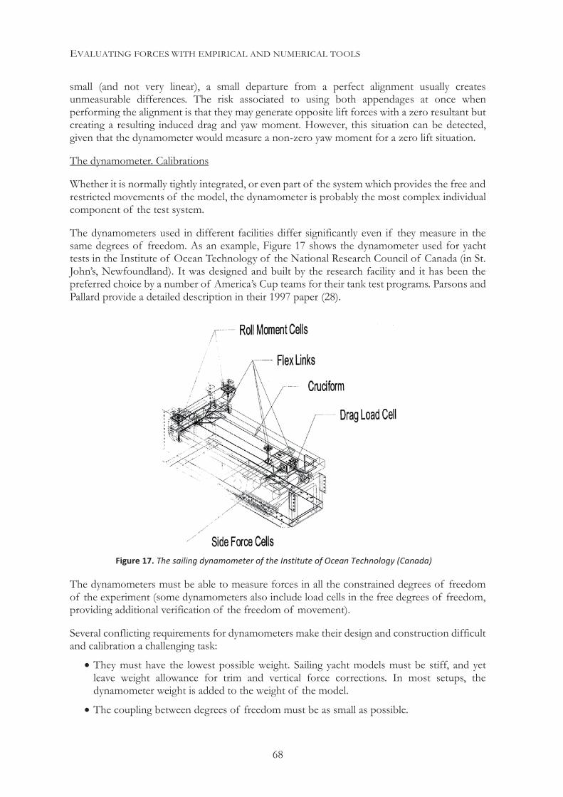
EVALUATING FORCES WITH EMPIRICAL AND NUMERICAL TOOLS
68
small (and not very linear), a small departure from a perfect alignment usually creates unmeasurable differences. The risk associated to using both appendages at once when performing the alignment is that they may generate opposite lift forces with a zero resultant but creating a resulting induced drag and yaw moment. However, this situation can be detected, given that the dynamometer would measure a non-zero yaw moment for a zero lift situation.
The dynamometer. Calibrations
Whether it is normally tightly integrated, or even part of the system which provides the free and restricted movements of the model, the dynamometer is probably the most complex individual component of the test system.
The dynamometers used in different facilities differ significantly even if they measure in the same degrees of freedom. As an example, Figure 17 shows the dynamometer used for yacht tests in the Institute of Ocean Technology of the National Research Council of Canada (in St. John’s, Newfoundland). It was designed and built by the research facility and it has been the preferred choice by a number of America’s Cup teams for their tank test programs. Parsons and Pallard provide a detailed description in their 1997 paper (28).
The dynamometers must be able to measure forces in all the constrained degrees of freedom of the experiment (some dynamometers also include load cells in the free degrees of freedom, providing additional verification of the freedom of movement).
Several conflicting requirements for dynamometers make their design and construction difficult and calibration a challenging task:
They must have the lowest possible weight. Sailing yacht models must be stiff, and yet leave weight allowance for trim and vertical force corrections. In most setups, the dynamometer weight is added to the weight of the model.
The coupling between degrees of freedom must be as small as possible.
Figure 17. The sailing dynamometer of the Institute of Ocean Technology (Canada)
EVALUATING FORCES WITH EMPIRICAL AND NUMERICAL TOOLS
69
The dynamometer geometry must be as stable as possible under load and changes of temperature.
They are subject to significant combined loads that vary in amount and distribution.
They are part of the attachment of the model to the test carriage, which must be stiff in some degrees of freedom but still allow free motions in others.
They are subject to motions with accelerations, as well as vibrations, and for some cells, to negative loads in the deceleration phase.
This can give an idea of the difficulty to perform a proper calibration, which takes place in different ways.
The first basic calibration is related to the individual load cells already in place inside the configuration. This is required to confirm and/or correct, with simple individual axial pulls, their individual calibrations (as performed for the individual cells before their integration in the dynamometer).
The next step in calibration consists in combined sets of loads, and in this situation, complexity escalates significantly, as the final purpose is to have a global calibration which includes the calculation of the crosstalk matrix. This will allow to calculate the cross influence between the different cells under load. This is unique not only for each dynamometer design but also for each individual unit, and can change over time for a number of reasons. Obviously, an unjustified significant change between verifications should raise flags and trigger a search for a satisfactory explanation.
Although dynamometers are designed to minimize the cross effects between load cells in different axis (using decoupling rods in their attachments and through a careful design of their geometries), some cross effects are always present, even if small. And they cannot be ignored, especially when the forces are not clearly dominant in one of the measuring axis.
Complete dynamometer calibrations, as described above, must be routinely performed. In addition, careful checks should be carried out when attaching the dynamometer to the carriage at the beginning and at the end of a test session. Also, every time a model is attached to the dynamometer, a small number of simple and combined pulls can guarantee that the calibration remains practically constant (again, sensitivity studies on the measured forces should provide the criteria), and increases confidence in the measured data.
The setup described above is the most common, although a number of variations over this concept are available in different facilities. In addition to the main dynamometer, which measures global forces, other dynamometers may occasionally be installed on the main structure of the model to measure forces from one or more individual appendages. This has implications in the design of the models, which must permit the installation of such devices, and it is used more for specific research projects than as a part of a performance prediction program.
Data acquisition systems
The acquisition systems are not a common source of problems unless something malfunctions. They involve complex electronics to transfer the basic signal measured by the load cells into the final data, signal conditioning and analog to digital (A/D) conversions. The digital resolution of the range of measurement has to be considered to determine its influence on the measured values, especially when the measurement ranges are large. The old 12 and 16 bits data collection
EVALUATING FORCES WITH EMPIRICAL AND NUMERICAL TOOLS
70
systems with limited resolution have been gradually replaced by their 24 and 32 bits equivalents, solving one of the potential problems to properly measure signals.
The system should provide good numerical and graphical information of the recorded signals, along with tools for its filtering and integration. This will allow to detect any potential problems with the data acquisition, but mostly to assess the quality of the recorded data related to the physical test in real time. This way, the test engineers can detect any problems at early stages and/or decide over which part of a run the signals will be integrated to obtain a measured force.
This is important because, while a real time analysis of the results may not point directly to the cause of a measurement problem, it may give a warning about their existence, and gives an opportunity to stop the tests, search for the cause and find a solution.
It must be pointed out that the measured signals for the forces have a significant amount of noise. In order to review the graphical representation, and attempt to find indications of any potential problem, a previous filtering is required as it was stated before. Sometimes, it may be advisable to visualize the signals with different types of filters, to avoid inadvertently filtering out relevant variations of the signal.
4.3.5 THE WATER CONDITION AND WAITING TIMES. TEST SEQUENCE
The condition of the tank water, namely its turbulence level and temperature, has an impact on the test results. In addition, the process of testing further alters the kinematic condition of the water in the tank in different ways and scales. The following paragraphs describe some of the potential problems and proposed solutions.
The water kinematic and kinetic condition. Waiting times
The turbulence level (small scale) of the tank is altered through the testing process, and again consistency is a requirement, so the aim is to maintain the level of turbulence as constant as possible. This for instance disqualifies, in terms of measuring forces, the first couple of runs after the tank has been at rest overnight, or after the test stops for a longer period than anticipated. “Rough up” runs help to restore this condition. Even with this precaution, the results of the first runs after the conditioning runs must be checked carefully to assess the turbulence condition of the tank water.
The free surface is altered by the waves generated by the model and by their refraction on the tank walls. This necessitates respecting a defined wait time after each run, as in any other tank tests. However, during most sailing yachts tests, energy is added to the water also through the creation of vortices below the free surface. This additional energy must be taken into account in the waiting times. For instance, a run with no significant lift will generate waves, but when lift is present, a less visible but just as important large-scale vorticity is introduced in the water. Unlike surface waves, the kinematic condition of the tank water is not visible. But such vorticity has an important effect on the measured forces, especially lift forces
Each tank estimates the waiting times through experiments. This highlights the importance of the tank experience with the specific type of test to be performed. Repeatability is the ultimate judge regarding the adequacy of the waiting times.
Another phenomenon observed during the tests is the generation of waves with long period and small amplitude, which propagate along the length of the tank. They require very long times
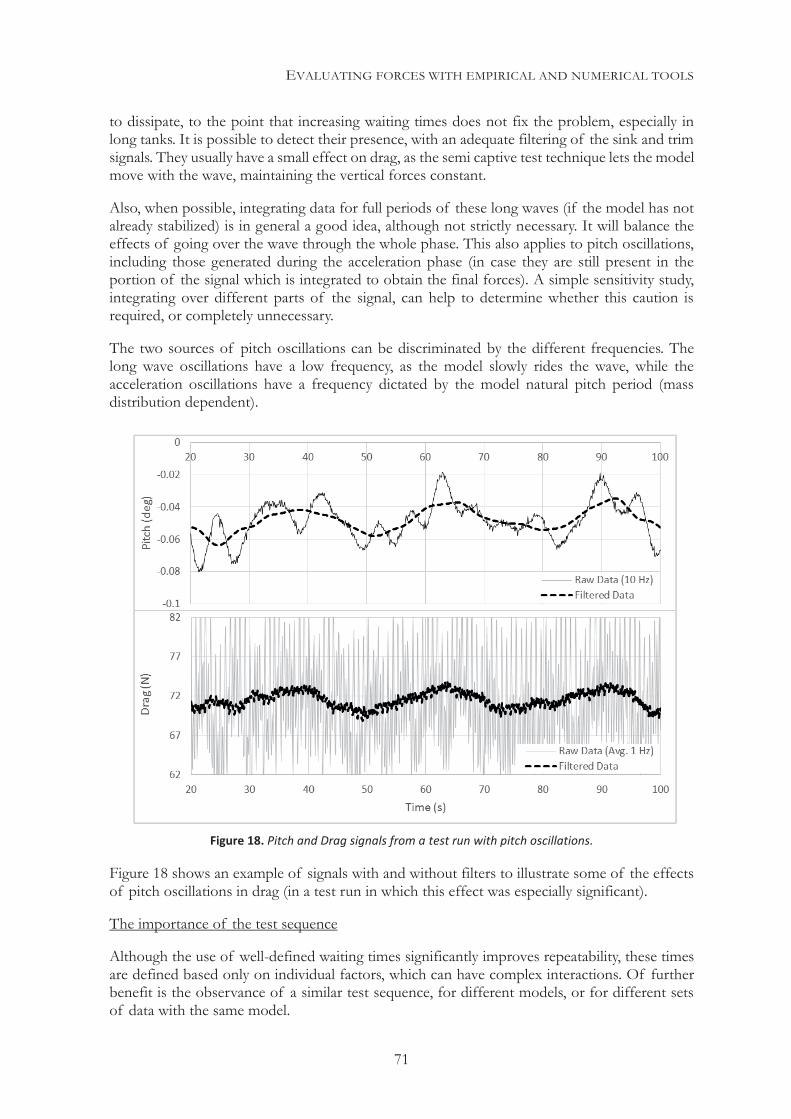
EVALUATING FORCES WITH EMPIRICAL AND NUMERICAL TOOLS
71
to dissipate, to the point that increasing waiting times does not fix the problem, especially in long tanks. It is possible to detect their presence, with an adequate filtering of the sink and trim signals. They usually have a small effect on drag, as the semi captive test technique lets the model move with the wave, maintaining the vertical forces constant.
Also, when possible, integrating data for full periods of these long waves (if the model has not already stabilized) is in general a good idea, although not strictly necessary. It will balance the effects of going over the wave through the whole phase. This also applies to pitch oscillations, including those generated during the acceleration phase (in case they are still present in the portion of the signal which is integrated to obtain the final forces). A simple sensitivity study, integrating over different parts of the signal, can help to determine whether this caution is required, or completely unnecessary.
The two sources of pitch oscillations can be discriminated by the different frequencies. The long wave oscillations have a low frequency, as the model slowly rides the wave, while the acceleration oscillations have a frequency dictated by the model natural pitch period (mass distribution dependent).
Figure 18 shows an example of signals with and without filters to illustrate some of the effects of pitch oscillations in drag (in a test run in which this effect was especially significant).
The importance of the test sequence
Although the use of well-defined waiting times significantly improves repeatability, these times are defined based only on individual factors, which can have complex interactions. Of further benefit is the observance of a similar test sequence, for different models, or for different sets of data with the same model.
Figure 18. Pitch and Drag signals from a test run with pitch oscillations.
EVALUATING FORCES WITH EMPIRICAL AND NUMERICAL TOOLS
72
The idea is to gradually increase the amount of energy put into the tank, and in parallel the measured forces. For instance, the amount of energy will increase with increasing speeds and also with increasing lift.
Based on this, a good strategy is to test points with increasing speeds for sets in which the generated lift will only depend on the speed. Then, a new set of data which generates more lift (for the same speeds) would be tested. This can mean increasing leeway when doing a leeway sweep (also with increasing speeds within the set). Sometimes, one or two low speed runs in between sets help to “recondition” the tank water.
This strategy serves two purposes: on one hand, any bias errors that may come from using “non-ideal” waiting times between runs will be consistent across different models, or even across different series with the same model (for other combinations of heel and leeway for instance). On the other hand, it maintains better proportionality of those errors, due to the energy left in the tank from the previous run, to the forces measured in the current run. This helps to preserve a more consistent level in the relative value of the errors relative to the forces.
On the other hand, it better maintains the proportionality of those errors, due to the energy left in the tank, to the forces measured. This helps to preserve a more consistent level in the relative value of the errors compared to the measured forces.
Running a low-speed and low-lift test point right after a high-speed and low-lift test point will certainly lead to bad results, and recorded time signals will show a relative variability significantly above average.
Within this test sequence criteria, a repeat test point run should whenever possible happen right after the questionable point (after the appropriate wait time), with the same test parameters. This requires constant real time analysis of the measured data, and using forces estimates, in order to determine within a few minutes whether the result of a run deviates enough from what it is expected to justify a repeat. When the doubts arise at a later stage, especially in cases with significant lift, it may be advisable to repeat at least a couple of the previous points, the way they would normally be tested in the normal sequence, as an intent to equalize as much as possible the water condition.
When a test point raises doubts, a check of the full load cell or processed forces signals over time can help to determine the reason for any anomalies, especially in the case of runs with lift (for which non-visible eddies may be present in the water). For instance, a shifting lift force signal through the run may reveal that the keel was going through some eddies, which may not have yet dissipated, suggesting that a longer waiting time may be required.
In some cases, because of this large-scale vorticity in the water, different parts of a keel may be subject to different incoming flow angles and speeds, in such a way that the global lift does not change much but the lift distribution does, altering the induced drag. A verification of the calculated effective span based on the measured lift and drag forces helps to detect such situation.
Problems of water temperature gradient with depth
One potential problem to which many tanks do not pay enough attention is the presence of a water temperature gradient with depth. It should be easy to measure the temperature both near the surface and in the more stable water near the bottom of the tank). The reason why this measurement at different depths is seldom performed is that in more conventional model testing
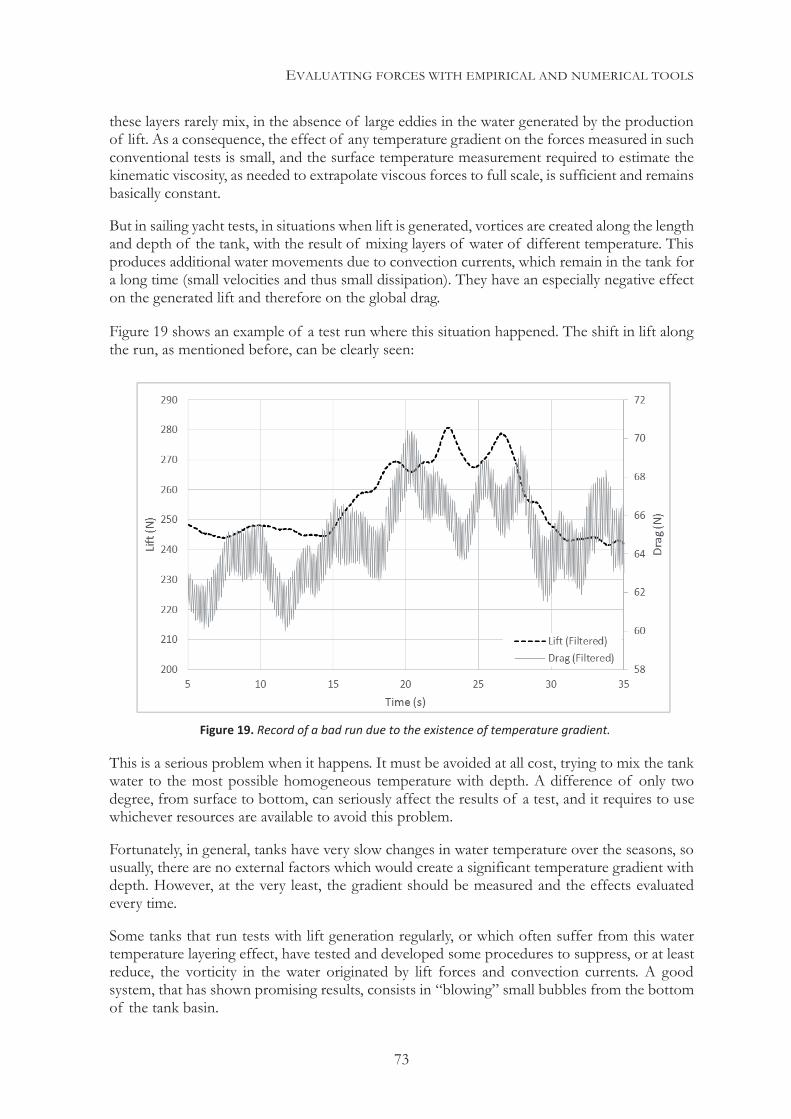
EVALUATING FORCES WITH EMPIRICAL AND NUMERICAL TOOLS
73
these layers rarely mix, in the absence of large eddies in the water generated by the production of lift. As a consequence, the effect of any temperature gradient on the forces measured in such conventional tests is small, and the surface temperature measurement required to estimate the kinematic viscosity, as needed to extrapolate viscous forces to full scale, is sufficient and remains basically constant.
But in sailing yacht tests, in situations when lift is generated, vortices are created along the length and depth of the tank, with the result of mixing layers of water of different temperature. This produces additional water movements due to convection currents, which remain in the tank for a long time (small velocities and thus small dissipation). They have an especially negative effect on the generated lift and therefore on the global drag.
Figure 19 shows an example of a test run where this situation happened. The shift in lift along the run, as mentioned before, can be clearly seen:
This is a serious problem when it happens. It must be avoided at all cost, trying to mix the tank water to the most possible homogeneous temperature with depth. A difference of only two degree, from surface to bottom, can seriously affect the results of a test, and it requires to use whichever resources are available to avoid this problem.
Fortunately, in general, tanks have very slow changes in water temperature over the seasons, so usually, there are no external factors which would create a significant temperature gradient with depth. However, at the very least, the gradient should be measured and the effects evaluated every time.
Some tanks that run tests with lift generation regularly, or which often suffer from this water temperature layering effect, have tested and developed some procedures to suppress, or at least reduce, the vorticity in the water originated by lift forces and convection currents. A good system, that has shown promising results, consists in “blowing” small bubbles from the bottom of the tank basin.
Figure 19. Record of a bad run due to the existence of temperature gradient.
EVALUATING FORCES WITH EMPIRICAL AND NUMERICAL TOOLS
74
This has two effects. The first effect is to mix the water making it more homogeneous from the temperature point of view. The second effect is to increase the speed at which the eddies are dissipated, breaking the larger and slower eddies into smaller and faster ones, and letting viscosity do the final work.
4.3.6 DIFFERENT MODELS AND TEST SESSIONS
With the exception of tests for a single model (and in this case the accuracy requirements are hardly as strict as when comparing different models), most tank programs are designed and planned to compare models. This accentuates the importance of consistency, which cannot be stressed enough.
Sometimes, these models are tested in the same “session” (understood as a group of tests, normally involving different models, that happen with no other interruptions than the normal test shifts) lasting several days or weeks, and in this case, it is easier to guarantee and control the consistency. But often, the tank test programs are longer and require a number of different tank sessions, spaced months or years apart and during different seasons. This means that the tank conditions may not be exactly the same, making comparisons an even more challenging exercise.
Every possible step must be taken to try and reproduce the exact conditions, but there is a limit on what can be done. In addition, calibrations may have changed, although repeating the same calibration procedures can guarantee a consistent measurement of the forces.
But despite these efforts, sometimes when high consistency is required, it is not uncommon to re-test a control model. Normally, a model from a previous session would be used as a way to provide a good assessment about the repeatability of the test. At the very least, this control model can provide information regarding any systematic bias, which can help to correct the results to make them consistent between sessions.
To do this, a small matrix is tested for the control model and results are compared to those of the previous session/s. This test matrix can be extended, should uncertainties arise.
In these situations, special cautions must be taken to guarantee that the model surface is kept with the same finish, but even more importantly, the control model geometry must be checked for stability. Storage, changes in temperature or humidity, etc. can alter the shape, in general with bending and torsion. It will be necessary to take corrective measures to restore the original shape, should that happen beyond an acceptable limit.
One comment must be made regarding the use of tests performed in different facilities, sometimes even at different scale.
This is not a common situation, except in the case of research, oriented to facilitate inter-facilities comparisons, or when building general analytical models with data from different sources (as it is the case of the IMS formulations for residuary drag). In this last situation, sometimes one specific set of tests in a given facility is intended to assess the effect of one parametric variation, which can then be ported to the general model. But also, it is common that the tested models become part of a bigger regression. In that case, it is a good practice to test a common control model, which will help to bridge post-processed results so that the general statistic base remains homogeneous.
EVALUATING FORCES WITH EMPIRICAL AND NUMERICAL TOOLS
75
This is a significant but necessary effort to obtain the best results, and in the absence of better information, no direct comparison should be made based on tank results from different facilities and/or model scales.
4.3.7 DATA EXPANSION TO FULL SCALE
Data expansion is a topic that has attracted a significant amount of research since the first model tests. A lot has been written about it and a reasonably good agreement has been reached in the scientific community regarding the procedures to use. Once again, we will refer here only to specific aspects related to the sailing yachts tests problem.
Given that the model speeds in a tank test are chosen so that the Froude number is the same as for the corresponding speeds in the full-scale yacht, the expansion of the so-called residuary drag and any other forces of potential nature (like lift or induced drag) scales up with the displacement.
As happens in virtually any other type of tank test, the viscous drag complicates things, mostly because of the following reasons:
Sailing yachts move in a range of heel angles, which change the shape of the immersed part of the hull.
The waves generated at medium to high speeds have an impact on the wetted surface and length, especially in the case of existence of shallow overhangs.
Appendages are distinctively separated elements with very different characteristic lengths, as compared to the hull and even between them.
Appendages may interfere with each other and sometimes they operate at high lift coefficients, making turbulence stimulation especially delicate, to avoid laminar separation that would not be present at full scale.
As a result of the above, experience has shown that the following precautions should be taken to guarantee a correct extrapolation of the viscous forces:
The ITTC 57 friction line with a calculated form factor is the usual approach for estimating the hull viscous drag, while some authors prefer the Shoenherr friction line. In absence of clear preferences, consistency again is key.
When expanding data for viscous drag generated by the hull, it is highly advisable to use dynamic lengths and wetted surfaces. This data may be measured from test photos (using as a reference a grid painted on the surface of the model), estimated as function of some parameters, or ideally, estimated by using some panel code with non-linear free surface calculation. This method can provide valuable estimates of the potential forces along with dynamic length and wetted surface data for the expansion, with a limited use of time and resources (certainly much less than when using a RANSE code).
Hull form factors should be determined without appendages attached to the canoe body. Given that the Reynolds numbers of the appendages for the required speeds are very low, the normal turbulence stimulation placed in them cannot always guarantee to force the transition. In addition, the difference in Reynolds numbers between hull and appendages would add an additional degree of uncertainty towards obtaining a global form factor.
EVALUATING FORCES WITH EMPIRICAL AND NUMERICAL TOOLS
76
Although some authors suggest the use of this technique, in the experience of this author the two methods produce different results with no clear trend.
In boats with low L/B and B/T ratios, the form factor may change with heel. In such cases, it is worth confirming the extent of change. Some formulas may be derived for corrections.
On the model, transition from laminar to turbulent flow is assumed to happen at the turbulence stimulation (or even earlier at high speeds if the values of the Reynolds number indicate so). At full scale, the Reynolds number along with an estimated turbulence level will allow to estimate where the transition is expected to happen. The appropriate friction coefficients should be used for the laminar and turbulent parts, along with estimated form factors. Form factors will normally depend on the thickness-to-chord ratios for lifting surfaces and on analogous parameters for bodies like bulbs. Several sources have proposed some variations of those form factors, but Hoerner (13) is a commonly used source.
The drag generated by the devices used for turbulence stimulation (not to be confused with the changes in the viscous drag because of their effect on the boundary layer transition) must be deducted from the total drag to expand.
In order to use the adequate form factors and friction coefficients for each element, appendages should be “stripped” from the hull and discriminated from each other, when estimating their viscous drag. For highly tapered keels, it is furthermore recommended to divide them span-wise into horizontal strips and use an accurate Reynolds number for each strip.
Interference drag is small for the model scale due to the limited thickness of the boundary layer at the intersection with appendages. However, it can be estimated and deducted. Then it will be calculated again and added for the full-scale boat with the appropriate parameters.
It is easy to see how some of the analytical models for the calculation of forces described in the previous Chapter come to use for estimating the viscous drag, that must be deducted at model scale to obtain the “pure” potential forces , then added again at full scale.
The final objective is to rebuild the full forces for the full-scale yacht, since those are the ones that will ultimately be used for the performance prediction. The data expansion process, like every step of tank testing, aims to obtain an accurate estimate of forces for the real yacht, but since assumptions and simplifications are made along the way, consistency is paramount when comparing different designs.
In their paper from 1990, DeBord and Teeters discuss in detail data expansion techniques, along with general test quality and accuracy (29).
4.3.8 A NOTE ON TESTS WITH FULLY-CAPTIVE MODELS
The semi-captive one described above is by far the most common type of test performed in a calm water tank. However, fully-captive tests are possible, in a way analogous to how numerical analyses can be performed at fixed sink and trim. Such tests are used for validation purposes or in specific cases when sink and trim equilibrium may be difficult to achieve with passive systems, like fully hydrofoil-supported boats.
One might think that captive tests would be a simpler method, but in fact with captive tests one faces new problems, that must be addressed.
EVALUATING FORCES WITH EMPIRICAL AND NUMERICAL TOOLS
77
One advantage of the semi-captive tests is that whatever the variation of the shape in the water surface, the boat will reach a vertical equilibrium only dependent on the hydrostatic and hydrodynamic vertical forces. Even if a long period longitudinal wave remains in the tank, most of the effects will be cancelled by this “natural” correction.
This is not the case for the fully-captive model, where the longitudinal wave will produce a variation even in the hydrostatic forces, as the hull goes through the different phases of it.
To make things worse, at higher speeds, the aerodynamic effects of the carriage itself produce a measurable alteration of the water surface, and thus an additional associated wave.
Therefore, when testing a captive model in situations where these effects may happen, it is recommended to:
Run tests with the model lifted out of the water (or without the model installed) and measure the resultant wave produced by the carriage at different speeds, in the location of the model.
Try to carry out the different runs at a consistent phase with the tank longitudinal wave.
Measure the tank wave height (independently of the local wave system created by the model), to determine its value at the location of the model at any point of the run. This way, corrections can be made for the variations in displacement created by the tank wave.
These points show that the idea of captive tests being a simpler technique is a misconception. Yet, the technique is useful in some situations, and then the previous recommendations should help to establish a starting point for setting procedures to improve their accuracy and consistency.
4.3.9 SEAKEEPING AND MANEUVERABILITY TESTS
These two kinds of tests are rarely used for sailing yacht performance prediction, given their complexity and the lack of full-scale data for validation. Also, they add the difficulty of requiring an adjustment of the model inertias so that the movements of the boat are properly scaled down (keeping in mind that time is scaled as well; therefore, motions are faster at model scale).
In addition, they require yaw movement ability, to enable the model to receive oblique waves, or to reproduce maneuvers. Such experiments are performed ideally in specifically equipped tanks, and for a sailing yacht this happens mostly for specific research purposes, which will not be discussed here.
However, a simple test in head waves conducted in a conventional tank equipped with a wave maker can give some idea about the drag added in waves. This is especially useful when dealing with frequencies of encounter which are far from the natural pitching one of the yacht, thus having little influence in its pitch motions. The result can be just an estimated added drag, which may for instance help to opt between two different bow shapes producing the same flat-water performance.
Similarly, some automated yaw sweep while running at a given speed can provide an indication of steering drag.
EVALUATING FORCES WITH EMPIRICAL AND NUMERICAL TOOLS
78
In both cases, the only “routine” tests performed at times are intended to provide a basic assessment of the increase in drag that can be expected. This can be used to correct the estimated resistance added in waves in the VPP, rather than provide an accurate description of these phenomena.
WIND TUNNEL TESTS The wind tunnel tests are the other important experimental tool for estimating the forces in a sailing yacht. The experiments are performed in a dedicated facility.
There are different types of wind tunnels, some working in a closed circuit where the test chamber is a closed section of the tunnel, and some working in an open circuit where the test chamber is open to the atmosphere from which the air is taken and to which it is returned. Closed circuit wind tunnels allow higher speeds and larger models to be tested.
Most facilities used for sailing yacht testing use a closed circuit and chamber, providing a highly controlled environment. However, wind tunnels with an open test chamber (and sometimes without any air recirculation), blowing air at lower speeds are a much cheaper alternative, often available to universities, and when used properly they can provide valuable results.
Beside these configurations, there exist a number of wind tunnels with specific features, ranging from supersonic tests to cryogenic environments. Their purpose is varied and can include studies with cars, airplanes, trains, buildings, smoke, noise and others.
In all the cases of interest here, a test chamber receives air moving at a certain velocity, usually from a recirculating system. The moving air is conditioned before the test area by different types of grids and/or deflectors. These are intended to provide a specific level of turbulence and/or a change of the incoming flow direction or velocity for different areas of the chamber. This permits for instance, to reproduce at the test scale the wind gradient over the surface of the water.
Mounted on one or more of the walls of the wind tunnel (normally the floor or ceiling) are dynamometer/attachment systems for the test models (in most cases the dynamometer provides the support for the model). The system allows some controlled movements, in order to make changes to the testing position. This is not too different from the tank arrangement, except that in this case tests are normally performed with a fully-captive model. The changes in position are purely for adjusting the test parameters.
The dynamometer (also called balance in wind tunnels) is normally a six component unit placed in a “hidden” position so that only the models to be tested are exposed to the effect of the moving air (wind).
As is the case with models used in the tank, the wind tunnel models are normally built at a reduced scale; thus, scale effects have to be taken into consideration. Regarding the fluid (air) properties and model size, two factors need to be considered: the Mach number, which relates the inertial forces and the compressibility of the fluid (and it is defined as the ratio between the air speed and the speed of sound), and the already defined Reynolds number, which relates the inertial forces and the frictional forces.
In the normal use of wind tunnels for sailing yachts, the range of air speeds at which tests are performed permits to safely ignore the compressibility of the air. This leaves the Reynolds
EVALUATING FORCES WITH EMPIRICAL AND NUMERICAL TOOLS
79
number as the main factor. Ideally, it must match the Reynolds number of the full-scale situation, or if that is not possible, corrections should be considered.
In any of these cases, the use of wind tunnel tests as part of a performance prediction process has been less widespread than the use of tank tests up until today. The most common application for wind tunnel results has been to generate analytical sail models. A significant effort is involved in treating and correlating the measured data to obtain those sail models.
We will discuss briefly the potential use of wind tunnel tests in direct performance predictions, evaluating appendages or aerodynamic forces, and some precautions to be taken.
4.4.1 WIND TUNNEL TESTS FOR APPENDAGES EVALUATION
The wind tunnel has been used in ambitious performance prediction programs for appendage evaluation when the effect of the free surface is not significant. This may happen either because there is no strong interaction with the free surface, or because the parameters to analyze are not closely related to its presence, with the variations on the forces being more important than their absolute values.
This is for example the case of complex keels with bulbs and winglets, where on top of measuring the potential lift/drag generated, it is important to have the ability to test at the same Reynolds number or close. This becomes important for evaluating viscous phenomena like the extent of a laminar boundary layer and its influence on drag.
The relatively high speeds at which most wind tunnels can operate provide the factor required to compensate for the differences in kinematic viscosity between air and water, in order to match the Reynolds number of the normal sailing conditions. In the case of appendages, the model scale is usually close to one, and sometimes, in large facilities, even greater than one. This scale helps to achieve similar values of Reynolds numbers to those encountered at full scale, as desired.
Additionally, the wind tunnel has the advantage over the towing tank that it can provide flow visualization tools, as well as a faster way to test a dense matrix of data once the model is installed in the dynamometer.
It is common to attach the appendages to the dynamometer through a hull dummy (or even a hull + deformed free surface), to better simulate the flow and interaction between the different components.
The calibration, model accuracy and quality requirements are analogous to those of the tank, with the exception of turbulence stimulation, normally not needed given that the correct Reynolds number is represented.
However, because of the high cost of the models, due to their size and the structural and surface finish requirements, and because of the improvements in the numerical codes (especially with fully attached flows), this type of tests is becoming unusual. Nowadays, they are only performed in some rare well-funded programs, and most of the times for validation purposes.
Moreover, an additional complication with wind tunnel data is that forces not captured by the experiment must be added to complete the full set of hydrodynamic forces (such as the different
EVALUATING FORCES WITH EMPIRICAL AND NUMERICAL TOOLS
80
components of the drag generated by the hull), as well as the effects of any interactions with the free surface if they are considered significant.
4.4.2 WIND TUNNEL TESTS FOR AERODYNAMIC FORCES
The main area in which the wind tunnel is used is in estimating the aerodynamic lift and drag generated by the sail plan and the hull/deck, or cross structure in the case of multihulls. These elements can be tested separately or together to better account for the mutual interactions, which can also be the objective of the tests, as it happens with end plating studies.
As mentioned before, the most advanced facilities allow establishing a scaled down wind gradient in the location of the sailplan scale model. The sailplan model allows adjustment of chosen sail trim parameters, and can be rotated to change the wind angle, and sometimes heel angle.
It is not uncommon for the process to be automated and even linked to a VPP. This is done, in some cases, to assess whether the sail trim for which the forces are measured corresponds to the optimum solution.
This is a good approach when trying to make a real time interpretation of the result, given that the driving force may not be sufficient for drawing a conclusion for two main reasons: a larger side force generated along with the driving force will create more hydrodynamic induced drag; also, different span-wise lift distributions will affect the heel moment generated by the sail plan. Use of a VPP is necessary to balance those effects and determine the optimum trim. Le Pelley and Richards discuss an example of this process in their paper presented at the 20th CSYS (31).
Another approach is to test a range of trim parameters and record the forces generated, in order to create a more complete multi-parametric sail model based on the experimental data. This is obviously more time consuming, both testing and certainly post-processing the data, but it provides a much more complete result, to use in a more detailed calculation environment. The final adjustment of the sail trim parameters is left again to the VPP, but based this time on the whole recorded data set.
Again, the aim is to test at the same Reynolds number as the full-scale one, or close, in order to facilitate the expansion of the results by avoiding as much as possible qualitative differences in the nature of the flow and boundary layer (such as separation). However, a number of factors can impede the achievement of this condition, such as the maximum speed capacity of the wind tunnel, or the scale of the forces generated, or structural limitations. As P. Hawkins shows in his master thesis (32), this does not invalidate the usefulness of tests that are run at lower speeds, as it is often the case.
F. Fossati et al. make in their paper (30) presented in the 2006 HPYD conference in Auckland (NZ) an interesting review of the wind tunnel techniques for the optimization of sailing yachts aerodynamics.
Some considerations regarding the construction of scaled down sail for tests
When testing sails, due to the nature of their construction, a number of other factors are influenced by the scale relative to the air speed. P. Izaguirre provides in her PhD thesis (33) the following clear and descriptive list:
EVALUATING FORCES WITH EMPIRICAL AND NUMERICAL TOOLS
81
Membrane mass ratio. This ratio is related to inertial forces. Since wind tunnel tests are conducted under static loads, this ratio is not important. It is only taken into account when dynamic effects are considered.
Membrane elasticity ratio. It describes the aero-elastic effects of the sailcloth. For most testing conditions sail stretch is small. A membrane elasticity ratio comparable to full scale can be achieved by selecting the material properties of the model sail to reflect the changes in flow speed between the wind tunnel and full-scale.
Membrane fold height ratio. It provides an estimation of the sailcloth stiffness. The material of the sailcloth of the model should permit the sail to adopt the scaled flying shape. The fold height ratio does not need to be matched exactly to the full-scale sail if the model sail is flexible enough to achieve its natural shape.
Weight/pressure ratio. It relates the gravitational force to the pressure loading on the sail. It has been demonstrated that, as long as it is within certain values, it does not need to be matched.
These important factors must be considered, in addition to taking special care in the construction of the model mast and rig, given their effect on the sails. Keeping the above factors as close as possible to reality will certainly be desirable, and it will help to improve the accuracy of the test through a range of wind speeds and generated forces.
This is verified by trying to match the actual flying shapes (and even measuring that shape when possible). This becomes a significant challenge.
However, as it has been suggested before, in some tests the main purpose is the comparison of different design alternatives. In those cases, maintaining consistency between the above mentioned factors for the different tests will be even more important than how close they are to the full-scale situation.
Sail Trim
Depending on the final objective of the tests, the sails may need to be adjustable as close as possible to how it is done in reality. Adjustments are often performed during the test by experienced sail trimmers in order to guarantee this consistency.
The forces are measured and recorded continuously while adjustments are made to attain the desired close-to-optimum trim of the sails. This optimum may intend to maximize the driving force for a heel moment that is constant or not.
Or the optimum sought may be a performance optimum, which can be assessed when the test is performed with a VPP using in real time the measured sail forces to calculate an equilibrium situation. This situation has become more common nowadays, depending on the final objective of the experiment.
Sometimes, automated trim variations are tested in order to provide a dense database to separately assess the effect of different adjustments.
Given the nature of the wind tunnel (where unlike in the tank, no waiting times are required), with the proper setup this is an easy task, and most of the effort is on the work performed on the acquired data.
EVALUATING FORCES WITH EMPIRICAL AND NUMERICAL TOOLS
82
Data from wind tunnel sail tests.
Different aerodynamic tests can be performed in the wind tunnel, and as stated before, they may involve from just a simple sail plan to a full configuration above the waterline. This will depend on the purpose of the experiment and which factors are being analyzed.
However, there is a basic set of data of interest. It will be constituted of the data necessary to evaluate forces, at least for one wind speed, over a range of apparent wind angles in which the yacht will normally sail. The final outcome will be a set of lift and drag coefficients (along with moments or centers of effort) vs. apparent wind angles for a full-scale situation. This usually involves the use of corrections and extrapolation techniques to account for the effects of scale.
Heel effects can either be estimated with mathematical models deduced from theory, or as part of the experiment itself. The importance of this will, again, depend on the nature of the elements being tested.
Beyond that, the remaining independent parameters will be either different sail sizes and/or geometries and trim parameters. Trim parameters can affect the shape of the sails, changing mainly camber and twist but not only. They play an important role on the sail plan efficiency, and they also become a key adjustment parameter for the VPP, as they provide depowering handles that are optimized when analyzing performance. Should these parametric changes not be part of the wind tunnel tests, the sail coefficients obtained from the tests can be assumed to correspond to a maximum driving force (or close), and the final depowering can be implemented in the sail model.
Wind tunnel experiments with sails in general
Beyond the most traditional use of the wind tunnel as a way to obtain sail coefficients, the number of experiments intended for validation have increased with the capabilities of the numerical methods, especially when dealing with viscous phenomena. The intention is to rely more and more on the numerical tools for the generation of sail coefficients, in routine studies providing support for the sail designers.
The test setups, procedures and the process of obtaining the aerodynamic forces are similar for most wind tunnel experiments with sails. They are well described in some detailed published papers, that also discuss the post-processing of the collected data and the design of analytical models based on them.
However, unlike the case of hydrodynamic tests, this is not a common task in which the results are directly used to feed a VPP (for performance prediction), but rather the beginning of complex studies which are normally performed by the scientist in charge of the experiment. The level of detail of these studies is considered to be beyond the scope of this research.
It is important to note that a significant amount of effort has been put over time, including in the last few years, in the use of the wind tunnel to provide a very complete base of information for the sail models that are incorporated in the IMS VPP. The models currently implemented are based mainly on the tests performed at the Politecnico di Milano under the supervision of F. Fossati (10). These are probably the most complete and detailed general purpose sail models used in velocity prediction programs, and their use has transcended the (strict) application to the IMS, as they are implemented in a wide range of performance prediction tools used all over the world.
EVALUATING FORCES WITH EMPIRICAL AND NUMERICAL TOOLS
83
GENERATION OF NUMERICAL DATA Since the late 1970’s, Computational Fluid Dynamics have played an increasing role in the calculation of hydro and aerodynamic forces throughout the use of a range of evolving methods.
The basic idea is to solve the Navier-Stokes equations by means of discretization, making as few simplifications as possible as they may compromise the result. Different methods have been experimented and used, but with the dramatic increase in computational power over the last two decades, a door has been opened to improve the accuracy and reliability of such methods.
Another consequence of this progress has been to put closer to the hands of the designers and performance analysts a tool which is turning into the main source of data, not only to create and tune analytical models but to directly feed specialized VPPs.
Different alternatives provide different solutions with different requirements in terms of resources, time and required expertise. In this section, we will discuss the potential uses and precautions associated with them and propose some strategies for obtaining data.
4.5.1 TYPES OF CODES
Describing, even briefly, the nature and characteristics of numerical codes themselves can be a never-ending endeavor. For this reason, at this point the discussion will be limited to the most basic aspects related to those codes that can calculate forces in a sailing yacht with a reasonable amount of resources.
Lifting line
Presented independently by Frederick W. Lanchester in 1907 (34), and by Ludwig Prandtl in 1918–1919 (14), the lifting-line theory consists in a mathematical model for the prediction of the span load of a 3D wing or appendage and its induced drag.
The initial theory considered that the lift is located on a straight single bound vortex (normally positioned on the quarter-chord line of the planform), which is called lifting-line, with a vortex-wake streaming straight back from it. Applying the Kutta-Joukowski theorem, the bound vortex strength is then connected to the lift per span unit. And according to Helmholtz’s second theorem, when the lift changes along the span, the related variation in bound vortex strength is transferred into the wake. If a straight lifting line is assumed, only the trailing vortex wake, evaluated in the lifting line, has an influence in downwash.
But the lifting line itself, generally, is not straight. In this case, the bound vortex has an effect on the downwash and that has to be considered. However, if this effect is evaluated on the lifting line itself, the theory does not work anymore (a curved lifting line has an infinite self-induced velocity). One of the solutions is to evaluate the downwash effect on a line located aft of the lifting line (at the 3/4-chord location).
In 1964, Van Dyke (35) conducted some work to justify that this theory could be considered a valid approximation for high aspect ratio lifting surfaces with small loading conditions.
EVALUATING FORCES WITH EMPIRICAL AND NUMERICAL TOOLS
84
Vortex Lattice
In order to overcome the limitation of the lifting line theory, namely limited to straight elements with moderate to high aspect ratio, a more sophisticated model was developed. Extending the Prantdl formulation, the so-called lifting surface model consists in placing a number of lifting lines along the element (wing or appendage) in the direction of its chord. In fact, if an infinite number of these lines are considered, it results in a vortex sheet. In addition, a system of trailing vortices is associated to each of these lifting lines. This system crosses the whole element in a direction perpendicular to the lifting lines and continues into the wake. Once the lifting surface is defined, the objective is to obtain the induced velocity over the lifting element.
With the increase of computational power, a numerical solving technique has arisen. If the lifting surface is discretized through a number of panels with a horseshoe vortex and a control point into each panel, the entire element is covered by a lattice of vortices with unknown strength. When applying the flow-tangency condition and the Biot-Savart Law to the control points, an algebraic equation system appears (36). This system can be solved for the vortices unknown strengths. This numerical approach is called the Vortex Lattice method.
Panel codes
For the resolution of non-viscous problems (as is the case with the methods described above), another strategy is possible. This approach is based on the assumption that in absence of viscosity, the flow velocity derives from a scalar potential. Then the continuity equation transforms into a Laplace equation for the velocity potential. This potential can be described as the sum of the ones corresponding to an external uniform flow and to a body perturbation flow (superposition principle for linear equations). After applying some boundary conditions to the flow, the problem consists in finding a perturbation body flow potential that satisfies the Laplace equation and the boundary conditions. This potential can be described as a group of elementary singularities distributed over the contours of the body. This is the reason why the body surface can be discretized as a distribution of panels that incorporate those singularities.
One important feature of this method is the possibility to solve problems involving a free surface, with generation of waves. This can be achieved with a free surface panelization with special boundary conditions. One of the main difficulties is to overcome the non-linear effects over the free surface. Over the years, this method has evolved from solving a velocity field for a fixed flat free surface, to a linearization scheme of the free surface for the boundary condition (Dawson method (37)), then to more complex non-linear schemes, like the one presented in Hoyte C. Raven´s PhD thesis (38).
Even if this method allows solving ship wave resistance problems, it presents some disadvantages. Sometimes, a lifting surface close to the free surface or an immerse transom can create local peaks of pressure. To solve this kind of problems, specific panelizations and boundary conditions have to be used in the specific zones where these conditions appear.
For a simple calculation of the viscous forces, this type of codes can be coupled (in a weak or strong matter) with specific boundary layer codes.
Euler codes
This method corresponds to the solution of the Euler Equations, which are a simplification of the Navier-Stokes equations. The simplification consists in eliminating the viscous and heat-conduction terms of the equations. For this reason, this method is suitable for non-viscous
EVALUATING FORCES WITH EMPIRICAL AND NUMERICAL TOOLS
85
flows with or without vorticity. One of the main advantages, in comparison to the Potential Panel Method, is that this kind of code it is capable of capturing discontinuities, like shock waves. These kinds of discontinuities are very useful when a supersonic flow is studied, but this is outside of our area of interest. This compounded with the fact that such code is more computationally demanding than potential codes explains why it is not commonly used for solving the kind of problems discussed here.
RANSE codes
When there is a need to work with viscous flows, like in the calculation of the full hydrodynamic resistance of a hull, the full Navier-Stokes equations have to be solved. A Direct Numerical Simulation (where all turbulence scales are solved) is very computationally demanding and limited at this moment to solving simple flow geometries problems. The solution is to use a Reynolds-Averaged form of the Navier-Stokes equations (RANSE), with a model of turbulence (to avoid the need to solve all turbulence scales directly). The most convenient turbulence model for hydrodynamic naval applications is the SST K-Omega model, but for other applications, other models are available, like for example the K-Epsilon or Spalart-Allmaras turbulence models for aerodynamic problems.
This type of codes, called RANSE codes, can be used to solve steady or unsteady problems. The Unsteady Reynolds-Averaged Navier-Stokes (URANS) codes can be used, for instance, to simulate the towing tank tests with sink and trim. Even if this kind of simulations could be considered quasi-steady, the fact is that the codes available at the moment can only solve free-surface problems with URANS. This implies the need of more computational resources than the steady RANSE solvers.
Instead of using only panels on the free surface and the body surface (like in the Potential Panel Method), this method discretizes the whole computational fluid domain with a mesh, normally based on finite element or finite volume schemes. This mesh can be structured or unstructured, and can use different types of elements, such as tetrahedral, hexahedral or polyhedral. Usually, a towing-tank-like test simulation uses hexahedral meshes because of the flow problem alignment with the mesh and the better convergence of the solver. Special meshing models are used for modeling the boundary layer near body surfaces, like prism layer meshing where “wall functions” are applied.
To model the free surface, a specific model must be used, like for example the Volume of Fluid model (VOF) with a high-resolution advection scheme such as HRIC (High Resolution Interface Capturing scheme).
If some dynamic movement needs to be taken into account, different techniques could be used. For instance, moving the whole mesh considering the free surface situation (like in the original dynamic fluid-body interaction (DFBI) model implemented in Star-CCM+ (39)). Another solution to the problem, commonly used nowadays, is the overset grid technique in which one mesh moves over another general one. This is also called the Chimera technique, as that was the name of it first implementation, developed by NASA in the mid 80’s (40) (41).
4.5.2 SOME PRECAUTIONS ON THE USE OF DIFFERENT CODES
A number of aspects common to the different numerical tools are discussed before going to specific uses.
EVALUATING FORCES WITH EMPIRICAL AND NUMERICAL TOOLS
86
The first one is related to the fact that, while accuracy in the quantitative calculation of the actual forces has improved, the numerical tools are particularly well suited for comparison purposes. This does not mean that they cannot calculate absolute values accurately, but in that case a significant validation effort is necessary. However, they are very good at detecting the impact on the forces of reasonably small parametric changes in the geometry or the conditions.
Obviously, the need for validation depends on the experience of the person running one specific code, and on how well that code and the setup of the simulation perform with the specific type of problem being analyzed. Confidence in the simulation relies on a good physical understanding of the problem, and on past experience, in which a validation process was involved at some point, in most cases against experimental results collected with that specific purpose.
Consistency
Consistency is again paramount, to the point of deserving a specific discussion. Unless a sensitivity analysis shows otherwise, factors such as the running parameters, code settings, wall laws, turbulence models or boundary conditions should remain constant between the different runs for a single model or for different models.
The same principle applies to the generated discretizations, which should be of similar densities (relative densities) and topologies. Differences should be questioned, unless sensitivities studies show otherwise.
Sometimes, specific effects are evaluated that require specific settings. For instance, a correct evaluation of the effects from an immersed transom at different speeds will require specific meshes and boundary conditions, different from those used to analyze the general model where this phenomena is not present.
But in general, topological similarity provides a first step towards consistency. Most tools provide this, maintaining the meshing limitations relative to the geometry variations constant (like cluster to curvature criteria, elements proportions, density changes rate, type of elements and boundary conditions variations, etc.).
When specific problems require specific settings that alter some aspect of the desired consistency (such as a topologically different mesh for capturing the local effects of an immersed transom), comparisons can still be performed. However, special care must be taken to translate the effects on forces calculated this way into the general models (intended to perform a generic calculation), so that they can be compared with other designs or different conditions (which may not include the phenomena that required those settings). This way, it will be possible to confirm that the final differences are not created by numerical inconsistencies rather than by the physical effects themselves.
Code limitations.
When running numerical tools in order to obtain forces, one common problem comes from ignoring their limitations, given that they will still produce results even if outside the limits of the codes, results which, while reasonable in appearance (this is the danger), are not correct.
An example is the analysis performed by a panel code with a linear treatment of free surface in a hull with long shallow overhangs. The overhangs will be ignored by the code after deforming the free surface according to the calculated pressure map, but they will have a very significant
EVALUATING FORCES WITH EMPIRICAL AND NUMERICAL TOOLS
87
effect on the final dynamic length, wetted surface and, thus, drag. Still, results will be obtained, and a performance prediction based on those will lead to the wrong conclusions.
Therefore, it is important to have a sufficient level of awareness regarding the correct use of the different codes, including their strengths and limitations. This allows, for instance, to use simpler codes for specific tasks, which at times even provide a more accurate result, not influenced by aspects that can add extra numerical uncertainty with more complex codes.
Another simple example of limitation, this time driven more by a knowledge of the physics involved than knowledge of the code itself, is when a basic lifting line method is used to estimate the ideal lift distribution, of a sail plan for instance. The optimum result, considering both the lift/induced drag forces and their effect on the generated roll moment, may include sections with airfoils not able to achieve the required lift coefficients. This can be the case of lift coefficients which are too high or maybe negative, both impossible for a conventional sail, but which might be possible for a wing sail.
In these cases, judgement must be applied as to whether the results are achievable or if some constraints should be imposed to the calculations. These examples are not intended to point out advantages or disadvantages of specific codes (this will briefly discussed later). They just illustrate ways in which the code limitations can give rise to misleading answers.
Use with data from more or less accurate origin
Although this will be discussed in more detail in the next Chapter, it is necessary to make here a mention regarding how some numerical results may fit with data from a different origin.
When talking about code limitations, it has been described how a more basic code, simpler and faster to run, may help to fill the parametric space. These results can then be corrected using a limited set of data produced by a more accurate code, using a short matrix designed for this purpose.
This is a common scenario. However, there may be other situations, in which the calculation of the forces is based on analytical models, but where some numerical results provide insight into the influence of changes in one specific parameter onto those forces. In that case, those limited numerical calculations can significantly improve the accuracy of the prediction, still based mostly on generalist analytical models.
A good example of this is when evaluating planform shape for a curved board with variable chord lengths. In this situation, calculating the effective span to be used in the rest of the analytical calculations with something as simple as a lifting-line analysis, can provide a much more accurate result than just estimating it from the physical span and average chord.
Computational requirements
It is not uncommon to have access to codes that can potentially run extremely ambitious problems in terms of size, with tens of millions of elements. It is tempting to seek better accuracy by using a dense discretization. This has an obvious impact on the computational requirements and the execution times (as well as convergence).
This dense discretization may provide better accuracy, but not necessarily, and it may compromise convergence.
EVALUATING FORCES WITH EMPIRICAL AND NUMERICAL TOOLS
88
More importantly, before planning a program to obtain numerical results, it is necessary to define the available resources (mainly the timeframe) and balance a number of factors like:
Mesh density and size (accuracy) vs. A denser matrix of test points.
Mesh density and size vs. Number of parametric variations to evaluate.
Determine whether different parts of the problem require a more detailed discretization than others.
Determine whether a denser discretization have an impact on convergence beyond the size implications.
Again, some simple sensitivity studies will answer some of the questions regarding the adequate densities to be used, studies that sometimes can be replaced by experience.
It is also important to consider the use of more than one code. Sometimes, a faster code can help to populate a denser matrix (it may be able to evaluate accurately some of the parameter changes) and a more time consuming code can provide corrections to make the final results more accurate.
4.5.3 USES OF THE DIFFERENT CODES
Beyond the description of the fundamentals of the different types of codes, there are specific uses, which have become common and are part of the design and performance prediction toolbox, and they have been evolving over the last 30 years. These uses will be discussed in some detail below, with specific recommendations for their application.
Lifting-line codes.
They are the simplest choice for numerical analysis, and are still used for specific tasks. Those tasks are, in general, related to optimization studies that aim to find optimal span-wise lift distributions in simple geometries, always within the limitations of the lifting-line theory.
As was described before, this type of code provides, for a given distribution of lift along the span, a resultant lift, induced drag, and the effective angles of attack along the span. For a given geometry, the lift per unit span will be conditioned by the local transverse sections and effective angles of attack (affected by the downwash, as mentioned in the description of the code). The local lift characteristics can be either obtained from the bi-dimensional foil sections published data, or calculated with numerical tools like Xfoil (42) or the Eppler (43) code.
This allows building a global set of forces from a relatively simple calculation. However, in order to obtain the total drag, it will be necessary to estimate the viscous component, based to the body geometry and the velocities field around it. This limitation applies to any potential code.
Also, it is important to evaluate with these codes only parametric variations of which the codes can capture the effects. For instance, a number of lifting-line codes cannot deal with the effects of sweepback in geometries, but they still provide a result (incorrect regarding that sweepback variation). So here again, one must be cautious to take into account the limits of what a code can provide.
EVALUATING FORCES WITH EMPIRICAL AND NUMERICAL TOOLS
89
The accuracy of a lifting-line code is reasonable, and it may be a good alternative to populate a dense matrix (given the fact that lifting-line codes provide an extremely fast calculation), to which corrections can then be applied, based on a limited set of specific points calculated with more accurate and more time consuming codes.
This works well with hydrodynamic lifting surfaces that have their top end fully end-plated and their tip free. In the case of surface piercing foils, assuming a free tip at the piercing point also provides a close enough approximation.
Sail plan forces and target lift distributions are also areas where these codes are a good source of initial or even general estimates (with the cautions made before, regarding achievable lift coefficients).
Lifting-line codes are used regularly to explore what the desired lift distribution may be. That knowledge can then be used to design the geometry, using that distribution as a target. After that, the geometries can be analyzed with more sophisticated numerical tools.
As an example of this, even today lifting-line codes are sometimes used to look for initial target lift distributions in the curved boards used in the America’s Cup foiling catamarans; VPP calculations are run based on the estimated differences in forces and the results are used to determine the operating conditions for which the foil cross-sections must be designed.
Vortex Lattice codes.
Vortex lattice codes are historically amongst the first codes used in yacht design when working with appendages and sails, and while they are still sometimes used for keels, their use for hydrodynamic calculations has severely declined in favor of panel or RANS codes.
However, they are still successfully used for sails with attached flow, as is the case for upwind sailing or for high-speed sailing, as the apparent wind angles remain small enough to guarantee minimal separation.
These codes, used mostly by sail designers, have evolved from a tool that purely estimates forces or calculates sail coefficients for the VPPs, to a tool coupled with VPPs to directly evaluate the impact of design or trim changes in a more realistic way. This also provides an immediate assessment of the efficiency of the sail design or trim setting by directly estimating the impact on the final performance.
There have been a few options amongst these codes for sails, like SK2V from the Massachusetts Institute of Technology (MIT), but Flow, a proprietary code from North Sails ©, is probably the most used by sail designers nowadays.
Flow is a vortex lattice code coupled with the structural code Membrain, which allows iterating between them to make calculations based on the actual flying shapes of the sails. The structural properties of the sails (calculated as a membrane, with its properties built from its own structure, layer to layer) are taken into consideration along with the mast and rigging to progressively deform the sail plan until a convergence is achieved for a given sail trim. The forces and actual flying shape are the result.
The sail trim reproduces the actual trimming procedures on board the real yacht for a realistic handling of the sail shape, permitting to adjust the mainsheet tension, traveler position, cunningham tension, and even to adjust the rigging to control the mast.
EVALUATING FORCES WITH EMPIRICAL AND NUMERICAL TOOLS
90
An estimate of the viscous drag by means of a two dimensional boundary layer calculation completes the relevant forces.
Although Flow has been available since the 90’s, a version of this code has been developed since 2011 to allow the same calculations for wing sails, with their own peculiarities and adapted trim parameters, and it made its debut during the 34th America’s Cup campaign.
Panel Codes.
Vortex lattice codes are more suited than panel codes to calculate forces on sails, which have almost zero thickness. However, for wing sails, increasingly popular, panel codes are becoming a good alternative. Actually, the version of “Flow” intended to calculate wing sails uses a panel method to calculate the potential forces. It still reproduces faithfully the normal sailing controls, and works coupled with the structural equivalent to Membrain”.
But panel codes are used today in sailing yacht design mainly to calculate hydrodynamic forces generated by hulls and appendages, in most cases including the calculation of the free surface.
Even in the case of analyses performed with a detailed discretization (surface meshes), the execution times permit the calculation of a dense matrix of points from one day to the next, making it very attractive for calculations in which results are required in a short time. But convergence is affected when the number of panels grows beyond a certain point, which sets practical limits.
Needless to say, these codes work well only when no separation phenomena occur, which is not a very limiting condition for the generally slender sailing yachts in normal conditions.
A number of codes have been used in the past with appendages and a fixed free surface, providing a good estimate of lift and induced drag. Sometimes they have been run with coupled boundary layer codes, which allow a good estimate of the viscous forces, permitting to assess laminar-turbulent transitions. Normally, this is done with a weakly coupled boundary layer analysis, which permits to obtain a good estimate of the viscous forces when no significant thickness increase of the boundary layer is expected.
However, at times the boundary layer codes are executed with a strong coupling, meaning that the potential calculations will then be run on a geometry modified by the boundary layer thickness. This will be repeated iteratively until convergence is achieved.
When the main target of the analysis is the hull residuary drag, it is necessary to consider a non-fixed free surface subject to the effect of the pressure field. For reasons explained before (related to the effects of the overhangs), given the change in the waterline and wetted surface in sailing yachts with speed, the use of a non-linear treatment of the free surface is necessary in most cases. Simply calculating a deformed free surface based on the pressure field resulting from the first converged solution would provide just a first step to recalculate the waterline and its hydrostatic effects, but little more. Additional iterations are required to adjust the free surface shape under the influence of the hull moving through the water.
This is especially significant when the panel code is run in a similar way to the towing tank experiments, providing a displacement and center of gravity and leaving the sink and trim free, while corrections are provided for the estimated forces of the sail plan to drive the yacht for each condition. In this case, a full hydrostatic calculation needs to be performed after each
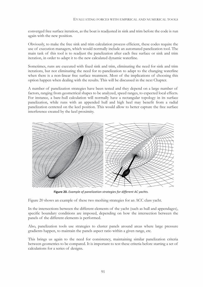
EVALUATING FORCES WITH EMPIRICAL AND NUMERICAL TOOLS
91
converged free surface iteration, as the boat is readjusted in sink and trim before the code is run again with the new position.
Obviously, to make the free sink and trim calculation process efficient, these codes require the use of execution managers, which would normally include an automated panelization tool. The main task of this tool is to readjust the panelization after each free surface or sink and trim iteration, in order to adapt it to the new calculated dynamic waterline.
Sometimes, runs are executed with fixed sink and trim, eliminating the need for sink and trim iterations, but not eliminating the need for re-panelization to adapt to the changing waterline when there is a non-linear free surface treatment. Most of the implications of choosing this option happen when dealing with the results. This will be discussed in the next Chapter.
A number of panelization strategies have been tested and they depend on a large number of factors, ranging from geometrical shapes to be analyzed, speed ranges, to expected local effects. For instance, a bare-hull calculation will normally have a rectangular topology in its surface panelization, while runs with an appended hull and high heel may benefit from a radial panelization centered on the keel position. This would allow to better capture the free surface interference created by the keel proximity.
Figure 20 shows an example of these two meshing strategies for an ACC class yacht.
In the intersections between the different elements of the yacht (such as hull and appendages), specific boundary conditions are imposed, depending on how the intersection between the panels of the different elements is performed.
Also, panelization tools use strategies to cluster panels around areas where large pressure gradients happen, to maintain the panels aspect ratio within a given range, etc.
This brings us again to the need for consistency, maintaining similar panelization criteria between geometries to be compared. It is important to test these criteria before starting a set of calculations for a series of designs.
Figure 20. Example of panelization strategies for different AC yachts.
EVALUATING FORCES WITH EMPIRICAL AND NUMERICAL TOOLS
92
Special care must be taken in cases where pressure peaks happen, since this is one of the circumstances where these codes fail to capture local phenomena. This may happen in an appendage close to the free surface, or with an immersed transom, when no consideration to these scenarios has been implemented in the codes. It may also happen in general with high speed conditions, where local phenomena may happen that the codes are unable to capture. Today, these codes are usually utilized along with other tools (tank tests and/or RANSE codes), which usually provide a reference when doing calculations out of the “comfort zone” of the panel code used.
Coplanar wake systems in appended configurations can also present significant difficulties that will require specific cautions. In addition, calculations with low speeds can produce negative values of wave drag. Fortunately, in those cases, wave drag tends to represent a small fraction of the total drag, and the low speeds are normally outside of the main range of interest. Still, a critical review of the results in these circumstances is necessary.
But in general, fair hulls and/or hull+appendages configurations can be analyzed with good results using panel codes, so these codes remain a common source of data for forces of mainly potential origin. Although there are obvious limits to what panel codes can achieve, especially in the case of hull drag calculations, they remain an active tool given the limited resources required for their execution and how rapidly the results can be available. Their ability to run large matrices from one day to the next makes them a good source of data for the VPP. They are an easy mean to fit data and have a model ready for evaluation.
Also, as has been mentioned before, a common use of these codes is to provide force estimates as well as dynamic lengths and wetted surfaces in the preparation phase of a tank test program.
RANSE Codes.
RANSE codes are the codes that have been experiencing most of the development over the last years, and they are certainly the door to the future for the numerical tools calculating forces. They also permit to have a more accurate view of the physical phenomena of the fluid dynamics, and they show a tremendous potential for their study.
Apart from the development of the codes themselves, the increasingly available computational power has allowed to both reduce the calculation times, making them a feasible tool in “production mode” (beyond research programs), and increase the size of the calculation meshes. This permits the use of denser discretizations which represent with more accuracy the geometries and the physical effects derived from them.
Still, they are by far more demanding than other computational tools in terms of computational power, often by two orders of magnitude.
Also, the many possible adjustments, mesh strategies and choices of boundary conditions, require a high level of expertise in order to provide reliable results. Again, the risk is that most results, including the wrong ones, may have a reasonable appearance.
These characteristics restrict the use of RANSE codes mostly to programs in which considerable effort is devoted to design and/or performance assessment, and in those cases with access to clusters that provide sufficient computational power. However, they are finding their way into more modest approaches, often combined with other tools. Capable enough
EVALUATING FORCES WITH EMPIRICAL AND NUMERICAL TOOLS
93
multiprocessor desktop computers costing only a few thousand euros may be sufficient for some modest calculations, and this is only going to improve in the near future.
Also, pre and post processing tools are becoming easier to use and they provide a higher degree of control over the mesh creation process. They are more tightly integrated with the solvers, providing an opportunity to automate the process and to reduce the preparation and post analysis times.
Still, run times for a model with several millions of elements are significant, so small matrices are normally run, providing additional reasons to carefully decide which points to run.
Unless the experience of the user provides enough assurance, validation of new codes, settings or meshing strategies is more than advisable. The same cautions made for other codes regarding consistency apply here, in an even stricter way.
Mesh sensitivity analyses are common, and trying to maintain meshes topologically similar is the first step towards results which can be used for a comparative purpose.
An extra level of caution should be observed when running points which are close to qualitative physical changes, as is the case of a transom that can be immersed or not.
Also modern RANSE codes can deal with boundary layer separation, but selecting the right transition criteria from the many that are available can condition whether separation happens or not, dramatically changing forces. Certainly, results have to be carefully examined.
Sometimes, other subtle problems may happen. A case has been observed in which a code that could analyze mixes of water and air anticipated that a sheet of air was going under a flat-bottomed hull for a considerable length extension when running at high speeds. This was a possible situation, but when visualizing tank tests for similar conditions, that phenomena was not present at the same speeds, and it turned out to be a physical effect triggered by a numerical anomaly.
This was detected from observing an abnormal decrease in the frictional drag over the hull. Once evaluated, using slightly different settings prevented it from happening and yielded the expected results. The problem is that at some point (at higher speeds), the physical phenomena would actually happen.
One lesson learned here is that when the calculation points are close to potential qualitative changes in the flow, these changes must be checked with extreme care even when the most accurate codes are run by extremely skilled people (who are familiar with the specific problem that they try to solve).
Fortunately, most cases do not fall in this category, and time-consuming RANSE calculations are constantly improving their reliability. What used to be a good tool to obtain relative results is starting to provide accurate absolute results.
This is the case of downwind sails, which are starting to see the benefits of RANSE codes, since they are subject in most cases to fully separated flows. However, in terms of absolute accuracy, there is still significant room for improvement, considering the non-stationary effects of separated flows, the structural nature of the sails (supported by the airflow itself) and the instabilities caused by those two factors.

EVALUATING FORCES WITH EMPIRICAL AND NUMERICAL TOOLS
94
Wing sails have benefited greatly from RANSE codes, which have become a fantastic tool to complement the potential flow codes, especially when separation starts to occur.
Beyond that, they provide the only realistic numerical method to evaluate the interaction between hull/deck and sail plan, and especially between the cross structure or platform and the sail plan in multihulls, where more complex phenomena happen. This is normally done to provide correction methods for the sail plan aerodynamic forces rather than to run large matrices, given the extreme complexity of the geometries involved and the high numbers of elements required for an accurate calculation.
VPP INPUT DATA MANAGEMENT
95
5| VPP INPUT DATA MANAGEMENT Up to this point, the different sources of data to “feed” the VPP have been discussed, involving a wide range of possibilities, in most cases with a significant overlap depending on the way forces are decomposed or calculated.
Most strategies toward defining specific models to be used for running a VPP will involve a combination of sources of data. The first step of the process consists precisely in defining which data will be needed and how it should be obtained. In addition, this data should be provided in a form that the VPP can access efficiently, both in terms of accuracy and in terms of speed.
Part of this process involves the preparation of the data itself, but another aspect concerns defining how the data will be managed inside the VPP. This includes deciding which fitting methods will be used and how the final values will be interpolated. And those interpolations will need to be performed not only for every equilibrium point calculated in the VPP, but also at each step within each iteration performed by the solver towards that solution.
This is actually the most time-consuming task inside the VPP during the solving process. This task by itself explains why the efficiency in the data treatment conditions has such an impact on the efficiency of the whole solving process.
Modern computers provide enough power; therefore, in most cases the difference in solving times is small. That is not the case anymore when performing multi-start searches for global optima, when a high number of optimization parameters is used, and certainly when running dynamic simulations in real time or faster.
DESIGN OF EXPERIMENTS FOR THE EVALUATION OF FORCES The previous Chapter already described in general terms what the objective is when dealing with numerical and experimental data. Now the discussion will move towards defining and quantifying the type and amount of data required, as well as how to choose the data points which will best characterize the generated forces (as needed to perform an accurate and consistent performance prediction). This will involve defining the requirements, depending on the purpose of the study, and balancing the different methods available to obtain them.
5.1.1 DEFINITION OF THE OBJECTIVE
The final objective of this research is to perform an accurate, yet time efficient, performance prediction for a Sailing Yacht, and this by itself has significant implications.
An important one is that it is not necessary to have an extremely accurate definition of the forces for every possible parametric variation in the full range of the complete parametric space. The first decision, critical in terms of data economy, is to define the required detail, amount and accuracy of the data.
One first factor to consider is that there normally is some previous knowledge about the physical problem for which more accurate data is required. Therefore, as a first step, it should always be
VPP INPUT DATA MANAGEMENT
96
possible to make an initial performance prediction for the design under evaluation based on simpler analytical models.
This simpler initial performance prediction will help to set bounds for the different parameters, as well as to give a reasonably accurate idea about where the equilibrium points for different wind situations will be.
Accuracy of forces will be of the highest importance in the area around the expected equilibrium point, but it also needs to be good enough in areas where values and derivatives will be calculated in the process of solving the equilibrium or a time-domain situation (which can be far away from the optimum equilibrium points).
“Good enough” needs to be defined, but in general, it involves:
For the calculation of a stationary solution: being sufficiently smooth while maintaining the correct trends to allow the VPP solvers to converge to the optima situated in the known solution area, where data accuracy is high.
For time-domain calculations: complying with the stationary requirements, and extending additionally the range of validity for calculations. This would allow the calculation of dynamic situations that are far from the optimum sailing parameters, with sufficient accuracy to provide realistic enough forces to facilitate the evolution towards “charted territory”. This may mean, for instance, that the calculated optimum settings to maximize acceleration are realistic.
Therefore, it is necessary to review the existent knowledge about the problem in order to limit the data collection to the areas of the parametric space where it is required. For instance, in a yacht with appendages clearly separated from the hull, those will generate most of the lift, and it will exhibit a very linear behavior for moderate angles of attack. This would make unreasonable to calculate forces for a large number of values of angle of attack. Instead, the reasonable approach will be to confirm the effective span of the appendage set and the lift slope, and then focus on estimating its variations with other parameters (such as heel, for instance).
It is important to remember that the generated data adds up to the already existent knowledge, and any amount of new data generated will help. However, some points will certainly add much more valuable information than others.
This will also depend on the tool or method used for generating data. For some methods, once a setup has been prepared for some parameters, or some pre-processing has been done, getting more data points from varying one parameter may be fast and inexpensive. In that case, it is possible to generate easily some redundant data. Other times, each individual parameter value may require a significant effort.
Another factor has an influence on the data required. It concerns whether the data is collected for predicting performance of an individual design, for which the best possible estimate is necessary, or for predicting performance of a series of designs with parametric variations in their geometries.
In the first case, it is necessary to keep in mind that the quality of the prediction will be only as good as the worst model utilized for significant forces. If the objective is to obtain the most
VPP INPUT DATA MANAGEMENT
97
accurate sailing targets, it is not sensible to use a significant amount of resources to obtain hydrodynamic forces if the aerodynamic models have a much higher implicit error.
The situation is different when the purpose is to compare different designs, or changes in design features that are the result of parametric variations, or even just to evaluate the effect on performance of varying a single parameter in a given design. Although accuracy remains important as always, consistency takes high priority when comparing designs. It is better to use the results of two calculations or experiments that have the same estimated level of error (i.e. performed the same exact way, even if that way is not ideal), than to use better data for one design than for the other. In any case, prediction of differences is usually more accurate than absolute values, and doing comparative predictions should be the priority.
The main risk here is that when using two different processes to obtain data for a comparative analysis, their different levels of accuracy may have a more significant impact on the results than the data itself.
5.1.2 INITIAL SET OF BASIC DATA
The degree of knowledge about the yacht configuration to be analyzed may vary from a few fundamental parameters (DSPL, L, B, Sail Area, etc.), still sufficient to perform a basic prediction, to a full definition of the geometries.
The latter case is most common, and is the case of interest in this research. But the knowledge of the sail plan geometry may not need to include the sails’ shape. It will only be relevant when the evaluation of the sail plan shape is the objective of the prediction.
In addition to the sail plan data, the following information is expected to be available:
Hull, deck and appendages geometries.
Sail plan main dimensions, including basic sail shape and rig information.
Weight and center of gravity, along with
Moments of inertia in case of dynamic calculations, at least for the pitch and roll motions.
Trim parameters available, along with their ranges, for sail plan and appendages.
Moving weights, along with their ranges of movement.
With this set of data in hand, it is possible to start performing a detailed hydrostatic calculation, including stability. For each relevant flotation, the hydrostatic forces will be obtained from the geometries, the weights, and the required information to evaluate the effect of moving weights. In addition, the results of calculations will include the hydrostatic parameters for each condition, including the classical parameters (LWL, BWL, wetted surfaces, coefficients, etc.) and basic effective parameters (effective lengths, integrated beams, etc., whichever are relevant for the type of boat or analysis). This will provide a full set of pre-processed data that can be used in every subsequent calculation in the VPP.
Also constituting the basic set of data is a group of analytical models, based on the previously calculated parameters, that provide initial force estimates as accurate and as adapted to the
VPP INPUT DATA MANAGEMENT
98
specific problem as possible. In most cases, this is done with the same sail model that will be used later for more detailed calculations (based on the data collected for that specific purpose). Some of the data preparation required for these models is performed as part of the pre-processing, prior to the start of the VPP calculations, and others are calculated as needed for every iteration.
This basic set of data will permit to run an initial performance prediction that will define the range of variation of interest for most sailing parameters. That will help to prepare the road for the acquisition of more detailed data, based on the same geometrical and weight information.
5.1.3 THE COST OF DATA
A brief comment is made here regarding the cost (in time and resources) of obtaining data for the calculation of forces, before discussing in more detail different methodologies for an efficient use of that data, later in this chapter.
Different design or performance evaluation processes require different time scales and resources. Those factors have an influence on the required accuracy and density of data for force calculation.
Even in a long-term design program involving a high number of design variations and candidates to be evaluated, and a large amount of resources, there are different degrees of urgency. Within this process, it becomes critical to have the ability to determine which variations can be analyzed with faster tools that may sacrifice some accuracy (as it is the case of running a panel code vs. a RANSE calculation) but will provide a more immediate result which allows a faster progress. But also, there may be specific design decisions that require a higher level of confidence, thus justifying the use of the most accurate tools at the expense of longer calculation times.
This repartition of tasks between different tools can happen in different ways. It is possible to run 200 points matrices with a potential code for a given design, associated with 1-2 control runs with a more accurate RANSE code. In addition, for every few designs, one specific variation that requires a more detailed verification can be selected for a tank test session or for calculation of a denser matrix with a RANSE code (which may require as much time as tank tests).
At times, only some of the tools will be available, but in every situation, similar factors will condition the process. Amongst these factors, the following should be considered:
The limitations of the tools used to calculate forces. The effects of some parametric variations may be known to be properly assessed with faster tools without requiring further validation.
A qualitative design decision needs to be taken for which there is not enough certainty, and it is advisable to search for more accurate evaluations.
A final design will be built at the end of a design program, and more detailed and accurate information will be required to proceed with additional optimizations or performance evaluations with the best possible reliability and accuracy.
VPP INPUT DATA MANAGEMENT
99
When a qualitative change takes place (for instance a transom gets immersed in one analysis point, compared to other points where it is above the water), some tools (such as the tank tests) are able to maintain the accuracy of the calculated forces, while some others (mainly numerical) may be especially sensitive to the change, adding some degree of uncertainty. Reducing this uncertainty would be the reason to opt for obtaining additional results from either a tank test or a more adequate numerical tool.
The same design evaluated with the most expensive tool (in time or resources) should be evaluated with the other tools as well. This is a control test that will allow bridging all collected results.
Because of the evaluations carried out along the whole process, the experience built about the use of multiple sources of data will help to better select the tool(s) best suited for every problem.
5.1.4 VARIABLES OF INTEREST IN THE EXPERIMENT
While the analytical models used to calculate forces depend on a large number of geometry parameters, they also depend on parameters defining the position of the yacht and the incoming flows. All these constitute the set of variables of interest when defining the experiment.
It is the effect of changes in these variables on the forces that will need to be evaluated in order to build the required models (or interpolation schemes) for use in the VPP calculations. Once a given geometry is defined for evaluation, there are fundamentally three types of parameters subject to variations in the experiment:
Parameters defining the position of the yacht relative to the free surface (mainly heel and trim.)
Parameters defining the incoming aero and hydrodynamic flows (characterized by their speeds and angles)
Parameters defining adjustments on the yacht’s moving parts (sail trim, appendage positions, weight movements, etc.)
They are the variables for which the VPP will find sets of values that satisfy solutions to the equilibrium equations, amongst which it will select the optimal values that maximize performance.
They also constitute the set of parameters defining the matrix of points to be evaluated in the empirical and numerical experiments, designed and executed in order to calculate the forces.
For instance, a basic set of parameters for a tank test will include variations of speeds, heel angles and yaw angles. Each combination will become one point of the test matrix. This matrix will have the purpose of characterizing, in the best possible way, the parametric space defined by the variables and their relative ranges of variation.
Relevance of the Degrees of Freedom
Although the full six degrees of freedom will always be considered, their relative importance will not be the same depending on the problem to solve, and simplifications in the experiment conducted to obtain data will be possible.
VPP INPUT DATA MANAGEMENT
100
For instance, in any analysis, the position of the yacht in the X and Y axes of the Track Axes, that is within a plane parallel to the waterplane, neither is relevant for hydrostatic calculations nor has an influence on the calculated forces. Only in those analyses when the geographic position matters (such as a race simulation), those coordinates will have any relevance.
In the case of a conventional monohull, trim and vertical position are subject to small changes, so it is not unusual to ignore the effects of those variations. On one hand, displacement is normally constant (and corrections based on small changes are straightforward). On the other hand, little can be done to change the trim, with the driving force being the dominant cause. For this reason, specific values of trim are normally linked to given heel angles or speeds. Sometimes, simple tests can be run to provide a correction for the effects of trim change.
Heel and leeway, along with speed, are the main drivers for the force variations, so they become key parameters, whose influence on the forces needs to be evaluated.
But also, in the case of multihulls, where the vertical position becomes relevant. It goes from a 50/50 distribution of displacement between hulls when no heel is present, to a full 100/0 in ideal sailing condition, i.e. flying a hull, so the influence of displacement on forces needs to be considered. But also in this case, given how slender the hulls are, and given the small angles of heel under consideration, heel has an insignificant influence on the forces generated by the hulls. For that reason, it will not normally be a relevant parameter when calculating lift and drag of the hulls.
These are two extreme cases, and there will be intermediate situations, but again, it shows the importance of a correct understanding of the physics involved when designing the experiments that will provide the force data required.
Sink and Trim
An important question related to some aspects discussed above, is the treatment of sink and trim when calculating forces, and there is no single correct answer. However, while different strategies are possible, some are preferred, depending on the type of analysis to be performed and the tools used to calculate the forces.
Whenever displacement variations are not relevant, the usual choice is to calculate forces for a given weight/displacement and center of gravity, leaving sink and trim free, but considering the forces and moments induced by the sail plan. In these situations, estimates are made for the sail plan forces depending on the other test parameters, such as heel, yaw and speed. These estimates may be incorrect for some of the points of the matrix that are far from possible equilibrium situations, but for the converged solutions in the VPP, the situation of equilibrium will guarantee that their values are close to reality.
It is not unusual to evaluate a small number of variations in the less relevant parameters, in order to establish a base of knowledge to apply corrections.
The fact that a parameter has little relevance for forces does not necessarily imply that this parameter varies little. For instance, in a monohull calculation, sink experiences only small variations, but trim is largely affected by speed. This is because the “associated” driving force, and thus the pitch moment, varies significantly, but also because speed may induce in some designs a large change in the hydrodynamic pitch moment. In these situations, there are significant changes in trim, but there is also a strong enough correlation between trim and speed, so that an independent evaluation of trim is not necessary.
VPP INPUT DATA MANAGEMENT
101
The free sink and trim approach is by far the most common approach taken when evaluating forces in a towing tank, and also with panel or RANSE codes with free surface. However, restricting sink and trim may be a recommended strategy in some situations. Although it is not that common in towing tank tests, due to the already described complications, it is the option of choice in many cases with numerical codes.
In general, sink and trim variations are closely associated. One reason is the fact that the forces that produce the changes in sinkage also generate pitching moments. But also, a small waterplane area that makes a boat more susceptible to sink variations also has an influence on longitudinal stability, making the boat more sensitive to trim variations. The small waterplane area also has an influence on transverse stability, but not for multihulls, where transverse stability comes mainly from a large righting arm conditioned by the separation between hulls (with multihulls being the most common situation for which fixed sink and trim analyses are performed).
When calculating forces with fixed sink and trim, it is done for a number of combinations of those parameters within their expected range of variation, so some initial knowledge of their impact on the forces is necessary. Obviously, in this situation there will be a resultant hydrodynamic vertical force and pitch moment. It will be common in this case to use vertical force and pitch moment as the independent variables in place of sink and trim, when providing an interpolation scheme for the other forces. Sink and trim would in this case be an interpolated result, like the forces.
When solving the VPP in these cases, sink and trim will be free, but the effects of their variations on the hydrodynamic forces (along with the hydrostatic and gravitational ones) will be perfectly defined, providing the required information to calculate the resulting equilibrium points.
5.1.5 DATA MATRICES
One obvious conclusion from the previous lines is that the matrix of test points, with its variations in the relevant variables, will shape the data matrix that will be used to calculate forces, and the parametric space of interest.
An equally detailed data resolution in the variation of all parameters would lead to unreasonably large matrices. This makes necessary to evaluate the relevance of the different parameters, and use whichever knowledge is available to optimize the calculated matrices. This is the only way to maintain the number of points to be tested or calculated within reason.
For instance, it is common to test in a tank a fully appended yacht, even if the purpose is to evaluate just the effect of a change in the hull shape (this is done because the hull shape also influences the incoming flow to the appendages). A reasonable option in this case is to only test variations of those parameters that are relevant for the hull, such as velocity, heel and leeway angle, with special emphasis on the first two.
Linked parameters
Even if not physically linked (independent variations are possible), some parameters have their values more or less strongly linked to others (and only limited variations are considered when calculating a solution in the VPP or even when obtaining data to calculate forces).
As an example, heel angle will have an influence on the yaw moment; thus, assigning a given angle of rudder for each heel angle will allow a consistently simpler experiment. A keel tab angle
VPP INPUT DATA MANAGEMENT
102
could be associated to a leeway angle in an analogous way. Because of those links, rudder angle and keel tab angle could normally be eliminated from the number of dimensions of the test matrix. Instead, estimated optimum values for them would be chosen for each heel or leeway angle.
This does not mean that the estimated optimum is necessarily correct, or that there is no interest in analyzing the effects of independent changes in those linked parameters. However, it is assumed that the variations in them are small and their effects predictable.
To fill this information, it is common to run a reduced number of test points with variations in those linked parameters, in order to assess the effect of those small changes across the range of values of the parameters to which they are linked. Should the results show some unpredicted effects, new test points can be added, until the effect can be properly quantified.
Some of these “odd parametric variations” on specific parameters, not part of the general matrix, can help to create or even just tune analytical models to estimate those effects. Those models work as “force modifiers”, correcting the calculated forces for effects due to variation of the linked parameters from their default values. A limited number of “check points” may be calculated or tested for subsequent similar designs.
The process obviously depends on the objective of the experiment or calculation. If the intention behind it is to determine whether the rudder angle variations have the same impact on two different hulls when heeled (because one shape may leave the top of the rudder closer to the free surface than the other, and there are reasons to believe this may happen), then rudder angle variations can also be integrated into the matrix to a larger extent.
Another example of this is the longitudinal trim. In this case, a very limited number of points may help to build an analytical model to quantify the effect of the changes in trim on the generated forces. If the model works well enough for the extreme models of a series, it is reasonable to expect that it will also work for all models in between.
Tests points far from the equilibrium
The main use of a preliminary estimate of where the optimum sailing points will be in identifying the combination of parameters that will produce those results. This way, those areas of the parametric space can be covered with enough tests points. To that end, the matrices that best describe the forces will not necessarily be rectangular, or filled with equally spaced points, not even along the range of variation of a single parameter.
Still, the test matrix needs to be filled with enough points to anticipate the cross influence between parameters. This means that, for instance, choosing a narrow range of variation for heel and leeway, close to the anticipated calculated optima, may result in an insufficient set of data for a number of reasons:
It is necessary to have a parametric space large enough to calculate forces during the normal convergence process of the solvers. In the case of time-domain analyses, this space will even expand significantly from the stationary cases, as calculations often happen away from the equilibrium points.
It is difficult to establish cross influences between parameters when there are no common values for a one-dimensional variation.
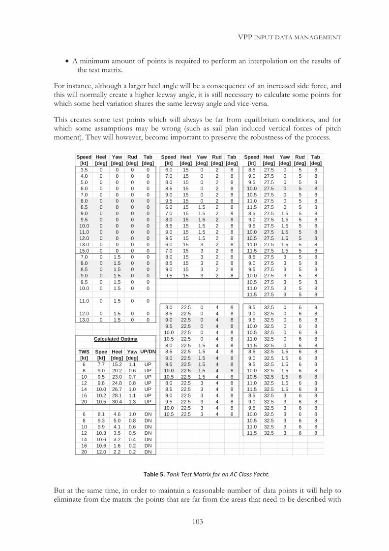
VPP INPUT DATA MANAGEMENT
103
A minimum amount of points is required to perform an interpolation on the results of the test matrix.
For instance, although a larger heel angle will be a consequence of an increased side force, and this will normally create a higher leeway angle, it is still necessary to calculate some points for which some heel variation shares the same leeway angle and vice-versa.
This creates some test points which will always be far from equilibrium conditions, and for which some assumptions may be wrong (such as sail plan induced vertical forces of pitch moment). They will however, become important to preserve the robustness of the process.
But at the same time, in order to maintain a reasonable number of data points it will help to eliminate from the matrix the points that are far from the areas that need to be described with
Table 5. Tank Test Matrix for an AC Class Yacht.
Speed Heel Yaw Rud Tab Speed Heel Yaw Rud Tab Speed Heel Yaw Rud Tab[kt] [deg] [deg] [deg] [deg] [kt] [deg] [deg] [deg] [deg] [kt] [deg] [deg] [deg] [deg]3.5 0 0 0 0 6.0 15 0 2 8 8.5 27.5 0 5 84.0 0 0 0 0 7.0 15 0 2 8 9.0 27.5 0 5 85.0 0 0 0 0 8.0 15 0 2 8 9.5 27.5 0 5 86.0 0 0 0 0 8.5 15 0 2 8 10.0 27.5 0 5 87.0 0 0 0 0 9.0 15 0 2 8 10.5 27.5 0 5 88.0 0 0 0 0 9.5 15 0 2 8 11.0 27.5 0 5 88.5 0 0 0 0 6.0 15 1.5 2 8 11.5 27.5 0 5 89.0 0 0 0 0 7.0 15 1.5 2 8 8.5 27.5 1.5 5 89.5 0 0 0 0 8.0 15 1.5 2 8 9.0 27.5 1.5 5 8
10.0 0 0 0 0 8.5 15 1.5 2 8 9.5 27.5 1.5 5 811.0 0 0 0 0 9.0 15 1.5 2 8 10.0 27.5 1.5 5 812.0 0 0 0 0 9.5 15 1.5 2 8 10.5 27.5 1.5 5 813.0 0 0 0 0 6.0 15 3 2 8 11.0 27.5 1.5 5 815.0 0 0 0 0 7.0 15 3 2 8 11.5 27.5 1.5 5 87.0 0 1.5 0 0 8.0 15 3 2 8 8.5 27.5 3 5 88.0 0 1.5 0 0 8.5 15 3 2 8 9.0 27.5 3 5 88.5 0 1.5 0 0 9.0 15 3 2 8 9.5 27.5 3 5 89.0 0 1.5 0 0 9.5 15 3 2 8 10.0 27.5 3 5 89.5 0 1.5 0 0 10.5 27.5 3 5 8
10.0 0 1.5 0 0 11.0 27.5 3 5 811.5 27.5 3 5 8
11.0 0 1.5 0 08.0 22.5 0 4 8 8.5 32.5 0 6 8
12.0 0 1.5 0 0 8.5 22.5 0 4 8 9.0 32.5 0 6 813.0 0 1.5 0 0 9.0 22.5 0 4 8 9.5 32.5 0 6 8
9.5 22.5 0 4 8 10.0 32.5 0 6 810.0 22.5 0 4 8 10.5 32.5 0 6 810.5 22.5 0 4 8 11.0 32.5 0 6 88.0 22.5 1.5 4 8 11.5 32.5 0 6 8
TWS Spee Heel Yaw UP/DN 8.5 22.5 1.5 4 8 8.5 32.5 1.5 6 8[kt] [kt] [deg] [deg] 9.0 22.5 1.5 4 8 9.0 32.5 1.5 6 86 7.7 15.2 1.1 UP 9.5 22.5 1.5 4 8 9.5 32.5 1.5 6 88 9.0 20.2 0.6 UP 10.0 22.5 1.5 4 8 10.0 32.5 1.5 6 8
10 9.5 23.0 0.7 UP 10.5 22.5 1.5 4 8 10.5 32.5 1.5 6 812 9.8 24.8 0.8 UP 8.0 22.5 3 4 8 11.0 32.5 1.5 6 814 10.0 26.7 1.0 UP 8.5 22.5 3 4 8 11.5 32.5 1.5 6 816 10.2 28.1 1.1 UP 9.0 22.5 3 4 8 8.5 32.5 3 6 820 10.5 30.4 1.3 UP 9.5 22.5 3 4 8 9.0 32.5 3 6 8
10.0 22.5 3 4 8 9.5 32.5 3 6 86 8.1 4.6 1.0 DN 10.5 22.5 3 4 8 10.0 32.5 3 6 88 9.3 5.0 0.8 DN 10.5 32.5 3 6 8
10 9.9 4.1 0.6 DN 11.0 32.5 3 6 812 10.3 3.5 0.5 DN 11.5 32.5 3 6 814 10.6 3.2 0.4 DN16 10.6 1.6 0.2 DN20 12.0 2.2 0.2 DN
Calculated Optima
VPP INPUT DATA MANAGEMENT
104
accuracy. Table 5 shows a standard tank test matrix in which speed, heel and leeway are varied. The highlighted points are the closest ones to calculated optima for different wind speeds, also shown in the table.
For the specific matrix shown in Table 5, which corresponds to an ACC yacht tank test, the effect of heel angle is important to evaluate, especially between 20 and 30 degrees, showing a change in its trend around 22.5 degrees. Behavior with leeway is very linear but it is not so much the case with heel, and certainly not with speed. A number of extra points are included to provide a double check of the trends in the lift curve slope and effective span. Clearly, many of them are points far from the equilibrium, but they help to identify those trends and confirm the slopes of the linear effects.
In addition to that matrix, which has fixed tab values and rudder angles linked to heel, a number of tab and rudder angle variations were included for the relevant speeds in different heel angles.
In some other cases, the test matrix is designed with the intention of generating a large amount of multi-parametric bulk data to build specific analytical models (such as the Delft series or a general-purpose sail model). This is more related to force modelling itself than to direct performance prediction, so it will not be discussed here in more detail. However, most of the discussed topics above would also apply to this situation.
Scaling up/down Matrix density
Whichever tools are used to evaluate forces, eventually it will be necessary to provide the VPP either with an analytical model based on the results or with an adequate data matrix along with an interpolation scheme capable of evaluating forces for each step of the calculation process.
Sometimes, forces may have clear dependencies on a small number of parameters, and a simple regression of the data can provide the coefficients necessary for the analytical formulae describing those forces.
In other cases, dependencies are far from evident and the cross effects between parameters make it difficult to establish an analytical model, and an interpolation scheme must be used. In these situations, the data matrix must be dense and extensive enough for the scheme to work. In most cases, a number of points in this matrix will need to be filled in, for which forces have not been evaluated. The matrices generated with the most “expensive” methods will be smaller, requiring that more voids be filled.
In these cases, the best process will depend on the available tools. But in general, the “expensive” and more accurate methods will help to correct results from the faster and less accurate methods, and the latter methods will help to expand results from the first ones into larger matrices.
Table 6 shows the matrix used for the study of the hull shape of an AC72 class yacht, in which the forces were evaluated using both a potential panel code with a non-linear free surface run with fixed sink and trim, and a RANSE code run in similar conditions. The first code would calculate a matrix of 142 points in six hours, and the second a matrix of 31 points in four days (in a large cluster; with similar computational power, the calculations would have taken months).
The matrix for the RANSE code corresponds to a detailed evaluation reserved for a select number of design candidates (a more ordinary check with just five points of the matrix would
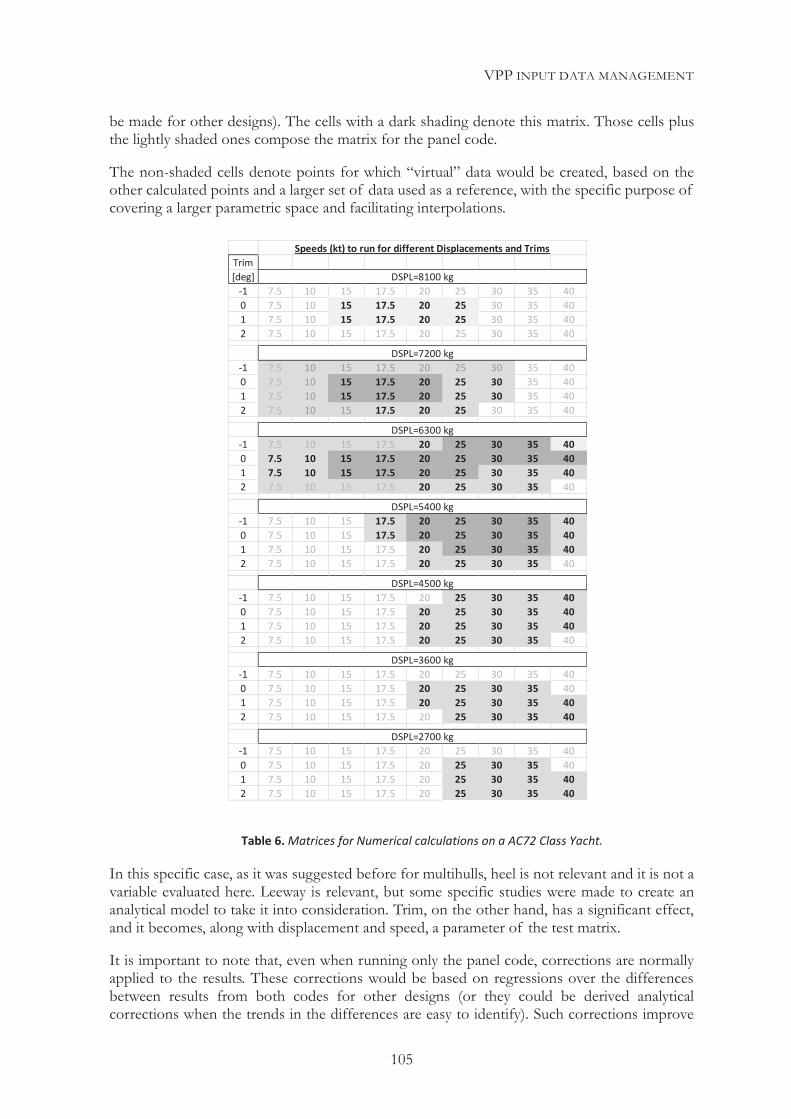
VPP INPUT DATA MANAGEMENT
105
be made for other designs). The cells with a dark shading denote this matrix. Those cells plus the lightly shaded ones compose the matrix for the panel code.
The non-shaded cells denote points for which “virtual” data would be created, based on the other calculated points and a larger set of data used as a reference, with the specific purpose of covering a larger parametric space and facilitating interpolations.
In this specific case, as it was suggested before for multihulls, heel is not relevant and it is not a variable evaluated here. Leeway is relevant, but some specific studies were made to create an analytical model to take it into consideration. Trim, on the other hand, has a significant effect, and it becomes, along with displacement and speed, a parameter of the test matrix.
It is important to note that, even when running only the panel code, corrections are normally applied to the results. These corrections would be based on regressions over the differences between results from both codes for other designs (or they could be derived analytical corrections when the trends in the differences are easy to identify). Such corrections improve
Table 6. Matrices for Numerical calculations on a AC72 Class Yacht.
Trim[deg]
-1 7.5 10 15 17.5 20 25 30 35 400 7.5 10 15 17.5 20 25 30 35 401 7.5 10 15 17.5 20 25 30 35 402 7.5 10 15 17.5 20 25 30 35 40
-1 7.5 10 15 17.5 20 25 30 35 400 7.5 10 15 17.5 20 25 30 35 401 7.5 10 15 17.5 20 25 30 35 402 7.5 10 15 17.5 20 25 30 35 40
-1 7.5 10 15 17.5 20 25 30 35 400 7.5 10 15 17.5 20 25 30 35 401 7.5 10 15 17.5 20 25 30 35 402 7.5 10 15 17.5 20 25 30 35 40
-1 7.5 10 15 17.5 20 25 30 35 400 7.5 10 15 17.5 20 25 30 35 401 7.5 10 15 17.5 20 25 30 35 402 7.5 10 15 17.5 20 25 30 35 40
-1 7.5 10 15 17.5 20 25 30 35 400 7.5 10 15 17.5 20 25 30 35 401 7.5 10 15 17.5 20 25 30 35 402 7.5 10 15 17.5 20 25 30 35 40
-1 7.5 10 15 17.5 20 25 30 35 400 7.5 10 15 17.5 20 25 30 35 401 7.5 10 15 17.5 20 25 30 35 402 7.5 10 15 17.5 20 25 30 35 40
-1 7.5 10 15 17.5 20 25 30 35 400 7.5 10 15 17.5 20 25 30 35 401 7.5 10 15 17.5 20 25 30 35 402 7.5 10 15 17.5 20 25 30 35 40
Speeds (kt) to run for different Displacements and Trims
DSPL=8100 kg
DSPL=7200 kg
DSPL=6300 kg
DSPL=5400 kg
DSPL=4500 kg
DSPL=3600 kg
DSPL=2700 kg
VPP INPUT DATA MANAGEMENT
106
the comparison of designs that have been evaluated with the two different methods (although not an ideal comparison, and rarely done).
The calculation of these corrections should be as automated as possible, but they require some verification with tools providing a proper graphic representation to detect unexpected trends.
In general, the corrections between methods should remain reasonably constant for different design alternatives, and they would normally be applied to the “faster” calculations for which no detailed alternative is available. However, they may change, and when these variations are significant, the tools used to evaluate the forces should be questioned and reviewed.
Matrix preparation for interpolation
The interpolation and extrapolation methods will also have an influence on the topology of the matrices for a number of reasons. Amongst them, the following ones should be taken into consideration:
Some methods may require rectangular matrices, and consequently a larger amount of data, although for a large part of this data, accuracy is not so much necessary as smoothness.
Extrapolation is always a potential problem, either because of the limitations of some methods to extend trends beyond the covered range of data, or because those trends do not respond to a moderate variation of the first or second derivatives. This may require the addition of data, beyond the original dataset, created with other methods that will be discussed later.
A minimum density/number of data points may be necessary for each dimension, along with requirements in terms of data spacing.
Methods which may be accurate and adequate for local interpolation may not be suitable as a global interpolation scheme.
All these reasons suggest that there should be specific methods in place to complete the data matrices with “virtual” data based on local trends. This is an efficient way to create sufficient coverage for the area of the parametric space in which the VPP will perform calculations, where interpolated or extrapolated values must be provided.
Matrices with a large number of dimensions
In those situations where a large number of parameters are involved (and consequently a large number of dimensions in the data matrices), it may be necessary to use different calculation strategies to define the desired data points for which the available tools will evaluate forces.
That would be the case when, in addition to the basic position and flow variables, a number of design parameters are evaluated across a range of design variations. This can happen, for instance, in parametric studies that use a specific set of data calculated for variations on a parent model, and which are used to perform optimization analyses.
In this situation, even if running a reasonably small matrix for each design, a large number of calculations is required, which may still only provide a limited assessment of the cross variations of the parameters of the study.
VPP INPUT DATA MANAGEMENT
107
The use of sparse matrices involving all the parameters may appear as a counter-intuitive solution, but it is an efficient way in this case to help limit the number of points to test or calculate, while still covering adequately a complex parametric space. However, this makes the interpolation more complicated, and the use of specific tools suitable to fit multidimensional sparse data (not organized as a regular grid), such as neural networks, may become necessary.
This also opens the door to techniques to derive data from an existent dense dataset corresponding to a previous design, based on a small number of test points for a new design. These techniques will be discussed at the end of this Chapter.
MODELLING DATA With the exception of pre-existent analytical models, forces will be evaluated only for a discrete number of points defined by the matrix of calculations when using experimental or numerical tools.
However, final solutions, as well as any step towards those results during the solving process, will happen in points of the parametric space different from those for which those forces are known. This implies the need to establish interpolation schemes, in order to provide a mechanism to evaluate forces in a continuous way throughout the range of interest of the parametric space. When doing this, some precautions must be observed.
5.2.1 PRECAUTIONS WHEN INTERPOLATING DATA
There are a large number of interpolation techniques to choose from, depending on the source of data, its behavior relative to the independent variables, the computational limitations, required smoothness and a number of other factors.
Some of them may significantly influence the accuracy and efficiency of the VPP calculation, and this must be taken into consideration when deciding what interpolation techniques to use.
Computational efficiency
Modern computers have enough power to make calculation times irrelevant when performing an interpolation over a set of data like the ones we are considering here. The problem is that forces are evaluated a large number of times in the VPP while searching for a solution. That is actually the part of the code where the VPP expends most of the calculation time (given that in addition to the multiple steps needed to solve the equilibrium, partial derivatives are calculated for each step).
Additionally, in time-domain calculations, even if most interpolation schemes will be sufficiently fast to allow calculations in real time, there is an inherent benefit in increasing the sampling rate at which they can be solved, or even in accelerating the process as much as possible when making a large number of simulations.
This favours methods where a pre-process is executed once (such as the calculation of a set of spline coefficients) before calculating equilibrium points; this takes some of the calculations out of the iterations.
VPP INPUT DATA MANAGEMENT
108
It is also advisable to generate some analytical models to account for the effects of some of the parameters, when possible and when the trends can be modeled with sufficient accuracy. For instance, eight data points knowingly aligned (other than some existent noise) can be fitted with a polynomial of order seven, but far from better capturing the data variations in between the points, that can create significant oscillations, in addition to multiplying the required calculation time.
Derivatives
The key for solving numerically non-linear equations is the calculation of derivatives. One of the factors which have a significant impact on the solving efficiency is the quality (in terms of smoothness) of those derivatives.
The physical phenomena involved in a sailing yacht have a continuous and smooth nature, with some specific exceptions in which qualitative changes happen. Having this favorable situation, it is important to guarantee that whichever interpolation method is used, at least the first derivative is of high quality in terms of smoothness. Otherwise, the last part of the solution may be difficult or even impossible to achieve using small calculation steps.
For instance, the simplest interpolation method may be a lookup table (the test matrix) providing a linear interpolation for intermediate values. This may be very accurate if the density of the matrix is high enough. But unless the data has a perfectly linear behavior (and in that case a linear regression would provide a much simpler interpolation scheme), the derivative of the evaluated function will be discontinuous, and will possibly show a large change between two close values situated on either side of a point of the table.
But a non-continuous first derivative is not the only source of issues. Oscillating first derivatives may have equally damaging or worse effects, depending on the period of the oscillations relative to the calculation step used by the solvers. This strongly suggests that special attention must be paid to avoid artificial introduction of those numerical oscillations, when choosing and/or implementing the interpolation algorithms.
Data with noise
The decision whether to smooth data prior to interpolation or with the interpolation algorithm is a difficult one. Data of experimental origin has a higher inherent level of noise than its numerical counterpart, but noise may be present no matter how the forces are calculated. Fortunately, in most cases, the noise is small compared to how much the forces change between two adjacent matrix points , and if that is the case, no smoothing may need to be applied.
However, sometimes the data may need to be faired prior to a final interpolation. As little practical as it may sound, an interactive process with verification on the results is highly recommended. In case of an extended and homogeneous level of noise across the parametric space, some fairing algorithms may be used.
The most significant risk is to over-smooth some “bumps” which may correspond to physical phenomena. This is the case sometimes with residuary drag, or keel/rudder interference with the free surface. In these situations, for some specific Froude numbers, characteristic wave interaction patterns may occur that change the forces locally. Some of this may be anticipated for some ranges of speeds, and special attention can and must be paid when these happen.
VPP INPUT DATA MANAGEMENT
109
With experimental results, if repeated points (or similar speed points with other parametric values) show the same result, the answer is very clear since the forces present are directly measured. With numerical tools, the answer may be more difficult to find, and it is necessary to rely on the expertise of the analyst to exclude numerical sources of noise, sometimes due to changes in the mesh topology or density.
No clear rules can be established to face this problem, but at least it is important to raise awareness about its existence, to give it a proper consideration.
Noise from computations
Although the available maximum precision for variables in most programming languages has increased over the years, numerical noise can still be a problem with interpolation and numerical calculations.
This can translate into increased errors in the interpolated values, but it has a much more damaging effect on their derivatives, to the point that it may even compromise the convergence of the solving process in the VPP.
This noise can be controlled albeit not eliminated, by taking some cautions when performing interpolations:
Always use in the calculation of interpolation coefficients the highest precision variables available for floating point calculations.
Pay special attention to data type or precision conversions, avoiding implicit conversions.
Avoid matrix inversions if possible or at least pay special attention to the methods used and their effects on data. Never assume that an available numerical method which provides a solution is free from computational noise. Depending on the elements of the matrix (placement or homogeneity of the values), the noise may be present or not.
Avoid combining very large numbers with very small ones. When there are differences between the orders of magnitude of different variables, use normalizing factors prior to interpolation (and after, to restore the actual values). Homogeneous numbers help significantly to preserve the maximum possible number of significant digits through the calculations.
The above cautions should help to prevent problems associated with computational noise, but, especially when new methods or different type of data is used, the results must be checked with special attention to the derivatives, visualizing bi-dimensional cuts in different dimensions, and if possible with an amplification of the noise in its graphical representation.
Extrapolation
Most interpolation algorithms either will not be able to extrapolate points outside the range of the input data or will lack control on the extrapolated data. This needs to be taken into consideration.
These are two simple methods to manage this problem:
VPP INPUT DATA MANAGEMENT
110
The first one, for those algorithms which permit extrapolation, consists in evaluating the behavior beyond the last input point of the range or artificially adding a continuity algorithm. Some control can be added by keeping constant the value of the function at that last point, or its first or second derivative. This may sometimes be an acceptable solution, when for instance keeping a constant first derivative will maintain the trend of the data, providing valid values for the solvers to work properly.
The second method consists in adding “virtual” data points to extend the range of the parameters, based on the local trends at the boundaries of the original data set. To do this, simpler and more robust ad-hoc algorithms can be used to create this “virtual” data, sometimes even manually tweaking them to comply with the basic criteria of maintaining the continuity and trends. When doing this outside of the VPP convergence area, The virtual data should be chosen so as to “push” the solvers back toward the range of data of interest. This is a reliable solution, and with some methods that are heavily affected by the boundaries of the data, like the neural networks, it is the only viable one.
Shape of the test matrices
An optimal test matrix will not be rectangular. Data points will be skewed in some variables and clustered around the areas where convergence is expected to happen or larger variations in the data trends take place. Even if ample margins are given around those points, the data rarely fills completely rectangular matrices (except in the cases where calculating that data is fast and reliable enough through the whole range of interest).
Some interpolation methods may be able to deal directly with these irregular sets of data, but in general, interpolating on regular rectangular matrices is preferable, even if it means adding points which are far from the areas of interest for the VPP.
The solution to this problem is similar to the second one given for the extrapolation problem. It consists in using “virtual” data, based on local trends in the existent data set.
Multidimensional interpolation, in which successive one-dimensional interpolations are used (the most common situation), is one of the reasons why regular rectangular matrices are usually desirable. However, some algorithms permit direct multidimensional interpolation over sparse data. If this is the case, it becomes a factor that can condition the actual test matrix and that may allow reducing its size.
Non-dimensionalization.
Although in most cases the use of non-dimensionalized forces is not a requirement, it is normally preferable to eliminate the speed factor by dividing forces by the dynamic pressure, which is calculated as:
where and V are respectively the density and speed of the fluid.
This has little impact in the interpolation, except in the range of speeds close to zero, where it makes it easier to observe the trends in the drag coefficients, by removing a certain “masking factor” from the speeds. This permits a better evaluation of the changes in the coefficients with
Equation 15. Calculation of the dynamic pressure.
VPP INPUT DATA MANAGEMENT
111
speed, and facilitates visual inspection of a graphic representation of the data by reducing its range of variation.
5.2.2 SUITABLE INTERPOLATION TECHNIQUES
In order to provide algorithms that permit the calculation of forces anywhere in the range of interest of the parametric space, different interpolation techniques can be used based on the available data points.
Regression to parametric models. Functional fitting
In some cases, the reduced amount of data available, or the fact that some dependencies on the test variables may be well known, suggest a clear path for estimating the effect of those variables on the forces. This may require only the calculation of the coefficients for some regressions, which may correspond to some of the algorithms described below (mostly polynomial ones).
For instance, with some degree of simplification, it can be assumed that the effective span of the appendages does not change with speed and has a value that is only a function of heel (certainly an over-simplification when the appendages are close to the free surface with heel).
Another example of this would be the following functional fit proposed by A. Claughton (7) for the calculation of drag, which includes the heeled drag, as a function of the upright drag (RU), speed and heel angle, and the induced drag as a function of the side force (FH), speed and heel angle, along with a full upright drag curve:
The coefficients C1 to C8 need to be calculated by a regression analysis on the available data, which could also be a weighted fit favoring the points close to where convergence is expected.
However, whichever data fit strategy is chosen, the forces calculated with the resultant model should be compared to the original data points to assess whether the error is acceptable, no undesirable smoothing takes place, and the trends are preserved in the whole area of the parametric space where the VPP is expected to perform evaluations.
The drawback of these methods is that they artificially smooth the data, removing those effects not strictly following the implicit dependencies embedded in the proposed model. One case where the previous example may over-simplify data is when the yacht sails at high heel angles and the interference of the lifting keel with the free surface is significant and variable with the Froude number (with wave interaction effects beyond linear or quadratic dependencies).
Still, this is a valid solution for interpolating small sets of data. It is also effective for force modifiers, like for instance those capturing the effect of variation from default values in the linked parameters. Those force modifiers are normally built using data close to the points of interest where the VPP is expected to find solutions; therefore, their accuracy tends be good in that region of the parametric space. Further away from the VPP convergence region where the
Equation 16. Functional fit for Total Drag with Upright, Heeled and Induced Drag components.
VPP INPUT DATA MANAGEMENT
112
variations were tested, errors in the force modifier models may be larger, but since the errors are relative to the magnitude of the force modifier, which is a small portion of the total force, the impact of such errors on the global forces will normally remain small and consistent.
Also in those situations, the correlation of forces may be strongest with one specific parameter, as would be the case for the relation of lift to leeway angle for a given speed and heel angle. In this specific example a linear relationship with leeway may be assumed, only requiring to additionally model the variations of the slope and the zero lift point with heel (which affects mostly the zero lift point) and speed (which affects mostly the slope).
In general, functional fitting provides models with continuous and fair data and first derivatives.
Polynomial interpolation
When the amount of data is larger in one dimension than in others and/or the trends are not linear, the next step is to consider polynomial interpolation of various degrees. However, with orders beyond cubic, there is a high risk of oscillations, especially at the edges of the interpolation domain if using equidistant interpolation points (Runge’s phenomenon (44)).
These oscillations can affect the data accuracy, but even more significantly, they get amplified in the derivatives, compromising the solving process in the VPP.
This tends to limit the use of polynomial interpolation to quadratic or cubic orders. It is used mostly with clean data in which the second derivative has low values at the edges of the interpolation domain; otherwise, data extrapolation may lead to unrealistic values. It is highly recommended to avoid the use of polynomials of higher order than cubic.
Spline interpolation
This is a form of interpolation based on the use of a type of piecewise polynomials called splines, which has the advantage of small interpolation errors while using well-behaved low degree polynomials.
The name is derived from the flexible rulers, used to draft line plans, as the original concept was developed to reproduce the bending characteristics of these rulers. A spline passes through the interpolating points, and between these points in between assume a shape of least deformation energy. In order to achieve this, polynomials of degree three or higher are used. While different degrees of polynomials can be used, cubic splines are most commonly used.
A cubic spline is a function constructed of piecewise third-order polynomials, which passes through a set of n control points, and which is continuous and has continuous derivatives up to the second derivative. In addition, the second derivative of the function at the endpoints of the interpolation domain is set to a given value, providing a boundary condition that completes the system of n-2 equations.
This value is commonly chosen as zero, producing a so-called "natural" cubic spline and leading to a simple tri-diagonal system, which can be solved easily to obtain the coefficients of the polynomials. However, other choices of boundary condition at the endpoints can be made.
These splines are twice differentiable, guarantee a smooth connection between the pieces at the interpolating points, and present the stability associated to the low order polynomials used.
VPP INPUT DATA MANAGEMENT
113
This flexibility, a certain degree of control at the ends, the smoothness associated to the low order polynomials used, and the continuity conditions at the data points, make them an excellent choice for interpolating variables over a high number of samples, especially in those cases where no clear trends are expected and the level of noise is low..
There is no need for the data to be equally spaced, but the values of the independent variable need to be monotone increasing. Also, it is advisable to verify the fit in areas where the data changes significantly for close points, as it may induce oscillations. The influence of data on local oscillations can be expected to be similar to that of cubic polynomials, given that such polynomials constitute the different “pieces” of the spline.
Multi-variable interpolation
When dealing with multiple parameters, it is usual to model the effect of some of them via force modifiers. However, the normal situation is that interpolations need to be made in different dimensions, such as speed, heel and yaw. In this case, it is necessary to interpolate in several independent variables.
There are different techniques to do this, but in general, the cubic splines are still a good solution. Bi-cubic or tricubic interpolation can be used.
When the data is structured in a regular rectangular grid, there is no difference between performing a global bicubic interpolation or making successive one-dimensional interpolations in each variable. This tends to be the normal choice given that computing times are similar.
However, there are situations where the data distribution is sparse with a good presence over the whole parametric space. In this case, using a method that permits simultaneous interpolation in two or three dimensions may allow for a more robust scheme. If this is possible, it allows using a smaller number of data points instead of requiring full matrices with a regular grid.
Fairing Splines
There are cases in which some level of noise is expected, while the physical phenomenon is known to behave in a fair manner. Then it may be tempting to use fairing techniques, but as stated before, special care must be taken not to over-smooth the data.
When the number of data points is small, it is possible to fit using least-squares regression a low order polynomial, which may provide the required amount of fairing, especially when the data is expected to have a linear, quadratic or even cubic behavior. However, if the number of data points is higher, splines are a useful fairing tool.
Different algorithms are available for this task, which offer different degrees of control and sometimes permit to limit the deviation from each one of the actual data points. This allows different levels of confidence to be set for each point to prevent specific data features from being smoothed. This is the most robust and recommended choice.
B-splines (Basis-Splines) or in general NURBS (Non-Uniform Rational B-Splines) curves or surfaces are in general a good method for fairing data. They provide an easily controllable network of control points for which the degree of control of each individual control point can be adjusted.
But whichever method is used, rather than leaving this final fairing interpolation to the VPP, the clear recommendation is to perform the data fairing in advance, when its effects can be verified,
VPP INPUT DATA MANAGEMENT
114
and then derive from this process a modified matrix of faired data to perform a simple interpolation over it. This reduces the ambiguity on the final interpolated data and allows a more generalized treatment of the data inside the VPP.
Neural networks
Neural networks (NN) can be used to interpolate data where the number of variables is large, and especially when that data is not organized as a regular grid.
With a very different approach from other data fitting methods, neural networks are non-parametric models, so there is no need to choose the functional form for each dimension. On the other side, as a non-parametric approach, they present a risk of over-fitting to noise or errors in the data. However, they are adequate to model the complete range of interest of the parametric space, and that is one of their main strengths.
As A. Mason describes in his thesis (45), since neural networks learn by example, they do not require the traditional statistical assumptions such as constant error variance and Gaussian distribution of errors. Instead, the neural network user gathers representative data and invokes training algorithms to learn the structure of the data. A number of tools to automate this process, as well as to evaluate the quality of the results, are commercially available.
If it is planned to use neural networks, it should be taken into consideration when designing the experiment, in order to define the data points both for the training process and for the evaluation of the results. Ideally, the data points should have a quasi-random distribution throughout the parametric space. The Uniform Design method, proposed by Fang (46), is a robust solution for this task, when neural networks will be the chosen method for fitting and interpolating data.
Special attention must be given to the fact that neural networks have an unpredictable behavior for extrapolation beyond the boundaries of the data used for training. Beyond those points, hypersurfaces can deform in ways that can render any extrapolated values useless, and that can even affect data and trends close to the boundaries but still inside them. For this reason, it is a common precaution to expand the base data beyond the boundaries of interest or create “virtual” data using other methods, in order to extend the area in which the results are adequate.
Given the complexity associated to them and the fact that the training process can be time consuming, neural networks are not a usual choice. One notable exception happens in cases in which a multi-parametric analysis of design candidates, involving geometric parameters, is performed over a set of variations from a parent boat. Then, this original “fleet” is used to feed an optimization analysis intended to explore a larger range of parameters combinations.
In this case, the most efficient procedure consists in not discriminating between the position and flow parameters (basically the choice of speed, heel, yaw, trim, displacement, etc. adequate for the type of yacht) and the geometrical parameters being altered (such as variations of beam, form coefficients, length, etc.).
Then, a limited number of design alternatives are created with different combinations of the geometric parameters, and are analyzed for a number of combinations of the position and flow parameters, so that the global distribution of the full set of combinations fills the design space in a quasi-random way. The total number of points will depend on the method used for their calculation (in this case the most reasonable option is a numerical tool), and the desired balance of time versus the degree of simplification.
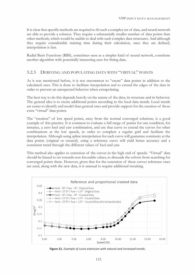
VPP INPUT DATA MANAGEMENT
115
It is clear that specific methods are required to fit such a complex set of data, and neural network are able to provide a solution. They require a substantially smaller number of data points than other methods, which would be unable to deal with such complex data structures. And although they require considerable training time during their calculation, once they are defined, interpolation is fast.
Radial Basis Functions (RBS), sometimes seen as a simpler kind of neural network, constitute another algorithm with potentially interesting uses for fitting data.
5.2.3 DERIVING AND POPULATING DATA WITH “VIRTUAL” POINTS
As it was mentioned before, it is not uncommon to “create” data points in addition to the calculated ones. This is done to facilitate interpolation and to extend the edges of the data in order to prevent an unexpected behavior when extrapolating.
The best way to do this depends heavily on the nature of the data, its structure and its behavior. The general idea is to create additional points according to the local data trends. Local trends are easier to identify and model than general ones and provide support for the creation of those extra “virtual” data points.
The “creation” of low speed points, away from the normal converged solutions, is a good example of this practice. It is common to evaluate a full range of points for one condition, for instance, a zero heel and yaw combination, and use that curve to extend the curves for other combinations at the low speeds, in order to complete a regular grid and facilitate the interpolation. Although using spline interpolation for each curve will guarantee continuity at the data points (original or created), using a reference curve will yield better accuracy and a consistent trend through the different values of heel and yaw.
This method also applies to extension of the curves in the high end of speeds. “Virtual” data should be biased to err towards non-favorable values, to dissuade the solvers from searching for converged points there. However, given that for the extension of these curves reference ones are used, along with the new data, it is unusual to require additional tweaking.
Figure 21. Example of curve extension with natural and increased trends.
VPP INPUT DATA MANAGEMENT
116
Figure 21 shows an example where a reference curve at zero heel and yaw is used to extend a tank test shorter curve, for 27.5 degrees of heel and 1.5 degrees of yaw, with a natural extension or with a forced pessimistic factor in the high speeds end. Trends and smoothness are preserved, which is the main requirement not to affect the efficiency of the solvers.
Given the skewed nature of the matrices on some parameters, “virtual” data may need to be created in a similar manner to complete a full rectangular grid.
In most cases, the trends in variables such as yaw and heel are simpler (hence the smaller number of points), from a linear trend of lift with yaw, to something close to a quadratic dependence on heel.
It is important to take advantage of any known relationships that may simplify the “guesses” for the trends. For instance, the induced drag will not change linearly with yaw but it will remain approximately constant in relation to the squared generated lift when yaw changes, via the calculated effective span. In this case, the reasonable option is to extend the data by maintaining the trend in the effective span, i.e. no dependency on leeway and a simple correlation with heel
Known relationships should be used to look for the simplest possible trends (which will also help to assess the rate of change of some relevant relationships), because the “virtual” data must be fair relative to all variables.
The example shown in Figure 21 is taking into consideration only the speed, but those “virtual” points must also maintain the trends across the other test variables. Ideally, all trends would converge to the same values, but this will never happen, as there will be implicit noise in the data. The simplest solution is to take an average (or weighted average if needed) of the projected values for the “virtual” points for each variable.
This is one of the situations where data visualization allows making use of the human ability for pattern recognition. Having either a dedicated tool or just a simple spreadsheet for the “creation” of data, with automated formulas that can be tweaked and with some significant plots showing the trends, allows to make this process easier, safer and more systematic.
It is important to remember that it is preferable to maintain the trends and smoothness to facilitate interpolation than to try to have very accurate values for the “virtual” data (certainly desirable but not at all costs) away from the range of solutions.
A. Claughton refers to “judicious human touch” (7) as a requirement for extracting a rationale functional fit from a set of sparse data. This criterion also applies when creating “virtual” data.
5.2.4 A PROPOSED INTERPOLATION STRATEGY
The best interpolation scheme depends on the shape of the data. Its topology, number of dimensions, distribution over the parametric space, clustering, etc., will determine the best methods, but the following points can help to establish a solid base for the calculation of forces for the VPP:
Whenever simple correlations are expected, they should be used regardless of the amount of data. Five points in line with a good correlation do not require a high degree polynomial or spline but a least-squares fitted line, which will most likely have its slope defined by a physical parameter (such as an effective span).
VPP INPUT DATA MANAGEMENT
117
Whenever the effect of some parameters is well known (mainly, but not limited to, the previously called “linked parameters”) and can be accurately described by a functional fit, this option should be used, removing that variable from the general interpolation. This helps to preserve accuracy and speed up calculations.
When parameters can be combined into transformed variables that have a physical meaning, the transformed variables should be used rather than the original ones. For instance, lift slope or effective span, besides having a physical meaning, have a more predictable trend than lift or drag.
Cubic splines are a good base for variables with a number of points higher than four or five; the speed of the yacht is a good example of an adequate candidate variable. Whenever cubic splines are used in different dimensions, it is important for computational efficiency to start with the dimension that has the largest number of data points (usually speed) and calculate the spline coefficients in that variable for each combination of the other variables, as part of the pre-processing in the VPP. This way, the spline interpolation in that variable can be used every time forces are evaluated without requiring a recalculation of the corresponding spline coefficients.
Even in cases when the number of points permits to fit a low degree polynomial, it should be considered whether it is preferable to use a spline with imposed conditions on the derivatives at the ends, providing a more robust and predictable extrapolation scheme. The decision of whether it is justified to use extra computational effort depends strongly on the implicit smoothness of the data.
For subsequent interpolations, for which the coefficients cannot be calculated in advance, one option is to prepare as part of the pre-processing a dense regular grid in the direction of every independent variable, for instance using splines. Then, for each point to interpolate, the closest point in the grid is selected and the adjacent points are used for a low degree polynomial interpolation (usually parabolic) that will provide low errors if the grid is dense enough; and as long as the step taken by the solver when calculating derivatives is of a lower order than the grid spacing and the data is smooth, the errors and noise in calculated derivatives will be negligible. In addition, the search for the next base point in the table will be very fast. This solution was originally used by J. Ozanne in the search for faster interpolation methods. It permits to speed up significantly the evaluation of forces.
Normalizing factors should be used on the final variables (original or derived) to be interpolated, in order to minimize computational noise coming from precision issues.
When data needs to be faired, it should be done as part of a preparation for a final set of data to be interpolated, in order to maintain control over the degree of fairing applied.
The results of the interpolations should be inspected, especially when changes are made on proven methods, data topologies or densities, paying special attention to the smoothness of the first derivatives.
The same interpolation procedures (and ideally, data structure) should be used when making comparative evaluations within a design decision process.
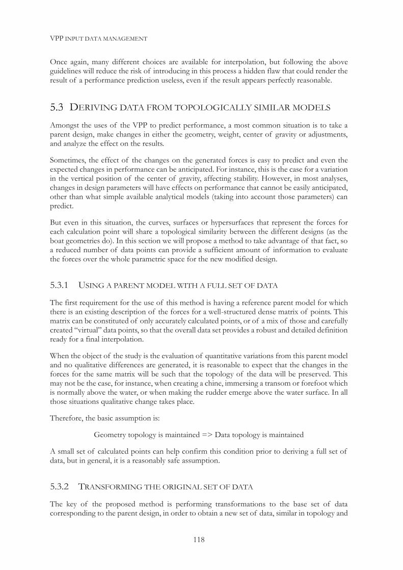
VPP INPUT DATA MANAGEMENT
118
Once again, many different choices are available for interpolation, but following the above guidelines will reduce the risk of introducing in this process a hidden flaw that could render the result of a performance prediction useless, even if the result appears perfectly reasonable.
DERIVING DATA FROM TOPOLOGICALLY SIMILAR MODELS Amongst the uses of the VPP to predict performance, a most common situation is to take a parent design, make changes in either the geometry, weight, center of gravity or adjustments, and analyze the effect on the results.
Sometimes, the effect of the changes on the generated forces is easy to predict and even the expected changes in performance can be anticipated. For instance, this is the case for a variation in the vertical position of the center of gravity, affecting stability. However, in most analyses, changes in design parameters will have effects on performance that cannot be easily anticipated, other than what simple available analytical models (taking into account those parameters) can predict.
But even in this situation, the curves, surfaces or hypersurfaces that represent the forces for each calculation point will share a topological similarity between the different designs (as the boat geometries do). In this section we will propose a method to take advantage of that fact, so a reduced number of data points can provide a sufficient amount of information to evaluate the forces over the whole parametric space for the new modified design.
5.3.1 USING A PARENT MODEL WITH A FULL SET OF DATA
The first requirement for the use of this method is having a reference parent model for which there is an existing description of the forces for a well-structured dense matrix of points. This matrix can be constituted of only accurately calculated points, or of a mix of those and carefully created “virtual” data points, so that the overall data set provides a robust and detailed definition ready for a final interpolation.
When the object of the study is the evaluation of quantitative variations from this parent model and no qualitative differences are generated, it is reasonable to expect that the changes in the forces for the same matrix will be such that the topology of the data will be preserved. This may not be the case, for instance, when creating a chine, immersing a transom or forefoot which is normally above the water, or when making the rudder emerge above the water surface. In all those situations qualitative change takes place.
Therefore, the basic assumption is:
Geometry topology is maintained => Data topology is maintained
A small set of calculated points can help confirm this condition prior to deriving a full set of data, but in general, it is a reasonably safe assumption.
5.3.2 TRANSFORMING THE ORIGINAL SET OF DATA
The key of the proposed method is performing transformations to the base set of data corresponding to the parent design, in order to obtain a new set of data, similar in topology and
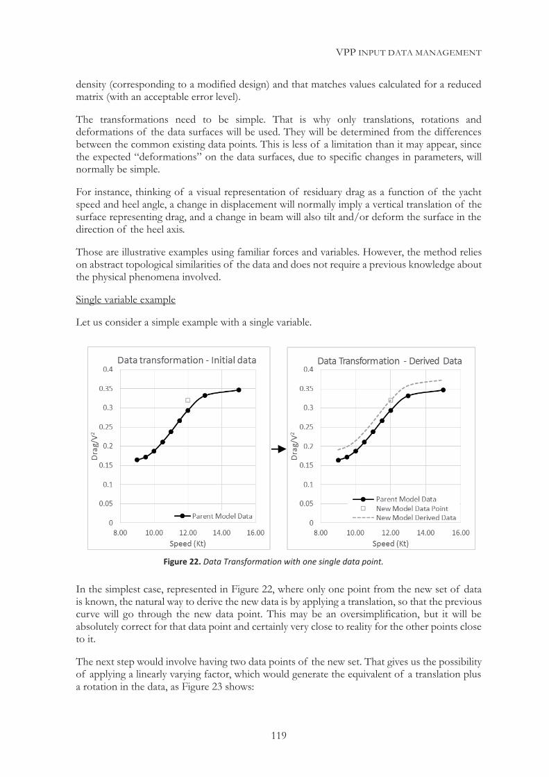
VPP INPUT DATA MANAGEMENT
119
density (corresponding to a modified design) and that matches values calculated for a reduced matrix (with an acceptable error level).
The transformations need to be simple. That is why only translations, rotations and deformations of the data surfaces will be used. They will be determined from the differences between the common existing data points. This is less of a limitation than it may appear, since the expected “deformations” on the data surfaces, due to specific changes in parameters, will normally be simple.
For instance, thinking of a visual representation of residuary drag as a function of the yacht speed and heel angle, a change in displacement will normally imply a vertical translation of the surface representing drag, and a change in beam will also tilt and/or deform the surface in the direction of the heel axis.
Those are illustrative examples using familiar forces and variables. However, the method relies on abstract topological similarities of the data and does not require a previous knowledge about the physical phenomena involved.
Single variable example
Let us consider a simple example with a single variable.
In the simplest case, represented in Figure 22, where only one point from the new set of data is known, the natural way to derive the new data is by applying a translation, so that the previous curve will go through the new data point. This may be an oversimplification, but it will be absolutely correct for that data point and certainly very close to reality for the other points close to it.
The next step would involve having two data points of the new set. That gives us the possibility of applying a linearly varying factor, which would generate the equivalent of a translation plus a rotation in the data, as Figure 23 shows:
Figure 22. Data Transformation with one single data point.
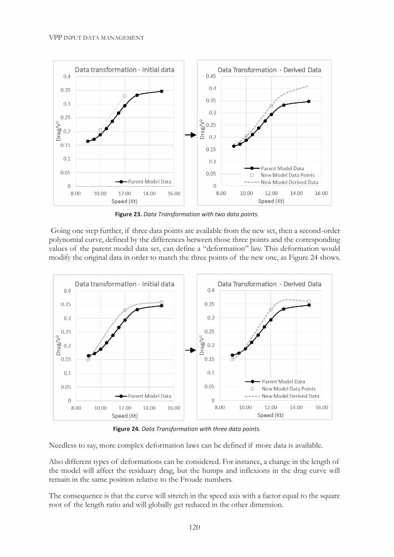
VPP INPUT DATA MANAGEMENT
120
Going one step further, if three data points are available from the new set, then a second-order polynomial curve, defined by the differences between those three points and the corresponding values of the parent model data set, can define a “deformation” law. This deformation would modify the original data in order to match the three points of the new one, as Figure 24 shows.
Needless to say, more complex deformation laws can be defined if more data is available.
Also different types of deformations can be considered. For instance, a change in the length of the model will affect the residuary drag, but the humps and inflexions in the drag curve will remain in the same position relative to the Froude numbers.
The consequence is that the curve will stretch in the speed axis with a factor equal to the square root of the length ratio and will globally get reduced in the other dimension.
Figure 23. Data Transformation with two data points.
Figure 24. Data Transformation with three data points.
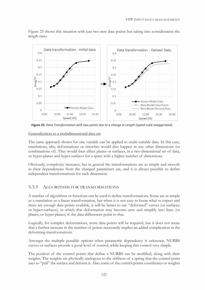
VPP INPUT DATA MANAGEMENT
121
Figure 25 shows this situation with just two new data points but taking into consideration the length ratio.
Generalization to a multidimensional data set
The same approach shown for one variable can be applied to multi-variable data. In this case, translations, tilts, deformations or stretches would also happen in any other dimensions (or combinations of). They would then affect planes or surfaces, in a two-dimensional set of data, or hyper-planes and hyper-surfaces for a space with a higher number of dimensions.
Obviously, complexity increases, but in general the transformations are as simple and smooth as their dependencies from the changed parameters are, and it is always possible to define independent transformations for each dimension.
5.3.3 ALGORITHMS FOR TRANSFORMATIONS
A number of algorithms or functions can be used to define transformations. Some are as simple as a translation or a linear transformation, but when it is not easy to know what to expect and there are enough data points available, it will be better to use “deformed” curves (or surfaces, or hyper-surfaces), in which that deformation may become zero and simplify into lines (or planes, or hyper-planes) if the data differences point to that.
Logically, for complex deformations, more data points will be required, but it does not mean that a further increase in the number of points necessarily implies an added complication in the deforming transformations.
Amongst the multiple possible options when parametric dependency is unknown, NURBS curves or surfaces provide a good level of control, while keeping this control very simple.
The position of the control points that define a NURBS can be modified, along with their weights. The weights are physically analogous to the stiffness of a spring that the control point uses to “pull” the surface and deform it. Also, some of the control points coordinates or weights
Figure 25. Data Transformation with two points due to a change in Length (speed scale exaggerated).
VPP INPUT DATA MANAGEMENT
122
can be constrained. For example, in the case of a NURBS surface built on a three-dimensional space, the coordinates of the control points in dimensions corresponding to the two independent variables can be fixed while the "vertical" position of the control point, affecting the data variable, is free. The value of the weight of the control point can also be constrained.
A least-squares regression can provide the best set of displacements for the control points, minimizing the errors between the deformed surface and the new data points.
Imposing limitations on the number of control points or the order in each dimension can guarantee that the deformation will be as simple and smooth as desired.
In addition, the control points can be positioned and/or clustered in zones where the original data must undergo larger deformation to fit the new data points, facilitating the control in those zones that require it. A look at the fit errors can also give an indication of where those control points should be re-placed to make a better fit of the transformation.
This combination of control and simplicity makes the NURBS a good choice for this task.
If the number of new data points is high and the number of variables is more than two or three, neural networks or radial basis functions are good candidates to fit the deformation function, especially if the data does not form a regular grid.
The possibilities for this method are very promising, but it requires further work to provide standardized procedures of general application.
As a starting point, it has proven to work extremely well in the experience of this author. In an optimization study, it permitted to replace repetitive test matrices of 65 points per design variation by an initial matrix for the parent model with 140 points (that were expanded to a regular grid of over 200 points) and 22 points for each successive variation. This allowed generating automatically dense matrices with good data quality for each one of them, by deforming the data corresponding to the parent design. Globally, this approach permitted to reduce by two thirds the time required to obtain results.
SOLVING FOR A SAILING CONDITION
123
6| SOLVING FOR A SAILING CONDITION After reviewing the nature of the equilibrium and motions for a sailing yacht, as well as the calculation of the forces involved, the next step is to analyze how those forces condition the kinetic and kinematic behavior of the yacht. Determining how those forces will be balanced will define the type of solution to be calculated and the circumstances and restrictions under which that calculation will be performed.
In the most conventional (and common) case, the type of solution will consist in an optimum stationary-state sailing point for some given environmental conditions. It will include a definition of the position and velocity of the yacht, along with final values for any adjustable parameters that were optimized in the process.
However, it is also possible to calculate the motion of the yacht under unstable or varying environmental conditions or adjustments. In this case, instead of having a zero-sum balance of forces, there will be an imbalance of forces and/or moments that will induce motions. In reaction to those motions, some sailing parameters may be adjusted through time, reproducing how the yacht is normally sailed, with human intervention or by means of autopilots.
All these possibilities require different solving strategies, as well as different actions associated to the solving process. These will be the core of this Chapter.
VARIABLES AND CONSTRAINTS Several variables will be involved in the normal solving process, and even in the simplest case, some of them can be adjusted independently, whether they are managed by the VPP in the search for the optimum or not. Other variables will be a function of others and their values will change through the different steps taken towards the solution. Most of them will have their values either bounded or constrained by conditions that will limit how and when they can change.
Sometimes, the same variables will play different roles depending on the type of analysis performed. For that reason, their nature and their potential interactions are discussed here in more detail.
6.1.1 VARIABLES
We will start by identifying the relevant variables involved in the solving process and discussing their expected behavior.
In the traditional approach to VPP solving, the variables in play can be divided in two types: state and decision variables. The state variables define the yacht position and speeds at which equilibrium takes place. The decision variables are parameters subject to optimization (usually depowering adjustments).
While this is a common approach, it has the disadvantage that it establishes a-priori the nature of the variables, making it difficult to define a generalized solution process.
SOLVING FOR A SAILING CONDITION
124
For this reason, this strict distinction between variables will be intentionally avoided, and the different roles of the variables will only be assigned when defining a specific problem to be solved.
The relevant variables can be classified in a number of different ways, but at this point we will start by referring to what their values describe. Based on that, some specific types can be established:
Variables that define the yacht along with its position and motions.
Variables that define adjustments made to the yacht.
Variables that define the environmental conditions.
Calculated variables function of others from the previous groups.
Let us discuss the different variables in some more detail, although some distinctions are often vague.
Variables that define the yacht along with its position and movements.
These are the minimum set of linearly independent state variables that characterize the state of a system (in this case the yacht) at a given time.
The basic set of state variables will define the yacht fitted for a default basic sailing condition, along with its attitude and kinematic condition for the situation being described.
This will include its geometric description along with how any on-board systems involving movement can be adjusted by the sailors. It must also comprises the mass properties, including center of gravity and inertias, as the mass state variables required to characterize the dynamic behavior of the yacht when subject to accelerations, or even just under the influence of hydrostatic forces.
Regarding the yacht’s position and motions, the space state variables will describe the position of the yacht in the six degrees of freedom, and the speeds and accelerations.
All the space variables will always be referred to a known convenient set of axes, in general the track or the design boat axes.
The relevance of each of the 18 values that will constitute the group of the space state variables will depend on the problem to be solved. However, the number of values of interest will be reduced to a much smaller number in many cases, such as when solving for a stationary state or in general for problems where the motions are constrained in some way.
Sometimes, the deformation of the yacht (departing from an initial solid-rigid condition) will need to be characterized as well, using deformation state variables. These deformations, produced as a consequence of the stresses, can be ignored in most cases, but there are some situations when they should be taken into consideration.
A clear example of this happens in multihulls, where torsion deformation in the Y-axis can be such that the trim angle of the windward hull can differ from that of the leeward hull by several degrees.
SOLVING FOR A SAILING CONDITION
125
The degree of torsion is strongly linked to the proportion of total displacement carried by the windward hull (from 50% to 0%) and it has some small aerodynamic implications. However, if the windward hull has any immersed foils close to horizontal, the change in their angle of attack relative to the corresponding appendage in the leeward hull cannot be ignored. In this situation, the torsional deformation may have significant implications on the calculation of vertical forces and associated pitch moments.
A subjective choice is made to consider as a different group the variables that change the positions of parts of the yacht, affecting its state. These are described below.
Variables that define adjustments
This group includes a specific set of state variables defining adjustments made to parts of the yacht, having an influence on the generated forces, equilibrium, and ultimately performance. We will denote them as adjustment state variables. The changes in their values may have effects on:
Weight or center of gravity (by moving weights or changing ballast).
Aerodynamic characteristics (by adjusting and/or depowering sails).
Hydrodynamic characteristics (by adjusting the position of appendages or parts of them).
Hydrostatic characteristics (by adjusting the position of appendages or parts of them).
Changing an adjustment variable may have some or all of these effects. Those variables can be considered as modifiers to the yacht state, and that is the reason for separating them from the main state variables.
This group will be constituted by the minimum set of linearly independent adjustment variables required to define those changes (they must also be linearly independent from other state variables). For instance, the degree of immersion of a lifting board changes a number of variables, but having the knowledge of the geometry and mechanism, a simple value as immersed length will be enough to define its state.
These variables are the clearest example of decision variables. In the process of performing a calculation, the VPP will search for the optimal combination of them that provide a valid solution.
Variables that define the environmental conditions
This group of variables will describe as a minimum the wind. When added resistance in waves or the influence of waves on the boat motions needs to be considered, the sea state will need to be characterized as well. Finally, when there is a current which needs to be taken into consideration, additional variables will be introduced to define it.
The wind will be defined by its vector, composed of the true wind speed (module) and angle (direction), along with a definition of the wind gradient. The wind will be assumed parallel to the surface of the water.
The system of reference normally used to define these variables will be the one defined by the track axes, with the true wind angle being also used to define the wind axes for the calculation of aerodynamic forces.
SOLVING FOR A SAILING CONDITION
126
An additional group of variables and constants will define physical properties of the fluids involved, such as temperatures, salinity, densities and viscosities. These last two values may be taken to the group of calculated variables as they can be estimated as a function of temperature and salinity.
The derived apparent wind variables will also be part of the calculated variables. In this case, the apparent wind will be calculated from the true wind and the relevant yacht space state variables (yacht speed and leeway), by solving the wind triangle.
Calculated Variables
This group includes all remaining variables which are adjusted during the solving process, not directly but as a consequence of changes in other variables of which they are a function. It comprises a wide range of variables, which can be grouped as follows:
Variables defining aero and hydrodynamic measurements and coefficients that depend on the yacht state and adjustments, that are directly used in the calculation of forces. Examples of such variables are the dynamic length and wetted surface.
Variables calculated as function of the state/decision variables, used or not in other intermediate calculations, as for instance a measurement of freeboard or transom immersion.
Variables defining the (apparent) incoming aero and hydrodynamic flows, depending on the yacht state and adjustments.
Any of these variables can become relevant for some specific analysis.
An example of analysis would be searching for the optimal sail settings that maximize the driving force for a fixed heel moment, relevant when the driving force is the objective function of the optimization but stability restrictions are in place. A similar case is the calculation of the flying condition in a multihull when the righting moment remains almost constant.
Another situation where these variables can condition the search of a solution is when the variable representing the freeboard in a specific location has bounds that represent limit conditions for capsizing, even if the performance is optimum in the frontier of the optimization (defined by variable bounds and constraints that will be discussed in the following section). The calculated values would help to define specific safety boundaries for the operational range of values of the yacht. Solutions outside those ranges can be permitted but would include specific warnings.
Although “hidden” among other calculated variables, forces and moments are the basis for the calculations of the equilibrium or motions of the yacht, but rather than being independent, they have a direct dependency on other independent variables, and that is the reason why they are included in this group.
Along with the apparent wind, forces and moments are probably the best example of how this specific classification of variables has no relationship with their actual relevance but rather with the role they play within the calculation process.
Table 7 provides a general summary of the variables involved in the solving process along with factors describing their nature and possible behavior based on the previous descriptions.
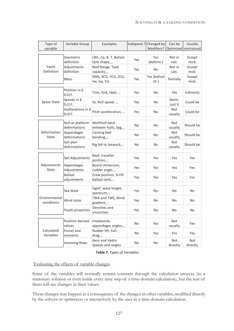
SOLVING FOR A SAILING CONDITION
127
Evaluating the effects of variable changes
Some of the variables will normally remain constant through the calculation process (to a stationary solution or even inside every time step of a time-domain calculation), but the rest of them will see changes in their values.
These changes may happen as a consequence of the changes in other variables, modified directly by the solvers or optimizers or interactively by the user in a time-domain calculation.
Table 7. Types of Variables.
Geometric definition
LWL, Cp, B, T, Ballast tank shape,… Yes Yes
(deform.)Not in calc.
Except mod.
Adjustments definition
Reef Range, Tank capacity,… Yes No Not in
calc.Except mod.
Mass DSPL, XCG, YCG, ZCG, Ixx, Iyy, Yzz Yes Yes (ballast
ch.) Partially Except mod.
Position in 6 D.O.F. Trim, Sink, Heel, … Yes No Yes Indirectly
Speeds in 6 D.O.F. Vs, Roll speed, … Yes No Norm.
just X Could be
Acellerations in 6 D.O.F. Pitch accelleration, … Yes No Not
usually Could be
Hull or platform deformations
Multihull twist between hulls, Sag,… No No Not
usually Should be
Appendages deformations
Canting keel bending,… No No Not
usually Should be
Sail plan deformations Rig fall to leeward,… No No Not
usually Should be
Sail Adjustments Reef, traveller position,… Yes Yes Yes Yes
Appendages Adjustments
Board immersion, rudder angle,… Yes Yes Yes Yes
Ballast adjustments
Crew position, % Fill ballast tank,… Yes Yes Yes Yes
Sea State Signif. wave height, spectrum,… Yes No No No
Wind state TWA and TWS, Wind gradient,… Yes No No No
Fluids properties Densities and viscosities. Yes No No No
Position derived values
Freeboards, appendages angles,… No Yes Not
usually Yes
Forces and moments
Rudder lift, hull drag,… No Yes Yes Yes
Incoming flows Aero and Hydro Speeds and angles No No Not
directlyNot
directly
Adjustments State
Environmental conditions
Calculated Variables
Can be Optimized
Usually contrained
Yacht Definition
Space State
Deformation State
Type of variable
Variable Group Examples Independ.? Changed by Modifiers?
SOLVING FOR A SAILING CONDITION
128
Depending on how the changes in the value of a variable can affect others, it is possible to define three different scenarios:
The first scenario is when no ulterior effect is derived from that change, or its effects are ignored. An example of this is the simplest VPP calculation, where a stationary-state condition has been calculated and equilibrium found at a given speed and driving force. That driving force will induce a pitch moment that will be balanced, mostly by hydrostatic forces (longitudinal stability), for a specific value of the yacht trim, but the trim value usually remains uncalculated and therefore ignored. It is necessary to remark that the pitch moment has other effects, and it may be only its influence on the equilibrium trim which is ignored.
The second scenario happens when that same trim effect is evaluated at the end of the VPP calculation as part of post-processing, but any derived effects are not considered within the calculation process. In the previous example, the equilibrium trim angle could be calculated after the solution is reached. Doing this or not has no effect on the solution, but it provides additional knowledge regarding the sailing attitude of the yacht. In this situation, where the effects are evaluated as a final step outside of the calculations loop of the VPP, they will have what constitutes a “weak coupling” with the calculation process.
The last scenario takes place when those effects are evaluated in every step of the calculations and are fully taken into consideration. In the example described above, the new trim angle would be calculated and used to modify the pitch balance (the hydrostatic pitch moment will change with the variation in trim). But also, it will be taken into consideration when calculating the hull drag, if there is a model in place to evaluate the effect of trim on the calculated forces. This is what would constitute a “strong coupling” of the effects, which are considered in every force evaluation in the solving process.
The decision regarding which one of the three approaches should be used when considering the variable changes and their effects, will come down to what influence they are expected to have on the final solution and what knowledge is available about that influence. In most cases, the definition of the problem to solve will include the three situations for different variables (or even the same variables, with some of their effects fully considered and some ignored).
6.1.2 CONSTRAINTS
The next step in the definition of the problem to solve in the VPP consists in establishing whether some variables, or functions of them, will have limitations regarding the values they can take. Those limitations are named constraints. Their numerical meaning is closely related to the physical meaning in a system that has its behavior and/or actions limited in some ways.
Constraints condition the acceptable solutions of the VPP, but also the way the calculations are performed, being strongly linked to how the possible solvers are implemented and how they respond to them.
A constraint will be considered to be “active” when the solver or user action has taken the constraint to its limit or has tried to go beyond it, reaching a situation in which it affects the solving process in an active manner.
Constraints can be expressed in the form of equality or inequality, depending on whether they must match a given value or not exceed it. Another less common form of constraint consists in limiting a variable to taking values from a predetermined set.
SOLVING FOR A SAILING CONDITION
129
A solution to a problem of constrained optimization will be considered feasible when the constraints are satisfied.
At that point, a constraint satisfied with equality will be considered binding as the point cannot be varied in the direction of the constraint, even if it would improve the value of the objective function (in most cases, the objective function is as simple as maximizing speed). That constraint will, by its own definition, be always active. On the other hand, an inequality constraint will be non-binding when it is not active at that solution point, meaning that a strict inequality is satisfied.
In this last case, the solution will be the same as if that constraint was not in place. However, the solver may have taken a different path to reach that solution point depending on the initial values used, as the first action taken by most solvers is to satisfy all constraints finding a feasible solution. From that point, the solver tries to maximize (or minimize) the objective function.
Also, it is possible to make a distinction between hard and soft constraints. The hard constraints will impose rigid limits. The soft constraints will allow exceeding them at the cost of suffering the effects of penalization functions. However, in performance prediction, this concerns the implementation rather than the nature of constraints. Setting the character of constraints to soft or hard will achieve the same result when they are not active at the solution point.
Variables Bounds
Variable bounds constitute the simplest type of constraint, applied to a single variable. The most elementary implementation consists in forcing the value of a variable to remain constant (constituting an equality constraint). However, it is more common to define a range of values that a variable can take, limited by lower and/or upper bounds which cannot be exceeded (constituting an inequality constraint).
Not all variables will require bounds and just a set of variables will be constrained, normally independent. Bounds and constraints add an additional level of complexity to the solvers, so their use should be considered carefully and only put in place when it is necessary. Sometimes it is preferable instead to set flags in order to receive a warning message when a solution is found outside some given limits, so that the reason for that can be further investigated.
More complex constraints
Besides the bounds of individual variables, there are constraints defined by more complex functions. This is the case for the most significant constraints used when solving for a stationary-state equilibrium condition in a VPP: precisely those ones defining the equilibrium.
Even in the simplest case, equilibrium will require the sum of forces in the X-axis to be zero, as well as the sum of moments around that same axis.
These two conditions become the main constraints (in this case equality constraints) to be satisfied as the basic requirement for the equilibrium to exist. Their verification will require a full evaluation of forces in every step of the calculation process towards the solution.
Actually, if no depowering parameters are provided, these constraints will directly define a solution (although another solution at an abnormally low yacht speed may be possible). Otherwise, they will define feasible solutions for each variation of the depowering parameters
SOLVING FOR A SAILING CONDITION
130
in the optimization process. These constraints also become the fundamental non-linear equations of the system to be solved in order to calculate the equilibrium.
However, in the most general case, the equilibrium constraints will be applied to each one of the six degrees of freedom.
When equilibrium is not calculated and enforced in some degrees of freedom, constraints will still be normally in place, related not to the forces but to the position of the yacht, with the variables corresponding to those degrees of freedom being forced to take specific constant values.
The nature of constraints
There are different reasons for the constraints to be used. In the case of adjustment variables, bounds are directly related to the limits of how those adjustments can be physically set. For instance, the logical bounds for the extension of a lifting board are zero (fully retracted) and the maximum possible physical extension, which will certainly be no longer than the span of the board.
Some other times, the bounds are set to limit the areas of the parametric space where the solvers are instructed and allowed to look for solutions. The purpose is either to restrict the space and facilitate finding the optima or to avoid performing calculations outside of the range of validity of the models. A related case is when models exist for the calculation of forces in an area of the parametric space, but the solutions in that area would not be acceptable and so an arbitrary decision is made to exclude them.
In those cases where several local optima exist, setting bounds can be a way to isolate the regions containing the known optimal solutions (when there is sufficient certainty to take this decision).
Constraints can also be set for the detection of structural failure by directly limiting the acceptable loads for some elements. For instance, a given combination of the sail trim parameters respecting their adjustment bounds may in fact result in an excessive tension in the sheet or traveller, which might compromise the structure of the boat, or might even be impossible to set with the available human power. This would be a case in which a derived variable, a load, should have set bounds that can become active when necessary.
Also related to safety and integrity considerations, some constraints can be established to detect situations that could lead to capsize. In this case, trim and heel angles along with freeboard checks would be the main candidates to be subject to constraints, but there may also be a maximum acceptable degree of instability to be tolerated in any situation. A maximum pitch angular acceleration in a time-domain calculation can also be used to anticipate a capsize situation.
Constraints in forces and motions have been mentioned before, and these constitute two important groups in the definition of the problem to be solved. For this reason, it is important to separate the definition of the possible constraints from the usual problems solved by the VPPs.
Unusual sets of constraints can provide ways to study specific aspects while maintaining some factors or effects constant, for instance conditioning a solution that would correspond to a specific sailing mode. This will be discussed later when referring to multihulls.
SOLVING FOR A SAILING CONDITION
131
When solving in the time domain, there is another group of constraints to consider related to the state adjustment variables. On one hand, for each adjustment there is a maximum rate of change that can be applied, which will depend on the system being adjusted and the energy required to do it. But the rate at which that energy can be provided needs to be considered as well, and this depends on the available energy but also on whether other adjustments requiring its use are performed at the same time.
In a realistic representation of the use of manual power on board, intensity and duration should be linked, so a more complex constraint regarding the available power can be defined taking into consideration these two factors. This opens the door to a detailed evaluation of the best delivery of power for optimal performance when that power is limited. This is a situation becoming more and more common in high performance yachts with limited crews.
Lastly, there is a group of constraints that are not related to the problem itself but to the solution process. They remain completely separate, and prevent a solver from pursuing a wrong solution for too long, entering a divergence path or an infinite loop.
This group of constraints will limit for instance the number of iterations, oscillations, the degree of non-compliance with problem constraints, etc., and when not satisfied, will either stop the process or apply corrective actions. The actions can include (but are not limited to) things such as changing the step size, re-starting with different initial values, switching to a different optimization scheme or even applying some numerical damping to a dynamic calculation.
6.1.3 MANAGEMENT OF CONSTRAINTS. AUTOPILOTS
As stated before, the selected constraints determine the type of problem to be solved. That is a decision made at the start of any given study to assess performance.
Those studies may range from the most basic case of VPP solving, with equilibrium conditions expressed as forces and moments, constraints in some degrees of freedom and motions fully locked in others (equality constraints), along with a possible constrained variation of a depowering parameter, to the more complex case of a time-domain solution in which some of the constraints may be constantly altered.
In between those situations, there are cases of studies that can be defined by constantly restricting some motions (for instance locking the heel angle to explore driving forces for constant heel moments) or gradually starting to relax others. One first step towards removing restrictions to motions could be to force yaw moment equilibrium (expressed as a sum of yaw moments equal to zero, an equality constraint), allowing one new constrained parameter, usually the rudder angle, to be changed in order to reach that equilibrium.
Also, once the type of calculation is defined, and depending on the available models for forces or force modifiers, the next step is to decide which adjustment parameters will be the subjects of an optimization.
On this topic, it is important to point out that “more” is not necessarily better. One of the reasons is that involving more free parameters (equality constraints replaced by inequality ones, defining bounds) requires more physical knowledge about the effects of these parameters, with ideally a similar degree of error along their full allowed range of variation. But also, there may be cases where two solutions with a very close performance may have very different combinations of optimized parameters. Such situations make it difficult to draw conclusions on
SOLVING FOR A SAILING CONDITION
132
performance and its justification. In these cases, the true performance effects of a variable may be better assessed by isolating and/or locking some of the adjustments, forcing them to the same values in both solutions. That will also help to preserve a more constant level of error throughout the range of validity of the different force models.
Autopilots
As it was described before, when solving the equilibrium of a yacht, a number of adjustments can be made and defined by the state adjustment variables. During the calculation of a steady state optimum, these adjustments are rarely changed, and the definition of their constraints will establish the problem to be solved. Only in some cases, some specific events could trigger a change in the constraints.
This may be the case, for instance, for a multihull free to fly the windward hull. Before that happens, heel will have different upper and lower bounds, but once the solver determines that there is enough heeling moment from the sail plan to fly the windward hull, the advantage in performance is enough to lock the heel angle to an arbitrary angle. This will be an angle large enough to fly a hull but no higher, in order to maintain the maximum possible righting moment. Besides, the stability curve will be almost flat near its peak, making it more difficult for the solvers to converge if the heel variable is left free to change.
However, things are very different when performing a time-domain calculation. While in the simplest case, motions can be restricted in some degrees of freedom and the number of adjustment parameters kept small, a realistic time-domain solution will require those adjustments to be managed through time.
That brings up the convenience of introducing autopilots, defined as the criteria used to change the values of the state adjustment parameters during the calculation process, as well as the possibility of changing constraints.
Generalizing this concept, in the simplest steady-state calculation, an autopilot criterion could be not to change the value of a variable or any constraint once the calculation has started. Although simple, it still is a management criterion.
This may sound trivial, but it allows establishing a bridge between the simplest and most complex problems. Any alternative in between them can be defined using exactly the same procedures, providing a generalized approach to solve the equilibrium of a sailing yacht and preparing the solvers and their interface with the calculations to achieve that.
When analyzing the calculations in the time domain, autopilots will be discussed in more detail, and their need and convenience will become more obvious. They are introduced here to show that they can be relevant to the steady-state calculations, where they take a form that could seem too simple to even deserve that name.
STATIONARY-STATE SOLUTIONS. This is the classic solution for the equilibrium of a sailing yacht, and by far still the most common approach for the evaluation of its performance.
SOLVING FOR A SAILING CONDITION
133
The objective is to find the optimal combination of the parameters that can be adjusted, so that the speed or VMG at equilibrium, which constitutes the objective function of the optimization, is maximized as a measure of the yacht’s performance.
In the next lines, the specific problem to solve will be defined, different alternatives for its solution will be proposed, and their respective merits discussed.
6.2.1 STATIONARY-STATE CONDITIONS
It is important to start by pointing out the conditions under which a stationary-state solution is possible. They are a direct consequence of the application of Newton’s laws of movement.
Absence of acceleration defines the state of equilibrium. For a body moving in a single fluid, this condition has an immediate interpretation. In the case of a sailing yacht, two factors will affect the way this condition is satisfied.
The first one is the existence of two media of very different densities, air and water, with an interface in between defined by the water surface. Given the difference in densities between the two fluids, any change in the immersed volumes or alteration in the free surface will produce a change in the hydrostatic forces, which will then produce accelerations. Because of this, non-zero constant velocities cannot exist for motions outside a plane parallel to the water surface. Only movements along the X and Y-axis and rotations around the Z-axis, or combinations of them, are possible in a stationary state.
In the absence of wind, there would be no privileged directions within the X-Y plane, but the presence of wind adds another restriction to be satisfied in a stationary-state situation. In a stationary sailing situation, velocities cannot exist that would produce changes in the apparent wind, as it would result in force changes and accelerations.
That eliminates the possibility of a constant yaw velocity; only a velocity vector constrained to the X-Y plane is allowed. This vector will have the direction of the instant trajectory of the yacht (or a velocity composed of a forward speed in the X-axis and a transverse one Y-axis if movement is solved in the boat axes). It is the only acceptable velocity in order to guarantee the existence of a stationary-state solution.
6.2.2 SOLVING EQUILIBRIUM AND OPTIMIZATION
In Chapter 2, when describing Kerwin’s approach to performance prediction, the simplest problem and its proposed solution process were already discussed. At this point, the problem will be described and a number of possible solving techniques given, from the simplest case to a more complex and unrestricted one, using a generalized approach to be applied to any of the possible situations.
The calculation of the apparent wind
Before establishing equilibrium conditions, it is necessary to discuss the role of the apparent wind calculation.
Some authors, amongst whom Prof. Kerwin, include the calculation of apparent wind with the other equations to be solved that define equilibrium (3). This is an approach that we will avoid.
SOLVING FOR A SAILING CONDITION
134
The main reason is that the apparent wind is not defined by independent variables, but instead by dependent variables, directly calculated by means of explicit formulae as functions of the true wind and the velocity of the yacht.
And while the apparent wind depends on one of the parameters that need to be optimized, speed, it is a direct function of it and of the independent variables describing the true wind. For that reason, its calculation is performed separately from the main system of non-linear equations that define the equilibrium.
The simplest possible problem
The simplest possible problem is probably the situation of a catamaran sailing upwind in light air. It responds to the same equilibrium requirements as any other sailing yacht in the same conditions, but with the added simplification that in light air, the heel angle will barely depart from zero degrees, or by such a small amount that it can be ignored.
This provides an underpowered platform where stability greatly exceeds the requirements. No depowering parameters need to be considered and/or optimized, and equilibrium in all degrees of freedom other than translation along the track X-axis can be assumed to be achieved, and ignored.
The only equilibrium condition will be for forces in the X-axis of the track axes.
For the resolution of the problem it is necessary to:
Estimate the apparent wind, solving the wind triangle for the yacht speed.
Estimate aerodynamic lift and drag, based on a simple sail model.
Express those forces in track axes, as driving and side forces.
Estimate the hydrodynamic drag, based on the yacht speed.
Add the induced drag generated when making the hydrodynamic side force match the equivalent aerodynamic component for an estimated effective span.
That leaves a single non-linear equation to be satisfied for equilibrium, with one single unknown. A Newton or similar iterative scheme can provide the value of VS that satisfies the equation, keeping in mind that there may be more than one solution (there is usually a low speed solution with a large side force). Using initial values close to or above the estimated high-speed solution and an appropriate step in the iterative process helps to converge to the desired optimum.
One step further
The next qualitative step in complication happens when, instead of a catamaran, the equilibrium is solved for a monohull, still in light air. In this case, heel is not irrelevant anymore even though it can be small, and it becomes necessary to impose a roll equilibrium condition to be satisfied
Equation 17. The simplest equilibrium condition for a catamaran sailing in light air.
SOLVING FOR A SAILING CONDITION
135
for a given heel angle. This also influences the calculated hydrodynamic drag and aerodynamic driving force.
In this case, the equilibrium is defined by the following two conditions, in the two degrees of freedom under consideration.
The problem has expanded now to a system of two non-linear equations and two unknowns.
As a generalization from the previous problem, a Newton-Raphson scheme can provide solutions to this system of equations, with cautions similar to those in the previous case.
The basic complete VPP
It is important to keep in mind that, although optimization has not been yet explicitly mentioned, at this point the solution being sought (when there is more than one) is the one providing the best performance, in this case the one with the highest yacht speed. However, up until now, this has been limited to picking the right solution between a small number of possible equilibrium alternatives (one or two) with no additional adjustments to optimize.
The next step (which takes us to Kerwin’s proposal) is to remove the subjective restriction of light air conditions and add a depowering variable like a “reef ” parameter to reduce the sail area.
Kerwin’s proposal consisted in defining an arbitrary maximum angle of heel and finding the value of reef which would allow reaching an equilibrium solution for that angle. After that, an iterative process would take place to find the reef value (leaving this time heel free to change) that would maximize the yacht speed at equilibrium.
At that point, an independent optimization variable has been added, bringing different options for the calculation of the equilibrium.
The simplest option is, as we have done before, treating separately the calculation of the equilibrium for different values of the optimization variable, and then searching for the value of this variable (reef) that maximizes the objective function, in this case Vs.
Equilibrium in additional Degrees of Freedom.
As it has been stated already, the traditional solution of the VPP only calculates equilibrium in the two degrees of freedom described before, which creates the two non-linear equations that, in absence of any additional optimization parameter, provide the solution.
But for a more general resolution of the problem, additional degrees of freedom need to be considered and the corresponding variables affecting equilibrium must be introduced. Although there may be (and there normally are) more than one variable that influence the equilibrium in each degree of freedom, there usually is a dominant one, whether it is a space state variable or a decision variable. When solving the system of equations to calculate the equilibrium, the value of that variable is obtained as part of the solution (or intermediate solutions for equilibrium).
Equation 18. Equilibrim conditions for a generic yacht sailing in light air.
SOLVING FOR A SAILING CONDITION
136
Considering the other four degrees of freedom and the corresponding equilibrium variables, we find that:
Equilibrium of forces in the Z-axis happens for a value of sinkage (basically via changes in hydrostatic and hydrodynamic forces, but other variables like the angle of a hydrofoil can add other effects).
Equilibrium of forces in the Y-axis happens for a value of yaw (but other variables like the angle of a tab or rudder can add other effects and they are needed to provide the necessary control).
Equilibrium of moments in the Z-axis happens for a value of whichever steering parameter is available (in most cases a rudder angle, but other variables like the angle of a tab or sail adjustments can perform these tasks if there are models in place to estimate their effects on yaw moments).
Equilibrium in moments in the Y-axis happens for a value of trim (but other variables like sail adjustments or weights movements can add other effects).
And as a reminder about the two equations in the first two degrees of freedom:
The equilibrium of forces in the X-axis happens for a value of the yacht speed.
The equilibrium of moments in the X-axis happens for a value of heel (but other variables like sail adjustments and weights movements can add other effects)
Therefore, in a generalized ideal case in which the six degrees of freedom are considered, the result is a system of six non-linear equations with six unknowns, that could be solved with a Newton-Raphson scheme, looking for a solution which maximizes our objective function: Vs.
Equation 19 represents this system of six non-linear equations, where ZSK denotes the sinkage, S a value of a steering parameter (normally the rudder angle but it could be any equivalent
variable capable of acting on the yaw moment). The D and S second subscripts in forces and
Equation 19. Equilibrium equations for six degrees of freedom
SOLVING FOR A SAILING CONDITION
137
moments represent their dynamic (depending on incoming flows velocities) or static (gravitational and hydrostatic) origin respectively.
In absence of any additional optimization variables, the solution of the system does not raise any particular problems.
Additional Optimization variables
Calculating equilibrium in the six degrees of freedom is not common (except for some particular types of yachts or analyses). However, it is quite normal to have more than one additional optimization variable. In fact, the most common situation takes place when there are two depowering parameters in place, such as reef (r) and flat (f).
For this situation, C. Oliver (47) amongst others proposes that the solution integrate all the equations in a global system to be resolved, not only the equilibrium conditions but also the conditions for the optimization variables to represent an optimal solution.
Taking as an example a situation in which only equilibrium of forces and moments around the X-axis are enforced, the process consists in considering small variations of the four unknown variables, dVs, d , dr, and df from an equilibrium point where the forces and moments equations are satisfied. For notation simplicity we will denote by G the summation of Fx and by H the summation of Mx. In order for the equations to remain satisfied, the total differentials of G and H must be zero, thus:
where the subscripts indicate partial differentiation.
By combining these two equations and eliminating d it is possible to write:
Where ( v/ r) represents the partial derivative of v with respect to r holding f constant, while still satisfying the equilibrium equations. Seeking a maximum for v with respect to a variation of r, then ( v/ r) must vanish. Thus:
Equation 20. Conditions to satisfy equilibrum with variations of the optimization variables.
Equation 21. Conditions to satisfy equilibrium with variations of the optimization variables.
Equation 22. Optimization equation for reef parameter.
SOLVING FOR A SAILING CONDITION
138
Similarly, the optimization with respect to f means:
Given that the values of r and f are constrained between zero and one, when the constraint becomes active the corresponding limit value of zero or one will be specified in the previous equations.
Adding these two equations to the equilibrium ones:
We have a full system of four non-linear equations with four unknowns to be solved with a Newton-Raphson or similar iterative scheme.
This technique, which can be extended by adding additional degrees of freedom or optimization variables, reduces the equilibrium+optimization problem to a single system of non-linear equations that, in most cases, should not present any special problems in its solution.
The main drawback with this technique appears when the number of equations and variables increases, creating complex interactions and an increased number of possible local optima. This makes more difficult to guarantee that the solutions found by the solver will be the ones that we are searching for.
6.2.3 SOLVING STRATEGIES
It is easy to anticipate from the previous discussion that the addition of variables, especially optimization parameters, makes the solution of the non-linear system of equations more complicated when searching for a global optimum. Besides, it makes the use of constraints more difficult to implement.
An approach to the treatment of constraints is the introduction of penalty functions, by artificially influencing the objective function when the solution tries to break the limits established by the constraints. One problem with this approach is that it locally alters the derivatives in ways that sometimes may compromise convergence.
Fortunately, there are a number of available tools to help with the optimization problem of calculating a steady state equilibrium situation while maximizing performance.
They all fall in two main alternatives: either treating the whole equilibrium/optimization as a constrained optimization problem or separating the calculation of the equilibrium and the optimization of the decision variables introduced with that purpose.
Equation 23. Optimization equation for flat parameter.
Equation 24. Equilibrium Equations for Fx and Mx with optimization variables.
SOLVING FOR A SAILING CONDITION
139
Full constrained optimization
With this approach, an objective function is normally defined to maximize Vs or VMG (in the latter case, the true wind angle becomes an optimization variable, something achievable by altering the course of the yacht). Variable bounds and equilibrium conditions are introduced as constraints to be satisfied.
By doing so, a basic problem of Non Linear Programming is described: the optimization problem is defined by a system of equality and inequality constraints over a set of unknown real variables, along with an objective function to be maximized, with some of the constraints or the objective function being nonlinear.
Different commercial codes are available to solve this problem, as well as a large number of published methods of different types. Most of these tools use conjugate gradient methods, lineal approximation methods (COBYLA (48)), simplex methods (Nelder-Mead (49), SPIDER (50)) etc., many of them not even requiring prior calculation of derivatives (the code itself manages their calculation). Some of them combine different techniques, like CONMAX (51), which uses ordinary differential equations to generate the search direction, followed by a Newton method to correct back to the feasible region.
When calculating derivatives (whether it is a task performed by the program of by the solver itself), two options are normally considered. One option is calculating forward differences, using the points from successive steps and therefore requiring a lower number of function evaluations per iteration. The other option is calculating central differences around the current point. This alternative requires more calculations, but in the case of rapidly changing derivatives, it provides a more robust scheme that may require a lower number of iterations to converge.
Other advanced codes use pattern search or differential evolution, but given that the problem that we are trying to solve is not particularly challenging from the mathematical point of view, the classic solutions provide fast calculations that are reliable enough.
The final choice of differentiation method normally hinges on whether speed or stability/robustness are the priority, and depending on the problem to solve, on how high the chances are to have multiple local optima, that can make it more difficult to find a global optimum.
It is not unusual to have more than one algorithm (or type of algorithm) in place, as a mechanism to double check the results or to switch between algorithms in case one has difficulties to converge.
In most algorithms, initial values, tolerances and step size can be adapted depending on the specific problem to be solved, or even on the progression towards the solution.
This approach to the solution of the VPP works especially well when a large number of optimization parameters have a significant influence on the equilibrium, like for instance when sail trim parameters are influencing the yaw moment in addition to the rudder angle.
Equilibrium calculation + constrained optimization
Another efficient technique, used mostly when the number of optimization variables is not high and equilibrium calculation demands most of the effort, is to separate optimization from equilibrium.
SOLVING FOR A SAILING CONDITION
140
In this case, an equilibrium calculation is performed solving the system of non-linear equations for each set of optimization parameters, managed by an optimizer, which does not include the equilibrium conditions as constraints.
An equilibrium solution is directly calculated at each step of the optimizer (unless no feasible equilibrium is possible for the provided optimization parameters). It is easy to track the evolution of the solver towards the optimized solution, in a way that would be closer to the “trial and error” process often performed in actual sailing.
Calculation speed
The efficiency requirements for the calculation of a steady state solution have changed in the last years, with the increase of the available computational power, to the point that its relevance has dropped significantly from the days when a significant part of the optimization process was oriented to improve computing speeds.
The speed of the calculations depends fundamentally on the number of force evaluations that are required by the solver to reach a solution, mostly because of the most complex interpolation tasks. When the number of optimization variables is moderate, this may not be an issue.
But intensive VPP calculations such as general optimization projects based on a wide base of interpolated data can benefit from speed improvements (as well as improvements in stability and reliability). Also, some steady state computations, such as those performed during a time domain analysis to assist autopilots, can be demanding when the calculations need to be performed in real time (or faster).
In conclusion, while an efficient process may not be critical in most uses of the VPP, even steady state calculations can profit from a process that is efficient in terms of calculation speed, independently of the computing power available.
6.2.4 SPECIAL SOLVING CASES
Most calculation cases do not require specific cautions other than the general ones already discussed, but two main situations, which depart from the usual calculations in a conventional monohull are worth mentioning and deserve additional discussion.
Cases with qualitatively different sailing modes.
The clearest example of this situation is a multihull sailing with two distinctively different possible sailing modes.
The first sailing mode is similar to a monohull, except for the much reduced heel angles: both hulls are in the water, with displacement gradually shifting to the leeward hull as the boat is heeling over. At the limit, there is a point in which the windward hull moves completely outside of the water, producing the maximum righting moment available.
Around that point, a few variables change values and trends in an abrupt way. For a stationary-state calculation, a good strategy in this scenario is to consider two separate sailing conditions with their corresponding analyses. The two possible outcomes of these analyses are that one of the modes is not feasible for the true wind being considered, or that both modes are possible but one of them is clearly more favorable in terms of performance.
SOLVING FOR A SAILING CONDITION
141
In the calculations for the windward hull flying mode, it is common to lock the heel angle for the height of the windward hull to be at its minimum flying value above the water and to force the moments around the X-axis to remain balanced. This way, the sail plan needs to be adjusted to maintain the heel moment and thus that heel angle or position, which is the normal situation that sailors try to achieve (since it corresponds to the known optimal sailing point in terms of heel).
There is an additional reason to analyze separately the two modes. This is because there may not be a direct transition between them for a constant true wind angle, while it is still possible to have solutions in both sailing modes, with the flying hull mode being clearly faster. What creates the possibility of the faster solution is the additional driving force and heeling moment coming from the higher yacht speed, and consequently increased apparent wind.
Actually, a multihull flying a hull in borderline conditions in the real world often requires steering away from the desired course in order to gain speed and increase the apparent wind, then steering back to the original course. Flying a hull is achieved once the extra speed provides an increased apparent wind, with an also increased driving and heeling force from the sail plan to maintain this sailing mode.
A similar situation happens with hydrofoil-supported yachts, for which two distinctive modes exist: sailing in displacement (or partial displacement) and fully foiling. In this case it is also advisable to perform calculations in both of those modes, at least in the uncertainty zone.
It is important to point out that sometimes, theoretically possible high-speed modes cannot be achieved because there is no viable path for the yacht to create the required speed for a given true wind just by steering and adjusting parameters. In these cases, two valid solutions will exist (one in each sailing mode), but a time-domain analysis will be required to confirm whether the solution requiring a higher apparent wind speed can be reached or not.
Cases with a different optimization function
There are occasions when the optimization function is different from the yacht speed or VMG, and although these cases are not usually intended to perform conventional performance predictions, they are not uncommon in a number of design analyses.
While different alternative optimization functions can be chosen, the most common replacement is trying to optimize some of the generated forces or moments, and especially to maximize the driving force.
This type of analysis does not require any specific cautions other than to clearly specify to the solver/optimizer what the new objective function is and which optimization variables and constraints will be present.
An example was briefly mentioned before, related to stationary-state calculations to assist the autopilots in time-domain analyses. In this case, when looking for the best acceleration path for a yacht sailing at slower speed than the stationary-state optimum for the existent wind conditions, the driving force will become the objective function. The stationary-state calculation for every time step will be to search for the optimal sail adjustments that will maximize that driving force, in order to produce the quickest possible acceleration.
However, this specific case will be discussed in more detail when talking about autopilots related to the calculation of non-stationary situations.
SOLVING FOR A SAILING CONDITION
142
A generalized approach to stability calculations
The calculation of stability was probably one of the first scientific analyses on any type of boats, along with the buoyancy. Both would permit to assess whether the design under study was able to float in a stable position when exposed to the normal forces involved in its operation.
The traditional approach to stability starts with initial stability calculations based on the waterplane shape and position of the center of gravity. Stability calculations for larger heel angles require estimating the lateral movement of the centers of buoyancy and gravity in order to calculate the righting arm.
When stability varies with the trim angle, this must be taken into account. These situations are very common when the bow and stern waterplane areas and volumes are significantly different. Then, the large angle stability analyses should always be performed looking for longitudinal equilibrium for each heel angle of the calculation.
All those calculations normally happen with constant displacement.
For a conventional monohull, the usual procedure for the calculation of righting moments is to calculate, as part of the force pre-processing, the righting moment curve with free trim. In the most detailed cases, a longitudinal moment is added to account for the approximate sail-induced pitch moment for each heel angle, upwind or downwind.
But the process can get more complicated, and multihulls are a good example of this for a number of reasons:
They have a low longitudinal stability.
Longitudinal stability changes significantly with heel.
Waterplane area is small.
Relevant dynamic vertical forces may be present affecting displacement.
The calculation of stability curves for different sink and trim conditions is required, increasing the number of calculations to perform. In addition, during the process situations must be considered where either two or only one hull is immersed.
An alternative is to perform a calculation of the involved hydrostatic and gravitational forces for each point in which forces are evaluated. This would be part of the normal calculation of forces for each one of those points.
It is possible to go one step further and define the stability analyses as the solution for a stationary-state calculation in which:
The wind speed is zero.
The sum of forces in the Z-axis must be zero (Archimedes Principle).
The sum of moments around the X-axis for a fixed given value of the heel angle represents the righting moment.
SOLVING FOR A SAILING CONDITION
143
The sum of moments around the Y-axis must be zero for a calculated value of the trim angle, if trim is left free.
Forces in Y-axis and Z-axis and moments around the Z-axis are ignored (no constraints applied). However, in absence of aerodynamic forces there would be no forces generated in the X-Y-plane and therefore no moments perpendicular to that plane.
This provides a stability calculation, defined by the general system of non-linear equations defined before, with some specific conditions and values of the parameters involved.
In a normal VPP calculation, this would happen in a transparent way, with the gravitational and hydrostatic forces being calculated and added along with the rest of forces for each point.
NON-STATIONARY SOLUTIONS There have been a number of references to analysis in the time domain as opposed to the calculation of solutions of stationary-state equilibrium. The word “equilibrium” has been omitted in the first case, as it is precisely the lack of equilibrium that creates the accelerations that make the situation non-stationary. We will refer here to time-domain calculations or analyses in general rather than make an assumption about whether the state of the yacht is stationary or not. These calculations will constitute a strict application of Newton’s laws of movement, particularly the second law.
Time becomes here the most relevant independent variable, but the key of this specific type of analysis is still the calculation of forces; therefore, the previous discussions regarding the calculation of forces and the sources of relevant force data are still valid. However, the yacht motions added to the stationary-state case, and most notably those involving accelerations, will add new forces that, along with the time factor, will make a qualitative difference in the calculations.
This type of analysis can be performed for different scenarios, including those in which the yacht behavior can converge to a stationary condition or simply react to changes in the wind or the sailed course. The available yacht adjustments may be changed or not, to adapt to the changes, in order to reproduce the normal actions of the crew on board while sailing.
It is important to remark that the main purpose of the use of this type of analysis, regarding performance prediction, refers to the situation in which the yacht expends most of its time with reasonably small deviations from the stationary state and moderate accelerations. Situations such as extreme maneuvers or motions in big seas would require specific models and considerations in order to obtain accurate and reliable results.
As a reminder, while it would be possible in most cases to obtain reasonable results, such results should only be considered valid when specific adequate models have been implemented to represent the physical phenomena involved.
6.3.1 THE EFFECTS OF MOTIONS
Prior to quantifying the added effects of the yacht’s motions on the forces to which it is subject, it is important to understand the origin of these motions. In this section, we will review the nature of the dynamic forces, as an additional source of forces over the ones already present in
SOLVING FOR A SAILING CONDITION
144
for stationary-state calculations. This will be done in more detail than in Chapter 3, where they were briefly introduced as the origin of forces in general was discussed.
It is important to remember the need to be rigorous regarding the set of axes used to define forces and motions. Although any system of reference is valid, the preferred choice for forces of various origins other than aerodynamic is divided between track and boat axes (or design boat axes). The only requirement is being consistent when balancing the forces to obtain a resultant in the set of axes used for the global calculations. Design boat axes are a common choice for performing the global balance of forces in the time-domain analyses involving dynamic forces.
Positions
Although positions are not really related to motions, their changes are directly caused by them. For this reason, a brief comment about them needs to be made here.
Two significant effects derive from these changes. The first effect has a hydrostatic nature and would require recalculating the immersed volumes and centers with every change in position in order to re-evaluate the forces they generate. The second effect involves the recalculation of the aero and hydrodynamic incoming flows.
These recalculations must happen in every time step for which the forces are evaluated.
One additional point needs to be mentioned regarding the changes in the position of certain elements of the yacht due to adjustments, such as sail plan or appendages positions or angles. They may involve changes in the position of their centers of gravity and potentially volumes (and possibly angles of attack of the incoming flows). All these factors should be taken into consideration, unless they are deemed negligible and as a consequence are ignored in a conscious way.
Speeds
Even in the stationary-state calculations, speed in the X-axis already plays a key role in the generation/calculation of the incoming flows, from the apparent wind to the incoming hydrodynamic flow it creates. The Y-axis is already present indirectly through the leeway, although when using the track axes it is not visible. However, any movement in this axis will have the effect of creating a component that needs to be added to the others in the calculation of the resultant apparent flows.
Movements in the X-Y-plane of the track axes still permit a stationary-state situation as it has been already discussed. Movement in the Z-axis has a different nature and will add a vertical component to the incoming flow, which will have its maximum effect on elements perpendicular to it, like for instance near-horizontal foils. However, in the presence of heel (that is, in most cases), almost all elements will be affected to some extent by this vertical component of speed.
It is important though to remark that movements in the Z-axis necessarily have a limited speed and/or duration in time, by the yacht either sinking or flying. Those unacceptable situations will significantly constrain the range of possible motions permitted in valid sailing conditions, limited by the extreme vertical positions that the yacht can adopt.
Rotational motions around the three axes become especially relevant when estimating the effects of speeds on forces.
SOLVING FOR A SAILING CONDITION
145
A pitch speed (around the Y-axis) will create a longitudinal speed component at locations above and below the center of rotation. The longitudinal speed will be linearly proportional to the distance to the center of rotation, with different signs above and below it. A bow down pitch speed, for instance, will increase the speed component in the X-axis for the sail plan and reduce it for the appendages. The key element to estimate is the center of rotation, conditioning the net effect on the exposed elements. This effect will depend on the vertical distribution of area of these elements and distance relative to the center of rotation, producing different speed changes per unit area. It will affect both the speed and angle of the incoming flows.
A similar effect happens with roll speeds, except that in this case it will be a transverse speed component in the Y-axis that will be induced. It will have effects on the sail plan and appendages. This effect will provide a significant amount of roll damping. Once again, the estimate of the vertical position of the roll center and the rolling speed will define the effect on each element.
Yaw speed will behave the same way but its effect is more difficult to evaluate, for instance on the sail plan, which is near the center of rotation. It will clearly create an added transverse component on the incoming flow to the rudder. In the most extreme case of a hard steering situation, or in the limit, in a tack, the effect of the transverse component on the bow sections will become significant. This will require specific models to assess the forces derived from it, which pertains to the specialized field of maneuverability studies.
It is important to remark that the effects of the speed on each degree of freedom will also have cross effects on the others. For instance, a roll speed not only alters the lift on the sail plan and appendages, but as a consequence also produces a change in their induced drag, and therefore affects the forces in the X-axis.
Another effect that must be mentioned here is the generation of viscous damping forces due to the yacht motions. These forces are not easy to calculate, although some simplified approaches can be used, mostly for roll movements. However, given the nature of the sailing yacht, with a sail plan and large appendages affected by the motions, the importance of the viscous damping forces is very limited compared to the much larger forces generated by the changes in the incoming flows. Probably the most significant case can be seen when, in presence of a rolling velocity, damping forces appear created mostly by the changes induced in the incoming flows to the sail plan and appendages and by the variations they will produce in the roll forces.
However, in some cases, like a dinghy sailing downwind with a partially retracted centerboard, it will be wise not to ignore the strictly viscous damping created by a significant amount of wetted surface exposed to fast roll motions.
Another effect related to speed concerns the rate of change in some parameters that adjust elements in the yacht. When that rate of change is significant, it may create an additional component in the incoming flows, to be taken into consideration. Two examples are when “pumping” a mainsail in a dinghy while sailing downwind, or when making a fast change in the rudder angle. In both cases, the transverse component of the flow generated by the movement of the element itself will create a significant change in the incoming angle and speed of the flow and in the forces that the element generates.
Accelerations
Accelerations add the dynamic component to the problem as they bring a new source of forces due to the inertias involved in each degree of freedom. The matrix of inertias of the yacht will
SOLVING FOR A SAILING CONDITION
146
be calculated based on the knowledge (or estimates) regarding the spatial distribution of the masses of its different elements.
Given the existence of viscosity (and thus of a boundary layer) and the relatively large density of the water (as opposed to the air), there are so-called added masses of water that move along with the yacht; they will depend on the shape of the boat and type of movement. Added masses and moments of inertia can be estimated by different methods and should be taken into consideration unless the analysis is limited to slow motions of small amplitude. In the case of a seakeeping-oriented analysis, a proper assessment of the radiation loads would also be required.
It is important to point out that accelerations and the forces related to them are normally calculated in the boat axes, as the information about masses is normally referred to those axes. This must not be forgotten when translating all forces and moments to the solving set of axes of choice.
As it happened with changes in positions and velocities, accelerations also should include those created by adjustments of some of the yacht settings, when the product of the masses involved and their accelerations is relevant. It may happen, for instance, when starting to change the angle of a canting keel or when in a small dinghy the crew makes quick movements. The condition of preserving the global momentum will provide the forces generated by these accelerations, and it is important to keep in mind the often forgotten Newton’s third law of movement to establish the existence of the reaction forces. An easy verification test can be performed by forcing a quick movement of the crew to the rail in a light dinghy. This will generate a roll motion of the yacht, initially slightly increasing heel in opposition to the crew movement.
In general, it is important to remember that the effect of fast crew movements will be most significant when the crew weight is a significant fraction of the total weight. It those cases it must be taken into consideration, something that rarely happens in yachts with a high displacement.
Finally, rotational motions around points other than the center of gravity of the yacht will create centripetal accelerations, which will cause additional forces. Given the relationship of this effect with the centers of rotation, this will be discussed briefly in the next section.
Centers of rotation
Angular velocities have been discussed before, in relation to the components that they add to the incoming flows, but one of the difficulties is to estimate where the centers of those rotations are situated, in order to quantify those components. The position of those centers will be related to the balance of forces and moments, but will require some initial estimates.
In order to do that, it is important to re-iterate that the movements considered for performance assessment are reasonably slow movements with limited amplitude. In absence of other information, the yacht will start from a situation with no accelerations present.
For a body moving within a single fluid, with no additional physical restrictions, this is an easier task, and the position of its center of gravity and known moments of inertias provide sufficient information. The presence of the free surface of the water makes this more difficult.
Let us take for example the case of a pitching motion. For a slow motion of small amplitude, the center of rotation would be placed in the longitudinal center of the flotation (LCF), but when more significant accelerations are present, the position of the center of gravity becomes
SOLVING FOR A SAILING CONDITION
147
relevant, along with the estimated center of gravity of the added mass of water (and its quantity).
A reasonable initial approach would be to consider the center of rotation to be situated between those points. After a first time step, the balance of forces, including this time the forces created by the masses and inertias along with the calculated accelerations, will permit to calculate a new center of rotation. However, it is important to remember that the estimates related to the added mass may be the main source of uncertainty, depending on the nature of the motions and the models in place to consider these effects.
In the case of rolling motions, the LCF could be replaced by a vertical position affected by the center of the lateral area (VCA), waterplane and center of gravity, for the calculation of a starting point in an analogous way. Yaw motions could use the longitudinal position of the lateral area (LCA), also with consideration of the longitudinal position of the center of gravity.
Aerodynamic centers of effort do, of course, have an influence on the center of rotation, but in successive time steps, as accelerations and angular velocities become more relevant in the generation of forces, the aerodynamic accelerations and velocities will also be a part of these calculations towards the new centers of rotation.
As it was stated before, centripetal accelerations cannot always be ignored. In most cases in conventional monohulls they may not be significant, but when analyzing the motions of a multihull for instance, they cannot be ignored. In that situation, the roll motions happen with an axis of rotation close to the leeward hull, away from the center of gravity normally placed in the yacht’s centerline. Additionally, that center of gravity is clearly above the waterline, so pitch motions are affected in a similar way.
Additionally, during steering maneuvers in any type of yacht, the changes in course will create nearly circular trajectories (when the rudder is set to a fixed value), likely with a small radius. In this situation, centripetal accelerations cannot be ignored, and sailors can even sometimes take advantage of them to act on the leeway angle during maneuvers.
Seakeeping and Maneuverability
At this point, it is important to re-iterate a precision already made regarding the scope of this performance prediction tool and the specific research related to the time-domain analyses.
Although the fundamental idea is to provide a general yet simple definition of the problem, which could have different models or analysis techniques coupled, the initial purpose is to deal with relatively slow motions of limited amplitude, such as those derived from the normal progress of the yacht under reasonable changes in the wind conditions. The basic models of forces for a stationary-state condition remain applicable for such limited slow motions that do not introduce qualitative changes in the generated forces.
Motions in waves or the effect of steering can be modeled and applied with some limitations. However, the accuracy and robustness required in the VPP models for the intended type of analysis are very different from those required for the detailed analysis of seakeeping and maneuverability, where large amplitudes and accelerations are present. Each one of those areas involves a degree of complexity that greatly exceeds the expectations from the basic structure of a general performance prediction tool.
SOLVING FOR A SAILING CONDITION
148
This is especially significant in the case of seakeeping. Considering the hydrostatic and gravitational effects of the yacht traveling through waves can provide a reasonably good representation of the boat motions induced by them. But trying to obtain a good assessment of the added drag, or in general the induced loads, is significantly more complex. A more detailed estimate of the Froude-Krylov or diffraction loads would be required.
However, due to the increase in computational power, it will be possible in the near future to provide a real time coupling with more accurate methods which are reserved today to specific studies. That is why the objective is to provide a platform as general and as close as possible to the basic physics involved, without linking it to specific calculation methods.
One of these methods under consideration is the implementation of a non-linear strip theory code running in the same time steps as the global VPP time-domain analysis. Ideally, more detailed panel codes would be used, and ultimately the results of RANS analyses. But again, in an ideal world with unlimited computational resources, a full RANS analysis in real time would provide a full resolution of the aero and hydrodynamic problems.
Maneuverability is another example of specific phenomena that exceed the scope of this tool; nevertheless, this tool has the aim to provide some insight for cases when slow maneuvering patterns are present. A wide range of detailed studies are available which focus mostly on the forces specifically generated by maneuvers, especially those related to tacking or maneuvers in regular waves.
These specific calculation methods are required if rapid yaw motions are present (as different sources of forces appear, compared to a reasonably straight-line sailing), and estimating the centers of rotation becomes a challenging task. However, a simplified consideration of the most relevant effects, like the forces generated on a rudder when changing the angle of attack or the yacht’s moment of inertia around the Z-axis, can provide most of the required information for a reasonable estimate of the effects of “gentle” maneuvers through a course track.
A similar consideration can be given to a yacht sailing in waves with a long period, which do not add effects quantitatively different from those already taken into consideration.
With this in mind, the goal is for the product of this research to provide, even in the simplest case, the possibility to still evaluate the effect on performance of the normal transitions that happen between sailing modes or when adapting to changes in the wind.
No specific limits are imposed for more dynamic situations, in terms of speeds and amplitudes. However, the accuracy of the results will depend on whether the models used to calculate the forces are capable to estimate the specific effects created by those situations. The same word of caution is given here as before: in most cases, results with an appearance of accuracy will be obtained, but in order to evaluate their validity it will be necessary to consider whether the models used for the forces estimates are adequate.
6.3.2 THE TIME DOMAIN PROBLEM
The most general time-domain problem to solve is the one involving the full six degrees of freedom including the coupled cross effects between them. However, as the previous section already suggests, depending on the type of calculation and the importance of the motions involved, there are dominant physical effects, and most of the effort required will be for estimating the forces derived from them.
SOLVING FOR A SAILING CONDITION
149
Simplifications can be applied with the use of constraints, such as when locking some of the degrees of freedom. However, initially the general problem will be defined without restrictions in the space state variables and with full variability of the adjustment parameters inside their defined range of variation. Constraints will be added subsequently in order to define the specific problem and to provide the necessary handles to control the behavior of the yacht through time.
The Six Degrees of Freedom Problem.
The factors involved in the definition of the problem have already been laid out. The next step is to establish the relationships between forces and accelerations for each degree of freedom.
In the most general case, the generated forces will depend on a full space state vector, involving positions, speeds and accelerations, along with the values of the various allowed adjustments for any given time step. With this situation, the problem to solve can be defined by a system of six second-order non-linear ordinary differential equations.
Just as when the stationary-state solutions were discussed, it is important to remark the special character of the movement in the X-Y plane. The relevant variables, velocities, are derivatives of the position, which in that plane is not directly relevant to performance. In the stationary state, the velocities themselves were taken as the variables. In the time-domain calculations, in order to have a homogenous definition, the positions will be taken as the base space state variables, also for the X and Y axis although they still have no relevance regarding equilibrium.
The system of differential equations can be expressed in different ways, but the following set describes the problem, already making some distinction between the origin of the forces and the parameters on which they depend.
The hydrodynamic forces also depend on the acceleration terms, but those are normally transferred to the right hand side of the equations in the form of added masses and inertias.
Variables which are irrelevant for the forces relationships (as, for instance, the X or Y coordinates defining the position in the space) are eliminated and those that have a very small influence (and are often ignored) are greyed-out. VAS denotes all the adjustment state variables
Equation 25. System of second order non-linear differential equations for six degrees of freedom.
SOLVING FOR A SAILING CONDITION
150
that can be modified or not through the solution process. If they are not modified, the problem will constitute an autonomous system. In most situations that will not be the case.
Forces in the left-hand side of the equations are divided into their static and dynamic components. However, the simplest expression of these equations simply expresses Newton’s second law of movement applied to every degree of freedom for this specific problem.
Solving the Yacht Motion
Although the calculation of the left hand side forces can be complicated and certainly time consuming, in most cases the multivariable surfaces describing them are fair and “well behaved”, constituting perfect candidates for numerical methods, really the only viable option for solving the equations.
The choice of method may depend on whether accuracy or speed is most required. The two options we will consider on the extremes are a simple Euler method a Runge-Kutta fourth order method.
For similar solution times, the first method has the ability to run smaller time steps and to provide immediate feedback at a higher sampling rate, something that is convenient when matching a real time calculation is required and the computational power limited. The alternative with the Runge-Kutta fourth order method does, when running at the same speed, require longer time steps but provide a more accurate solution after each one of the calculated time steps along with an increased numerical stability.
More importantly, the Runge-Kutta fourth order method is significantly more stable in the solution process than Euler and, for the same time step, has a much lower risk of inducing self-amplifying numerical oscillations in those situations where that may be a risk.
Normally the versions of these methods for systems of ODE would be used. However, after experimenting with different alternatives, considering each degree of freedom in an independent way and solving for each one of them simultaneously at every time step provides a more flexible alternative. It permits to easily include additional equations and still provides an accurate solution path.
Given that in every iteration the variations and cross effects of the variables are taken into consideration for every degree of freedom, there is a coupling effect that proves to be sufficient to describe accurately the evolution of the problem in the time domain.
Once again, the fact that in most cases the changes on the system (yacht) over time are slow makes some simplifications valid with little or no impact on the calculations. When this is not the case, more cautions may need to be taken, including the adjustment of the time step depending on the accelerations that the yacht is experimenting.
The right approach when dealing with a new problem is to experiment with the different methods and time resolutions (the size of the time step). This would involve performing sensitivity analyses in order to define the best compromises of speed versus accuracy. Such analyses are useful even in cases when speed is not necessarily conditioning the calculations, as they will provide a better insight regarding the level of “dynamism” of the problem being solved.
A mention has been made before regarding the presence of the adjustment state variables in the equations, and their evolution over time. These changes can affect significantly the generated
SOLVING FOR A SAILING CONDITION
151
forces, inducing numerical or physical dynamic instabilities, so they should be used with caution. It is necessary to keep in mind that in reality, those forces will affect the rate at which those adjustments can actually be made, so a realistic and safe practice is to initiate any adjustments with a reduced rate of change that can then be rapidly increased to the normally expected change speed.
The next section deals with the management of adjustments and constraints along with the possible required intermediate stationary-state calculations.
6.3.3 AUTOPILOTS
When solving the VPP for a stationary state, the management of constraints was relatively simple. Some equality constraints would set the values of specific parameters or conditions, and some inequality ones would define the ranges in which some parameters could be varied to find an optimal feasible solution. There would be no other changes in the process than the ones managed by the solvers/optimizers. The optimization criterion was clear and, in most cases, fixed throughout the whole process.
Solving in the time domain requires a different strategy, as conditions change and affect the calculation of forces that is performed in every time step. Environmental conditions can vary as well. However, that does not really add any complexity to an already changing local environment, where the apparent values of the incoming flows for the calculation of forces are the local ones.
Unmanaged equilibrium
When performing a time-domain calculation, if the starting situation is stationary, no changes in the environment happen and no adjustments are made, the system will remain stationary. But as soon as something changes, for instance the wind increases, the system will evolve towards reaching a new equilibrium of forces and moments. This will be the most common situation, when the perturbations on a stable equilibrium are small enough, and a new point of stable equilibrium is close.
But that is not always the case. For instance, in a multihull the usual sailing point is close to the maximum stability, so a gust may easily make the boat capsize if no actions are taken, since the yacht is sailing in an unstable equilibrium condition.
In this case, even if the boat is sailing under the maximum stability, the gust will produce a sudden increase in the driving forces and thus pitching moment. Given the small longitudinal stability that most multihulls exhibit, this will most likely start a pitching oscillation, with effects that are hard to anticipate. The outcome can either be a slowly damped pitching oscillation that converges to a new point of equilibrium or a dynamic instability that persists or even amplifies with time.
It is obvious that the expected behavior of the yacht, when evolving from a non-stationary equilibrium, will depend on how significant the imbalance is, but also on how the forces are expected to change, which will depend on the boat configuration amongst other factors.
The purpose of this simple discussion is to emphasize the need for control on at least some of the available adjustments, as it would happen with a yacht in the real world.
SOLVING FOR A SAILING CONDITION
152
Information to feed the Autopilots.
The autopilots have been defined before as the criteria established to modify the adjustment parameters and/or constraints, but those criteria need to be fed with information to perform their task.
That information will include:
Values of the full set of space state variables.
Values of the adjustment state variables.
Environmental conditions.
Performance criteria.
Action criteria.
All this information will permit, by modifying the established constraints, to achieve the goal defined by the criteria. This result may range from keeping a constant course despite wind changes, to maximizing the acceleration of the yacht from a down-speed situation, for instance after a tack.
The first case will require maintaining the yaw equilibrium, through changing the rudder angle in order to adapt to the changes in the yaw moment induced by the sail plan, hull and other appendages. The second case will require constantly changing the sail trim parameters, to maximize the driving force as the yacht accelerates, making the apparent wind change.
Those two situations will require intermediate calculations to assess the extent of the changes needed to find a complete optimal set of adjustments, and this may be as simple as calculating the expected change in rudder lift, and thus yaw moment based on the known values of the rudder lift curve slope, rudder angle, leeway angle, heel and yacht speed.
The first time that PAP (the precursor of PASim, the computational tool described in Chapter 7) performed a simple time-domain calculation, years ago, a simple IMS-like sailing model with the flat and reef parameters was used. The first idea was to prepare a lookup table of optimal values depending on the true wind for which the analysis was performed.
With stable equilibrium and when close to the optimal stationary-state solution, this simple approach would converge to the desired point, but as soon as the speed of the yacht changed, it was obvious that it was not “sailing” with the right settings.
The next logical step was the use of similar lookup tables, but this time based on the apparent wind, given that it is the wind relevant to the yacht. That way, the adjustments would be closer to an optimum for every time step. The problem was that those settings did not take into consideration the need for an imbalance in order to accelerate, and although they sped up convergence to an optimum, the progression was still slow and far from following an optimal path.
Acknowledging that the driving force is what makes the yacht accelerate turned out to be a better approach. To implement this, the sail adjustment parameters at every step would be those that would maximize the driving force (and thus the imbalance in the X-axis). In order to do
SOLVING FOR A SAILING CONDITION
153
that, it becomes necessary to perform a specific optimization analysis in which constraints are applied to some degrees of freedom, but an optimal set of parameters is calculated to maximize that driving force.
The ideal solution is a bit more complex, requiring the use of additional information, for instance, staying within a reasonable range of heel or pitch angles or making sure that the adjustments performed over time are feasible.
Rate of change of the adjustments
As it was mentioned before, changing adjustments (and thus the values of adjustment state variables) takes time and in most cases energy.
The energy requirement is key, when the problem under study involves a significant number of constant adjustments. In order to perform them in a realistic way, it is necessary to start by defining the available power for the task. In most cases, the power will come from human sources and will be generated in real time However, it is also possible to consider the use of stored energy. Whichever the source is, in order to properly define the available power at every moment, some or all of the next factors should be considered:
How much power is available and at which rate it can be used.
How that availability changes over time (as the grinders get tired).
How intermittent use of power affects the availability to generate it through time.
Which adjustments or maneuvers may affect the generated power (are grinders still moving from side to side at the end of a tack?)
Some of these factors may not need to be taken into account at all times, but given that in many cases there is a deficit of power, it is necessary to at least put a cap on it in order to maintain a realistic trimming scheme.
Also, the loads involved in making some adjustments limit substantially how fast they can be made. This is related mainly to the power they require, which will most likely change with the velocity of the Yacht, righting moment or wind speed, so that needs to be considered as part of the power balance for adjustments. But there are also limitations on the speed of some changes with viscous effects, or even just in the maximum loads that can be achieved.
The required level of accuracy for these limiting factors depends on what sort of performance assessment needs to be made. However, a starting point establishing simple limitations is already a big step towards maintaining adjustments in line with what is feasible.
The implementation of these considerations is relatively easy, by limiting for every time step the rate of change of the desired adjustment.
One good example of a study which takes into consideration the available power and rate of changes is to help decide whether, right after a tack, it is preferable to start with: sheeting the mainsail back in, setting a movable board in the right immersion/position, or trying a simultaneous adjustment of both at a lower rate of change. The performance difference is certainly measurable and may be worth the study.
SOLVING FOR A SAILING CONDITION
154
Autopilots at work
Using autopilots gets as complicated as managing the actual adjustments when sailing a boat, but with two main differences:
They can obtain objective real time information regarding the state of the yacht compared to the limited amount of data that the sailors can get: a mix of objective and subjective perceptions.
They lack the subjective side that may permit to anticipate reactions, for instance to a gust coming, which is called by the strategist a few seconds before it reaches the sail plan.
These two differences create the main challenges in the use of autopilots.
On the other hand, the concept is not new, and it is nothing more than a case of control theory, which deals with the behavior of dynamic systems with inputs and the feedback regarding how that behavior is modified by them.
In our case, the desired control signal can range from sailing as fast as possible in straight line (or reaching a given point in the shortest possible time) to reacting in the most efficient way to wind changes. Performance is usually the driver, but other criteria can take that role, for instance trying to find the best “escape route” for a multihull already sailing overpowered, when a gust hits.
The use of the inputs, their change and the available feedback regarding the effect of those changes helps to build the autopilots.
A number of techniques are available in control theory for different problems, but modern methods tend to use a time-domain space state representation. The main problem of the application to a sailing yacht is the existence of a significant number of non-linear effects, which increase the complexity of the problem, although in many cases a simplified linearized approach may be valid.
However, there is a lot of available information from other areas of engineering, which can be used to build complex autopilots for sailing yachts.
Considering simpler autopilots, the main difficulties can come from induced oscillations and dynamic instabilities when the natural damping of the yacht motions is not sufficient to prevent those phenomena from happening.
A Proportional-Integral-Derivative (PID) controller loop can provide help in many situations to reach a target value of a given parameter (normally a state variable), minimizing undesired oscillations and errors over time. These controllers, commonly used in industrial processes, date from the end of the 19th century, although it was not until 1922 that N. Minorsky published the first theoretical analysis (52) when designing automatic steering systems for the US Navy.
PID controllers are a control loop feedback mechanism (or software) that calculates an error value between a measured process variable and a desired set point, including considerations from proportional, integral and derivative nature while evaluating that error overtime.
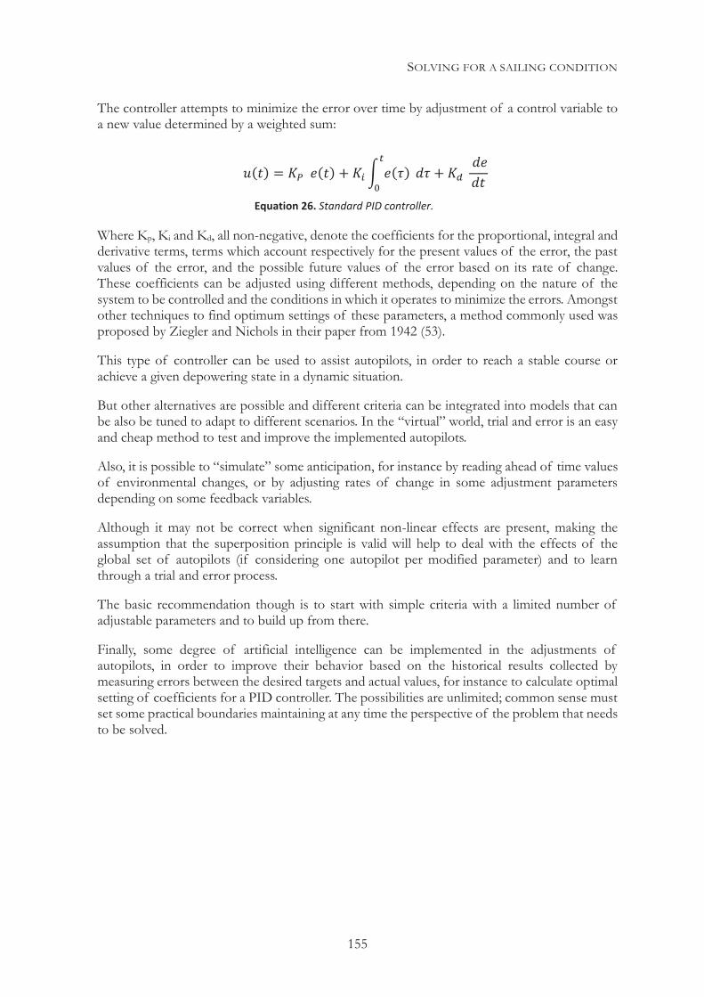
SOLVING FOR A SAILING CONDITION
155
The controller attempts to minimize the error over time by adjustment of a control variable to a new value determined by a weighted sum:
Where Kp, Ki and Kd, all non-negative, denote the coefficients for the proportional, integral and derivative terms, terms which account respectively for the present values of the error, the past values of the error, and the possible future values of the error based on its rate of change. These coefficients can be adjusted using different methods, depending on the nature of the system to be controlled and the conditions in which it operates to minimize the errors. Amongst other techniques to find optimum settings of these parameters, a method commonly used was proposed by Ziegler and Nichols in their paper from 1942 (53).
This type of controller can be used to assist autopilots, in order to reach a stable course or achieve a given depowering state in a dynamic situation.
But other alternatives are possible and different criteria can be integrated into models that can be also be tuned to adapt to different scenarios. In the “virtual” world, trial and error is an easy and cheap method to test and improve the implemented autopilots.
Also, it is possible to “simulate” some anticipation, for instance by reading ahead of time values of environmental changes, or by adjusting rates of change in some adjustment parameters depending on some feedback variables.
Although it may not be correct when significant non-linear effects are present, making the assumption that the superposition principle is valid will help to deal with the effects of the global set of autopilots (if considering one autopilot per modified parameter) and to learn through a trial and error process.
The basic recommendation though is to start with simple criteria with a limited number of adjustable parameters and to build up from there.
Finally, some degree of artificial intelligence can be implemented in the adjustments of autopilots, in order to improve their behavior based on the historical results collected by measuring errors between the desired targets and actual values, for instance to calculate optimal setting of coefficients for a PID controller. The possibilities are unlimited; common sense must set some practical boundaries maintaining at any time the perspective of the problem that needs to be solved.
Equation 26. Standard PID controller.

SOLVING FOR A SAILING CONDITION
156
This page intentionally left blank
DESCRIPTION OF THE TOOL. PASIM
157
7| DESCRIPTION OF THE TOOL. PASIM The previous Chapters have been dedicated to discussing the key components required to perform different types of performance predictions for a sailing yacht in a general way.
The next task consists in putting together those components in a working tool, in this case a computer program. This tool will need to manage the input and output of data, perform calculations using that data and provide a user interface to control all those tasks in order to provide means for an either interactive or automated execution.
This involves defining the basic program architecture, specifying and programming the different components, and defining how they interact with each other and with the “outside word”, whether that represents a human user or other computer programs.
This Chapter intends to describe those aspects and explain the process followed to reach the current configuration of the tool designed with that purpose: PASim (acronym of Performance Analysis and Simulation).
PROGRAM MODULES/COMPONENTS PASim comprises a variety of different elements integrated in a single piece of software. Some of those elements are fundamental components, required to carry out a performance analysis, but some others are auxiliary tools to assist the user in the process of managing and evaluating input data and final results, as well as analyzing the solution process. How those elements are integrated will be discussed later but, at this point, it is necessary to make a basic description of the different components included, starting with a definition of what is PASim expected to deliver.
7.1.1 THE TASKS TO PERFORM
Before describing the components, we will start by making a list of the tasks that PASim is expected to perform, as a simplified specification, in order to define the features that need to be incorporated and integrated via the different modules. Those tasks include the ability to:
Interact with the user via a graphic interface.
Interact with other programs.
Provide the possibility of an automated execution, managed either by the user or by an external mechanism of control.
Read and write files locally.
Import, process and modify (in a basic limited way) geometry definitions.
Perform extended hydrostatic calculations, including stability and calculation of custom effective parameters and coefficients.
DESCRIPTION OF THE TOOL. PASIM
158
Provide a wide range of models for the calculation of forces with tools to select alternative configurations, and facilitate implementing custom user defined models.
Provide a wide range of parameters available for manual adjustment and/or as optimization variables.
Provide the possibility to implement constraints over a range of different variables or functions of them.
Provide the ability to consider the six degrees of freedom when calculating equilibrium with the possibility of applying constraints on an arbitrary number of them.
Provide different implementations of solvers to calculate steady-state equilibrium or optimization with full control of the user over the solving parameters.
Provide a solving scheme for time-domain analyses with full control of the user over the solving parameters. This process will integrate the use of basic autopilots and will be open to implement more complex alternatives.
Provide the possibility of performing interactive calculations.
Provide a tool to analyze/evaluate data including the ability to generate plots based on it.
These features are expressed in very general terms, but they permit to make a broad definition of the main modules/components that need to be included in PASim, and that will be discussed in more detail in the next section.
7.1.2 THE MAIN PROGRAM MODULES/COMPONENTS
To fulfill the requirements described above, PASim includes a number of components that have been developed in a structured way, in order to facilitate their update/replacement. The program architecture will also be briefly discussed in the next sections, but the following paragraphs are limited to describing the main individual components along with of some of their capabilities.
Graphical user interface
After some doubts between using a unified user interface or an alternative in which each module would have its corresponding part of the interface, the final implementation has a single graphical user interface as a separate layer that communicates with the different modules, in those cases where they require an interaction with the user.
Fully coded in Microsoft Visual Studio VB.NET, PASim’s .NET managed code follows the usual structure and conventions of modern programs running in Microsoft Windows. That includes standard menus and shortcuts, dialogs, and the use of the Windows clipboard for cutting, copying and pasting in the program itself and to/from other programs. The user interface provides the direct connection with the user to perform all the tasks that require interaction and visualization of data or calculations, also allowing to directly setting the preferences for the different modules and, in general, any required adjustments.
The user interface also provides the main route to deliver messages to the user, whether they are regarding status, errors or results, depending on the options selected by the user. However,
DESCRIPTION OF THE TOOL. PASIM
159
sometimes direct warning and input simple dialogs are directly generated by the code in the modules where most of the error management is included.
Geometry management modules
There are three modules for the management and definition of geometries and they all permit definitions with at least two levels of detail regarding the definition. Obviously, the simplest option would limit the models that PASim can use, to those only requiring the most reduced set of parameters.
The first module permits to define the sail plan geometry as well as the inventory of available sails. These sails can be grouped in specific “sail sets” to be used in the calculations. Each one of these sets also has associated parameters that describe them, along with the rules regarding their variations and use.
The second module permits to define specific types of appendages, as well as a generic type, once again along with the rules regarding any possible adjustment they may be capable of. The possible types of appendages include from simple lifting surfaces such as keels or rudders, to bodies such as bulbs, including others like canting keels or lifting boards.
The third module is dedicated to the definition of the geometry of the hull (or hulls). For convenience and compatibility reasons, it uses a structure similar to the offsets file format implemented in the IMS. This module includes a graphic offsets editor that permits to review or modify points, as well as to interpolate additional stations. As the IMS offsets files include appendages, this module permits to clip them off from the hull itself, with the possibility of extracting basic measurements from the appendages, to be used as their basic definition, in case no better information is available. However, the recommended practice is to input the detailed definition of the appendages in their corresponding module, separate from the hull definition.
The hull can be moved or rotated in order to match a given flotation or any other arbitrary position. It can also be scaled and/or modified in different ways.
In addition, a simple tool is provided to import hulls defined as a NURBS surface, producing from the surface an offset file for a given set of section positions. This is a necessary step, given that the offsets format is used by the hydrostatic module to read the geometry and perform calculations.
Weights management module
This component permits to define the weights and inertias of the yacht, including movable weights and ballast tanks. It also allows to define whichever weight movements may be caused by other adjustments, for instance in the appendages or the sail plan. Although this module provides an independent management of weights, it is linked to the other geometry definition modules that include the specification of weights.
Windage management module
In an analogous way to weights, this component permits to define the windage parameters of different components of the yacht, including rig, hull, deck and crew. Although this module provides an independent management of windage, it is linked to the other geometry definition modules that include the specification of data related to windage.
DESCRIPTION OF THE TOOL. PASIM
160
Hydrostatic calculations module
This module is responsible for all the hydrostatic calculations performed using the hull and appendages geometries. These calculations take place on demand, either by the user, a requested specific calculation or by the mathematical models that may require a calculation for a specific condition under analysis. Displacement and center of gravity can either be supplied as values, or via the definition of a given set of freeboards at specific stations. In this last case, a value of VCG needs to be supplied by the user in order to perform stability calculations.
The manager or the specific calculation (the user or a calculation process) may require the use of different hydrostatic parameters. A wide range of parameters and coefficients are calculated by this module, ranging from physical traditional parameters to specific custom coefficients or effective values, which, for instance, include the effective parameters defined in the IMS.
The basic calculation provides all the relevant values for whichever flotation is analyzed and, based on them, more complex calculations can be performed. The structure of the module and calculation method is similar to the “Lines Processing Program” (LPP) included in the IMS, but with added flexibility, as well as additional calculated parameters and conditions.
File input/output module
File input and output routines are placed in a separate module with its own input/output error management. They are called from the other components of the main program whenever this is required.
This module allows to read and write all the files including data used by PASim, as well as to import a number of different formats for compatibility purposes. This includes some standard ASCII files with a basic description of their content in the first rows, so data can be easily prepared to facilitate its use in PASim.
But for managing its own data, PASim uses XML based files. Although this is not a format characterized for its speed in terms of reading/writing its file, it provides a flexibility that compensates this handicap, especially considering the limited time that PASim expends accessing files. The XML format also permits to better manage the inclusion of new data in the same type of files, without requiring altering their structure; therefore it is the recommended file format to interact with PASim. Additionally, although its use is not advised, PASim provides the possibility of using ASCII files to manage an asynchronous automated execution of the program.
Automation module
Given the object-oriented nature of PASim (that will be briefly described in section 7.2), there are a number of public methods available to perform the relevant actions necessary for an automated execution. This module provides an interface to use these methods in a simple way.
The automation module is a simple parser that translates simple commands into the specific methods for the sequential execution of the code. This module also allows controlling aspects such as the input and output of data, the definition of a specific problem, the pre and post-process of data and the execution of calculations. It includes simple decision structures.
Calculations module
This module groups all the available models for the calculation of forces and moments, including whichever pre-processing may be necessary. While the front end to interact with the
DESCRIPTION OF THE TOOL. PASIM
161
user for the selection and configuration of the models is in the graphic interface, this is the module where calculations are actually performed.
Although they are included in a separate library, there is a repository of auxiliary mathematical routines, available to any of the PASim components.
Data Assessment module
This module allows the display and analysis of data inside PASim. Its main purpose is the evaluation of different interpolation techniques and the quality of the data, including its first derivatives.
It also makes use of a library of interpolation routines from the repository of auxiliary mathematical routines, and includes a graphical representation of the data with the possibility to select different sectional cuts of multidimensional data.
This module is also intended to prepare experimental and numerical data for their use in the calculations with the best possible data fit, providing a measure of the possible errors in which the interpolation incurs and, as stated before, of derivatives that can affect the solvers’ performance.
Solvers
Solvers are grouped together in a specific module providing a coherent similar call for the different alternatives, mainly for the stationary-state calculations and optimization, although the ODE solvers are included here as well.
The main idea is to separate these algorithms from the rest of the program, providing for the solvers the necessary callback functions to interface with the calculations module. Each solver also has adjustable preferences. These include a number of operational settings that range from the step size control to the procedure to estimate derivatives, or even the possibility of providing pre-calculated derivatives directly to the solver.
Reports
After a successful calculation, PASim provides the possibility of generating specific reports as a post-processed output of the results, which can be customized, depending on the objective. These results can be accessed in the screen, as well as exported as XML or ASCII files.
The content of the reports can range from the result of a simple isolated hydrostatic calculation to the output of a full VPP analysis. This may include information such as hydrostatic calculations, recollection of the models used, results of pre-processing, solver statistics and full detailed results for each calculation point (including or not a detailed breakdown of the forces).
7.1.3 ALGORITHMS IMPLEMENTATION
In the previous chapters, a number of algorithms of very different nature have been discussed, ranging from those intended for the calculation of forces to auxiliary mathematical tools to manage data or solve equilibrium. The following list provides a non-exhaustive list of relevant algorithms implemented in PASim to perform several different tasks:
DESCRIPTION OF THE TOOL. PASIM
162
Models for the calculations of Forces
Delft models for the calculation of forces, including residuary and viscous drag for hull and appendages, as well as for the calculation of resistance added in waves.
Viscous drag calculations for laminar and turbulent flows.
Form factor estimates for the calculation of viscous drag in lifting surfaces and immersed bodies.
ITTC 57 and Shoenherr friction lines for viscous drag calculations.
IMS hull residuary drag calculation (models from 1987 to 2000).
Classical IMS sail model with different variations and adjustments.
A generic sail model scheme for data of experimental or numerical origin.
Lifting line theory calculations for lifting surfaces in general.
Data fitting meta-models for experimental and numerical results.
Hydrostatics and stability direct calculations based on the defined geometries and weights.
Models for representation and interpolation of data
Polynomial interpolation of different orders.
Cubic spline interpolation with some limited control for extrapolation.
NURBS surfaces.
Fairing splines.
Solving/Optimization algorithms
SOLVER (54). A general-purpose commercial solver for constrained optimization produced by Frontline Inc., which allows a high degree of customization, providing different internal algorithms for linear and non-linear problems. This is a particularly robust optimizer with a high rate or convergence. The implemented solver is a stand-alone version (presented as a compiled “DLL” file) of the solver tool included in Microsoft Excel. For its integration within other programs, it provides a callback procedure to allow the solver component to call the routine for the evaluation of forces in the host program (PASim), in order to allow the calculation of the values of constraints, objective function and derivatives. This way, while maintaining a “black-box” style, the solver provides the necessary interface with the mathematical models. In other words, it provides a connection between the optimization engine and the calculation of forces and moments required by the process.
LINDO (55). A general-purpose commercial solver for constrained optimization produced by Lindo Systems Inc., which allows a high degree of customization. It provides internal algorithms for linear and non-linear problems. Its integration with PASim is done in a similar way to the integration of the Frontline Solver, through a “DLL” compilation, and using a “black-box” style interface and a callback procedure to evaluate constraints, objective function and derivatives.
NLPQLP (56) (57). An optimization code for solving constrained nonlinear optimization problems where all functions are continuously differentiable, developed by Prof. Klaus
DESCRIPTION OF THE TOOL. PASIM
163
Schittkowski from the University of Bayreuth (Germany). It is a powerful, robust and stable solution (this code, ported to VB.NET, is implemented for the research purposes of this investigation under the restrictions of the license provided by the author).
COBYLA (48). An optimization algorithm for non-linear problems developed by M.J.D. Powell for use when no derivatives are available.
CONMIN (58). An algorithm developed by G.N. Vanderplaats for constrained function minimization.
Spider (50). A method for numerical constrained optimization developed by Ronald N. Perry, based on the Nelder-Mead Simplex method, with the use of a new method to manage constraints. This method is especially well suited for situations when the optimal solutions are actively limited by the constraints.
CONMAX (51). An ODE-based approach to non-linearly constrained problems that for each iteration solves approximately a system of nonlinear ordinary differential equations to get a direction for the line search. Although slower than other methods, this algorithm provides a robust solution for cases where other methods fail to converge.
The Newton-Raphson method for systems of non-linear equations.
The Runge-Kutta fourth order, Midpoint and Euler methods for ordinary differential equations (ODE).
Control algorithms
A proportional integral derivative (PID) controller (52) with integral windup protection for assistance to autopilots.
PROGRAM ARCHITECTURE After a general description of the different modules included in PASim, it is necessary to briefly discuss the structure of the program, providing a general vision about how all the modules fit to form PASim.
7.2.1 SOME HISTORY
PASim first antecessor started as a very simple tool, based on three nested iterative schemes to perform a calculation of equilibrium for forces in the X-axis and moments around it, with a depowering variable (reef) to be optimized as a part of the process.
It was programmed initially in Visual Basic 3.0 and soon progressed to incorporate most of the IMS models from the available source code, until a first working version, which included a basic graphical user interface, was ready. This version already allowed the use of towing tank data for its analysis and evaluation.
Different models were incorporated over the years until the program turned into PAP, a tool programmed in Microsoft Visual Studio using VB.NET as the core language. PAP had a strictly procedural architecture and included most of the modules required for a general performance
DESCRIPTION OF THE TOOL. PASIM
164
analysis in a somewhat modular way, but with a significant interdependency between the user interface and the calculation modules, as well as between the modules themselves.
After the 32nd America’s Cup in 2007, it became evident that a new evolutionary step was necessary, and this fact, along with the need to deal with an increasing variety of yacht types and calculations, pointed in the direction of a more general, flexible and modern approach. That need set the basic concepts of what PASim should incorporate along with its basic structure, to be investigated and developed over the following years in order to facilitate its adaptation to a whole range of new uses.
7.2.2 OBJECT-ORIENTED VS. PROCEDURAL ARCHITECTURE
PASim is a departure from PAP, and although there was never any intention to abandon all the work put in place in the original code, it was necessary to start from a new simpler structure. This was motivated by the need to overcome some of the inherent limitations of an older code and facilitate communication, both internal (between modules) and external (with other programs). It also required a cleaner and simpler separation between the different components of the program.
After some careful evaluation, it became evident that a more object-oriented structure would better serve the new requirements, starting at the same time from a simpler and more organized code than PAP, which throughout its development had been turning into a complicated mix of routines.
The object-oriented approach became especially convenient for that data that could be grouped in a specific class, in which specific methods could also be defined to operate with the data inside the class.
However, a number of operations with the properties of the objects need to happen outside of the class, with functions depending simultaneously on properties from a number of different objects. Because of this, completely avoiding a procedural structure became very difficult. That was the reason to adopt a hybrid architecture, trying at all times to preserve a structure as modular as possible.
Some of the objects have overlapped linked properties to be directly used inside the respective classes, but external routines also operate reading the object properties for their process. With all those considerations, this approach started to be implemented, identifying the main classes that would constitute the program:
Graphical User Interface (GUI). Defined as a collection of objects, which include some external components related to the interface, such as TeeChart and iGrid.
Execution interface. Placed underneath the GUI, constitutes the main class to manage the program, either communicating with the user interface or providing the interface for automated execution.
Yacht. Collection of other objects (Hull, Sail plan, Appendages (also a collection of other objects by itself), weights, etc.) that contains all the properties of the yacht to be analyzed, as well as a number of methods for their manipulation.
DESCRIPTION OF THE TOOL. PASIM
165
Calculation: Constituted by a definition of the constraints, variables, solving procedure etc.; in summary, it comprises all the properties that characterize the type of calculation to be performed and the method/s used.
Solution: Defined as the output of a calculation that may comprise:
One calculated point with references to the yacht analyzed, balance of forces, settings, models used etc.
A collection of calculated points defining a steady-state solution and/or the process towards it.
A collection of calculated points defining a time-domain analysis.
7.2.3 .NET EXTERNAL COMPONENTS
Within the .NET managed code approach, it is possible to use a number of objects to build the graphic interface without requiring to manually generate all the necessary code. In addition, there are also commercial and open source components, available for many specific tasks. This, again, reduces the amount of coding required for general tasks and provides high quality solutions, which can be incorporated in the program. For those reasons, there are two main components that were implemented in PASim in the construction of the visual user interface.
TeeChart (59) was the choice for representing data graphically because of its ability to display data in a wide range of different types of plots. TeeChart provides a simple interface that allows the programmer to use a large number of resources to display data, manipulate the plots, zoom, perform statistical analyses etc. It also facilitates a richer interaction with the user.
iGrid (60) is used to provide a spreadsheet-like grid that facilitates viewing, sorting, inputting and editing data in a familiar and consistent way. It also has additional displaying, printing, and formatting capabilities over the grid component included in Visual Studio. That is the reason why it was adopted as the choice for the visual tabulated data interface with the user.
INTERFACING Some of the reasons for the new structure of PASim were related to facilitating the automation of the execution of the program and the interface with external data and other problems. This way, the integration as a part of multi-component projects is significantly facilitated.
As a response to those requirements, two decisions were taken: to use XML as the basic file format to store input data, preferences, output data etc., and to make some of the objects public and accessible to external programs, which would then be able to control PASim in a seamless way.
7.3.1 XML FORMAT
Full compatibility with older ASCII files from PAP have been preserved and specific data input ASCII formats are suggested (easier to create for users not familiar with XML, for instance, as the output of a spreadsheet). However, the recommendation for all the main files managed by PASim is to use XML as a simple, flexible and organized way to store data.
DESCRIPTION OF THE TOOL. PASIM
166
XML (Extensible Markup Language) is a markup language (a system for annotating a document in a way that is syntactically distinguishable from the text). Its purpose is to define a set of rules for encoding documents in a format, which is both human-readable and machine-readable. The capabilities of XML significantly exceed the small fraction of its definition that is implemented in PASim, with hundreds of document formats based today on the syntax of this language.
Although XML based files are by no means databases, they provide a flexible technology for storing and porting limited amounts of data and facilitate its access from computer programs.
XML base files have a nested tag structure that normally requires reading the complete file in order to access one specific stored value and, as it has been mentioned before, they are not an efficient alternative in terms of writing or reading speed for large amounts of data, also generating relatively large files. However, that is not the normal situation with the type of data under consideration in a VPP, where flexibility and readability are more relevant than reading/writing speed. One exception would be the case of large time-domain analysis, where the use of an actual database format becomes a more logical choice given the large amount of generated data.
Another advantage of XML files for the exchange and representation of data is that generic code can read or write them, as well as display its content already formatted (if formatting instructions are present), without a prior knowledge of the content itself. This facilitates compatibility and portability of the data included in the file without having the data itself altered by any additional formatting elements that may be included.
All those reasons, along with the available resources to conveniently organize the data inside the files (especially when the data is represented by objects inside the application) made XML the choice for storing and transferring data in PASim.
7.3.2 INTERFACING WITH EXTERNAL PROGRAMS
Although PASim is structured in different modules, some of them compiled as Dynamic Link Libraries (DLL), the main program is defined as well as a DLL, with some of the classes required to run automated execution publicly accessible to other programs that may call and drive the main PASim DLL.
This facilitates the use of PASim as a component of global projects that may require VPP calculations or even access to parts of PASim, for instance to perform a calculation of forces or a hydrostatic analysis.
The main condition for other programs to facilitate this communication is to be compiled as .NET managed code. No requirements are made regarding the language in which they are programmed. The use of managed code is not a strict requirement, but it significantly facilitates the communication process. An alternative sometimes used is creating a small interface program compiled as .NET managed code called by the driving program.
Alternatively, it is possible to run the executable launcher of PASim with arguments and/or automation files (the arguments being much more limited than the possible actions through the DLL call). Although this makes more difficult to run PASim in an interactive synchronous way, it is still possible to verify whether the tasks requested to PASim have been finalized and, while it is by far a less elegant solution, it allows virtually any program to execute PASim.
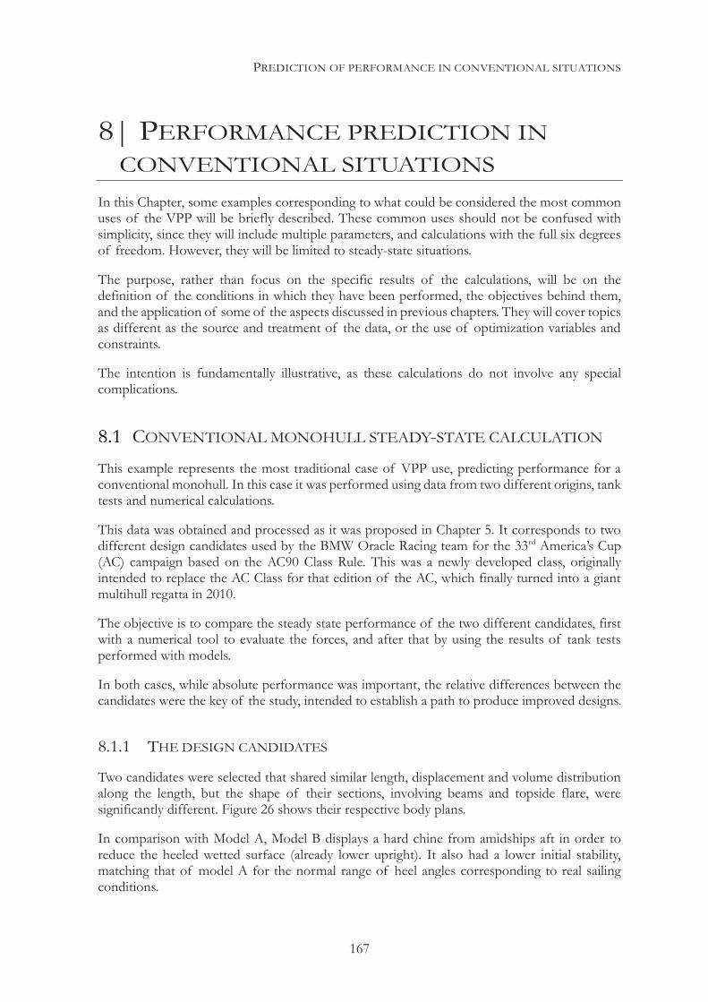
PREDICTION OF PERFORMANCE IN CONVENTIONAL SITUATIONS
167
8| PERFORMANCE PREDICTION IN CONVENTIONAL SITUATIONS
In this Chapter, some examples corresponding to what could be considered the most common uses of the VPP will be briefly described. These common uses should not be confused with simplicity, since they will include multiple parameters, and calculations with the full six degrees of freedom. However, they will be limited to steady-state situations.
The purpose, rather than focus on the specific results of the calculations, will be on the definition of the conditions in which they have been performed, the objectives behind them, and the application of some of the aspects discussed in previous chapters. They will cover topics as different as the source and treatment of the data, or the use of optimization variables and constraints.
The intention is fundamentally illustrative, as these calculations do not involve any special complications.
CONVENTIONAL MONOHULL STEADY-STATE CALCULATION This example represents the most traditional case of VPP use, predicting performance for a conventional monohull. In this case it was performed using data from two different origins, tank tests and numerical calculations.
This data was obtained and processed as it was proposed in Chapter 5. It corresponds to two different design candidates used by the BMW Oracle Racing team for the 33rd America’s Cup (AC) campaign based on the AC90 Class Rule. This was a newly developed class, originally intended to replace the AC Class for that edition of the AC, which finally turned into a giant multihull regatta in 2010.
The objective is to compare the steady state performance of the two different candidates, first with a numerical tool to evaluate the forces, and after that by using the results of tank tests performed with models.
In both cases, while absolute performance was important, the relative differences between the candidates were the key of the study, intended to establish a path to produce improved designs.
8.1.1 THE DESIGN CANDIDATES
Two candidates were selected that shared similar length, displacement and volume distribution along the length, but the shape of their sections, involving beams and topside flare, were significantly different. Figure 26 shows their respective body plans.
In comparison with Model A, Model B displays a hard chine from amidships aft in order to reduce the heeled wetted surface (already lower upright). It also had a lower initial stability, matching that of model A for the normal range of heel angles corresponding to real sailing conditions.
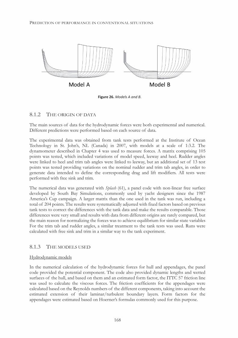
PREDICTION OF PERFORMANCE IN CONVENTIONAL SITUATIONS
168
8.1.2 THE ORIGIN OF DATA
The main sources of data for the hydrodynamic forces were both experimental and numerical. Different predictions were performed based on each source of data.
The experimental data was obtained from tank tests performed at the Institute of Ocean Technology in St. John’s, NL (Canada) in 2007, with models at a scale of 1:3.2. The dynamometer described in Chapter 4 was used to measure forces. A matrix comprising 105 points was tested, which included variations of model speed, leeway and heel. Rudder angles were linked to heel and trim tab angles were linked to leeway, but an additional set of 13 test points was tested providing variations on the nominal rudder and trim tab angles, in order to generate data intended to define the corresponding drag and lift modifiers. All tests were performed with free sink and trim.
The numerical data was generated with Splash (61), a panel code with non-linear free surface developed by South Bay Simulations, commonly used by yacht designers since the 1987 America’s Cup campaign. A larger matrix than the one used in the tank was run, including a total of 204 points. The results were systematically adjusted with fixed factors based on previous tank tests to correct the differences with the tank data and make the results comparable. Those differences were very small and results with data from different origins are rarely compared, but the main reason for normalizing the forces was to achieve equilibrium for similar state variables For the trim tab and rudder angles, a similar treatment to the tank tests was used. Runs were calculated with free sink and trim in a similar way to the tank experiment.
8.1.3 THE MODELS USED
Hydrodynamic models
In the numerical calculation of the hydrodynamic forces for hull and appendages, the panel code provided the potential component. The code also provided dynamic lengths and wetted surfaces of the hull, and based on them and an estimated form factor, the ITTC 57 friction line was used to calculate the viscous forces. The friction coefficients for the appendages were calculated based on the Reynolds numbers of the different components, taking into account the estimated extension of their laminar/turbulent boundary layers. Form factors for the appendages were estimated based on Hoerner’s formulas commonly used for this purpose.
Figure 26. Models A and B.
PREDICTION OF PERFORMANCE IN CONVENTIONAL SITUATIONS
169
For the expansion of the tank data to full scale, the same viscous approach described above was used along with a calculated form factor for the hull, based on low-speed bare-hull runs and the Prohaska method.
The smaller set of data from the tank was expanded creating additional “virtual” data based on the existing data, taking as a reference the numerical results. Cubic spline interpolation was used on the full final expanded matrices for both numerical and experimental data (and corrected in the case of the numerical data), to obtain intermediate values for the calculations.
The calculations were performed in flat water. No added resistance in waves was considered.
Aerodynamic models
For the calculation of the sail forces, a tweaked version of the IMS sail model was used. This version implemented a modified reef parameter that reduced the sail area by assuming smaller headsails, and a flat parameter, which included a twist effect linked to the degree of flat.
The IMS model for parasitic drag was used to estimate this force component for both the sail plan and the exposed part of the hull, with a standard wind gradient calculation adapted to the heights of the different elements (to estimate apparent wind speeds and angles).
Alternative runs in the VPP were tested with a model built from a matrix run in the SK2V code. This model provided forces as a function of the wind and three adjustment parameters, flat, twist (directly related to mainsheet tension) and traveler position, reproducing the normal trimming procedures and selections of sails. However, this model used headsails with different sizes instead of a continuous variation, which added some level of uncertainty when comparing hull designs through a range of wind speeds. The results were comparable for the range of use of each sail, which was kept the same for both yachts.
Stability
Stability calculations were performed for each hull geometry as part of the pre-process, using the same center of gravity, free trim and an estimated sail-induced pitch moment.
8.1.4 THE CALCULATION
For the calculation of the steady state performance, the track axes were used. Equilibrium was forced only in two degrees of freedom: forces along the X-axis (drag vs. driving force) and moments around the same X-axis (heeling force vs. righting moment). Forces in the Y-axis were also assumed balanced by matching the hydrodynamic force with the projected component of the generated aerodynamic force in this axis, prior to the calculation of its corresponding hydrodynamic induced drag (thus, equilibrium was also implicitly forced in the Y-axis).
Regarding vertical forces and pitch moments, equilibrium was assumed with no further analysis. Given that the heave and pitch equilibrium was reached for each test point when performing the tank tests or numerical analyses (by using free sink and trim), it was expected to happen as well for the converged VPP situations. This is a common assumption that guarantees small errors in the equilibrium of forces for those degrees of freedom, not explicitly considered.
Given that the purpose of the study was to compare hull shapes, it was assumed that the sail plan would be positioned in a longitudinal position that would guarantee equilibrium in the yaw
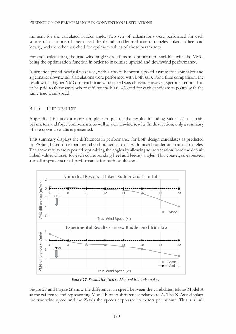
PREDICTION OF PERFORMANCE IN CONVENTIONAL SITUATIONS
170
moment for the calculated rudder angle. Two sets of calculations were performed for each source of data: one of them used the default rudder and trim tab angles linked to heel and leeway, and the other searched for optimum values of those parameters.
For each calculation, the true wind angle was left as an optimization variable, with the VMG being the optimization function in order to maximize upwind and downwind performance.
A generic upwind headsail was used, with a choice between a poled asymmetric spinnaker and a gennaker downwind. Calculations were performed with both sails. For a final comparison, the result with a higher VMG for each true wind speed was chosen. However, special attention had to be paid to those cases where different sails are selected for each candidate in points with the same true wind speed.
8.1.5 THE RESULTS
Appendix I includes a more complete output of the results, including values of the main parameters and force components, as well as a downwind results. In this section, only a summary of the upwind results is presented.
This summary displays the differences in performance for both design candidates as predicted by PASim, based on experimental and numerical data, with linked rudder and trim tab angles. The same results are repeated, optimizing the angles by allowing some variation from the default linked values chosen for each corresponding heel and leeway angles. This creates, as expected, a small improvement of performance for both candidates.
Figure 27 and Figure 28 show the differences in speed between the candidates, taking Model A as the reference and representing Model B by its differences relative to A. The X-Axis displays the true wind speed and the Z-axis the speeds expressed in meters per minute. This is a unit
Figure 27. Results for fixed rudder and trim tab angles.

PREDICTION OF PERFORMANCE IN CONVENTIONAL SITUATIONS
171
commonly used amongst racing sailors, since it provides a measure of performance that can be easily related to on board observations when two yachts are sailing close to each other. The type of plot selected to display these results was used for the first time by F. Villalonga with the “Bravo España” team during the 30th America’s Cup campaign, and has become a common standard.
It is easy to confirm that the predictions with data from different origins display comparable trends. However, although small, there are some clearly visible differences between them.
When performing the calculations with optimized rudder and trim tab angle the trends are similar. This could be expected, given the relatively small differences between the two designs, limited to the hull shape (and derived effects from that, such as changes in stability).
MULTIHULL STEADY-STATE CALCULATION This example intends to illustrate steady-state calculations with six degrees of freedom, forcing additional constraints and studying different sailing modes as described in Chapter 6. This was achieved using a catamaran and a range of models to estimate forces from different origins.
As discussed briefly before, multihulls are a good example of force balance, multi-parametric optimization and full use of six degrees of freedom in the definition of a steady-state equilibrium. In this example, a catamaran was used to calculate solutions, showing:
The use of multiple optimization parameters.
Equilibrium in six degrees of freedom.
Figure 28. Results for optimized rudder and trim tab angles.
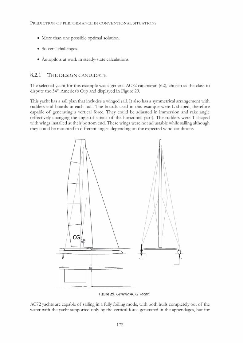
PREDICTION OF PERFORMANCE IN CONVENTIONAL SITUATIONS
172
More than one possible optimal solution.
Solvers’ challenges.
Autopilots at work in steady-state calculations.
8.2.1 THE DESIGN CANDIDATE
The selected yacht for this example was a generic AC72 catamaran (62), chosen as the class to dispute the 34th America’s Cup and displayed in Figure 29.
This yacht has a sail plan that includes a winged sail. It also has a symmetrical arrangement with rudders and boards in each hull. The boards used in this example were L-shaped, therefore capable of generating a vertical force. They could be adjusted in immersion and rake angle (effectively changing the angle of attack of the horizontal part). The rudders were T-shaped with wings installed at their bottom end. These wings were not adjustable while sailing although they could be mounted in different angles depending on the expected wind conditions.
AC72 yachts are capable of sailing in a fully foiling mode, with both hulls completely out of the water with the yacht supported only by the vertical force generated in the appendages, but for
Figure 29. Generic AC72 Yacht.
PREDICTION OF PERFORMANCE IN CONVENTIONAL SITUATIONS
173
this example, the analysis was limited to the light air situations in which foiling does not normally happen.
The center of gravity was positioned approximately aft of the boards, permitting to act on the pitch moment by using vertical force of the boards in order to counteract the pitch moment induced by the driving force generated in the sail plan.
The following adjustments were available to achieve equilibrium and optimize performance:
Depowering parameters flat and twist for the sail plan, affecting the generated aerodynamic forces and vertical center of effort.
Leeward board immersion and rake angle (in this example, those parameters were left at a fixed value, considered adequate for the range of wind conditions in which the calculations were performed).
Rudder angle, affecting the yaw equilibrium.
This permitted sufficient control over the yacht to guarantee that steady-state solutions could be achieved for a reasonable range of wind speeds and angles.
8.2.2 THE MODELS USED
Hydrodynamic models
For the hull forces, a generic AC72 hull was designed and run through a panel code (Splash) with fixed sink and trim, for a matrix with variations of speed, pitch angle and sinkage.
Only one hull was analyzed, after confirming that given the hulls separation and geometry, no significant interference between them would happen at the speeds for which both hulls would be inside the water.
Forces were measured and moments computed from the results. A multidimensional spline interpolation was used on the final set of force data, which included additional “virtual” points to extend the parametric space in a fair way.
The rudder and board forces were calculated using analytical models, taking into consideration their geometries, positions, and the incoming flows. The bi-dimensional characteristics of the rudder and board sections were calculated with Xfoil (42) in order to estimate the drag for the operating lift coefficients.
Aerodynamic models
The sail plan model was based on a lifting line calculation, with the bi-dimensional characteristics taken from multi-element foil data and applying limitations to the possible span-wise variation of the lift coefficients.
The depowering parameters were implemented in a similar way to the IMS corresponding ones, with flat and twist effectively affecting the generated lift and vertical center of effort (as well as their influence on drag).
PREDICTION OF PERFORMANCE IN CONVENTIONAL SITUATIONS
174
Given the high apparent wind speeds in which multihulls sail, parasitic drag is particularly relevant in this type of yacht. Calculations were performed with estimated drag coefficients for different components (limited in this case to the main contributors: rig, windward and leeward hulls, and crew). Additionally, for each one of the windage elements, the apparent wind was calculated by solving the wind triangle for their corresponding heights, using a standard wind gradient model.
Hydrostatic model
No previous stability calculation was performed. Instead, hydrostatic forces included in the Splash results (which include a “Froude-zero” result, comprising only static forces) were used. Therefore, the hydrostatic forces were evaluated for each calculation point, along with all the other forces.
8.2.3 THE CALCULATION
For the calculation of the steady-state performance, the track axes were used. Equilibrium was forced in all six degrees of freedom with the corresponding constraints defined in Chapter 6. A true wind angle of 130 degrees was fixed for all wind speeds. The Frontline Solver was responsible for finding the optimal equilibrium points.
The most relevant issue during these calculations was due to the existence of two different sailing modes for some points, depending on whether the windward hull is partially immersed or completely above the water surface. Therefore, this phenomenon will be briefly discussed.
The hydrostatic forces for the windward hull decrease with immersion as the yacht starts to heel over, until the immersion reaches a zero value and the hull comes completely out of the water. In that case, we considered that the hull had a negative immersion, corresponding to the height at which the hull was flying.
This poses a problem to the solvers, since the first derivative of the hydrodynamic forces have an abrupt change, and from there it takes a constant value of zero. This situation has a negative influence on the solving process, and can lead to unexpected problems preventing convergence from happening. In order to avoid this, PASim mirrors the force values for negative values of immersion, creating some “fake” forces of opposite sign. This has the advantage that derivatives calculated beyond that point remain continuous and fair, without interfering with the optimizer solving process (even if they are calculated beyond variable bounds).
When a point is reached where the windward hull has no immersion, with constraints satisfied in all degrees of freedom (actually, the windward hull is constrained to not exceed a very small arbitrary flying height, which has an insignificant impact on drag), PASim stops the solver and an autopilot controlling the hull immersion constraint now fixes the height above water at 0.5 meters. Then the solution process restarts, using as initial values the ones when the process was interrupted. At that point the autopilot also sets the windward hull hydrodynamic forces to zero. The solver will then converge to a “flying situation”, which has been found feasible.
The convergence to a solution with the windward hull flying at 0.5 meters is a reasonable assumption, given that with slightly more heel, stability is reduced in a small amount, but the change is larger than the expected loss in aerodynamic heeling moment caused by that additional heel angle.
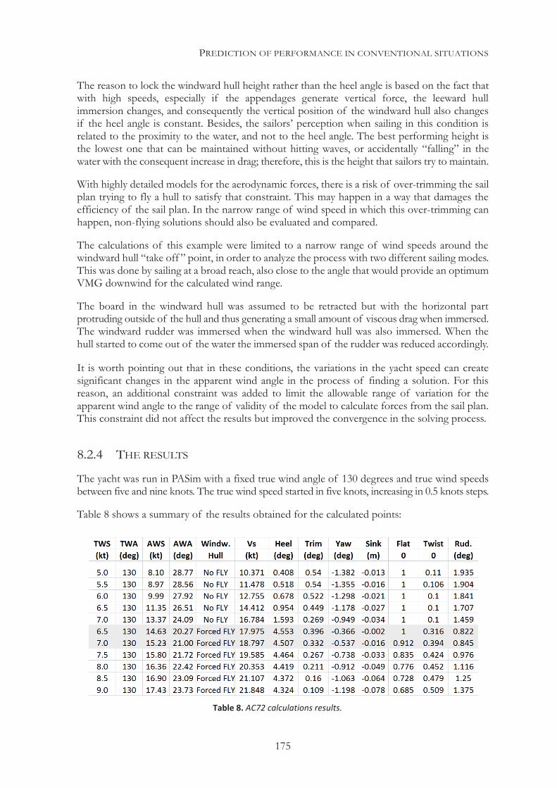
PREDICTION OF PERFORMANCE IN CONVENTIONAL SITUATIONS
175
The reason to lock the windward hull height rather than the heel angle is based on the fact that with high speeds, especially if the appendages generate vertical force, the leeward hull immersion changes, and consequently the vertical position of the windward hull also changes if the heel angle is constant. Besides, the sailors’ perception when sailing in this condition is related to the proximity to the water, and not to the heel angle. The best performing height is the lowest one that can be maintained without hitting waves, or accidentally “falling” in the water with the consequent increase in drag; therefore, this is the height that sailors try to maintain.
With highly detailed models for the aerodynamic forces, there is a risk of over-trimming the sail plan trying to fly a hull to satisfy that constraint. This may happen in a way that damages the efficiency of the sail plan. In the narrow range of wind speed in which this over-trimming can happen, non-flying solutions should also be evaluated and compared.
The calculations of this example were limited to a narrow range of wind speeds around the windward hull “take off ” point, in order to analyze the process with two different sailing modes. This was done by sailing at a broad reach, also close to the angle that would provide an optimum VMG downwind for the calculated wind range.
The board in the windward hull was assumed to be retracted but with the horizontal part protruding outside of the hull and thus generating a small amount of viscous drag when immersed. The windward rudder was immersed when the windward hull was also immersed. When the hull started to come out of the water the immersed span of the rudder was reduced accordingly.
It is worth pointing out that in these conditions, the variations in the yacht speed can create significant changes in the apparent wind angle in the process of finding a solution. For this reason, an additional constraint was added to limit the allowable range of variation for the apparent wind angle to the range of validity of the model to calculate forces from the sail plan. This constraint did not affect the results but improved the convergence in the solving process.
8.2.4 THE RESULTS
The yacht was run in PASim with a fixed true wind angle of 130 degrees and true wind speeds between five and nine knots. The true wind speed started in five knots, increasing in 0.5 knots steps.
Table 8 shows a summary of the results obtained for the calculated points:
Table 8. AC72 calculations results.
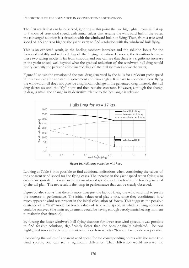
PREDICTION OF PERFORMANCE IN CONVENTIONAL SITUATIONS
176
The first result that can be observed, ignoring at this point the two highlighted rows, is that up to 7 knots of true wind speed, with initial values that assume the windward hull in the water, the converged solution is a situation with the windward hull not flying. Then, from a true wind speed of 7.5 knots or higher, the yacht starts to find a solution with the windward hull flying.
This is an expected result, as the heeling moment increases and the solution looks for the increased stability and reduced drag of the “flying” situation. However, the transition between these two sailing modes is far from smooth, and one can see that there is a significant increase in the yacht speed, well beyond what the gradual reduction of the windward hull drag would justify (actually the parasitic aerodynamic drag of the hull increases above the water).
Figure 30 shows the variation of the total drag generated by the hulls for a relevant yacht speed in this example (for constant displacement and trim angle). It is easy to appreciate how flying the windward hull does not provide a significant change in the generated drag. Instead, the hull drag decreases until the “fly” point and then remains constant. However, although the change in drag is small, the change in its derivative relative to the heel angle is relevant.
Looking at Table 8, it is possible to find additional indications when considering the values of the apparent wind speed for the flying cases. The increase in the yacht speed when flying, also creates an equivalent increase in the apparent wind speeds, and therefore in the forces generated by the sail plan. The net result is the jump in performance that can be clearly observed.
Figure 30 also shows that there is more than just the fact of flying the windward hull to justify the increase in performance. The initial values used play a role, since they conditioned how much apparent wind was present in the initial calculation of forces. This suggests the possible existence of a “fast” mode for lower values of true wind speed, in which a flying condition could be achieved (the main requirement would be having enough aerodynamic heeling moment to maintain that situation).
By forcing the faster windward hull-flying situation for lower true wind speeds, it was possible to find feasible solutions, significantly faster than the ones originally calculated. The two highlighted rows in Table 8 represent wind speeds in which a “forced” fast mode was possible.
Comparing the values of apparent wind speed for the corresponding points with the same true wind speeds, one can see a significant difference. That difference would increase the
Figure 30. Hulls drag variation with heel.
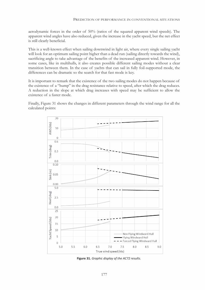
PREDICTION OF PERFORMANCE IN CONVENTIONAL SITUATIONS
177
aerodynamic forces in the order of 50% (ratios of the squared apparent wind speeds). The apparent wind angles have also reduced, given the increase in the yacht speed, but the net effect is still clearly beneficial.
This is a well-known effect when sailing downwind in light air, where every single sailing yacht will look for an optimum sailing point higher than a dead run (sailing directly towards the wind), sacrificing angle to take advantage of the benefits of the increased apparent wind. However, in some cases, like in multihulls, it also creates possible different sailing modes without a clear transition between them. In the case of yachts that can sail in fully foil-supported mode, the differences can be dramatic so the search for that fast mode is key.
It is important to remark that the existence of the two sailing modes do not happen because of the existence of a “hump” in the drag resistance relative to speed, after which the drag reduces. A reduction in the slope at which drag increases with speed may be sufficient to allow the existence of a faster mode.
Finally, Figure 31 shows the changes in different parameters through the wind range for all the calculated points:
Figure 31. Graphic display of the AC72 results.
PREDICTION OF PERFORMANCE IN CONVENTIONAL SITUATIONS
178
Some effects become more obvious looking at the graphic representation of the results:
The trim angle starts decreasing with the true wind speed (and yacht speed) due to the increase in the pitch moment created by the sail plan, in absence of changes in the boards rake (or setting the rudder wings at a different angle).
At lower speeds, the effects of starting to lift the windward hull dominate, producing an increase in sinkage. Once the windward hull starts flying, the effect of the vertical forces coming from the leeward board and the rudders’ wings starts to be more significant as speed increases, so the yacht starts to be more dynamically supported, reducing its sinkage.
In flying mode, as the yacht reduces its sinkage the heel angle starts to diminish. This is a direct consequence of the change in sinkage and the fact that the windward hull is forced to fly at a given height (in this case 0.5 meters clear of the water surface), so any change in sinkage requires an adjustment in the heel angle.
CHANGING ADJUSTMENTS IN SIX DEGREES OF FREEDOM The previous example already showed equilibrium happening in six degrees of freedom, but using a limited set of adjustments/parameters to be optimized, while the others were maintained at fixed positions. These parameters (sail depowering parameters and rudder angle) were enough (but required) to guarantee the existence of an equilibrium situation for the conditions of the calculation. However, there was little margin for their optimization.
In this section, the previous situation was extended to explore the additional control that could be added through different possible states of equilibrium in search for faster optima.
8.3.1 THE DESIGN CANDIDATE
For this example, the same AC72 yacht from section 8.2 was used. However, this time, additional adjustment parameters were available, subject to optimization within a specified range of variation:
The board had its immersion and rake angle adjustable (sailing choices).
The rudder wing angle was adjustable (sailing/design choice).
The longitudinal position of the center of gravity was adjustable (design choice).
This provided a different playground from the previous example, allowing the evaluation of the results of the interactions between the different adjustments.
8.3.2 THE MODELS USED
The same models as in the previous example were used for the calculation of forces. However, this time we took advantage of having the possibility to change different parameters that were left in a fixed value in the previous case.
PREDICTION OF PERFORMANCE IN CONVENTIONAL SITUATIONS
179
8.3.3 THE CALCULATION
The process for the calculation was also similar to before, but this time it was performed in an upwind situation with a true wind angle of 45 degrees through a range of stronger wind speeds, always with the windward hull flying, and still providing a variation in the yacht speeds to evaluate its effect on optimal parameters. The example with the effect of the angle of the rudder wings and optimum board rake also included some runs with the true wind angle of 130 degrees as in the previous example.
The windward hull flying height constraint was set again to 0.5 meters, and when changing the rake of the board at the higher speeds, the change in sinkage of the leeward hull showed effects on the achievable heel angle to a larger extent than when the board rake angle was fixed.
Some runs were performed optimizing only one of the new adjustments to see its effects, but some other times one parameter was fixed at different values and the rest optimized to evaluate their mutual effects. Sometimes, as it was anticipated in Chapter 6, a different combination of adjustments produced very similar performance, showing the interaction between the adjustments, but also raising a flag regarding how comparable the results were.
Finally, a global optimization was performed, leaving all the parameters free to change within given ranges, to observe the effect on the global performance.
It is interesting to note that the specific solver that we were using in this example (the Frontline Solver code) expends most of the time calculating forces when trying to reach the first point where all constraints are satisfied, and then, it progresses quickly to an optimized result. This highlights the importance of providing good initial values, as close as possible to the final result, but more importantly, as close as possible to an equilibrium situation in which the constraints are satisfied.
8.3.4 THE RESULTS
From all the different calculations performed, some of the results will be discussed along with the lessons learnt from them.
The effect of the rudder wings angle.
In this type of yacht, the rudder wings play a double role. On one hand, they are very effective damping the pitch motions in dynamic situations, especially when a gust hits the yacht; on the other hand, they provide vertical force, also balancing the vertical force generated by the board.
But this balance is affected by the increasing pitch moment induced by the sail plan with the yacht speed. Given that in this type of yacht the rudder wings need to be locked in a fixed position when sailing, the expected wind conditions determine that wing angle, based on performance and safety reasons (pitch poling is always a reason of concern in good breeze).
It must be noted that both the rudder wings and the boards used asymmetrical section profiles, so at zero angle of attack they already generated a lift force. Actually, the lift force is positive through the full permitted range of variation of the rake angle, even for settings corresponding to a negative angle, and so the generated vertical force is positive. That is the reason why, especially at low speed, the optimizer searches for negative angles, in an attempt to reduce the induced drag associated with the generated lift.
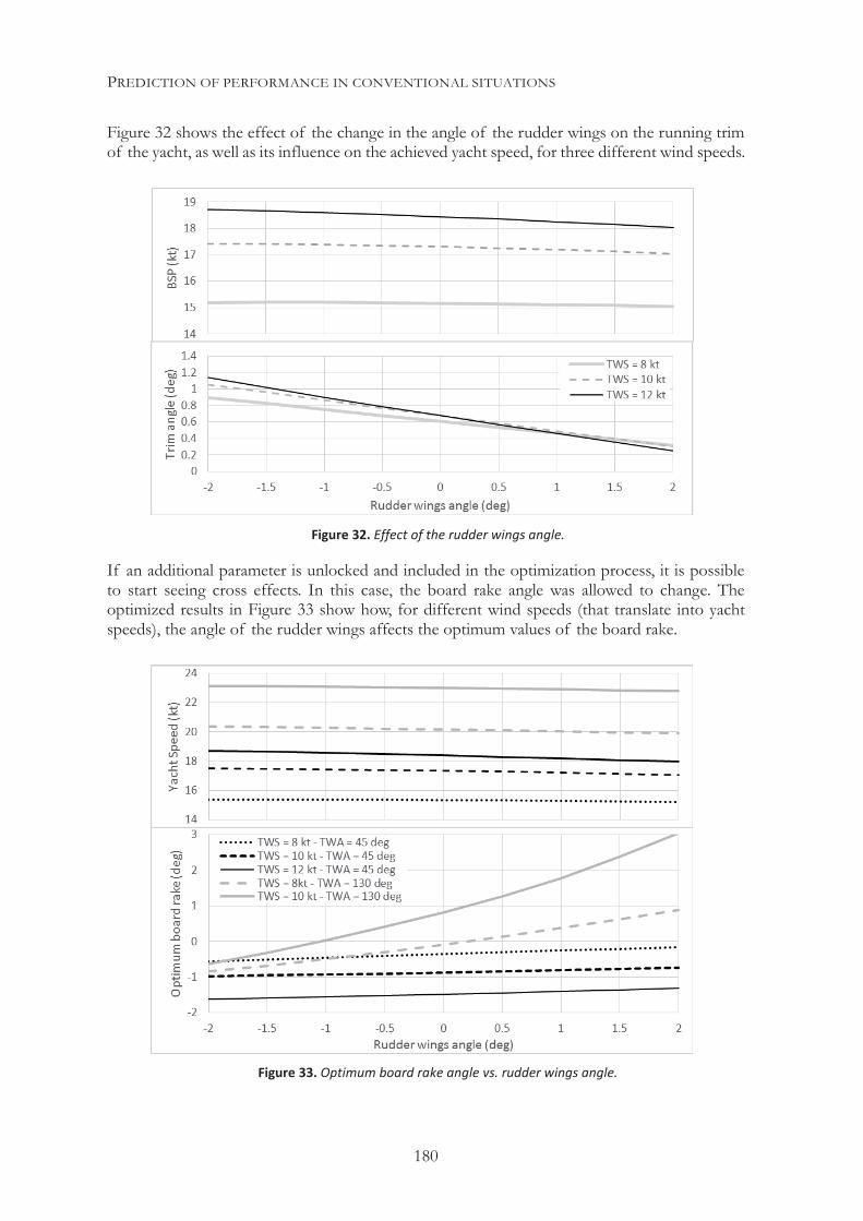
PREDICTION OF PERFORMANCE IN CONVENTIONAL SITUATIONS
180
Figure 32 shows the effect of the change in the angle of the rudder wings on the running trim of the yacht, as well as its influence on the achieved yacht speed, for three different wind speeds.
If an additional parameter is unlocked and included in the optimization process, it is possible to start seeing cross effects. In this case, the board rake angle was allowed to change. The optimized results in Figure 33 show how, for different wind speeds (that translate into yacht speeds), the angle of the rudder wings affects the optimum values of the board rake.
Figure 32. Effect of the rudder wings angle.
Figure 33. Optimum board rake angle vs. rudder wings angle.
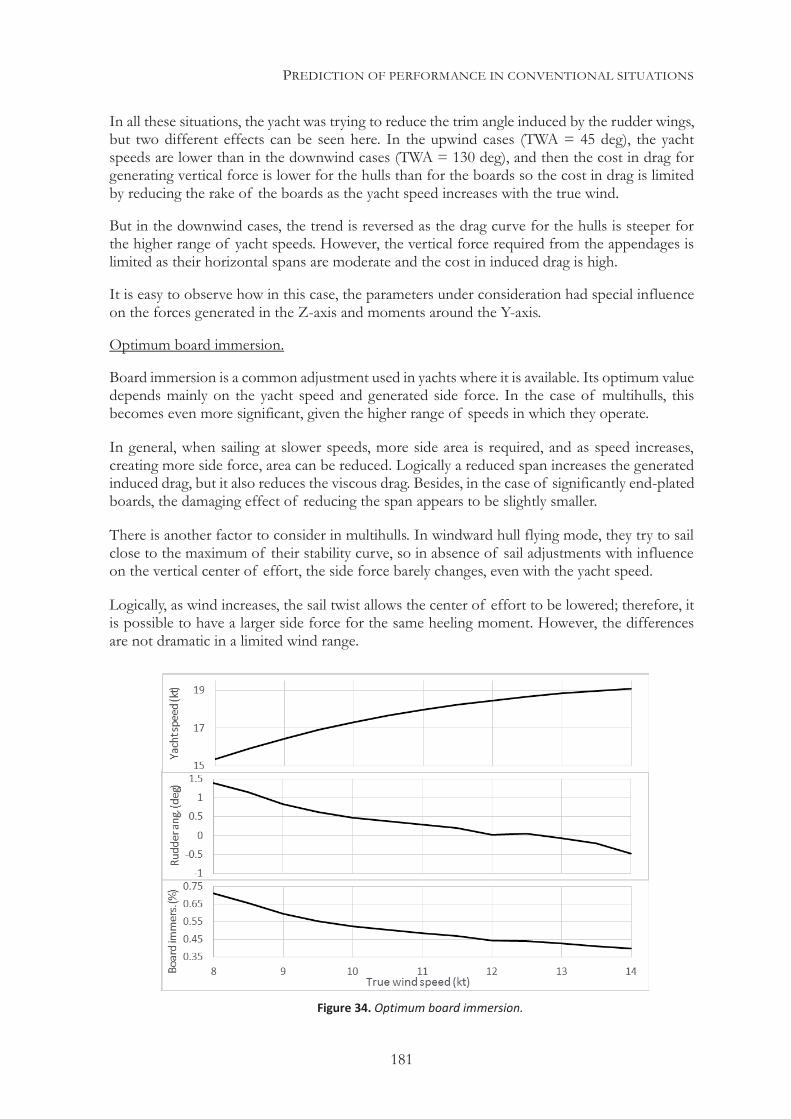
PREDICTION OF PERFORMANCE IN CONVENTIONAL SITUATIONS
181
In all these situations, the yacht was trying to reduce the trim angle induced by the rudder wings, but two different effects can be seen here. In the upwind cases (TWA = 45 deg), the yacht speeds are lower than in the downwind cases (TWA = 130 deg), and then the cost in drag for generating vertical force is lower for the hulls than for the boards so the cost in drag is limited by reducing the rake of the boards as the yacht speed increases with the true wind.
But in the downwind cases, the trend is reversed as the drag curve for the hulls is steeper for the higher range of yacht speeds. However, the vertical force required from the appendages is limited as their horizontal spans are moderate and the cost in induced drag is high.
It is easy to observe how in this case, the parameters under consideration had special influence on the forces generated in the Z-axis and moments around the Y-axis.
Optimum board immersion.
Board immersion is a common adjustment used in yachts where it is available. Its optimum value depends mainly on the yacht speed and generated side force. In the case of multihulls, this becomes even more significant, given the higher range of speeds in which they operate.
In general, when sailing at slower speeds, more side area is required, and as speed increases, creating more side force, area can be reduced. Logically a reduced span increases the generated induced drag, but it also reduces the viscous drag. Besides, in the case of significantly end-plated boards, the damaging effect of reducing the span appears to be slightly smaller.
There is another factor to consider in multihulls. In windward hull flying mode, they try to sail close to the maximum of their stability curve, so in absence of sail adjustments with influence on the vertical center of effort, the side force barely changes, even with the yacht speed.
Logically, as wind increases, the sail twist allows the center of effort to be lowered; therefore, it is possible to have a larger side force for the same heeling moment. However, the differences are not dramatic in a limited wind range.
Figure 34. Optimum board immersion.
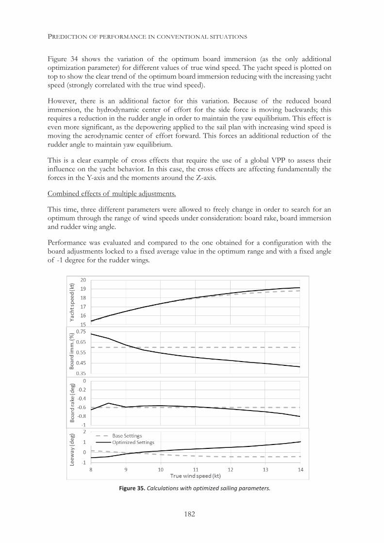
PREDICTION OF PERFORMANCE IN CONVENTIONAL SITUATIONS
182
Figure 34 shows the variation of the optimum board immersion (as the only additional optimization parameter) for different values of true wind speed. The yacht speed is plotted on top to show the clear trend of the optimum board immersion reducing with the increasing yacht speed (strongly correlated with the true wind speed).
However, there is an additional factor for this variation. Because of the reduced board immersion, the hydrodynamic center of effort for the side force is moving backwards; this requires a reduction in the rudder angle in order to maintain the yaw equilibrium. This effect is even more significant, as the depowering applied to the sail plan with increasing wind speed is moving the aerodynamic center of effort forward. This forces an additional reduction of the rudder angle to maintain yaw equilibrium.
This is a clear example of cross effects that require the use of a global VPP to assess their influence on the yacht behavior. In this case, the cross effects are affecting fundamentally the forces in the Y-axis and the moments around the Z-axis.
Combined effects of multiple adjustments.
This time, three different parameters were allowed to freely change in order to search for an optimum through the range of wind speeds under consideration: board rake, board immersion and rudder wing angle.
Performance was evaluated and compared to the one obtained for a configuration with the board adjustments locked to a fixed average value in the optimum range and with a fixed angle of -1 degree for the rudder wings.
Figure 35. Calculations with optimized sailing parameters.
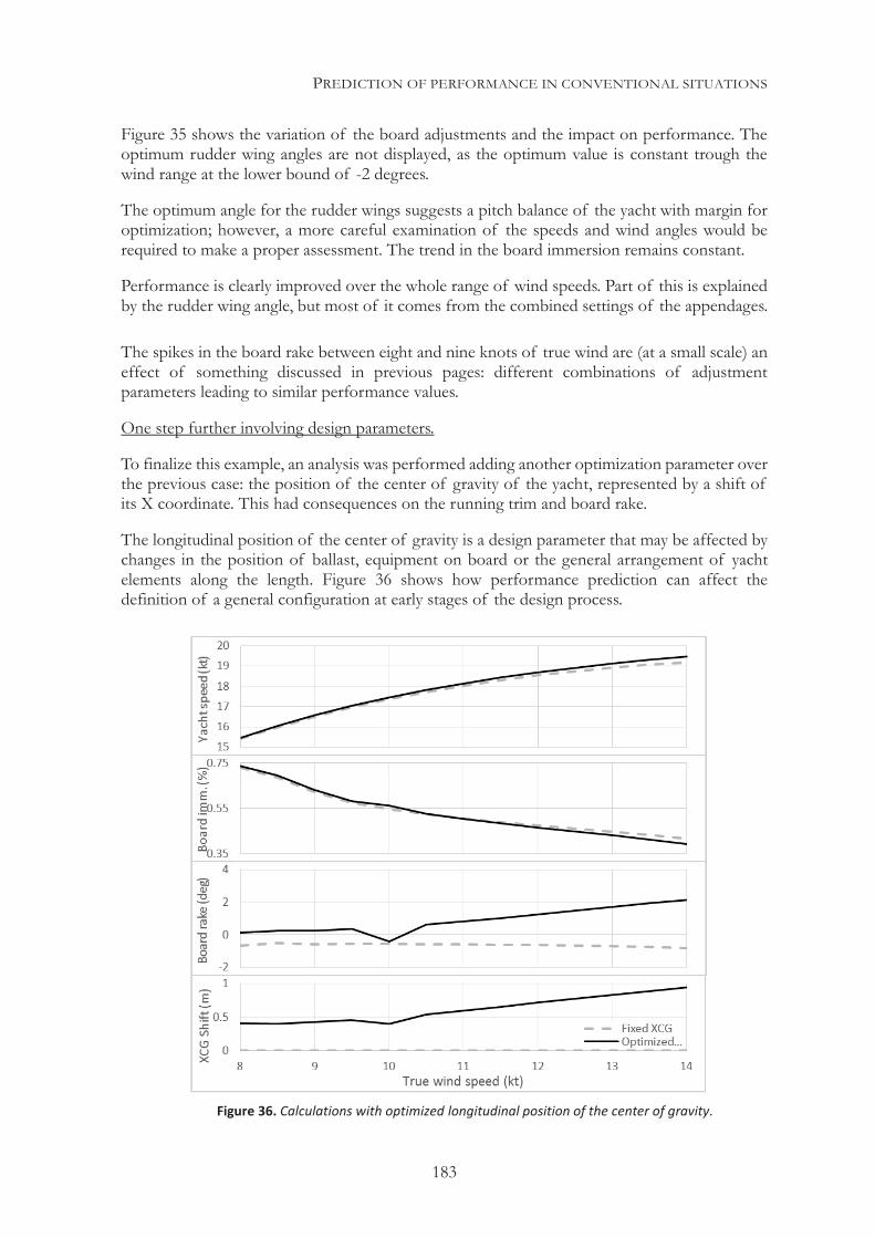
PREDICTION OF PERFORMANCE IN CONVENTIONAL SITUATIONS
183
Figure 35 shows the variation of the board adjustments and the impact on performance. The optimum rudder wing angles are not displayed, as the optimum value is constant trough the wind range at the lower bound of -2 degrees.
The optimum angle for the rudder wings suggests a pitch balance of the yacht with margin for optimization; however, a more careful examination of the speeds and wind angles would be required to make a proper assessment. The trend in the board immersion remains constant.
Performance is clearly improved over the whole range of wind speeds. Part of this is explained by the rudder wing angle, but most of it comes from the combined settings of the appendages.
The spikes in the board rake between eight and nine knots of true wind are (at a small scale) an effect of something discussed in previous pages: different combinations of adjustment parameters leading to similar performance values.
One step further involving design parameters.
To finalize this example, an analysis was performed adding another optimization parameter over the previous case: the position of the center of gravity of the yacht, represented by a shift of its X coordinate. This had consequences on the running trim and board rake.
The longitudinal position of the center of gravity is a design parameter that may be affected by changes in the position of ballast, equipment on board or the general arrangement of yacht elements along the length. Figure 36 shows how performance prediction can affect the definition of a general configuration at early stages of the design process.
Figure 36. Calculations with optimized longitudinal position of the center of gravity.
PREDICTION OF PERFORMANCE IN CONVENTIONAL SITUATIONS
184
For 10 knots of true wind speed, the board rake has been locked to an arbitrary value in order to create a spike in one of the optimization parameters. Spikes are not uncommon and happen “naturally” especially when the number of parameters involved in the optimization that have cross influences increases.
In this case, it can be seen that because of the spike created in the board rake, both the board immersion and optimum longitudinal position of the center of gravity (XCG) are affected and forced out of the trend relative to the true wind speed. However, the change in performance with this new combination of optimum parameters is, once again, negligible.
This suggests, as it has been stated before, the convenience to lock some adjustment parameters when trying to analyze the effect of one specific parameter on performance, before learning about the consequences of cross interactions. Otherwise, there is an added factor of uncertainty, due to the potentially uneven distribution of errors through the parametric space that a model covers, that could mask an actual improvement.
If there is a qualitative change in the solution as all parameters but one are kept constant, and that change provides an improvement in performance, then it is possible to extend that improvement to other combinations of parameters.
Looking at the physical aspects of these results, they suggest that the center of gravity of the yacht is placed too far aft, especially if the yacht is going to sail upwind in good breeze. The increase in performance would clearly support a design decision to act on this, only to be balanced with the increased risk of pitch poling.
It is interesting to observe how the board rake increases more with the yacht speed than it did with the original fixed center of gravity, in order to prevent the trim angle from being excessively bow down.
PREDICTION OF PERFORMANCE IN NON-CONVENTIONAL SITUATIONS
185
9| PERFORMANCE PREDICTION IN NON-CONVENTIONAL SITUATIONS
Besides the situations considered conventional in Chapter 8, there are uses for performance prediction tools which are less obvious but permit to extend their application to other types of analyses.
These other types of analyses include, for instance, the realization of studies with a broader scope than a deterministic performance prediction, by combining different tools. Another use to be highlighted is the analysis of the yacht behavior in the time domain.
The next sections will show different examples of the utilization of performance prediction tools for some of these tasks.
MONOHULL TIME-DOMAIN ACCELERATION CALCULATION The simplest possible case for a time-domain analysis happens when a yacht is sailing at a slower speed than the optimum for a given set of conditions.
This may be due to different reasons, from a change in wind conditions due to a gust or wind shift, to a down-speed situation (a situation in which the yacht is going slower than its potential speed for the corresponding wind conditions) coming out of a tack. In this situation, the objective is to help the yacht to progress as fast as possible to the optimum condition, in order to minimize the losses in the process.
This can become a complex task, involving not only changes in the adjustment parameters but also in the steered course. It may also include taking advantage of induced apparent wind changes to maximize acceleration or, for instance, to respond in the most efficient way to a significant wind shift.
With this type of analysis, we can enter the field of routing calculation, opening a full new landscape for dynamic handling optimization. Rather than limiting the routes to geographic variables, a complete analysis would extend them to the parametric space of all the adjustment variables, with the addition of time.
However, in this example we have intentionally limited the analysis to a basic situation, in order to describe the process involving a very simple autopilot to assist in the progression of the yacht.
9.1.1 THE ANALYSIS SETUP
For this analysis, one of the AC90 yachts already used in the example described in section 8.1 was exposed to a down-speed situation after a tack, and then was left to accelerate until it reached the optimum steady state for the existing wind conditions.
Throughout the transition, the course and rudder angle were locked at a fixed value, and only the sail plan adjustment parameters were allowed to change over time.
PREDICTION OF PERFORMANCE IN NON-CONVENTIONAL SITUATIONS
186
The aerodynamic model used was one already mentioned in that example, built from a matrix of points run in the SK2V code. This model has three possible adjustments: traveler position, twist and flat. For the calculation of the hydrodynamic forces, the model based on the numerical results was chosen from the two models available in that example.
The yacht roll motions were taken into account to consider the induced aerodynamic and hydrodynamic flows, providing a significant damping. Masses and moments of inertia were considered and estimated from a standard list of weights for the yacht. No added masses were taken into account given the type of motions to which the yacht would be exposed (some roll motion and slow linear accelerations).
A Runge-Kutta fourth order method was used for solving the differential equations, calculating the yacht motions over time, with heave, pitch and yaw motions constrained to have no accelerations. The time step used was 0.1 seconds.
9.1.2 THE DIFFERENT CALCULATIONS
These calculations were performed in an upwind sailing situation, in which the parameter to optimize would normally be the component of the yacht speed in the wind axis (VMG), but since the course was locked, with the true wind angle being constant the yacht speed provided the same answer.
The main difficulty during this analysis was defining the criteria to be used by the sail trim autopilots to make the adjustments. Ideally, the optimum progression of the yacht would not only minimize the acceleration time, but also maximize the distance sailed between the start of the acceleration and the point where the steady-state optimum had been reached.
The yacht was intentionally deprived from one of the main resources available to increase speed, that is the ability to bear away in order to accelerate faster, at the expense of some distance lost to windward.
Three different criteria were used for the sail trim. The corresponding acceleration curves were calculated with each one of them.
In the first criterion, the sail parameters were set for the optimum steady-state condition and those values were left constant during the whole process.
In the second and third criteria, for every time step, an optimization process took place in order to calculate the sail adjustments that would maximize the driving force for the apparent wind to which the yacht was exposed at each moment in time. A limit was set for the maximum heeling force that could be produced, using the value corresponding to the calculated steady-state optimum for the wind conditions.
The second criterion was only allowed to adjust the flat parameter, while the third one could also adjust the twist. The traveler position was fixed. The fixed parameters had a constant value corresponding to the steady-state optimum.
No restrictions were applied to the heel angle, since there was plenty of stability available and the yacht was still sailing near the maximum positive slope of the stability curve. The rate of change of the sail trim parameters was left free so oscillations induced by adjustments could be observed.
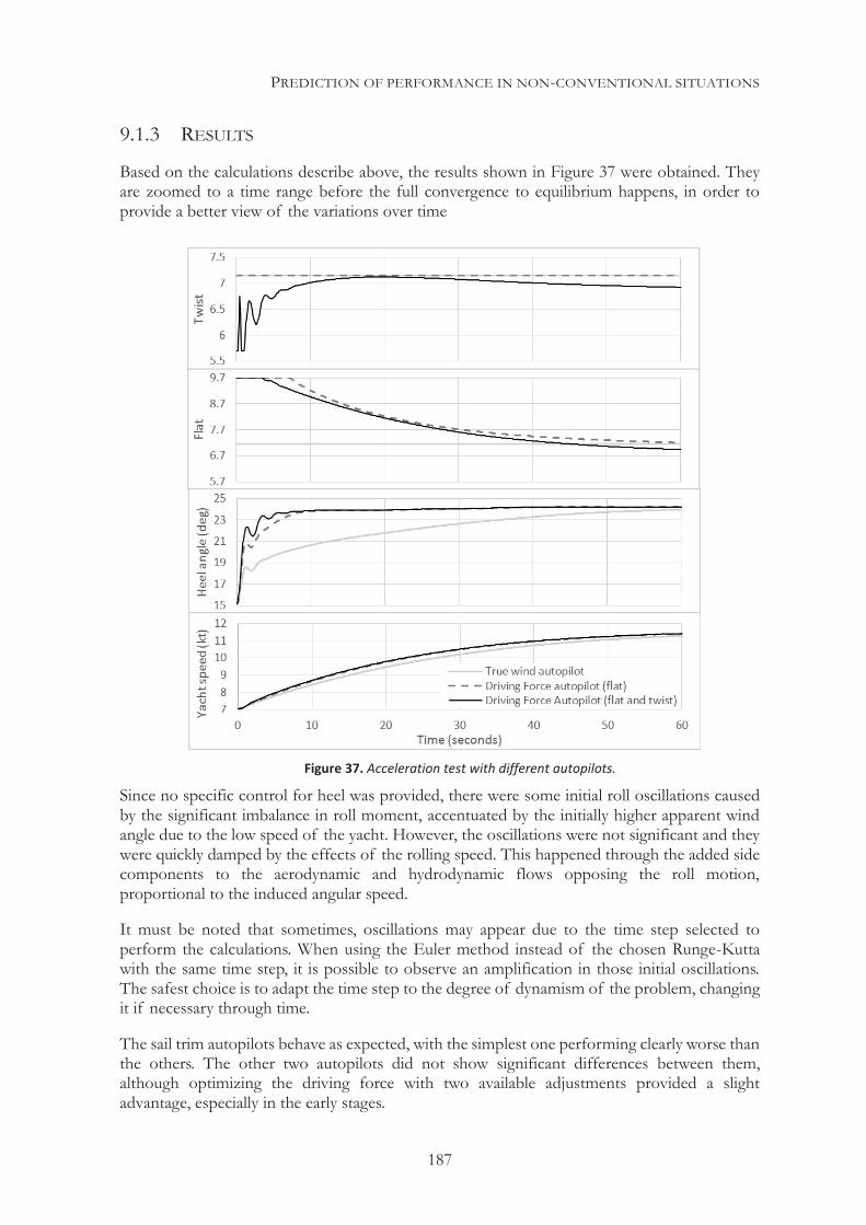
PREDICTION OF PERFORMANCE IN NON-CONVENTIONAL SITUATIONS
187
9.1.3 RESULTS
Based on the calculations describe above, the results shown in Figure 37 were obtained. They are zoomed to a time range before the full convergence to equilibrium happens, in order to provide a better view of the variations over time
Since no specific control for heel was provided, there were some initial roll oscillations caused by the significant imbalance in roll moment, accentuated by the initially higher apparent wind angle due to the low speed of the yacht. However, the oscillations were not significant and they were quickly damped by the effects of the rolling speed. This happened through the added side components to the aerodynamic and hydrodynamic flows opposing the roll motion, proportional to the induced angular speed.
It must be noted that sometimes, oscillations may appear due to the time step selected to perform the calculations. When using the Euler method instead of the chosen Runge-Kutta with the same time step, it is possible to observe an amplification in those initial oscillations. The safest choice is to adapt the time step to the degree of dynamism of the problem, changing it if necessary through time.
The sail trim autopilots behave as expected, with the simplest one performing clearly worse than the others. The other two autopilots did not show significant differences between them, although optimizing the driving force with two available adjustments provided a slight advantage, especially in the early stages.
Figure 37. Acceleration test with different autopilots.
PREDICTION OF PERFORMANCE IN NON-CONVENTIONAL SITUATIONS
188
Since no limitation in the rate of change of the adjustments was used, it is possible to observe for the third autopilot, how the two available sail adjustments (flat and twist) oscillate in a coupled way during the search for optimum settings, but with only a small influence on the actual driving force. This is characteristic of sail models based on experiments where some cross effects between parameters are not properly accounted for, or when extrapolating outside of their range of validity. In the present case, in the beginning of the acceleration, the apparent wind angles were at times outside of the valid range of variation for the model, due to the side component induced by the roll motion.
It must be noted that the same analysis could have been performed using variable wind conditions continuously changing over time, instead of constant ones. This does not add any complexity to the calculations, and the adjustment criteria used by the autopilots would be adjusting the sails to adapt to the instant wind conditions in the same exact way. The next example will expand on this type of analysis, putting it in practice with a very different purpose.
ANALYSIS OF COLLECTED FULL-SCALE SAILING DATA Full-scale testing is a tremendously challenging task. Given that sailing takes place in an always-changing environment, the test conditions are always far from ideal laboratory conditions. This makes full-scale performance evaluation difficult, even if it would be possible to record those changing conditions with perfect accuracy. For that reason, the most common setup when testing on the water is to do it with two similar yachts.
The yachts are positioned sailing as close as possible to each other without having any mutual interference (mostly in their apparent winds), and then, performance is compared over several minutes of reasonably stable conditions. The test is often repeated several times, also including changes in the yachts relative positions. This is done to remove local conditions (like a gradually changing wind angle with time or geographic position), and even subjective elements.
However, even with all those cautions, the changes in the wind speed and direction for each yacht make the evaluation of the results extremely difficult. They also force to make a significant number of repeats, so that statistics help filter out the noise generated by those changes.
9.2.1 THE ENVIRONMENTAL CROSSROAD
Wind changes are the main factor responsible for these difficulties, and more precisely the different changes each yacht is exposed to, but the way the sailors react to those changes also affects the measured performance. For this reason, the yachts have information about each other’s adjustments and sailing conditions. This way, when a wind change affects similarly both yachts, it is possible to mimic the reactions so the added noise of a different adjustment is minimized.
The problem is that despite having the yachts sailing in close proximity, they are still exposed to different wind variations. A same change may reach each yacht at a different time, or a narrow gust for instance may affect only one of the yachts.
This makes the task of extracting valid conclusions from a long session of testing on the water even harder. And that is assuming that the data recorded in each yacht (especially the wind information) is perfectly accurate. The wind measurement is another difficult task and an additional source of errors, with some consequences that will be briefly discussed at the end of this example.
PREDICTION OF PERFORMANCE IN NON-CONVENTIONAL SITUATIONS
189
9.2.2 A PROPOSED SOLUTION TO REDUCE UNCERTAINTY
The solution proposed here is very simple. It consists in using two identical virtual yachts that will “be sailed” in the same wind conditions as measured for each real counterpart in an on-the-water test.
These two yachts will see their relative performance change with the varying wind conditions through the duration of the test. However, this change in performance will depend solely on the environmental conditions under which they are sailing, as the virtual yachts are identical (and thus, the mathematical models that characterize them).
If the differences between the virtual yachts are deducted from the differences between the recorded data corresponding to the actual yachts, we will (ideally) be filtering out the differences in performance due to the different wind conditions in which the yachts are sailing. That way, the corrected differences will depend exclusively on the performance differences between the yachts, even if they are still affected by the different adjustments made by the sailors on board. However, if sufficiently complex models are available, especially models for aerodynamic forces, it is possible to also consider some of the actual on-board adjustments and reproduce them in the virtual yachts.
But the truth is that even the simplest virtual yacht with default adjustments can help significantly to reduce the level of uncertainty from the tests.
This process would normally be applied as post-processing on recorded data, but it is also possible to have the virtual yacht running in real time with the data measured as the yacht is sailing . This provides a powerful real time filter that can be used to improve the usefulness for a test session.
9.2.3 THE CALCULATIONS
For the calculations of the example, AC Class yachts (used in the America’s Cup between 1992 and 2007) were chosen. A generic configuration of hull and appendages was created and run through the panel code Splash.
All the mathematical models used for the calculation of forces were similar to those described in the example of section 8.1, with the only difference of the type of yacht.
The recorded sailing data used corresponds to a sample of 400 seconds belonging to a specific test performed during an on-the-water test session with two similar yachts.
The yachts were run through the recorded data in a time-domain analysis using a Runge-Kutta fourth order method, in a similar situation to the one described in the example of section 9.1, with the depowering parameters adjusted to reproduce the optimum settings for the true wind conditions in which the yachts were sailing.
The virtual yachts were also forced to sail the same course over ground (COG) as their real counterparts. Given that the test was made to optimize upwind performance, the progress against the wind, based on the yacht speeds combined with the sailed courses and the measured wind directions, would provide a measurement of their relative performance. Comparing the differences in the progress of one yacht relative to the other, it is possible to define a relative gain and a gain rate as a simple and robust objective function.
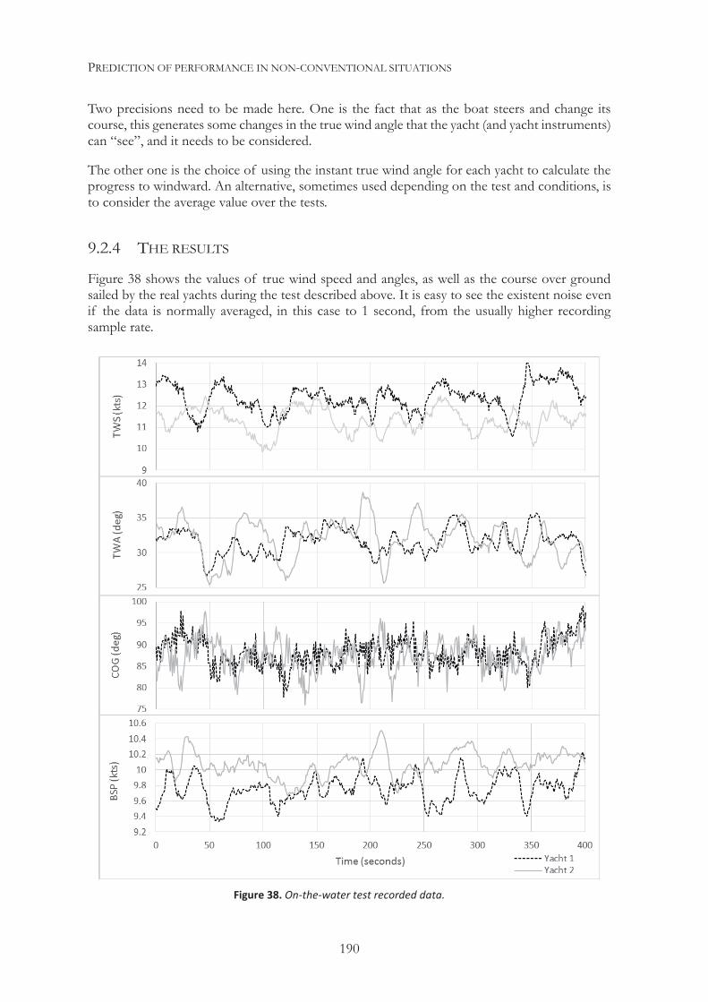
PREDICTION OF PERFORMANCE IN NON-CONVENTIONAL SITUATIONS
190
Two precisions need to be made here. One is the fact that as the boat steers and change its course, this generates some changes in the true wind angle that the yacht (and yacht instruments) can “see”, and it needs to be considered.
The other one is the choice of using the instant true wind angle for each yacht to calculate the progress to windward. An alternative, sometimes used depending on the test and conditions, is to consider the average value over the tests.
9.2.4 THE RESULTS
Figure 38 shows the values of true wind speed and angles, as well as the course over ground sailed by the real yachts during the test described above. It is easy to see the existent noise even if the data is normally averaged, in this case to 1 second, from the usually higher recording sample rate.
Figure 38. On-the-water test recorded data.
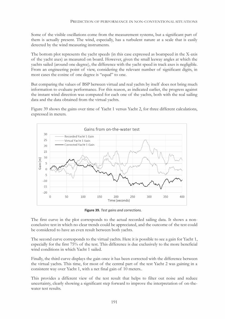
PREDICTION OF PERFORMANCE IN NON-CONVENTIONAL SITUATIONS
191
Some of the visible oscillations come from the measurement systems, but a significant part of them is actually present. The wind, especially, has a turbulent nature at a scale that is easily detected by the wind measuring instruments.
The bottom plot represents the yacht speeds (in this case expressed as boatspeed in the X-axis of the yacht axes) as measured on board. However, given the small leeway angles at which the yachts sailed (around one degree), the difference with the yacht speed in track axes is negligible. From an engineering point of view, considering the relevant number of significant digits, in most cases the cosine of one degree is “equal” to one.
But comparing the values of BSP between virtual and real yachts by itself does not bring much information to evaluate performance. For this reason, as indicated earlier, the progress against the instant wind direction was computed for each one of the yachts, both with the real sailing data and the data obtained from the virtual yachts.
Figure 39 shows the gains over time of Yacht 1 versus Yacht 2, for three different calculations, expressed in meters.
The first curve in the plot corresponds to the actual recorded sailing data. It shows a non-conclusive test in which no clear trends could be appreciated, and the outcome of the test could be considered to have an even result between both yachts.
The second curve corresponds to the virtual yachts. Here it is possible to see a gain for Yacht 1, especially for the first 75% of the test. This difference is due exclusively to the more beneficial wind conditions in which Yacht 1 sailed.
Finally, the third curve displays the gain once it has been corrected with the difference between the virtual yachts. This time, for most of the central part of the test Yacht 2 was gaining in a consistent way over Yacht 1, with a net final gain of 10 meters..
This provides a different view of the test result that helps to filter out noise and reduce uncertainty, clearly showing a significant step forward to improve the interpretation of on-the-water test results.
Figure 39. Test gains and corrections.
PREDICTION OF PERFORMANCE IN NON-CONVENTIONAL SITUATIONS
192
However, this process is not exempt of problems and risks. The next lines will discuss the most significant problem, along with suggestions to minimize its negative impact.
9.2.5 A NOTE ON INSTRUMENTS CALIBRATION AND CURRENT
Instruments calibration
Given that the strategy of the proposed method relies on the recorded wind data, it is important to make every effort to produce accurate calibrations of the wind instruments in both yachts, and to install the instruments on board in a way that permits to maintain this accuracy. This includes having the instruments placed in the same position in both yachts (in height and relative proximity to the sails), and verifying their alignment.
Sailing a virtual yacht through wind data that has a systematic bias will lead to systematically biased performance predictions. The differences in the calibrations or alignments will be perceived as differences in wind, and this will seriously mislead the interpretation of the results.
This issue cannot be stressed enough, given how difficult it is to guarantee that the wind is being read the same way from two different sets of instruments installed on top of a mast that bends, twists and is constantly under the influence of motions. It must be noted that wind readings are corrected for the motions to which the wind instruments are exposed, as well as for yacht speed. For this reason, inaccuracy in the instruments reading the boat attitude, motions and speed will also lead to errors in the deduced true wind.
It is possible to perform “post sailing” calibrations, comparing readings on different tacks over multiple tests and searching for systematic biases in the speed and angle of the wind readings. This is a complicated process, but it can provide the required information to correct a situation that would otherwise make the data useless (or dangerously misleading if the problem is not even identified)
Current
Current is another factor that can easily distort the results of full-scale tests, also affecting the correct performance of the virtual yachts. Current adds a component to the wind triangle for the calculation of the true wind from the measured apparent wind. If an existent current is ignored, the deduced true wind in which the yachts have sailed (and which has been used to run the virtual yachts) will be wrong both in speed and angle.
For this reason, when possible, current should be measured and taken into account. To help with this problem, the use of accurate GPS on board permits to calculate speeds and courses over ground, which can be compared to the on-board measured boatspeed and course (assuming some knowledge about the leeway, that will also appear in that comparison, mixed with the current effect). Doing some sailing on opposite tacks before starting actual tests (and processing that data to evaluate the presence of current) can actually provide a reasonably good indication of the current at that moment, so that it can be used to correct the wind data.
An estimate of the current during the test can also be calculated afterwards, based on the recorded data, following the previous procedure.
These kinds of “post-sailing” calibrations and corrections are complex, but the development of procedures to better identify distorting factors during full-scale tests is an area of
PREDICTION OF PERFORMANCE IN NON-CONVENTIONAL SITUATIONS
193
considerable interest. They can significantly increase the level of trust in the sailing data and improve its role in assessing performance.
STUDY OF FEASIBLE SAILING POINTS As it was seen in the example of section 8.2, there may be more than one optimum solution to a steady-state calculation. Even ignoring the usually present “very slow” cases, which are easy to identify and discard, sometimes there remains more than one “fast” solution. The number of potential local optima also increases with the number of optimization variables, depending on their physical effects and degree of coupling.
But the example we are referring to described a common sailing situation with a reduced set of adjustments and optimization parameters available. It was the change in the apparent wind speed that made a qualitative difference, permitting to achieve a situation in which the driving force was increased by the order of 50% with no change in course. This is a common situation in multihulls, where the possible range of variation for yacht speeds is significant, even for a narrow range of wind speeds.
However, some of these solutions may not be achievable, since the drag will increase with the wind and yacht speeds before the drag curve provides some “relief ” in terms of reducing its slope with the yacht speed. That would imply that there may not be a valid transition path between the slower calculated solution and a theoretically faster one.
A good analogy to this situation happens with surfers in waves with a long period. These waves have a lower slope, so the component of the gravity force helping the surfer is often insufficient to overcome the surfboard drag before it is in a full planing situation (where drag decreases). The solution comes from towing the surfer in the slope of the wave, until he reaches a full planing regime, and then he is left on his own, able to maintain a surfing situation.
The objective of this example is to show one of the possible transition paths between the two different sailing modes seen in section 8.2. It is important to keep in mind that, sometimes, that path may not even exist (as it happened with the “cheating” surfer analogy).
9.3.1 THE CALCULATIONS
Going back to the example we are referring to, we selected the sailing situation with a true wind angle of 130 degrees and a true wind speed of 7 knots. For that situation, there were two possible solutions, shown in Table 8.
With all board and rudder wing adjustments left unchanged, the key difference between the solutions was the effect of the augmented apparent wind speed. By changing some of these appendage adjustments, it may be possible to “force” the high-speed mode, as well as by carefully choosing initial values that provide a high apparent wind speed to start with.
But according to the previous results, if the wind is slowly increasing over a yacht sailing a constant course, until the wind reaches a speed of 7.5 knots, the yacht will not enter into the fast mode unless something else is done.
In this example, the effect of slightly altering the course to sail closer to the wind was evaluated. By doing that, the true wind angle changed with the course change, permitting the apparent
PREDICTION OF PERFORMANCE IN NON-CONVENTIONAL SITUATIONS
194
wind speed to increase enough to “jump” into the fast mode. Then the yacht started to slowly bear away to the same course and true wind angle, this time sailing in the fast mode.
Doing this process, we have defined a time-domain transition path that may not always be present, but that in this case provides a way to reach that fast mode.
But given that the yacht is sailing around the maximum of the stability curve, some actions may be required to adjust the sail plan power to prevent capsizing. This would be achieved by using a specific autopilot.
This autopilot consists of a PID controller that adjusts the flat parameter of the sail plan to maintain the heel angle when flying the windward hull. This controller has proved capable to maintain a target heel angle in those conditions with minimal oscillations. In this case, the target is, as before, the heel angle that allows the windward hull to fly 0.5 meters above the water, taking into account the existing sinkage.
An additional pilot was responsible to slowly steer the yacht to a higher course until the windward hull would “take off ” and then it started to slowly go back to the original course. In this case, the pilot changed the rudder angle following a predefined curve, result of a trial and error study.
The situation begins with the yacht sailing in a stationary state in the low-speed mode that is maintained for two seconds. Then it starts to steer into the wind. All the maneuvers were performed intentionally slow to avoid significant dynamic effects.
9.3.2 THE RESULTS
Figure 40 shows the first 100 seconds of the 180 seconds simulation corresponding to this experiment (prior to a slow convergence to the values of the steady-state fast sailing mode). The plots permit to draw an immediate first conclusion: there is a feasible path to the fast sailing mode. Therefore, sailors can actually perform that transition from the slow sailing mode to the fast one (without the use of numerical constraints or “adequate initial values”).
Beyond that first conclusion, a number of observations can be made by examining the plotted values for some of the parameters of the yacht during the maneuver:
Steering was intentionally slow, but it is possible to observe some derived effects. A first effect happens when the rudder starts to reduce its angle, experimenting consequently an immediate reduction in the side force that it generates. This has a direct effect on the leeway, which starts increasing during the turn. This reduction in the hydrodynamic side force also produces an immediate small loss of heeling moment, creating a small but perceptible reduction of the heel angle, visible at the very beginning of the turn.
Although it is not shown in the plots as separated from other effects, as the yacht turns into the wind, there is a small dynamic component increasing the heel moment due to the created centripetal acceleration (which also contributes to increase leeway). The effect is reversed when bearing away back to the original course, inducing a reduction in heel. When faster maneuvers are performed, these dynamic effects can become much more significant and can be used to facilitate the “take off ” of the windward hull.
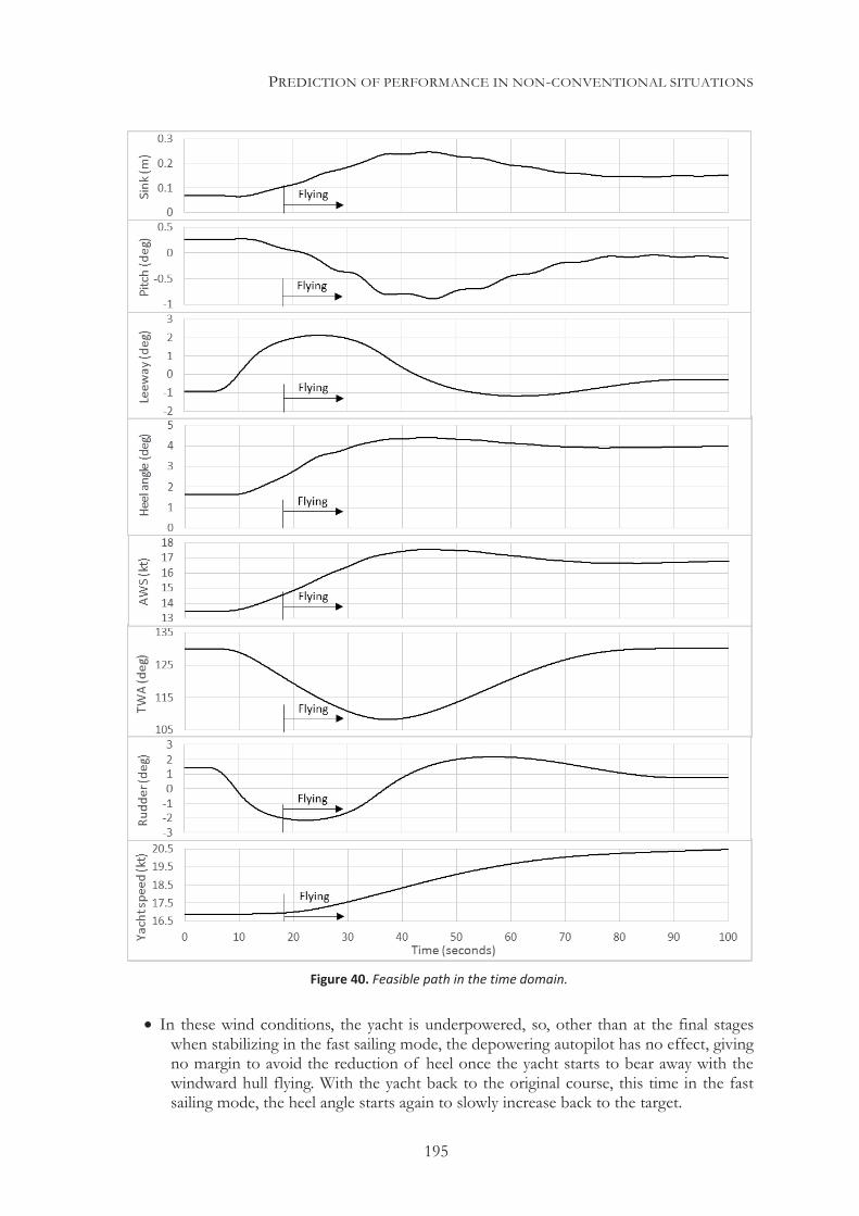
PREDICTION OF PERFORMANCE IN NON-CONVENTIONAL SITUATIONS
195
In these wind conditions, the yacht is underpowered, so, other than at the final stages when stabilizing in the fast sailing mode, the depowering autopilot has no effect, giving no margin to avoid the reduction of heel once the yacht starts to bear away with the windward hull flying. With the yacht back to the original course, this time in the fast sailing mode, the heel angle starts again to slowly increase back to the target.
Figure 40. Feasible path in the time domain.
PREDICTION OF PERFORMANCE IN NON-CONVENTIONAL SITUATIONS
196
The actions of the rudder and increasing apparent wind create some oscillations in pitch, that also translate into oscillations in sinkage and heel, with an oscillation period determined by the weight and moments of inertia of the yacht.
Sinkage changes during this process, increasing with heel angle as more displacement is taken by the leeway hull. However, after the maximum, it starts decreasing again, as the change in the speed of the yacht is also making the board and rudder wings create a larger vertical force. Variations in pitch are also affecting sinkage at the point where it is measured (amidships).
The speed of the yacht is gently increasing through the whole process. The combined effect of the steering (affecting the true wind angle) and of the increase of the yacht speed can be observed in the apparent wind speed.
After the required variations of the rudder angle to steer the yacht, once the yacht is back to the original course the rudder angle is lower for the fast sailing mode than for the original slower sailing mode. This may be surprising, given that only a fraction of the span of the windward rudder is immersed with the windward hull flying, but the higher speed of the incoming flow to the rudder has an even larger influence on the generated side force.
A detailed review of the results reveals other aspects of the process, but one significant lesson learnt is the risk of oscillations.
Once the oscillations of numerical origin are discarded, which are much more present when using the Euler method rather than the Runge-Kutta fourth order method finally selected, the physics involved and the yacht configuration itself make it vulnerable to dynamic instabilities. Some of the reasons are the small waterplane area of the yacht, the incidence of the motions in the vertical forces, the cross effects between degrees of freedom (mainly between sinkage, heel and pitch) and the close, yet different, moments of inertia around the different axes.
The innate human ability for pattern recognition becomes evident when dealing with those oscillations. A trained person can do an excellent job at anticipating, reducing and even eliminating them, using as the main source of perception for those oscillations the accelerations that they generate. This suggests that autopilots based on analyzing angular accelerations can be good candidates in a number of situations. Once again, this is an area where the existent knowledge in control theory can certainly provide significant benefits. Actually, although they require carefully tuning and are not exempt from problems, even simple PID controllers provide a significant improvement over more basic proportional autopilots.
A next step in this type of analysis could be to manually perform in real time the main adjustments, analyzing then the effects on performance and identifying the chances of success in completing the maneuver. However, some intuitive physical user interfaces would be needed to perform the required adjustments.
It is necessary to remind that in order to operate in more dynamic scenarios than the one analyzed here, it is absolutely necessary to have the mathematical models implemented to support the physical phenomena involved. Maneuverability would probably be the first candidate, although some reasonably simple models can already provide most of the required information to handle most of the dynamic problems that we can encounter sailing in flat water.
PREDICTION OF PERFORMANCE IN NON-CONVENTIONAL SITUATIONS
197
INTEGRATION IN A GLOBAL OPTIMIZATION TOOL VPPs are, in most cases, the final users of physical data related to the sailing yacht. This data is processed and used in order to generate a simple picture to describe the yacht’s performance, measured in terms of achievable speeds for different wind conditions.
But some other times, VPPs integrate into projects of a wider scope that, on one hand, can use more sophisticated ways to measure performance, and on the other, can become a more sophisticated optimization process to define what an optimal design can be.
A. Mason’s thesis “Stochastic Optimization of America’s Cup Yachts” (45) provides a perfect example of this, involving a number of different tools and resources to perform a global optimization based on a VPP. This author was responsible for the deterministic part of the performance prediction, developing the VPP component and generating the numerical data used to calculate the hydrodynamic forces in that project.
In the next pages that research will be described, in order to illustrate a not very common use of performance prediction, which involves a number of the problems discussed in previous chapters. The referred thesis, however, provide a complete description of the whole project.
9.4.1 THE OBJECTIVE
The objective of the project was to select the design candidate, in terms of hull shape, that would have the highest probability to win in a series of races (with the structure of the 32nd America’s Cup in 2007) in the weather conditions described by a probability distribution for the race dates.
This type of selection goes well beyond a simple estimate of potential performance in specific wind conditions, for a number of reasons including the following ones:
Performance is not defined in terms of pure speed, but in terms of probability of beating other candidate designs in one-to-one races (match race) through a series of regattas.
In those regattas, the wind will evolve and basic interactions between racing yachts would be taken into account (such as wind blanketing and the freedom to choose a strategy relative to shifting wind).
The wind conditions would respond to a probability distribution based on historical data for the venue and time of the year of interest; therefore, races would be run according to it.
These factors required the use of several components integrated in a managing tool, named VESPA, in order to produce the simulation that will be described briefly in the next section.
9.4.2 DIFFERENT PROBLEMS TO LINK
A number or problems involved in the global process required to face the process from different points of view.
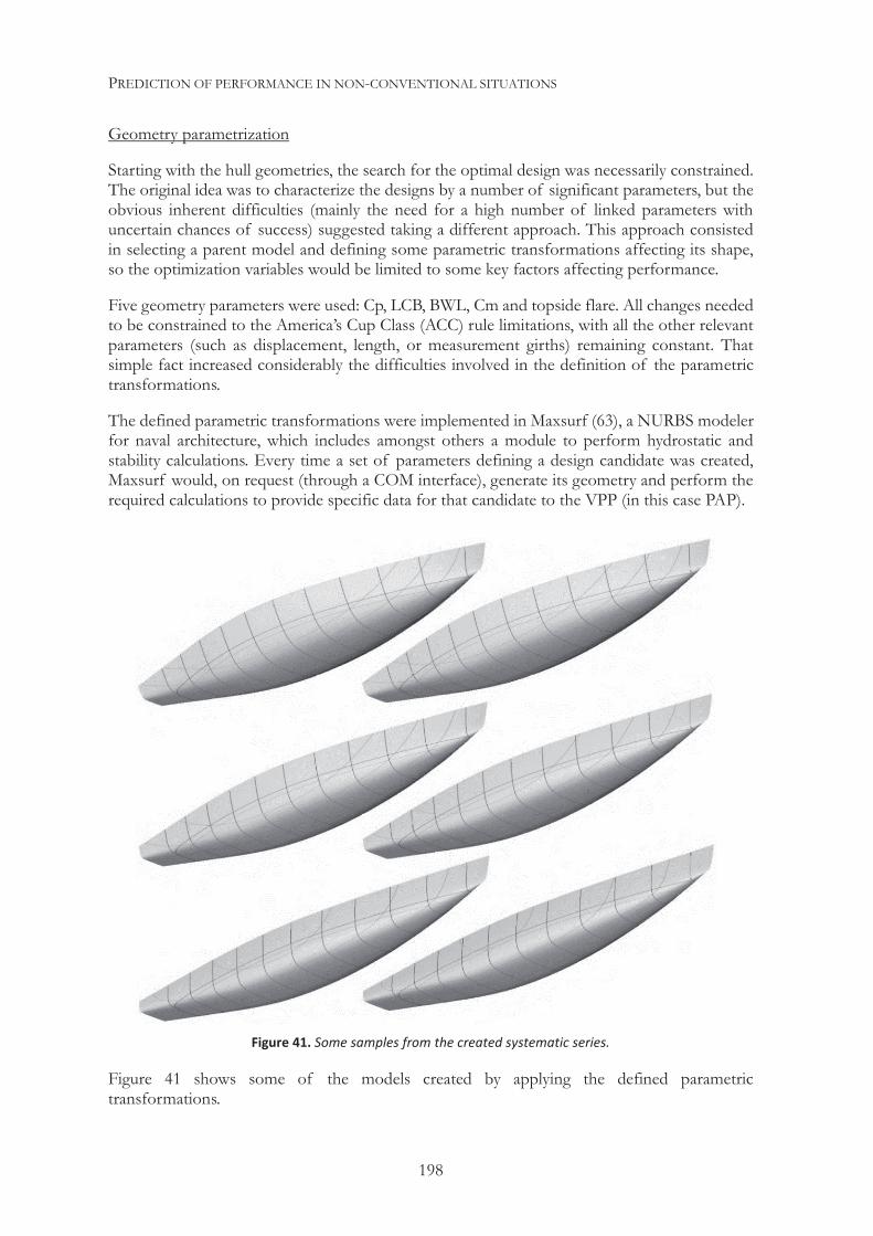
PREDICTION OF PERFORMANCE IN NON-CONVENTIONAL SITUATIONS
198
Geometry parametrization
Starting with the hull geometries, the search for the optimal design was necessarily constrained. The original idea was to characterize the designs by a number of significant parameters, but the obvious inherent difficulties (mainly the need for a high number of linked parameters with uncertain chances of success) suggested taking a different approach. This approach consisted in selecting a parent model and defining some parametric transformations affecting its shape, so the optimization variables would be limited to some key factors affecting performance.
Five geometry parameters were used: Cp, LCB, BWL, Cm and topside flare. All changes needed to be constrained to the America’s Cup Class (ACC) rule limitations, with all the other relevant parameters (such as displacement, length, or measurement girths) remaining constant. That simple fact increased considerably the difficulties involved in the definition of the parametric transformations.
The defined parametric transformations were implemented in Maxsurf (63), a NURBS modeler for naval architecture, which includes amongst others a module to perform hydrostatic and stability calculations. Every time a set of parameters defining a design candidate was created, Maxsurf would, on request (through a COM interface), generate its geometry and perform the required calculations to provide specific data for that candidate to the VPP (in this case PAP).
Figure 41 shows some of the models created by applying the defined parametric transformations.
Figure 41. Some samples from the created systematic series.
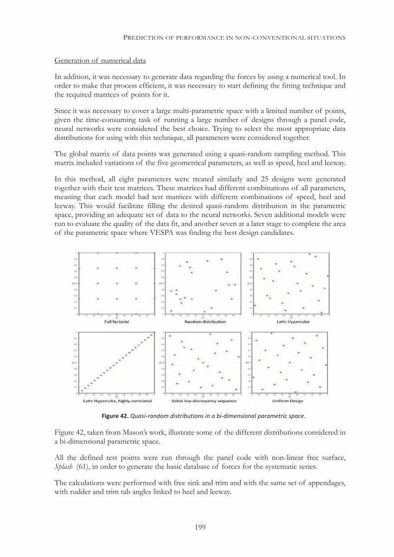
PREDICTION OF PERFORMANCE IN NON-CONVENTIONAL SITUATIONS
199
Generation of numerical data
In addition, it was necessary to generate data regarding the forces by using a numerical tool. In order to make that process efficient, it was necessary to start defining the fitting technique and the required matrices of points for it.
Since it was necessary to cover a large multi-parametric space with a limited number of points, given the time-consuming task of running a large number of designs through a panel code, neural networks were considered the best choice. Trying to select the most appropriate data distributions for using with this technique, all parameters were considered together.
The global matrix of data points was generated using a quasi-random sampling method. This matrix included variations of the five geometrical parameters, as well as speed, heel and leeway.
In this method, all eight parameters were treated similarly and 25 designs were generated together with their test matrices. These matrices had different combinations of all parameters, meaning that each model had test matrices with different combinations of speed, heel and leeway. This would facilitate filling the desired quasi-random distribution in the parametric space, providing an adequate set of data to the neural networks. Seven additional models were run to evaluate the quality of the data fit, and another seven at a later stage to complete the area of the parametric space where VESPA was finding the best design candidates.
Figure 42, taken from Mason’s work, illustrate some of the different distributions considered in a bi-dimensional parametric space.
All the defined test points were run through the panel code with non-linear free surface, Splash (61), in order to generate the basic database of forces for the systematic series.
The calculations were performed with free sink and trim and with the same set of appendages, with rudder and trim tab angles linked to heel and leeway.
Figure 42. Quasi-random distributions in a bi-dimensional parametric space.
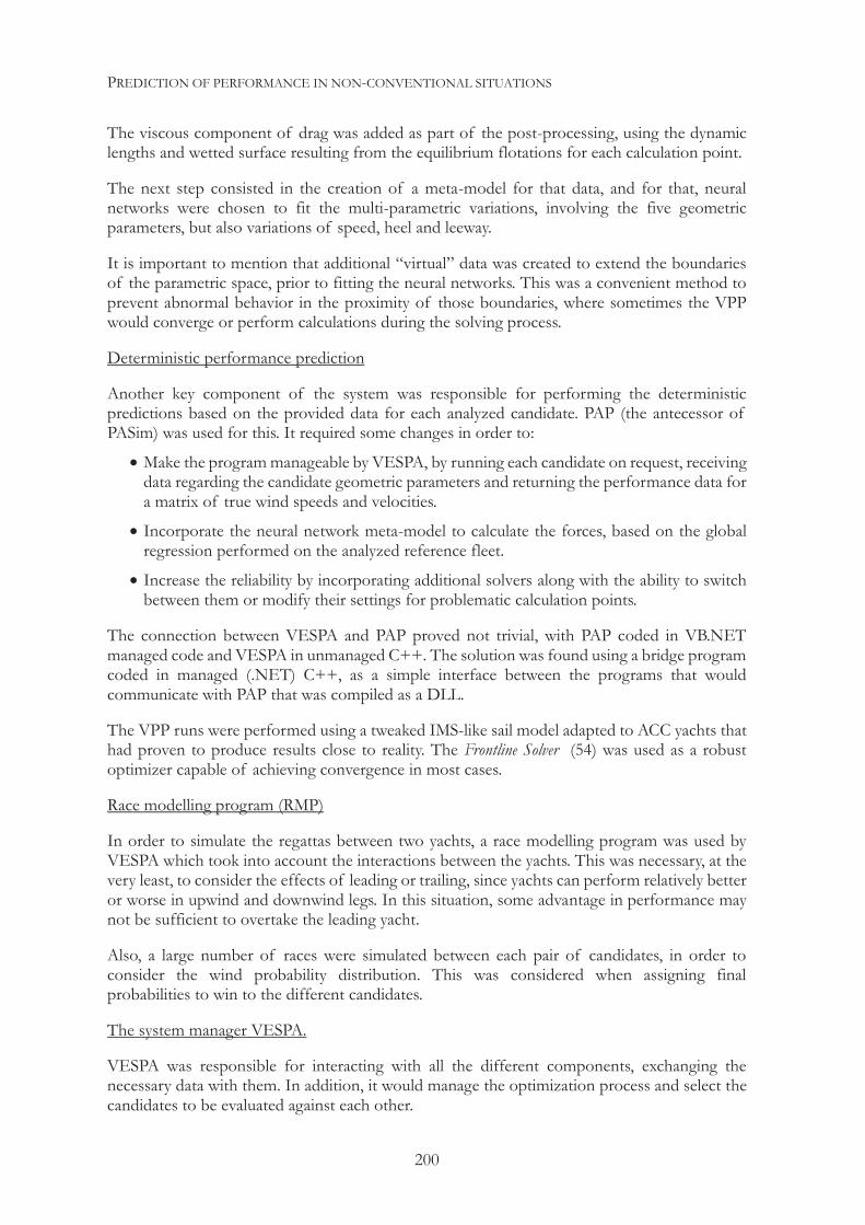
PREDICTION OF PERFORMANCE IN NON-CONVENTIONAL SITUATIONS
200
The viscous component of drag was added as part of the post-processing, using the dynamic lengths and wetted surface resulting from the equilibrium flotations for each calculation point.
The next step consisted in the creation of a meta-model for that data, and for that, neural networks were chosen to fit the multi-parametric variations, involving the five geometric parameters, but also variations of speed, heel and leeway.
It is important to mention that additional “virtual” data was created to extend the boundaries of the parametric space, prior to fitting the neural networks. This was a convenient method to prevent abnormal behavior in the proximity of those boundaries, where sometimes the VPP would converge or perform calculations during the solving process.
Deterministic performance prediction
Another key component of the system was responsible for performing the deterministic predictions based on the provided data for each analyzed candidate. PAP (the antecessor of PASim) was used for this. It required some changes in order to:
Make the program manageable by VESPA, by running each candidate on request, receiving data regarding the candidate geometric parameters and returning the performance data for a matrix of true wind speeds and velocities.
Incorporate the neural network meta-model to calculate the forces, based on the global regression performed on the analyzed reference fleet.
Increase the reliability by incorporating additional solvers along with the ability to switch between them or modify their settings for problematic calculation points.
The connection between VESPA and PAP proved not trivial, with PAP coded in VB.NET managed code and VESPA in unmanaged C++. The solution was found using a bridge program coded in managed (.NET) C++, as a simple interface between the programs that would communicate with PAP that was compiled as a DLL.
The VPP runs were performed using a tweaked IMS-like sail model adapted to ACC yachts that had proven to produce results close to reality. The Frontline Solver (54) was used as a robust optimizer capable of achieving convergence in most cases.
Race modelling program (RMP)
In order to simulate the regattas between two yachts, a race modelling program was used by VESPA which took into account the interactions between the yachts. This was necessary, at the very least, to consider the effects of leading or trailing, since yachts can perform relatively better or worse in upwind and downwind legs. In this situation, some advantage in performance may not be sufficient to overtake the leading yacht.
Also, a large number of races were simulated between each pair of candidates, in order to consider the wind probability distribution. This was considered when assigning final probabilities to win to the different candidates.
The system manager VESPA.
VESPA was responsible for interacting with all the different components, exchanging the necessary data with them. In addition, it would manage the optimization process and select the candidates to be evaluated against each other.
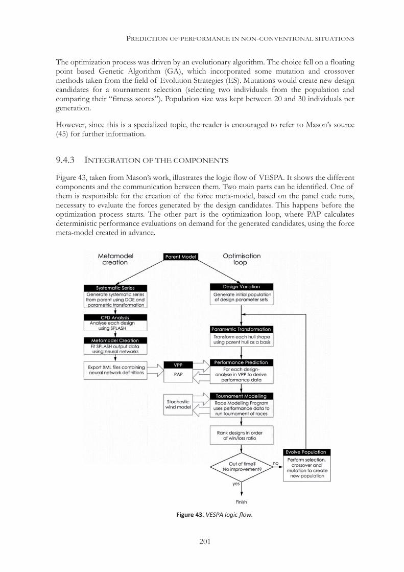
PREDICTION OF PERFORMANCE IN NON-CONVENTIONAL SITUATIONS
201
The optimization process was driven by an evolutionary algorithm. The choice fell on a floating point based Genetic Algorithm (GA), which incorporated some mutation and crossover methods taken from the field of Evolution Strategies (ES). Mutations would create new design candidates for a tournament selection (selecting two individuals from the population and comparing their “fitness scores”). Population size was kept between 20 and 30 individuals per generation.
However, since this is a specialized topic, the reader is encouraged to refer to Mason’s source (45) for further information.
9.4.3 INTEGRATION OF THE COMPONENTS
Figure 43, taken from Mason’s work, illustrates the logic flow of VESPA. It shows the different components and the communication between them. Two main parts can be identified. One of them is responsible for the creation of the force meta-model, based on the panel code runs, necessary to evaluate the forces generated by the design candidates. This happens before the optimization process starts. The other part is the optimization loop, where PAP calculates deterministic performance evaluations on demand for the generated candidates, using the force meta-model created in advance.
Figure 43. VESPA logic flow.
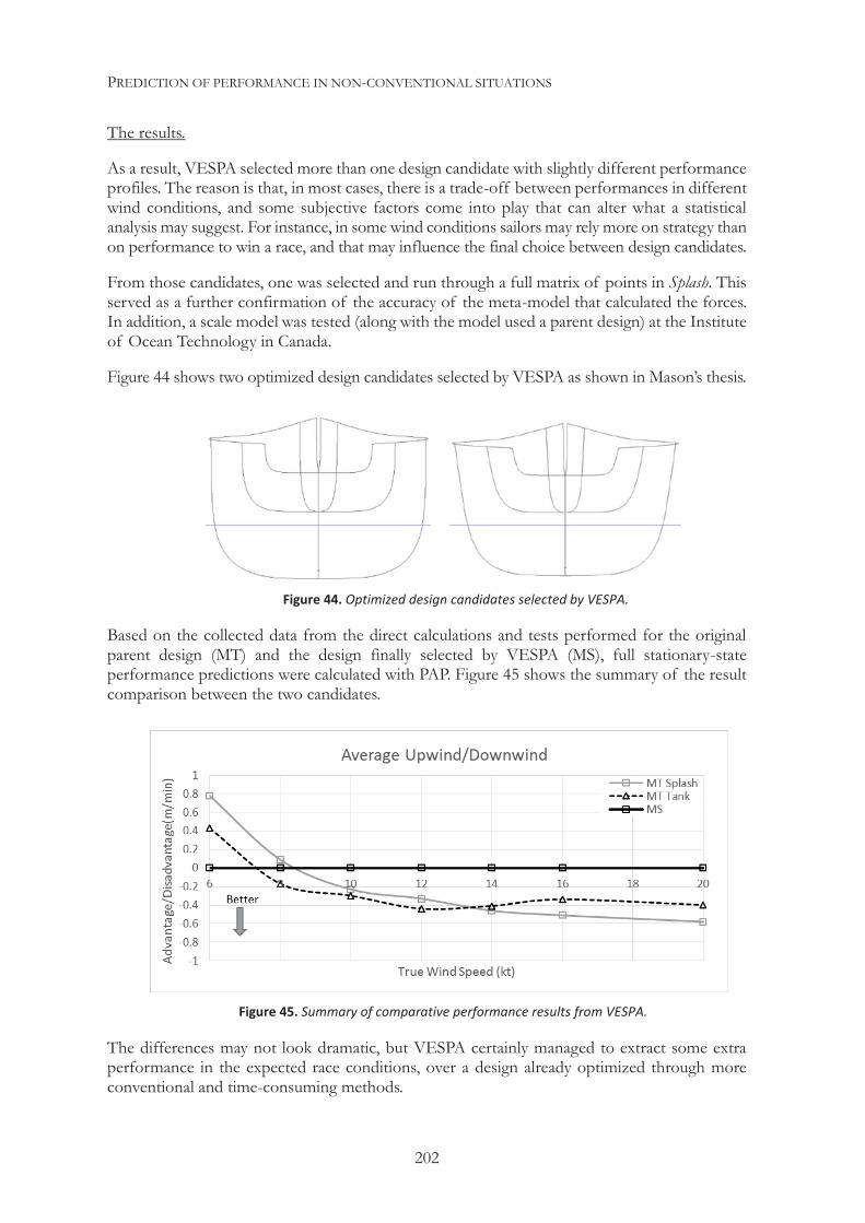
PREDICTION OF PERFORMANCE IN NON-CONVENTIONAL SITUATIONS
202
The results.
As a result, VESPA selected more than one design candidate with slightly different performance profiles. The reason is that, in most cases, there is a trade-off between performances in different wind conditions, and some subjective factors come into play that can alter what a statistical analysis may suggest. For instance, in some wind conditions sailors may rely more on strategy than on performance to win a race, and that may influence the final choice between design candidates.
From those candidates, one was selected and run through a full matrix of points in Splash. This served as a further confirmation of the accuracy of the meta-model that calculated the forces. In addition, a scale model was tested (along with the model used a parent design) at the Institute of Ocean Technology in Canada.
Figure 44 shows two optimized design candidates selected by VESPA as shown in Mason’s thesis.
Based on the collected data from the direct calculations and tests performed for the original parent design (MT) and the design finally selected by VESPA (MS), full stationary-state performance predictions were calculated with PAP. Figure 45 shows the summary of the result comparison between the two candidates.
The differences may not look dramatic, but VESPA certainly managed to extract some extra performance in the expected race conditions, over a design already optimized through more conventional and time-consuming methods.
Figure 44. Optimized design candidates selected by VESPA.
Figure 45. Summary of comparative performance results from VESPA.
A GLOBAL YACHT META-MODEL. THE SAILING YACHT SIMULATOR
203
10| A GLOBAL YACHT META-MODEL. THE SAILING YACHT SIMULATOR
Since the first Chapters, the approach taken towards the performance prediction for sailing yachts has been intentionally gradual. The intention has been to reach a solid understanding of the physics involved in the yacht's behavior, as a first necessary step.
Different components have been introduced and described, ranging from the generated forces to solving techniques, and including discussions on the different parameters, adjustments and constraints involved in the process.
All these components have finally come together to provide the necessary global knowledge and tools required to face the solution of the problem. And it has become obvious that there is a whole range of possible levels of detail in that knowledge, depending on the available information and/or the nature of the analysis to be performed.
Through all this process, the treatment has been as generic as possible, not conditioned by the type of yacht or analysis to be performed (with, for instance, motions being a priori unrestricted). This has become more important as we have moved from the search of a simple optimum stationary-state equilibrium to the more open and complex time-domain analysis.
However, this process, although highly illustrative, does not permit to perform, even a simple analysis until all the components have been put together, as a way to represent reality.
At this point a top-down approach will be proposed, more specifically oriented towards the solution of the problem than towards its description, starting with a simple working structure and progressing down by increasing the levels of detail and accuracy. The idea will be to provide a definition of a full abstraction of the physical reality of the sailing yacht, represented in a global meta-model.
Dynamic effects will also be discussed in more detail. On one hand, this will be done to illustrate the challenge of determining the appropriate level of complexity. On the other hand, the brief discussions made in Chapters 3 and 6 regarding dynamic forces will be expanded beyond the consideration of the yacht as a solid rigid.
Finally, the discussion will steer away from the concept of that global yacht meta-model, towards the connection with its natural interface with reality for the near future: the sailing simulator.
A GLOBAL YACHT META-MODEL Through the previous chapters, the use of models and meta-models have been constant, trying to represent reality in such a way that it can be processed and analyzed with the available knowledge and tools. Both models and meta-models have been used to describe the different parts of the problem, and to provide ways to solve them.
Through this process, although not explicitly, the idea of a virtual yacht has slowly formed. Different components of reality have been replaced by their virtual counterparts:
A GLOBAL YACHT META-MODEL. THE SAILING YACHT SIMULATOR
204
Physical phenomena have been replaced by surrogate models.
Algorithms have been used to generate a continuous amount of data from a discrete set of points.
The sailor’s decisions regarding adjustments have been replaced by constraints and criteria, reflected in the autopilots.
Nature’s balance of forces have been replaced by equilibrium conditions and a relationship between forces and accelerations as per Newton’s laws of movement.
Numerical techniques have been introduced to calculate that equilibrium or the dynamic situation over time.
All these components have been put together with rules managing their interactions.
The description of the structure formed by the different components and rules constitute what we will call the Global Yacht Meta-model.
And it is a meta-model, since it does not represent one specific virtual yacht, but rather describes a generic one. From this generic meta-model, specific instances can be created to define the specific global model for an individual yacht.
This is nothing new but a more precise description of what a VPP ultimately represents: a collection of the knowledge about a yacht used to predict its behavior.
The global meta-model contains different components but two of them are key: the meta-models representing the physical phenomena and the adjustments (along with their management).
Inside those components there are hierarchical levels. Global, higher level aspects are defined and constituted by more specific, lower level ones.
As an example of that, a global model (meta-model) for forces will normally be composed of other lower level models to assess the different components such as drag. Drag in turn will be composed of difference sources, of potential or viscous origin, which can also be associated to different elements of the yacht. Similarly, a simple depowering parameter for the sail plan can be constituted by several settings like traveler position or mainsheet tension, which, ultimately, will combine into a given degree of depowering.
But it is important to observe that the knowledge of that global drag and depowering parameter (along with other equivalent components such as stability, weights, etc.) would already be sufficient to describe the behavior of the yacht, even before investigating the level of detail with which they have been calculated.
This suggests a different perspective on how to solve the problem, putting the emphasis on the global model (as simple as it may be) and progressing gradually down to increase the complexity as required (or possible) in order to improve the accuracy.
The basic idea is that the process itself of understanding the problem should also help to define the required global knowledge and view, the big picture. This will permit to solve it in a more structured and simpler way, in summary more efficiently. It will also increase awareness of the
A GLOBAL YACHT META-MODEL. THE SAILING YACHT SIMULATOR
205
possible relevant issues that could put the process at risk, even if they also appear when going to more detailed levels.
A key advantage of this approach is that a first simple global meta-model can provide a working structure able to produce results. That simple and conceptual global definition does not ignore the complexity of the physical phenomena (forces, motions…) or adjustments, but rather takes simplified representations of them, to offer a basic, yet full, description of the behavior of the sailing yacht, sufficient to feed a simulator that would represent a sailing yacht with a recognizable behavior when sailing.
The next step will be to increase the level of detail and accuracy, and implicitly complexity, as far as required or possible, in order to analyze specific problems related to yacht performance and behavior. This will however be done from a good global understanding regarding what behavior can be expected and how the different components fit together to produce the expected results.
This approach of the problem permits the use of simple models for some phenomena, while still making detailed assessments on others, as long as consistency is preserved. This was already suggested in previous chapters, but starting with a global vision makes this approach more obvious. The stability calculation discussed in section 6.2.4 represents a good example of the generalist approach proposed here.
10.1.1 A SIMPLE META-MODEL AS A STARTING POINT
A basic meta-model, still capable of providing a good description of the behavior of a sailing yacht could be based on:
A yacht constituted as a simple solid rigid.
Known masses, centers of gravity and inertias for each degree of freedom (permitting to estimate hydrostatic and dynamic forces).
Known geometries and volumes (permitting to estimate hydrostatic forces).
Known wind conditions.
A model capable of estimating the basic forces generated by aerodynamic flows (sail plan geometry and a simple sail model).
A model capable of estimating the basic forces generated by hydrodynamic flows (basic lift and drag models for the hull and appendages).
The definition of a simple depowering parameter along with its constraints and optimization criteria.
This simple set can provide the basis for even a detailed performance comparison, for different hull geometries for instance (by just replacing parameters in a detailed hull drag model). More importantly, it is sufficient for describing the yacht behavior in a time-domain analysis with little effort, obviously with all the cautions expressed in previous chapters regarding the implemented models (actually the meta-models used to represent specific phenomena).
A GLOBAL YACHT META-MODEL. THE SAILING YACHT SIMULATOR
206
It is important to remark that this simple meta-model includes a full definition of the structure and rules of the model, even if those are extremely simple. The basic idea is not to define only parts of it, but rather to define the whole system with simple models.
This may not seem very different, but it implies making decisions. For instance, when solving for two degrees of freedom, the other four are not ignored, but rather locked, or the effect of their changes ignored by making a conscious decision. No matter how simplified the set of models is, it is important to assume that they constitute the full, yet simple, definition of the virtual yacht. This permits a structured development of further levels of detail.
In the same way, a simple viscous drag model that calculates forces based on speeds, wetted surfaces and a reference length, is assumed to completely cover (in a simplified way that consciously ignores thickness, lift, shape… etc.) the assessment of viscous forces. However, this model can be improved to account for a much more detailed calculation when considering a more complete definition of the geometries and flows involved.
10.1.2 BUILDING UP IN COMPLEXITY
From the initial basic meta-model described above, it is possible to increase the complexity in the models of the many different phenomena involved when describing the yacht behavior.
This can be done in an almost unlimited way (actually unlimited in a practical sense). And, as it has been stated in previous chapters, the educated common sense of the analyst, based on a good general knowledge of the problem, along with the specific detailed analysis that may need to be performed, will be responsible to set the boundaries.
Most of the detailed aspects in which deeper knowledge may be needed, to address specific problems, have been already discussed. However, the following list intends to provide a non-exhaustive recollection of how the basic meta-model can be gradually completed/improved to provide a richer and more faithful representation of the physical phenomena, and thus, reality:
Consideration of added masses of water (to improve the estimates of accelerations and dynamic forces, something critical for specific studies in highly dynamic situations like maneuverability or seakeeping).
Consideration of the effects of deformations due to the sailing loads.
More accurate force models (based on more detailed descriptions of the geometries and/or of the phenomena involved).
More accurate and/or detailed experimental or numerical data for specific phenomena.
A more detailed definition and consideration of the wind boundary layer in the aerodynamic forces.
Added adjustment parameters for sail plan and/or parts of the yacht (such as movable appendages) with influence on aero and hydrodynamic forces.
Added adjustment parameters for the changes in weights.
A GLOBAL YACHT META-MODEL. THE SAILING YACHT SIMULATOR
207
A multi body dynamic consideration of inertial components due to the movement of specific parts of the yachts created by adjustments.
A consideration of the added flow components due to the movement of specific parts of the yachts due to adjustments.
A detailed management of the sources of power on board for the change of adjustments.
A detailed management of the use of power on board with consideration of the properties of the systems that rely on it.
A more detailed definition of constraints involving the previous aspects.
A more detailed definition of autopilots the management of constraints involving the previous aspects.
From the complexity of the problem we try to describe, it is easy to deduce this list can be extended almost without limit. However, the main idea with this approach is that whichever level of detail is achieved, it should be enough to provide a global representation of the behavior of the yacht, to be expanded as required.
This would be done by providing a basic structure, in which specific emphasis can be put in different components (models, adjustments or autopilots) depending on the type of study or analysis to be performed.
10.1.3 A CODING ANALOGY
The approach proposed in the previous points is not unusual in software design, and as such, programming PASim provided a useful analogy. It was also one of the reasons for looking at the problem with its resolution as the objective, rather than its definition. Something possible, however, from the global understanding of that definition, the “big picture”.
PAP started from a simple steady-state calculation, but it quickly grew, mostly at the lowest level, as more sophisticated and accurate models were incorporated for the estimation of forces, with all other components growing in parallel.
The main problem happened as a result of this “patching” development process. The “heavy” base structure started to constrain and limit significantly the possible analyses that could be performed, or the ways to calculate equilibrium in steady-state solutions, let alone time-domain calculations.
For that reason it was decided to start coding PASim from scratch, although certainly based on the knowledge acquired from PAP, and using many of its components.
But this time, the first working solution started with defining the problems to be solved (in a very open way) and implementing different solvers, working with an undetermined number of decision/optimization variables and degrees of freedom.
The initial problem implemented was the simplest problem defined in Chapter 6, but procedures were provided to perform less restrictive calculations from the first moment.
A GLOBAL YACHT META-MODEL. THE SAILING YACHT SIMULATOR
208
Before progressing down in complexity, simple models were implemented so full six degrees of freedom could be run, as well as time-domain analyses based on a simple solid rigid without added masses. Moreover, this process could be managed by an automation module, initially simple, and provided a basic but sufficient user interface. The key structures were finally in place with no compromises or restrictions.
From that moment on, detail and complexity started to increase, but this time, over a solid, simple and well structured framework.
The main consequence has been to significantly facilitate the expansion of the program, with new additions not requiring adjusting all the existing capabilities, but rather expanding them. The key to achieve this was to start defining the global meta-model of this computational tool from the knowledge of what the main components were and how they should interact.
A MULTIBODY DYNAMIC SIMULATION One of the areas listed in the previous point for adding levels of complexity to the basic meta-model was a better consideration of the dynamic effects. The references to this topic during the discussion about the generation of forces have been intentionally limited to a solid rigid at first. This is the classical approach to dynamic simulation for sailing yachts, and it is perfectly valid in most cases when looking for a steady-state solution it is common to carry that simplicity to time-domain calculations. However, it may be insufficient for a number of analyses.
Then, a first complication was introduced: the modifiers that take into consideration the effects of deformations, in those cases when they could have a non-insignificant impact on the generation of forces (as is the case with the platform twist in multihulls).
The second complication came when some of the possible adjustments had a significant effect on weights and centers of gravity. This was obvious when the adjustments were intended to manage ballast. However, in some cases, indirect effects were present, like for instance, when moving lifting boards. This was a situation in which the changes in weights (centers of gravity) and immersed volumes, a side effect of the adjustment (the purpose of which was to act on forces of hydrodynamic origin), had an importance that needed to be taken into consideration.
This was a clear hint suggesting that fundamentally, in time-domain calculations, there were situations that involved multibody dynamics, adding a layer of complexity to the problem.
We will discuss this in more detail, since it adds some necessary level of detail to our meta-model. But also, because introducing a global view to the dynamic component, provides a perfect example of how complex an analysis can get, and how necessary it is to define reasonable limitations to that complexity. Once again, educated common sense is required, and using it permits to approach problems that, otherwise, would be difficult to solve.
Multibody Simulation (MBS) could be described as a numerical simulation in which multibody systems can be composed of various rigid or elastic bodies, whether they are solids or even fluids. These bodies have their connections modeled with kinematic constraints (such as joints) or force elements (such as levers, springs, dampers…). Friction forces can be modeled as well.
A significant part of the simulation involves the definition of the interactions between the different parts, which include the use of collision algorithms, to determine when and how the
A GLOBAL YACHT META-MODEL. THE SAILING YACHT SIMULATOR
209
interaction happens. This type of simulation is the adequate tool to conduct motion analyses in complex systems that involve multiple components.
A sailing yacht, considered as a whole, is a complex system that evolves following different paths in every variable involved. The most obvious one is the geographical path, defined by the X and Y coordinates of a fixed “world” system of reference. However, the same happens in non-geographically related variables when outside of a stationary-state equilibrium situation, that is the case through most real sailing.
This implies that a number of adjustments are constantly made, that have a direct impact on the generated aerodynamic, hydrodynamic, gravitational and hydrostatic forces. However, it is possible to move up in the chain to identify how those adjustments are performed. This involves the mechanisms that make them possible, as well as the origin of the power required to actuate those mechanisms.
Ultimately, it will go to the source of power, in most cases the sailors that perform the adjustments.
A very detailed calculation can be made, which includes all the elements involved in the process, whether they are mechanic, hydraulic or electric (or even magnetic, chemical, etc.) down to the simplest individual component.
For this purpose, there are a number of packages in the market for multibody dynamic simulation that cover many different types of problems. Amongst them, “Adams” (64) is probably the best known package, and one of the oldest in this field. However, other solutions are available, including open source initiatives like “MBDyn” (65) and MBS3D (66), as well as other commercial solutions like “COMSOL Multiphysics” or “RecurDyn”, that are appearing to face the increasing demand for this type of simulations. “Simulink” (67) is an environment for model simulation that works inside “Matlab” and that is quickly gaining popularity to model and simulate dynamic systems.
10.2.1 A RATIONAL APPROACH TO DYNAMIC SIMULATION
As a consequence of what was described before, it would be tempting to consider modeling every detail in the complex dynamic process of a yacht while sailing. However, that would guarantee failure to achieve the objective of having a global working model.
A top down approach starting from an extremely simple model, and then progressing in complexity, is always a better approach. One of the main reasons is that it provides an initial working solution against which to benchmark further progress, when adding more detail.
The simple answer in terms of defining the level of detail is to go as far as it provides visible benefits, but not any further. Considering an absurd example, performing a global multibody simulation including the components of a sailor’s body, even if it were possible, would require unlimited resources for a minimal benefit towards describing the dynamic behavior of a yacht.
However, it is not hard to model a sailor like a system described by its own behavior in terms of inputs/outputs (which eventually will be the only relevant area when performing activities in the yacht). This could include the definition of aspects as detailed as:
Which are the power delivery specifications (including maximum available power vs. time for different uses of that power, effects of recovery etc.)
A GLOBAL YACHT META-MODEL. THE SAILING YACHT SIMULATOR
210
Whether the sailor can perform other tasks, and whether these interfere with the generation of power.
Whether a specific position on the yacht is required for any of the tasks.
Possible movement paths and speeds on board, including collision detection with other sailors or elements on the yacht.
Dependencies of any of the tasks on the status of other sailors or yacht elements.
Weight of the sailor and its effects as a function of position and motions.
Windage of the sailor and its effects as a function of position and motions.
That is a complex yet feasible definition of a sailor, which can also be replaced by a simple power delivery curve and basic weight/position considerations (and it usually will be).
A winch can provide another example of unnecessary complication to be avoided. In order to model its role in a yacht, just including in the global model information about transmission ratios, losses for different speeds and amounts of delivered power, exceeds the normal treatment given to a simple (yet important) mechanical component.
Needless to say, a winch manufacturer will study in detail the interaction between the internal moving parts, as an ergonomics study will look at how individual parts of the human body will interact with said winch. However, a rational approach to the dynamic definition of a yacht as a multibody system needs to establish reasonable limits in terms of required levels of detail.
But there are benefits to understanding how to evaluate the interaction with at least some of the adjustments in a yacht. For example, the different controls of a wing sail or an adjustable lifting board are going to require different amounts of power depending on a number of external factors.
Different elements offer distinctive challenges in creating a valid input/output model. These challenges can range from mechanical or frictional problems, with strong dependencies on speeds and forces, to, for instance, a hydraulic system in which additional factors related to the available power may become a significant constraint.
However, even when kept at a very simple level, proper definition of the main interactions between the different elements and their ultimate drivers (generators of power) will help to assess the feasibility of possible actions in highly dynamic situations. In the case of actions with impact on weights or immersed volumes, as well as on the generated hydro and aerodynamic forces, taking into account the interactions will help to provide a simple and direct path towards a full consideration of their effects on the yacht motions and performance.
A SAILING SIMULATOR Sailing at high level has become a much more technical activity than it was only a few years ago.
One of the reasons is the advent of significantly more complex sailing machines with an almost unlimited number of possible adjustments. Another reason is the increasingly competitive environment, in which the smallest difference in boat handling can provide the small edge necessary to defeat the adversary.
A GLOBAL YACHT META-MODEL. THE SAILING YACHT SIMULATOR
211
This situation has forced high performance sailors and designers to work more closely together than ever. The sailors can benefit from a better technical and scientific understanding of what is happening on board. This helps to make the yachts perform at their best in normal conditions, but also improves the chances of having rational (in terms of performance or safety) reactions in unexpected situations. Designers, on the other side, have access to much better design tools and sailing data, but can also greatly benefit from the subjective opinion of technically savvy sailors.
There is an additional factor that, to some point, is unique to sailing. The environmental conditions in which sailing takes place are constantly changing. This makes the ocean an incredibly complicated laboratory for extracting performance information for sailing yachts, and makes this process a very time-consuming activity, often with the expectation of an uncertain outcome.
All these factors, along with a number of added benefits that will be briefly discussed later, make the idea of a proper physical sailing simulator very attractive, and it is certainly a technical challenge, but within reach.
A number of simplified alternatives have been tested with dinghies, but with a less technical purpose than the one we will propose, and certainly with a much lower level of complication and reality.
In this chapter, we will propose a schematic approach and specification for a general-purpose sailing simulator, as an implementation of the global yacht meta-model proposed before. This will provide a link between said global yacht meta-model and a simulated physical reality with the aim of reproducing in a faithful way the actual physical reality. This can be applied to different types of yachts and navigation, bringing a significant number of potential uses and benefits.
10.3.1 THE OBJECTIVE
The main objective in this chapter is to provide a basic definition and specification of a sailing yacht simulator that will provide an interface for the sailors with the modeled virtual yacht, based on the technical knowledge available about it.
This virtual yacht may be just a design with no physical existence of an actual yacht. The only requirement is to have available the models and rules required to describe its behavior with an accuracy corresponding to the purpose of the simulation.
In order to resemble reality, the simulator must provide sufficient input to the sailor’s senses so that the experience would be immersive enough to provide a realistic environment. This would necessarily provide an accurate feedback to the sailor’s actions, ideally reproducing faithfully those that could be expected in reality.
A number of senses are involved in the full sailing experience, but clearly, the most relevant are sight and touch, with some influence of hearing. Hearing plays an interesting role: while the sound is not a vital part of the reality that the sailor experiences (although it is not completely irrelevant), the ear plays a key role in equilibrium.
Based on that, a sailor operating the simulator should:
A GLOBAL YACHT META-MODEL. THE SAILING YACHT SIMULATOR
212
Be able to feel the movements of the yacht, whether they are a consequence of his own actions, changes in the environmental conditions, or created situations.
Be able to observe his surroundings as an additional input to evaluate his situation related to position, adjustments, environment, etc.
Receive information equivalent to the one he would obtain from the usual onboard electronics.
Receive additional information, to be defined and evaluated.
These requirements have an obvious impact on how the simulator must be designed and operated, and from the technical point of view will require:
A moving platform capable of reproducing the different positions and accelerations that the sailors would experience while sailing.
A Virtual Reality (VR) environment capable of providing the sailors with an accurate perception of the yacht attitude, motions and situation of adjustments (or their consequences).
A time-domain analysis software engine to calculate the yacht behavior based on the environmental conditions, the definition of the yacht and the effects of the actions carried out by the sailors.
A Race Modelling Program (RMP), directly connected to the software engine, and intended to model actual racing situations, modelling courses, wind changes and interaction with other competitors.
Interfaces to turn the calculated situations of the yacht into the motions and visual situations provided to the sailor.
Interfaces to turn the sailors’ actions into the adjustments that the software engine will use for its calculations.
All these working elements would be responsible to provide a sailing experience that should, on one hand, be as close as possible to the perceived reality of the sailors, and on the other hand, respond to a realistic model of the actual behavior of the yacht. The objective in terms of perceptions is to make the virtual experience a recognizable experience of reality.
10.3.2 THE PHYSICAL PLATFORM
Motions are inherent to sailing. They constitute a significant part of the sailor’s perception of the yacht behavior. A good example of this is how blind sailors can sail with a good “feeling” of the yacht’s attitude or even the much more common situation when sailing in the dark at night.
The position of the yacht informs the sailor about the current condition (heel related to a sail setting or wind strength, or pitch related to the position on board or boatspeed). The perceived
A GLOBAL YACHT META-MODEL. THE SAILING YACHT SIMULATOR
213
added accelerations provide the necessary feedback regarding changes in environmental conditions and setting.
The first impression would probably be that both sources of perceptions, position and accelerations, need to be modeled. However, the fact that gravity is the main and always present source of accelerations suggests that it may be enough to reproduce the resultant of all the accelerations.
In absence of visual references, accelerations are the factor that drives subjective perceptions regarding both positions and motions. The human body perceives equilibrium through accelerations. Even in a static position, the direction of the acceleration of gravity will determine the perceptions about inclinations from the vertical. Since the visual perceptions of the user of the simulator are to be provided by a virtual reality system, what matters is the sum of accelerations that will be perceived and not the position itself (although that position will provide the gravitational input of the accelerations).
In an analogy to the generation of apparent wind, it will be the global apparent acceleration, along with the virtual visual perception that will determine the sum of position and dynamic accelerations. That is the reason why both the dynamic and the static (due to gravity) components of that acceleration will need to be provided to the user (with the help of the always-present gravity).
This way, it is possible to add a perception of acceleration in one direction by just inclining a platform in the opposite direction, especially when using small angles (where the cosine is close to one). The cosine of the angle will remain close to one, but the sine will generate the horizontal component (in the visually perceived horizontal plane of the user) required to experience that longitudinal acceleration.
This is taken into account when designing a system for the required range of positions and accelerations to be reproduced, trying to reduce them into accelerations. A static platform will be providing a unique acceleration in the Z-axis, corresponding to the acceleration of gravity. From that, the rest of the effects simply add up.
The basic platform
A number of possibilities are available and have been experimented, but the “Stewart Platform”, also known as Synergistic, or more commonly Hexapod, has been without discussion the preferred choice for motion simulation. E. Gough started using the six-jack layout platform in 1954, and D. Stewart published his paper describing it (68) in 1965.
It is basically a parallel robot incorporating six prismatic actuators. These actuators are mounted in pairs to the mechanism's base, crossing over to three mounting points on a top plate. Each actuator is individually controlled and driven and the combination of all of their movements permits to move the top plate in the full six degrees of freedom. That is the reason why these devices are also called “six degrees” platforms.
As a parallel robot, the Stewart platform does not include the high quality (and weight) rotary joints that serial robots require, making it a significantly lighter solution. For this reason, it allows the addition of significant weights to the top platform, making it the ideal candidate for positioning large masses with high precision (as happens with electrostatic or magnetic lenses).
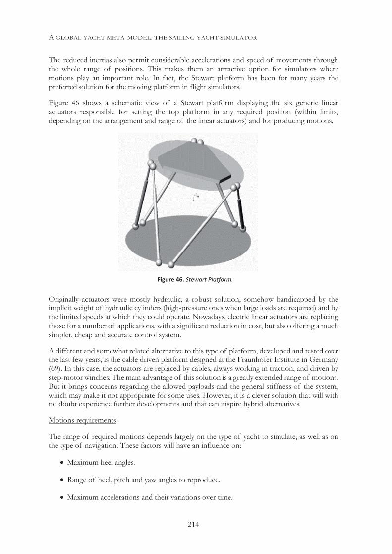
A GLOBAL YACHT META-MODEL. THE SAILING YACHT SIMULATOR
214
The reduced inertias also permit considerable accelerations and speed of movements through the whole range of positions. This makes them an attractive option for simulators where motions play an important role. In fact, the Stewart platform has been for many years the preferred solution for the moving platform in flight simulators.
Figure 46 shows a schematic view of a Stewart platform displaying the six generic linear actuators responsible for setting the top platform in any required position (within limits, depending on the arrangement and range of the linear actuators) and for producing motions.
Originally actuators were mostly hydraulic, a robust solution, somehow handicapped by the implicit weight of hydraulic cylinders (high-pressure ones when large loads are required) and by the limited speeds at which they could operate. Nowadays, electric linear actuators are replacing those for a number of applications, with a significant reduction in cost, but also offering a much simpler, cheap and accurate control system.
A different and somewhat related alternative to this type of platform, developed and tested over the last few years, is the cable driven platform designed at the Fraunhofer Institute in Germany (69). In this case, the actuators are replaced by cables, always working in traction, and driven by step-motor winches. The main advantage of this solution is a greatly extended range of motions. But it brings concerns regarding the allowed payloads and the general stiffness of the system, which may make it not appropriate for some uses. However, it is a clever solution that will with no doubt experience further developments and that can inspire hybrid alternatives.
Motions requirements
The range of required motions depends largely on the type of yacht to simulate, as well as on the type of navigation. These factors will have an influence on:
Maximum heel angles.
Range of heel, pitch and yaw angles to reproduce.
Maximum accelerations and their variations over time.
Figure 46. Stewart Platform.
A GLOBAL YACHT META-MODEL. THE SAILING YACHT SIMULATOR
215
These factors will condition the design of the platform, but also the range of situations that can be realistically reproduced by a given system.
At this point, we will talk about a generic platform, since it can be constituted either by a single Stewart platform or by a more complex system. This can be driven, for instance, by a requirement of having a large range of variation for heel angles, maybe to both tacks (if tacking or gybing need to be reproduced). Stewart platform maximum changes in angles vary, but 20 degrees are a common limit. Considering that heel is a constant in most sailing modes, it may be advisable to provide a separate platform for that single degree of freedom, on top of which a Stewart platform would deal with the rest of motions.
The same can apply for other degrees of freedom. However, it is clear that the Stewart platform remains as the main element of the part of the simulator related to positions and accelerations, and the type of use of the simulator amongst the many possible configurations will condition the design of the global platform.
10.3.3 VIRTUAL REALITY ENVIRONMENT
The concept of “presence” is at the core of simulators and represents the main objective of the Virtual Reality (VR) environment, led by the media, computer and gaming worlds since their
initial steps. M. Lombard and T. Ditton discuss this concept with a broad perspective in an article (70) in which the concept is explored from many different points of view, most of them considering the user as a spectator, but not limited to that.
One of the discussions focuses on the fact that the user sees his task performance affected by his perception of reality, and in a simulator this effect, even if inside the virtual environment, needs to be taken into consideration. A number of additional effects and benefits affecting memory, skill training, desensitization (to distracting factors) etc., are also discussed amongst many other in the article, which is an excellent reference regarding presence and perceptions.
Thus, it is hard to ignore that a simulation would not be complete without providing a visual interface, necessary to add up to the normal perceptions of the sailors. Actually, in some experiments with moving platforms, the lack of a consistent visual feedback is sometimes a cause for motion sickness beyond what could be expected from a trained sailor.
But beyond this, the visual input is key for the sailors. Whether it is a helmsman steering through the race course or a sail trimmer adjusting the shape of a sail, the use of the visual feedback is constant in the real world and needs to be reproduced as accurately as possible in the virtual world.
One of the keys of the VR environment is the visual interface, and the recent developments have brought to the general public solutions, that could only be dreamt only a few years ago. Oculus Rift (71) leads this field, but recent arrivals like the HTC Vive (72) interface, or the coming Sony Morpheus (73) are providing the hardware components necessary to implement the visual interface. All these solutions also offer development kits to facilitate their integration with different software.
These devices display in an immersive way the images created by the VR environment software engine. However, they also detect the user movements and provide this engine with the position and orientation of the user so that the correct view corresponding to those can be displayed. For instance, a sail trimmer tilting his head to watch the top of his mainsail will see this part of

A GLOBAL YACHT META-MODEL. THE SAILING YACHT SIMULATOR
216
the sail displayed, as he could expect in the “real world”. Figure 47 shows one of these devices, in this case the Oculus Rift.
The other key component is the software side, which is responsible for providing the images to be visualized to the interface. These images should include information regarding:
The surrounding environment, with geographical landmarks (when they are available and relevant to sailing), and ideally a representation of the current wind and waves conditions on the water surface.
The yacht position relative to the water, including its attitude and any indication of the speed (such as a wake, for instance).
The current situation of any sailing adjustments that may be visually identified (such as the trim state of a sail or wing, or the position of a lifting board).
The normal information provided by the yacht’s onboard electronics.
Any added information of interest.
Any other yacht in case the simulation involves any rivals, such as a visual indication of their positions and motion state.
Some initiatives have produced this environment, from video games to media support tools to facilitate the spectator experience on TV, but for a simulator the requirements are stronger as perceptions play a more important role.
One of them is A Mason’s VIRTAC (74), discussed in some detail in two articles published in Seahorse Magazine (75). This system provides the software component to connect the VR interface to different sources of data, ranging from actual sailing data to that generated by the VPP time-domain analysis. In this last process, the VPP provides a reduced set of data to the
Figure 47. Virtual Reality Interface.
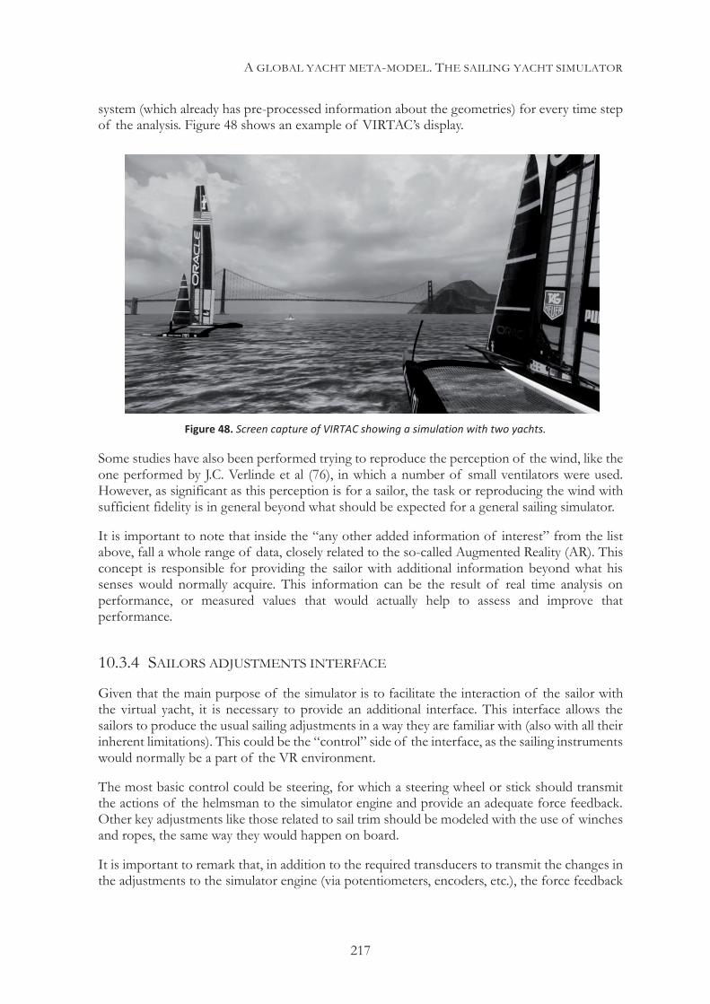
A GLOBAL YACHT META-MODEL. THE SAILING YACHT SIMULATOR
217
system (which already has pre-processed information about the geometries) for every time step of the analysis. Figure 48 shows an example of VIRTAC’s display.
Some studies have also been performed trying to reproduce the perception of the wind, like the one performed by J.C. Verlinde et al (76), in which a number of small ventilators were used. However, as significant as this perception is for a sailor, the task or reproducing the wind with sufficient fidelity is in general beyond what should be expected for a general sailing simulator.
It is important to note that inside the “any other added information of interest” from the list above, fall a whole range of data, closely related to the so-called Augmented Reality (AR). This concept is responsible for providing the sailor with additional information beyond what his
senses would normally acquire. This information can be the result of real time analysis on performance, or measured values that would actually help to assess and improve that performance.
10.3.4 SAILORS ADJUSTMENTS INTERFACE
Given that the main purpose of the simulator is to facilitate the interaction of the sailor with the virtual yacht, it is necessary to provide an additional interface. This interface allows the sailors to produce the usual sailing adjustments in a way they are familiar with (also with all their inherent limitations). This could be the “control” side of the interface, as the sailing instruments would normally be a part of the VR environment.
The most basic control could be steering, for which a steering wheel or stick should transmit the actions of the helmsman to the simulator engine and provide an adequate force feedback. Other key adjustments like those related to sail trim should be modeled with the use of winches and ropes, the same way they would happen on board.
It is important to remark that, in addition to the required transducers to transmit the changes in the adjustments to the simulator engine (via potentiometers, encoders, etc.), the force feedback
Figure 48. Screen capture of VIRTAC showing a simulation with two yachts.
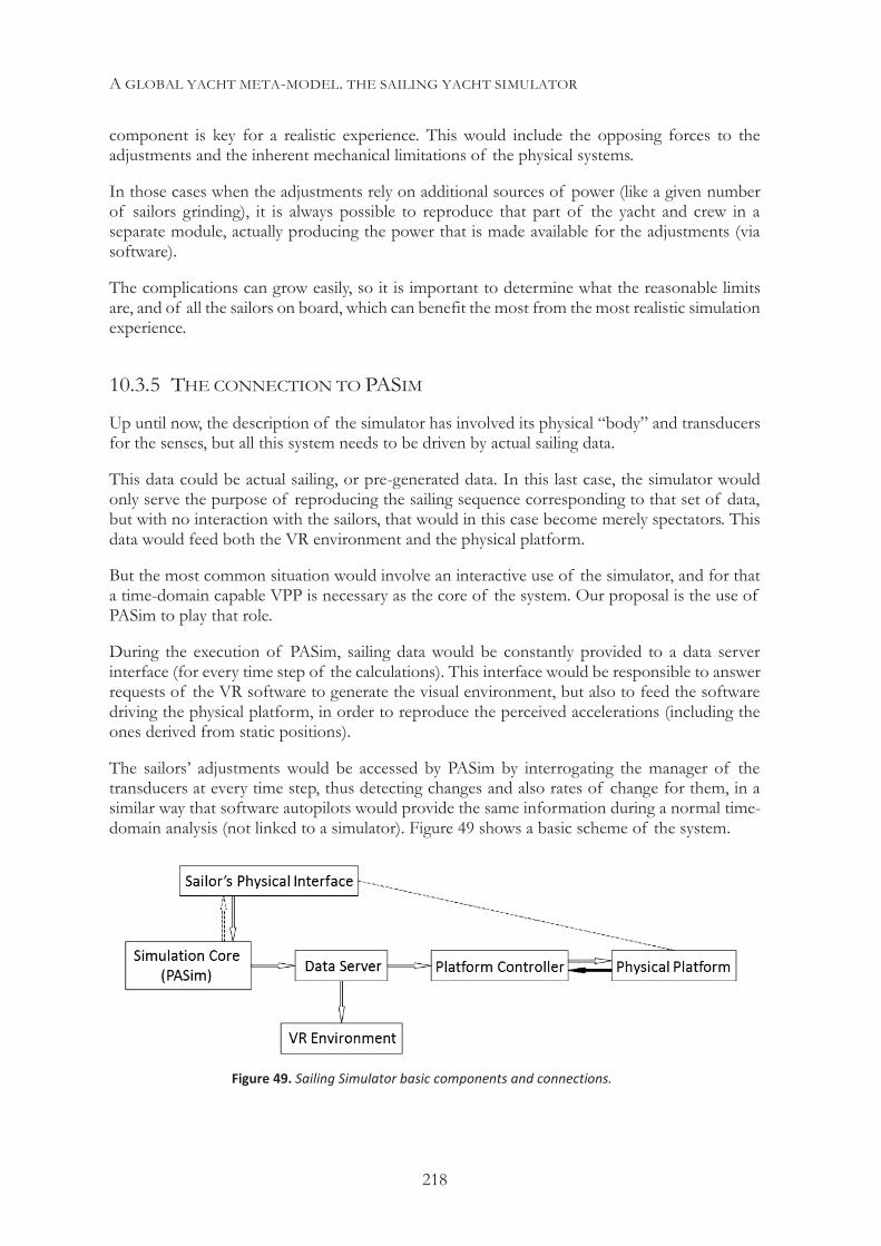
A GLOBAL YACHT META-MODEL. THE SAILING YACHT SIMULATOR
218
component is key for a realistic experience. This would include the opposing forces to the adjustments and the inherent mechanical limitations of the physical systems.
In those cases when the adjustments rely on additional sources of power (like a given number of sailors grinding), it is always possible to reproduce that part of the yacht and crew in a separate module, actually producing the power that is made available for the adjustments (via software).
The complications can grow easily, so it is important to determine what the reasonable limits are, and of all the sailors on board, which can benefit the most from the most realistic simulation experience.
10.3.5 THE CONNECTION TO PASIM
Up until now, the description of the simulator has involved its physical “body” and transducers for the senses, but all this system needs to be driven by actual sailing data.
This data could be actual sailing, or pre-generated data. In this last case, the simulator would only serve the purpose of reproducing the sailing sequence corresponding to that set of data, but with no interaction with the sailors, that would in this case become merely spectators. This data would feed both the VR environment and the physical platform.
But the most common situation would involve an interactive use of the simulator, and for that a time-domain capable VPP is necessary as the core of the system. Our proposal is the use of PASim to play that role.
During the execution of PASim, sailing data would be constantly provided to a data server interface (for every time step of the calculations). This interface would be responsible to answer requests of the VR software to generate the visual environment, but also to feed the software driving the physical platform, in order to reproduce the perceived accelerations (including the ones derived from static positions).
The sailors’ adjustments would be accessed by PASim by interrogating the manager of the transducers at every time step, thus detecting changes and also rates of change for them, in a similar way that software autopilots would provide the same information during a normal time-domain analysis (not linked to a simulator). Figure 49 shows a basic scheme of the system.
Figure 49. Sailing Simulator basic components and connections.
A GLOBAL YACHT META-MODEL. THE SAILING YACHT SIMULATOR
219
Without getting into details, no specific developments are necessary, as all the required components for the connections between the different elements are easily available.
It is important to note that for a proper representation of reality, the delay between actions and effects must be similar to the one that exists in reality. This is not a problem in the calculations and visual representations (although it was just a few years ago), but the moving platform suffers from inertial effects that can complicate the situation.
Fortunately, the real yacht also suffers from these effects, and this can generate delays in the motion reactions. The key is to match the real situation, and for that, there are solutions that help the platform controller, such as supplying to the platform controller the forces and moments that generate the motions along with the inertial properties of the yacht. Then, the platform controller could compare them to the inertial properties of the platform, and an adequate algorithm could benefit from additional resources to match the real motions, in phase with the changes in the sailing conditions.
It is important to point out that the perceived accelerations due to angular motions are dependent on the position of the sailor on the yacht. This is important when determining which accelerations he will be subject to, and it requires a definition of the position. However, there are cases were that position can change, as it would be the case in a dinghy. In this situation, the position of the sailor should be tracked, to correct the boat’s inertia, but also to define the accelerations that the sailor is subject to.
10.3.6 USES AND BENEFITS
The possibility of having a physical simulator, capable of reproducing in a reasonably accurate way the interaction between the yacht, elements and sailors, opens a world of possibilities in the communication between designers and sailors. And this is fundamental in high performance projects, since performance ultimately depends on more factors than just a “potentially fast” design and a talented sailor.
Maximizing performance in a changing environment, or steering course with the purpose of defeating other yachts, require constant adjustments. These adjustments need to happen in a simultaneous way with everything else that happens on board, from generating power to evaluating conditions in order to take a tactical or even performance decision.
With this in mind, a sailing simulator may not have its main role as a design tool in the traditional sense (the embedded VPP in the simulator core would already play that role), but it still provides support regarding the difficulties related to achieving that theoretical maximum performance. However, it provides an incredibly powerful tool to acquaint sailors with the technical nature of the sailing yachts.
There is a wide range of potential uses for a sailing simulator, and associated benefits, most of which will require a representation of reality as faithful as possible. The next paragraphs provide a non-exhaustive list of the potential uses. This list will, without any doubt, grow with its use.
Assistance towards a steeper learning curve for the sailors
The simulator provides a platform that intends to reproduce the behavior of the yacht, but in addition, it also gives the sailors an immediate feedback. This allows a quick measurable
A GLOBAL YACHT META-MODEL. THE SAILING YACHT SIMULATOR
220
evaluation of relationship between actions and effects, with a measure of performance, that will with no doubt help a rapid progress towards the understanding of the yacht.
Training of natural reactions
Changes can be consistently repeated and the effect of reactions evaluated. By a trial and error process, the normal correct reactions from the sailors can be trained to favor reactions promoting performance or maintaining safety.
Evaluation of optimal responses to soft transitions and patterns of changes
Although a VPP can analyze and provide suggestions for an optimal management of transitions through actions and adjustments, those need to be executed within normal reaction times. A realistic environment would allow testing suggested adjustments, or leave to the sailor the search for the intuitively best solution, which at that time can be properly evaluated.
Evaluation of situations with similar performance but different executions
Sometimes there are different sets of adjustments or changes that provide a similar performance output but through different actions. The possibility to let the sailors experiment with them, and to select those that they feel more comfortable with in realistic conditions, maximizes the chances to sail the yacht at maximum performance most of the time.
Training of the interaction between sailors through transitions
Normal interactions between sailors, like for instance between a helmsman and a mainsail or wing trimmer, can be tested. Maneuvers that require coordinated actions between them (or most of them) can be trained.
Training anticipation regarding what to expect from unusual situations
Unusual situations can be evaluated without danger, facilitating the analysis of “what if ” scenarios.
No dependency on weather conditions
Environmental conditions can be arbitrarily set and changed, unlike in nature. This provides and invaluable base for high productivity tests.
Training of subsequent on-the-water tests
On-the-water tests are time-consuming and difficult to interpret, often requiring evaluations which are hard to perform in real time. The simulator would permit to practice those tests and anticipate expectations or measures of merit. This would have a significant impact on reducing the number of tests that must be discarded after a test session, and would build a roadmap for the day depending on intermediate results.
Evaluate safety limits and corrections
Although the models used and the physical platform would not normally cover extreme situations such as capsize, the simulation engine can anticipate how close to the limit the yacht can be. This tool would permit to evaluate possible reactions to correct situations before they are out of control, and educate perceptions.
A GLOBAL YACHT META-MODEL. THE SAILING YACHT SIMULATOR
221
Anticipate the behavior of a new design or type of yacht
New designs or new types of yachts are always a challenge, especially when they suppose a departure from the comfort zone of a sailor. A realistic simulator would provide a base to educate the perceptions of the sailors. It will also teach them the specific characteristics and reactions of a yacht or type of sailing they are not familiar with.
Model racing situations
Through the use of recorded data and/or under the management of a race modelling program (RMP), it is possible to evaluate racing situations, involving wind changes, but also the presence of opponents. The interaction with those opponents would be modeled by the RMP in order to test realistic “what if ” situations under varying wind conditions.
Test deck gear
The design of deck layouts and hardware positioning takes into account different factors. The ergonomic aspects are also influenced by kinetic and kinematic effects, which should be considered. Actual accelerations and motions can be reproduced in a simulator, and help to optimize the efficiency of the deck systems in realistic situations, facilitating the interaction with the sailors.
Provide a test platform for Augmented Reality
Augmented Reality has been briefly mentioned before but it will become a key factor when sailing high performance yachts. It has happened, to some level, since navigation instruments and on-board electronics started to provide more information than the bare senses of the sailors could perceive.
Today the amount of measured data has increased dramatically, but also, a significant part of that data is processed in real time and becomes available to the sailors while they are navigating. This creates a problem, since the reception of the information enters in conflict with the normal perceptions, communications on board, and even just the internal processing of all that information in order to take constant decisions.
An almost infinite number of strategies can be tested in order to select and supply the right information, at the right time, with a minimum disruption to the sailor’s activity. Testing on the water every one of the large number of possible alternatives would be time consuming and, to some point, disruptive inside a general testing program.
The sailing simulator becomes a perfect tool to perform those tests, with the added possibility of directly measuring the effect of the supplied information and the way it is delivered.

A GLOBAL YACHT META-MODEL. THE SAILING YACHT SIMULATOR
222
This page intentionally left blank
CONCLUSIONS
223
11| CONCLUSIONS This thesis had the aim of providing a general framework and, more importantly, a structure of thought to understand the behavior of a sailing yacht as a prerequisite to properly assess its performance.
Unlike in the approach of the classical velocity prediction programs (VPP), the main focus has not been put on the supporting models, but on the structure itself, moving to the detailed calculation of the forces once a generic approach was in place.
This process started with putting together the different factors involved in the equilibrium of the yacht, describing their interactions and (along the way) defining the relevant aspects that rule the behavior of the yacht.
Then, different strategies to obtain data from different origins regarding the forces involved were discussed, proposing a methodology the collection, analysis and treatment of that data, which also involved the design of the experiments necessary to achieve that objective.
Through all that process a significant emphasis was put on the importance of a good global knowledge of the problem in order to provide a general vision. This would support the definition of the engineering “common sense”, necessary to make practical decisions and protect the accuracy of the process itself.
After that, the process of performing different analyses was studied, raising awareness about some potential problems and proposing procedures and solutions to efficiently obtain useful results, for which some critical criteria were also provided.
Different examples illustrated then the most significant topics discussed in the previous chapters.
During the whole process, an intentionally general approach has been maintained that departs from the classic approach to performance prediction for sailing yacht. A complete freedom has always been assumed for the yacht motions and adjustments, only dependent on the laws of physics or the rules defining the type of analysis to be performed. The different approach for the calculation of stability described in section 6.2.4 constituted a good example of how to look in a different way at one of the most traditional analysis performed in naval architecture.
This general approach permitted to put together an open structure composed of different elements to calculate forces, define interactions and calculate solutions. This structure, independent from the design to be analyzed or the type of analysis itself, is completed with the set of rules that control the interaction of the different elements. It constitutes what we have defined as a global meta-model of the sailing yacht.
This is not an added element but rather the recognition of the definition of this structure as an entity itself, which represents a virtual yacht, acting as a proxy of the real one.
An immediate consequence was the implementation of the structure (the meta-model), into a computational tool, PASim, intended to assess performance for a broad range of yachts or types of analyses, as its core concept intends to do.
CONCLUSIONS
224
Finally, a connection with reality is proposed by using a sailing simulator, providing an interface between the abstract calculations and the concrete perceptions of the sailors, as a way to facilitate the technical connection between designers and sailors, both from scientific and sporting points of view.
Critical assessment and contribution
Sailing yachts have evolved significantly over the years and, especially in the last decades, new design and way of sailing have appeared creating difficulties for its analysis with conventional tools. A good example of this are fully-foiling yachts, but even simple multihulls or dinghies subject to seriously dynamic conditions challenge the classic methods for assessing their performance.
Equilibrium situations that were assumed in the past cannot be taken for granted anymore and there is a constant change in the way forces are generated, the elements used for it, and consequently, the types of analyses that engineers may be interested in performing. Those are the reasons that drove the desire to use this general approach, with a structure simple and capable enough to adapt to this multiplicity of situations.
Additionally, there is an increasing trend to strengthen the link between sailors and designers. Providing a common platform to facilitate the understanding of the physical problems involved in sailing is a significant step in that direction.
The whole process to reach that point has brought up a number of topics that were not common in traditional performance prediction and has introduced some innovative solutions. Amongst them, we can highlight:
The consideration of the full six degrees of freedom for the yacht motions as a starting point, also taking into account the dynamics of the different elements that constitute the yacht, and their interactions.
The possibility to use multiple adjustments, having continuous control over them, both for a stationary-state calculation or a time-domain analysis.
The introduction of autopilots as criteria for the management of those adjustments. Autopilots are a key component of the time-domain analysis but, as it was shown in the examples, they can also play a significant role in steady-state calculations in more complex situations.
A methodology to design experiments to obtain numerical and experimental data, along with procedures for acquiring it, including precautions to guarantee its quality and accuracy.
Proposed procedures to use the collected data to generate models for the calculation of forces, providing a continuous output through the area of interest of the parametric space. This includes the generation of “virtual” data points in order to improve the robustness of the model.
The basic principles of a method to derive “virtual” data from a reduced number of points, using a much denser but topologically similar set of data.
A number of innovative uses have also been suggested and demonstrated, through some of the examples described in Chapters 8 and 9.
CONCLUSIONS
225
Some potential disadvantages of this approach.
The general approach here proposed is not exempt from potential weaknesses, when compared to other ways to face the problem of the behavior of sailing yachts. However, this author believes that the benefits exceed the possible drawbacks.
In the case of specific problems, a particular approach may be able to provide a more robust and computationally efficient calculation. On the other hand, the constant increase in computational power has been reducing those potential benefits, while the limitations of the specific approaches remain intact.
Also, the usefulness of a general tool for solving specialized problems is conditioned by the models that sustain it, and this at first may appear as a limitation, when compared with specific codes and techniques designed to deal with those specialized problems. However, this author is in the opinion that the general structure is sufficiently open to incorporate models required to provide answers that are more accurate, without restricting the tool to analyzing only conventional cases of yacht’s behavior.
Future work and outlook
As this research progressed, a number of potential developments have been identified that would benefit from additional efforts in order to solve some of the problem that remain unsolved or that have a significant margin for improvement. It is the intention of this author to pursue some of them.
The multi-parametric interpolation remains a problem due to its complexity and because of the associated high cost in computational power. Tools such as neural networks or radial basis functions have shown promising results and their use for the type of problems we have discussed should be carefully evaluated. This is a challenging task because the nature of these tools, which show especially good performance fitting large sets of scattered data but are not exempt of problems, may require that the experiment to obtain the data be designed upfront for their use.
Also related to the treatment of data, deriving data from topologically similar data sets is a promising technique to reduce the required number of data points (and associated numerical calculations or tests) in design processes where a specific aspect of design is optimized. This is an area where long term projects can benefit from an initially more intense collection and analysis of data, to create a reference data set. Then, supported by that topologically similar reference, a significant reduction in the required amount of additional data for every new candidate design can be expected. As a consequence, the time required to obtain the results of an evaluation for new designs can be significantly shortened. However, further work is required in this area to develop procedures and techniques for general use.
In the field of optimization, performance prediction tools can be integrated in wider scope projects, not limited to stationary-state parametric optimization but also to explore the calculation of optimal responses to transient situations. Also, the use of routing techniques applied to multi-parametric spaces should be explored. With this approach, an optimal solution can be defined by a specific path through time of each one of the parameters involved, considering any possible interactions.
With the increase of time-domain calculations, the design of adequate autopilots will significantly condition the possible analyses that can be performed without human interaction,
CONCLUSIONS
226
but will also improve the stability of those. This would increase the number of situations for which optimized responses could be calculated, trying to approach the behavior of sailors and autopilots in a two-way communication. This design and improvement of autopilots may include novel ideas from analyzing the sailor’s reactions, but it should also benefit from the large accumulated knowledge coming from the field of control theory, applied to many areas of engineering.
Directly related to the previous point, artificial intelligence (AI) is an area of computing science that has already been used for control, and specifically in yachts autopilots, although with limited scenarios. However, it offers the possibility of designing learning virtual autopilots that incorporate learning and planning abilities, bringing them closer to their human counterparts.
Finally, the sailing simulator is a necessary tool that can provide a large number of benefits already enumerated in Chapter 10. From the few simple approaches that already exist, a significant amount of work remains to reach the proposed objective. However, the exciting idea of establishing a real connection between the virtual abstraction used to model the yacht behavior and the perceptions of the sailor is a good enough reason to pursue this objective with scientific passion.
REFERENCES
227
REFERENCES
1. Some Experimental Studies of the Sailing Yacht. Davidson, Kenneth S.M. 1936, SNAME Transactions.
2. A Summary of the H. IRVING PRATT Ocean Race Handicapping Project. Kerwin, J. E. and Newman, J. N. Annapolis, MD : s.n., 1979. 4th Chesapeake Sailing Yacht Symposium.
3. Kerwin, J. E. A velocity prediction program for ocean racing yachts. Boston (MA) : Massachusetts Institute of Technology, 1978. pp. Report No.78-11.
4. Marchaj, C.A. Aero-hydrodynamics of Sailing. s.l. : Adlard Coles Limited, 1979.
5. The geometry of sailing to windward. Tanner, T. s.l. : R.I.N.A. Transactions, 1961.
6. Coello Brufau, Joaquín. La ecuación del movimiento del buque a vela. Revista Ingeniería Naval. 1978, 516.
7. Claughton, A.R., Shenoi, R.A. and Wellicome, J.F. Sailing Yacht Design: Theory. s.l. : Prentice Hall, 1999. 058236857X.
8. ORC, International Technical Committee of the. ORC VPP Documentation. s.l. : Offshore Racing Congress, 2014.
9. The International Measurement System: A Description of the New International Rating System. Poor, C.L. and Sironi, N. Amsterdam : 11th HISWA Symposium, 1990.
10. Changes and Development to Sail Aerodynamics in the ORC International Handicap Rule. Claughton, A., et al. Amsterdam, NL : s.n., 2008. 20th HISWA Symposium.
11. Developments in the IMS VPP Formulations. Claugton, A.C. Annapolis, MD : 14th Chesapeake Sailing Yacht Symposium, 1999.
12. Changes to Sail Aerodynamics in the IMS Rule. Teeters, J., Ranzenbach, R. and Prince, M. Annapolis, MD : 16th Chesapeake Sailing Yacht Symposium, 2003.
13. Hoerner, Sighard F. Fluid-Dynamic Drag. s.l. : Hoerner Fluid Dynamics, 1965.
14. Prandtl, Ludwig. Königliche Gesellschaft der Wissenschaften zu Göttingen. s.l. : Tragflügeltheorie, 1918.
15. Towards a precise definition of the OMG/MDA framework. Benzivin, J. and Gerbe, O. Coronado, CA (USA) : Proceedings of the 16th Annual International Conference on Automated Software Engineering, 2001.
16. Geometry, Resistance and Stability of the Delft Systematic Yacht Hull Series. Gerritsma, J., Onnink, R. and Versluis, A. Amsterdam : The 7th HISWA Symposium, 1981.
17. Delft Systematic Yacht Hull Series. Keuning, J. A. Amsterdam : The 21st HISWA Symposium, 2010.
18. Sailing Yacht Performance in Calm Waters and in Waves. Gerritsma, J., Keuning, J. A. and Versluis, A. Annapolis, MD : The 11th Chesapeake Sailing Yacht Symposium, 1993.
REFERENCES
228
19. Approximation of the calm water resistance on a sailing yacht based on the Delft systematic yacht hull series. Keuning, J. A. and Sonnenberg, U. B. Annapolis, MD : s.n., 1999. 14th Chesapeake Sailing Yacht Symposium.
20. A Generic Mathematical Model for the Maneuvering and Tacking of a Sailing Yacht. Keuning, J. A., Vermeulen, K. J. and De Ridder, E. J. Annapolis. MD, US : s.n., 2005. 17th Chesapeake Sailing Yacht Symposium.
21. Predicting the speed of sailing yachts. van Oossanen, P. 1993, SNAME Transactions, pp. vol. 101, pp. 337-397.
22. Hazen, George S. Sailing Yacht Performance Prediction. 1989.
23. Milgram, J. H. The MIT Sailing Dynamometer. s.l. : Massachusetts Institute of Tecnology, 1993.
24. Full Scale Measurement of Sail Forced and the Validation of Numerical Calculation Method. Masuyama, Yutaka and Fukasawa, Toichi. Annapolis, MD : The 13th Chesapeake Sailing Symposium, 1997.
25. Full Scale Hydrodynamic Force Measurements on the Berlin Sailing Dynamometer. Hochkirch, Karsten and Brandt, Hartmut. Annapolis, MD : The 24th Chesapeake Sailing Yacht Symposium, 1999.
26. Innovation Hub Sailing Yacht Lab Project. Fossati, F., et al. Lorient, France : The 3rd International Conference Innovation in High Performance Sailing Yachts, 2013.
27. Experimental Techniques for Model Yacht Performance Evaluation. Parsons, B. L. 1, s.l. : Ocean Engineering International, 1998, Vol. 2.
28. The IMD Model Yacht Dynamometer. Parsons, B. L. and Pallard, R. Annapolis, MD : The 13th Chesapeake Sailing Yacht Symposium, 1997.
29. Accuracy, Test Planning and Quality Control in Sailing Yacht Performance Model Testing. DeBord Jr., Frank and Teeters, Jim. New London, CT : The New England Sailing Yacht Symposium, 1990. 30. Wind Tunnel Techniques for Investigation and Optimization of Sailing Yacht Aerodynamics. Fossati, F., et al. Auckland, NZ : RINA, 2006. 2nd High Performance Yacht Design Conference.
31. Effective Wind Tunnel Testing of Yacht Sails Using a Real-Time Velocity Prediction Program. Le Pelley, David and Richards, Peter. Annapolis, MA (USA) : The 20t Chesapeake Sailing Yacht Symposium, 2011.
32. Hawkins, P. Non-dimensional number effects on downwind sail modelling. Master's Thesis. Auckland (New Zealand) : University of Auckland, 1998.
33. Izaguirre, Patricia. Numerical and Experimental Studies of Sail Aerodynamics. Madrid (Spain) : Universidad Politécnica de Madrid, 2012.
34. Lanchester, Frederick W. Aerodynamics. s.l. : Constable ed., 1907.
35. Van Dyke, M. Perturbation Methods in Fluid Mechanics. New York : Academic Press, 1964.
36. Anderson, John D. Fundamentals of Aerodynamics. New York, NY (USA) : McGraw Hill, 2001. pp. 209, 391-398.
REFERENCES
229
37. A Practical Computer Method for Solving Ship-Wave. Dawson, C. W. Berkeley, CA (USA) : Proceedings of Second International Conference on Numerical Ship Hydrodynamics, 1977.
38. Raven, Hoyte C. A Solution Method for the Nonlinear Ship Wave Resistance Problem (PhD thesis). Delft (Holland) : Techniche Universiteit Delft, 1996.
39. CD-Adapco. Star-CCM+ Documentation. Star-CCM+ Documentation. [Online] 2015. http://www.cd-adapco.com/products/star-ccm%C2%AE/documentation.
40. Applications of a Highly Efficient Numerical Method for Overset-Mesh Moving Body Problems. Nichols, R. H. Atlanta, GA (USA) : 15th Applied Aerodynamics Conference, 1997.
41. Benek, J. A., et al. Chimera: A Grid-Embedding Technique. TN (USA) : s.n., 1986.
42. Drela, Mark. X-Foil: An Analysis and Design System for Low Reynolds Number Airfoils. Cambridge, MA (USA) : MIT Dept. of Aeronautics, 1989.
43. Eppler, Richard and Somers, Dan M. A Computer Program for the Design and Analysis of Low-Speed Airfoils. Stuttgart, Germany : NASA TM-80210, 1980.
44. Über empirische Funktionen und die Interpolation zwischen äquidistanten Ordinaten. Runge, Carl. s.l. : Zeitschrift für Mathematik und Physik, 1901, Vol. 46.
45. Mason, Andrew P. Stochastic Optimization of America's Cup Yachts. Hobart (Australia) : Australian Maritime College - University of Tasmania (PhD Thesis), 2010.
46. Recent development in the uniform experimental design. Fang, K. T. Tianjin (China) : Conference on Design of Experiments and its Applications, 2006.
47. Performance Preiction Method for Multiull Yachts. Oliver, Clay. Annapolis. MD : The Ninth Chesapeake Sailing Yacht Symposium, 1989.
48. Powell, M.J.D. A direct search optimization method that models the objective and constraint functions by linear interpolation. [book auth.] S. Gomez and J-P. Hennart. Advances in Optimization and Numerical Analysis. Dordrech : Kluwer Academic, 1994. 49. A simplex method for function minimization. Melder, J. A. and Mead, R. s.l. : Computer Journal, 1965, Vol. 7.
50. Perry, Ronald N. A New Method For Numerical Constrained Optimization. Cambridge (MA), USA : MERL-Cambridge Research, 2001.
51. An ODE-based approach to nonlinearly constrained minimax problems. Kauffman, Edwin H., Leeming, David J. and Taylor, Gerald D. 1, Lille (France) : Baltzer Science Publishers, March 1995, Numerical Algorithms, Vol. 9, pp. 25-37.
52. Directional stability of automatically steered bodies. Minorsky, Nicholas. 2, s.l. : American Society of Naval Engineering, 1922, Vol. 34.
53. Optimum settings for automatic controllers. Ziegler, J. G. and Nichols, N. B. s.l. : Transactions of the ASME, 1942, Vol. 64.
54. Frontline. Solver SDK Pro. Solver. [Online] Frontline, 2015. http://www.solver.com/solver-sdk-platform.
REFERENCES
230
55. Lindo Systems. Lindo API 9.0. LINDO Software products. [Online] Lindo Systems Ltd., 2015. http://www.lindo.com/index.php?option=com_content&view=article&id=1&Itemid=9.
56. Schittkowski, K. NLPQLP: A Fortran implementation of a sequential quadratic programming algorithm with distributed and non-monotone line Search - User's guide, Version 3.0. Bayreuth (Germany) : Department of Computer Science, University of Bayreuth, 2009.
57. NLPQL: A Fortran subroutine for solving constrained nonlinear programming problems. Schittkowski, K. Bayreuth : Annals of Operations Research, 1985, Vol. 5.
58. Vanderplaats, Garret N. CONMIN - A Fortran Program for Constrined Function Minimization. Moffet Field (CA), USA : NASA Ames Research Center, 1973.
59. Software, Steema. Tee Chart .NET. Tee Chart. [Online] Steema Software, 2015. http://www.steema.com/teechart/net.
60. 10Tec. iGrid for .NET. iGrid. [Online] 10Tec, 2015. http://10tec.com/winforms-grid/.
61. South Bay Simulations. Splash. South Bay Simulations. [Online] South Bay Simulations, 2015. http://www.panix.com/~brosen/.
62. 34th America's Cup. AC72 Class Rule Version 1.1 (Updated on May 24th 2013 to incorporate amendments 1-14). AC72 Class Rule Version 1.1 (Updated on May 24th 2013 to incorporate amendments 1-14). San Francisco, CA (USA) : 34th America's Cup, 2013.
63. Bentley Systems. Maxsurf. Bentley Systems. [Online] Bentley Systems, 2015. http://www.bentley.com/en-US/Products/Maxsurf/Marine+Vessel+Analysis+and+Design.htm.
64. Software, MSC. Adams - The Multibody Simulation Solution. MSC Software. [Online] http://www.mscsoftware.com/product/adams.
65. Milano, Politecnico di. MBDyn - Free Multybody Dynamics Simulation Software. MBDyn - Free Multybody Dynamics Simulation Software. [Online] Politecnico di Milano. https://www.mbdyn.org/.
66. INSIA and ETSII (UPM). Multibody Systems. MBS3D. [Online] INSIA and ETSII (UPM). http://mat21.etsii.upm.es/mbs/mbs3d/.
67. Mathworks. Simulink. Mathworks. [Online] Mathworks, 2015. http://mathworks.com/products/simulink/.
68. A Platform with Six Degrees of Freedom. Stewart, D. UK : Institution of Mechanical Engineers, 1965.
69. Fraunhofer IPA. Cable-driven parallel robots – Motion simulation in a new dimension. Fraunhofer IPA. [Online] Fraunhofer IPA, 2015. http://www.ipa.fraunhofer.de/en/cable-driven_parallel_robots.html.
70. Lombard, Matthew and Ditton, Theresa. At the Heart of it All: The Concept of Presence. Journal of Computer-Mediated Communication. 1997, September.
71. Oculus. Oculus Rift. Oculus. [Online] Oculus, 2015. https://www.oculus.com/en-us/rift/.
72. HTC. HTC Vive. HTC. [Online] HTC, 2015. http://www.htcvr.com/.

REFERENCES
231
73. Sony. Project Morpheus. Playstation. [Online] Spny, 2015. https://www.playstation.com/en-us/explore/project-morpheus/.
74. Virtac. Virtual Reality Simulation for America's Cup sailors and designers. Virtac. [Online] http://www.virtac.com.au/.
75. Seahorse Magazine. Staying Dry. Seahorse Magazine. 2014, October-November.
76. Verlinde, Jouke C., et al. Enhancement of Presence in a Virtual Sailing Environment through Localized Wind Simulation. Procedia Engineering. 2013, September.
77. Tacking Simulation of Sailing Yachts - Numerical Integration of Equation of Motion and Application of Neural Network Technique. Fukasawa, T., Masuyama, Y. and Sasagawa, H. Annapolis, MD : s.n., 1995. 12th Chesapeake Sailing Yacht Symposium.
78. Hoerner, Sighard F. and Borst, Henry V. Fluid-Dynamic Lift. s.l. : Mrs. Liselotte A. Hoerner, 1975.
79. A Bare Hull Resistance Prediction Method Derived from the Results of the Delft Systematic Yacht Hull Series Extended to Higher Speeds. Keuning, J. A. and Katgert, M. Lorient : International Conference on Innovation in High Performance in Sailing Yachts, 2008.

REFERENCES
232
This page intentionally left blank
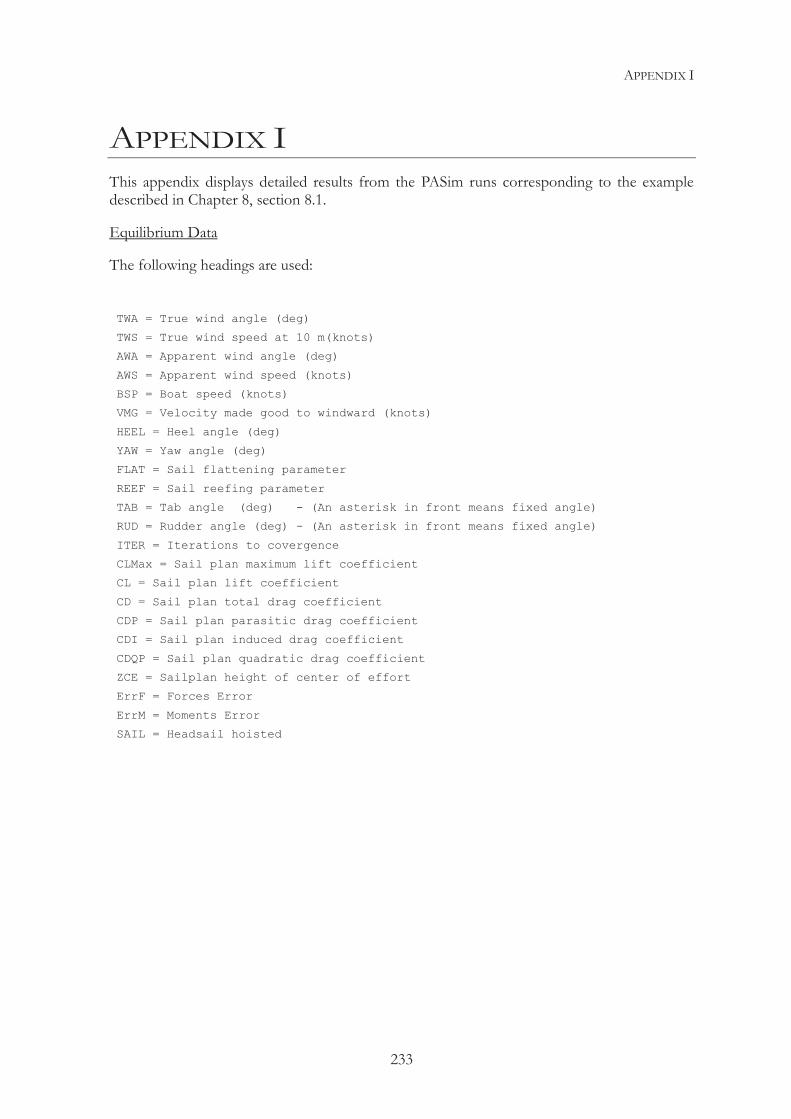
APPENDIX I
233
APPENDIX I This appendix displays detailed results from the PASim runs corresponding to the example described in Chapter 8, section 8.1.
Equilibrium Data
The following headings are used:
TWA = True wind angle (deg)
TWS = True wind speed at 10 m(knots)
AWA = Apparent wind angle (deg)
AWS = Apparent wind speed (knots)
BSP = Boat speed (knots)
VMG = Velocity made good to windward (knots)
HEEL = Heel angle (deg)
YAW = Yaw angle (deg)
FLAT = Sail flattening parameter
REEF = Sail reefing parameter
TAB = Tab angle (deg) - (An asterisk in front means fixed angle)
RUD = Rudder angle (deg) - (An asterisk in front means fixed angle)
ITER = Iterations to covergence
CLMax = Sail plan maximum lift coefficient
CL = Sail plan lift coefficient
CD = Sail plan total drag coefficient
CDP = Sail plan parasitic drag coefficient
CDI = Sail plan induced drag coefficient
CDQP = Sail plan quadratic drag coefficient
ZCE = Sailplan height of center of effort
ErrF = Forces Error
ErrM = Moments Error
SAIL = Headsail hoisted
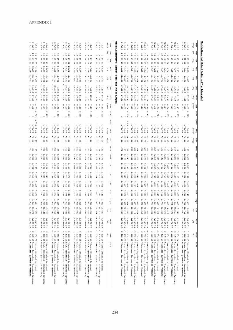
APPENDIX I
234
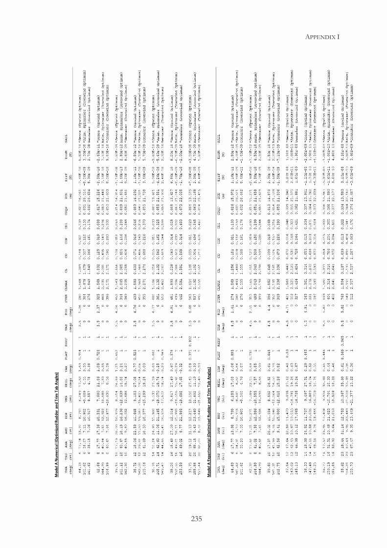
APPENDIX I
235
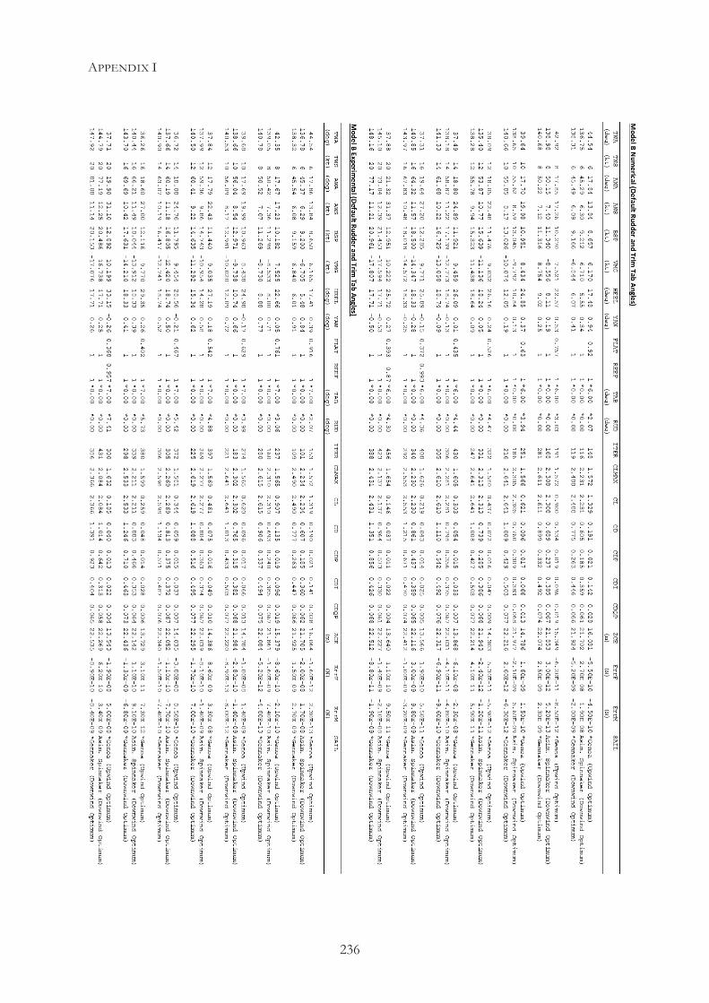
APPENDIX I
236
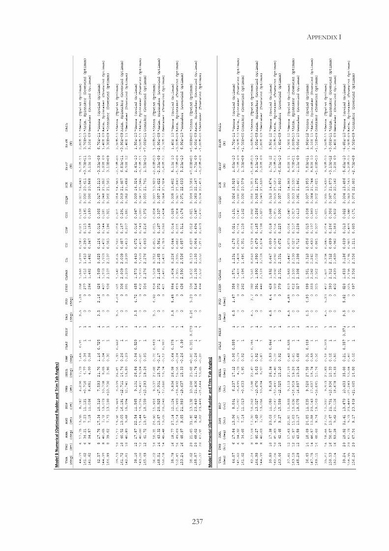
APPENDIX I
237
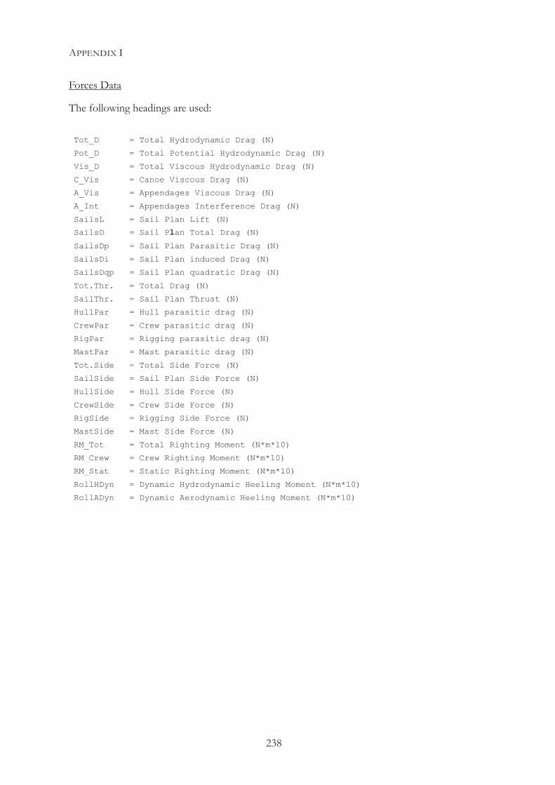
APPENDIX I
238
Forces Data
The following headings are used: Tot_D = Total Hydrodynamic Drag (N)
Pot_D = Total Potential Hydrodynamic Drag (N)
Vis_D = Total Viscous Hydrodynamic Drag (N)
C_Vis = Canoe Viscous Drag (N)
A_Vis = Appendages Viscous Drag (N)
A_Int = Appendages Interference Drag (N)
SailsL = Sail Plan Lift (N)
SailsD = Sail Plan Total Drag (N) SailsDp = Sail Plan Parasitic Drag (N)
SailsDi = Sail Plan induced Drag (N)
SailsDqp = Sail Plan quadratic Drag (N)
Tot.Thr. = Total Drag (N)
SailThr. = Sail Plan Thrust (N)
HullPar = Hull parasitic drag (N)
CrewPar = Crew parasitic drag (N)
RigPar = Rigging parasitic drag (N)
MastPar = Mast parasitic drag (N)
Tot.Side = Total Side Force (N)
SailSide = Sail Plan Side Force (N)
HullSide = Hull Side Force (N)
CrewSide = Crew Side Force (N)
RigSide = Rigging Side Force (N)
MastSide = Mast Side Force (N)
RM_Tot = Total Righting Moment (N*m*10)
RM_Crew = Crew Righting Moment (N*m*10)
RM_Stat = Static Righting Moment (N*m*10)
RollHDyn = Dynamic Hydrodynamic Heeling Moment (N*m*10)
RollADyn = Dynamic Aerodynamic Heeling Moment (N*m*10)
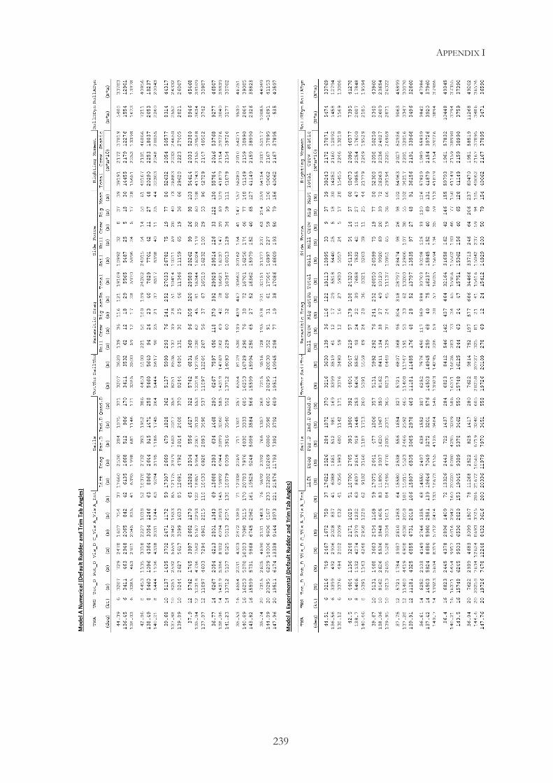
APPENDIX I
239
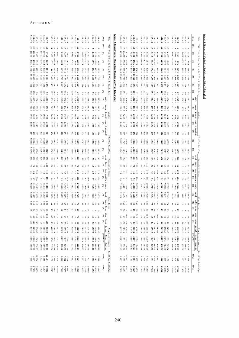
APPENDIX I
240
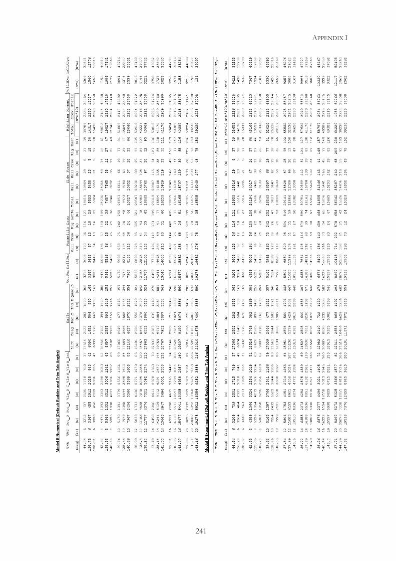
APPENDIX I
241
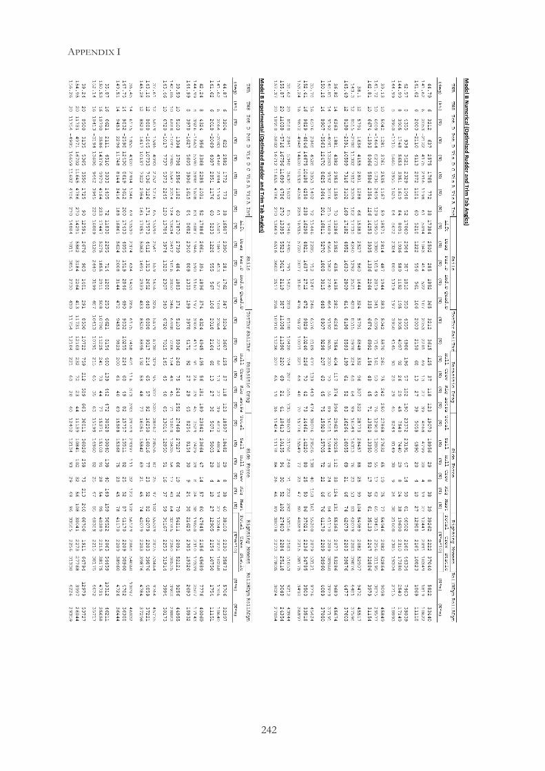
APPENDIX I
242
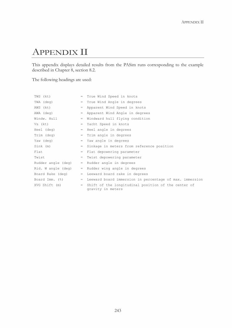
APPENDIX II
243
APPENDIX II This appendix displays detailed results from the PASim runs corresponding to the example described in Chapter 8, section 8.2.
The following headings are used:
TWS (kt) = True Wind Speed in knots
TWA (deg) = True Wind Angle in degrees
AWS (kt) = Apparent Wind Speed in knots
AWA (deg) = Apparent Wind Angle in degrees
Windw. Hull = Windward hull flying condition
Vs (kt) = Yacht Speed in knots
Heel (deg) = Heel angle in degrees
Trim (deg) = Trim angle in degrees
Yaw (deg) = Yaw angle in degrees
Sink (m) = Sinkage in meters from reference position
Flat = Flat depowering parameter
Twist = Twist depowering parameter
Rudder angle (deg) = Rudder angle in degrees
Rid. W angle (deg) = Rudder wing angle in degrees
Board Rake (deg) = Leeward board rake in degrees
Board Imm. (%) = Leeward board immersion in percentage of max. immersion
XVG Shift (m) = Shift of the longitudinal position of the center of gravity in meters
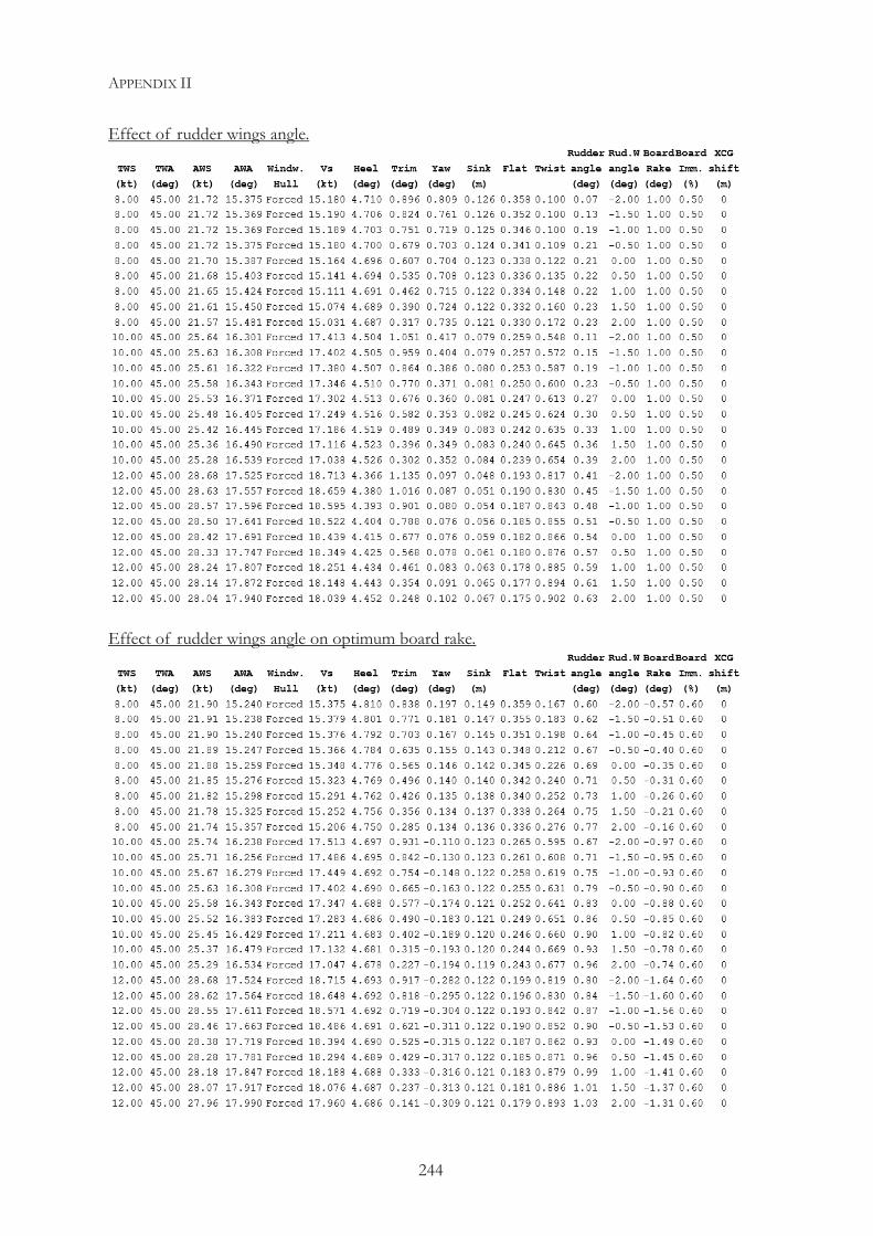
APPENDIX II
244
Effect of rudder wings angle.
Effect of rudder wings angle on optimum board rake.
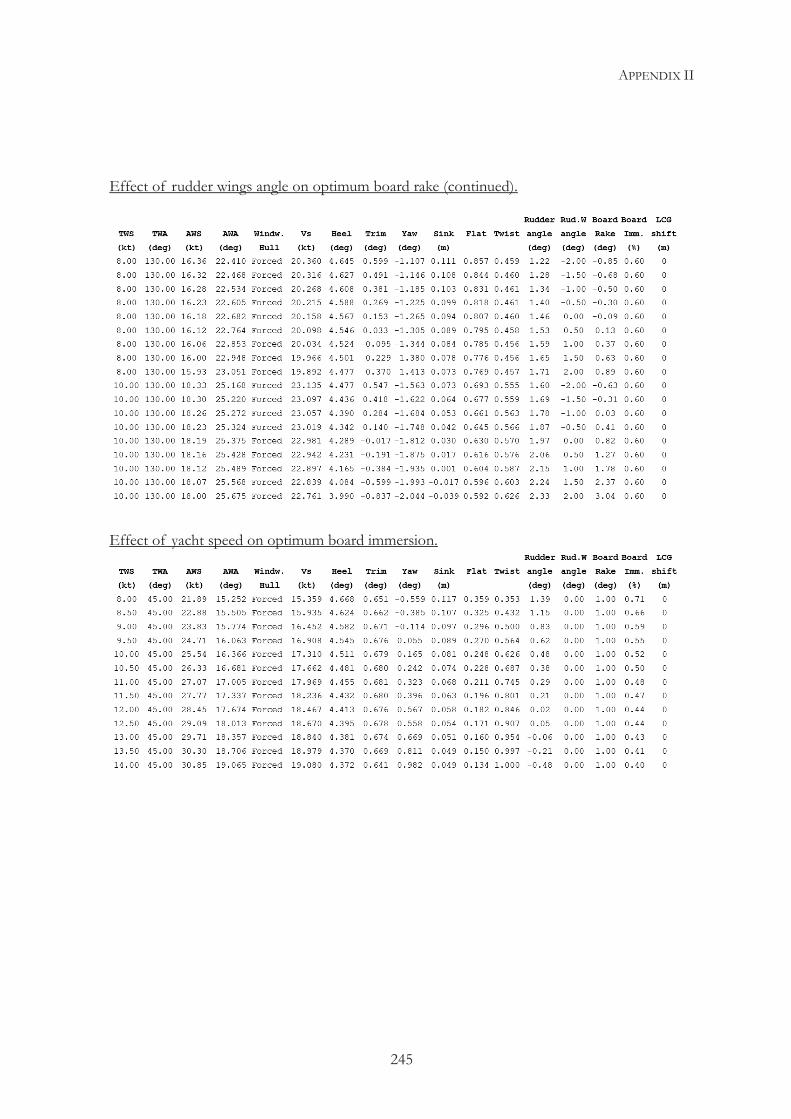
APPENDIX II
245
Effect of rudder wings angle on optimum board rake (continued).
Effect of yacht speed on optimum board immersion.
p p
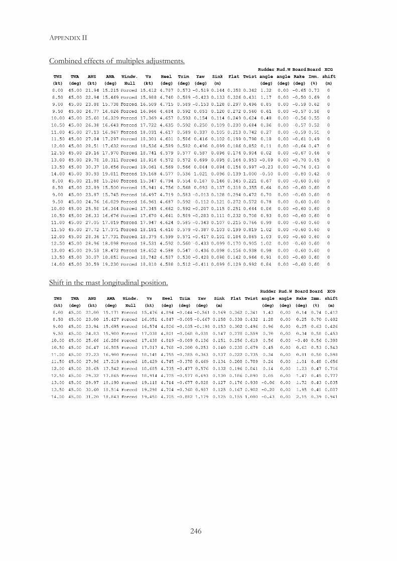
APPENDIX II
246
Combined effects of multiples adjustments.
Shift in the mast longitudinal position.
j


![Grandes Batallas Navales - [03de12] Jutlandia [Spanish E-book][by Alphacen]](https://img.pdfslide.us/doc/110x75/577cd67e1a28ab9e789c8601/grandes-batallas-navales-03de12-jutlandia-spanish-e-bookby-alphacen.jpg)

![Grandes Batallas Navales - [12de12] Okinawa (y2) [Spanish E-book][by Alphacen]](https://img.pdfslide.us/doc/110x75/577cd67a1a28ab9e789c7a65/grandes-batallas-navales-12de12-okinawa-y2-spanish-e-bookby-alphacen.jpg)

![Grandes Batallas Navales - [11de12] Okinawa [Spanish E-book][by Alphacen]](https://img.pdfslide.us/doc/110x75/577cd67a1a28ab9e789c7a55/grandes-batallas-navales-11de12-okinawa-spanish-e-bookby-alphacen.jpg)