Embed Size (px)
Citation preview

DENTAL IMPLANT STABILITY ANALYSIS BY USING
RESONANCE FREQUENCY METHOD
By
Reza Harirforoush
M. Sc., Islamic Azad University, Tehran South Branch 2003
B. Sc., Islamic Azad University, Tehran Central Branch 2001
THESIS SUBMITTED IN PARTIAL FULFILLMENT OF
THE REQUIREMENTS FOR THE DEGREE OF
MASTER OF APPLIED SCIENCE
In the
School of Engineering Science
Faculty of Applied Sciences
© Reza Harirforoush 2012
SIMON FRASER UNIVERSITY
Summer 2012
All rights reserved. However, in accordance with the Copyright Act of Canada, this work may be
reproduced, without authorization, under the conditions for Fair Dealing. Therefore, limited reproduction of
this work for the purposes of private study, research, criticism, review and news reporting is likely to be in
accordance with the law, particularly if cited appropriately.

ii
APPROVAL
Name: Reza Harirforoush
Degree: Master of Applied Science
Title of Thesis: Dental Implant Stability Analysis by using Resonance
Frequency Method
Examining Committee:
Chair: Dr. M. Moallem
Associate Professor of Engineering Science
___________________________________________
Dr. Siamak Arzanpour
Senior Supervisor
Assistant Professor of Engineering Science
___________________________________________
Dr. G.Wang
Supervisor
Professor of Engineering Science
___________________________________________
Dr. Woo Soo Kim
Internal Examiner
Assistant Professor of Engineering Science
Date Defended/Approved: July 26, 2012

iii
Partial Copyright Licence

iv
ABSTRACT
The use of dental implants in the rehabilitation of partially and completely edentulous
patients has been significantly increased in recent years. Although high survival rates of
implants supporting prosthesis have been reported, failure still happens due to bone loss
as results of primary and secondary implant stability. Primary stability of an implant
mostly comes from mechanical interaction with cortical bone while secondary stability
happens through bone regeneration and remodelling at the implant/bone interface.
Defining the implant stability remains a challenge in dentistry and several researches
have been made in this field. To detect implant stability, various diagnosis analyses have
been employed. Among them, resonance frequency analysis (RFA) is an objective
method of monitoring implant/tissue integration.
In this thesis, experimental and numerical studies are carried out to find the effect of
some parameters affecting the stability of dental implant by using RFA. Modal analysis
technique is employed to investigate the effect of coupled mode shapes in dental implant.
Moreover, the primary stability of dental implant that indicates the process of bone-
implant integration is investigated. Resonance frequency of jaw-implant structure is
carried out using finite element modelling. Different implant-bone interface conditions
are studied for this investigation. The effects of endosseous implant angulation on the
resonance frequency of implant are studied. MIMICS, a three dimensional (3D)
modelling software was used to construct a 3D model of a pig mandible from computed
tomography (CT) images. The resonance frequency of the implant was analyzed using
finite element (FE) modal analysis in a simulated environment. The MIMICS is also used
to investigate effect of soft tissue surrounding the implant on the RF of implant. In
addition, three different pig mandibles were employed to assess the effect of some
parameters affecting resonance frequency of implant. Finally, experimental studies are
carried out to investigate the effect of soft tissue on RF of implant. A novel device is also
designed for stability analysis of dental implants.
Keywords: Implant stability, resonance frequency, modal analysis, finite element
method, MIMICS

v
ACKNOWLEDGEMENTS
In the name of Allah, the Most Gracious and the Most Merciful
It would not have been possible to write this M.Sc. thesis without the help and
support of the kind people around me, to only some of whom it is possible to give
particular mention here. This thesis would not have been possible without the help,
support and advice of my supervisor, Prof. S. Arzanpour. I have been extremely lucky to
have a supervisor who cared so much about my work, and who responded to my
questions and queries so promptly. His positive and friendship personality has continually
inspired me. The good advice and support of my UBC supervisor, Dr. B. Chehroudi, has
been invaluable on both an academic and a personal level, for which I am extremely
grateful. I also thank the Department of MSE for their support and assistance especially
the head of department, Prof. F. Golnaraghi. The library facilities and computer facilities
of the SFU have been indispensable. I would like to thank Prof. Carolyn Sparrey for her
kindness; friendship and support to allow me using MIMICS software. I would also like
to thank my colleagues and friends in the Dental Engineering Lab, E. Asadi, Ciara and V.
Zakeri, H. Dehghani.
Above all, I deeply would like to thank my lovely wife, Mahsa, for her personal
support and great patience at all times. My parents, brother, brothers in law, sister and
sisters in law have given me their unequivocal support throughout, as always, for which
my mere expression of thanks likewise does not suffice.

vi
TABLE OF CONTENTS
Approval .............................................................................................................................................................ii
Partial Copyright Licence ....................................................................................................................... iii
Abstract .............................................................................................................................................................iv
Acknowledgements ........................................................................................................................................ v
Table of Contents ..........................................................................................................................................vi
List of Figures ............................................................................................................................................. viii
List of Tables ................................................................................................................................................... xi
Nomenclature ................................................................................................................................................ xii
1: Introduction ...................................................................................................................................................1
1.1 Available methods currently used to assess implant stability ........................................................... 2
1.1.1 Radiographic analysis .................................................................................................................... 2 1.1.2 Cutting Torque Resistance Analysis (CRA) ........................................................................... 3 1.1.3 Reverse Torque Test (RTT) ......................................................................................................... 3 1.1.4 Insertion torque analysis ................................................................................................................ 4 1.1.5 Percussion test .................................................................................................................................. 4 1.1.6 Pulsed oscillation waveform ........................................................................................................ 5 1.1.7 Impact hammer method ................................................................................................................. 5 1.1.8 Resonance Frequency Analysis (RFA) ..................................................................................... 7 1.1.9 Finite Element Analysis (FEA) ................................................................................................... 9 1.1.10 Ultrasonic wave propagation .................................................................................................... 10
1.2 Contribution ................................................................................................................................................... 10
2: The effect of coupled mode shapes in dental implant ................................................................... 14
2.1 Introduction to modal analysis ................................................................................................................. 14
2.2 Theoretical basis ........................................................................................................................................... 15
2.2.1 SDOF system theory .................................................................................................................... 15 2.2.2 MDOF systems with viscous damping .................................................................................. 16 2.2.3 The theory of analysis of coupled structures........................................................................ 17
2.3 Experimental setup ....................................................................................................................................... 18
2.4 FEM modelling of dental implant and coupled structure (implant/chuck) ................................ 20
2.5 Results and discussion ................................................................................................................................ 22
2.6 Conclusion ...................................................................................................................................................... 22
3: A numerical approach of estimating dental implant healing process using
Resonnace Frequency Analysis (RFA) .................................................................................................... 26
3.1 Materials and Methods................................................................................................................................ 26
3.2 Results .............................................................................................................................................................. 29
3.3 Conclusion ...................................................................................................................................................... 34

vii
4: The effect of endosseous implant angulation on the resonance frequency of
implant ............................................................................................................................................................... 35
4.1 Material and methods .................................................................................................................................. 36
4.1.1 Pig mandible model ..................................................................................................................... 36 4.1.2 Simplified Epoxy cubical model A & B................................................................................ 40
4.2 Results .............................................................................................................................................................. 42
4.2.1 Pig mandible model ..................................................................................................................... 42 4.2.2 Simplified Epoxy cubical model A & B................................................................................ 43
4.3 DISCUSSION ..................................................................................................................................................... 47
4.4 CONCLUSION ................................................................................................................................................... 50
5: The effect of soft tissue surrounding the implant on the resonance frequency of
implant ............................................................................................................................................................... 51
5.1 Materials and methods ................................................................................................................................ 52
5.1.1 The modelling of the pig jaw and soft tissue ........................................................................ 52 5.1.2 Parametric studies ......................................................................................................................... 54 5.1.2.1 The effect of the size .................................................................................................................... 54 5.1.2.2 The effect of location ................................................................................................................... 55
5.2 Results .............................................................................................................................................................. 58
5.3 Discussion ....................................................................................................................................................... 67
5.4 Conclusion ...................................................................................................................................................... 68
6: Experiments on pig jaw ......................................................................................................................... 69
6.1 The effect of free length on resonance frequency of implant ......................................................... 70
6.1.1 Accelerometer results .................................................................................................................. 70 6.1.2 Microphone results ....................................................................................................................... 72
6.2 The effect of implant size on resonance frequency of implant ...................................................... 72
6.3 Comparison between the RF of implant inserted in a segment and whole pig
mandible .......................................................................................................................................................... 73
7: Experimental studies to find the effect of surrounding soft tissue on RF of implant ......... 75
7.1 Material and Methods ................................................................................................................................. 75
7.2 Results .............................................................................................................................................................. 78
7.3 Conclusion ...................................................................................................................................................... 80
8: Conclusions and Recommendations.................................................................................................... 82
9: Reference List ............................................................................................................................................. 84

viii
LIST OF FIGURES
Figure 1-1: The picture of lower jaw and teeth ................................................................................ 5
Figure 1-2: Periotest device .............................................................................................................. 6
Figure 1-3: Osstell Device ................................................................................................................ 9
Figure 2-1: schematic of hardware used in performing a vibration test ......................................... 15
Figure 2-2: Single degree of freedom (SDOF) system .................................................................. 15
Figure 2-3: Basis of FRF coupling analysis ................................................................................... 18
Figure 2-4: Test setup of implant modal analysis........................................................................... 19
Figure 2-5: Test setup of implant/chuck modal analysis ................................................................ 20
Figure 2-6: Model of implant meshed in ANSYS .......................................................................... 21
Figure 2-7: 3D model of implant/chuck meshed in ANSYS .......................................................... 22
Figure 2-8- Experimental results of RF of implant for different free length ................................. 23
Figure 2-9: Plot of RF versus different free length of dental implant ............................................ 24
Figure 2-10: The modes of implant/chuck system correspond to free length 9.44 mm and
8.88 mm ....................................................................................................................... 25
Figure 3-1 (A): The assembled model ............................................................................................ 29
Figure 3-1 (B): Cross section of implant, cortical and Cancellous rings........................................ 29
Figure 3-1 (C): The components of implant-bone structure model ................................................ 29
Figure 3-2: The resonance frequencies under different cortical and cancellous bone levels
in combination 1 when 8 mm of implant is left out of bone ........................................ 31
Figure 3-3: The resonance frequencies under different cortical and cancellous bone
levels in combination 2 when 8 mm of implant is left out of bone .............................. 31
Figure 3-4: The resonance frequencies under different cortical and cancellous bone levels
in combination 1 when 8 and 7 mm of implant is left out of bone .............................. 32
Figure 3-5: The resonance frequencies under different cortical and cancellous bone levels
in combination 2 when 8 and 7 mm of implant is left out of bone .............................. 32
Figure 3-6 : The mode shapes of implant for 10% surrounding bone Young’s modulus in
case of 8mm of implant left out of the bone for combination ...................................... 33
Figure 4-1: (a) a section of pig mandible. (b) Transveres plane of one of CT image slices
of sectioned pig mandible (c) A CT image slice in which the cortical,
cancellous bone, enamel and dentine are shown (d) 3D model of pig
mandible showing bone, teeth, implant and abutment ................................................. 39
Figure 4-2: The centre of mass of implant is rotated about y-axis from 1º to 10º in 1º
increments. ................................................................................................................... 40
Figure 4-3: simplified bone models (model A & B) ...................................................................... 41
Figure 4-4: The parameter h defined as the distance between reference point and
reference coordinate system ......................................................................................... 42

ix
Figure 4-5: The RF and CCBR values with respect to angles in model B .................................... 45
Figure 4-6: The RF and CCBR values with respect to angles in pig mandible model .................. 46
Figure 4-7: The behaviour of RF of implant versus CCBR for different implant
orientations ................................................................................................................... 47
Figure 4-8: The mode shapes of implant for the case of implant is buried in the bone and
it is rotates 1 degree around y-axis ............................................................................... 50
Figure 5-1: A slice of CT image that showing the soft tissue built as 4/8 hollow
cylindrical section in interfacing areas of implant and bone ........................................ 53
Figure 5-2: Transverse and coronal views of a slice of CT image showing the soft tissue
as 4/8 and 6/8 hollow cylindrical section suroudnig the implant, and the 3D
models of both implant and soft tissues ....................................................................... 56
Figure 5-3: 3D modesl of two different heigths of soft tissue when it is built as 4/8 hollow
cylindrical section. ....................................................................................................... 57
Figure 5-4: 3D soft tissue is constructed as 2/8 hollow cylindrical section and is moved
along z axis ................................................................................................................... 57
Figure 5-5: 3D soft tissue constructed as 1/8 hollow cylindrical section and rotates around
z axis ............................................................................................................................ 58
Figure 5-6: The results of the resonance frequencies corresponding to the soft tissue when ......... 59
Figure 5-7: The results of the resonance frequencies of implant when the soft tissue is
built as 2/8 hollow cylindrical section around the implant and the height of it
increases from 2 mm to 10 mm in 1 mm steps ............................................................. 60
Figure 5-8: The results of the resonance frequencies of implant when the soft tissue is
built as 4/8 hollow cylindrical section around the implant and the heigth of it
increases from 2 mm to 10 mm in 1 mm steps ............................................................. 61
Figure 5-9: The results of the resonance frequencies of implant when the soft tissue is
built as 6/8 hollow cylindrical section around the implant and the heigth of it
increases from 2 mm to 10 mm in 1 mm steps ............................................................. 61
Figure 5-10: The results of the resonance frequencies of implant when the soft tissue is
built as 8/8 hollow cylindrical section around the implant and the height of it
increases from 2 mm to 10 mm in 1 mm steps ............................................................. 62
Figure 5-11: The results of the resonance frequencies of implant when the soft tissue is
built as 2/8, 4/8, 6/8 and 8/8 hollow cylindrical section around the implant and
the height of it increases from 2 mm to 10 mm in 1 mm steps .................................... 62
Figure 5-12: The resonance frequencies of the soft tissue when it is built as 2/8 hollow
cylindrical section and moves along z axis, : KHz....................................................... 64
Figure 5-13: The resonance frequencies of the soft tissue when it is built as 1/8 hallow
circle and rotates around the center of implant, shown in Figure 5-6: KHz ................ 66
Figure 5-14: The results of resonance frequencies of the soft tissue built as 2/8 circle and
the height of it increases from 2 mm to 10 mm ........................................................... 67
Figure 6-1: In vivo test set up ......................................................................................................... 70
Figure 6-2: The FFT of different free length of implant in pig No.1 ............................................. 71

x
Figure 6-3: The FFT of different free length of implant in pig No.3 ............................................. 72
Figure 6-4: Comparison between the RF of implant in selected and whole pig mandible ............. 74
Figure 7-1: Test set up .................................................................................................................... 78
Figure 7-2: (a) FRF of microphone when the soft tissue is removed and the implant is
contacted with metal chuck (b) FRF of microphone when the soft tissue is
adhered to the implant and the chuck is rotated 1000 around its centre ........................ 79
Figure 7-3: The RFs of implant when the chuck is rotated from 00 to 360
0 around its
centre in 100 increments ............................................................................................... 80
Figure 7-4: The mean values of RFs of implant when the chuck is rotated from 00 to 360
0
around its centre in 100 increments .............................................................................. 80

xi
LIST OF TABLES
Table 2-1: Material property of the implant ................................................................................... 21
Table 2-2: RF of dental implant under different chuck levels ........................................................ 23
Table 3-1: Different combinations of the bone’s material properties ........................................... 33
Table 4-1: Material properties of the 3D segment of pig mandible .............................................. 38
Table 4-2: Results of model A & B ................................................................................................ 44
Table 4-3: Results of pig mandible ................................................................................................ 46
Table 5-1: Material properties of the partial pig jaw model ........................................................... 54
Table 5-2: The resonance frequencies corresponding to the soft tissue when it is built as
an apporximately 1/8 hollow cylindrical section and increases from 1/8 to 8/8:
KHz .............................................................................................................................. 58
Table 5-3: The resonanace frequencies corresponding to the soft tissue built as 2/8, 4/8,
6/8 and 8/8 hollow cylindrical section and the heigth of each case increases
from 2 mm to 10 mm in 1 mm steps: KHz ................................................................... 60
Table 5-4: The absolute differences of resonance frequencies corresponding to the soft
tissue when it is built as 2/8, 4/8, 6/8 and 8/8 circle and the heigth increases
from 2 mm to 10 mm : Hz ............................................................................................ 63
Table 5-5: The resonance frequencies corresponding tothe soft tissue when it is built as
2/8 hollow cylindrical section and moves along z axis, Fig. 7: KHz ........................... 64
Table 5-6: The perpendicular resonance frequencies corresponding tothe soft tissue when
it is built as 1/8 circle and rotates around the center of implant: KHz ......................... 65
Table 5-7: The resonance frequencies of implant in case the soft tissue is constructed as
2/8 circle and the heigth of it increases from 2 mm to 10 mm:KHz ............................ 66
Table 6-1: The FFT of different free length of implant in pig No.2 ............................................... 72

xii
NOMENCLATURE
m Mass
c Damper
k Stiffness
Frequency response function
[M] Mass matrix
[C] Damping matrix
[K] Stiffness matrix
P Normalized eigenvectors
l Length
I moment of inertia
E Modulus f elasticity
density
Absolute difference
Greek symbols
Natural frequency
Undamped natural frequency
ξ critical damping ratio
receptance matrix
Resonance frequency
Constant
Poisson`s ratio
Damped natural frequency
Subscript
CRA Cutting Torque resistant Analysis
RTT Reverse Torque Test
RTV Reverse Torque Value
POWF Pulse Oscillation Wave Form
FFT Fast Fourier Transform
DMC Dental Mobility Checker
CT Contact Time / Computed Tomography
RFA Resonance Frequency Analysis
DOF Degree of Freedom
RF Resonance Frequency
ISQ Implant Stability Quotient
FEA Finite Element Analysis
FE Finite Element

xiii
FEM Finite Element Method
QUS Quantitative Ultrasound
CCBR Cortical to Cancellous Bone Ratio
SDOF Single Degree of Freedom
MDOF Multi Degree of Freedom
FRF Frequency Response Function
CBCT Cone Beam Computed Tomography
RP Reference Point
RCS Reference Coordinate System

1
1: INTRODUCTION
The use of dental implants in the rehabilitation of partially and completely
edentulous patients has been significantly increased in dentistry since 1980 [1].
Although high survival rates of implants supporting prosthesis have been reported
[2,3,4], failure still happens due to bone loss as a results of primary and secondary
implant stability. Primary stability of an implant is the absence of mobility in the bone
bed upon insertion of the implant and mostly comes from mechanical interaction with
cortical bone. It is also named as “Mechanical Stability” which is the result of
compressed bone holding the implant tightly in the bone. Secondary stability, named
as “Biological Stability”, happens through bone regeneration and remodelling at the
implant/bone interface [5,6]. It is the result of new bone cells forming at the site of the
implant and osseointegration. The primary stability is the requirement for successful
secondary stability [6]. Secondary stability orders the time of functional loading [7].
Following the placement of an endosseous implant, primary mechanical stability
gradually decreases and secondary stability (biologic) gradually increases.
Bone quantity and quality, surgical techniques including the skill of the surgeon,
implant (geometry, length, diameter, and surface characteristics) are major factors
affecting primary stability [8]. Primary stability, bone modelling and remodelling, and
implant surface conditions are the main parameters influencing secondary stability [8].
Osseointegration is an important factor in specifying a series of criteria that
identifies success or failure of an implant. Osseointegration is, however, a patient-
dependent wound healing process that happens at two different stages: primary
stability and secondary stability.
Dental implant stability measurement, an indirect indication of osseointegration,
is a measurement of implant’s resistance to movement [9]. Objective measurement of
implant stability is a valuable tool for achieving consistently good results first and
foremost because implant stability plays such an important role in achieving a

2
successful outcome. The advantages of measuring implant stability are to make more
accurate decisions about the time of crown loading or unloading, select the protocol of
choice for implant loading, and increase trust between patient and practitioner. It is,
therefore important to be able to quantify implant stability at various times and have in
place a long-term prognosis based on implant stability measurement tool. Although
various diagnosis analyses have been employed and several research and development
projects have been already made in this field, measuring implant stability remains a
challenge in dentistry.
1.1 Available methods currently used to assess implant stability
In this section, the currently available methods to evaluate implant stability are
discussed. The methods for studying stability can be categorized as invasive, which interfere
with the osseointegration process of the implant, and non-invasive, which do not. Some of
the most famous methods in analyzing dental implant stability are histologic analysis,
percussion test, radiographs, reverse torque, cutting resistance, and resonance frequency
analysis (RFA). Since histologic analysis is not feasible for daily practice it is not
discussed in this chapter.
1.1.1 Radiographic analysis
Radiographic analysis was one of the first methods applied to evaluate the
condition of implants after they had been placed. Radiographic evaluation is a non-
invasive method that can be performed at any stage of healing process. Bitewing
radiographs are used to measure crestal bone level, defined as the distance from the top of
the implant to the position of the bone on the implant surface, because it has been
suggested as an indicator for implant success [10]. However, other studies recommended
that the resolution of bitewing radiographs cannot be used as the only tool to evaluate
either primary or secondary stability [8]. Moreover, crestal bone changes can be only
reliably measured if there is no distortion in the radiographic pictures. In those pictures,
the distortion happens when the central x-ray tube is not positioned parallel to the
implant. Furthermore, panoramic view (a dental X-ray scanning of the upper and lower

3
jaw that shows a two-dimensional view of a half circle from ear to ear) does not provide
information on a facial bone level, and bone loss. Finally, regular radiographs cannot be
used to quantify neither bone quality nor density. They can be used to assess changes in
bone mineral only when there are decreases that exceed 40% of the initial mineralization
[11]. Moreover, because of X-radiation hazards other methods with fewer side effects are
preferred.
1.1.2 Cutting Torque Resistance Analysis (CRA)
This method was originally developed in 1994 by Johansson and Strid [12] and
later improved in vitro and in vivo human models. In this method the energy (
)
required in cutting off a unit volume of bone during implant surgery is measured. This
energy has been shown to be significantly correlated with bone density, which has
been suggested as one factor that significantly influences implant stability [13]. The
advantages of this method are detecting bone density and its quality during surgery.
The major limitation of CRA is that it does not give any information on bone quality
until the osteotomy site (a surgical operation for bone shortening or realignment) is
prepared. In addition, this information cannot be used to assess bone quality changes
after implant insertion.
1.1.3 Reverse Torque Test (RTT)
The Reverse Torque Test (RTT), which is proposed in 1984 by Roberts et al.
[14], measures the critical torque threshold when bone-implant contact is broken. This
indirectly provides information on the degree of bone-implant contact in a given
implant. Removal Torque Value (RTV) as an indirect measurement of bone-implant
contact was reported to range from 45 to 48 N.cm [15]. The disadvantage of this
method is the risk of irreparable plastic deformation within implant bone integration
and the implant failure when unnecessary load is applied to an implant that is still
undergoing osseointegration. In addition, applying torque on implants placed in bone
of low quality may result in a shearing of bone-to-implant contact and cause implants
to irretrievably fail.

4
1.1.4 Insertion torque analysis
Insertion torque analysis, as an invasive method, expresses the amount of force
that is applied to the implant as it is inserted. Implant placement insertion torque is
initially minimal, and increases quickly until the cortical layer (see Figure 1-1) in a
jawbone is fully engaged. As the implant is driven into the bone, repeated measurements
are taken and a graph is often produced. The maximum value is obtained when the head
of the screw makes contact with the cortical plate (the hard, outer shell of alveolar).
Insertion torque measurement includes finding the maximum insertion torque value when
the screw head contacts the cortical plate. This test has been generally well accepted and
has been used for evaluating various implant designs [16]. Insertion torque has been
found to correlate with bone density and consequently implant stability [17]. The
application of insertion torque has been shown to be limited since estimating the quality
of the bone is impossible until the implant insertion is actually started. So, insertion
torque measurements cannot be used for the selection of implant sites. This method also
cannot be used to follow implant healing and osseointegration procedures.
Figure 1-1 : The picture of lower jaw and teeth
1.1.5 Percussion test
Percussion test is the simplest method for testing implant stability. This test is
based upon vibrational acoustic science and impact-response theory. In this method,

5
clinical judgment about osseointegration is made based on the sound heard from the
percussion of the implant with a metallic instrument. A “crystal” sound indicates
successful osseointegration, while a “dull” sound means weak or failing osseointegration.
This method heavily relies on the clinician’s experience level and subjective belief.
Therefore, it cannot be used experimentally as a standard testing method.
1.1.6 Pulsed oscillation waveform
Kaneko et al. [18,19] used a Pulsed Oscillation Wave Form (POWF) to analyze
the mechanical vibrational characteristics of the implant-bone interface using forced
excitation of a steady-state wave.
Pulsed oscillation waveform works based on the frequency and amplitude of the
implant vibration induced by a small-pulsed force. This system consists of an
acoustoelectric driver, an acoustoelectric receiver, a pulse generator and an oscilloscope.
Both the acoustoelectric driver and the acoustoelectric receiver consist of a piezoelectric
element and a puncture needle. A multifrequency pulsed force of about 1 KHz is applied
to the implant by lightly touching it with two fine needles connected to piezoelectric
elements. Resonance and vibration generated from the bone-implant interface of an
excited implant are picked up and displayed on an oscilloscope. The sensitivity of this
method depended on load directions and positions. The sensitivity of this method is low
for the assessment of implant rigidity [18].
1.1.7 Impact hammer method
Impact hammer is an example of transient force as a source of excitement. This
method is an improved version of the percussion test except that sound generated from
contact between hammer and object is processed through fast Fourier transform (FFT).
Dental Mobility Checker (DMC; J.Morita, Suita, Japan) and Periotest (Siemens,
Bensheim, Germany) are currently available devices working based on impact hammer
method.
The DMC was originally developed by Aoki and Hirakawa [20,21]. It detected
the level of tooth mobility by converting the integration of teeth and alveolar bone into

6
acoustic signals. Contac time between the tapping impact hammer and the object is
measured. In this theory, the width of the first peak on the time axis of the spectrum
generated by transient impulse is inversely proportional to the time axis of the impulse
[22]. The lower rigidity of implant-bone integration results in a longer time response. In
this device, a microphone is used as a receiver. The response signal of the microphone is
processed in the time domain. Some problems were addressed to this method such as
difficulties of double tapping and difficulty in obtaining constant excitation.
Unlike the DMC, which applies impact force with a hammer, Periotest uses an
electromagnetically driven and electrically controlled metallic tapping rod in a headpiece
(see Figure 1-2). Response to striking is then measured by a small accelerometer
incorporated into the head of the device. Similar to DMC, the contact time (CT) between
the test object and tapping rod is measured in time domain and then converted to a value
called PTV, which is related to the damping characteristics of tissue surrounding teeth or
implant. For PTV units in the range of -8 to +13, a linear formula is used:
(1)
For PTV values ranging from +13 to +50, a quadratic formula is used:
(2)
Figure 1-2: Periotest device
The lack of sensitivity is reported as one of the shortcomings of this device [23].
This is because PTV has a very wide dynamic range (PTV is -8 to +50) of possible
responses, and the PTV of an osseointegration implant falls only in a relatively narrow
zone (-5 to +5) inside the range. Moreover, values measured from Periotest can be

7
affected by excitation conditions such as position and direction. PTV also cannot be used
to identify a “borderline implant” which may or may not be considered as a successful
osseointegration. Finally, Periotest measurements are limited because they are strongly
dependent to the orientation of the excitation source and the striking point. As a result,
despite some positive claims for the Periotest, the prognostic accuracy of the Periotest for
implant stability has been criticized for a lack of resolution, poor sensitivity and
susceptibility to operator variables [24].
1.1.8 Resonance Frequency Analysis (RFA)
In resonance frequency analysis, implants are forced to oscillate and the
frequency at which they oscillate at maximum amplitude is registered as their resonance
frequency. Similar to all distributed system, an implant can have many resonance
frequencies, each called a harmonic. The resonance frequencies are dependent on the
material, length and the quality of the supporting mechanism. Since the material and
length of the implant are constants, variations of the resonance frequency highly correlate
to the quality of the support (osseointegration).
RFA, as a method of monitoring implant/tissue integration, was first introduced
for dental applications in 1996 [25]. It is a non-invasive and objective method for short
and long-term monitoring of changes in implant stability [1,26,27]. RFA has been applied
for implant stability measurement in both humans [28-30] and animals [31-33] (in vivo)
and in vitro [25,34,32]. RFA, as a technique for measuring dental implant stability, has
attracted considerable scientific interest in recent years and an increasing number of
prominent journal papers are published about it since its first introduction.
The RFA of an implant, as it was briefly mentioned in this section, can be
influenced by some factors including implant length, implant diameter, implant
geometry, implant surface characteristic and placement position, as well as bone quality,
bone quantity, damping effect of marginal mucosa, bone implant contact, effective
implant length and connection to transducer.
Currently, there are two commercially available devices used to evaluate the
resonance frequency of implants placed into the bone, Implomates (Bio Tech One) and

8
Osstell (Integration Diagnostics). Their main difference is in the way they excite
implants.
The Implomates device (Taipei, Taiwan) has been studied extensively by Huang
et al. [32,34-37]. This device utilizes an impact force to excite an implant. There is a
small electrically driven rod inside the device that produces impact force. The received
time response signal is then transferred in frequency spectrum for analysis (range 2 to 20
KHz). The first peak in the frequency spectrum (distinguishable from the noise) indicates
the primary resonance frequency of implant. Higher frequency for the primary resonance
and the sharpness of that peak indicates a more stable implant.
Osstell measures RF by attaching a metal rod to an implant with screw connection
and exciting the rod doing a frequency sweep. The rod is excited by a small magnet that
is attached to its top that can be stimulated by magnetic pulses from a handled electronic
device (see Figure 1-3). The rod can vibrate in two directions (perpendicular to each
other) and thus it has two fundamental resonance frequencies. Implant Stability Quotient
(ISQ) is a scale developed by Osstell for implant stability. It converts the resonance
frequency values ranging from 3,500 to 8,500 Hz into an ISQ of 0 to 100. A high value
indicates greater stability, while a low value indicates instability. Values greater than 65
are recommended as successful implant stability. Even though Osstell is clinically used
but there are not much convincing data on the relation between bone-implant interface
and ISQ values [8].

9
Figure 1-3: Osstell Device
Although for clinical applications, Osstell has a better performance than the
Periotest [38], both RFA devices still have some uncertainties. Further research is needed
to establish higher reliability of these diagnostic devices.
1.1.9 Finite Element Analysis (FEA)
Finite Element Method (FEM) is a numerical technique, which facilitates the RF
analysis by providing an interface where a 3D model of an object and its support can be
developed and studied. FEM approximates the real structure with a finite number of
elements and assigns mechanical properties of objects such as Young’s Modulus, the
Poisson ratio and density. This method can simulate complex geometric shapes, material
properties, and generate various boundary conditions of the real situation, which are
difficult to produce in the laboratory. FEM simulation method has the advantage of
allowing independent control of each parameter in the Finite Element (FE) models.
The first person who used modal analysis, the study of the dynamic properties of
structures (will be explained in more details in chapter 2) together with Finite Element
Method in analysis of implant stability was Williams & Williams [39]. Since then, FEM
has gradually become an important tool in biomedical research. Wang et al. [40] used
FEM for calculating RFA to determine the identifiable stiffness range of interfacial tissue
(a thin layer surrounding the implant) of dental implants. They found that when the
Young’s modulus of the interfacial tissue is less than 15 MPa, the resonance frequencies
are significantly affected by the interfacial tissue and the influence of other parameters
10
such as geometry, boundary constraint, and material property of the bone are negligible.
One limitation of finite element modelling is that it is a numerical approach based on
many assumptions, which might not necessarily realistic to simulate real cases.
1.1.10 Ultrasonic wave propagation
An alternative method to assess implant stability is quantitative ultrasound (QUS),
as suggested initially by de Almeida et al. [41]. They used the implant as a waveguide
and showed a significant correlation between the experimental 1 MHz ultrasonic
responses of an aluminum threaded piece and the screwing depth in an aluminum block.
They concluded that Ultrasonic waves are sensitive to bone-implant interface properties.
In the same study, finite difference numerical simulations depicted an agreement between
the 1 MHz ultrasonic response of titanium wave guides and the elastic properties of
tissues surrounding the guides. Furthermore, in a recent experimental study by Mathieu et
al. [42], a 10 MHz ultrasonic device was validated with implants placed in rabbit bone.
The amount of bone surrounding prototype cylindrical titanium implants was shown to be
significantly correlated with a quantitative indicator deduced from the ultrasonic response
to a 10 MHz excitation.
1.2 Contribution
One of the objectives of this research is to investigate the effect of coupled mode
shapes in dental implant. The results of this investigation are given in chapter 2. The
effect of bone-implant osseointegration is simulated by securing the implant inside a
chuck. Modal analysis technique is used to measure the resonance frequencies of
implant-chuck coupled structure. The resonance frequencies of a dental implant fixed by
a metal chuck and excited by an impulse hammer under various fixing levels are
analyzed. Moreover, the resonance frequency of implant, as one of the components of the
implant-chuck coupled structure, is also investigated. A noncontact piezoelectric
microphone is used to acquire the vibration response of the implant. The coupled
structure was also simulated using finite element modelling in ANSYS modal analysis
simulation environment.

11
Both experimental and numerical results show that the resonance frequency of a
coupled implant/chuck is influenced by the material property of each individual units as
well as the quality of their integration. Based on the results, it is concluded that the
resonance frequencies of implant is still present but the values are changed in the coupled
structure (placed inside the chuck).
The analysis of primary stability of dental implant that indicates the process of bone-
implant integration is another objective of this research which is investigated in chapter 3.
This integration is known to happen at the boundary of the bone and dental implant
contact surface. The resonance frequency of dental implant is used as the parameter for
this investigation due to its high sensitivity to boundary condition variations. In this
chapter, RFA of the jaw-implant structure is carried out using finite element modeling.
The FEM analyses are conducted in ANSYS modal analysis simulation environment. The
FEM model of the structure includes titanium implant, cancellous and cortical bone
(cancellous (spongy) and cortical (compact) bone are two types of tissue that form
bones). Different implant-bone interface conditions are studied for this investigation.
Various boundary conditions were studied to identify natural frequencies of jaw-implant
structure. Our analysis shows that the resonance frequency of the implant increases
during the healing period and reaches a plateau when the implant-bone interface was
fully integrated. The results show that RFA can be suggested as a non-invasive, reliable
and accurate diagnostic method for assessment the healing process of dental implants.
The other subject of interest is dental implant angulation. Dental implants are ideally
placed in bone in an orientation that allows vertical transfer of occlusal forces (the force
exerted on opposing teeth when the jaws are brought into) along their long axis.
Nevertheless, optimal situations for implant placement are seldom encountered resulting
in implants placement in angulated positions, which may affect their long-term success.
The implant angulation is also influenced by several factors including surrounding
anatomical structures, occlusion, vector of occlusal forces, aesthetics, prosthetic
components, and availability of healthy hard or soft tissues. RF is one objective tool used
to monitor stability of the implant tissue integration; however, it is expected that RF
changes with alteration in implant orientation in bone and little is known about this
effect. The objective followed in chapter 4 is identifying the effects of implant angulation

12
on the resonance frequency of implant. The purpose of this study is to determine the
relation between the dental implant orientation in the bone and the RF of implant.
MIMICS, a three dimensional (3D) modelling software is used to construct a 3D model
of a pig mandible from computed tomography (CT) images. The RF of the implant is
analyzed using finite element (FE) modal analysis in a simulated environment. In
addition, a cubical model is also developed in MIMICS to investigate the parameters
concerning the relationship between RF changes and implant orientation in a simplified
environment. Implant orientation angle altered by increment of one degree until
maximum of ten degrees inclination and RF is analysed. Our analysis shows that the RF
fluctuation following altering implant orientation is strongly influenced by the contacting
cortical to cancellous bone ratio (CCBR) at the implant interface.
The effect of soft tissue surrounding the implant on the RF of implant is another
objective of this study. This has been investigated in chapter 5. The aim of this study is to
find the effect of soft tissue surrounding the implant on RF. In this study, MIMICS is
used to construct a 3D model of a pig mandible (lower jaw) from computed tomography
(CT) images. The 3D model of soft tissue is also built in interfacing areas of implant and
bone. The RF of the implant is analyzed using finite element modal analysis in a
simulated environment. A vigorous parametric study is conducted to disclose the relation
between the soft tissue surrounding the implant and the RF of implant. Our analysis
reveals that the RF of implant is mainly affected by surrounding soft tissue when the soft
tissue is formed in cortical bone. The volume of soft tissue is also a significant factor in
changing the RF of implant. This finding implies that the location and the volume of soft
tissue in interfacing areas of implant and bone are dominant parameters in changing the
RF of dental implant.
In chapter 6, three different pig mandibles are employed to assess the effect of some
parameters such as the effect of free length, and the effect of implant size on RF of
implant. In this analysis, the implants are buried in the bone and an impulse hammer
excites the implant. The vibrating signals are recorded by both an accelerometer attached
to the abutment and a microphone. Both impulse force and the vibrating signal response
are analysed to obtain the resonance frequency of implant. The results showed that the
RF of implant decreases with increasing the length of implant left out of the bone. It is

13
also showed that the size of implant inserted in jaw strongly influences the RF of implant.
The longer implant showed higher RF. No difference in RF of implant is shown when the
whole and partial pig mandible are analyzed separately.
Chapter 7 includes the experimental studies of the effect of soft tissue on RF of
implant. The implant is fixed by a rotating metal chuck stand. The effect of soft tissue is
simulated by rubber. The implant is partially covered by rubber and then placed inside
the chuck to represent the local formation of soft tissue at the implant-bone interface. The
chuck is rotated from 00 to 360
0 in 10
0 increments.
The result showed decrease of the RF of implant when the implant is surrounded by
soft tissue. The results also demonstrate that the RF is mainly affected by the angle
between the direction of the transient force and the location of the soft tissue.
In summary, the effect of coupled implant/chuck structure on RF of implant is studied.
The numerical approach is carried out to investigate the effect of soft tissue and implant
angulation on RF of implant. The effect of soft tissue is also analyzed experimentally.

14
2: THE EFFECT OF COUPLED MODE SHAPES IN
DENTAL IMPLANT
In this chapter, I will briefly provide some background about the modal analysis
technique and its governing equations. Following that, I will present the theory of modal
analysis for coupled and modified structures. Finally, the effect of coupled mode shapes
in dental implant will be investigated both experimentally and numerically.
2.1 Introduction to modal analysis
Modal analysis is the process of determining the dynamic characteristics of a
system in forms of natural frequencies, damping factors and mode shapes and using them
to formulate a mathematical model for its dynamic behaviour. Modal testing is an
experimental technique used to derive the modal model of a vibratory system.
Theoretically, this technique is based on the relation between the vibration response at
one location and excitation at the same or another location as a function of excitation
frequency.
The hardware elements required in modal analysis measurements are exciters,
transducers, and signal processing software. An exciter is a source of excitation used to
provide a known or controlled input force to a structure. A transducer is a measurement
device used to convert the mechanical motion of a structure into an electrical signal. A
processor is needed to convert the time domain signal of the transducer to frequency
domain. This arrangement is illustrated in Figure 2-1 [43].

15
Figure 2-1: schematic of hardware used in performing a vibration test
2.2 Theoretical basis
2.2.1 SDOF system theory
Although very few practical structures could be realistically modelled by a single
degree of freedom (SDOF) system, the properties of such a system are very important
because more complex multi degree of freedom (MDOF) systems can be always
represented approximately with a linear superposition of a number of SDOF systems. A
representation of a typical SDOF system is shown in Figure 2-2.
Figure 2-2: Single degree of freedom (SDOF) system
The equation of motion of the system is:
f(t) (2-1)

16
For a general forcing function f(t)=F , the candidate solution can be written as
x(t)=X , where is the frequency of excitation.
(2-2)
(2-3)
Substituting f(t), and x(t) in (2-1) we have:
(2-4)
Where is called frequency response function (FRF) [44]. A non-
dimensional version of the same expression is:
(2-5)
Where is the undamped natural frequency and ξ is the damping ratio.
(2-6)
(2-7)
2.2.2 MDOF systems with viscous damping
The general equation of motion for MDOF system with viscous damping is:
(2-8)
Where [M], [C] and [K] are mass, damping and stiffness matrixes. To study MDOF
systems, first the case where there is zero excitation in order to determine the natural
modes of the system and to this end we assume a solution to the equation of motion,
which has the form:
x(t)=u (2-9)
The receptance matrix is defined by:
(2-10)
The receptance matrix can be written as:
(2-11)
Where P is the matrix of normalized eigenvectors of the matrix
and
.

17
2.2.3 The theory of coupled structures
In some cases, a complex structure that consists of an assembly of simpler
components or substructures needs to be studied. To analyze coupled structures, the
“impedance coupling method” or the “dynamic stiffness method” can be employed. This
method is based on the frequency response properties of each individual structure and can
provide the frequency response characteristics of the coupled structure [44]. The basic
principle of coupled structure modal analysis as shown in figure 2-3 can be explained by
two components A and B connected to each other from the side. Assuming that the
dynamic of each component is considered quite independently as:
(2-12)
(2-13)
where And are defined as FRF of components A and B. Now, if the two
components are connected and make system C, applying the conditions of compatibility
and equilibrium, we have:
(2-14)
(2-15)
So that:
(2-16)
This can also be written for more DOFs as:
(2-17)
This equation shows that in coupled structures the frequency response of the
system can be extracted from the frequency response of its subsystems. In this chapter,
the effect of coupled mode shapes of bone-implant structure on resonance frequency of
implant is investigated. To simulate the effect of bone-implant integration, the implant is
placed inside a chuck. The modal analysis of coupled implant/chuck is studied by both
experimental and numerical approaches.

18
Figure 2-3: Basis of FRF coupling analysis
2.3 Experimental setup
The first step for investigating the effect of the coupled mode shapes is to do
independent analysis on the RF of each substructure. To investigate the RF of implant, a
4.2 13 mm MIS endosseous implant is suspended by a rope (see Figure 2-4) and excited
to oscillate by a transient force applied by an impulse force hammer (Dynapulse model
5800B2, Dytran instruments inc., USA). A non-contacting acoustic microphone (40BE
repolarised free field microphone, G.R.A.S sound and vibration, Denmark) is used to
record the vibration signal. Both the impulse force and the excited vibration response
signal are transferred to a personal computer. The test is repeated for five times, and the
average of five impact responses is used for each of the experiments (in total 25 tests).
The signal analyser device Photon + is used to determine the frequency response function
(FRF) of the implant. The maximum sharp value of FRF represents the resonance
frequency of implant.

19
Figure 2-4: Test setup of implant modal analysis
Following that, the RF of implant is obtained when the same implant is fixed in a
metal chuck stand under different holding intensity levels (see Figure 2-5). The implant is
excited by an impact force applied with an impulse hammer installed as an inverted
pendulum. A sliding joint is implemented in this setup in order to adjust hammer’s
position to hit the implant at the right location when the implant height is changed. The
same non-contacting acoustic microphone is used to record the vibration signal. Both the
impulse force and the induced vibration response signal are saved in the computer for
frequency analysis. The tests repeated 10 times, and the final value of each test is
obtained by averaging the 10 times triggering of the system (100 tests in total). Implant
RF is measured at different free lengths. In this study, the term “free length” is referred as
the length of implant left outside the jaw (chuck in these experiments). Twelve different
free lengths are selected and excited by impulse hammer.

20
Figure 2-5: Test setup of implant/chuck modal analysis
2.4 FEM modelling of dental implant and coupled structure
(implant/chuck)
The implant used in experimental set up is modelled in the SOLIDWORKS software
(version 2009) (see Figure 2-6). To simplify the model, the thread portion in implant is
neglected. The model is imported to ANSYS and then meshed (10,286 node / 6,159
elements) for resonance frequency analysis. Material properties of implant are considered
homogenous and isotropic. The standard material property of the titanium dental implant
is presented in Table 2-1. 3D 20-node structural solid element is used in the analysis. The
boundary condition is set to free-free analysis (approximately similar to experiment
condition of hanging the implant by a rope).

21
Figure 2-6: Model of implant meshed in ANSYS
Table 2-1: Material property of the implant
Young’s modulus E (Mpa) Poisson’s ratio Density
104.8 0.34 4430
The implant/chuck coupled structure shown in Figure 2-5 is also simulated in the
SOLIDWORKS. The model is imported to ANSYS and then meshed for resonance
frequency analysis (see Figure 2-7). The material property of implant is the same as listed
in Table 2-1. 3D 20-node structural solid element is used in this analysis since it has three
degree of freedom per node, has compatible displacement shapes and is well suited to
model curved boundaries. The nodes on the back of the chuck are set to be fixed. The
contact surfaces between implant and chuck are rigidly fixed in order to prevent the
relative motion.

22
Figure 2-7: 3D model of implant/chuck meshed in ANSYS
2.5 Results and discussion
Experimental result of resonance frequency of implant indicates that the RF of
implant suspended by soft rope happens at 73.7 KHz while analyzing the RF of implant
in ANSYS simulation environment software shows that RF occurs at 73.8 KHz.
Comparing experimental and numerical results disclose the reliably and accuracy of
simulated implant model.
Figure 2-8 shows the experimental results for three different free lengths of implant,
9.4 mm, 8.88 mm and 7.7 mm when it is fixed by the metal chuck. From Figure 2-8, it
can be seen that the peak of FRFs of the coupled system increases significantly from 11.1
KHz to 17.1 KHz. The experimental results indicate the sensitivity of RF of implant to
the free length of implant.

23
Figure 2-8: Experimental results of RF of implant for different free length
The experimental results of RF of implant when it is fixed by the metal chuck and
the free length of implant is changed are tabulated in Table 2-2. While the free length
varies from 9.4 mm to 4.29 mm, the resonance frequency changes from 11.1 KHz to 25.8
KHz. As it is shown in Figure 2-9, the correlations of resonance frequency values and the
free lengths of implant is linear in the form of y= -2.871x+38.3. This finding agrees with
the results of Haung et al. [34]. Their results showed that the natural frequency values
decreased when boundary levels were reduces. They also found that there is a linear
relation between RF of implant and the free length of implant.
Table 2-2: RF of dental implant under different chuck levels
Free Length of implant (mm)
9.3 9.4 8.88 8.59 8.06 7.7 7.58 6.48 6.27 5.61 5.41 4.29
RF(KHz) 11.1 11.1 13.1 13.5 15.4 17.1 17.3 18.2 19.8 20.7 25.1 25.8
0 0.5 1 1.5 2 2.5 3 3.5 4 4.5
x 104
50
100
150
Frequency [Hz]
FR
F [
Pa/
LB
F]
9.4 mm
8.88 mm
7.7 mm17.1 KHz
13.1 KHz
11.1 KHz

24
Figure 2-9: Plot of RF versus different free length of dental implant
Resonance frequencies of implant when it is fixed by metal chuck are also analyzed
in ANSYS modal analysis simulation environment. Figure 2-10 shows the mode shapes
of dental implant under different free lengths (9.4 mm and 8.88 mm). As it can be seen in
this figure, the RFs of implant for the free lengths of 9.4 mm and 8.88 mm are 10.79 KHz
and 13.68 KHz respectively. Comparing the analytical results and experimental results
listed in Table 2-2, validates the FEM model.
The length of implant, suspended by soft rope, is 13 mm while different free length of
implant is tested when it is fixed in metal chuck. There is an inverse relation between the
free length of implant and the RF of it (it is discussed in chapter 3). Therefore, if the
implant is shortened in order to apply same free lengths, the numerical and experimental
results of RF of implant (suspended by soft rope) will be more than 73 KHz.
Since implant-chuck structure is a coupled structure, the mode shapes shown in the
ANSYS post processing results include the mode shapes of the combination. However, to
identify the mode shapes of the implant we should only consider those results where the
implant motion is considerably higher that the chuck. In fact, that mode is the one
captured by the measurement device and appears as the natural frequency of implant in
our experimental results. Figure 2-10 shows that the RF of implant when the free length
5 6 7 8 9
12
14
16
18
20
22
24
26
Free length of implant (mm)
RF
(KH
z)

25
is 9.4 mm is the twelfth mode shape of the system while the RF of implant when the free
length is 8.88 mm is the eighteenth mode shape of system.
Free length: 9.4 mm, Frequency:10.79 KHz
Free length:8.88 mm, Frequency:13.68 KHz
Figure 2-10: The modes of implant/chuck system correspond to free length 9.44 mm and 8.88 mm
2.6 Conclusion
In conclusion, both experimental and numerical results show that the resonance
frequency of a coupled implant/chuck is influenced by the material property of each
individual units as well as the quality of their integration. Based on the results, it is
concluded that the resonance frequencies of implant is still present but the values are
changed in the coupled structure (placed inside the chuck). The RFs of implant extracted
experimentally and numerically are 73 KHz, 73.7 KHz respectively. However, when the
implant is fixed in chuck the RF of implant is dropped to 11.1 KHz (in case the free
length of implant is 9.4 mm). Since each subsystem has unique FRF, it is expected that
each coupled structure such as implant/bone should have unique RF characteristic.

26
3: A NUMERICAL APPROACH OF ESTIMATING DENTAL
IMPLANT HEALING PROCESS USING RESONANCE
FREQUENCY ANALYSIS (RFA)
Osseointegration is an important factor in specifying a series of criteria that
identifies success or failure of an implant. Several reports pointed out that the status of
healing process and early prediction can be achieved by studying the behavior of
implants in surrounding tissue [45,46].
This chapter investigates the healing process of implants by monitoring the RF of
the implant. In this study, the jaw-implant structure including titanium implant,
cancellous bone and cortical bone is modeled in ANSYS modal simulation software. As
the boundary condition of implant-bone interface changes during the healing process and
because of the sensitivity of resonance frequency to boundary condition, it is expected
that the resonance frequencies of implant changes as well. In this chapter the trend of
frequency changes is analyzed to find the effect of bone-implant integration on natural
frequency and predict the stage of healing process. For this purpose, the interface
between the implant and jawbone is modeled by two rings, each to represent the cortical
and cancellous bone. To simulate the process of integration, the mechanical properties of
these rings are changed during healing process.
3.1 Materials and Methods
Healing process in dental implants is the time duration after the surgery and
placement of implant in which the jawbone strongly bonds with implants. When dental
implant is placed in the bone, healing process becomes apparent by the new bone cells
formation at the implant site. The healing process increases continuously and it is
completed when the implant-bone interface is fully integrated. Evaluation of the healing

27
process of implant cannot be accomplished easily. Assessing the effect of boundary
condition on resonance frequency of the implant is a useful diagnosis method in early
detection of healing process. As it is stated in chapter 2, the resonance frequency of
structures, including dental implants, are related to the material properties as well as
boundary conditions. The implant-bone integration is a time variant varying boundary
condition. From the knowledge of mechanical vibration theory, resonance frequency of a
cantilever beam that is fixed at one side and free to vibrate at the end can be stated as
follows:
(3-1)
Where l is the effective vibrating length of the beam, is the vibration mass per unit until
length, I is the moment of inertia, and is a constant related to the boundary conditions
[47]. According to (3-1) changing the boundary condition can directly affect the
resonance frequency. In this study, the boundary conditions between implant and bone
contact surface is changed to simulate the healing process while l, E, I and are kept
constant.
For investigating the effect of boundary condition on RF of implant and
evaluating the healing process, a model of a jaw has been developed. In that model,
cortical and cancellous bones, which are the two main parts of osseous tissue, are
included. Two subparts, i.e. the cortical bone and cancellous bone are built similar to
model used in a paper published by Wang et al. [40]. They simulated a real bone of
bovine rib of a mature specimen. The bone-implant interfaces at the cortical and
cancellous bone are constructed as rings. Since during the healing process the boundary
condition between implant and bone changes continuously, Young’s modulus of both
cortical and cancellous rings were varied from 10% to 100 % of surrounding cortical and
cancellous Young’s modulus. To study the contribution of each of the cortical and
cancellous bone structures in the RF of the bone/implant integration, the Young’s
modulus of one of them is fixed at 10% and the other one is varied from 10% to 100%.
An implant (SEVEN system, MIS implant technologies ltd.) of 4.2 13 mm is used in
our simulations. The implant is inserted into the bone and the simulations are conducted

28
for 7 and 8 mm implant free lengths. The model is analyzed in ANSYS to obtain the RF
of dental implant (see Figure 3-1). To simplify the model and because of the negligible
effect of threads on our desired analysis the FE model did not include the thread portion.
The standard material property of implant is presented in Table 2-1. To evaluate the
effect of mechanical properties of the interface on healing process, similar to [40] two
different combinations of the bone’s material properties are considered (Table 3-1). In
addition, the cortical and cancellous bones are assumed to be homogenous and isotropic.
The coinciding nodes of the contact surfaces between cortical and cancellous bone and
rings are selected to be coincident, i.e. the displacement in all directions are all the same.
3D 20-node structural solid element is used in the analysis since it has three degree of
freedom per node, has compatible displacement shapes and is well suited to model curved
boundaries. The nodes of both lateral surfaces are fixed as boundary conditions.
Table 3-1: Differentcombinationsofthebone’smaterialproperties
Description Young`s modulus
E(Mpa)
Poisson’s ratio Density
( / 3)
Combination 1 Cortical Bone 1.158× 0.321 0.9301×
Cancellous Bone 4.115× 0.2636 3.5598×
Combination 2 Cortical Bone 3.474× 0.421 2.7902×
Cancellous Bone 12.345× 0.3636 10.6792×

29
Figure 3-1 (A): The assembled model
Figure 3-1 (B): Cross section of implant, cortical
and Cancellous rings
Figure 3-1 (C): The components of implant-bone structure model
3.2 Results
Figures 3-2 and 3-3 show the RF of the dental implant in three different case
studies for each of the combinations. The first case (shown by solid line) indicates the
situation when the Young’s modulus of both implant-bone interfaces, i.e. cortical and

30
cancellous rings, were increased from 10% to 100%. The second case (shown by dash-
dot) indicates the situation when the cancellous Young’s modulus is fixed at 10% and the
cortical Young’s modulus is increased from 10% to 100%. Finally, the third case (shown
by dash line) indicates the situation when the cortical Young’s modulus is fixed at 10%
and the cancellous Young’s modulus is changed from 10% to 100%. In these figures, the
free length of implant is 8 mm of implant. Figures 3-4 and 3-5 show the effect of free
length of implant on RF (7 and 8mm). In these figures, the Young’s modulus of both
cortical and cancellous rings was increased from 10% to 100%. Since implant-bone
structure is a coupled structure, the same approach as chapter 2 is used to find RF and we
only selected the mode shape that the implant has its maximum deflection. Figure 3-6
shows the mode shapes and their maximum deformations (DMX) for the case of 8mm
implant free length in combination 1 where the Young’s modulus of both cortical and
cancellous rings are in 10%. For that case, the last mode, i.e. No.19, is selected since it
has the maximum amplitude of the implant deflection.
As it is shown in figures 3-2 to 3-5 the calculated RF of implant increases when
the implant-bone integration completes. Considering figures 3-4 and 3-5, for the case that
both cortical and cancellous Young’s modulus varies from 10% to 100% of their
surrounding bone material property, in combination 1 and for 8 mm implant free length,
the RF increases from 19.3 KHz to 21.3 KHz, while in combination 2, it increased from
26.8 KHz to 28 KHz. For the case of 7 mm implant free length, the RF in combination 1
increases from 20.7 KHz to 22.6 KHz, while in combination 2 it increases from 31.4 KHz
to 33.2 KHz. It can be concluded that during the healing process the RF increases and
reaches a plateau when implant-bone is fully integrated.
Comparing results of Figure 3-4 and Figure3-5 shows that higher free length of
implant results in lower RF. For example, in combination 1 in case of 7mm free length,
for the 10% Young’s modulus the RF is 20.7 while it is 19.3 in case of 8 mm.
All combinations show the trend of increasing the RF with changing boundary
condition and reaching the plateau line after fully integration between bone and implant
The figures 3-2 and 3-3 also indicate that the RF of implant for the case of fixed
cancellous Young’s modulus and cortical modulus increase from 10% to 100% is higher

31
than the case where the situation is reversed. The reason is that the Young’s modulus of
cortical is higher than the cancellous and thus it has a dominant effect.
Figure 3-2: The resonance frequencies under different cortical and cancellous bone levels in
combination 1 when 8 mm of implant is left out of bone
Figure 3-3: The resonance frequencies under different cortical and cancellous bone levels in
combination 2 when 8 mm of implant is left out of bone
19.0
19.5
20.0
20.5
21.0
21.5
10 20 30 40 50 60 70 80 90 100
Nat
ura
l F
req
uen
cy [
KH
z]
Incremental steps of rings mechanical properties [%]
26.5
27.0
27.5
28.0
28.5
10 20 30 40 50 60 70 80 90 100
Nat
ura
l F
req
uen
cy [
KH
z]
Incremental steps of rings mechanical properties [%]

32
Figure 3-4: The resonance frequencies under different cortical and cancellous bone levels in
combination 1 when 8 and 7 mm of implant is left out of bone
Figure 3-5: The resonance frequencies under different cortical and cancellous bone levels in
combination 2 when 8 and 7 mm of implant is left out of bone
19.0
19.5
20.0
20.5
21.0
21.5
22.0
22.5
23.0
1 2 3 4 5 6 7 8 9 10
Nat
ura
l F
req
uen
cy [
KH
z]
Incremental steps of rings mechanical properties [%]
8mm
7mm
26.0
27.0
28.0
29.0
30.0
31.0
32.0
33.0
34.0
1 2 3 4 5 6 7 8 9 10
Nat
ura
l F
req
uen
cy [
KH
z]
Incremental steps of rings mechanical properties [%]
8mm
7mm
MODE#16, DMX=17.277

33
MODE#17, DMX=19.16
MODE#18, DMX=22.121
MODE#19, DMX=46.669
Figure 3-6 : The mode shapesofimplantfor10%surroundingboneYoung’smodulusincaseof
8mm of implant left out of the bone for combination

34
3.3 Conclusion
As it is shown in figures 3-2 to 3-5, for the two different combinations of bone’s
material properties, the RF of the implant increases when the implant-bone in more
integrated and reaches to a plateau when the implant-bone interface is fully integrated. It
can be concluded that monitoring the RF during the healing process can be used as a
method to determine the stages of healing process. In practice, the precise value of the RF
should be determined by in vivo experiments. The trend of increasing RF is in full
agreement with the experimental results of paper [37]. Moreover, this analysis shows that
the contribution of cortical bone in integration is more dominant than the cancellous since
the cortical bone is a stronger bone than the cancellous.
35
4: THE EFFECT OF ENDOSSEOUS IMPLANT
ANGULATION ON THE RESONANCE FREQUENCY OF
IMPLANT
The use of dental implants in the rehabilitation of partially and completely edentulous
patients is considered a predictable and successful treatment modality with favorable
long-term survival rates [48-50]. To achieve a successful outcome, meticulous planning
for surgical and prosthetic stages is mandatory. Complications, however, may occur in
various stages leading to implant failure. Poor surgical techniques may result in poor
implant placement in a compromised orientation in bone, which further complicates
prosthetic rehabilitations. A poorly oriented implant may be jeopardized further by the
lateral vector of the occlusal forces. In such situation, stress and strains concentrate
primarily at the neck of the implant instead of the entire long axis, which can result in
early bone loss and eventual implant failure. Implant angulation also can insert excessive
strain on the crown superstructure. Eduardo et al. [51] reported that an increase in
implant angulation resulted in an increase in stress intensities, independent of crown type.
A poorly oriented implant also can affect the accuracy of the impression materials.
Roberto et al. [52] found that implant angulation directly affected the accuracy of the
impression by straining the impression materials. The use of computer-milled or
laboratory fabricated surgical guides have greatly improved placement angulation;
however, problems such as fabrication accuracy, placement limitations, and high cost
limits their use. Since implant angulation errors can occur during implant placement
surgery, there is a need for an objective method to evaluate and monitor the health of the
tissue/implant interface.
RF is a parameter of a vibrating structure, which has been used as a non-invasive and
objective method to monitor the short and long-term changes in implant stability
[1,26,27]. Most of the RF data available in the literature obtained from the interface of

36
implants placed in an optimal orientation, and little data are available for RF of implants
placed in compromised orientations.
The simulation method has the advantage of allowing independent control of each
parameter in the FE models. This enables controlled and systematic evaluation of
parameters such as implant orientation to the overall implant stability. Wang et al. [40]
used RFA in finite element method to determine the identifiable stiffness range of
interfacial tissue of dental implants. They found that when the Young’s modulus of the
interfacial tissue is less than 15Mpa, the RFs are significantly affected by the interfacial
tissue but not the other parameters such as geometry, boundary constraint, and material
property of the bone. RFA is used in this study because of its high sensitivity to boundary
conditions and also non-invasiveness and non-destructiveness of this method.
This chapter aims to identify the relation between the RF of a screw-shaped
endosseous dental implant in an optimal and compromised orientation (1-10 degree)
using FEA simulation. MIMICS, a three dimensional (3D) modelling software is used
and a 3D model of a pig mandible is constructed from computed tomography (CT)
images. In addition, a cubical model is also created in MIMICS to investigate the
parameters concerning the relation between RF changes and implant orientation in a
simplified environment. Our analysis showed that the ratio of cortical to cancellous bone
contacting the implant is the main factor in determining the relation of implant
orientation and the RF of the implant.
4.1 Material and methods
In this study, FEM is used to perform FEA in two models, a partial pig mandible and
a simplified cubical epoxy resin block.
4.1.1 Pig mandible model
A mandible of domestic young adult pig is obtained from the slaugher house
(Britco Pork Inc.) and a 3.75 13 mm MIS endosseous implant is placed at the edentulous
space between 1st and 2
nd premolars. MIS surgical protocol is followed to obtain primary
stability in bone. A 13 mm titanium MIS abutment is torqued to the implant body at 32
37
N/Cm2. The mandible is later block sectioned at the premolar areas to include the implant
and adjacent teeth (Figure 4-1a).X-ray computed tomography of the sectioned mandible
is performed using a Kodak Cone Beam Computed Tomography (CBCT). Figure 4-1b
shows the transverse plane of CT image slice of the sectioned pig mandible. DICOM
(Digital Imaging and Communications in Medicine) x-ray images were individually
imported into MIMICS (version 14.12) to create an accurate, 3D model of the sectioned
mandible, teeth and implant. The model is later imported into FEA software, ANSYS
(version 12.1) for simulation RF analyses. In FEA, a physical system, such as the pig
mandible model is converted into a number of discrete elements and the properties of
each element is assigned from the bank of standard reference data.
Tissues and implant were identified in MIMICS from individual DICOM images
using a default threshold technique. A radiologist expert also confirmed and corrected the
threshold criteria for the identifiable structures. These structures included cancelous and
cortical bone, enamel, dentine, soft tissue, and implant. Cementum and dental pulp were
excluded because of their relatively low volume and thus minor contribution in the
analysis.
Figures 4-1c shows one of CT image slices of the segment of pig mandible in
which the cortical, cancellous, enamel and dentine are shown. Figure 4-1d shows the 3D
model of the sectioned pig mandible, teeth and implant.
The CBCT images of pig mandible is meshed in MIMICS (51300 nodes / 28967
elements) and imported into ANSYS and a 3D 10-Node tetrahedral structural solid
element is used for the RF analysis. The element is defined by ten nodes having three
dimensional motion at each node, which is well suited to model irregular meshes. The
coincidental nodes of the same mutual contact surfaces are rigidly fixed in order to
prevent relative motion, i.e. the displacements in x-, y- and z-directions are all set to be
the same for the same coinciding nodes. The material properties of cortical/cancellous
bone, enamel, dentine, and dental implant are listed in Table 4-1 [53], and the properties
of different elements of this model are all assumed homogeneous and isotropic.
Implant is placed parallel to the long axis of the 2nd
premolar through the middle
of the crestal bone. The effect of implant orientation on the RF of implant is analysed
when the centre of mass of the implant is rotated from 1º to 10º in 1º increment about the

38
y-axis (see Figure 4-2). In addition, the implant is subsequently extruded in positive z-
axis direction in increments of 0.5 mm and 1 mm and RF analyses were repeated. This
simulation is conducted to investigate the effect of the implant free length (the length of
implant out of the bone) on RF.
Table 4-1: Material properties of the 3D segment of pig mandible
Young’s modulus E (Gpa) Poisson’s ratio Density
Cortical bone 14 0.3 1300
Cancellous bone 0.49 0.3 1300
Dental implant 104.8 0.34 4430
Enamel 75 0.33 2970
Dentine 15 0.31 2140

39
(a)
(b)
(c)
(d)
Figure 4-1: (a) a section of pig mandible. (b) Transveres plane of one of CT image slices of
sectioned pig mandible (c) A CT image slice in which the cortical, cancellous bone, enamel and
dentine are shown (d) 3D model of pig mandible showing bone, teeth, implant and abutment
Cortical
Cancellous
Dentine
Enamel

40
Figure 4-2: The centre of mass of implant is rotated about y-axis from 1º to 10º in 1º increments.
4.1.2 Simplified Epoxy cubical model A & B
Simplified models (A & B) are designed to reduce the potential interference of
heterogenousity of adjacent structures in RF analyses. Epoxy resin is poured into a
polyvinyl silicon mold of the following dimensions (31 mm 31 mm 25 mm). MIS
SEVEN dental implant (a type of implant) is fully buried in the epoxy at the centre of the
mold and allowed to cure for 2 days. Then a 13 mm MIS abutment is screw torqued (30
N/cm2) to the implant. The simplified model block is then CT scanned using the Kodak
Cone Beam Computed Tomography. DICOM CT images were imported in MIMICS to
create 3D model. The models is meshed and imported to ANSYS for RF analysis. The
same meshing element used for the sectioned pig mandible is used in the simplified
models. The Epoxy resin surrounding the implant in model A is given either cancellous
or cortical bone material properties (see Figure 4-3a). In Model B, the bulk of the epoxy
resin is assigned cancellous bone properties, and the 5 mm thick surface layer of epoxy is
assigned cortical bone properties (see Figure 4-3b).
Similar to the pig jaw model, the effect of implant orientation on its RF is
analyzed when its center of mass is rotated from 1º to 10º in 1º increment about the y-
axis. As the implant rotates, it is expected that two parameters are changed, the implant
angle and the contact area with the bone. The effect of each parameter is investigated in
y
x
Initial Angle
Implant is
rotated around
y-Axis

41
model A. To isolate the effect of each parameter on the RF, the FEA is performed while
the impact of the second parameter is maintained constant. For example, the contact area
with the implant is maintained constant by altering free length of the implant while the
effect of the rotation is investigated. The parameter of h shown in Figure 4-4 is defined as
the distance between the reference point (RP) and a fixed reference coordinate system
(RCS). The RCS is fixed during the implant rotation. The RP is the point of intersecting
horizontal contact line of implant and bone.
To study the effect of contact area on the relationship between implant orientation
angle and the RF, the implant angle in the bone is maintained constant while the contact
area of implant and bone is altered. This is achieved by slicing the lower threads of the
implant. Three different situations is investigated when 0.54 mm, 1 mm and 1.53 mm of
the lower threads of implant were omitted.
Because of considerable difference in material properties of cortical and cancellous
bone (0.49Mpa vs. 14Mpa) in model B, the ratio of contact surface between cortical bone
and implant to contact surface between cancellous bone and implant is considered as a
potential influencing parameter affecting the RF of implant in different orientation.
Therefore, a dimensionless quantity is introduced as Cortical to Cancellous Bone Ratio
(CCBR) to investigate the effects of changing CCBR in RF of implants in different
orientation angle.
(a) Model A
(b) Model B
Figure 4-3: simplified bone models (model A & B)
CancellousCortical

42
Figure 4-4: The parameter h defined as the distance between reference point and reference
coordinate system
4.2 Results
4.2.1 Pig mandible model
The method of transferring DICOM CT-images into MIMICS resulted in the
reconstruction of an accurate model representing a true virtual simulation of the implant
in the bone. The ANSYS engineering software further allowed accurate FEA analyses of
RF in the simulated model. The results of RF of implant for different implant orientations
are tabulated in Table 4-3a. From Table 4-3a, it can be seen that the resonance
frequencies of implant decrease considerably when the implant is moved in positive z-
direction. For instance, the resonance frequencies of the implant when it is fully buried
and 1 mm moved in the positive z direction, both rotated 1º about y axis, are 12.17 KHz
and 9.69 KHz respectively. The results indicate that the implant free length affect the
resonance frequency of implant. This observation agrees with the results of Huang et al.
[34]. They found that the natural frequency of implant decreased when the boundary level
(clamping level) were reduced.
Table 4-3a exhibits a jump in resonance frequency of implant. When the implant
is buried in the bone, the jump happens from 6º to 7º and it occurs from 5º to 6º when the
implant is moved 0.5 mm and 1 mm in positive z-direction. The reason of this jump is

43
investigated by exhibiting the results of parameters affecting the relation between implant
orientation and RF of implant.
4.2.2 Simplified Epoxy cubical model A & B
The resonance frequencies of implant in model A are obtained and listed in Table
4-2b. The median of RF of implant when the cancellous bone material properties
compose the model A is 9.83 KHz while it is 24.94 when the epoxy resin
surrounding the implant is given cortical bone material properties. The results indicate
that in case only cortical or cancellous bone composes the bone, the effect of material
properties on the relation between RF of implant and implant orientation is negligible.
The RFs of implant when the contact areas of implant and bone are fixed for all
angle variations are listed in Table 4-2c.
The RF of implant in Table 4-2c is higher than those corresponding in Table 4-2b.
This may be related to the effect of rotation but further investigation declares that these
differences in RF are directly related to parameter h. In order to investigate the effect of
rotation, the contact area is fixed and the free length of implant is decreased,
consequently the parameter h is decreased. For instance, the h is 2.83 mm for 1 degree
rotation while it is 2.08 mm for 10 degree rotation. The RF of implant is increased when
the free length of implant is decreased. The result is coincident with the result of Table
3a. In conclusion, no definite relation is found in investigating of the effect of rotation
between implant orientation and the RF of implant.
The RFs of implant in case the effect of contact area is studied are listed in Table
4-2d. The results indicate that the effect of contact area on RF of implant is negligible
In Summary, the results indicate that material properties, rotation and contact area
have not significant contribution on the relation between implant orientation and the RF
in model A.
The resonance frequencies of implant in model B are listed in Table 4-2e. To find
the relationship between implant orientation and the resonance frequency of implant, the
curves of the RF and CCBR values with respect to angles are scaled and depicted in the
Figure 4-5.

44
From the Figure 4-5, it can be seen that there is a close relationship between the
resonance frequency of implant and CCBR values. The CCBR values are also obtained in
pig mandible model. Because of the complexity of the pig mandible model, the CCBR
values are acquired approximately. The CCBR values are listed in Table 4-3b for the case
of implant is moved 0.5 mm in positive z-direction.
Table 4-2: Results of model A & B
a- CCBR values in model B
Rotating angle (degree)
1 2 3 4 5 6 7 8 9 10
CCBR 0.083 0.084 0.083 0.084 0.084 0.083 0.086 0.086 0.088 0.085
b- The RF of implant corresponding to model A : KHz
RF when Cortical
bone compose A
24.86 24.94 24.91 24.95 24.94 24.93 25.05 25.06 25.09 25.09
RF when Cancellous
bone compose A
9.85 9.85 9.84 9.84 9.83 9.82 9.83 9.82 9.81 9.8
c- The RF of implant corresponding to the effect of rotation in model A : KHz
RF when Cancellous
bone compose A
9.85 9.85 9.87 9.92 10 10.01 10.08 10.11 10.19 10.29
e- The resonance frequencies corresponding to model B: KHz
RF 24.9 24.93 24.9 24.94 24.92 24.89 24.97 24.97 25.02 24.94
d- The resonance frequencies corresponding to the effect of contact area in model A: KHz
The cutting length of lower thread part of implant (mm)
0.54 1 1.53
RF 10 10 9.97
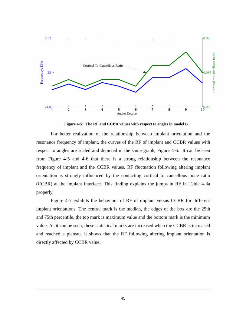
45
For better realization of the relationship between implant orientation and the
resonance frequency of implant, the curves of the RF of implant and CCBR values with
respect to angles are scaled and depicted in the same graph, Figure 4-6. It can be seen
from Figure 4-5 and 4-6 that there is a strong relationship between the resonance
frequency of implant and the CCBR values. RF fluctuation following altering implant
orientation is strongly influenced by the contacting cortical to cancellous bone ratio
(CCBR) at the implant interface. This finding explains the jumps in RF in Table 4-3a
properly.
Figure 4-7 exhibits the behaviour of RF of implant versus CCBR for different
implant orientations. The central mark is the median, the edges of the box are the 25th
and 75th percentile, the top mark is maximum value and the bottom mark is the minimum
value. As it can be seen, these statistical marks are increased when the CCBR is increased
and reached a plateau. It shows that the RF following altering implant orientation is
directly affected by CCBR value.
Figure 4-5: The RF and CCBR values with respect to angles in model B
1 2 3 4 5 6 7 8 9 1024.8
25
25.2
Angle: Degree
Fre
qu
en
cy
: K
Hz
1 2 3 4 5 6 7 8 9 100.08
0.085
0.09
Co
rtic
al
to C
an
cell
ou
s R
ati
o
Cortical To Cancellous Ratio

46
Table 4-3: Results of pig mandible
a. The RF of implant corresponding to the segment of pig mandible: KHz
Rotating angle (degree)
1 2 3 4 5 6 7 8 9 10
RF when Implant is
buried in the bone
12.18 12.21 12.02 11.98 12.03 12.09 12.72 12.98 12.87 12.94
RF when Implant is
moved 0.5 mm in
positive z-direction
9.86 9.88 9.76 9.7 9.81 10.07 9.85 9.8 9.84 9.6
RF when Implant is
moved 1mm in
positive z-direction
9.69 9.52 9.58 9.53 9.52 9.88 9.71 9.62 9.49 9.5
b. CCBR in segment pig mandible when the implant is moved 0.5mm in positive z-direction
CCBR 53.4 53.5 52.6 52.2 52.9 54.8 54 53.6 54 53.1
Figure 4-6: The RF and CCBR values with respect to angles in pig mandible model
1 2 3 4 5 6 7 8 9 109.5
9.6
9.7
9.8
9.9
10
10.1
Angle: Degree
Fre
qu
en
cy
: K
Hz
1 2 3 4 5 6 7 8 9 1052
52.5
53
53.5
54
54.5
55
Co
rtic
al
to C
an
cell
ou
s R
ati
oCortical to Cancellous Ratio

47
Figure 4-7: The behaviour of RF of implant versus CCBR for different implant orientations
4.3 DISCUSSION
To detect implant stability, various diagnostic analyses have been employed including
percussion test, standardized radiographs, cutting torque resistant analysis, reverse torque
test, and resonance frequency analysis (RFA) [8]. RFA method has recently became
popular because it is a noninvasive diagnosis method and the most accurate technique.
Atsumi et al. [8] classified the clinical applications of RFA including (1) a relation
between exposed implant length and resonace frequency or ISQ (Implant Stability
Quotient) values ;(2) differential interarch and intera-arch ISQ values for implants in
various locations (3) prognostic criteria for long term implant sucess; and (4) diagnostic
criteria for implant stability [54,30]. No study has been conducted to determine the
relation between the resonance frequency of implant and implant orientation.
In this study, by using FEA simulation, the relation between the RF of implant in an
optimal and comporomised orienation is identified. A three dimensional modelling
software is used and a 3D model of a pig mandible is constructed. Moreover, a simplified
epoxy cubical model is carried out to reduce the potential interference of heterogenousity
of adjucent structure in RF analyses. The effects of material properties, rotation and
contact area on the relation between RF of implant and implant orientation are
investigated in model A. The results demonstrates that in case only cortical or cancellous
0.09 0.1 0.12 0.14 0.16 0.19 0.21 0.24
24.9
24.95
25
25.05
25.1
25.15
CCBT
Res
on
ance
Fre
qu
ency
(K
Hz)

48
bone composes the bone, the effect of thsese paramaters are insignificant. Astrong
relation between implant orientation and RF of implant is found by depicting the curves
of the RF of implant and CCBR values with respect to angles (Figure 4-5 and 4-6). This
finding is also supported by the investigating the results of Figure 4-7 showing that the
RF of implant is increased in higher values of CCBR.
The RFs in model B where there is a thin layer of cortical bone is likely similar to the
RF values in model A when the entire contacting area is given by cortical bone. The
material properties of cortical bone are higher than cancellous bone material properties
(comparing 14 Gpa to 0.49 Gpa), so when the implant is interfaced with both cortical and
cancellous bone, even there is a thin layer of cortical bone, the RF of implant is mainly
influenced by hard tissue, not soft tissue.
In clinical applications, different individuals have different CCBR values. Therefore,
it is expected that each individual has a unique amount of RF of implant for a specific
orientation. As it can be realized in Figure 4-7, for a specific implant orientation, there is
a unique value for RF of implant depends on the CCBR value.
Figure 4-8 shows the mode shapes and their maximum deformations (DMX) for the
case of implant is buried in the bone and it rotates 1 degree around y-axis. The last mode,
No.18, is selected since the maximum amplitude of vibration happens at the implant.

49
Mode #: 11, Frequency: 7348 Hz, DMX=26
Mode #: 12, Frequency: 9091 Hz, DMX=34
Mode #: 13, Frequency: 9397 Hz, DMX=23
Mode #: 14, Frequency: 9740 Hz, DMX=22
Mode #: 15, Frequency: 10349 Hz, DMX=27
Mode #: 16, Frequency: 10789 Hz, DMX=31

50
Mode #: 17, Frequency: 11739 Hz, DMX=41
Mode #: 18, Frequency: 12175 Hz, DMX=42
Figure 4-8: The mode shapes of implant for the case of implant is buried in the bone and it is
rotates 1 degree around y-axis
4.4 CONCLUSION
In this study, we used the RFA method to determine the relation between implant
orientation and the resonance frequency of implant. A 3D modelling software is used to
construct a 3D model of a pig mandible from computed tomography images. Simplified
models (A & B) were also carried out to investigate the parameters concerning the
relation between RF changes and implant orienation in a simplified environment. It is
found that material properties, rotation, and contact area have minimum contribution to
the relation between implant orientation and RF of implant. We also found that the
resonance frequency of implant is changed and strongly influenced by the cortical to
cancellous bone ratio (CCBR) in interfacing areas of implant and bone. Based on the
results, the higher RF of implant happens at higher values of CCBR independent of angle.
In addition, by extruding the implant in positive z-axis in pig mandible model, we found
that the free length of implant influences the resonance frequency of implant. Increasing
the free length of implant resulted in decreasing the RF of implant. In conclusion, the computational results demonstrate the capability of RFA method in
determining the relation between implant orientation and resonance frequency of implant.

51
5: THE EFFECT OF SOFT TISSUE SURROUNDING THE
IMPLANT ON THE RESONANCE FREQUENCY OF
IMPLANT
As it is mentioned in chapter 1 implant stability depends on the successful
osseointegration. It is also mentioned in chapter 1 that the surrounding soft tissue plays
an important role in osseointegration of implant. When the implant is placed in the bone,
soft tissue forms in the contact surfaces between implant and bone. The regenerated soft
tissue at the implant/bone interface changes gradually to hard tissue during the process of
osseointegration. Failure cases happen when implant bone interface is not fully
osseointegrated or the hardened soft tissue at the interface fails (soft tissue forms at the
failure locations). Wang et al. [40] classified the tissue into three phases considering
different statuses of Osseointegration in the primary stability: the early healing phase
which is the first phase after implantation in which the callus (a new growth of osseous
matter at the ends of a fractured bone, serving to unite them) is composed of granulation
(fibrous connective tissue), the middle phase in which the fibrous tissue is predicted in
callus and the final tissue in which the cartilage (flexible connective tissue) is generated
[55]. Since the mechanical properties of all of these phases are softer than their
surrounding cortical and cancellous bone, hypothetically it is estimated that there is a
relation between the resonance frequency of implant and the soft tissue in the primary
stability. Wang et al [40] checked the relationships between the status of tissue and the
first/second resonance frequencies of the implant-tissue-bone system and found the
identifiable range of interfacial tissue of dental implants by means of resonance
frequency analysis.
This study aims to identify the effect of soft tissue surrounding the implant on RF of
implant using FEA simulation. MIMICS, a three dimensional (3D) modelling software is
used and a 3D model of a pig mandible is constructed from computed tomography (CT)

52
images. A vigorous parametric study is conducted to disclose the relation between RF of
implant and the surrounding soft tissue. Our analysis showed that the resonance
frequency of implant is significantly affected by soft tissue when it is formed in cortical
bone. In addition, the location and the size of soft tissue are two factors that influence the
RF of dental implant.
5.1 Materials and methods
5.1.1 The modelling of the pig jaw and soft tissue
A mandible of domestic young adult pig is obtained from a slaughter house and a
3.75 X 13 mm MIS endosseous implant is placed at the edentulous space between 1st
and 2nd
premolars by a dental implant surgion. MIS surgical protucole is followed to
place the implant so that primary stability of the implant is established in the bone. A 13
mm titanium abutment is torqued to the implant body at 32N/C . Due to the size
limitation of CT machine, the mandible is later block-sectioned at the premolar areas.
This section includes the implant, shown in Figure 4-1a. X-ray imaging of the sectioned
mandible is performed using a Kodak Cone Beam Computed Tomography unit (CBCT).
DICOM x-ray images were imported into MIMICS (version 14.12) to create an accurate,
3D model of the mandible, teeth and implant. To simplify the model and because of the
negligible affect of threads on our desired analysis the 3D dental implant model does not
include the thread portion. The model is later imported into finite element software,
ANSYS (version 12.1) for investigating RF analyses. In finite element analysis (FEA), a
physical system, such as the pig mandible model is converted into a number of discrete
elements and the properties of each element must be assigned from the bank of standard
reference data.
Individual tissue and structures were identfied in MIMICS from individual
DICOM images generated by CBCT using a default threshold technique. A radiologist
expert also confirmed and corrected the threshold criteria for the identifiable structures.
These structures included cancelous and cortical bone, enamel, dentine, and implant.
Cementum and dental pulp were excluded because of their relatively low volume and
thus minor effects on the analysis.
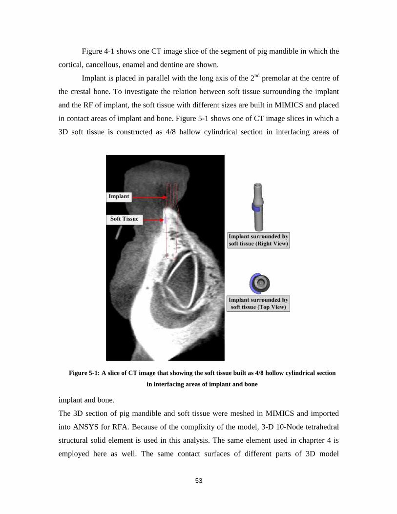
53
Figure 4-1 shows one CT image slice of the segment of pig mandible in which the
cortical, cancellous, enamel and dentine are shown.
Implant is placed in parallel with the long axis of the 2nd
premolar at the centre of
the crestal bone. To investigate the relation between soft tissue surrounding the implant
and the RF of implant, the soft tissue with different sizes are built in MIMICS and placed
in contact areas of implant and bone. Figure 5-1 shows one of CT image slices in which a
3D soft tissue is constructed as 4/8 hallow cylindrical section in interfacing areas of
implant and bone.
The 3D section of pig mandible and soft tissue were meshed in MIMICS and imported
into ANSYS for RFA. Because of the complixity of the model, 3-D 10-Node tetrahedral
structural solid element is used in this analysis. The same element used in chaprter 4 is
employed here as well. The same contact surfaces of different parts of 3D model
Figure 5-1: A slice of CT image that showing the soft tissue built as 4/8 hollow cylindrical section
in interfacing areas of implant and bone
54
(cortical, cancellous, enamel, dentine, soft tissue and implant) are all have to move
together to prevent the relative motion. Therefore, the coincident nodes are selected to be
rigidly fixed.
Material properties of different structures of this model are all assumed
homogeneous and isotropic. The material properties of cortical/cancellous bone, soft
tissue, enamel, dentine, and dental implant are listed in Table 5-1[40,53].
Table 5-1: Material properties of the partial pig jaw model
Young’s modulus E (Gpa) Poisson’s ratio Density
Cortical bone 14 0.3 1300
Cancellous bone 0.49 0.3 1300
Dental implant 104.8 0.342 4430
Enamel 75 0.33 2970
Dentine 15 0.31 2140
Soft tissue 0.17 1000
In the primary stability, the Young’s modolus of the soft tissue changes from 1MPa to 10 MPa [40]. In
this study, the Young’s modolus of soft tissue is assumed to be 10 MPa.
5.1.2 Parametric studies
5.1.2.1 The effect of the size
To detect the effect of size of soft tissue surrounding the implant on RFof implant,
3D soft tissue (2.5 mm tickness and 2 mm heigth) is built in MIMICS software in the
interfacing areas of implant and bone as an approximately 1/8 hollow cylindrical section
around the center of implant. The soft tissue increases from 1/8 to 8/8 hollow cylindrical
section in 1/8 increment, the tickness and the heigth of soft tissue remain constant for all
of these steps and the resonance frequencies of implant are analyzed. For better
monitoring of resonance frequency , the 3D soft tissue are also built as 12/13 and 23/24
hollow cylindrical section. Figure 5-2 shows tranverse and coronal views of one of CT
images slices when the soft tissue is constructed as 4/8 and 6/8 hollow cylindrical section

55
around the implant, the 3D models of soft tissue suroudning the implantt are also
depicted in Figure 5-2.
In addition, further analysis are carried out to investigate the effect of the size of
soft tissue on resonance frequency of implant. Hence, soft tissue is constructed as 2/8,
4/8, 6/8 and 8/8 hollow cylindrical section and the heigth of each case increases from 2
mm to 10 mm in 1 mm increment. The tickness of soft tissue remains constant for all of
these steps. Figure 5-3 shows 3D models of two differnt heigths of soft tissue when it is
built as 4/8 hollow cylindrical section.
5.1.2.2 The effect of location
In order to investigate the effect of location of soft tissue on resonance frequency
of implant, 3D soft tissue (2.5 mm tickness and 2 mm heigth) is built as 2/8 hollow
cylindrical section in contacting areas of implant and bone, shown in Figure 5-4, and the
the location of soft tissue is changed along negative z axis. In this case the soft tissue is
only interfcaed with cortical or cancellous. The resonance frequencies of implant is
analyzed in ANSYS simulation environment.

56
Figure 5-2: Transverse and coronal views of a slice of CT image showing the soft tissue as 4/8 and
6/8 hollow cylindrical section suroudnig the implant, and the 3D models of both implant and soft
tissues

57
Figure 5-3: 3D modesl of two different heigths of soft tissue when it is built as 4/8 hollow
cylindrical section.
Figure 5-4: 3D soft tissue is constructed as 2/8 hollow cylindrical section and is moved along z axis
Furthermore, the effect of the location of soft tissue on RF of implant is studied in
this chapter. To do so, a soft tissue as 1/8 hollow cylindrical section is counstructed and
rotated about z axis, as depicted in Figure 5-5. Two mode shapes, No.1 and No.2 are

58
investigated. In mode shapes No.1 and No.2, the implant rotates around x and y axis
repectively. The heigth (4 mm) and the tickness (2.5 mm) of soft tissue remain constant
for all directions shown as 1 to 8 in Figure5-5.
Figure 5-5: 3D soft tissue constructed as 1/8 hollow cylindrical section and rotates around z axis
5.2 Results
The resonance frequencies of implant when the soft tissue (2.5mm tickness and 2
mm heigth) is bulit as an approximtaley 1/8 hollow cylindrical section and increases from
1/8 to 8/8 are listed in Table 5-2 and plotted in Figure 5-6.
Table 5-2: The resonance frequencies corresponding to the soft tissue when it is built as an
apporximately 1/8 hollow cylindrical section and increases from 1/8 to 8/8: KHz
Segment of hollow cylindrical section
1/8 2/8 3/8 4/8 5/8 6/8 7/8 12/13 23/24 8/8
Resonnace
frequency of
implant (KHz)
11.11 11.1 11.078 11.065 11.033 10.936 10.916 10.9 10.895 10.099
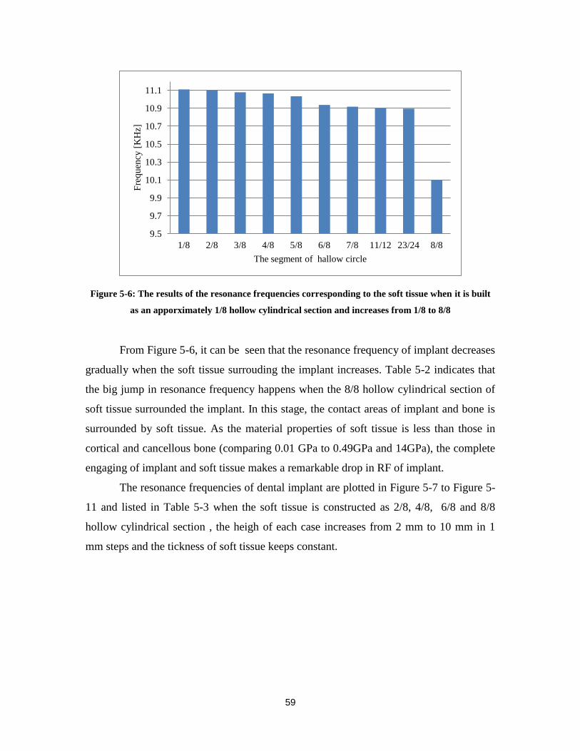
59
Figure 5-6: The results of the resonance frequencies corresponding to the soft tissue when it is built
as an apporximately 1/8 hollow cylindrical section and increases from 1/8 to 8/8
From Figure 5-6, it can be seen that the resonance frequency of implant decreases
gradually when the soft tissue surrouding the implant increases. Table 5-2 indicates that
the big jump in resonance frequency happens when the 8/8 hollow cylindrical section of
soft tissue surrounded the implant. In this stage, the contact areas of implant and bone is
surrounded by soft tissue. As the material properties of soft tissue is less than those in
cortical and cancellous bone (comparing 0.01 GPa to 0.49GPa and 14GPa), the complete
engaging of implant and soft tissue makes a remarkable drop in RF of implant.
The resonance frequencies of dental implant are plotted in Figure 5-7 to Figure 5-
11 and listed in Table 5-3 when the soft tissue is constructed as 2/8, 4/8, 6/8 and 8/8
hollow cylindrical section , the heigh of each case increases from 2 mm to 10 mm in 1
mm steps and the tickness of soft tissue keeps constant.
9.5
9.7
9.9
10.1
10.3
10.5
10.7
10.9
11.1
1/8 2/8 3/8 4/8 5/8 6/8 7/8 11/12 23/24 8/8
Fre
quen
cy [
KH
z]
The segment of hallow circle

60
Table 5-3: The resonanace frequencies corresponding to the soft tissue built as 2/8, 4/8, 6/8 and 8/8
hollow cylindrical section and the heigth of each case increases from 2 mm to 10 mm in
1 mm steps: KHz
Heigth of soft tissue (mm)
2 3 4 5 6 7 8 9 10
RF when soft tissue
is built as 2/8 circle
11.1 11.09 11.078 11.04 11.022 10.982 10.978 10.977 10.98
RF when soft tissue
is built as 4/8 circle
11.065 11.052 10.977 10.949 10.935 10.918 10.916 10.91 10.897
RF when soft tissue
is built as 6/8 circle
10.936 10.85 10.65 10.572 10.53 10.51 10.5 10.498 10.496
RF when soft tissue
is built as 8/8 circle
10.099 10.02 9.854 9.263 9.214 8.907 8.7 8.7 8.7
Figure 5-7: The results of the resonance frequencies of implant when the soft tissue is built as 2/8
hollow cylindrical section around the implant and the height of it increases from 2 mm to 10 mm
in 1 mm steps
10.96
10.98
11
11.02
11.04
11.06
11.08
11.1
11.12
2 3 4 5 6 7 8 9 10
Fre
quen
cy:
KH
z
The height of soft tissue: mm

61
Figure 5-8: The results of the resonance frequencies of implant when the soft tissue is built as 4/8
hollow cylindrical section around the implant and the heigth of it increases from 2 mm to 10 mm
in 1 mm steps
Figure 5-9: The results of the resonance frequencies of implant when the soft tissue is built as 6/8
hollow cylindrical section around the implant and the heigth of it increases from 2 mm to 10 mm
in 1 mm steps
10.88
10.9
10.92
10.94
10.96
10.98
11
11.02
11.04
11.06
11.08
11.1
2 3 4 5 6 7 8 9 10
Fre
quen
cy:
KH
z
The height of soft tissue: mm
10.4
10.5
10.6
10.7
10.8
10.9
11
2 3 4 5 6 7 8 9 10
Fre
quen
cy:
KH
z
The height of soft tissue: mm

62
Figure 5-10: The results of the resonance frequencies of implant when the soft tissue is built as 8/8
hollow cylindrical section around the implant and the height of it increases from 2 mm to 10 mm
in 1 mm steps
Figure 5-11: The results of the resonance frequencies of implant when the soft tissue is built as
2/8, 4/8, 6/8 and 8/8 hollow cylindrical section around the implant and the height of it increases
from 2 mm to 10 mm in 1 mm steps
From the plotted results of Figure 5-7 to Figure 5-11, it is figured out that the
resonance frequency of dental implant decreases significantly when the heigth of soft
tissue surrounding the implant increases from 2 mm to 7 mm and it reaches a plateaue
after 7 mm. In case the heigth of soft tissue is between 2 mm to 7 mm, the soft tissue is
8.4
8.6
8.8
9
9.2
9.4
9.6
9.8
10
10.2
2 3 4 5 6 7 8 9 10
Fre
quen
cy:
KH
z
The height of soft tissue: mm
8.4
8.9
9.4
9.9
10.4
10.9
2 3 4 5 6 7 8 9 10
Fre
quen
cy:
KH
z
The height of soft tissue: mm
2/8
4/8
6/8
8/8

63
essentially engaged with cortical bone while when it is between 7 mm to 10 mm the soft
tissue is interfaced with both cortical and cancellous bone. Therefore, the results indicate
that the RF of implant decreases considerbaly when the soft tissue is formed in cortical
bone. As it is shown in Figure 5-11 the resonance frequency of implant decreases mainly
when the whole contact areas of implant and bone are covered by soft tissue. Even
though in all cases the resonance frequency of implant decreases by increasing the heigth
of soft tissue surounding the implant in cortical bone, the substantial jump in resonnace
frequency happens when the whole contact area of implant and bone is surounded by soft
tissue. Comparing the mechanical properties of cortical (Young’s modolous of 14Gpa)
and cancellous (Young’s modolous 0.49 Gpa) to soft tissue (Young’s modolous of 0.01
GPa) indicates that the resonance frequency of implant is affected by its boundary
condtion material properties. Hence, in addition to the size of soft tissue, the location of
soft tissue is also an important factor in changing the RF of implant.
To precisely check the resonance frequencies reduction when the soft tissue is
built as 2/8, 4/8, 6/8 and 8/8 hollow cylindrical section, a variable is defined as the
absolute difference of the these frequencies by Eq.(5-1), and the values are listed in Table
5-4.
(i=1 to 4 , j=2 to 10) (5-1)
Where is the absolute differences of resonance frequecies;
and are the jth
frequency when the soft tissue is built as 2/8 (i=1), 4/8 (i=2), 6/8 (i=3), and 8/8 (i=4)
circle.
Table 5-4: The absolute differences of resonance frequencies corresponding to the soft tissue when it
is built as 2/8, 4/8, 6/8 and 8/8 circle and the heigth increases from 2 mm to 10 mm : Hz
2 3 4 5 6 7 8 9 10
RF of 4/8 compares to RF of 2/8 35 38 101 91 87 64 62 67 83
RF of 6/8 compares toRF of 2/8 164 240 428 468 492 472 478 479 484
RF of 8/8 compares to RF of 2/8 1001 1070 1224 1777 1808 2075 2278 2277 2280
From Table 5-4, it can be seen that the significant differences in resonance
frequency of implant occurs when the 8/8 hollow cylindrical section case is compared

64
with 2/8. It can be concluded that in clinical practice, any big change in RF of implant
implicates possiblity of growing soft tissue in contacting areas of implant and bone.
The resonance frequencies of implant in case of the soft tissue (thickness 2.5 mm
and height 2 mm) is constructed as 2/8 hollow cylindrical section and the location of it
moves along negative z axis, Figure 5-4, are listed in Table 5-5 and plotted in Figure 5-
12.
Table 5-5: The resonance frequencies corresponding tothe soft tissue when it is built as 2/8 hollow
cylindrical section and moves along z axis, Fig. 7: KHz
45.8-
43.8
43.8-
41.8
42.8-
40.8
41.8-
39.8
40.8-
38.8
39.8-
37.8
38.8-
36.8
37.8-
35.8
35.8-
33.8
Resonance frequency 11.1 11.02 11.015 11.007 10.95 10.959 10.965 10.978 10.975
Figure 5-12: The resonance frequencies of the soft tissue when it is built as 2/8 hollow cylindrical
section and moves along z axis, : KHz
The Figure 5-12 shows that the RF of implant decreases significanly at the border
of cortical and cancellous bone. When the soft tissue is formed in cortical bone, the

65
effectiveness of soft tissue in decreasing the RF of implant is more visiable than when it
is formed in cancellous bone.
The resonance frequencies of implant are listed in Table 5-6 and shown in Figure
5-13 when the soft tissue is constructed as 1/8 hollow cylindrical section and rotates
around the center of implant, shown in Figure 5-5. In Figure 5-13, the dash line are the
mode shapes No.1 and the solid line are the mode shapes No.2. Figure 5-13 shows that
the resonance frequencies of implant for the mode shapes that are related to the dash line
are higher than those that are related to the solid line. Furthermore, Figure 15 indicates
that the direction of soft tissue around the implant will not affect the resonance frequency
of implant considerably. For example, when the soft tissue is located in direction 1 and
moved to location 2 (Figure 5-5) , the RFs of implant for the mode shape No.1 are 10.912
KHz and 11.102 KHz repectively.
Table 5-6: The perpendicular resonance frequencies corresponding tothe soft tissue when it is built
as 1/8 circle and rotates around the center of implant: KHz
Direction
1 2 3 4 5 6 7 8
Implant rotates around y axis 8.798 8.911 8.957 8.853 8.897 8.956 8.772 8.835
Implant rotates around x axis 10.912 11.102 11.082 11.032 10.959 11.125 10.902 10.98

66
Figure 5-13: The resonance frequencies of the soft tissue when it is built as 1/8 hallow circle and
rotates around the center of implant, shown in Figure 5-6: KHz
Figure 5-14 and Table 5-7 show the results of resonance frequencies when the
soft tissue (2.5 mm tickness) is formed as 2/8 circle and the heigth of it increases from 2
mm to 10 mm. This is the exactly the same as the case shown in Figure 5-8, but since it is
found that the RF of implant decreases when the soft tissue is formed in cortical and
reaches a platuea when it grows to cancellous bone, some new cases have been added in
the border of cortical to cancellous to better clarify what happens there. When the heigth
of soft tissue is 7.8 mm, the soft tissue is fully located in cortical bone and at 8 mm it is
engaged with both cortical and cancellous bones.
Table 5-7: The resonance frequencies of implant in case the soft tissue is constructed as 2/8 circle and
the heigth of it increases from 2 mm to 10 mm:KHz
Heigth of soft tissue (mm)
2 3 4 5 6 7 7.8 8 8.6 9 9.4 10
RF of
implant
11.1 11.09 11.078 11.04 11.022 10.982 10.98 10.978 10.977 10.977 10.978 10.98

67
Figure 5-14: The results of resonance frequencies of the soft tissue built as 2/8 circle and the
height of it increases from 2 mm to 10 mm
5.3 Discussion
In this study, we used the RFA method to determine the effect of soft tissue
surrounding the implant on RF of implant. We found that the resonance frequency of
implant is influenced by the size and the location of soft tissue especially when it is
formed in cortical bone.
From the calculated results in Figure 5-6 to Figure 5-11 it can be seen that when the
soft tissue is formed in cortical bone, the resonance frequency of implant is mainly
affected by the size of soft tissue,. When the soft tissue becomes larger in cortical, the
resonance frequency decreases significantly but when it passes the border between
cortical and cancellous and continues to grow in cancellous bone, the resonance
frequency remains constant and reaches a plateau. Theoretically, the resonance frequency
of a cantilever beam fixed at one side and free to vibrate at the other end is directly
related to the boundary condition variation. This observation can be explained by
considering the material properties of cortical, cancellous and soft tissue. It is known that
the cortical bone is more rigid than both cancellous and soft tissue (cancellous is harder
than soft tissue). Thus, more flexibility in implant-bone integration can be expected when
the soft tissue is formed in cortical bone than when it is formed in cancellous bone
(Figure 5-12). The lowest resonance frequency in Figure 5-12 happens at the border of
10.96
10.98
11
11.02
11.04
11.06
11.08
11.1
11.12
2 3 4 5 6 7 7.8 8 8.6 9 9.4 10
Fre
quen
cy:
KH
z
The height of soft tissue: mm

68
cortical to cancellous bone. The results are in agreement with the results of [56]. They
investigated the effect of foundation flexibility on seismic response of reinforced
concrete TV-towers and found that the foundation flexibility increases the natural
periods, alters the natural mode shapes, and decreases the base bending moment.
5.4 Conclusion
The FEA results indicate that RF of implant decreases because of formation of soft
tissue at the implant-bone interface. The RF of implant decreases considerably when soft
tissue grows in cortical bone. Moreover, it is found that the RF of implant is not very
sensitive to the formation of soft tissue in cancellous bone. Finally, the direction of soft
tissue formation in a dental implant does not affect its RF.

69
6: EXPERIMENTS ON PIG JAW
In numerical approach, we assumed that the material properties of the bone and tissue
are all homogenous and isotropic which might not necessarily valid in reality. To observe
these effects, in vivo studies is carried out in this chapter. The effect of free length of
implant on RF has been studied in previous chapters both experimentally (implant placed
in a chuck) and numerically (FE method). In this chapter, the effect of some parameters
such as free length, and size on RF is investigated. For these experiments, three domestic
young adult pig mandibles were obtained from the slaughter house (Britco Pork Inc.). A
3.75×11.5 mm MIS endosseous implant is placed in pig mandible No.1. Two different
implant sizes, 3.75×13 mm and 4.2×10 mm, are placed in the right and left sides of pig
mandible No.2. The last pig mandible is used for placing 3.75×13 mm implant. MIS
surgical protocol is followed to place the implants to establish the primary implant
stability. In this in vivo analysis, implant is buried in the bone and the ‘transfer mount’ is
screwed into implant. The implant is excited by an impulse hammer (Dynapulse model
5800B2, Dytran Instruments Inc., USA). The vibrating signal is recorded by an
accelerometer (model 3035BG). A non-contact acoustic microphone (40BE repolarised
free field microphone, G.R.A.S sound and vibration, Denmark) is also used to measure
impact sound. Both impulse force and the vibrating signal response are transferred to
Photon Software for modal analysis. The in vivo test set up components including pig
mandible, transfer mount, accelerometer, microphone and Photon are shown in Figure 6-
1.

70
Figure 6-1: In vivo test set up
6.1 The effect of implant’s free length on RF
The effect of implant’s free length on RF is analyzed by using both accelerometer
and microphone.
6.1.1 Accelerometer results
The accelerometer is used for recording the vibrating response. The tests are
repeated three times, and each test is the average of five impacts. In pig mandibles NO.1
three different implant’s free lengths (1.78 mm, 2.29 mm and 2.87mm) are studied. The
FFT (Fast Fourier Transform) of vibrating signals are shown in Figure 6-2.

71
Figure 6-2: The FFT of different free length of implant in pig No.1
The results shows that the RF decreased from (6.8) KHz to (5.84) KHz when the
length of implant left out of the bone increased from 1.78 mm to 2.87 mm respectively.
It can be concluded that the RF of implant decreases with increasing the free length.
The same conclusion is obtained by studying the effect of free length on the RF of
implant in pig mandible NO.2. Two implants (3.75×13 mm and 4.2×10 mm) are placed
in the right and left side of the jaw respectively. In these experiments the jaw is fixed by a
metal clamp from the opposite side where the implant is placed and the RF is measured
for both implants at different free lengths. The results are tabulated in Table 6-1.
0 2000 4000 6000 8000 10000 12000 14000 16000-40
-30
-20
-10
0
10
20
30
Frequency (Hz)
1.78 mm
2.29 mm
2.87 mm
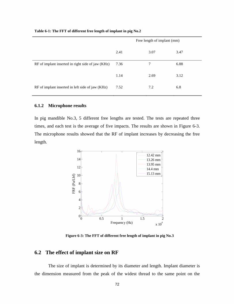
72
Table 6-1: The FFT of different free length of implant in pig No.2
Free length of implant (mm)
2.41 3.07 3.47
RF of implant inserted in right side of jaw (KHz) 7.36 7 6.88
1.14 2.69 3.12
RF of implant inserted in left side of jaw (KHz) 7.52 7.2 6.8
6.1.2 Microphone results
In pig mandible No.3, 5 different free lengths are tested. The tests are repeated three
times, and each test is the average of five impacts. The results are shown in Figure 6-3.
The microphone results showed that the RF of implant increases by decreasing the free
length.
Figure 6-3: The FFT of different free length of implant in pig No.3
6.2 The effect of implant size on RF
The size of implant is determined by its diameter and length. Implant diameter is
the dimension measured from the peak of the widest thread to the same point on the
0 0.5 1 1.5 2
x 104
0
2
4
6
8
10
12
14
16
Frequency (Hz)
FR
F (
Pa/
Lb
f)
12.42 mm
13.26 mm
13.95 mm
14.4 mm
15.13 mm

73
opposite side of the implant. Currently available implants vary in diameter from 3 to 7
mm. The requirements for implant diameter are based on both surgical and prosthetic
requirements. Implant length is the dimension from the platform to the top of implant. It
has been an axiom in implant dentistry that longer implants guarantee better success rates
and prognosis. Although a linear relationship between length and success rate has not
been proven, studies have shown that shorter implants have statistically lower success
rates [57].
The effect of implant size on RF is analyzed in this section. Both implants buried in
the left and right sides of pig mandible No.2, are excited by impulse hammer and the
vibration signals are collected by the accelerometer and analyzed by Photon. The results
showed that the size of implant is one of the factors that influence the RF. The In
summary, the longer implant showed higher RF. In this analysis the RF of implant placed
in the right side of pig jaw (3.75×13 mm), is approximately 8 KHz and the RF for the left
side implant (4.2×10 mm) is 7.7 KHz.
6.3 Comparison between the RF of implant inserted in a segment and
whole pig mandible
The pig mandible No.2 is cut and a segment of it is included the implant (see Figure
6-4) is tested. The same method used for other tests is used to acquire the RF. The RF for
the whole and partial pig mandibles are shown in Figure 6-4. As it is shown in the Figure
6-4, the RF of implant is the same in both cases. This finding is useful for justifying
model reduction in FEM analysis. Comparing with the whole mandible, the segment pig
mandible has less number of nodes and elements and thus the analyzing process will be
faster.

74
Figure 6-4: Comparison between the RF of implant in selected and whole pig mandible

75
7: EXPERIMENTAL STUDIES TO FIND THE EFFECT OF
SURROUNDING SOFT TISSUE ON RF OF IMPLANT
Soft tissue is a body part that connects, supports, or surrounds other structures and
organs of the body, excluding bone. The influence of soft tissues, joints and the fibula on
the human tibia’s natural frequency have been reported by Van der Perre et al. [58,59]
and Cornelissen et al. [60,61]. They concluded that the major factors that influence the
results was the mass and damping effect of muscles. Tsuchikane et al. [62] investigated
the influence of joints and soft tissue on the RF of the human tibia using the impulse
response method combined with modal analysis. Their findings indicate that soft tissue,
joint and fibula play a role in damping vibration. They suggested that a change in the RF
of the tibia represents a change in the condition of the tibia itself. In dental applications, it
is expected that soft tissue affects the RF of implant and little is known about this effect.
In this chapter, an experimental study is conducted to investigate the influences of
the surrounding soft tissue on the RF of the implant. It is found that the RF of implant
decreases when it is surrounded by soft tissue. Moreover, the results show that the angle
between the direction of excitation and the location of soft tissue affects the RF.
7.1 Material and Methods
As shown in Figure 7-1a, a 3.75×11.5 mm MIS endosseous implant is fixed by a
rotating metal chuck stand, capable of rotating 360 degree about its’ center. A piece of
rubber is attached to the dental implant to represent the effect of soft tissue (similar to
soft tissue, rubber is both elastic and viscous). As depicted in Figure 7-1, rubber adheres
perfectly to the implant. The implant is excited by an impulse force applied by an
inverted pendulum. To improve the quality of impact forces, a conical impact tip is
fabricated and installed. The impact force applied to the implant is measured by a force
sensor (Dytran model 1022V) inserted at the end of the device. The intensity of transient

76
force remains constant for all tests since the pendulum is released at the same height for
all experiments. When the impact head hits the implant, the force sensors triggers the
impact and the microphone begins collecting acoustic signal. Here, all the tests are
repeated three times when the chuck is rotated about its center from 00 to 360
0 (Figure 7-
1c) in 100 increments. Each incremental rotation of the chuck changes the angle between
the direction of impact force and the location of the rubber. The FRF of the microphone
signals are calculated by a program written in MATLAB. The sharp peak of the FRF
shows the resonance frequency of the implant. The test is also repeated when the rubber
is removed and the implant is in fully contacted with the metal chuck.
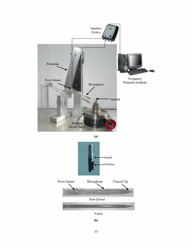
77
(a)
(b)

78
(c)
Figure 7-1: Test set up
7.2 Results
Figure 7-2a and b show a sample FRF of the microphone with and without rubber
for the angle 1000.
The RFs of implant when the chuck is rotated from 00 to 360
0 around its centre in
100 increments are depicted in Figure 7-3. The minimum, maximum, mean value and
standard deviation are shown in this figure. The tests with the rubber is indicated by a
dash line, and the tests without the rubber are shown by a solid line.
The results show that the RF of implant decreases when the rubber is attached.
For the case with the rubber, the RF at 1000 has a mean value of 7.88 KHz, and 9 KHz
when fully interfaced with the metal chuck. As it is shown in Figure 7.4, the mean value
of RF of implant when it has the rubber is approximately 8.1 KHz while it is 8.77 KHz
without it. From Figure 7-3 it can be seen that the difference between the RF of implant,
with and without rubber at certain degrees are bigger. At these angles, the angle between
the direction of impact and the location of the soft tissue are much closer than other
angles. When the rubber and impact are in the same direction, the implant has lower RF
compared to other angles.

79
(a)
(b)
Figure 7-2: (a) FRF of microphone when the soft tissue is removed and the implant is contacted
with metal chuck (b) FRF of microphone when the soft tissue is adhered to the implant and the
chuck is rotated 1000 around its centre
0 0.5 1 1.5 2 2.5 3 3.5 4
x 104
0
1
2
3
4
5
6
7
Frequency (Hz)
FR
F (
Pa/
Lb
f)
0 0.5 1 1.5 2 2.5 3 3.5 4
x 104
0
2
4
6
8
10
12
Frequency (Hz)
FR
F (
Pa/
Lb
f)

80
Figure 7-3: The RFs of implant when the chuck is rotated from 00 to 360
0 around its centre in 10
0
increments
Figure 7-4: The mean values of RFs of implant when the chuck is rotated from 00 to 360
0 around
its centre in 100 increments
7.3 Conclusion
The influences of the surrounding soft tissue on the RF of implant are investigated
using the impulse response method.
It is shown that the soft tissue influences the RF. This finding suggests that a
change in the RF of an implant represents a change in the boundary condition. The results
also demonstrate that the RF is mainly affected by the angle between the direction of the
0 50 100 150 200 250 300 3507000
8000
9000
10000
Rotating Angle (Degree)
RF
(H
z)
Without Rubber
With Rubber
7600
7800
8000
8200
8400
8600
8800
9000
Without Rubber With Rubber
Fre
quen
cy (
Hz)

81
impact and the location of the soft tissue. When the soft tissue and the impact force are in
the same direction, the RF is the lowest. This finding could be used in dental application
to predict approximately the location of defect in bone implant integration.

82
8: CONCLUSIONS AND RECOMMENDATIONS
In order to develop techniques and strategies for assessing dental implant stability
numerical modelling is a strong method that has been widely used in recent years. In this
thesis, both experimental and numerical results show that the resonance frequency of a
coupled implant/chuck is influenced by the material property of each individual units as
well as the quality of their integration. Moreover, it is found that the RF of the implant
increases when the implant and bone are more integrated, and RF reaches to a plateau
when the implant-bone interface is fully integrated.
We also found that the resonance frequency of implant is strongly influenced by
the cortical to cancellous bone ratio (CCBR) in the interfacing areas of implant and bone.
The computational results also confirm that RF method is useful in determining
the effect of soft tissue on implant stability. It is shown that the resonance frequency of
implant decreases considerably when soft tissue volume grows in the cortical bone.
Moreover, it is found that the resonance frequency of implant is not sufficient sensitive
when the soft tissue is formed in cancellous bone. Experimental results show the
remarkably influence of soft tissue on RF of an implant. This finding suggests that a
change in the RF of an implant represents a change in the boundary condition of the
bone. The results also demonstrate that the RF is mainly affected by the angle between
the direction of the transient force and the location of the soft tissue.
In addition, the size of implant is shown to have an important role in determining
the RF of implant. It is found that, the resonance frequency of implant is increases when
the free length of implant is decreased.
The usability of this method is applicable not only to dental implant but to also
other categories of implant such as hip implant to check the stability of implant and
realize the integration process. In general, the results of this study can be insightful for

83
future research. For the future works, it is possible to integrate the 3D pig jaw model in
order to investigate the effect of some parameters such as material properties of bone on
RF of implant.
.

84
9: REFERENCE LIST
1. Capek L, Simunek A, Slezak R, Dzan L (2009) Influence of the orientation of the
Osstell® transducer during measurement of dental implant stability using
resonance frequency analysis: A numerical approach. Med Eng Phys 31:764–9
2. Poul Holm-Pedersen, Niklaus P.Lang, Frauke Muller (2007) What are the
longevities of teeth and oral implants? Clin. Oral Impl. Res. 18:15-19
3. Koller B, Att W, Strub JR (2011) Survival rates of teeth implants and double
crown-retained removable dental prostheses systematic literature review. Int J
Prosthodont 24:109-17
4. Chung WE, Rubestien JE, Phillips KM, Raigrodski AJ (2009) Outcomes
assessment of patients treated with osseointegrated dental implants at the
university Washington Graduate Prosthodontic Program,1988 to 2000. Int J Oral
maxillofac Implants 24:927-35
5. Brunski JB. (1992) Biomechanical factors affecting the bone-dental implant
interface. Clin Mater 10:153-201
6. Sennerby L, Roos J. (1998) Surgical determinants of clinical success of
osseointegrated oral implants: A review of the literature. Int J Prosthodont
11:408-20
7. Jensen O. (1994) The carter hypothesis. In: Burser D, dahlin C, Schenk RK(eds).
Guided bone regeneration in implant dentistry. Hong Kong:Quintessence,
238:239
8. Mihoko Atsumi, Sang-Hoon Park, Hom-Lay Wang (2007) Methods used to assess
implant stability status. The International Journal of Oral & Maxillofacial
Implants 22:743-754
9. Meredith, N., Shagaldi, F., Alleyne, D., Sennerby, L., Cawley, P. (1997) The
application of resonance frequency measurements to study the stability of
titanium implants during healing in the rabbit tibia. Clinical Oral Implants
Research 8:234–243
10. Hermann JS. , Schoolfiled JD, Nummikoski PV., Buser D, Schenk RK, Cichran
DL (2001) Crestal bone changes around titanium implants: a methodology study
comparing linear radiographic with histometric measurements. Int J Oral
Maxillofac Implants 16:475-85
11. Goodson JM,Haffajee AD, Socransky SS. (1984) The relationship between
attachment level loss and alveolar bone loss. J Clin Periodontol 11:384-359
12. Johansson P, Strid K (1994) Assessment of bone quality from cutting resistance
during implant surgery. Int J Oral Maxillofac Implants 9:279-288

85
13. Friberg B, Sennerby L, Roos J, Johansson O, Strid CG, Lekholm U (1995)
Evaluation of bone density using cutting resistance measuremnts and
microradiography: An in vitro study in pig ribs. Clin Oral Implants Res 6:164-171
14. Roberts WE, Smith RK, Zilberman Y, Mozsary PG, Smith RS (1984) Osseous
adaption to continuous loading of rigid endosseous implants. Am J Orthod. 86:95-
111
15. Sullivan DY, Sherwood RL, Collins TA, Krogh PH. (1996) The reverse torque
test: A clinical report. Int J Oral Maxillofac Implants 11:179-185
16. Lim S, Cha J, Hwang C. (2008) Insertion Torque of Orthodontic Miniscrews
According to Changes in Shape, Diameter and Length. Angle Orthod 78:234-240
17. Turkyilmaz I, Tumer C, Ozbek E, Tozum T. (2007) Relations between the bone
density values from computerized tomography, and implant stability parameters: a
clinical study of 230 regular platform implants. J Clin Periodontol 34:716-722
18. Kaneko T. (1991) Pulsed oscillation technique for assessing the mechanical state
of the dental implant-bone interface. Bio-materials 12:555-560
19. Kaneko T,Nagai Y, Ogino M, Futami T, Ichimura T (1986) acoustoelastic
technique for assessing the mechanical state of the dental implant-bone interface.
J Biomed Mater Res 20:169-176
20. Aoki H (1987) The mobility of healthy teeth as measured with the impact hammer
method. Kanagawa Shigaku 22:13-31
21. Hirakawa W (1986) An attempt to measure tooth mobility in terms of time
domain wave forms. Kanagawa Shigaku 21:529-543
22. Matsuo E, Hirakawa K, Hamada S. (1989) Tooth Mobilitt measuremet technique
using ECM impact hammer method. Bull Kanagawa Dent Coll 17:9-19
23. Manz M, Morris H, Ochi S. (1992) An evaluation of the Periotest system. Part I:
Examiner reliability and repeatability of readings. Imp Dent 1:142-146
24. Salvi G, Lang N. (2004) Diagnostic parameters for monitoring peri-implant
conditions. Int J Oral Maxillofac Implants 19:116-127
25. N. Meredith, D. Alleyne, P. Cawley (1996) Quantitative determination of the
stability of the implant-tissue interface using resonance frequency analysis. Clin
Oral Impl Res 7: 261-267
26. Huwiler MA, Pjetursson BE, Bosshardt DD, Salvi GE, Lang NP (2007)
Resonance frequency analysis in relation to jawbone characteristics and during
early healing of implant installation. Clin Oral Impl Res 18:275–80
27. Tozum TF, Turkyilmaz I, Yamalik N, Karabulut E, Eratalay K (2007) Analysis of
the potential association of implant stability, laboratory, and image-based
measures used to assess osteotomy sites: early versus delayed loading. J
Periodontol 78:1675–82
28. Meredith, N., Book, K., Friberg, B., Jemt, T., Sennerby, L. (1997) Resonance
frequency measurement of implant stability in vivo. A cross-sectional and

86
longitudinal study of resonance frequency measurements on implants in the
edentulous and partially dentate maxilla. Clinical Oral Implants Research 8:226–
233
29. Bischof, M., Nedir, R., Szmukler-Moncler, S., Bernard, J.P., Samson, J. (2004)
Implant stability measurement of delayed and immediately loaded implants
during healing. Clinical Oral Implants Research 5:529–539.
30. Glauser, R., Sennerby, L., Meredith, N., Ree, A., Lundgren, A., Gottlow, J., Ha¨
mmerle, C.H.F. (2004) Resonance frequency analysis of implants subjected to
immediate or early functional occlusal loading. Clinical Oral Implants Research
15:428–434
31. Rasmusson,L., Meredith,N., Cho, H.I. & Sennerby (1999) The influence of
simultaneous versus delayed placement on the stability of titanium implants in
onlay bone grafts: a histologic and biomechanics study in the rabbit. International
Journal of Oral and maxillofacial Surgery 28:224-231
32. Huang, H.M., Chiu, C.L., Yeh, C.Y., Lin, C.T., Lin, L.H., Lee, S.Y. (2003) Early
detection of implant healing process using resonance frequency analysis. Clinical
Oral Implants Research 14:437–443
33. Huang, H.M., Cheng, K.Y., Chen, C.H., Lin, C.T., Lee, S.Y. (2005) Design of a
stability-detecting device for dental implants. Proceedings of the Institution of
Mechanical Engineering—Part H—Journal of Engineering in Medicine 219:203–
211
34. Huang, H.M., Pan, L.C., Lee, S.Y., Chiu, C.L., Fan, K.H., Ho, K.N. (2000)
Assessing the implant/bone interface by using natural frequency analysis. Oral
Surgery, Oral Medicine, Oral Pathology, Oral Radiology, and Endodontics 90:
285–291
35. Lee SY, haung HM, Lin CY,Shih YH (2000) In vivo and in vitro natural
frequency analysis of peridontal conditions: An innovative method. J Periodontol
71:632-640
36. Huang HM, Chiu CL,Yeh CY, Lee SY (2003) Factors influencing the resonnace
frequency of dental implants. J Oral Maxillofac Surg 61:1184-1188
37. Huang HM, Lee SY, Yeh CY, LIn CT (2002) Resonnace frequency assessemnt of
dental implant stability with various bone qualities: A numerical approach. Clin
Oral Implants Res 13:65-74
38. Zix J, Hug S, Kessler-Liechti G, Mericske-Stern R (2008) Measurement of dental
implant stability by resonance frequency analysis and damping capacity
assessment: comparison of both techniques in a clinical trial. Int J Oral Maxillofac
Implants 23:525-530
39. Williams, K.R. & Williams, A.D.C. (1997) Impulse response of a dental implant
in bone by numerical analysis. Biomaterials 18: 715–719
40. S. Wang, G.R. Liu, K.C. Hoang, Y. Guo (2011) Identifiable range of
osseointegration of dental implants through resonance frequency analysis. Med
Eng Phys 32:1094–1106.

87
41. De Almeida, M. S., Maciel, C. D., and Pereira, J. C. (2007) Proposal for an
ultrasonic tool to monitor the osseointegration of dental implants. Sensors
7:1224–1237
42. Mathieu, V., Anagnostou, F., Soffer, E., and Haiat, G. (2011a) Ultrasonic
evaluation of dental implant biomechanical stability an in vitro study. J. Acoust.
37:262–270
43. Daniel Inman (2008) Engineering Vibration. 3rd
edition Pearson, Prentice Hall.
44. Ewins (2000) Modal testing : theory, practice and application. 2nd
edition
Research Studies Press .
45. Meredith N. (1998) Assessment of implant stability as a prognostic determinant.
Int J Prosthodont 11:491-501
46. Meredith, N., Shagaldi, F., Alleyne, D., Sennerby, L., Cawley, P. (1997) The
application of resonance frequency measurements to study the stability of
titanium implants during healing in the rabbit tibia. Clinical Oral Implants
Research 8:234–243
47. Thomson, W.T., (1988) Free vibration. In: Thomson, W.T., ed. Theory of
Vibration with Applications, 3rd edition. New York: Prentice-Hall Inc.
48. Lindh T, Gunne J, Tiliberg A, Molin M. (1998) A meta-analysis of implants in
partial edentulism. Clin Oral Implants Res 9; 80- 90
49. Holm-Pedersen P, Lang Np, Muler F. (2007) What are the longevities of teeth and
oral implants? Clin Oral Implants Res 18:1 5-19
50. Pjetursson BE, Tan K, Lang NP, Bragger U, Egger M, Zwahlen M. (2004) A
systematic review of the survival, and complication rates of fixed partial dentures
(FPDs) after an observation period of at least 5 years- Implant-supported FPDs.,
Clin Oral implants Res 15:625-642
51. Eduardo Piza Pellizzer Pellizzer EP, Falcón-Antenucci RM, de Carvalho PS,
Sánchez DM, Rinaldi GA, de Aguirre CC, Goiato MC (2011) Influence of
Implant Angulation With Different Crowns on Stress Distribution. The Journal of
Craniofacial Surgery 22:434-437
52. Roberto Sorrentino, Enrico Felice Gherlone, Gaetano Calesini, Fernando Zarone
(2010) Effect of Implant Angulation, Connection Length, and Impression
Material on the Dimensional Accuracy of Implant Impressions: An In Vitro
Comparative Study. Clinical Implant Dentistry and Related Research 12:63-76
53. Integrated Biomaterial Science, edited by R. Barbucci. Kluwer academic/Plenum
publishers, New York, 2002
54. Ernsanli S, Karabuda C, Becj F, Leblebicioglu B. (2005) Resonance frequency
analysis of one-stage dental implant stability during the Osseointegration period. J
Peridontol 76:1066-1071
55. Lacroix D, Prendergast PJ, Li G, Marsh D. (2002) Biomechanical model to
simulate tissue differentiation and bone regeneration: application to fracture
healing. Med Biol Eng Comput 40:14-21

88
56. A. Halabian, M.H. El Naggar (2001) Effect of foundation flexibility on seismic
response of reinforced concrete TV-towers. Can. J. Civ. Eng. 28:465-481
57. Winkler S, Morris HF, Ochi S. (2005) Implant survival to 36 months as related to
length and diameter. Ann Periodontol 5:22-31
58. Van der Perre, G., Van Audekercke, R, Martens, M. and Mulier, J. C. (1983)
Identification of the in uivo vibration modes of human tibiae by modal analysis.
J. Biomech. Engng, 105:244-248
59. Van der Perre, G. and Cornelissen, P. (1983) On the mechanical resonance of
human tibia in vivo. J. Biomechanics 16:549-552
60. Cornelissen, M., Cornelissen, P. and Van der Perre, G. (1982) A dynamic model
for a healing fractured tibia. In Biomechanics: principles and applications (Eds R.
Huiskes, D. H. Van Campen and J. R. DeWijn) 213-218 (Martinus Nijhoff, The
Hague).
61. Cornelissen, M., Van der Perre, G., Martens, G. and Mulier, J. C. (1984)
Vibration measurements correlated with mechanical stability characteristics. In
Advances in biomaterials, biomechanics and biomaterials 83 (Eds P. Ducheyne,
G. Van der Perre and A. Aubert) 127-132 (Elsevier, Amsterdam).
62. Tsuchikane A, Nakatsuchi Y, Nomura A. (1995). The einfluence pf joints and soft
tissue on the natural frequency of the human tibia using the impulse response
method. Proc Instn Mech Engrs 209:149-155