Embed Size (px)
Citation preview
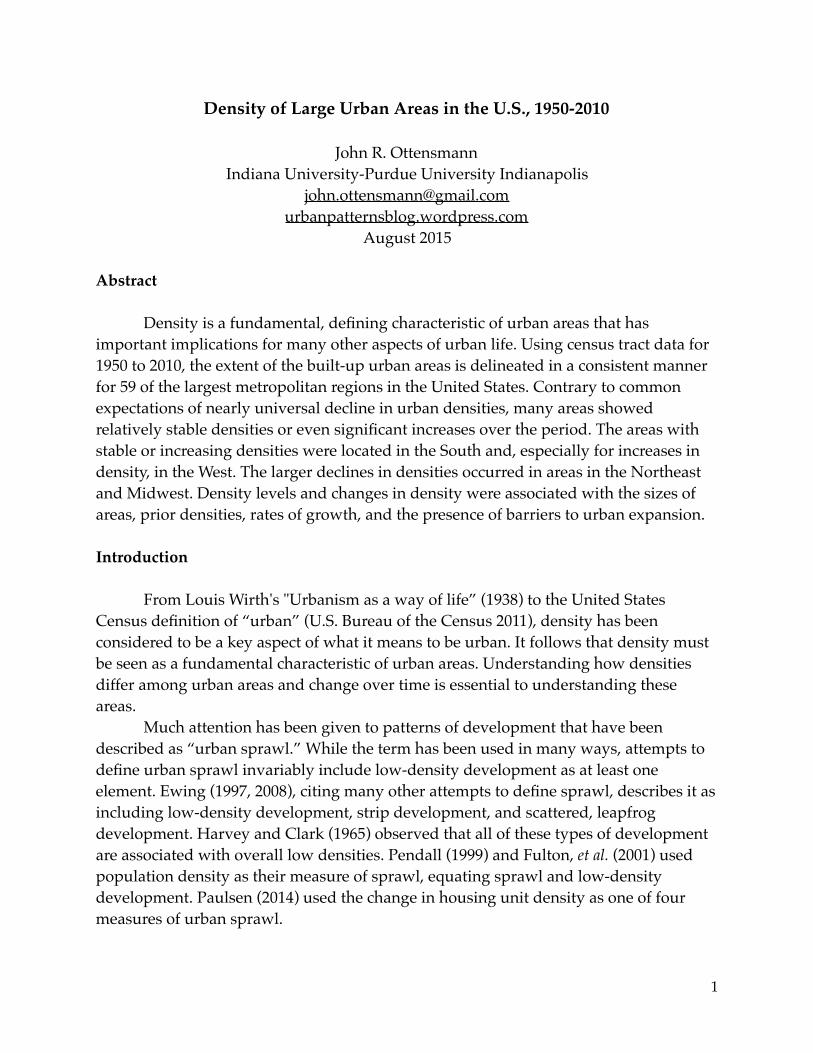
Density of Large Urban Areas in the U.S., 1950-2010
John R. OttensmannIndiana University-Purdue University Indianapolis
August 2015
Abstract
Density is a fundamental, defining characteristic of urban areas that has important implications for many other aspects of urban life. Using census tract data for 1950 to 2010, the extent of the built-up urban areas is delineated in a consistent manner for 59 of the largest metropolitan regions in the United States. Contrary to common expectations of nearly universal decline in urban densities, many areas showed relatively stable densities or even significant increases over the period. The areas with stable or increasing densities were located in the South and, especially for increases in density, in the West. The larger declines in densities occurred in areas in the Northeast and Midwest. Density levels and changes in density were associated with the sizes of areas, prior densities, rates of growth, and the presence of barriers to urban expansion.
Introduction
From Louis Wirth's "Urbanism as a way of life” (1938) to the United States Census definition of “urban” (U.S. Bureau of the Census 2011), density has been considered to be a key aspect of what it means to be urban. It follows that density must be seen as a fundamental characteristic of urban areas. Understanding how densities differ among urban areas and change over time is essential to understanding these areas.
Much attention has been given to patterns of development that have been described as “urban sprawl.” While the term has been used in many ways, attempts to define urban sprawl invariably include low-density development as at least one element. Ewing (1997, 2008), citing many other attempts to define sprawl, describes it as including low-density development, strip development, and scattered, leapfrog development. Harvey and Clark (1965) observed that all of these types of development are associated with overall low densities. Pendall (1999) and Fulton, et al. (2001) used population density as their measure of sprawl, equating sprawl and low-density development. Paulsen (2014) used the change in housing unit density as one of four measures of urban sprawl.
!1
Many studies have found urban densities to be related to a variety of urban outcomes. Ladd (1992) found a U-shaped relationship between population density and the cost of public services, with costs higher in high-density and sparsely settled areas. Other studies have shown relationships between density and a range of transportation-related measures. Newman and Kenworthy (1989) and Su (2011) found density related to gasoline consumption. Stone, et al. (2007), Grazi, van den Berge, and van Ommeren (2008), and Clark (2013) reported relationships between density and vehicle travel and emissions. Density is also related to transit use (Taylor, et al. 2009) and transit costs (Guerra and Cervero 2011). In a review of the literature, Ewing and Cervero (2010) found population density related to vehicle miles of travel, walking, and transit use, though relationships were small. And for another relationship that may or may not be related to these, Zhao and Kaestner (2010) found population density to be related to obesity.
This paper examines housing unit densities in 59 of the largest urban areas in the United States from 1950 to 2010. After reviewing some of the major work on urban density, the paper describes the data and methods used for the delineation of the urban areas and the measurement of density. Descriptive results show wide variations in both densities and the patterns of density change over the period. Exploratory analyses of some factors associated with density and density change follow.
Examinations of Density
Numbers of studies have reported on urban area densities over time. However, these studies have been limited in a variety of ways, including the areas considered, the length of the period considered, or the extent the analysis or detail reported. Angel (2012) covered the broadest scope, looking at population densities in 3 samples—120 urban areas with populations over 100,000 from throughout the world for 1990 and 2000; 30 global cities from as early as 1800; and 20 urban areas in the United States from 1910 to 2000 using census tract data. He concluded that densities have declined practically everywhere for at least a century in a chapter titled “The Persistent Decline in Density.” In the international sample of 120 areas, however, 16 showed increases, but he tried to explain these away as exceptions. For the 20 U.S. urban areas since 1910, which are large areas mainly concentrated in the Northeast and Midwest, he found only Los Angeles to have density increases but did note that Los Angeles is the only area in the West in that sample (Angel, et. al. 2011).
Fulton, et al. (2001) have provided perhaps the most detailed analysis of urban densities in the United States. They computed densities for 281 metropolitan areas from 1982 to 1997 using data on the amount of urbanized land by county from the National Resource Inventory. (This includes land beyond the contiguous built-up portions of urban areas and depends on county boundaries, so it varies from other notions of urban
!2
area density.) They found most metropolitan areas were adding land faster than population and have declining densities, but faster growing areas showed lower density declines or even increases. Metropolitan areas in the West were among the densest areas. They also found density to be related to population size, the extent of dependence on public water supply, and physical constraints on development.
Bruegmann (2005) argued that sprawl as measured by declining densities reached its peak in the mid-twentieth century. He presents time-series graphs of population densities from 1950 to 2000 for 28 urbanized areas and concluded that older dense cities of in Northeast and Midwest had the greatest declines in density, while some newer cities in the South and West saw increases in density.
Theobald (2001) calculated and mapped block group housing densities for the entire U.S. for 1960, 1990, and 2000. His research was focused on areas beyond the urban fringe, however, and had little to say about urban area densities. Glaser and Kahn (2004) reported that population densities for 68 metropolitan areas have declined 10 percent from 1982 to 1999 using data from the Texas Transportation Institute (without detail on how the densities were calculated) but did not consider differences among the areas.
Urban densities have also been central to numerous efforts to measure urban sprawl. In an oft-cited USA Today article, El Nasser and Overberg (2001) presented a measure of sprawl combining Urbanized Area population density and density change. In a landmark study of sprawl, Galster, et al. (2001) included housing unit density as one of eight dimensions of urban sprawl. In Cutsinger, et al. (2005) they extended their work to 50 urban areas, defined more liberally, and 14 measures. While density is one measure, results presented combined information from the various measures, so data specifically on density were not given.
Ewing, Pendall, and Chen (2002) represent another effort measuring sprawl as a multidimensional phenomena. They developed four factors which in turn are computed from multiple indicators. One of the factors was density. The factors were then standardized by metropolitan area population, so the values presented for the density factor are no longer a direct measure of density. The standardization also makes it impossible to examine changes in density using the factor values reported for 1990 and 2000. Ewing and Himidi (2014) updated these measures to 2010, though with differences that make it impossible to make comparisons with the earlier values.
Lopez and Hynes (2003) calculated a sprawl index that is the difference in the percentages of units in low- and high-density areas and examined changes from 1990 to 2000. Laidley (forthcoming) updated this using block data and three density levels. Paulsen (2014) defined consistent urban area boundaries using block data aggregated to block groups for 1980 and 2000, used change in housing unit density as one of four measures of urban sprawl, and examined effects of market, geographic, and policy variables on these measures of sprawl.
!3
Another line of research has examined urban densities from the perspective of the pattern of the decline of densities with distance from the center of urban areas. Clark (1951) observed that population densities tend to decline as a negative exponential function of distance for a variety of cities at very different times. Muth (1969) and Mills (1972) presented a monocentric economic model that predicts the negative exponential decline of density with distance from the center. Muth (1969) showed that the exponential model results were consistent with overall mean densities for Urbanized Areas in 1950. Mills (1972) estimated population and employment density gradients for 18 areas, at 4 points in time from 1948 to 1972. Population density gradients declined in virtually all periods. Central densities declined in 16 areas but rose in 2, Albuquerque and San Diego. Guest (1975) presented exponential density model estimates for 37 urban areas calculated from tract data from 1940 or 1950 to 1970 and found dramatic declines in both gradients and central densities. Anas, Arnott, and Small (1998) cited numbers of additional studies providing evidence of the decline of density gradients at various times and places.
Data and Area Specification
Density is a count such as population or the number of housing units divided by the area in which the persons or units counted are located. Urban area densities should refer to the built-up portions metropolitan areas. Calculating densities only for the large cities excludes the areas of urban settlement outside that are larger than the cities themselves. On the other hand, using larger areas such as Metropolitan Statistical Areas that can include extensive and widely varying amounts of nonurban land produces measures of density that are not meaningful.
The Urbanized Areas designated by the Census Bureau at each census represent their attempt to delineate the built-up areas of urban settlement. Unfortunately, the definition of Urbanized Areas has not remained stable over time. The largest change occurred with the definition used for the 2000 census, at which time the minimum density threshold for including areas within an Urbanized Area was reduced and the automatic inclusion of the entire areas of incorporated places was eliminated (U. S. Bureau of the Census 2002). Because of these inconsistencies in Urbanized Areas as reported by the Census, this research independently defines urban areas using a consistent definition.
Identifying the largely built-up territory constituting urban areas requires data for small areas so those small areas that are considered to be urban can be aggregated to form the urban area. The primary data source for this research is the Neighborhood Change Database developed by the Urban Institute and Geolytics (2003). This unique dataset provides census tract data from the 1970 through 2000 censuses, with the data
!4
for 1970 through 1990 normalized to the 2000 census tract boundaries. Population and 1
housing unit data from the 2010 census were added by aggregating the counts from the 2010 census block data (U.S. Bureau of the Census 2012).
Housing unit densities are used in this research rather than the more commonly employed population density measure for two reasons. Housing units better represent the physical pattern of urban development as they are relatively fixed, while the population of an area can change without any changes in the stock of housing. Other studies of urban patterns have made similar arguments for choosing housing unit over population density, for example Galster, et al. 2001; Theobald 2001; Radeloff, Hammer, and Stewart 2005; and Paulsen 2014).
Using housing units also allows the extension of the analysis to census years prior to 1970. The census includes data on housing units classified by the year in which the structure was built, and these data are included in the Neighborhood Change Database. The 1970 year-built data can be used to estimate the number of housing units present in the census tracts for 1940, 1950, and 1960. Several prior studies have used the housing unit by year-built data to make estimates for prior years in this manner, though they have used 2000 census data to make the estimates, not the earlier 1970 census data (Radeloff, et al. 2001; Theobald 2001; Hammer, et al. 2004; Radeloff, Hammer, and Stewart 2005).
The housing unit estimates for earlier years made using the year-built data are imperfect for two reasons: First, error can result from a lack of accurate knowledge of the year in which the structure was actually constructed. Second, there can be differences in the number of units built prior to a given year and existing at some later time and the number of units actually existing in that earlier year. Residential units can be demolished or converted to other uses, reducing the number, which is likely to be the greatest source of error. However, residential units can be subdivided and nonresidential structures can be converted to residential use, increasing the number. The amount of error is likely to be greater for estimates made for times further in the past.
Analyses were undertaken to estimate the magnitude of the error introduced by using year-built data to estimate numbers of housing units in prior census years. The 2000 census year-built data for the tracts in the selected areas were used to estimate numbers of housing units for the years 1970 through 1990. The analysis was restricted to those tracts with no changes in tract boundaries over the period to eliminate any error associated with the Neighborhood Change Database normalization of earlier census data to 2000 census tract boundaries. The correlations of the actual housing unit counts with the values estimated from the 2000 year-built data were very high for 1990 and
An updated version of the Neighborhood Change Database has been released after this research was 1
begun that adds 2010 census data, and normalizes all data for 2010 census tract boundaries.
!5
1980, 0.98 and 0.97 respectively. The correlation dropped off to 0.91 for the 1970 estimates. The mean number of housing units estimated was lower than the actual counts, with a difference of 1.9 percent for the 1990 estimates, increasing to 12.0 percent for 1970.
So as expected, the error associated with using the year-built data to estimate numbers of housing units in prior years increases with the number of decades back for which the estimates are being made. The estimates for 10 years in the past (1990) had relatively little error, while estimates 30 years back (1970) had quite substantial error. Assuming a similar pattern would hold for estimates made using the 1970 year-built data, the 1960 estimates should be very good, 1950 not as good, and the 1940 estimates might be expected to have significant error. For this reason, the estimates of housing units for 1940 are not used and the analysis begins with urban areas defined for 1950.
Urban areas are defined for each census year from 1950 to 2010 consisting of those contiguous tracts meeting a minimum housing unit density threshold. For the definition of Urbanized Areas for the 2000 and 2010 censuses, a minimum population density of 500 persons per square mile was required for a block or larger area to be added to an Urbanized Area (U.S. Bureau of the Census 2002, 2011). Using the ratio of population to housing units for the nation in 2000 of 2.34 persons per unit, a density of 500 persons per square mile is almost exactly equivalent to 1 housing unit per 3 acres or 213.33 units per square mile. This will be used as the minimum urban density threshold. Note that this is a measure of gross density, not lot size, as the areas of roads and nonresidential uses are included.
Delineation of the urban areas requires the identification of the larger metropolitan areas within which they are located. These areas are needed to identify the contiguous territory related to the urban area that will be considered for inclusion in the urban area and to establish the boundaries between adjacent urban areas. Combined Statistical Areas (CSAs) are used for this purpose in place of the perhaps more obvious choice of Metropolitan Statistical Areas (MSAs). CSAs are combinations of MSAs and Micropolitan Statistical Areas. Like MSAs, CSAs consist of areas with minimum levels of commuting interchange but at a lower level, 15 percent versus 25 percent (and applied in a somewhat different manner). Not all MSAs are combined with other areas to form CSAs (U.S. Office of Management and Budget 2010).
The larger CSAs better represent the more expansive metropolitan areas that are evolving than do the MSAs. The New York CSA includes the Connecticut suburbs of New York, while the MSA does not. Areas that constitute continuous, integrated urban regions with significant cross commuting and no identifiable boundary are combined, such as San Francisco-Oakland and San Jose. Multi-centered areas generally viewed as single entity by both residents and outsiders are combined, such as Raleigh and Durham in North Carolina. To determine the set of areas for the delineation of the large urban areas, the CSAs and MSAs that were not part of CSAs, as defined in 2013, were
!6
ranked by population (U.S. Bureau of the Census 2013). The 59 largest areas, with 2
populations over 1,000,000, are used for establishing the urban areas examined here.As large urban areas expand, they become contiguous with other previously
settled urban areas which them become part of the larger urban area. Because the focus here is on the large urban areas as they expand, smaller outlying areas will not be considered part of the urban area until they become contiguous and a part of the larger area. An exception is when two or three separate and relatively large urban areas expand and become contiguous, forming a single even larger urban area. Dallas and Fort Worth provide an obvious example. In these cases, the originally separate urban areas are both designated as urban areas prior to their merging. This raises the issue of deciding which areas have multiple urban areas.
To make this decision, the populations of the Urbanized Areas are compared for the last census at which the areas were designated as separate Urbanized Areas. The areas may still be distinct Urbanized Areas (such as San Francisco-Oakland and San Jose) or they may now be a single Urbanized Area and were last separate Urbanized Areas decades ago (Dallas and Fort Worth were last separate areas in 1970). A smaller area is considered a second or third urban area if the last Urbanized Area population was at least 28 percent of the population of the largest area. The three areas included with the lowest percentages were Akron (with Cleveland), Tacoma (with Seattle), and Providence (with Boston). Below 28 percent there was a gap, and the next two areas were Kissimmee (with Orlando) and Concord (with Charlotte). The 28 percent cutoff, while somewhat arbitrary, does seem quite reasonable.3
A detailed description of the procedures followed in defining the urban areas is provided in Appendix A. Appendix B lists the 59 urban areas along with their housing unit densities in 1950 and 2010 and the density change. For areas with multiple urban centers, the name of each center is included in the urban area name.
Densities, 1950-2010
In 1950, New York had the highest density with 2,975 housing units per square mile. It was followed by New Orleans, Chicago, and Philadelphia. At the other extreme, Orlando showed the lowest density of only 636 units per square mile. Joining Orlando
The Bureau of the Census (2014) cautions against ranking CSAs and MSAs together. I respectfully 2
disagree. CSAs are combinations of 2 or more Core-Based Statistical Areas meeting the minimum commuting criterion. It seems perfectly reasonable to consider MSAs not combined with other areas as essentially CSAs consisting of only a single area (though obviously a term other than Combined Statistical Area would be required for such areas).
Virginia Beach never reached the size to be designated a separate Urbanized Area before it became part 3
of the Norfolk Urbanized Area, but as it is now the largest city in the MSA and CSA, it is clearly appropriate to include it as a second urban area along with Norfolk.
!7
with the lowest densities in 1950 were Greensboro—Winston-Salem—High Point, Phoenix, and Greenville-Spartanburg.
By 2010, the maximum density level had declined dramatically. Los Angeles now led the list with the highest density of 1,928 units per square mile. Completing the top 4 were San Francisco-Oakland-San Jose, Las Vegas, and New York. At the bottom in terms of density were 4 of the smaller urban areas in the South, with Greenville-Spartanburg having the lowest density of 546 units per square mile. Just above it were Knoxville, Raleigh-Durham, and Charlotte.
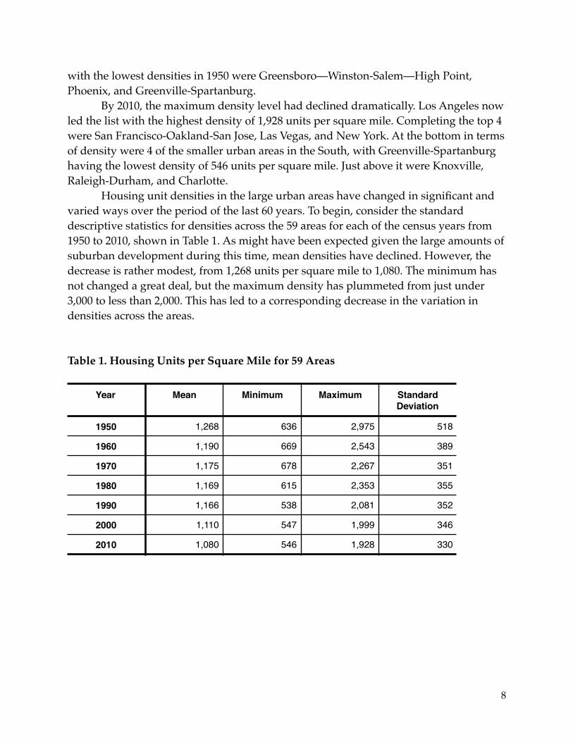
Housing unit densities in the large urban areas have changed in significant and varied ways over the period of the last 60 years. To begin, consider the standard descriptive statistics for densities across the 59 areas for each of the census years from 1950 to 2010, shown in Table 1. As might have been expected given the large amounts of suburban development during this time, mean densities have declined. However, the decrease is rather modest, from 1,268 units per square mile to 1,080. The minimum has not changed a great deal, but the maximum density has plummeted from just under 3,000 to less than 2,000. This has led to a corresponding decrease in the variation in densities across the areas.
Table 1. Housing Units per Square Mile for 59 Areas
Year Mean Minimum Maximum Standard Deviation
1950 1,268 636 2,975 518
1960 1,190 669 2,543 389
1970 1,175 678 2,267 351
1980 1,169 615 2,353 355
1990 1,166 538 2,081 352
2000 1,110 547 1,999 346
2010 1,080 546 1,928 330
!8
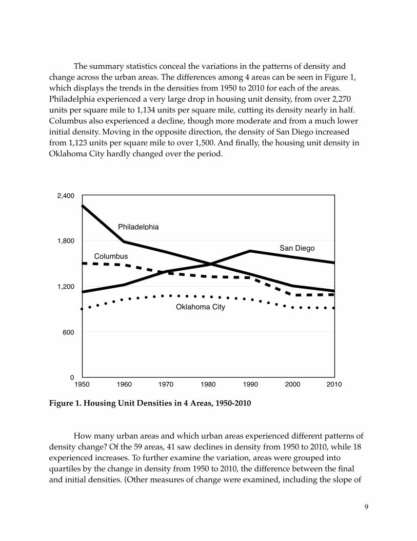
The summary statistics conceal the variations in the patterns of density and change across the urban areas. The differences among 4 areas can be seen in Figure 1, which displays the trends in the densities from 1950 to 2010 for each of the areas. Philadelphia experienced a very large drop in housing unit density, from over 2,270 units per square mile to 1,134 units per square mile, cutting its density nearly in half. Columbus also experienced a decline, though more moderate and from a much lower initial density. Moving in the opposite direction, the density of San Diego increased from 1,123 units per square mile to over 1,500. And finally, the housing unit density in Oklahoma City hardly changed over the period.
Figure 1. Housing Unit Densities in 4 Areas, 1950-2010
How many urban areas and which urban areas experienced different patterns of density change? Of the 59 areas, 41 saw declines in density from 1950 to 2010, while 18 experienced increases. To further examine the variation, areas were grouped into quartiles by the change in density from 1950 to 2010, the difference between the final and initial densities. (Other measures of change were examined, including the slope of
!9
0
600
1,200
1,800
2,400
1950 1960 1970 1980 1990 2000 2010
Philadelphia
Oklahoma City
ColumbusSan Diego
the trend lines for densities for each of the areas, and the results were very similar to those presented here using the simple change from the initial to the final density.) The density change quartiles are given along with the densities and density change for each area in the listing in Appendix B.
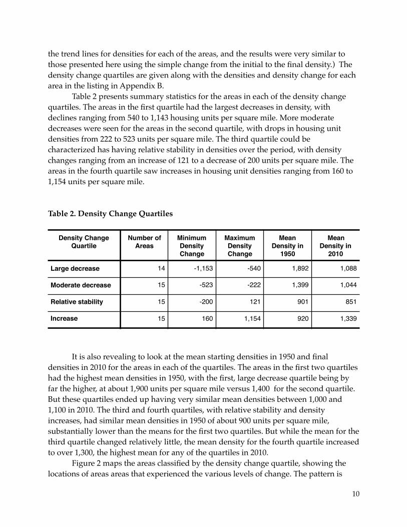
Table 2 presents summary statistics for the areas in each of the density change quartiles. The areas in the first quartile had the largest decreases in density, with declines ranging from 540 to 1,143 housing units per square mile. More moderate decreases were seen for the areas in the second quartile, with drops in housing unit densities from 222 to 523 units per square mile. The third quartile could be characterized has having relative stability in densities over the period, with density changes ranging from an increase of 121 to a decrease of 200 units per square mile. The areas in the fourth quartile saw increases in housing unit densities ranging from 160 to 1,154 units per square mile.
Table 2. Density Change Quartiles
It is also revealing to look at the mean starting densities in 1950 and final densities in 2010 for the areas in each of the quartiles. The areas in the first two quartiles had the highest mean densities in 1950, with the first, large decrease quartile being by far the higher, at about 1,900 units per square mile versus 1,400 for the second quartile. But these quartiles ended up having very similar mean densities between 1,000 and 1,100 in 2010. The third and fourth quartiles, with relative stability and density increases, had similar mean densities in 1950 of about 900 units per square mile, substantially lower than the means for the first two quartiles. But while the mean for the third quartile changed relatively little, the mean density for the fourth quartile increased to over 1,300, the highest mean for any of the quartiles in 2010.
Figure 2 maps the areas classified by the density change quartile, showing the locations of areas areas that experienced the various levels of change. The pattern is
Density Change Quartile
Number of Areas
Minimum Density Change
Maximum Density Change
Mean Density in
1950
Mean Density in
2010
Large decrease 14 -1,153 -540 1,892 1,088
Moderate decrease 15 -523 -222 1,399 1,044
Relative stability 15 -200 121 901 851
Increase 15 160 1,154 920 1,339
!10
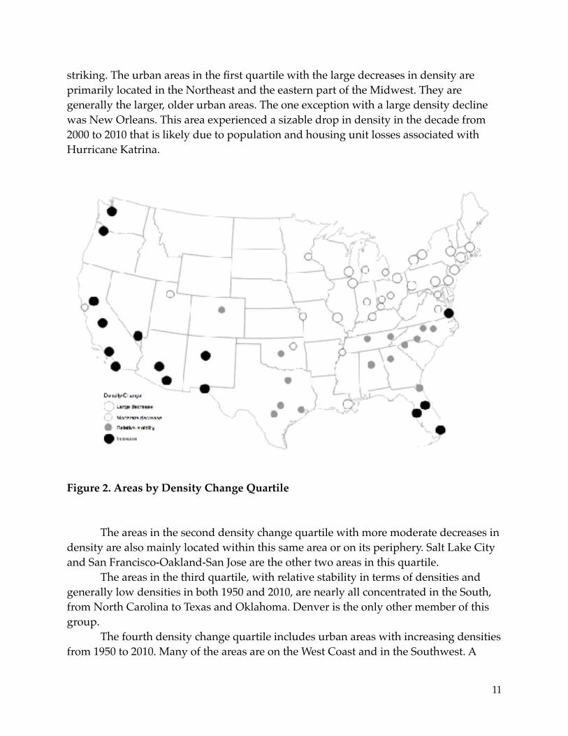
striking. The urban areas in the first quartile with the large decreases in density are primarily located in the Northeast and the eastern part of the Midwest. They are generally the larger, older urban areas. The one exception with a large density decline was New Orleans. This area experienced a sizable drop in density in the decade from 2000 to 2010 that is likely due to population and housing unit losses associated with Hurricane Katrina.
Figure 2. Areas by Density Change Quartile
The areas in the second density change quartile with more moderate decreases in density are also mainly located within this same area or on its periphery. Salt Lake City and San Francisco-Oakland-San Jose are the other two areas in this quartile.
The areas in the third quartile, with relative stability in terms of densities and generally low densities in both 1950 and 2010, are nearly all concentrated in the South, from North Carolina to Texas and Oklahoma. Denver is the only other member of this group.
The fourth density change quartile includes urban areas with increasing densities from 1950 to 2010. Many of the areas are on the West Coast and in the Southwest. A
!11
smaller cluster of three areas is in Florida. Norfolk-Virginia Beach is the additional member of this group.
Factors Associated with Density and Density Change
The wide variation and clear patterning of density and density change across the period raise the question of what factors might be associated with this variation. In this exploratory analysis, factors associated with density levels in 1950 and 2010 are considered first. Following is an examination of factors associated with the change in density over the period. In both cases, regression models are used to examine the association of possible predictors with density and density change.
Factors Associated with Density in 1950 and 2010
Basic economic theory and the standard monocentric model of urban structure suggest that the density of an urban area should be directly related to the size of the area. With greater numbers competing for space, land prices will be higher and densities greater (Muth 1969; Mills 1972). So the first factor to be considered as a predictor of density will be the number of housing units in the urban area. Examination of the scatterplots shows the relationships between housing units and density to be nonlinear. The log of the number of housing units is therefore used as the variable in the regression model.
Housing is a relatively permanent, long-lasting commodity. If housing built during one era tends to have higher or lower densities than housing built in another era, then the densities of urban area may depend upon the relative amounts of housing built during the various periods. The monocentric model predicts that densities will be directly related to transportation costs. In the periods before widespread use of the automobile, relative transportation costs (particularly time costs) would have been higher, leading to the greater densities seen in large cities in the late nineteenth century. Lower incomes among the newly arrived immigrants in this period would also be presumed to be associated with higher densities. Following this logic, Muth (1969: 192-193) used the age of housing as a predictor of densities within urban areas. Harrison and Kain (1974) used the age of housing as an alternative to the monocentric model for predicting density patterns within urban areas. The hypothesis here is that densities in urban areas will be related to the proportion of the area that was developed in an earlier period in which densities were generally higher. To estimate this, the size of the area at the earlier time as a percentage of its current size is used as the predictor in the model.
The data being used do not include information on the extent of the urban areas prior to 1950. In 1910, the Census for the first time attempted to capture the larger urban areas that extended beyond the major cities by defining Metropolitan Districts as
!12
aggregations of civil divisions. The populations of these Metropolitan Districts in 1910 are used to create the estimate of the amount of older development, which is then compared to the population of the Urbanized Areas in 1950. (Population had to be used rather than housing units since the census did not begin collecting data on housing until 1940. And the census Urbanized Areas had to be used because the census tract estimates of housing units used in defining the urban areas do not include populations for 1950). The variable used as the predictor of density in 1950 is the 1910 Metropolitan District population as a percentage of the 1950 Urbanized Area population (U.S. Bureau of the Census 1913: pp. 73-74 and Tables 50, 51, and 59; 1952: Tables 17 and 24; 1953, Table 32). For areas that were not designated as Metropolitan Districts or the related city plus adjacent area designation in 1910, the populations of the cities themselves were used. Since these were smaller cities with populations less than 100,000, the populations in surrounding suburban areas was likely rather small.
Now comes the issue of the choice of the analogous variable to be used as a predictor of density in 2010. One possibility is to assume that the amount of development before the widespread use of the automobile should again be the focus, suggesting the use of the 1910 population for the Metropolitan Districts as a percentage of the 2010 population for the urban area. Alternatively, the variable for 1950 density is the 1910 population, 40 years earlier, as the percentage of the 1950 population. So the second possibility would be to use the 1970 population as a percentage of the (40 years later) 2010 population. Initial models were estimated using each of these variables as the predictor.
A third factor that may affect the density of urban areas is the presence of physical restrictions on the expansion of the urban area. Such restrictions would decrease the supply of land available for development in convenient locations, increasing the price land and the density of development. Two types of physical restrictions are considered here—the presence of mountains or of wetlands that block urban expansion. Burchfield, et al. (2006) found the presence of high mountains reduced urban sprawl measured as the fragmentation of developed areas, but they did not address density. Bereitschaft and Debbage (2014) likewise suggested the importance of barriers such as mountains and wetlands for the fragmentation of development. Paulsen (2014) includes steeply sloped land and wetlands in models predicting change in density, among other measures of sprawl.
For this research, areas are considered to be restricted if significant portions of the 2010 urban area were adjacent to areas of mountains or wetlands having little or no development. This judgment was subjective. As a check, more generous designations 4
The areas considered restricted by mountains are Albuquerque, Denver, El Paso, Las Vegas, Los 4
Angeles, Phoenix, Salt Lake City-Ogden-Provo, San Diego, San Francisco-Oakland-San Jose, and Tucson. The areas restricted by wetlands are Miami-Fort Lauderdale-West Palm Beach and New Orleans.
!13
were tried where less of the urban area was adjacent to these features or where the restricting areas tended to be near rather than adjacent to the current urban area. The alternative measures produced similar though not quite as strong results in the model. The predictor is a dummy variable indicating the presence of the restrictions.
Obviously other features such as large bodies of water and even large rivers would be barriers to urban expansion. Measures of these were considered. However, the location of urban areas on water is strongly related to the size and age of urban areas, as initial urban settlement occurred in such locations because of the importance of water for transportation. These measures were not significant in models in which the size and age of urban areas were included, so they are not used in the models reported.
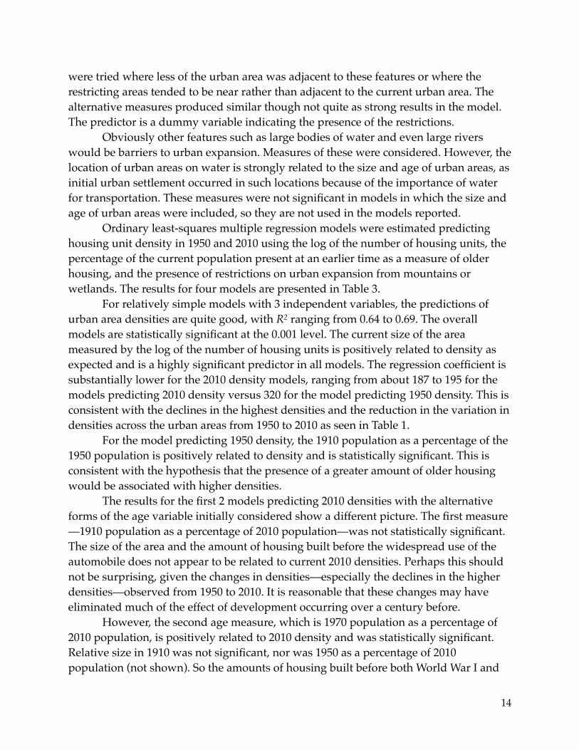
Ordinary least-squares multiple regression models were estimated predicting housing unit density in 1950 and 2010 using the log of the number of housing units, the percentage of the current population present at an earlier time as a measure of older housing, and the presence of restrictions on urban expansion from mountains or wetlands. The results for four models are presented in Table 3.
For relatively simple models with 3 independent variables, the predictions of urban area densities are quite good, with R2 ranging from 0.64 to 0.69. The overall models are statistically significant at the 0.001 level. The current size of the area measured by the log of the number of housing units is positively related to density as expected and is a highly significant predictor in all models. The regression coefficient is substantially lower for the 2010 density models, ranging from about 187 to 195 for the models predicting 2010 density versus 320 for the model predicting 1950 density. This is consistent with the declines in the highest densities and the reduction in the variation in densities across the urban areas from 1950 to 2010 as seen in Table 1.
For the model predicting 1950 density, the 1910 population as a percentage of the 1950 population is positively related to density and is statistically significant. This is consistent with the hypothesis that the presence of a greater amount of older housing would be associated with higher densities.
The results for the first 2 models predicting 2010 densities with the alternative forms of the age variable initially considered show a different picture. The first measure—1910 population as a percentage of 2010 population—was not statistically significant. The size of the area and the amount of housing built before the widespread use of the automobile does not appear to be related to current 2010 densities. Perhaps this should not be surprising, given the changes in densities—especially the declines in the higher densities—observed from 1950 to 2010. It is reasonable that these changes may have eliminated much of the effect of development occurring over a century before.
However, the second age measure, which is 1970 population as a percentage of 2010 population, is positively related to 2010 density and was statistically significant. Relative size in 1910 was not significant, nor was 1950 as a percentage of 2010 population (not shown). So the amounts of housing built before both World War I and
!14
before 1950 were not significantly related to current densities, but the total amount built before 1970 was. However there is little to suggest dramatic changes in development patterns occurred around 1970 that would have affected density levels.
Table 3. Regression: Factors Associated with Density
Moving in the other direction and looking at more recent years, using 1980, 1990, and 2000 populations as percentages of 2010 population, the strength of the relationship to density tends to increase over time, with the regression coefficient increasing from 3.21 from 1970 population to 7.53 for 2000 population as a percent of 2010 population. (Results for the latter are shown in the fourth column of Table 3.) This suggests that for
Independent Variable Dependent Variable
Housing Unit Density in
1950
Housing Unit Density in 2010
Log of current housing units 1950/2010
307.70 ** 194.71 ** 187.34 ** 193.17 **
(36.61) (30.67) (28.93) (28.65)
1910 population as percent of 1950 population
6.64 * — — —
(2.26)
1910 population as percent of 2010 population
— 1.43 — —
(1.73)
1970 population as percent of 2010 population
— — 3.21 * —
(1.13)
2000 population as percent of 2010 population
— — — 7.53 *
(2.53)
Mountains or wetlands restricting urban expansion
186.91 459.61 ** 476.98 ** 429.91 **
(104.93) (69.08) (63.15) (61.77)
Constant -2,574.80 ** -1,655.42 ** -1,706.56 ** -2,263.07 **
(401.7) (413.32) (387.89) (440.4)
R2 0.680 ** 0.644 ** 0.685 ** 0.689 **
*Significant at the 0.01 level
**Significant at the 0.001 level
!15
predicting density in 2010, at least, the variable should perhaps be considered to be a measure of the amount of new development: The greater the amount of new development in the recent past, the lower the density.
With new development, some of that development occurs in formerly rural tracts that then become incorporated into the urban area as the density of the tract exceeds the minimum threshold. But development in a tract can take place over an extended period of time. Not all of the land within a tract will necessarily have been developed at the time of the first (or even second) census after the tract becomes urban (see, e.g., Ewing 2008). Therefore even if the density of residential development within newly developed subdivisions were as great or greater than the rest of the urban area, the overall density of the tract could be lower—potentially much lower—because of the presence of currently undeveloped land. And this can change in subsequent years as further development occurs in the area, filling in the vacant areas. Urban areas experiencing higher levels of new development might thus be expected to have lower overall densities due to the inclusion of more tracts that are partially developed.
The final predictor included in the models was the presence of physical restrictions on development by mountains or wetlands. This variable was not significant for the prediction of 1950 density. For all of the models predicting 2010 density, the variable had a positive and highly statistically significant relationship to density. The effect was substantial, with housing unit densities over 400 units per square mile greater in the areas having the restrictions, compared to the mean of slightly under 1,100 units per square miles for all urban areas in 2010.
Factors Associated with Density Change from 1950 to 2010
The dramatic decline in maximum densities from 1950 to 2010 and the convergence of densities across the urban areas indicate that the change in density is necessarily inversely related to the initial density in 1950. Only areas with the higher starting densities could have experienced declines of the magnitudes observed across this period. So initial density is one factor to be considered in the prediction of density change.
For the prediction of density levels, the argument was made and the results showed that densities were related to the size of the urban area. It therefore follows that the change in density should be related to the change in the size of the area, measured here as the difference in the number of housing units between 1950 and 2010.
The physical restrictions on urban expansion resulting from the presence of mountains or wetlands were significantly related to 2010 density but not to the density in 1950. It is therefore reasonable to expect that these restrictions would be related to the change in density.
!16
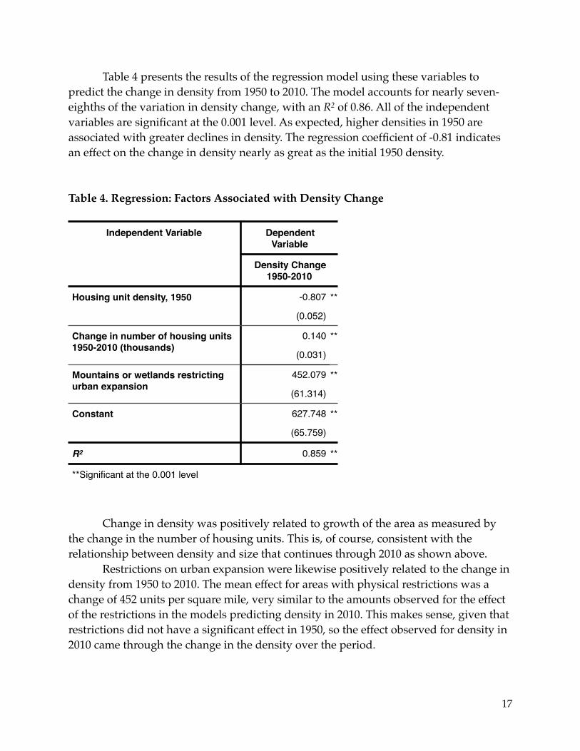
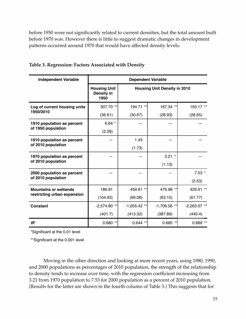
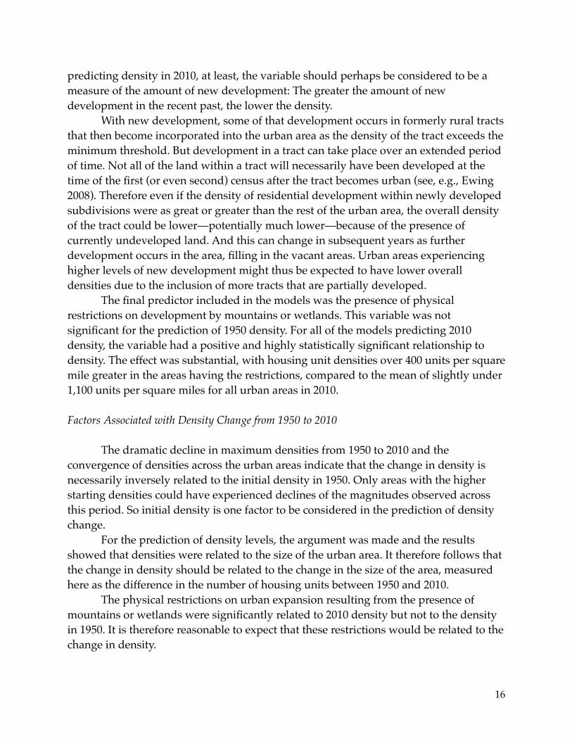
Table 4 presents the results of the regression model using these variables to predict the change in density from 1950 to 2010. The model accounts for nearly seven-eighths of the variation in density change, with an R2 of 0.86. All of the independent variables are significant at the 0.001 level. As expected, higher densities in 1950 are associated with greater declines in density. The regression coefficient of -0.81 indicates an effect on the change in density nearly as great as the initial 1950 density.
Table 4. Regression: Factors Associated with Density Change
Change in density was positively related to growth of the area as measured by the change in the number of housing units. This is, of course, consistent with the relationship between density and size that continues through 2010 as shown above.
Restrictions on urban expansion were likewise positively related to the change in density from 1950 to 2010. The mean effect for areas with physical restrictions was a change of 452 units per square mile, very similar to the amounts observed for the effect of the restrictions in the models predicting density in 2010. This makes sense, given that restrictions did not have a significant effect in 1950, so the effect observed for density in 2010 came through the change in the density over the period.
Independent Variable Dependent Variable
Density Change 1950-2010
Housing unit density, 1950 -0.807 **
(0.052)
Change in number of housing units 1950-2010 (thousands)
0.140 **
(0.031)
Mountains or wetlands restricting urban expansion
452.079 **
(61.314)
Constant 627.748 **
(65.759)
R2 0.859 **
**Significant at the 0.001 level
!17
Conclusion
The housing unit densities of urban areas vary widely, as do the changes in densities over the period from 1950 to 2010. These differences varied by region of the country. Those urban areas that started with the highest densities and experienced the greatest declines were located mainly in and near the Northeast and Midwest. Areas with lower densities that showed relatively lower changes in density were concentrated in the South. Urban areas along the Pacific Coast, in the Southwest, and in Florida saw increases in densities, with some emerging as the highest-density urban areas by 2010.
Urban area densities are associated with the sizes of the urban areas, and changes in density were associated with changes in the numbers of housing units. Urban areas that were larger in 1910 had higher densities in 1950. This effect of greater amounts of older housing seems to have disappeared by 2010. The presence of barriers to urban expansion in the form of mountains or wetlands was associated with greater increases in density and higher densities in 2010, but not in 1950.
These results show that the commonly held view that the densities of urban areas in the modern era are inevitably declining is just not true. Many urban areas, a majority of large urban areas in the United States, have experienced decreases in densities since the mid-twentieth century. But densities were stable or increased for many other areas. It is important to recognize these as significant alternate trajectories of urban change. When increased urban densities are observed, they should not be dismissed as outliers, as exceptional cases to be attributed to unique and unusual circumstances.
The older large cities of the Northeast and Midwest have long been viewed as the prototypical American cities, though the early growth of Los Angeles emphasized that very different types of urban areas were possible. The clear pattern of regional differences shows how the single measure of urban density (and its change) can identify distinctive types of urban areas.
The findings suggest numbers of questions for further research. The importance of recent growth for predicting urban area density in 2010 raises the issue of the temporal patterns of development at the urban fringe. It is too easy to view urban area expansion as development at the fringe that occurs during the decade in which an area changes from rural to urban. In reality, the development of new urban areas likely occurs over much longer periods of time both before and after that period after which the area becomes designated as part of the urban area. Understanding these development patterns will contribute to our knowledge of urban expansion.
The presence of barriers to urban expansion was found to be associated with increased urban area densities. The nature and details of these effects can be explored in more detail. It is important to understand how densities within the urban areas are increased in the face of such pressures. The effects of such barriers and pressures on urban development in the larger regions of which those urban areas are a part can also
!18
be explored. For example, is some development shifted to other areas in those regions beyond the barriers?
This study has focused on the densities of urban areas—those areas with densities reaching a threshold for designation as urban. It has not addressed levels of development in the broader outlying exurban areas, related to the urban areas but beyond the contiguous built-up territory. A few studies have examined exurban areas, most at a single point in time. Berube, et al. (2006) provide one of the more comprehensive studies and review earlier work. Theobald (2001) did classify areas having exurban densities for numbers of years, but the results are limited to national totals and maps, with no consideration of the exurban areas surrounding individual urban areas.
Finally, this study has been limited to the consideration of the overall densities of urban areas. How the distribution of housing units and their densities varies within those urban areas is an obvious next question. Studies of negative exponential density gradients have looked at changes in those patterns over time. However, with often increasing decentralization and decreasing density gradients, such studies may be capturing less and less of the relevant variation in development within urban areas. A number of studies have attempted more comprehensive measurement of urban patterns within the context of studying multiple dimensions of urban sprawl, but these have examined the patterns at only 1 or 2 points in time (e.g., Galster, et al. 2001; Ewing, Pendall, and Chen 2002). Understanding how the distribution of housing units and their densities have changed within urban areas over an extended period of time would further contribute to understanding of how urban areas grow and change.
References
Anas, Alex, Richard Arnott, and Kenneth A. Small. 1998. Urban spatial structure. Journal of Economic Literature 36, 1 (September): 1426-1464.
Angel, Shlomo. 2012. Planet of Cities. Cambridge, MA: Lincoln Institute of Land Policy.Angel, Shlomo, Alejandro Blei, Jason Parent, and Daniel A. Civco. 2011. The decline in transit-
sustaining densities in U.S. cities, 1910– 2000. In Climate Change and Land Policies, Gregory K. Ingram and Yu-Hung Hong, eds. Cambridge, MA: Lincoln Institute of Land Policy, pp. 191-212.
Bereitschaft, Bradley, and Keith Debbage. 2014. Regional variations in urban fragmentation among U.S. metropolitan and megapolitan areas. Applied Spatial Analysis and Policy 7, 2 (June): 119-146.
Berube, Alan, Audrey Singer, Jill H. Wilson, and William H. Frey. 2006. Finding Exurbia: America’s Fast-Growing Communities at the Urban Fringe. Washington, DC: The Brookings Institution.
Bruegmann, Robert. 2005. Sprawl: A Compact History. Chicago: University of Chicago Press.
!19
Burchfield, Marcy, Henry C. Overman, Diego Puga, and Matthew A. Turner. 2006. Causes of sprawl: A portrait from space. The Quarterly Journal of Economics 121, 2 (May): 587-633.
Clark, Colin. 1951. Urban population densities. Journal of the Royal Statistical Society, Series A 114, 4: 490-496.
Clark, T. A. 2013. Metropolitan density, energy efficiency, and carbon emissions: Multi-attribute tradeoffs and their policy implications. Energy Policy 53 (February): 413-428.
Cutsinger, Jackie, George Galster, Harold Wolman, Royce Hanson, and Douglas Towns. 2005. Verifying the multi-dimensional nature of metropolitan land use: Advancing the understanding and measurement of sprawl. Journal of Urban Affairs 27, 3 (August): 235-259.
Ewing, Reid. 1997. Is Los Angeles-style sprawl desirable? Journal of the American Planning Association 63, 1 (Winter): 197-126.
Ewing, Reid. 2008. Characteristics, causes, and effects of sprawl: A literature review. In Urban Ecology: An International Perspective on the Interaction Between Humans and Nature, ed. John M. Marzluff, Eric Shulenberger, Wilfried Endlicher, Marina Alberti, Gordon Bradley, Clare Ryan, Ute Simon, Craig ZumBrunnen. New York: Springer, pp. 519-535.
Ewing, Reid, and Robert Cervero. 2010. Travel and the built environment: A meta-analysis. Journal of the American Planning Association 76, 3 (Summer): 265-294.
Ewing, Reid, and Shima Himidi. 2014. Measuring Urban Sprawl and Validating Sprawl Measures. Prepared for National Cancer Institute, National Institutes of Health; Ford Foundation; Smart Growth America. Metropolitan Research Center, University of Utah. Downloaded from http://gis.cancer.gov/tools/urban-sprawl/ on April 8, 2014.
Ewing, Reid, Rolf Pendall, and Don Chen. 2002. Measuring Sprawl and Its Impact. Volume I. Washington, DC: Smart Growth America. Downloaded from http://www.smartgrowthamerica.org/documents/MeasuringSprawlTechnical.pdf on April 8, 2014.
Fulton, William, Rolf Pendall, Mai Nguyen, and Alice Henderson. 2001. Who Sprawls Most? Washington, DC: Brookings Institution.
Galster, George, Royce Hanson, Machael R. Ratcliff, Harold Wolman, Stephen Coleman, and Jason Freihage. 2001. Wrestling sprawl to the ground: Defining and measuring an elusive concept. Housing Policy Debate 12, 4: 681-717.
Glaeser, Edward L., and Matthew E. Kahn. 2004. Sprawl and urban growth. Handbook of Regional and Urban Economics 4: 2481-2527.
Grazi, Fabio, Jeroen C. J. M. van den Bergh, and Jos. N. van Ommeren. 2008. An empirical analysis of urban form, transport, and global warming. The Energy Journal 29, 4 (March): 97-122.
Guerra, Erick, and Robert Cervero. 2011. Cost of a ride: The effects of densities on fixed-guideway transit ridership and costs. Journal of the American Planning Association 77, 3 (Summer): 267-290.
Guest, Avery M. 1975. Population suburbanization in American metropolitan areas, 1940-1970. Geographical Analysis 7 (July): 267-283.
Hammer, Roger B., Susan I. Stewart, Richelle L. Winkler, Volker C. Radeloff, and Paul R. Voss. 2004. Characterizing dynamic spatial and temporal residential density patterns from 1940-1990 across the North Central United States. Landscape and Urban Planning 69, 2-3: 183-199.
!20
Harrison, David, Jr., and John F. Kain. 1974. Cumulative urban growth and urban density functions. Journal of Urban Economics 1, 1 (January): 61-98.
Harvey, Robert. O. and W. A. V. Clark. 1965. The nature and economics of urban sprawl. Land Economics 41, 1 (February): 1-9.
Laidley, Thomas. 2015. Measuring sprawl: A new index, recent trends, and future research. Urban Affairs Review (forthcoming).
Lopez, Russ, and H. Patricia Hynes. 2003. Sprawl in the 1990s: Measurement, distribution, and trends. Urban Affairs Review 38, 3 (January): 325-355.
Malpezzi, Stephen, and Wen-Kai Guo. 2001. Measuring “sprawl:” Alternative measures of form in U.S. metropolitan areas. Center for Urban Land Economics Research, University of Wisconsin, Madison. Downloaded from http://smalpezzi.marginalq.com/documents/Alternative%20Measures%20of%20Urban%20Form.doc on April 7, 2014.
Mills. Edwin S. 1972. Studies in the Structure of the Urban Economy. Baltimore: Johns Hopkins Press for Resources for the Future.
Muth, Richard F. 1969. Cities and Housing: The Spatial Pattern of Urban Residential Land Use. Chicago: University of Chicago Press.
Nasser, Haya El and Paul Overberg. 2001. A comprehensive look at sprawl in America. USA Today, February 22. Downloaded from http://usatoday30.usatoday.com/news/sprawl/main.htm on April 9, 2014.
Newman, Peter W. G. and Jeffrey R. Kenworthy. 1989. Gasoline consumption and cities: A comparison of U.S. cities with a global survey. Journal of the American Planning Association 55, 1 (Winter): 24-37.
Paulsen, K. 2014. Geography, policy or market? New evidence on the measurement and causes of sprawl (and infill) in US metropolitan regions. Urban Studies 41, 12 (September): 2629-2645.
Pendall, R. 1999. Do land-use controls cause sprawl? Environment & Planning B 26, 5: 555-571.Radeloff, Volker C., Roger B. Hammer, Paul R. Voss, Alice E. Hagen, Donald R. Field, and David
J. Mladenoff. 2001. Human demographic trends and landscape level forest management in the northwest Wisconsin Pine Barrens. Forest Science 47, 2 (May): 229-241.
Radeloff, Volker C., Roger B. Hammer, and Susan L. Stewart. 2005. Rural and suburban sprawl in the U.S. midwest from 1940 to 2000 and its relation to forest fragmentation. Conservation Biology 19, 3 (June): 793-805.
Stone, Brian, Adam C. Mednick, Tracey Holloway, and Scott N. Spak. 2007. Is compact growth good for air quality? Journal of the American Planning Association 73, 4 (Autumn): 404-418.
Su, Qing. 2011. The effects of population density, road network density, and congestion on household gasoline consumption in U.S. urban areas. Energy Economics 33, 3 (May): 445-452.
Taylor, Brian D., Douglas Miller, Hiroyuki Iseki, and Camile Fink. 2009. Nature and/or nurture: Analyzing the determinants of transit ridership across US urban areas. Transportation Research Part A 43, 1 (January): 60-77.
Theobald, David M. 2001. Land-use dynamics beyond the urban fringe. Geographical Review 91, 3 (July): 544-564.
U.S. Bureau of the Census. 1913. Thirteenth Census of the United States Taken in the Year 1910. Vol. 1. Population 1910. General Report and Analysis. Washington DC: Government Printing Office.
!21
U.S. Bureau of the Census. 1952. U.S. Census of Population: 1950. Vol. I, Number of Inhabitants. United States Summary. Washington, DC: U.S. Government Printing Office.
U.S. Bureau of the Census. 1953. U.S. Census of Housing: 1950. Vol. 1, General Characteristics. Part 1. U.S. Summary. Washington, DC: U.S. Government Printing Office.
U.S. Bureau of the Census. 2002. Urban area criteria for the 2000 Census. Federal Register 67, 51 (Friday, March 15): 11663-11670.
U.S. Bureau of the Census. 2011. Urban area criteria fot the 2010 Census. Federal Register 76, 164 (Wednesday, August 24): 53030-53043.
U.S. Bureau of the Census. 2012. Census block shapefiles with 2010 Census population and housing unit counts. Downloaded from http://www.census.gov/geo/www/tiger/tgrshp2010/pophu.html on September 29, 2012.
U.S. Bureau of the Census. 2013. Core based statistical areas (CBSAs) and combined statistical areas (CSAs) 2013 delineation file. February 2013. Downloaded from https://www.census.gov/population/metro/data/def.html on February 13, 2014.
U.S. National Atlas. 2014. Airports shapefile. Downloaded from http://www.nationalatlas.gov/atlasftp.html?openChapters=chptrans#chptrans on April 4, 2014.
U.S. Office of Management and Budget. 2010. 2010 Standards for delineating Metropolitan and Micropolitan Statistical Areas. Federal Register 75, 128 (June 28, 2010): 37246-37252.
Urban Institute and Geolytics. 2003. Census CD Neighborhood Change Database (NCDB): 1970-2000 Tract Data. Somerville, NJ: Geolytics, Inc.
Wirth, Louis. 1938. Urbanism as a way of life. American Journal of Sociology 44, 1 (July): 1-24.Zhao, Zhenxiang, and Robert Kaestner. 2010. Effects of urban sprawl on obesity. Journal of Health
Economics 29, 6 (December): 779-87.
Appendix A. Urban Area Delineation
The procedures used for defining the urban areas here generally follows those used by the Census for the 2010 Urbanized Areas (U.S. Bureau of the Census 2011) with modifications to reflect the use of census tracts only and not block data.
Tracts are included in the urban area that have a minimum density of 213.33 housing units per square mile, are edge-contiguous with the main urban area, and are within the CSA or MSA boundary. Contiguity is established if a common border can be seen at a scale of 1:100,000.
Urban tracts separated by water or by tracts below the density cutoff along major rivers are considered to be contiguous. The tracts along rivers are included in the urban area if the majority of their boundaries on both sides of the river are adjacent to urban tracts.
A nonurban area of less than 5 square miles surrounded by the urban area or by a major body of water and urban tracts is considered to be part of the urban area. A small number of larger surrounded nonurban areas were also considered to be urban if current satellite imagry showed the area to be virtually completely developed (these were large industrial areas).
!22
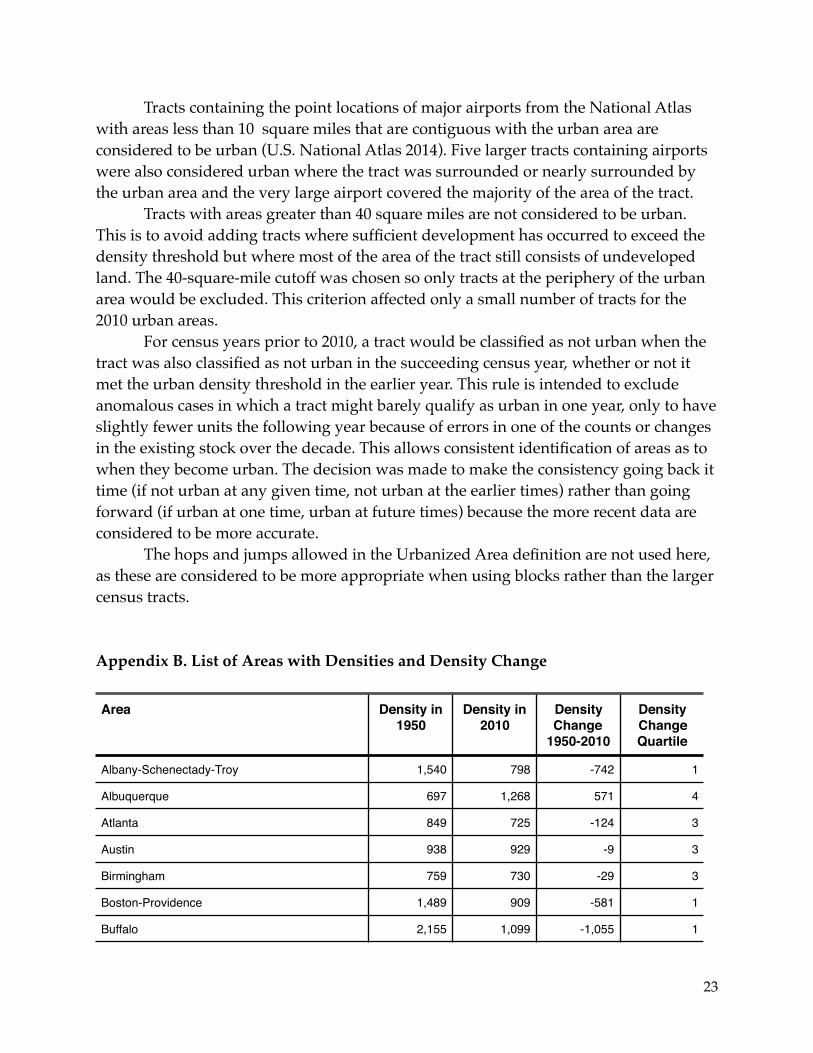
Tracts containing the point locations of major airports from the National Atlas with areas less than 10 square miles that are contiguous with the urban area are considered to be urban (U.S. National Atlas 2014). Five larger tracts containing airports were also considered urban where the tract was surrounded or nearly surrounded by the urban area and the very large airport covered the majority of the area of the tract.
Tracts with areas greater than 40 square miles are not considered to be urban. This is to avoid adding tracts where sufficient development has occurred to exceed the density threshold but where most of the area of the tract still consists of undeveloped land. The 40-square-mile cutoff was chosen so only tracts at the periphery of the urban area would be excluded. This criterion affected only a small number of tracts for the 2010 urban areas.
For census years prior to 2010, a tract would be classified as not urban when the tract was also classified as not urban in the succeeding census year, whether or not it met the urban density threshold in the earlier year. This rule is intended to exclude anomalous cases in which a tract might barely qualify as urban in one year, only to have slightly fewer units the following year because of errors in one of the counts or changes in the existing stock over the decade. This allows consistent identification of areas as to when they become urban. The decision was made to make the consistency going back it time (if not urban at any given time, not urban at the earlier times) rather than going forward (if urban at one time, urban at future times) because the more recent data are considered to be more accurate.
The hops and jumps allowed in the Urbanized Area definition are not used here, as these are considered to be more appropriate when using blocks rather than the larger census tracts.
Appendix B. List of Areas with Densities and Density Change
Area Density in 1950
Density in 2010
Density Change
1950-2010
Density Change Quartile
Albany-Schenectady-Troy 1,540 798 -742 1
Albuquerque 697 1,268 571 4
Atlanta 849 725 -124 3
Austin 938 929 -9 3
Birmingham 759 730 -29 3
Boston-Providence 1,489 909 -581 1
Buffalo 2,155 1,099 -1,055 1
!23
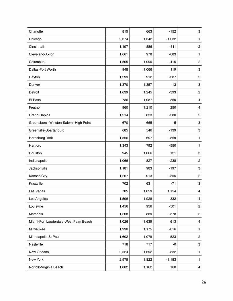
Charlotte 815 663 -152 3
Chicago 2,374 1,342 -1,032 1
Cincinnati 1,197 886 -311 2
Cleveland-Akron 1,661 978 -683 1
Columbus 1,505 1,090 -415 2
Dallas-Fort Worth 948 1,066 119 3
Dayton 1,299 912 -387 2
Denver 1,370 1,357 -13 3
Detroit 1,639 1,245 -393 2
El Paso 736 1,087 350 4
Fresno 960 1,210 250 4
Grand Rapids 1,214 833 -380 2
Greensboro--Winston-Salem--High Point 670 665 -5 3
Greenville-Spartanburg 685 546 -139 3
Harrisburg-York 1,556 697 -859 1
Hartford 1,343 792 -550 1
Houston 945 1,066 121 3
Indianapolis 1,066 827 -238 2
Jacksonville 1,181 983 -197 3
Kansas City 1,267 913 -355 2
Knoxville 702 631 -71 3
Las Vegas 705 1,859 1,154 4
Los Angeles 1,596 1,928 332 4
Louisville 1,456 956 -501 2
Memphis 1,268 889 -378 2
Miami-Fort Lauderdale-West Palm Beach 1,026 1,639 613 4
Milwaukee 1,990 1,175 -816 1
Minneapolis-St Paul 1,602 1,079 -523 2
Nashville 718 717 -0 3
New Orleans 2,524 1,692 -832 1
New York 2,975 1,822 -1,153 1
Norfolk-Virginia Beach 1,002 1,162 160 4
!24
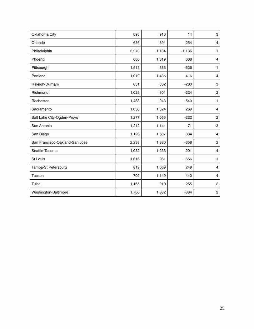
Oklahoma City 898 913 14 3
Orlando 636 891 254 4
Philadelphia 2,270 1,134 -1,136 1
Phoenix 680 1,319 638 4
Pittsburgh 1,513 886 -626 1
Portland 1,019 1,435 416 4
Raleigh-Durham 831 632 -200 3
Richmond 1,025 801 -224 2
Rochester 1,483 943 -540 1
Sacramento 1,056 1,324 269 4
Salt Lake City-Ogden-Provo 1,277 1,055 -222 2
San Antonio 1,212 1,141 -71 3
San Diego 1,123 1,507 384 4
San Francisco-Oakland-San Jose 2,238 1,880 -358 2
Seattle-Tacoma 1,032 1,233 201 4
St Louis 1,616 961 -656 1
Tampa-St Petersburg 819 1,069 249 4
Tucson 709 1,149 440 4
Tulsa 1,165 910 -255 2
Washington-Baltimore 1,766 1,382 -384 2
!25