Embed Size (px)
Citation preview
Density Functional Studies
on EPR Parameters and Spin-Density Distributions
of Transition Metal Complexes
DISSERTATION
ZUR ERLANGUNG DES NATURWISSENSCHAFTLICHEN DOKTORGRADES
DER BAYERISCHEN JULIUS-MAXIMILIANS-UNIVERSITÄT WÜRZBURG
VORGELEGT VON
CHRISTIAN REMENYI
AUS NECKARSULM
WÜRZBURG 2006
Eingereicht am: ___________________________________
bei der Fakultät für Chemie und Pharmazie
Gutachter: ___________________________________
Gutachter: ___________________________________
der Dissertation
Prüfer: ___________________________________
Prüfer: ___________________________________
Prüfer: ___________________________________
des Öffentlichen Promotionskolloquiums
Tag des Öffentlichen Promotionskolloquiums: __________
Doktorurkunde ausgehändigt am: ____________________

i
Contents
Introduction 1
Background and Motivation 1
Objectives of the Study 3
Acknowledgements 5
Chapter 1: Density Functional Theory 7
1.1. Density Functional Theory: Relevance and History 7
1.2. The Fundamentals:
Elementary Quantum Chemistry and the Hartree-Fock Approximation 7
1.2.1. The Schrödinger Equation 7
1.2.2. The Hartree-Fock Method 8
1.3. Density Functional Theory – The Principles 10
1.3.1. The Hohenberg-Kohn Theorems 10
1.3.2. The Kohn-Sham Approach 11
1.4. Density Functional Theory – The Machinery 12
1.4.1. Functionals 12
1.4.2. The LCAO Approach 14
1.4.3. Basis Sets and Pseudopotentials 15
Chapter 2: Electron Paramagnetic Resonance 17
2.1. The Electron Spin 17
2.1.1. Where does it come from? – The Electron Spin as a Theoretical Concept 17
2.1.2. The Effective Spin Hamiltonian 18
2.1.3. Measuring the Electronic Spin 19
2.2. From an Effective Spin Hamiltonian to a Quantum Mechanical One 20
2.2.1. The Breit-Pauli Hamiltonian 20
2.2.2. Operators Relevant for the Electron-Zeeman and the Hyperfine Interaction 22
2.3. Calculation of g- and A-Tensors: Perturbation Theory 25
2.3.2. Perturbation Theory Expressions for the Electronic g-Tensor 27
2.3.3. Perturbation Theory Expressions for the A-Tensor 28
2.4. SO Operators and the Gauge Origin of the g-Tensor 29
2.5. More than one Spin Center: Exchange Interaction 29
2.5.1. The Heisenberg-Dirac-van-Vleck Hamiltonian 29
CONTENTS
ii
2.5.2. The Broken-Symmetry Approach for Calculating J Values 30
Chapter 3: Spin-Orbit Corrections to Hyperfine Coupling Constants 33
3.1. Introduction 33
3.2. Computational Details 34
3.3. Results and Discussion 34
3.3.1. Carbonyl Complexes: Comparison to Semiempirical SO Corrections 34
3.3.2. Copper Complexes 36
3.3.3. Manganese Complexes 41
3.3.4. Use of SO-ECPs on Heavy Atoms 41
3.4. Conclusions 44
Chapter 4: Amavadin as a Test Case for the Calculation of EPR Parameters 45
4.1. Introduction 45
4.2. Computational Details 46
4.3. Results and Discussion 46
4.3.1. g-Tensor 47
4.3.2. A-Tensor in the First-Order Approximation 48
4.3.3. Second-Order SO Corrections to the A-Tensor. 49
4.3.4. Orientation of the Tensors 50
4.3.5. Understanding the Effect of Exchange-Correlation Functional
on Bonding and EPR Parameters 51
4.4. Conclusions 54
Chapter 5: EPR Parameters and Spin-Density Distributions of Azurin
and other Blue-Copper Proteins 57
5.1. Introduction 57
5.2. Computational Details 59
5.3. Results and Discussion 60
5.3.1. Spin-density Distribution 60
5.3.2. Relevance of the Axial Ligands in Azurin for Spin-Density Distribution 63
5.3.3. The g-Tensor of Azurin 64
5.3.4. 65Cu Hyperfine Coupling Constants 67
5.3.5. Histidine Nitrogen Hyperfine Coupling Constants 73
5.3.6. Tensor Orientations 74
5.3.7. The EPR Parameters of a Selenocysteine-Substituted Azurin 74
5.4. Conclusions 76
CONTENTS
iii
Chapter 6: Where is the Spin? Understanding Electronic Structure and g-Tensors
for Ruthenium Complexes with Redox-Active Quinonoid Ligands 79
6.1. Introduction 79
6.2. Computational Details 82
6.3. Results and Discussion 83
6.3.1. Molecular Structures 83
6.3.2. Spin Density Analyses 85
6.3.3. NPA Charges, Improved Assignments of Formal Oxidation States 90
6.3.4. g-Tensor Values and Orientations 93
6.3.5. Analysis of g-Tensors 99
6.3.6. The Origin of Spin Contamination. A Closer Look at the Bonding Situation 107
6.4. Conclusions 111
Chapter 7: EPR Paramaters and Spin-Density Distributions of Dicopper(I) Complexes
with bridging Azo and Tetrazine Radical Anion Ligands 113
7.1. Introduction 113
7.2. Computational Details 115
7.3. Results and Discussion 116
7.3.1. Structures 116
7.3.2. Spin-Density Distribution 117
7.3.3. Metal Hyperfine Coupling Tensors; Comparison with Experiment 120
7.3.4. Metal Hyperfine Couplings; Orbital Analysis 122
7.3.5. Ligand Hyperfine Couplings 125
7.3.6. g-Tensors: Comparison with Experiment and Dependence on Functional 129
7.3.7. Effect of the Phosphine Co-Ligands, Comparison of L = PH3 and L = PPh3. 133
7.3.8. Molecular-Orbital and Atomic Spin-Orbit Analyses of g-Tensors 135
7.4. Conclusions 137
Chapter 8: Bis(semiquinonato)copper Complexes – Change of Spin State
by Twisting the Ring System 139
8.1. Introduction 139
8.2. Computational Details 140
8.3. Results and Discussion 141
8.3.1. The g-Tensor as a Probe of the Electronic Structure 141
8.3.2. Spin-Density Distribution 144
CONTENTS
iv
8.3.3. The Change of Spin State: Geometrical or Electronic Effect? 145
8.3.4. Other Q-Cu-Q Systems 147
8.3.5. Exchange Coupling 148
8.4. Conclusions 149
Bibliography 151
Summary 161
Zusammenfassung 165
Curriculum Vitae 169
List of Publications 170
1
Introduction
Background and Motivation
In the awareness of many chemists Electron
Paramagnetic Resonance (EPR) spectroscopy
leads a shadowy existence. In contrast to Nuclear
magnetic resonance (NMR) spectroscopy, which
is today one of the standard tools for the struc-
ture determination especially for organic com-
pounds, EPR is regarded mostly as an exotic
technique limited to very special cases such as
paramagnetic organotransition metals and coor-
dination complexes or some curious organic
radicals. However, modern sciences have more
and more focused on the understanding of the
underlying principles of how life in general
works. Surprisingly, compounds which belong to
the branch of chemistry, which is named the
inorganic one, turned out to be the driving mo-
tors for many biologically relevant reactions.
Literally each form of life is based on transition
metal ions – 40% of all known enzymes are met-
alloproteins.[1]
Among these we want to mention only three
examples which will clarify the outstanding im-
portance of these compounds: (a) proteins con-
taining iron-sulfur[2, 3] or “blue” copper sites[4, 5]
are the main electron transfer agents in organ-
isms, (b) the water oxidation to oxygen is cata-
lyzed by a polynuclear manganese complex.[6, 7]
Hence EPR spectroscopy has gained renewed
interest due to the fact that in the above-
mentioned field of bioinorganic chemistry fre-
quently reaction steps and species with unpaired
electrons occur.[8-10]
In view of that, accurate quantum-chemical
calculations of EPR parameters of transition
metal complexes are of considerable importance
in the prediction and analysis of EPR spectra.[11]
Hyperfine coupling (HFC) and g-tensors provide
a large part of the information of an EPR spec-
trum and are regarded as sensitive probes of the
spin-density distribution in molecules.[12]
Spin density, in contrast to the electron den-
sity, is the density of unpaired electrons and can
therefore possess negative or positive values. By
convention, the density which is associated with
spins aligned parallel to the applied field (α
spins) is taken as positive and the corresponding
β-spin density is regarded as negative.[13] EPR
spectroscopy has often been used to estimate the
spin distribution from experimental data. In con-
trast, quantum chemical calculations provide
independent access to spin-density distributions
(and also to the total electron density). They
therefore are particularly valuable tools for in-
vestigating the electronic structure.
The g-tensor is the property that probably pro-
vides the most compact experimental image of
the spin-density distribution in a molecule. (HFC
constants are different for each atom, whereas
INTRODUCTION
2
the g-tensor is a collective quantity of the whole
molecule). Simple models relating g-tensor data
to spin-density distribution and thus to electronic
structure exist for “normal” transition metal
complexes with metal-centered spin density as
well as for organic π-radicals. For such simple
cases some theories exist to interpret the data:
ligand-field theory[14-16] for the former case and
Stone’s MO[17] model for the latter. However, no
similarly intuitive rules exist as yet for more
complicated transition metal complexes, and
therefore things turn out to be more complicated.
For that difficulty are two mechanisms respon-
sible, namely spin delocalization and spin polari-
zation. Both of them transfer a certain amount of
spin density from the transition metal center to
other atoms of the molecule.[13] Both of these are
present, for example, in redox-active ligands,
which will discussed later in this work.
As extended post-Hartree-Fock ab initio meth-
ods are computationally too demanding to be
applied to transition metal systems of chemically
relevant size, density functional theory (DFT)
currently offers the only practical approach to
reasonably accurate calculations of hyperfine
tensors in transition metal systems. Recent sys-
tematic studies of both g-tensors and hyperfine
tensors of transition metal complexes have
shown that density functional theory (DFT) pro-
vides a useful basis for the calculation of both
properties.[18-25]
However, such computations still seem to be
particularly difficult for transition metal com-
plexes and usually do not achieve the precision
which is found for organic main group radicals.
For transition metal complexes a rather pro-
nounced dependence of the results on the ex-
change-correlation functional is found. For ex-
ample, gradient-corrected or local functionals
underestimate core-shell spin polarization at the
metal, which is important in the calculation of
isotropic metal hyperfine coupling constants
(HFCC). [23, 24] In particular, the isotropic hyper-
fine couplings are frequently difficult to calcu-
late, due to the need to describe accurately the
important core-shell spin polarization without
introducing spin contamination due to exagger-
ated valence-shell spin polarization. The second
problem to be dealt with are relativistic effects
on the HFC tensors, including both scalar (spin-
free) relativistic (SR) and spin-orbit (SO) effects.
These are known to influence the HFC results
even for 3d transition metal complexes apprecia-
bly[22], and they have to be considered for quanti-
tative evaluation. In this work we will use a
perturbation-theoretical implementation of SO
effects on HFC tensors. Provided the SO cou-
pling is not too large, perturbative inclusion of
SO effects offers a practical way to include both
SO contributions and spin polarization within an
UKS-based treatment.
Similarly, deviations of the g-tensor from the
free-electron value are also significantly underes-
timated by GGA or LDA functionals in typical
paramagnetic transition metal complexes with
metal centered spin density (cf. refs. [26, 27] for
more exceptional cases). Hybrid functionals may
improve the core-shell spin polarization and thus
INTRODUCTION
3
often give better metal hyperfine couplings.[23, 24]
They may also provide improved agreement with
experiment for g-tensor components.[25-27] How-
ever, in neither case was the improvement with-
out exceptions. In particular, increased admixture
of Hartree-Fock exchange may be coupled to
spin contamination in unrestricted treatments,
which under certain circumstances deteriorates
computed hyperfine tensors and g-tensors (when
the singly occupied molecular orbitals are sig-
nificantly metal-ligand antibonding).[23, 24] Note
that a recently reported, more appropriate “local-
ized” self-consistent implementation of hybrid
functionals within the optimized-effective-
potential (OEP) framework[28-30] does not elimi-
nate the spin-contamination problem per se but
removes the associated deterioration of g-tensor
data for 3d complexes.[30a]
In conclusion one must state that currently
there is no perfect exchange-correlation func-
tional available that would provide consistently
good performance for EPR parameters in all
cases, and so for every special case of interest
validation studies with several functionals have
to be carried out.
Objectives of the Study
The aim of this study was to apply DFT meth-
ods to various chemically and biochemically
relevant questions regarding the EPR parameters
and spin-density distribution in transition metal
complexes. To verify if the method is applicable,
comprehensive validation studies were per-
formed.
The thesis is subdivided into eight chapters.
The first two give short introductions into (a)
quantum chemical methods with the focus on
density functional theory and (b) the general
methodology for calculating EPR parameters. In
the latter, the concept of the electron spin will be
explained and the link between observable pa-
rameters and theoretical concepts will be intro-
duced: the effective spin Hamiltonian. The ap-
proach of calculating EPR parameters with 2nd
order perturbation theory, which was the method
of choice for the studies presented in this thesis,
will be briefly explained.
Chapters 3 – 5 present comprehensive valida-
tion studies either on sets of molecules as well as
on a particular molecule comparing several den-
sity functionals: In Chapter 3 the importance of
second-order effects on the HFC tensor for 3d
metals are discussed. Chapters 4 and 5 provide
studies on two biologically relevant transition
metal compounds, amavadin and azurin. For both
compounds the performance of several density
functionals is tested for both the HFC and for the
g-tensor.
Chapter 6 describes the result of investigations
on Ru complexes with so-called “noninnocent”
ligands. Extensive studies on spin-density distri-
bution and on the pathways of spin polarization
mechanisms in these complexes helped to assign
“physical” oxidation states. (The term “physical”
INTRODUCTION
4
oxidation state will be introduced in that chap-
ter).
The focus of Chapter 7 lies on studies of dinu-
clear Cu(I) complexes where the spin is mainly
localized on a bridging aromatic ligand. In-depth
analyses of the hyperfine couplings revealed that
in these compounds a McConnell-type spin po-
larization of the σ-framework of the bridge is
present.
In Chapter 8 we present a comparative study
of two structurally similar Cu(II) complexes with
noninnocent semiquinone ligands, which never-
theless exhibit quite different electronic states.
By artificial geometrical twisting of these com-
pounds deeper insights into the interaction be-
tween geometry and electronic structure are
gained. This last chapter is therefore a good
showcase of the potential of computational
chemistry, especially if one wants to analyze the
effect of the geometry on the electronic structure:
quantum chemistry allows one to easily investi-
gate compounds or structures which do not (yet)
exist, but these hypothetical structures can never-
theless help to better understand the behavior of
existing related molecules.
INTRODUCTION
5
Acknowledgements
There are several persons I am indebted to:
Particularly, I want to acknowledge my supervi-
sor Martin Kaupp for his support and coopera-
tion in my scientific work. For me it was always
a pleasure to learn and benefit from his profound
knowledge.
I would like to express my sincere gratitude to
Emil Roduner (University of Stuttgart) who is
the speaker of the graduate college “Magnetic
resonance”, which I attended during my Ph.D.
work. I also want to thank Wolfgang Kaim (Uni-
versity of Stuttgart) for cooperation within this
graduate college and for reviewing and com-
menting on my thesis.
Many thanks are due to my coworkers and
friends: Roman Reviakine, Alexei Arbuznikov,
Sebastian Riedel, Sylwia Kaczprzak, Irina Mal-
kin Ondik, James Asher, Alexander Patrakov,
Michal Straka, Sandra Schinzel and Hilke Bah-
mann. Besides the many scientific discussions,
they created an inspiring and encouraging at-
mosphere I enjoyed working in very much. Spe-
cial thanks are due to James Asher, Sebastian
Riedel, and Sandra Schinzel for reviewing and
commenting chapters of this thesis.
I am grateful to my parents Gabor and Chris-
tine Remenyi, my sister Julia and especially to
Verena, my wife. They have supported and be-
lieved in me over the years. To them this thesis is
dedicated.
Würzburg, August 2006
6
7
Chapter 1
Density Functional Theory
1.1. Density Functional Theory: Relevance and History
Density Functional Theory (DFT) has become
the main workhorse of computational chemistry
during the past decade. It combines an impres-
sive accuracy with modest computational cost.
The basic idea behind DFT is to use the elec-
tron density rather than the quantum mechanical
wave function to obtain information about
atomic and molecular systems. While this idea
came up in the very first years of quantum me-
chanics with the pioneering work of Thomas and
Fermi in 1927[1, 2] and was continued with Slater
in 1951,[3] the Hohenberg-Kohn theorems from
1964[4] are regarded as the real beginning of
DFT.
Nevertheless, it took several decades before
DFT became a valuable tool for chemists, al-
though this method had already proved its use-
fulness in solid state physics. The turning point
was the development of a new type of density
functionals in the late 80s, making DFT applica-
ble to real chemical problems. The gradient cor-
rected and furthermore the hybrid functionals
provided powerful tools which led to the current
popularity of DFT.
Several textbooks give elaborate introductions
to the field of DFT.[5-9] In this thesis we will re-
strict ourselves to outlining the basic principles
of DFT and refer the interested reader to the
more fundamental and extensive discussions
given elsewhere.[5-9]
In this chapter we will introduce some elemen-
tary quantum chemistry, which is necessary to
understand the machinery of DFT. Further we
will give an overview on DFT which should
prepare the reader to follow the work the author
presents later in this thesis.
1.2. The Fundamentals: Elementary Quantum Chemistry and the Hartree-Fock Approximation
1.2.1. The Schrödinger Equation
In a nonrelativistic quantum mechanical scheme
a stationary system is described by the time-
independent Schrödinger equation
( , ) ( , ),i N i NH r R E r RΨ = Ψ (1-1)
where the Hamiltonian operator for a system of
electrons and nuclei described by the position
vectors ri and RN respectively is
CHAPTER 1: DENSITY FUNCTIONAL THEORY
8
2 2
1
1 12 2
1 .
Ni N
i N i NN iN
M N
i j N M Nij MN
ZHM r
Z Zr R> >
= − − −
+ +
∑ ∑ ∑∑∇ ∇
∑∑ ∑ ∑ (1-2)
Separation of the movement of nuclei and elec-
trons – the famous Born-Oppenheimer approxi-
mation – leads to the picture of electrons moving
in a field of fixed nuclei.
One therefore can define a so-called electronic
Hamiltonian
2
1
1 1 .2
Nelec i
i i N i j ijiN
ZHr r>
= − − +∑ ∑∑ ∑∑∇ (1-3)
Often this electronic Hamiltonian is written as
,eeNeelecH T V V= + + (1-4)
with T as kinetic, Vee as potential energy of the
electrons and VNe as the potential energy due to
nucleus-electron repulsion.
1.2.2. The Hartree-Fock Method
Though the electronic Schrödinger equation
looks simple, it can not be solved analytically for
systems which contain more than one electron.
Thus one has to use approximate methods. The
simplest useful approximation that does not veer
into semiempirical territory is the Hartree-Fock
method.
It approximates the real N-electron wave func-
tion by the so-called Slater determinant ΦSD, an
antisymmetrized product of N one-electron wave
functions ( )i ixχ r :
1 1 2 1 1
1 2 2 2 20
1 2
( ) ( ) ( )( ) ( ) ( )1 .
!( ) ( ) ( )
N
NSD
N N N N
x x xx x x
Nx x x
χ χ χχ χ χ
χ χ χ
Ψ ≈ Φ =
r r rLr r r
M M Mr r rL
(1-5)
This Slater determinant fulfills the Pauli condi-
tion of the antisymmetry of the wave function.
The one-electron functions ( )i ixχ r are called spin
orbitals. They consist of a spatial part, ( )i irφ r , and
a spin function, either α or β.
1( ) ( ) ( ), , .i x r sχ φ σ σ α β= =r r (1-6)
The HF energy is given as
( ,
ˆ
1ˆ| | ) ( | ) ( | )2
HF SD SDN N N
i i j
E H
i h i ii jj ij ji
= Φ Φ
= + −∑ ∑∑ (1-7)
with
) 21 1 1
1
1ˆ( | | ( ) ( )2
MA
i iA A
Zi h i x x dxr
χ χ∗
= − ∇ −∑∫r r r (1-8)
defining the contribution of the kinetic energy
and the nucleus-electron repulsion.
(ii|jj) and (ij|ji) are the so-called Coulomb and
exchange integrals, respectively. These integrals
describe the electron-electron interactions and
have the following form:
)2 2
1 2 1 212
1( | ( ) ( )i jii jj x x dx dxr
χ χ= ∫ ∫r r r r , (1-9)
)* *
1 1 2 2 1 212
.
( |1( ) ( ) ( ) ( )i j j i
ij ji
x x x x dx dxr
χ χ χ χ= ∫ ∫r r r r r r (1-10)
As one can see, EHF is a function of the spin
orbitals EHF=E[{χi}]. The way to obtain EHF is
via the variational principle
CHAPTER 1: DENSITY FUNCTIONAL THEORY
9
minSD
HF SDNE E
Φ → = Φ . (1-11)
Every energy EHF which is yielded in this pro-
cedure is equal to or higher than the exact ground
state energy E0. In the variational procedure to
minimize EHF the Lagrangian multipliers εi are
introduced. The resulting equations
ˆ , 1,2,...,i i if i Nχ ε χ= = (1-12)
are called Hartree-Fock equations and determine
the best spin orbitals χi through the variational
principle. Usually the eigenvalues εi of the Fock-
Operator f̂ are interpreted as orbital energies.
The Fock operator itself is defined as an effec-
tive one-electron operator:
2
1
1ˆ ( )2
MA
i i HFA A
Zf V ir
= − ∇ − +∑ , (1-13)
with VHF being the Hartree-Fock potential, where
all electron-electron repulsion forces are taken
into account in an averaged way. The Hartree-
Fock potential has two components, the Coulomb
operator J and the exchange operator K:
( )1 1ˆ ˆ( ) ( ) ( ) .
N
i j jHFj
V x J x K x= −∑r r r (1-14)
The Coulomb part is the “classical” part of the
electron-electron interaction: it represents the
potential that an electron experiences due to the
charge of all time-averaged electrons (including
itself!) 2
1 2 212
1ˆ ( ) ( )j jJ x x dxr
χ= ∫r r r . (1-15)
The exchange operator K has no classical in-
terpretation and arises as a consequence of the
antisymmetry of the Slater determinant. It ex-
changes the variables in two spin orbitals and is
defined as
1 1
*2 2 2 1
12
ˆ ( ) ( )1( ) ( ) ( ).
j i
j i j
K x x
x x dx xr
χ
χ χ χ= ∫
r r
r r r r (1-16)
The Hartree-Fock method, though physically
sound, nevertheless makes use of certain ap-
proximations which leads to deviations of the
Hartree-Fock energy EHF from the exact ground
state energy E0. This deviation is called the cor-
relation energy and is defined as
0HFC HFE E E= − . (1-17)
The correlation energy includes two effects
which are not present in the HF approach: the so-
called dynamical and non-dynamical electron
correlation. Dynamical correlation is due to the
fact that the electron repulsion in the HF scheme
is only treated in an averaged way. The Coulomb
term allows the electrons to come too close to
each other and thus overestimates the electron-
electron repulsion.
Non-dynamical correlation (sometimes also
called static correlation) is more difficult to ana-
lyze. It results from the principal shortcoming of
the HF method, which describes the wave func-
tion in a single-determinantal approach. In some
cases (probably the simplest one is the case of
the dissociation behavior of the H2 molecule,
which cannot be reproduced by HF calculations)
the ground state Slater determinant is not enough
for an adequate description of the system be-
cause at elongated H-H-distances there are other
Slater determinants with comparable energies.
CHAPTER 1: DENSITY FUNCTIONAL THEORY
10
To overcome the shortcomings of the HF ap-
proach, the so-called post-HF methods have been
developed, mainly Møller-Plesset perturbation
theory (MP), configuration interaction (CI) and
coupled cluster (CC) approaches. The price one
has to pay is that some of those methods do not
follow the variational principle (MP, CC) and
that the computational demand is very high. So
although these post-HF methods are the most
accurate wave function based methods in compu-
tational chemistry today, for many practical ap-
plications another approach has become the
method of choice: Density Functional Theory,
which follows a formalism similar to HF and
even less computational demanding. This ap-
proach will be introduced in the next section.
1.3. Density Functional Theory – The Principles
1.3.1. The Hohenberg-Kohn Theorems
The basic variable of Density Functional Theory
is the electron density. Hohenberg and Kohn
proved in 1964 that this assumption is justified
and that the electron density ( )rρ r is a functional
of the total energy.[4] The first Hohenberg-Kohn
Theorem states that the external potential ( )extV rr
is a unique functional of ( )rρ r .
The total electronic energy may thus be written
as
[ ] [ ] [ ] [ ]ee NeE T V Vρ ρ ρ ρ= + + . (1-18)
Usually the system-dependent and the univer-
sally valid parts are grouped and eq. 1-18 is writ-
ten in the following way:
[ ] ( ) ( ) [ ],Ne HKE r V r dr Fρ ρ ρ= +∫r r (1-19)
with FHK as the Hohenberg-Kohn functional,
containing all universally valid parts.
[ ] [ ] [ ]HK eeF T Vρ ρ ρ= + , (1-20)
where the electron-electron interaction Vee can be
split into the well known classical Coulomb part
and a remaining (unknown) nonclassical term
1 21 2
12
( ) ( )1[ ] [ ]2[ ] [ ].
ee ncl
ncl
r rV dr dr Er
J E
= +
= +
∫ ∫r r r rρ ρρ ρ
ρ ρ (1-21)
If the Hohenberg-Kohn functional was known,
an exact solution for the Schrödinger equation of
a given N-electron system could be found. (Note
that FHK would be universally valid for any
chemical system, no matter what the size!) Un-
fortunately there is no first-principles derivation
of FHK, which is therefore unknown even today.
The second Hohenberg-Kohn theorem states
that the energy [ ]E ρ% for any trial density ρ% is al-
ways an upper bound to the real ground state
energy E0. This means that the variational princi-
ple is fulfilled:
0 [ ] [ ] [ ] [ ]ee NeE E T V Vρ ρ ρ ρ≤ = + +% % % % . (1-22)
CHAPTER 1: DENSITY FUNCTIONAL THEORY
11
1.3.2. The Kohn-Sham Approach
In 1965 Kohn and Sham suggested the use of a
noninteracting reference system with the same
density as the real one to calculate the kinetic
energy T.[10] The idea behind this was: if there is
no complete solution of FHK one should concen-
trate on computing as much of it as possible ex-
actly. So if one introduces a noninteracting refer-
ence system in form of a Slater determinant
1 1 2 1 1
1 2 2 2 2
1 2
( ) ( ) ( )( ) ( ) ( )1
!( ) ( ) ( )
N
NS
N N N N
x x xx x x
Nx x x
ϕ ϕ ϕϕ ϕ ϕ
ϕ ϕ ϕ
Θ =
r r rLr r r
M M Mr r rL
(1-23)
(we use ϕ and Θ to underline that these quanti-
ties are not related to the HF scheme), it is possi-
ble to calculate the exact kinetic energy TS of this
noninteracting system.
Of course, this kinetic energy is not equal to
the true kinetic energy of the interacting system.
Therefore a new separation of the functional FHK
was defined, which has the following form:
[ ] [ ] [ ] [ ]S XCF T J Eρ ρ ρ ρ= + + , (1-24)
where EXC is the so called exchange-correlation
energy which includes all still unknown parts
[ ] ( [ ] [ ]) ( [ ] [ ])[ ] [ ].
XC S S ee
C ncl
E T T V JT E
ρ ρ ρ ρ ρρ ρ
≡ − + −
= + (1-25)
The trick with the non-interacting reference
system leads to a DFT formalism which is in
almost complete formal analogy (though one
should be aware that they are not equal!) to the
HF scheme. The Kohn-Sham equations would
look like the HF equations
ˆ KSi i if ϕ ε ϕ= , (1-26)
with the one-electron Kohn-Sham operator ˆ KSf defined as
21ˆ ( )2
KSSf V r= − ∇ + r . (1-27)
To distinguish between the orbitals used in the
Kohn-Sham framework and the orbitals used in
HF, they are usually called Kohn-Sham (KS)
orbitals.
The sum of the squares of the KS orbitals (that
is the density of the noninteracting system) must
have exactly the same density as the real system
20( ) ( , ) ( )
N
S ii s
r r s rρ ϕ ρ= =∑∑r r r , (1-28)
which means that Vs has to be defined in such a
way that eq. 1-28 can be fulfilled.
In order to do so we will write down the ex-
pression for the energy of our noninteracting
system:
2
2 2
1 2 1 212
21 1
1
[ ( )] [ ] [ ] [ ] [ ]121 1( ) ( )2
[ ( )] ( )
S XC Ne
N
i ii
N N
i ji j
N MA
XC ii A A
E r T J E V
r r dr drr
ZE r r drr
ρ ρ ρ ρ ρ
ϕ ϕ
ϕ ϕ
ρ ϕ
= + + +
= − ∇
+
+ −
∑
∑∑∫ ∫
∑ ∑∫
r
r r r r
r r r
(1-29)
After applying the variational system the result-
ing equations are[9]:
2 22 1
12 1
21
( )1 ( )2
1 ( ) ,2
MA
XC iA A
eff i i i
r Zdr V rr r
V r
ρ ϕ
ϕ ε ϕ
− ∇ + + − = − ∇ + =
∑∫r r r
r (1-30)
with VXC defined as
XCXC
EV δδρ
≡ (1-31)
CHAPTER 1: DENSITY FUNCTIONAL THEORY
12
If one compares this equation with eq 1-27 one
immediately sees that
22 1
12 1
( ) ( )
( ) ( )
s eff
MA
XCA A
V r V r
r Zdr V rr r
ρ
≡
= + − ∑∫
r r
r r r (1-32)
This means that once one knows the different
contributions to Veff one can apply the one-
electron Kohn-Sham operator ˆ KSf and the Kohn-
Sham eqs. 1-26 are in complete analogy to the
Hartree-Fock procedure and can be solved itera-
tively.
Because the exact form of Veff is unknown the
goal of modern density functional theory is to
find the best approximations for the functional of
the exchange-correlation energy and the corre-
sponding potential VXC. This quest, and several
other features of the machinery of DFT, will be
discussed in the next section.
1.4. Density Functional Theory – The Machinery
1.4.1. Functionals
Unfortunately there is no systematic strategy for
finding the exact functional of the exchange-
correlation energy based on fundamental princi-
ples. Nevertheless, there have been many at-
tempts finding suitable approximate solutions.
The simplest one is the local density approxi-
mation, which is also the starting point for most
of the more sophisticated functionals which are
in use today. In this approximation the exchange-
correlation energy is defined as
[ ] ( ) ( ) .LDAXC XCE r drρ ρ ε ρ= ∫
r r (1-33)
This LDA functional is often referred to as a
model for a uniform homogeneous electron gas
because εXC can be interpreted as the exchange
energy per particle in a electron gas of the den-
sity ( )XCε ρ weighted with the probability that
there is an electron at ( )rρ r .
It is convenient to split ( )XCε ρ into exchange
and correlation contributions
[ ] ( ) ( )XC X Cε ρ ε ρ ε ρ= + . (1-34)
In general the contribution of the exchange part
is significantly larger than the correlation part.
The exchange part is often called Slater ex-
change (abbreviation S) due to the fact it is based
on the work of Slater in the 1950s to approxi-
mate HF exchange. It has the form:
33 3 ( )4X
rρεπ
= −r
(1-35)
There is no explicit expression available for
the correlation part: probably the most common
approximation to εc is based on the work of
Vosko, Wilk and Nusair and therefore called
VWN.[11]
If one extends the LDA to the case when there
is an odd number of electrons, one needs to
switch to the unrestricted scheme and the so-
called local spin-density approximation (LSD)
which differs from eq. 1-33 only in writing
CHAPTER 1: DENSITY FUNCTIONAL THEORY
13
[ , ] ( ) ( , ) .LSDXC XCE r drα β α βρ ρ ρ ε ρ ρ= ∫
r r (1-36)
It is amazing that such a simple approximation
as the LDA and the LSD gives results that are
comparable to or even better than the HF
method. Nevertheless, the accuracy of these
methods is insufficient treating systems of
chemical interest, and for many decades they
were mostly employed in solid state physics.
In chemistry, of course, the inhomogeneity of
the electron density comes into play and hence it
was suggested to use information not only about
the density ( )rρ r but also about the gradient
( )rρ∇r of this density. While this seems intui-
tively to be a very good idea, initial attempts (the
so-called gradient expansion approximation)
encountered some difficulties related to the be-
havior of the Fermi and the Coulomb hole.[12]
This led to the introduction of the so-called
generalized gradient approximation (GGA),
which is usually written as
[ , ] ( , , , ) .GGAXCE f drα β α β α βρ ρ ρ ρ ρ ρ= ∇ ∇∫
r (1-37)
As in the case of LDA and LSD it is here also
convenient to split ( )XCε ρ into exchange and
correlation contributions. Individual approxima-
tions are made for each.
The exchange part is written as 4 3( ) ( )GGA LDA
X XE E F s r drσ σσ
ρ= − ∑∫r r . (1-38)
where the argument of the function F is called
the reduced density gradient sσ and defined as
4 3
( )( ) .
( )r
s rr
σσ
σ
ρρ∇
=r
rr (1-39)
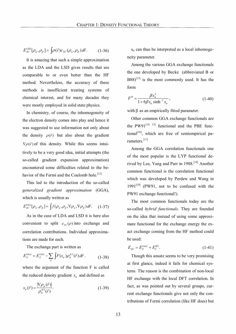
sσ can thus be interpreted as a local inhomoge-
neity parameter.
Among the various GGA exchange functionals
the one developed by Becke (abbreviated B or
B88)[13] is the most commonly used. It has the
form 2
11 6 sinhB sF
s sσ
σ σ
ββ −=
+, (1-40)
with β as an empirically fitted parameter.
Other common GGA exchange functionals are
the PW91[14, 15] functional and the PBE func-
tional[16], which are free of semiempirical pa-
rameters.[17]
Among the GGA correlation functionals one
of the most popular is the LYP functional de-
rived by Lee, Yang and Parr in 1988.[18] Another
common functional is the correlation functional
which was developed by Perdew and Wang in
1991[19] (PW91, not to be confused with the
PW91 exchange functional!).
The most common functionals today are the
so-called hybrid functionals. They are founded
on the idea that instead of using some approxi-
mate functional for the exchange energy the ex-
act exchange coming from the HF method could
be used:
.exact KSXC X CE E E= + (1-41)
Though this ansatz seems to be very promising
at first glance, indeed it fails for chemical sys-
tems. The reason is the combination of non-local
HF exchange with the local DFT correlation. In
fact, as was pointed out by several groups, cur-
rent exchange functionals give not only the con-
tributions of Fermi correlation (like HF does) but
CHAPTER 1: DENSITY FUNCTIONAL THEORY
14
also simulate the contribution of the non-
dynamical correlation. The DFT correlation
functional only includes the dynamical correla-
tion. Therefore the so-called self interaction er-
ror occurs in DFT. Nevertheless, it was found
that including only some amount of exact ex-
change in fact improves the performance of ex-
change functionals.[20] Probably the most wide-
spread functional belongs to this class. It was
developed by Becke and is abbreviated as B3[21]
because it has three parameters. Originally Becke
introduced this hybrid functional with the PW91
correlation functional[18, 21], but it became more
popular after Stephens et al. suggested to take the
LYP correlation functional instead in 1994[22]: 3 0 88(1 )
(1 ) .
B LYP LSD BXC XC XC X
LYP LSDC C
E a E a E b Ec E c E
λ== − + +
+ + − (1-42)
1.4.2. The LCAO Approach
As mentioned in the previous chapter the compu-
tational procedures to solve the Kohn-Sham
equations follow the HF method exactly. They
often make use of the LCAO expansion of the
KS molecular orbitals. LCAO (linear combina-
tion of atomic orbitals) was introduced by
Roothaan in 1951.[23] In the LCAO approach a
set of L predefined basis functions {ηµ} is used
for the expansion:
1
.L
i icµ µµ
ϕ η=
= ∑ (1-43)
Which basis functions are usually taken we
will discuss later in this section. If one inserts eq.
1-43 into eq. 1-26 one obtains
1 1 11 1
ˆ ( ) ( ) ( ).L L
KSvi v i vi v
v vf r c r c rη ε η
= =
=∑ ∑r r r (1-44)
This equation is now multiplied from the left
with an arbitrary basis function and integrated
over all space. One gets L equations
1 1 11
1 1 11
ˆ( ) ( ) ( )
( ) ( ) for 1 .
LKS
vi i vv
L
i vi vv
c r f r r dr
c r r dr i L
µ
µ
η η
ε η η
=
=
= ≤ ≤
∑ ∫
∑ ∫
r r r r
r r r (1-45)
The integral on the left hand side is called Kohn-
Sham matrix:
1 1 1ˆ( ) ( ) ( ) ,KS KS
v i vF r f r r drµ µη η= ∫r r r r (1-46)
whereas the matrix on the right hand side is the
so-called overlap matrix
1 1 1( ) ( ) .v vS r r drµ µη η= ∫r r r (1-47)
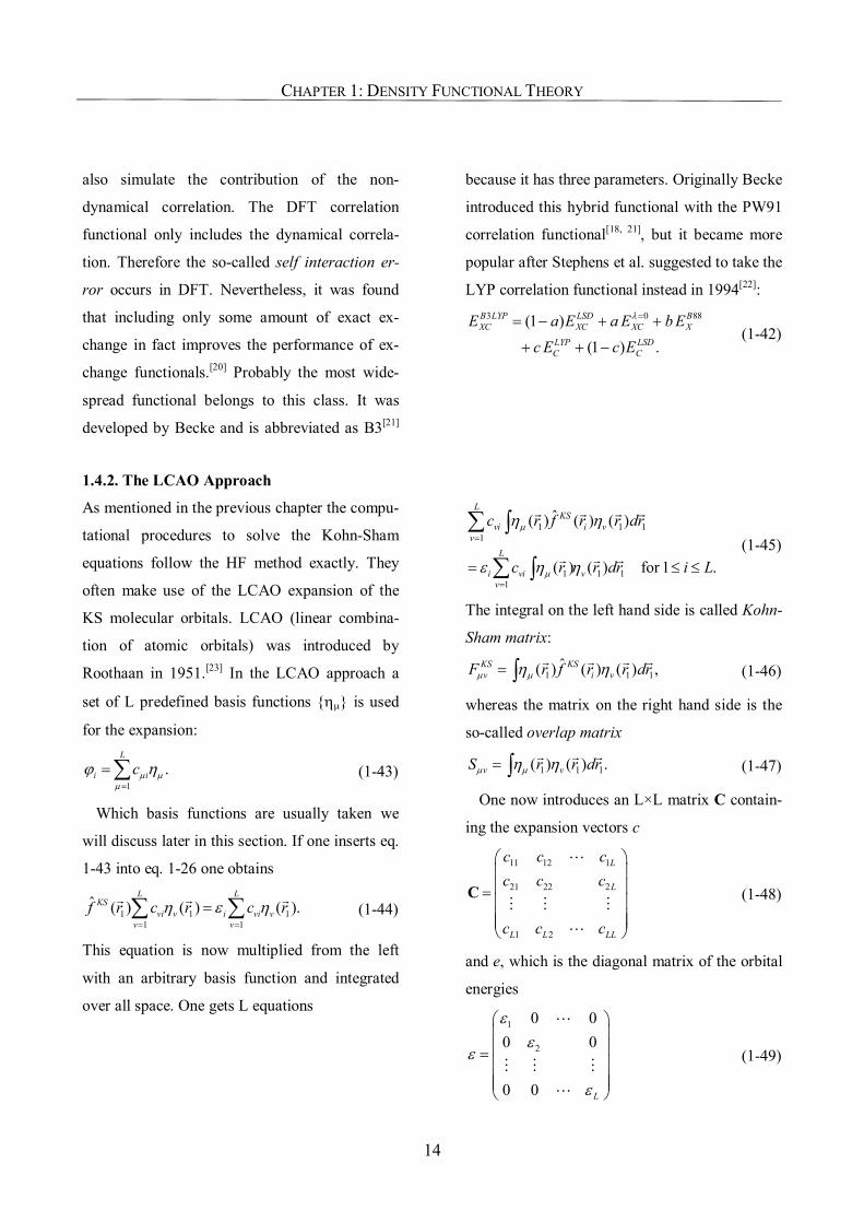
One now introduces an L×L matrix C contain-
ing the expansion vectors c
11 12 1
21 22 2
1 2
L
L
L L LL
c c cc c c
c c c
=
C
L
M M ML
(1-48)
and e, which is the diagonal matrix of the orbital
energies
1
2
0 00 0
0 0 L
εε
ε
ε
=
L
M M ML
(1-49)
CHAPTER 1: DENSITY FUNCTIONAL THEORY
15
and finally one arrives at the Roothaan-Hall
equations KS =F C SCε . (1-50)
The only difference from HF is that the original
Fock matrix F differs from the Kohn-Sham Fock
matrix FKS.
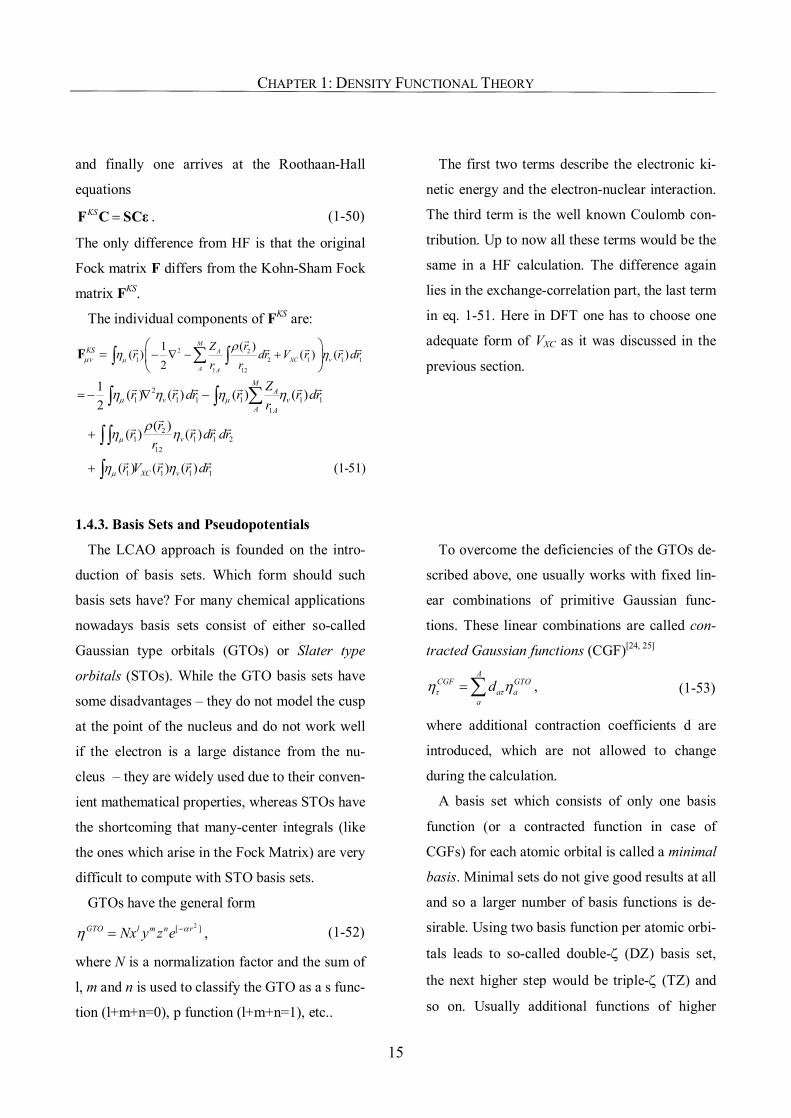
The individual components of FKS are:
2 21 2 1 1 1
1 12
21 1 1 1 1 1
1
21 1 1 2
12
1 1 1 1
( )1( ) ( ) ( )
2
1 ( ) ( ) ( ) ( )2
( )( ) ( )
( ) ( ) ( ) (1-51)
MA
XC vA A
KSv
MA
v vA A
v
XC v
Z rr dr V r r dr
r r
Zr r dr r r drr
rr r dr drr
r V r r dr
µµ
µ µ
µ
µ
ρη η
η η η η
ρη η
η η
− ∇ − +
=
= − ∇ −
+
+
∑∫ ∫
∑∫ ∫
∫ ∫
∫
Fr
r r r r r
r r r r r r
rr r r r
r r r r
The first two terms describe the electronic ki-
netic energy and the electron-nuclear interaction.
The third term is the well known Coulomb con-
tribution. Up to now all these terms would be the
same in a HF calculation. The difference again
lies in the exchange-correlation part, the last term
in eq. 1-51. Here in DFT one has to choose one
adequate form of VXC as it was discussed in the
previous section.
1.4.3. Basis Sets and Pseudopotentials
The LCAO approach is founded on the intro-
duction of basis sets. Which form should such
basis sets have? For many chemical applications
nowadays basis sets consist of either so-called
Gaussian type orbitals (GTOs) or Slater type
orbitals (STOs). While the GTO basis sets have
some disadvantages – they do not model the cusp
at the point of the nucleus and do not work well
if the electron is a large distance from the nu-
cleus – they are widely used due to their conven-
ient mathematical properties, whereas STOs have
the shortcoming that many-center integrals (like
the ones which arise in the Fock Matrix) are very
difficult to compute with STO basis sets.
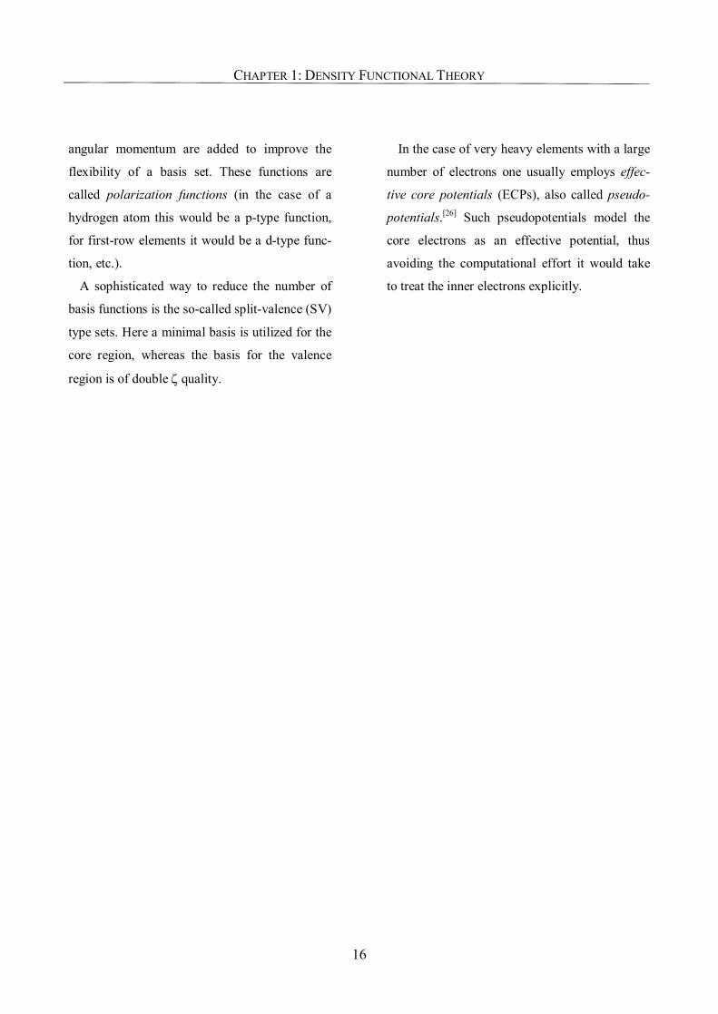
GTOs have the general form 2[ ]GTO l m n rNx y z e αη −= , (1-52)
where N is a normalization factor and the sum of
l, m and n is used to classify the GTO as a s func-
tion (l+m+n=0), p function (l+m+n=1), etc..
To overcome the deficiencies of the GTOs de-
scribed above, one usually works with fixed lin-
ear combinations of primitive Gaussian func-
tions. These linear combinations are called con-
tracted Gaussian functions (CGF)[24, 25] A
CGF GTOa a
adτ τη η= ∑ , (1-53)
where additional contraction coefficients d are
introduced, which are not allowed to change
during the calculation.
A basis set which consists of only one basis
function (or a contracted function in case of
CGFs) for each atomic orbital is called a minimal
basis. Minimal sets do not give good results at all
and so a larger number of basis functions is de-
sirable. Using two basis function per atomic orbi-
tals leads to so-called double-ζ (DZ) basis set,
the next higher step would be triple-ζ (TZ) and
so on. Usually additional functions of higher
CHAPTER 1: DENSITY FUNCTIONAL THEORY
16
angular momentum are added to improve the
flexibility of a basis set. These functions are
called polarization functions (in the case of a
hydrogen atom this would be a p-type function,
for first-row elements it would be a d-type func-
tion, etc.).
A sophisticated way to reduce the number of
basis functions is the so-called split-valence (SV)
type sets. Here a minimal basis is utilized for the
core region, whereas the basis for the valence
region is of double ζ quality.
In the case of very heavy elements with a large
number of electrons one usually employs effec-
tive core potentials (ECPs), also called pseudo-
potentials.[26] Such pseudopotentials model the
core electrons as an effective potential, thus
avoiding the computational effort it would take
to treat the inner electrons explicitly.
17
Chapter 2
Electron Paramagnetic Resonance Parameters
In this chapter we will discuss the theory of the
phenomenon of electron paramagnetic reso-
nance. We show how the electron spin arises
from the relativistic Dirac equation (though for
the purposes of this thesis we will not use the
fully relativistic Dirac Hamiltonian but the trans-
formed Breit-Pauli one) and introduce the con-
cept of the effective Spin Hamiltonian. Briefly
experimental techniques to measure the electron
paramagnetic resonance parameters will be pre-
sented. The calculation of g- and A-tensors based
on Perturbation Theory is established and ex-
plicit derivations for those two properties are
given. The theoretical formalism follows the
fundamental textbook on EPR theory written by
Harriman[1] and other textbooks.[2, 3]
In the last section we will extend the theory of
EPR parameters to cases when there is more than
one spin center in the molecule. The calculation
of exchange coupling parameters within the
framework of Noodleman’s broken-symmetry
approach will be introduced.[4, 5]
2.1. The Electron Spin
2.1.1. Where does it come from? – The Electron Spin as a Theoretical Concept
The concept of electron spin was introduced
almost at the same time as the elementary equa-
tions of quantum mechanics were discovered: in
1922 the famous Stern-Gerlach experiment
showed that there are discrete orientations of the
magnetic moment of the electron when interact-
ing with an inhomogeneous magnetic field.
Based on these results Uhlenbeck and Goud-
smith postulated in 1925 that electrons should
have an intrinsic angular momentum – the elec-
tron spin. This concept was soon incorporated
into the new theory of quantum mechanics. How-
ever, this incorporation was done only via a pos-
tulate and does not arise intrinsically from a
quantum mechanical derivation. This postulate,
made by Pauli in 1927, stated that every electron
has additionally to its spatial function φ(r) a pa-
rameter of electron spin σ. The electron spin
exists therefore as a degenerate combination of
the two states
1 0; .
0 1α β
= =
(2-1)
The spin states α and β are often also called
spin-up (↑) and spin-down (↓) respectively.
While the postulate was sound, the situation
remained unsatisfactory, as there was no explicit
theory in which the electron spin would arise
naturally and could be derived. Then Dirac con-
CHAPTER 2: ELECTRON PARAMAGNETIC RESONANCE PARAMETERS
18
nected quantum mechanics with Einstein’s spe-
cial relativity theory by writing[6]
2 2 2 2c m ci t
∂Ψ− = ± − ∇ + Ψ
∂h h . (2-2)
Dirac circumvented the problem of not know-
ing how to treat the square-root in the relativistic
Hamiltonian by setting
2 2 2 2 .m c mci
− ∇ + Ψ = ∇ +α βhh , (2-3)
where α = (αx, αy, αz) and β are Hermitian matri-
ces (Dirac matrices) with constant coefficients.
In the solution of the Dirac equation this leads to
a four-component relativistic wave function, and
therefore the Dirac equation
2.c mci t i
∂ − = ∇ + ∂ Ψ α β Ψh h (2-4)
represents a system of four partial differential
equations.
The four solutions for these equations are inter-
preted in such way that two of them represent
mostly electrons (and therefore the two spin
states arise naturally in the Dirac theory) and the
other two represent mostly positrons.
As chemistry is only interested in the electrons
and not in the positrons it is convenient to reduce
the four-component Dirac equation to a two-
component one (by formally removing the posi-
tronic contributions). Further reduction would
lead to the one-component Breit-Pauli (BP)
Hamiltonian which we will introduce in section
2.2.
2.1.2. The Effective Spin Hamiltonian
The resonances which can be experimentally
observed in an EPR spectrum are in general ana-
lyzed in terms of a phenomenological Hamilto-
nian: the effective spin Hamiltonian. This effec-
tive spin Hamiltonian (denoted ĤS) is defined as
an operator which acts only on the spin variables.
It includes all magnetic interactions coming from
the spin magnetic moments of electrons S and of
nuclei I, and the external magnetic field B. These
interactions are coupled pairwise by several cou-
pling parameters – the EPR parameters.
In the case of EPR spectroscopy a rather gen-
eral effective Hamiltonian could be written as
ˆ ˆ ˆ ˆ ˆ( , ) ( , ) ( , ) ( , ).SH H S B H S I H S S H I I= + + +
(2-5)
Throughout this thesis we will use an even
more reduced effective spin Hamiltonian which
only incorporates the two most common EPR
interactions:
ˆ ˆ ˆ( , ) ( , )S
N
H H S B H S I= +
= ⋅ ⋅ + ⋅ ⋅∑ NS g B S A I (2-6)
which are: (a) the electron Zeeman interaction
describing the coupling of the electron spin to an
external magnetic field, and (b) the hyperfine
interaction describing the coupling of the elec-
tron spin to the nuclear magnetic moment of
nucleus N. In the former interaction the coupling
parameter is called electronic g-tensor g, in the
latter one this parameter is called hyperfine ten-
sor AN.
To complete the description we will shortly
discuss two other EPR parameters which are not
so widely used as the g- and A-tensor. Neverthe-
CHAPTER 2: ELECTRON PARAMAGNETIC RESONANCE PARAMETERS
19
less, in the case when there are interactions be-
tween unpaired electrons eq. 2-6 must be aug-
mented with
ˆ ( , )H S S = ⋅ ⋅S D S , (2-7)
which describes the so-called zero field splitting.
D is called the zero field splitting tensor.
The interaction of the magnetic moments of
high spin nuclei (IN> 12 ) is called quadrupole
coupling
ˆ ( , )QN
H I I = ⋅ ⋅∑ N NN NI Q I , (2-8)
with the quadrupole coupling tensor QNN
2.1.3. Measuring the Electronic Spin
EPR spectroscopy is based on the principle
that in a magnetic field the degeneracy of the
spin states of electrons which are characterized
by the quantum number ms is lifted and transi-
tions between the spin levels can occur. These
transitions are induced by radiation with micro-
waves (the typical X-band EPR uses microwaves
with 9.5 GHz, W-band uses 95 GHz) in a mag-
netic field with the strength of several thousand
Gauss. In contrast to the free electron, unpaired
electrons in molecules interact with their envi-
ronment and the details of the measured EPR
spectra depend strongly on the character of these
interactions.[2, 3, 7, 8] This justifies the relevance of
EPR spectroscopy as an important tool for the
investigation of the molecular and electronic
structure.
Unfortunately, EPR spectroscopy is limited to
paramagnetic molecules which is the reason that
it was dwarfed for a long time by the much more
widespread NMR spectroscopy. EPR is mainly
restricted to organotransition metal radicals and
coordination complexes as well as to a limited
number of organic radicals. However, especially
in biological relevant systems often reaction
steps and species with unpaired electrons oc-
cur.[9-11] This has renewed the interest in EPR
spectroscopy in the last decades. Modern EPR
methods like high-field EPR (up to 285 GHz)
and especially the electron nuclear double reso-
nance (ENDOR) have made EPR spectroscopy a
valuable method for the investigation of elec-
tronic structure, not only but especially in bioin-
organic chemistry. We will focus primarily on
such compounds throughout this thesis. Most of
these compounds were measured in condensed
phase either as powder sample or as single crys-
tal. For both cases it is possible to introduce a
principal axes system and determine the anisot-
ropic EPR parameters. As symmetry considera-
tions are of great importance in the interpretation
of solid-state EPR we will briefly introduce the
common classification of symmetry specifica-
tions:
a) isotropic: All three components of the EPR
property are the same. This completely absence
of anisotropy can occur when the investigated
compound is spherically symmetric.
b) axial: Two principal values of the EPR ten-
sor are equal but differ from the third one, con-
ventionally they are labeled ( , , )g g g⊥ ⊥ P and
CHAPTER 2: ELECTRON PARAMAGNETIC RESONANCE PARAMETERS
20
( , , )A A A⊥ ⊥ P . This situation is found when linear
rotational symmetry about a unique axis in the
observed molecule is present. This means that all
systems where an Abelian symmetry group is
present should show axial EPR parameters .
c) rhombic: All three principal values are dif-
ferent. This is the case in molecules with non-
Abelian symmetry.
Comparing calculated with experimental data
one always has to keep in mind that environ-
mental effects can influence the values of the
EPR parameters. Additionally it is often difficult
to determine the sign of the EPR parameters out
of the experimental data.
2.2. From an Effective Spin Hamiltonian to a Quantum Mechanical One
In this thesis we will use quantum mechanical
methods to obtain the g and A coupling parame-
ters. We will mostly utilize a so-called one-
component DFT approach together with second-
order perturbation theory. An alternative to this
procedure would be the two-component DFT
approach which employs a relativistic[12] wave
function and treats the SO coupling variationally.
While this treatment would be more fundamen-
tal, it is restricted to relatively small systems and
not applicable for most chemical interesting
problems.
In the one-component approach the g- and A-
tensors can formally be obtained as second de-
rivatives of the molecular energy with respect to
the particular spin magnetic moments and/or
magnetic field: 2
0
1uv
B u v
EgB Sµ
=
∂=
∂ ∂B=S
(2-9)
and 2
,, 0N
N uvN u v
EAI S
=
∂=
∂ ∂I =S
, (2-10)
where guv and AN,uv denote the Cartesian compo-
nents of the tensors, µB is the Bohr Magneton (µB
= 12 , in the whole thesis the atomic units of the
SI system are used).
2.2.1. The Breit-Pauli Hamiltonian
To follow this procedure we need to connect
the concept of an effective spin Hamiltonian with
a “real” microscopic one. The Hamiltonian
which we will use in the following for our one-
component approach is the many-electron quasi-
relativistic Breit-Pauli (BP) Hamiltonian. The BP
Hamiltonian is derived from the Dirac equation
and consists of several distinct group of opera-
tors: electronic, nuclear and nuclear-electronic
ones:
ˆ ˆ ˆ ˆe n enH H H H= + + . (2-11)
The pure electronic term has twelve individual
contributions 12
1
ee m
mH H
=
= ∑ , (2-12)
which are:
CHAPTER 2: ELECTRON PARAMAGNETIC RESONANCE PARAMETERS
21
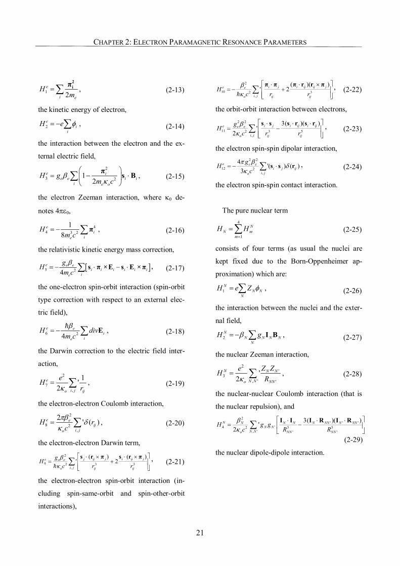
1 2e
i e
Hm
= ∑2iπ , (2-13)
the kinetic energy of electron,
2e
ii
H e φ= − ∑ , (2-14)
the interaction between the electron and the ex-
ternal electric field, 2
3 212
e ie e i i
i e o
H gm c
βκ
= − ⋅
∑ π s B , (2-15)
the electron Zeeman interaction, where κ0 de-
notes 4πε0,
44 3 2
18
ei
ie
Hm c
= − ∑π , (2-16)
the relativistic kinetic energy mass correction,
[ ]5 24e e e
i i i i i iie
gHm c
β= − ⋅ − ⋅∑ s π × E s E × π , (2-17)
the one-electron spin-orbit interaction (spin-orbit
type correction with respect to an external elec-
tric field),
6 24e e
iie
H divm cβ
= − ∑ Eh , (2-18)
the Darwin correction to the electric field inter-
action, 2
7,
1'2
e
i jo ij
eHrκ
= ∑ , (2-19)
the electron-electron Coulomb interaction, 2
8 2,
2 ' ( )e eij
i jo
H rc
πβ δκ
= ∑ , (2-20)
the electron-electron Darwin term, 2
9 2 3 3,
( ) ( )' 2j ij j i ij je e e
i jo ij ij
gHc r r
βκ
⋅ × ⋅ ×= +
∑
s r π s r πh
, (2-21)
the electron-electron spin-orbit interaction (in-
cluding spin-same-orbit and spin-other-orbit
interactions),
2
10 2 3,
( )( )' 2i j i ij ij je e
i jo ij ij
Hc r r
βκ
⋅ ⋅ ×= − +
∑
π π π r r πh
, (2-22)
the orbit-orbit interaction between electrons, 2 2
11 2 3 5,
3( )( )'
2i j i ij i ije e e
i jo ij ij
gH
c r rβ
κ
⋅ ⋅ ⋅= −
∑
s s s r s r , (2-23)
the electron spin-spin dipolar interaction, 2 2
12 2,
4 '( ) ( )3
e e ei j ij
i jo
gHc
π βδ
κ= − ⋅∑ s s r , (2-24)
the electron spin-spin contact interaction.
The pure nuclear term 4
1
NN m
mH H
=
= ∑ (2-25)
consists of four terms (as usual the nuclei are
kept fixed due to the Born-Oppenheimer ap-
proximation) which are:
1N
N NN
H e Z φ= ∑ , (2-26)
the interaction between the nuclei and the exter-
nal field,
2N
N N N NN
H gβ= − ∑ I B , (2-27)
the nuclear Zeeman interaction, 2
'3
, ' '
'2
N N N
N No NN
Z ZeHRκ
= ∑ , (2-28)
the nuclear-nuclear Coulomb interaction (that is
the nuclear repulsion), and 2
' ' '4 '2 3 5
, ' ' '
3( )( )'2
N N N N N NN N NNN N
N No NN NN
H g gc R R
βκ
⋅ ⋅ ⋅= −
∑ I I I R I R
(2-29)
the nuclear dipole-dipole interaction.
CHAPTER 2: ELECTRON PARAMAGNETIC RESONANCE PARAMETERS
22
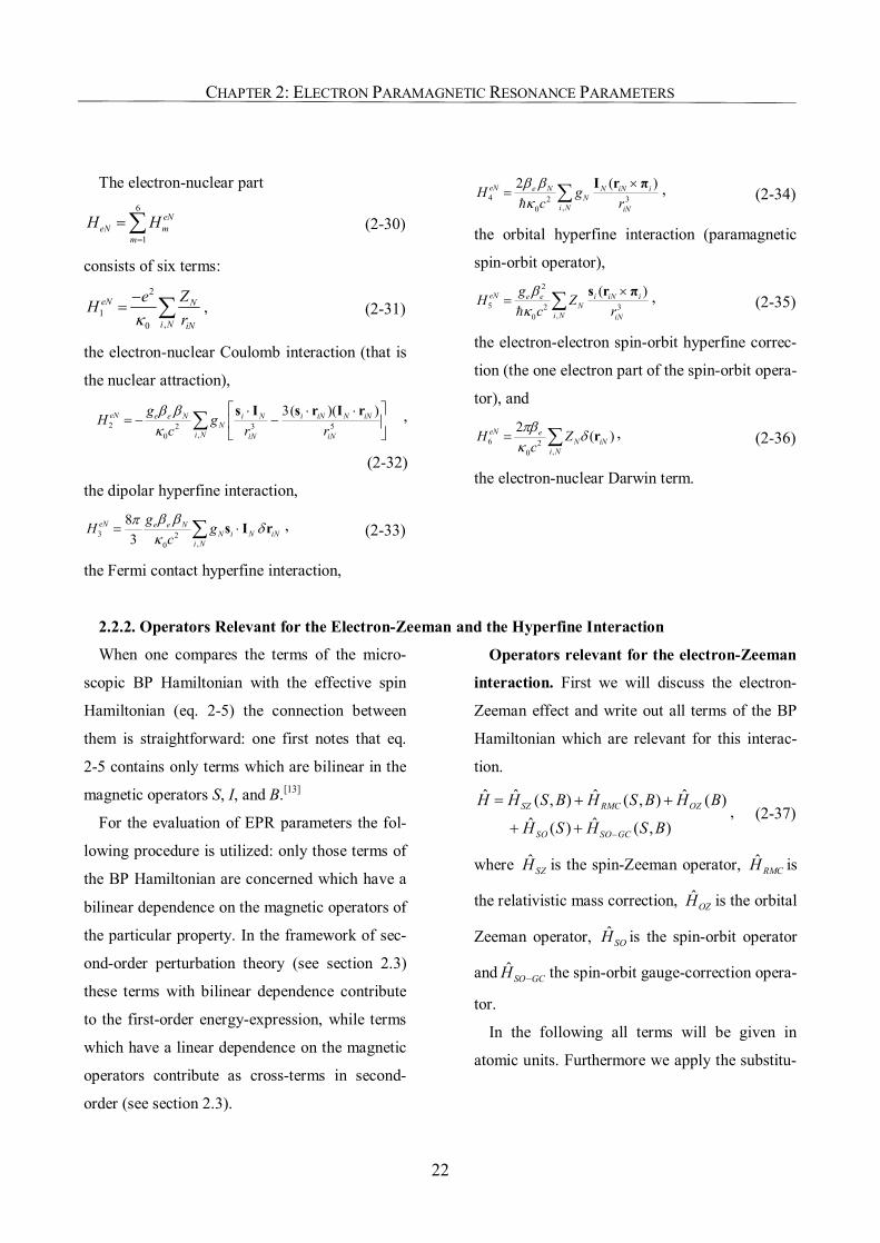
The electron-nuclear part 6
1
eNeN m
mH H
=
= ∑ (2-30)
consists of six terms: 2
1,0
eN N
i N iN
ZeHrκ
−= ∑ , (2-31)
the electron-nuclear Coulomb interaction (that is
the nuclear attraction),
2 2 3 5,0
3( )( )eN e e N i N i iN N iNN
i N iN iN
gH gc r r
β βκ
⋅ ⋅ ⋅= − −
∑ s I s r I r ,
(2-32)
the dipolar hyperfine interaction,
3 2,0
83
eN e e NN i N iN
i N
gH gc
β βπ δκ
= ⋅∑ s I r , (2-33)
the Fermi contact hyperfine interaction,
4 2 3,0
2 ( )eN e N N iN iN
i N iN
H gc r
β βκ
×= ∑ I r π
h, (2-34)
the orbital hyperfine interaction (paramagnetic
spin-orbit operator), 2
5 2 3,0
( )eN e e i iN iN
i N iN
gH Zc r
βκ
×= ∑ s r π
h, (2-35)
the electron-electron spin-orbit hyperfine correc-
tion (the one electron part of the spin-orbit opera-
tor), and
6 2,0
2 ( )eN eN iN
i NH Z
cπβ
δκ
= ∑ r , (2-36)
the electron-nuclear Darwin term.
2.2.2. Operators Relevant for the Electron-Zeeman and the Hyperfine Interaction
When one compares the terms of the micro-
scopic BP Hamiltonian with the effective spin
Hamiltonian (eq. 2-5) the connection between
them is straightforward: one first notes that eq.
2-5 contains only terms which are bilinear in the
magnetic operators S, I, and B.[13]
For the evaluation of EPR parameters the fol-
lowing procedure is utilized: only those terms of
the BP Hamiltonian are concerned which have a
bilinear dependence on the magnetic operators of
the particular property. In the framework of sec-
ond-order perturbation theory (see section 2.3)
these terms with bilinear dependence contribute
to the first-order energy-expression, while terms
which have a linear dependence on the magnetic
operators contribute as cross-terms in second-
order (see section 2.3).
Operators relevant for the electron-Zeeman
interaction. First we will discuss the electron-
Zeeman effect and write out all terms of the BP
Hamiltonian which are relevant for this interac-
tion.
ˆ ˆ ˆ ˆ( , ) ( , ) ( )ˆ ˆ( ) ( , )
SZ RMC OZ
SO SO GC
H H S B H S B H B
H S H S B−
= + +
+ +, (2-37)
where ˆSZH is the spin-Zeeman operator, ˆ
RMCH is
the relativistic mass correction, ˆOZH is the orbital
Zeeman operator, ˆSOH is the spin-orbit operator
and ˆSO GCH − the spin-orbit gauge-correction opera-
tor.
In the following all terms will be given in
atomic units. Furthermore we apply the substitu-
CHAPTER 2: ELECTRON PARAMAGNETIC RESONANCE PARAMETERS
23
tion 1cα = , where α is the fine structure con-
stant.
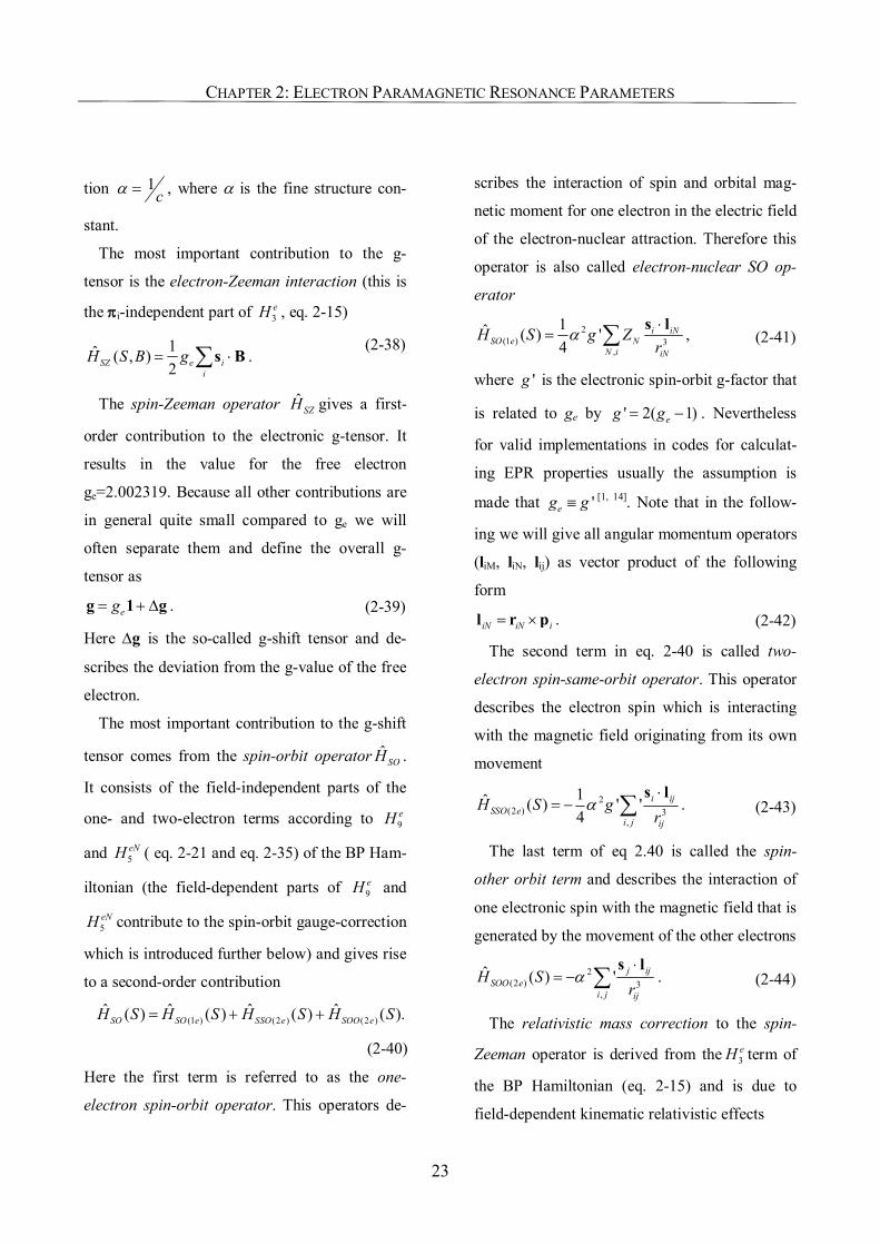
The most important contribution to the g-
tensor is the electron-Zeeman interaction (this is
the πi-independent part of 3eH , eq. 2-15)
1ˆ ( , )2SZ e i
iH S B g= ⋅∑s B .
(2-38)
The spin-Zeeman operator ˆSZH gives a first-
order contribution to the electronic g-tensor. It
results in the value for the free electron
ge=2.002319. Because all other contributions are
in general quite small compared to ge we will
often separate them and define the overall g-
tensor as
eg= + ∆g 1 g . (2-39)
Here ∆g is the so-called g-shift tensor and de-
scribes the deviation from the g-value of the free
electron.
The most important contribution to the g-shift
tensor comes from the spin-orbit operator ˆSOH .
It consists of the field-independent parts of the
one- and two-electron terms according to 9eH
and 5eNH ( eq. 2-21 and eq. 2-35) of the BP Ham-
iltonian (the field-dependent parts of 9eH and
5eNH contribute to the spin-orbit gauge-correction
which is introduced further below) and gives rise
to a second-order contribution
(1 ) (2 ) (2 )ˆ ˆ ˆ ˆ( ) ( ) ( ) ( ).SO SO e SSO e SOO eH S H S H S H S= + +
(2-40)
Here the first term is referred to as the one-
electron spin-orbit operator. This operators de-
scribes the interaction of spin and orbital mag-
netic moment for one electron in the electric field
of the electron-nuclear attraction. Therefore this
operator is also called electron-nuclear SO op-
erator
2(1 ) 3
,
1ˆ ( ) '4
i iNSO e N
N i iN
H S g Zr
α⋅
= ∑ s l , (2-41)
where 'g is the electronic spin-orbit g-factor that
is related to ge by ' 2( 1)eg g= − . Nevertheless
for valid implementations in codes for calculat-
ing EPR properties usually the assumption is
made that 'eg g≡ [1, 14]. Note that in the follow-
ing we will give all angular momentum operators
(liM, liN, lij) as vector product of the following
form
iN iN i= ×l r p . (2-42)
The second term in eq. 2-40 is called two-
electron spin-same-orbit operator. This operator
describes the electron spin which is interacting
with the magnetic field originating from its own
movement
2(2 ) 3
,
1ˆ ( ) ' '4
i ijSSO e
i j ij
H S gr
α⋅
= − ∑s l
. (2-43)
The last term of eq 2.40 is called the spin-
other orbit term and describes the interaction of
one electronic spin with the magnetic field that is
generated by the movement of the other electrons
2(2 ) 3
,
ˆ ( ) ' j ijSOO e
i j ij
H Sr
α⋅
= − ∑s l
. (2-44)
The relativistic mass correction to the spin-
Zeeman operator is derived from the 3eH term of
the BP Hamiltonian (eq. 2-15) and is due to
field-dependent kinematic relativistic effects
CHAPTER 2: ELECTRON PARAMAGNETIC RESONANCE PARAMETERS
24
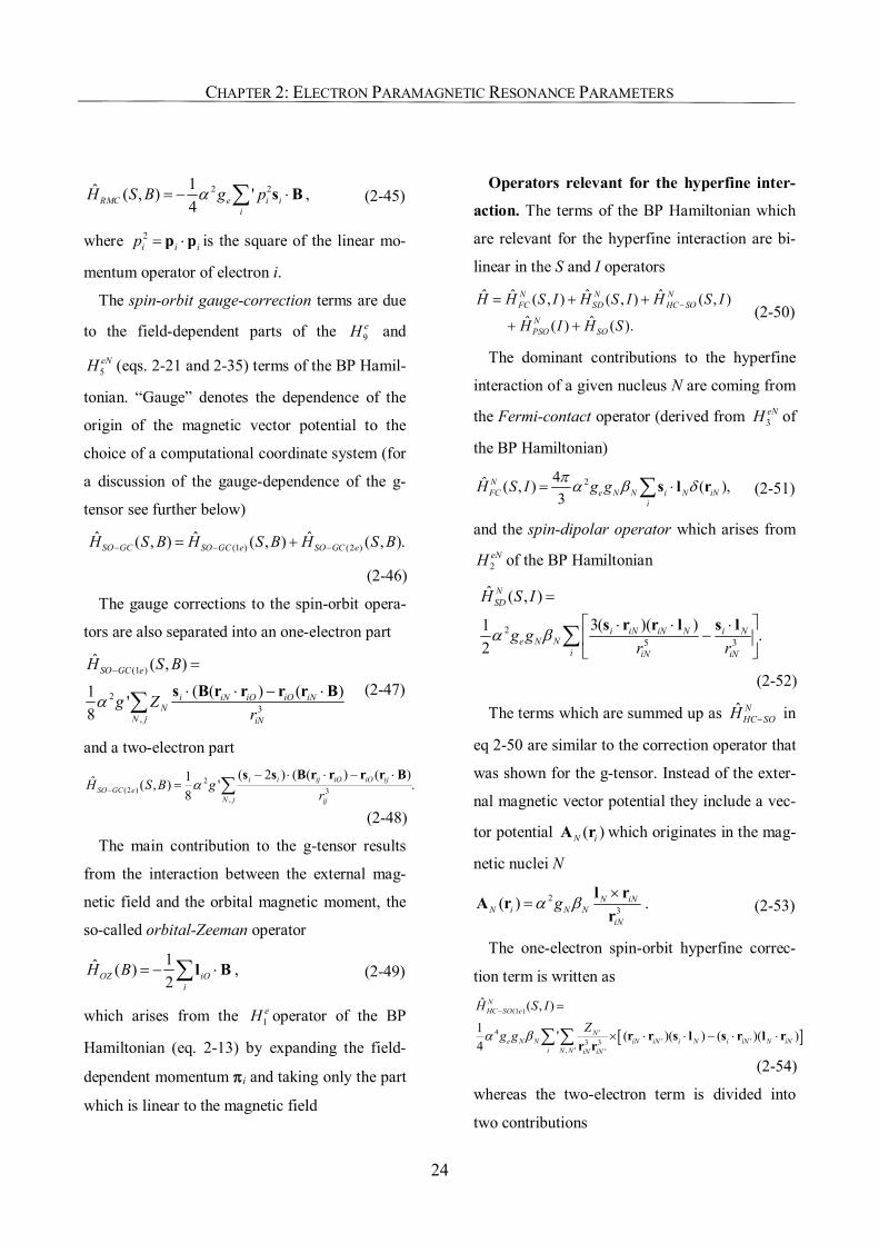
2 21ˆ ( , ) '4RMC e i i
iH S B g pα= − ⋅∑ s B , (2-45)
where 2i i ip = ⋅p p is the square of the linear mo-
mentum operator of electron i.
The spin-orbit gauge-correction terms are due
to the field-dependent parts of the 9eH and
5eNH (eqs. 2-21 and 2-35) terms of the BP Hamil-
tonian. “Gauge” denotes the dependence of the
origin of the magnetic vector potential to the
choice of a computational coordinate system (for
a discussion of the gauge-dependence of the g-
tensor see further below)
(1 ) (2 )ˆ ˆ ˆ( , ) ( , ) ( , ).SO GC SO GC e SO GC eH S B H S B H S B− − −= +
(2-46)
The gauge corrections to the spin-orbit opera-
tors are also separated into an one-electron part
(1 )
23
,
ˆ ( , )
( ( ) ( )1 '8
SO GC e
i iN iO iO iNN
N j iN
H S B
g Zr
α
− =
⋅ ⋅ − ⋅∑ s B r r r r B (2-47)
and a two-electron part
2(2 ) 3
,
( 2 ) ( ( ) ( )1ˆ ( , ) ' .8
i i ij iO iO ijSO GC e
N j ij
H S B gr
α−
− ⋅ ⋅ − ⋅= ∑
s s B r r r r B
(2-48)
The main contribution to the g-tensor results
from the interaction between the external mag-
netic field and the orbital magnetic moment, the
so-called orbital-Zeeman operator
1ˆ ( )2OZ iO
iH B = − ⋅∑l B , (2-49)
which arises from the 1eH operator of the BP
Hamiltonian (eq. 2-13) by expanding the field-
dependent momentum πi and taking only the part
which is linear to the magnetic field
Operators relevant for the hyperfine inter-
action. The terms of the BP Hamiltonian which
are relevant for the hyperfine interaction are bi-
linear in the S and I operators
ˆ ˆ ˆ ˆ( , ) ( , ) ( , )ˆ ˆ( ) ( ).
N N NFC SD HC SO
NPSO SO
H H S I H S I H S I
H I H S−= + +
+ + (2-50)
The dominant contributions to the hyperfine
interaction of a given nucleus N are coming from
the Fermi-contact operator (derived from 3eNH of
the BP Hamiltonian)
24ˆ ( , ) ( ),3
NFC e N N i N iN
i
H S I g gπ α β δ= ⋅∑s l r (2-51)
and the spin-dipolar operator which arises from
2eNH of the BP Hamiltonian
25 3
ˆ ( , )
3( )( )1 .2
NSD
i iN iN N i Ne N N
i iN iN
H S I
g gr r
α β
=
⋅ ⋅ ⋅−
∑ s r r l s l
(2-52)
The terms which are summed up as ˆ NHC SOH − in
eq 2-50 are similar to the correction operator that
was shown for the g-tensor. Instead of the exter-
nal magnetic vector potential they include a vec-
tor potential ( )N iA r which originates in the mag-
netic nuclei N
23( ) N iN
N i N NiN
gα β×
=l rA r
r. (2-53)
The one-electron spin-orbit hyperfine correc-
tion term is written as
[ ]
(1 )
4 '' '3 3
, ' '
ˆ ( , )
1 ' ( )( ) ( )( )4
NHC SO e
Ne N N iN iN i N i iN N iN
i N N iN iN
H S IZg gα β
− =
× ⋅ ⋅ − ⋅ ⋅∑ ∑ r r s l s r l rr r
(2-54)
whereas the two-electron term is divided into
two contributions
CHAPTER 2: ELECTRON PARAMAGNETIC RESONANCE PARAMETERS
25
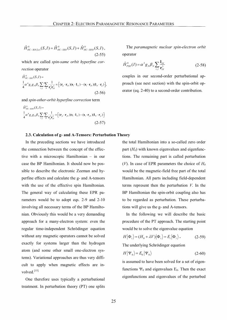
(2 )ˆ ˆ ˆ( , ) ( , ) ( , )N N N
HC SO e HC SSO HC SOOH S I H S I H S I− − −= + , (2-55)
which are called spin-same orbit hyperfine cor-
rection operator
43 3
,
ˆ ( , )1 1' ( )( ) ( )( ) ,4
NHC SSO
e N N ij iN i N i iN N iji j N ij iN
H S I
g gα β
− =
× ⋅ ⋅ − ⋅ ⋅ ∑ ∑ r r s l s r l rr r
(2-56)
and spin-other-orbit hyperfine correction term
43 3
,
ˆ ( , )1 1' ( )( ) ( )( )4
NHC SOO
e N N ji jN i N i jN N jii j N ij iN
H S I
g gα β
− =
× ⋅ ⋅ − ⋅ ⋅ ∑ ∑ r r s l s r l rr r
(2-57)
The paramagnetic nuclear spin-electron orbit
operator
23
,
ˆ ( )N iNPSO N N
i j iN
H I gα β= ∑ lr
(2-58)
couples in our second-order perturbational ap-
proach (see next section) with the spin-orbit op-
erator (eq. 2-40) to a second-order contribution.
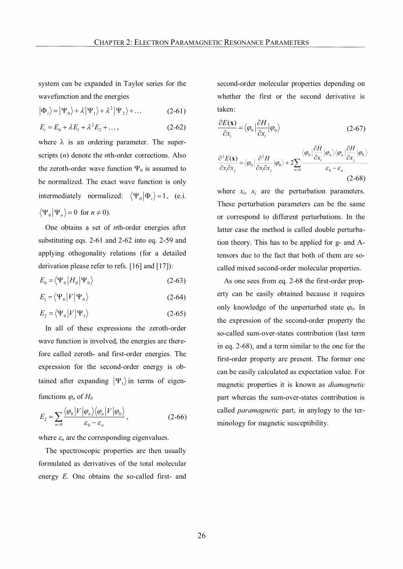
2.3. Calculation of g- and A-Tensors: Perturbation Theory
In the preceding sections we have introduced
the connection between the concept of the effec-
tive with a microscopic Hamiltonian – in our
case the BP Hamiltonian. It should now be pos-
sible to describe the electronic Zeeman and hy-
perfine effects and calculate the g- and A-tensors
with the use of the effective spin Hamiltonian.
The general way of calculating these EPR pa-
rameters would be to adopt eqs. 2-9 and 2-10
involving all necessary terms of the BP Hamilto-
nian. Obviously this would be a very demanding
approach for a many-electron system: even the
regular time-independent Schrödinger equation
without any magnetic operators cannot be solved
exactly for systems larger than the hydrogen
atom (and some other small one-electron sys-
tems). Variational approaches are thus very diffi-
cult to apply when magnetic effects are in-
volved.[15]
One therefore uses typically a perturbational
treatment. In perturbation theory (PT) one splits
the total Hamiltonian into a so-called zero order
part (H0) with known eigenvalues and eigenfunc-
tions. The remaining part is called perturbation
(V). In case of EPR parameters the choice of H0
would be the magnetic-field free part of the total
Hamiltonian. All parts including field-dependent
terms represent then the perturbation V. In the
BP Hamiltonian the spin-orbit coupling also has
to be regarded as perturbation. These perturba-
tions will give us the g- and A-tensors.
In the following we will describe the basic
procedure of the PT approach. The starting point
would be to solve the eigenvalue equation
0( )i i i iH H V EλΦ = + Φ = Φ . (2-59)
The underlying Schrödinger equation
0 0 0H EΨ = Ψ (2-60)
is assumed to have been solved for a set of eigen-
functions Ψ0 and eigenvalues E0. Then the exact
eigenfunctions and eigenvalues of the perturbed
CHAPTER 2: ELECTRON PARAMAGNETIC RESONANCE PARAMETERS
26
system can be expanded in Taylor series for the
wavefunction and the energies 2
0 1 2i λ λΦ = Ψ + Ψ + Ψ +… (2-61)
20 1 2iE E E Eλ λ= + + +… , (2-62)
where λ is an ordering parameter. The super-
scripts (n) denote the nth-order corrections. Also
the zeroth-order wave function Ψ0 is assumed to
be normalized. The exact wave function is only
intermediately normalized: 0 1iΨ Φ = , (e.i.
0 0nΨ Ψ = for n ≠ 0).
One obtains a set of nth-order energies after
substituting eqs. 2-61 and 2-62 into eq. 2-59 and
applying othogonality relations (for a detailed
derivation please refer to refs. [16] and [17]):
0 0 0 0E H= Ψ Ψ (2-63)
1 0 0E V= Ψ Ψ (2-64)
2 0 1E V= Ψ Ψ (2-65)
In all of these expressions the zeroth-order
wave function is involved, the energies are there-
fore called zeroth- and first-order energies. The
expression for the second-order energy is ob-
tained after expanding 1Ψ in terms of eigen-
functions ϕn of H0
0 02
0 0
n n
n n
V VE
ϕ ϕ ϕ ϕε ε>
=−∑ , (2-66)
where εn are the corresponding eigenvalues.
The spectroscopic properties are then usually
formulated as derivatives of the total molecular
energy E. One obtains the so-called first- and
second-order molecular properties depending on
whether the first or the second derivative is
taken:
0 0( )
i i
E Hx x
ϕ ϕ∂ ∂=
∂ ∂x (2-67)
0 02 2
0 00 0
( ) 2n n
i j
ni j i j n
H Hx xE H
x x x x
ϕ ϕ ϕ ϕϕ ϕ
ε ε>
∂ ∂∂ ∂∂ ∂
= +∂ ∂ ∂ ∂ −∑x
(2-68)
where xi, xj are the perturbation parameters.
These perturbation parameters can be the same
or correspond to different perturbations. In the
latter case the method is called double perturba-
tion theory. This has to be applied for g- and A-
tensors due to the fact that both of them are so-
called mixed second-order molecular properties.
As one sees from eq. 2-68 the first-order prop-
erty can be easily obtained because it requires
only knowledge of the unperturbed state ϕ0. In
the expression of the second-order property the
so-called sum-over-states contribution (last term
in eq. 2-68), and a term similar to the one for the
first-order property are present. The former one
can be easily calculated as expectation value. For
magnetic properties it is known as diamagnetic
part whereas the sum-over-states contribution is
called paramagnetic part, in anylogy to the ter-
minology for magnetic susceptibility.
CHAPTER 2: ELECTRON PARAMAGNETIC RESONANCE PARAMETERS
27
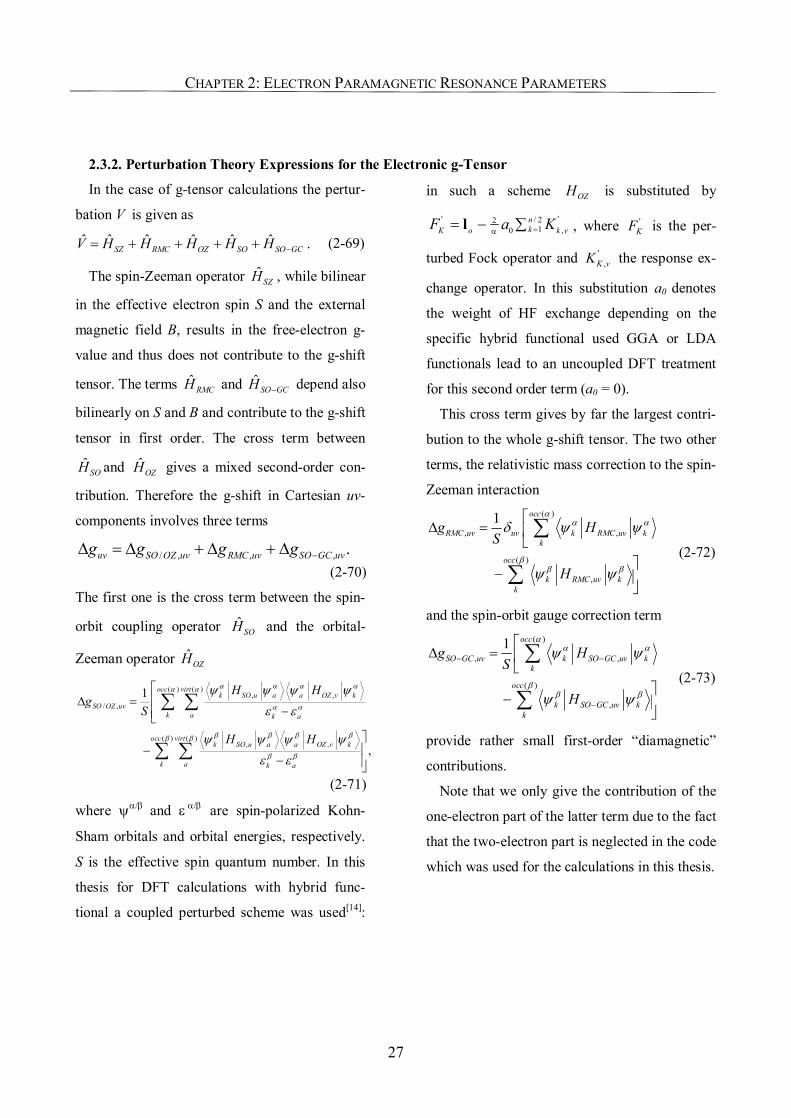
2.3.2. Perturbation Theory Expressions for the Electronic g-Tensor
In the case of g-tensor calculations the pertur-
bation V is given as
ˆ ˆ ˆ ˆ ˆ ˆSZ RMC OZ SO SO GCV H H H H H −= + + + + . (2-69)
The spin-Zeeman operator ˆSZH , while bilinear
in the effective electron spin S and the external
magnetic field B, results in the free-electron g-
value and thus does not contribute to the g-shift
tensor. The terms ˆRMCH and ˆ
SO GCH − depend also
bilinearly on S and B and contribute to the g-shift
tensor in first order. The cross term between
ˆSOH and ˆ
OZH gives a mixed second-order con-
tribution. Therefore the g-shift in Cartesian uv-
components involves three terms
/ , , , .uv SO OZ uv RMC uv SO GC uvg g g g −∆ = ∆ + ∆ + ∆(2-70)
The first one is the cross term between the spin-
orbit coupling operator ˆSOH and the orbital-
Zeeman operator ˆOZH
( ) ( ), ,
/ ,
( ) ( ), ,
1
,
occ virtk SO u a a OZ v k
SO OZ uvk a k a
occ virtk SO u a a OZ v k
k a k a
H Hg
S
H H
α α α αα α
α α
β β β ββ β
β β
ψ ψ ψ ψ
ε ε
ψ ψ ψ ψ
ε ε
∆ =
−−
−
∑ ∑
∑ ∑
(2-71)
where ψα/β and ε α/β are spin-polarized Kohn-
Sham orbitals and orbital energies, respectively.
S is the effective spin quantum number. In this
thesis for DFT calculations with hybrid func-
tional a coupled perturbed scheme was used[14]:
in such a scheme OZH is substituted by
' '/ 2210 ,
nkK o k vF a K=α= − ∑l , where '
KF is the per-
turbed Fock operator and ',K vK the response ex-
change operator. In this substitution a0 denotes
the weight of HF exchange depending on the
specific hybrid functional used GGA or LDA
functionals lead to an uncoupled DFT treatment
for this second order term (a0 = 0).
This cross term gives by far the largest contri-
bution to the whole g-shift tensor. The two other
terms, the relativistic mass correction to the spin-
Zeeman interaction ( )
, ,
( )
,
1 occ
RMC uv uv k RMC uv kk
occ
k RMC uv kk
g HS
H
αα α
ββ β
δ ψ ψ
ψ ψ
∆ =
−
∑
∑ (2-72)
and the spin-orbit gauge correction term ( )
, ,
( )
,
1 occ
SO GC uv k SO GC uv kk
occ
k SO GC uv kk
g HS
H
αα α
ββ β
ψ ψ
ψ ψ
− −
−
∆ =
−
∑
∑ (2-73)
provide rather small first-order “diamagnetic”
contributions.
Note that we only give the contribution of the
one-electron part of the latter term due to the fact
that the two-electron part is neglected in the code
which was used for the calculations in this thesis.
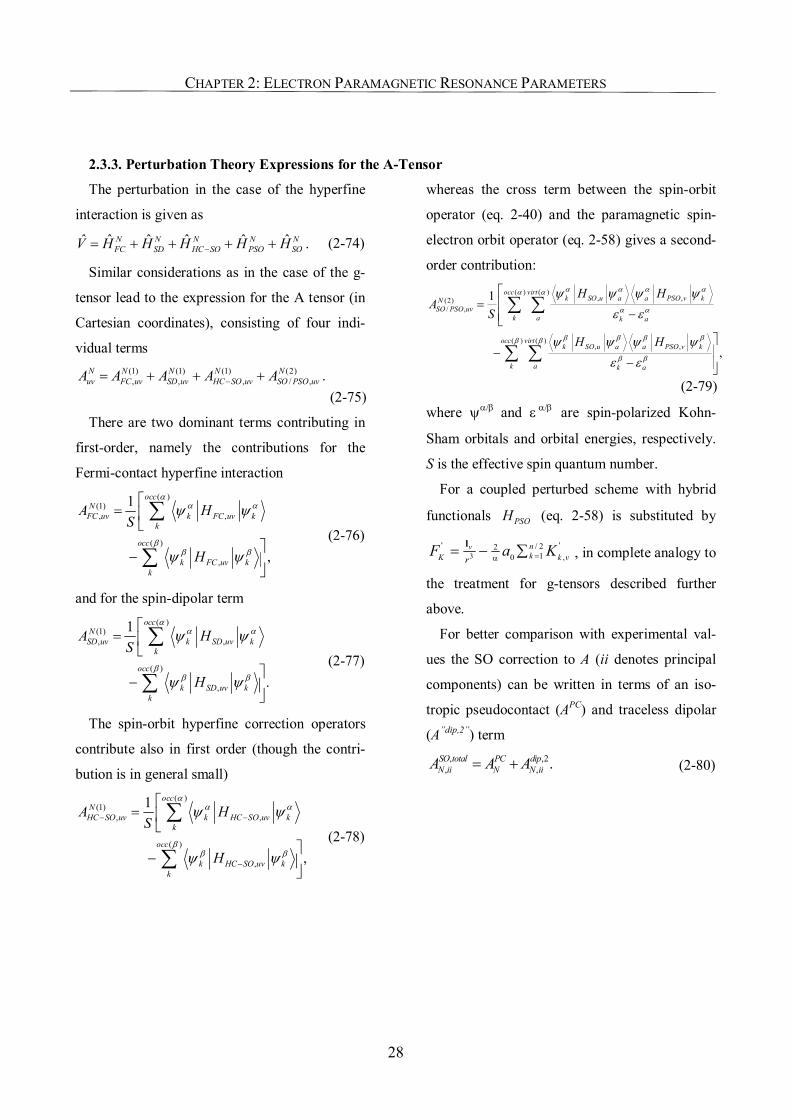
CHAPTER 2: ELECTRON PARAMAGNETIC RESONANCE PARAMETERS
28
2.3.3. Perturbation Theory Expressions for the A-Tensor
The perturbation in the case of the hyperfine
interaction is given as
ˆ ˆ ˆ ˆ ˆ ˆN N N N NFC SD HC SO PSO SOV H H H H H−= + + + + . (2-74)
Similar considerations as in the case of the g-
tensor lead to the expression for the A tensor (in
Cartesian coordinates), consisting of four indi-
vidual terms (1) (1) (1) (2), , , / , .N N N N N
uv FC uv SD uv HC SO uv SO PSO uvA A A A A−= + + +(2-75)
There are two dominant terms contributing in
first-order, namely the contributions for the
Fermi-contact hyperfine interaction ( )
(1), ,
( )
,
1
,
occN
FC uv k FC uv kk
occ
k FC uv kk
A HS
H
αα α
ββ β
ψ ψ
ψ ψ
=
−
∑
∑ (2-76)
and for the spin-dipolar term ( )
(1), ,
( )
,
1
.
occN
SD uv k SD uv kk
occ
k SD uv kk
A HS
H
αα α
ββ β
ψ ψ
ψ ψ
=
−
∑
∑ (2-77)
The spin-orbit hyperfine correction operators
contribute also in first order (though the contri-
bution is in general small) ( )
(1), ,
( )
,
1
,
occN
HC SO uv k HC SO uv kk
occ
k HC SO uv kk
A HS
H
αα α
ββ β
ψ ψ
ψ ψ
− −
−
=
−
∑
∑ (2-78)
whereas the cross term between the spin-orbit
operator (eq. 2-40) and the paramagnetic spin-
electron orbit operator (eq. 2-58) gives a second-
order contribution:
( ) ( ), ,(2)
/ ,
( ) ( ), ,
1
,
occ virtk SO u a a PSO v kN
SO PSO uvk a k a
occ virtk SO u a a PSO v k
k a k a
H HA
S
H H
α α α αα α
α α
β β β ββ β
β β
ψ ψ ψ ψ
ε ε
ψ ψ ψ ψ
ε ε
=
−−
−
∑ ∑
∑ ∑
(2-79)
where ψα/β and ε α/β are spin-polarized Kohn-
Sham orbitals and orbital energies, respectively.
S is the effective spin quantum number.
For a coupled perturbed scheme with hybrid
functionals PSOH (eq. 2-58) is substituted by
3' '/ 22
10 ,v n
kK k vrF a K=α
= − ∑l, in complete analogy to
the treatment for g-tensors described further
above.
For better comparison with experimental val-
ues the SO correction to A (ii denotes principal
components) can be written in terms of an iso-
tropic pseudocontact (APC) and traceless dipolar
(A”dip,2”) term , ,2
, , .SO total PC dipN ii N N iiA A A= + (2-80)
CHAPTER 2: ELECTRON PARAMAGNETIC RESONANCE PARAMETERS
29
2.4. SO Operators and the Gauge Origin of the g-Tensor
In this section we will shortly discuss two
practical problems which occur when calculating
g-tensors and the SO corrections to the A tensor.
The first is the SO operator in the BP Hamilto-
nian as it is shown in eq. 2-41, eq. 2-43 and eq.
2-44. In its two-electron form it is quite complex
and difficult to handle for implementation in
computer codes. Therefore several approxima-
tions have been suggested, for example the
treatment as an effective one-electron operator
where the nuclear charge ZN is fitted with an
effective charge ZN,eff (see eq. 2-41).[18, 19] In this
thesis the atomic mean-field (AMFI) method is
used to approximate the SO operators.[20, 21]
AMFI includes both the one-electron as well as
the two-electron SO operator but instead of cal-
culating all integrals explicitly it utilizes a super-
position of effective atomic SO operators. AMFI
is therefore highly adapted for the calculation of
large systems. Furthermore the one-center nature
of the AMFI operator allows it to breakdown the
∆gSO/OZ term into SO contributions coming from
individual atoms or fragments of the molecule.
In the cases of very heavy elements also spin-
orbit effective core potentials (SO-ECP) were
used.[22] These SO-ECPs treat only the valence
electrons explicitly and model the core electrons
by an effective potential.
The second difficulty one has to deal with in g-
tensor calculations is the dependence of this
property on the gauge origin of the magnetic
vector potential. Sophisticated methods to dis-
tribute the gauge have been developed, namely
the individual gauges for localized orbitals
(IGLO)[23, 24] or the gauge including atomic orbi-
tals (GIAO)[25]. Nevertheless, usually the gauge
dependence is small and calculations with a
common gauge origin at the center of charge or
at the central atom of a transition metal complex
give adequate results.[26-28] Throughout this thesis
only common gauge origins are used.
2.5. More than one Spin Center: Exchange Interaction
2.5.1. The Heisenberg-Dirac-van-Vleck Hamiltonian
The theoretical treatment described above
deals with the situation when one spin center in a
molecule is present or if one spin is delocalized
over the molecule. The description becomes
more difficult if there are distinct regions in a
molecule with discrete magnetic centers which
interact with each other via a weak bonding. This
occurs frequently in inorganic magnets and in
coordination compounds with more than one
paramagnetic metal centers or coordination com-
pounds with paramagnetic organic ligands and
one or more paramagnetic metal centers.[29]
In such cases one usually utilizes the so-called
Heisenberg-Dirac-van-Vleck (HDVV) Hamilto-
nian
ˆ ˆexHDVV ij i j
i jH J
>
= ⋅∑ S S , (2-81)
CHAPTER 2: ELECTRON PARAMAGNETIC RESONANCE PARAMETERS
30
where the exchange coupling constant Jex de-
scribes an isotropic interaction between para-
magnetic centers.[30]
Occasionally this HDVV Hamiltonian is not
sufficient and one has to add additional terms
due to the zero-field splitting and biquadratic
correction terms to describe non-linear interac-
tions between the paramagnetic centers. Such
non-Heisenberg terms are often regarded as first-
order perturbations to the energy which one ob-
tains when applying the HDVV Hamiltonian.[31]
The energy of each spin state as a function of J
can the be written as
( ) ( 1)2JE S S S= + . (2-82)
The HDVV Hamiltonian could be strictly ap-
plied only when the spins are localized on the
magnetic centers. For cases with delocalized spin
it has to be extended by the so-called double-
exchange parameter B
1( ) ( 1) ( )2 2JE S S S B S= + ± + . (2-83)
2.5.2. The Broken-Symmetry Approach for Calculating J Values
The calculation of the exchange coupling pa-
rameter J encounters a difficulty: the exchange
interaction is an extremely weak chemical bond-
ing which is strongly influenced by the presence
of static and dynamic electron correlation effects.
Therefore post-HF techniques would be needed
to achieve an adequate description of this inter-
action. Another way which works also for single-
determinant (SD) approaches like DFT or HF
was developed by Noodleman.[4, 5] The so-called
broken-symmetry (bs) approach relates the en-
ergy of an bs SD – which is not an eigenstate of
the spin operator S2 – to the energy of a pure spin
state.
The bs approach requires the calculation of the
energy of several SDs (for each bs state and ad-
ditionally the hs state, which is the only state that
can be correctly described by a SD). It was
shown (a detailed derivation is found for exam-
ple in ref. [29]) that the bs state can be approxi-
mated as
( )BS SS
A SΨ = Ψ∑ , (2-84)
where ( )A S denotes the weighted average of
different spin states S.
For a binuclear system AB with centers A and
B having the same spin eq. 2-81 can be written
as
ˆ ˆexHDVV A BH J= ⋅S S . (2-85)
The difference between the highest spin state
and the bs state according to eqs. 2-82 and 2-84
is then given by max
max max max 10
( ) ( 1) ( ) ( 1) ,2
S
bsS
JE S E S S A S S S=
− = + − +
∑
(2-86)
with Smax = SA + SB.
With the help of the condition max
1 max( ) ( 1)S
SA S S S S+ =∑ (2-87)
one gets
CHAPTER 2: ELECTRON PARAMAGNETIC RESONANCE PARAMETERS
31
max2max
( )2
bsE S EJS
−= . (2-88)
For the general case, when SA ≠ SB eq. 2-86
becomes
2hs bs
A B
E EJS S−
= , (2-89)
with Ehs denoting the high spin state with S(hs) =
SA + SB.
Additionally we will show the equations for a
C2-symmetrical compound with three spin cen-
ters, because we will encounter such a species in
chapter 8. For such a case the HDVV-Hamil-
tonian can be written as
1 2 2 3 1 3ˆ ˆ ˆ ˆ ˆ ˆ( ) ( )HDVVH J J ′= ⋅ + ⋅ + ⋅S S S S S S , (2-90)
where Si denotes the three spin centers of these
molecules, with each Si = 12 . The energies of the
spin states are then:
,1
,2
3a) ;2 2 41b) ;2 2 41c) ; .2 4
hs
bs
bs
J JMs E
J JMs E
JMs E
′= ± = +
′= ± = − +
′= ± = −
(2-91)
With the help of these relations J and J’ can be
computed as energy differences according to
a bE J−∆ = , (2-92)
2 2a cJ JE −
′∆ = + , (2-93)
2 2b cJ JE −
′∆ = − + . (2-94)
The HDVV-Hamiltonian can be further ex-
tended to molecules containing several paramag-
netic centers (such systems are usually referred
to as “molecular magnets”). For the derivation of
the HDVV-Hamiltonian of such molecular mag-
nets please refer for instance to refs. [32] and
[33].

32
33
Chapter 3:
Spin-Orbit Corrections
to Hyperfine Coupling Tensors[1]
3.1. Introduction
In this chapter we will report the first valida-
tion study of a new implementation of SO cor-
rections to HFC tensors in our in-house MAG-
ReSpect code[2], mainly for transition metal
complexes (but also some small diatomics), com-
paring GGA and hybrid functionals.
Several second-order perturbation theory DFT
approaches to calculate SO corrections to HFC
tensors have been proposed. While most imple-
mentations have relied on semi-empirical one-
electron SO operators,[3-6] Arbuznikov et al. from
our group have reported[7] the first calculations
using accurate ab initio approximations to the
full microscopic one- and two-electron Breit-
Pauli SO Hamiltonian. These were (a) the all-
electron atomic mean-field approximation,[8] and
(b) SO pseudopotentials (“effective core poten-
tials”, SO-ECPs).[9-11][12] Test calculations of
HFC tensors in a series of model systems, using
local density (LDA) and generalized gradient-
correction (GGA) exchange-correlation func-
tionals, have provided reasonable agreement
between these two approaches, as well as with
experiment, provided that the underlying nonre-
lativistic (NR) parts of the HFC tensor were
computed accurately.
The implementation of ref. [7] suffered still
from limitations in the used deMon-KS[13, 14] and
deMon-NMR-EPR[15] codes. These were (a) the
restriction of both orbital basis sets and auxiliary
basis sets for the fit of electron density and ex-
change-correlation potential to angular momen-
tum l ≤ 2, and (b) restriction to LDA and GGA
functionals, due to the lack of four-center two-
electron integrals. This precludes the use of hy-
brid functionals that include a fraction of exact
exchange. As results of Neese[4] suggested larger
SO corrections to HFC tensors in transition metal
complexes when using hybrid functionals, the
use of such functionals seems to be mandatory to
achieve a potentially better agreement with ex-
periment.
CHAPTER 3: SPIN-ORBIT CORRECTIONS TO HYPERFINE COUPLING TENSORS
34
3.2. Computational Details
In contrast to the previous deMon implementa-
tion[7], the MAG-ReSpect implementation does
not have to rely on fitting of charge density or
exchange-correlation functional but compute
four-center two-electron integrals explicitly. The
BP86 GGA functional[16-18] and the B3PW91
hybrid functional[19, 20] were compared. In addi-
tion, in some cases the B3LYP functional[19, 21]
was used for comparison in calculations of the
NR part of the HFC tensors. In the latter calcula-
tions, the SCF part was done with the Gaus-
sian98 program[22], and the Kohn-Sham orbitals
were transferred to MAG-ReSpect by suitable
interface routines[23].
For 3d transition metals, a (15s11p6d)/-
[9s7p4d] basis constructed specifically for HFC
calculations[24] has been used. Ligand atoms were
treated by Huzinaga-Kutzelnigg-type basis sets
BII and BIII.[25, 26] For a series of diatomic we
compare all-electron and ECP calculations (the
SCF part was done with the Gaussian98 pro-
gram[22] in this cases). For the all-electron calcu-
lations we have used the BIII type basis[25, 26] for
the lighter atoms, with basis sets by Fægri[27] for
the heavier elements in an analogous BIII-type
contraction (denoted as FIII). Scalar relativistic
ECPs and corresponding SO-ECPs for Ga, In, Rh
(small-core definition), as well as for Br and I (7-
valence-electron treatment) were taken from refs. [9-12].
The effective one-electron/one-center mean-
field SO operators were computed with the
AMFI program[28]. In cases where ECPs and SO-
ECPs were used on the heavy atoms, AMFI SO
operators were employed on the light atoms.
In the case of metal carbonyl and manganese
complexes, molecular structures used for the
hyperfine structure calculations were taken from
experiment where available. Where not, the
DFT-optimized structures of ref. [24] were used.
Structures of Cu complexes have been optimized
in unrestricted Kohn-Sham calculations with the
BP86 functional using the Turbomole 5.6 pro-
gram[29] and TZVP basis sets[30] for all atoms.
The Coulomb term was approximated by the
resolution of the identity (RI) method (density
fitting with a TZVP auxiliary basis set)[31]. We
verified that the structures obtained are closely
similar to those used by Neese[4]. Structures of
the series of diatomics studied are those em-
ployed and discussed in ref. [7].
All HFC tensor results are reported in MHz
3.3. Results and Discussion
3.3.1. Carbonyl Complexes: Comparison to Semiempirical SO Corrections
In Table 3.1, comparison is made for a number
of carbonyl complexes to first-order NR results
of ref. [3], augmented by semi-empirical SO
corrections. Both the BP86 GGA functional and
the hybrid B3PW91 functional have been used.
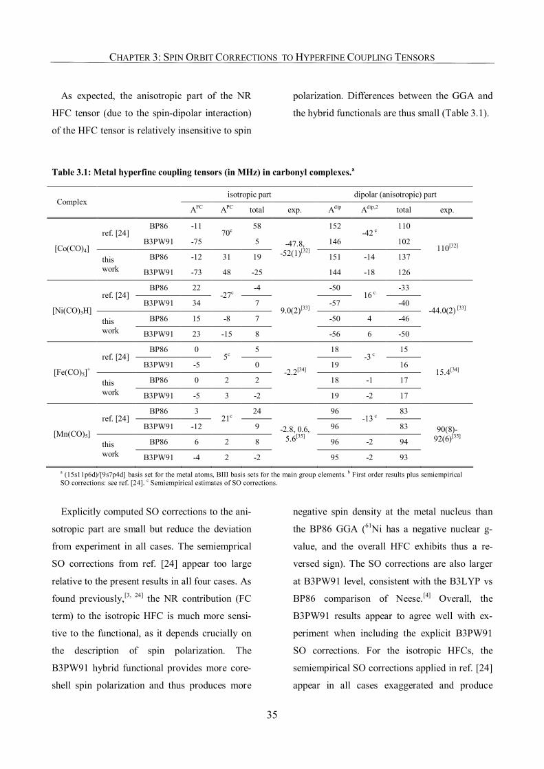
CHAPTER 3: SPIN ORBIT CORRECTIONS TO HYPERFINE COUPLING TENSORS
35
As expected, the anisotropic part of the NR
HFC tensor (due to the spin-dipolar interaction)
of the HFC tensor is relatively insensitive to spin
polarization. Differences between the GGA and
the hybrid functionals are thus small (Table 3.1).
Table 3.1: Metal hyperfine coupling tensors (in MHz) in carbonyl complexes.a
isotropic part dipolar (anisotropic) part Complex
AFC APC total exp. Adip Adip,2 total exp.
BP86 -11 58 152 110 ref. [24]
B3PW91 -75 70c
5 146 -42 c
102
BP86 -12 31 19 151 -14 137 [Co(CO)4]
this work B3PW91 -73 48 -25
-47.8, -52(1)[32]
144 -18 126
110[32]
BP86 22 -4 -50 -33 ref. [24]
B3PW91 34 -27c
7 -57 16 c
-40
BP86 15 -8 7 -50 4 -46 [Ni(CO)3H]
this work B3PW91 23 -15 8
9.0(2)[33]
-56 6 -50
-44.0(2) [33]
BP86 0 5 18 15 ref. [24]
B3PW91 -5 5c
0 19 -3 c
16
BP86 0 2 2 18 -1 17 [Fe(CO)5]+
this work B3PW91 -5 3 -2
-2.2[34]
19 -2 17
15.4[34]
BP86 3 24 96 83 ref. [24]
B3PW91 -12 21c
9 96 -13 c
83
BP86 6 2 8 96 -2 94 [Mn(CO)5]
this work B3PW91 -4 2 -2
-2.8, 0.6, 5.6[35]
95 -2 93
90(8)-92(6)[35]
a (15s11p6d)/[9s7p4d] basis set for the metal atoms, BIII basis sets for the main group elements. b First order results plus semiempirical SO corrections: see ref. [24]. c Semiempirical estimates of SO corrections.
Explicitly computed SO corrections to the ani-
sotropic part are small but reduce the deviation
from experiment in all cases. The semiemprical
SO corrections from ref. [24] appear too large
relative to the present results in all four cases. As
found previously,[3, 24] the NR contribution (FC
term) to the isotropic HFC is much more sensi-
tive to the functional, as it depends crucially on
the description of spin polarization. The
B3PW91 hybrid functional provides more core-
shell spin polarization and thus produces more
negative spin density at the metal nucleus than
the BP86 GGA (61Ni has a negative nuclear g-
value, and the overall HFC exhibits thus a re-
versed sign). The SO corrections are also larger
at B3PW91 level, consistent with the B3LYP vs
BP86 comparison of Neese.[4] Overall, the
B3PW91 results appear to agree well with ex-
periment when including the explicit B3PW91
SO corrections. For the isotropic HFCs, the
semiempirical SO corrections applied in ref. [24]
appear in all cases exaggerated and produce
CHAPTER 3: SPIN ORBIT CORRECTIONS TO HYPERFINE COUPLING TENSORS
36
overall worse agreement with experiment com-
pared to the corrections computed here explic-
itly. As discussed previously,[3, 24] this may partly
be due to the neglect of hybridization between
metal d-, s-, and p-orbitals, the use of Mulliken
analyses in estimating d-populations, as well as
other approximations used in applying the classi-
cal perturbation formulae.
In particular, we had argued that the SO cor-
rection for [Mn(CO)5] is probably overestimated
due to the small coefficient of the 2zd orbital in
the SOMO.[3, 24] This is confirmed by the present,
much smaller SO corrections. Similarly, the SO
corrections were thought to be too large for
[Ni(CO)3H], as confirmed by the present results.
Significantly smaller SO corrections in the pre-
sent, more quantitative treatment are also obvi-
ous for [Co(CO)4].
3.3.2. Copper Complexes
Neese has studied a number of different copper
complexes with O–, N– and S–ligands to validate
his approach for calculating HFC tensors with
semi-empirical SO operators, using the BP86 and
B3LYP functionals.[4] Here we used our own
approach with the BP86 GGA functional and the
B3PW91 hybrid functional for the same set of
species (see Table 3.2).
In these complexes, SO corrections are obvi-
ously of the same order of magnitude as the NR
contributions. Their inclusion is thus absolutely
mandatory for accurate calculations of the metal
HFC tensors. Scalar relativistic effects, which are
not incorporated here, are expected to give addi-
tionally contributions in the range of 5-10%.[36]
With SO corrections taken into account, results
with hybrid functionals are a significant im-
provement over the GGA results when compar-
ing to experiment, both in the present study and
in Neese’s investigation (the sign of the experi-
mental A-tensor was not determined in all cases
but is always negative where known). This is due
to enhanced core-shell spin-polarization contri-
butions to the FC term (cf. ref. [24]), but also to
enhanced SO contributions. The general im-
provement of the agreement with experiment by
inclusion of SO corrections is shown clearly for
both isotropic and dipolar components of the
HFC tensors in Figures 3.1 and 3.2, albeit this
improvement is far less obvious when using the
BP86 GGA functional (Figure 3.1) than with the
B3PW91 hybrid functional (Figure 3.2). No
problems with spin contamination are encoun-
tered, and thus the use of hybrid functionals ap-
pears to be justified.
While our BP86 results agree closely with
those of Neese, our B3PW91 data deviate nota-
bly from his B3LYP results, particularly for the
isotropic component. In general our B3PW91
data for these tensor component appear to be in
better agreement with experiment, whereas the
dipolar components come out similar (see Table
3.2). Closer inspection reveals that the differ-
ences arise mainly from the FC term and not so
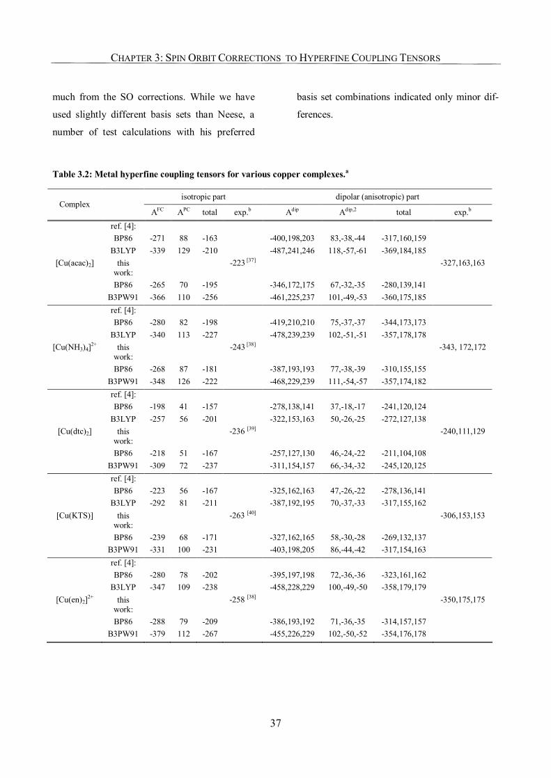
CHAPTER 3: SPIN ORBIT CORRECTIONS TO HYPERFINE COUPLING TENSORS
37
much from the SO corrections. While we have
used slightly different basis sets than Neese, a
number of test calculations with his preferred
basis set combinations indicated only minor dif-
ferences.
Table 3.2: Metal hyperfine coupling tensors for various copper complexes.a
isotropic part dipolar (anisotropic) part Complex
AFC APC total exp.b Adip Adip,2 total exp.b
[Cu(acac)2]
ref. [4]: BP86
B3LYP this
work: BP86
B3PW91
-271 -339
-265 -366
88 129
70 110
-163 -210
-195 -256
-223 [37]
-400,198,203 -487,241,246
-346,172,175 -461,225,237
83,-38,-44
118,-57,-61
67,-32,-35 101,-49,-53
-317,160,159 -369,184,185
-280,139,141 -360,175,185
-327,163,163
[Cu(NH3)4]2+
ref. [4]: BP86
B3LYP this
work: BP86
B3PW91
-280 -340
-268 -348
82 113
87 126
-198 -227
-181 -222
-243 [38]
-419,210,210 -478,239,239
-387,193,193 -468,229,239
75,-37,-37
102,-51,-51
77,-38,-39 111,-54,-57
-344,173,173 -357,178,178
-310,155,155 -357,174,182
-343, 172,172
[Cu(dtc)2]
ref. [4]: BP86
B3LYP this
work: BP86
B3PW91
-198 -257
-218 -309
41 56
51 72
-157 -201
-167 -237
-236 [39]
-278,138,141 -322,153,163
-257,127,130 -311,154,157
37,-18,-17 50,-26,-25
46,-24,-22 66,-34,-32
-241,120,124 -272,127,138
-211,104,108 -245,120,125
-240,111,129
[Cu(KTS)]
ref. [4]: BP86
B3LYP this
work: BP86
B3PW91
-223 -292
-239 -331
56 81
68 100
-167 -211
-171 -231
-263 [40]
-325,162,163 -387,192,195
-327,162,165 -403,198,205
47,-26,-22 70,-37,-33
58,-30,-28 86,-44,-42
-278,136,141 -317,155,162
-269,132,137 -317,154,163
-306,153,153
[Cu(en)2]2+
ref. [4]: BP86
B3LYP this
work: BP86
B3PW91
-280 -347
-288 -379
78 109
79 112
-202 -238
-209 -267
-258 [38]
-395,197,198 -458,228,229
-386,193,192 -455,226,229
72,-36,-36
100,-49,-50
71,-36,-35 102,-50,-52
-323,161,162 -358,179,179
-314,157,157 -354,176,178
-350,175,175
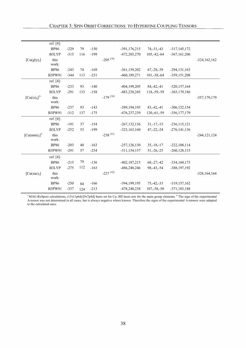
CHAPTER 3: SPIN ORBIT CORRECTIONS TO HYPERFINE COUPLING TENSORS
38
[Cu(gly)2]
ref. [4]: BP86
B3LYP this
work: BP86
B3PW91
-229 -315
-243 -344
79 116
74 113
-150 -199
-169 -231
-205 [38]
-391,176,215 -472,203,270
-361,159,202 -460,189,271
74,-31,-43
105,-42,-64
67,-28,-39 101,-38,-64
-317,145,172 -367,161,206
-294,131,163 -359,151,208
-324,162,162
[Cu(iz)4]2+
ref. [4]: BP86
B3LYP this
work: BP86
B3PW91
-233 -291
-237 -312
93 133
93 137
-140 -158
-143 -175
-179 [38]
-404,199,205 -483,238,245
-389,194,195 -476,237,239
84,-42,-41
118,-59,-59
83,-42,-41 120,-61,-59
-320,157,164 -365,179,186
-306,152,154 -356,177,179
-357,179,179
[Cu(mnt)2]2-
ref. [4]: BP86
B3LYP this
work: BP86
B3PW91
-191 -252
-203 -291
37 53
40 57
-154 -199
-163 -234
-238 [41]
-267,132,136 -323,163,160
-257,126,130 -311,154,157
31,-17,-15 47,-22,-24
35,-18,-17 51,-26,-25
-236,115,121 -276,141,136
-222,108,114 -260,128,133
-244,121,124
[Cu(sac)2]
ref. [4]: BP86
B3LYP this
work: BP86
B3PW91
-215 -275
-250 -337
79 112
84 124
-136 -163
-166 -213
-227 [42]
-402,187,215 -486,240,246
-394,199,195 -478,240,238
68,-27,-42 98,-43,-54
75,-42,-33 107,-58,-50
-334,160,173 -388,197,192
-319,157,162 -371,183,188
-328,164,164
a MAG-ReSpect calculations, (15s11p6d)/[9s7p4d] basis set for Cu, BII basis sets for the main group elements. b The sign of the experimental A-tensor was not determined in all cases, but is always negative where known. Therefore the signs of the experimental A-tensors were adapted to the calculated ones.
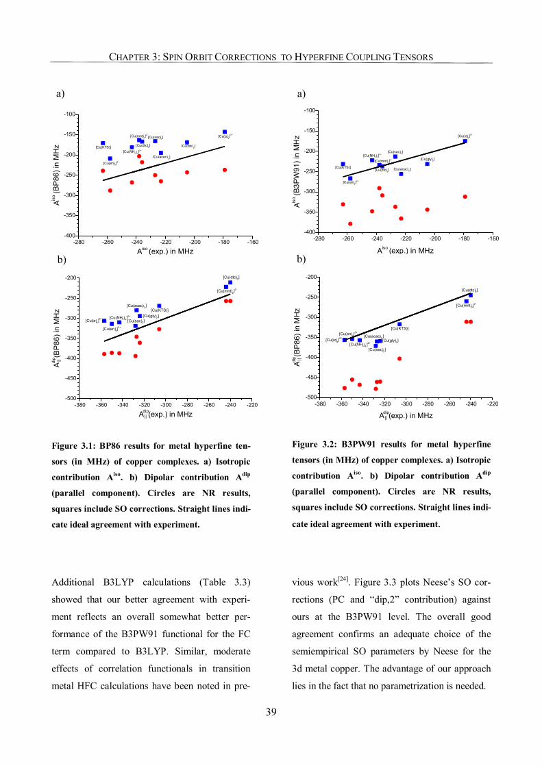
CHAPTER 3: SPIN ORBIT CORRECTIONS TO HYPERFINE COUPLING TENSORS
39
-280 -260 -240 -220 -200 -180 -160-400
-350
-300
-250
-200
-150
-100
[Cu(mnt)2]2-
[Cu(dtc)2]
[Cu(iz)4]2+
[Cu(gly)2]
[Cu(acac)2]
[Cu(NH3)4 ]2+[Cu(KTS)]
[Cu(sac)2 ]
[Cu(en)2]2+
Aiso (exp.) in MHz
Aiso (B
P86
) in
MH
z
a)
-380 -360 -340 -320 -300 -280 -260 -240 -220-500
-450
-400
-350
-300
-250
-200
Adip (exp.) in MHz||
Adip (B
P86
) in
MH
z||
[Cu(mnt)2]2-
[Cu(dtc)2]
[Cu(iz)4]2+
[Cu(gly)2 ]
[Cu(acac)2 ]
[Cu(NH3)4 ]2+
[Cu(KTS)]
[Cu(sac)2]
[Cu(en)2]2+
b)
Figure 3.1: BP86 results for metal hyperfine ten-
sors (in MHz) of copper complexes. a) Isotropic
contribution Aiso. b) Dipolar contribution Adip
(parallel component). Circles are NR results,
squares include SO corrections. Straight lines indi-
cate ideal agreement with experiment.
-280 -260 -240 -220 -200 -180 -160-400
-350
-300
-250
-200
-150
-100
[Cu(mnt)2]2-
[Cu(dtc)2]
[Cu(iz)4]2+
[Cu(gly)2]
[Cu(acac)2]
[Cu(NH3)4 ]2+
[Cu(KTS)]
[Cu(sac)2 ]
[Cu(en)2]2+
Aiso (exp.) in MHz
Aiso (B
3PW
91) i
n M
Hz
a)
-380 -360 -340 -320 -300 -280 -260 -240 -220-500
-450
-400
-350
-300
-250
-200
[Cu(mnt)2]2-
[Cu(dtc)2]
[Cu(iz)4]2+
[Cu(gly)2][Cu(acac)2 ]
[Cu(NH3)4 ]2+
[Cu(KTS)]
[Cu(sac)2]
[Cu(en)2]2+
Adip (exp.) in MHz||
Adip (B
P86)
in M
Hz
||
b)
Figure 3.2: B3PW91 results for metal hyperfine
tensors (in MHz) of copper complexes. a) Isotropic
contribution Aiso. b) Dipolar contribution Adip
(parallel component). Circles are NR results,
squares include SO corrections. Straight lines indi-
cate ideal agreement with experiment.
Additional B3LYP calculations (Table 3.3)
showed that our better agreement with experi-
ment reflects an overall somewhat better per-
formance of the B3PW91 functional for the FC
term compared to B3LYP. Similar, moderate
effects of correlation functionals in transition
metal HFC calculations have been noted in pre-
vious work[24]. Figure 3.3 plots Neese’s SO cor-
rections (PC and “dip,2” contribution) against
ours at the B3PW91 level. The overall good
agreement confirms an adequate choice of the
semiempirical SO parameters by Neese for the
3d metal copper. The advantage of our approach
lies in the fact that no parametrization is needed.
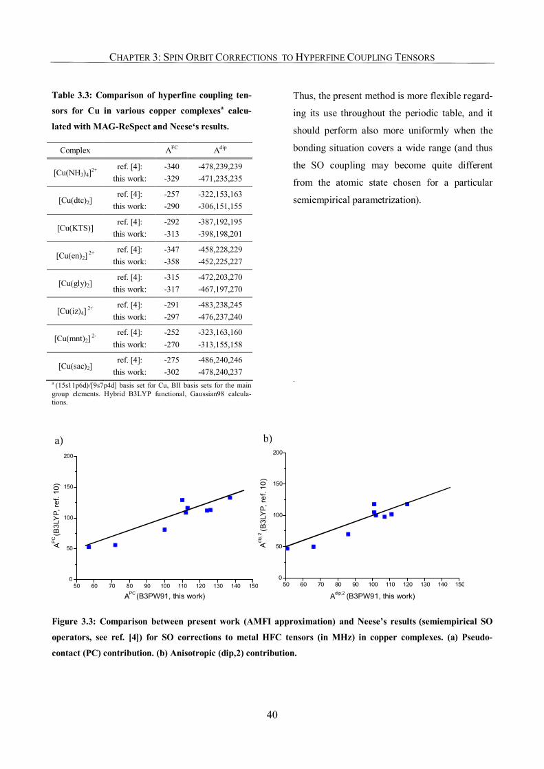
CHAPTER 3: SPIN ORBIT CORRECTIONS TO HYPERFINE COUPLING TENSORS
40
Table 3.3: Comparison of hyperfine coupling ten-
sors for Cu in various copper complexesa calcu-
lated with MAG-ReSpect and Neese‘s results.
Complex AFC Adip
[Cu(NH3)4]2+ ref. [4]:
this work: -340 -329
-478,239,239 -471,235,235
[Cu(dtc)2] ref. [4]:
this work: -257 -290
-322,153,163 -306,151,155
[Cu(KTS)] ref. [4]:
this work: -292 -313
-387,192,195 -398,198,201
[Cu(en)2] 2+ ref. [4]:
this work: -347 -358
-458,228,229 -452,225,227
[Cu(gly)2] ref. [4]:
this work: -315 -317
-472,203,270 -467,197,270
[Cu(iz)4] 2+ ref. [4]:
this work: -291 -297
-483,238,245 -476,237,240
[Cu(mnt)2] 2- ref. [4]:
this work: -252 -270
-323,163,160 -313,155,158
[Cu(sac)2] ref. [4]:
this work: -275 -302
-486,240,246 -478,240,237
a (15s11p6d)/[9s7p4d] basis set for Cu, BII basis sets for the main group elements. Hybrid B3LYP functional, Gaussian98 calcula-tions.
Thus, the present method is more flexible regard-
ing its use throughout the periodic table, and it
should perform also more uniformly when the
bonding situation covers a wide range (and thus
the SO coupling may become quite different
from the atomic state chosen for a particular
semiempirical parametrization).
.
50 60 70 80 90 100 110 120 130 140 1500
50
100
150
200
APC (B3PW91, this work)
APC (B
3LY
P, re
f. 10
)
a)
50 60 70 80 90 100 110 120 130 140 1500
50
100
150
200
Adip,2 (B3PW91, this work)
(B3L
YP,
ref.
10)
Adip,
2
b)
Figure 3.3: Comparison between present work (AMFI approximation) and Neese’s results (semiempirical SO
operators, see ref. [4]) for SO corrections to metal HFC tensors (in MHz) in copper complexes. (a) Pseudo-
contact (PC) contribution. (b) Anisotropic (dip,2) contribution.
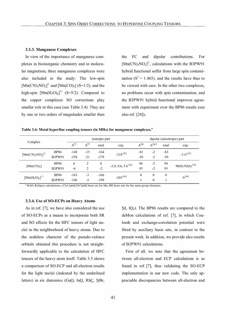
CHAPTER 3: SPIN ORBIT CORRECTIONS TO HYPERFINE COUPLING TENSORS
41
3.3.3. Manganese Complexes
In view of the importance of manganese com-
plexes in bioinorganic chemistry and in molecu-
lar magnetism, three manganese complexes were
also included in the study: The low-spin
[Mn(CN)5NO2]2- and [Mn(CO)5] (S=1/2), and the
high-spin [Mn(H2O)6]2+ (S=5/2). Compared to
the copper complexes SO corrections play
smaller role in this case (see Table 3.4). They are
by one or two orders of magnitudes smaller than
the FC and dipolar contributions. For
[Mn(CN)5NO2]2-, calculations with the B3PW91
hybrid functional suffer from large spin contami-
nation (S2 = 1.465), and the results have thus to
be viewed with care. In the other two complexes,
no problems occur with spin contamination, and
the B3PW91 hybrid functional improves agree-
ment with experiment over the BP86 results (see
also ref. [24]).
Table 3.4: Metal hyperfine coupling tensors (in MHz) for manganese complexes.a
isotropic part dipolar (anisotropic) part Complex
AFC APC total exp. Adip Adip,2 total exp.
[Mn(CN)5NO2] 2- BP86
B3PW91 -148 -258
-15 -21
-164 -279
-218 [43] -81 -56
-2 -3
-83 -59
-115 [43]
[Mn(CO)5] BP86
B3PW91 6 -4
2 2
8 -2
-2.8, 0.6, 5.6 [35] 96 95
-2 -2
94 93
90(8)-92(6) [35]
[Mn(H2O)6] 2+ BP86
B3PW91 -163 -196
-3 -3
-166 -199
-245 [44] 0 1
0 0
0 1
0 [44]
a MAG-ReSpect calculations, (15s11p6d)/[9s7p4d] basis set for Mn, BII basis sets for the main group elements.
3.3.4. Use of SO-ECPs on Heavy Atoms
As in ref. [7], we have also considered the use
of SO-ECPs as a means to incorporate both SR
and SO effects for the HFC tensors of light nu-
clei in the neighborhood of heavy atoms. Due to
the nodeless character of the pseudo-valence
orbitals obtained this procedure is not straight-
forwardly applicable to the calculation of HFC
tensors of the heavy atom itself. Table 3.5 shows
a comparison of SO-ECP and all-electron results
for the light nuclei (indcated by the underlined
letters) in six diatomics (GaO, InO, RhC, NBr,
NI, IO2). The BP86 results are compared to the
deMon calculations of ref. [7], in which Cou-
lomb and exchange-correlation potential were
fitted by auxiliary basis sets, in contrast to the
present work. In addition, we provide also results
of B3PW91 calculations.
First of all, we note that the agreement be-
tween all-electron and ECP calculations is as
found in ref. [7], thus validating the SO-ECP
implementation in our new code. The only ap-
preciable discrepancies between all-electron and
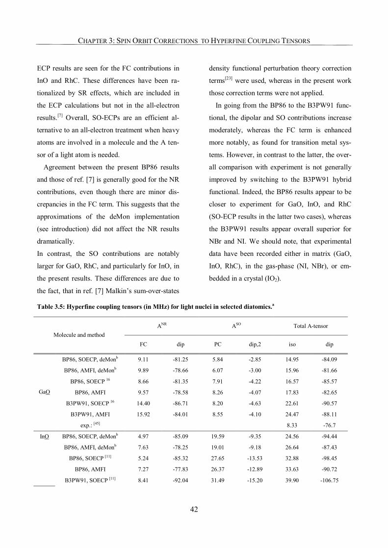
CHAPTER 3: SPIN ORBIT CORRECTIONS TO HYPERFINE COUPLING TENSORS
42
ECP results are seen for the FC contributions in
InO and RhC. These differences have been ra-
tionalized by SR effects, which are included in
the ECP calculations but not in the all-electron
results.[7] Overall, SO-ECPs are an efficient al-
ternative to an all-electron treatment when heavy
atoms are involved in a molecule and the A ten-
sor of a light atom is needed.
Agreement between the present BP86 results
and those of ref. [7] is generally good for the NR
contributions, even though there are minor dis-
crepancies in the FC term. This suggests that the
approximations of the deMon implementation
(see introduction) did not affect the NR results
dramatically.
In contrast, the SO contributions are notably
larger for GaO, RhC, and particularly for InO, in
the present results. These differences are due to
the fact, that in ref. [7] Malkin’s sum-over-states
density functional perturbation theory correction
terms[23] were used, whereas in the present work
those correction terms were not applied.
In going from the BP86 to the B3PW91 func-
tional, the dipolar and SO contributions increase
moderately, whereas the FC term is enhanced
more notably, as found for transition metal sys-
tems. However, in contrast to the latter, the over-
all comparison with experiment is not generally
improved by switching to the B3PW91 hybrid
functional. Indeed, the BP86 results appear to be
closer to experiment for GaO, InO, and RhC
(SO-ECP results in the latter two cases), whereas
the B3PW91 results appear overall superior for
NBr and NI. We should note, that experimental
data have been recorded either in matrix (GaO,
InO, RhC), in the gas-phase (NI, NBr), or em-
bedded in a crystal (IO2).
Table 3.5: Hyperfine coupling tensors (in MHz) for light nuclei in selected diatomics.a
ANR ASO Total A-tensor Molecule and method
FC dip PC dip,2 iso dip
BP86, SOECP, deMonb 9.11 -81.25 5.84 -2.85 14.95 -84.09
BP86, AMFI, deMonb 9.89 -78.66 6.07 -3.00 15.96 -81.66
BP86, SOECP 16 8.66 -81.35 7.91 -4.22 16.57 -85.57
BP86, AMFI 9.57 -78.58 8.26 -4.07 17.83 -82.65
B3PW91, SOECP 16 14.40 -86.71 8.20 -4.63 22.61 -90.57
B3PW91, AMFI 15.92 -84.01 8.55 -4.10 24.47 -88.11
GaO
exp.: [45] 8.33 -76.7
BP86, SOECP, deMonb 4.97 -85.09 19.59 -9.35 24.56 -94.44
BP86, AMFI, deMonb 7.63 -78.25 19.01 -9.18 26.64 -87.43
BP86, SOECP [11] 5.24 -85.32 27.65 -13.53 32.88 -98.45
BP86, AMFI 7.27 -77.83 26.37 -12.89 33.63 -90.72
InO
B3PW91, SOECP [11] 8.41 -92.04 31.49 -15.20 39.90 -106.75
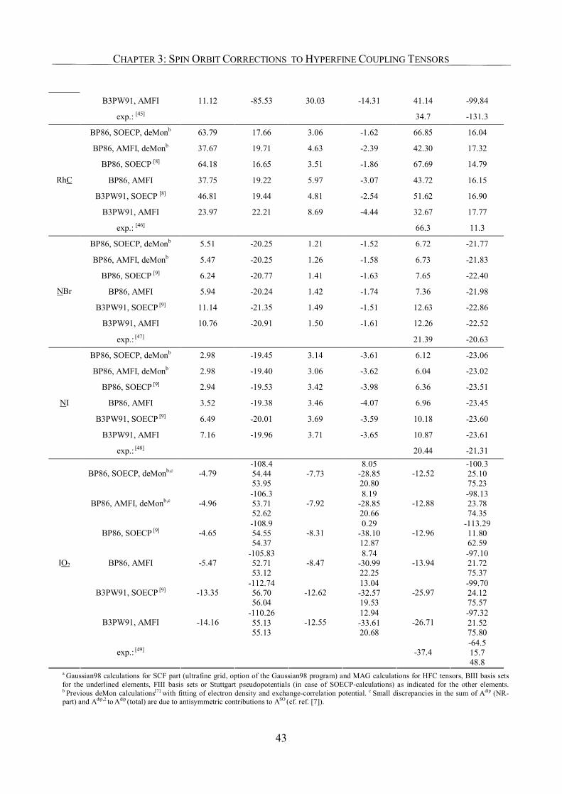
CHAPTER 3: SPIN ORBIT CORRECTIONS TO HYPERFINE COUPLING TENSORS
43
B3PW91, AMFI 11.12 -85.53 30.03 -14.31 41.14 -99.84
exp.: [45] 34.7 -131.3
BP86, SOECP, deMonb 63.79 17.66 3.06 -1.62 66.85 16.04
BP86, AMFI, deMonb 37.67 19.71 4.63 -2.39 42.30 17.32
BP86, SOECP [8] 64.18 16.65 3.51 -1.86 67.69 14.79
BP86, AMFI 37.75 19.22 5.97 -3.07 43.72 16.15
B3PW91, SOECP [8] 46.81 19.44 4.81 -2.54 51.62 16.90
B3PW91, AMFI 23.97 22.21 8.69 -4.44 32.67 17.77
RhC
exp.: [46] 66.3 11.3
BP86, SOECP, deMonb 5.51 -20.25 1.21 -1.52 6.72 -21.77
BP86, AMFI, deMonb 5.47 -20.25 1.26 -1.58 6.73 -21.83
BP86, SOECP [9] 6.24 -20.77 1.41 -1.63 7.65 -22.40
BP86, AMFI 5.94 -20.24 1.42 -1.74 7.36 -21.98
B3PW91, SOECP [9] 11.14 -21.35 1.49 -1.51 12.63 -22.86
B3PW91, AMFI 10.76 -20.91 1.50 -1.61 12.26 -22.52
NBr
exp.: [47] 21.39 -20.63
BP86, SOECP, deMonb 2.98 -19.45 3.14 -3.61 6.12 -23.06
BP86, AMFI, deMonb 2.98 -19.40 3.06 -3.62 6.04 -23.02
BP86, SOECP [9] 2.94 -19.53 3.42 -3.98 6.36 -23.51
BP86, AMFI 3.52 -19.38 3.46 -4.07 6.96 -23.45
B3PW91, SOECP [9] 6.49 -20.01 3.69 -3.59 10.18 -23.60
B3PW91, AMFI 7.16 -19.96 3.71 -3.65 10.87 -23.61
NI
exp.: [48] 20.44 -21.31
BP86, SOECP, deMonb,c -4.79 -108.4 54.44 53.95
-7.73 8.05
-28.85 20.80
-12.52 -100.3 25.10 75.23
BP86, AMFI, deMonb,c -4.96 -106.3 53.71 52.62
-7.92 8.19
-28.85 20.66
-12.88 -98.13 23.78 74.35
BP86, SOECP [9] -4.65 -108.9 54.55 54.37
-8.31 0.29
-38.10 12.87
-12.96 -113.29 11.80 62.59
BP86, AMFI -5.47 -105.83 52.71 53.12
-8.47 8.74
-30.99 22.25
-13.94 -97.10 21.72 75.37
B3PW91, SOECP [9] -13.35 -112.74 56.70 56.04
-12.62 13.04 -32.57 19.53
-25.97 -99.70 24.12 75.57
B3PW91, AMFI -14.16 -110.26 55.13 55.13
-12.55 12.94 -33.61 20.68
-26.71 -97.32 21.52 75.80
IO2
exp.: [49] -37.4 -64.5 15.7 48.8
a Gaussian98 calculations for SCF part (ultrafine grid, option of the Gaussian98 program) and MAG calculations for HFC tensors, BIII basis sets for the underlined elements, FIII basis sets or Stuttgart pseudopotentials (in case of SOECP-calculations) as indicated for the other elements. b Previous deMon calculations[7] with fitting of electron density and exchange-correlation potential. c Small discrepancies in the sum of Adip (NR-part) and Adip,2 to Adip (total) are due to antisymmetric contributions to ASO (cf. ref. [7]).
CHAPTER 3: SPIN ORBIT CORRECTIONS TO HYPERFINE COUPLING TENSORS
44
3.4 Conclusions
Spin-orbit (SO) corrections to metal hyperfine
coupling tensors may be significant already for
3d metal complexes, as amply confirmed by
results for the series of copper complexes inves-
tigated. In these cases, the addition of SO correc-
tions brings computed and experimental HFC
tensors into excellent agreement (at the B3PW91
hybrid DFT level). DFT combined with second-
order perturbation theory provides an efficient
and adequate tool to include SO effects into HFC
tensor calculations, provided the SO corrections
are not too large for a perturbation theoretical
treatment. In particular, a treatment with an unre-
stricted Kohn-Sham state and perturbational in-
clusion of spin-orbit coupling is well-suited to
include spin polarization straightforwardly.
The great advantage of the present implemen-
tation over alternative ones[4, 6, 24] is the use of
accurate and efficient non-empirical approxima-
tions to the microscopic SO Hamiltonian. This
allows a flexible and reliable treatment through-
out the Periodic Table and for very different
bonding situations, whereas semi-empirical SO
operators may be accurate in some cases but
difficult to parameterize in others. SO-ECPs on
heavy atoms offer a convenient way of including
also heavy-atom scalar relativistic effects in va-
lence-only calculations when dealing with the
HFC tensors of light nuclei in the neighborhood
of these heavy atoms.
In the case of transition metal complexes, we
confirm Neese’s observation that hybrid func-
tionals tend to enhance the SO contributions and
lead to improved agreement with experiment
compared to GGA functionals. One should em-
phasize, however, that care has to be taken in
cases where exact-exchange admixture leads to
appreciable spin contamination.[24] The presented
results for main-group diatomics allow no gen-
eral statement to be made with respect to supe-
rior performance of one or the other type of func-
tionals.
.
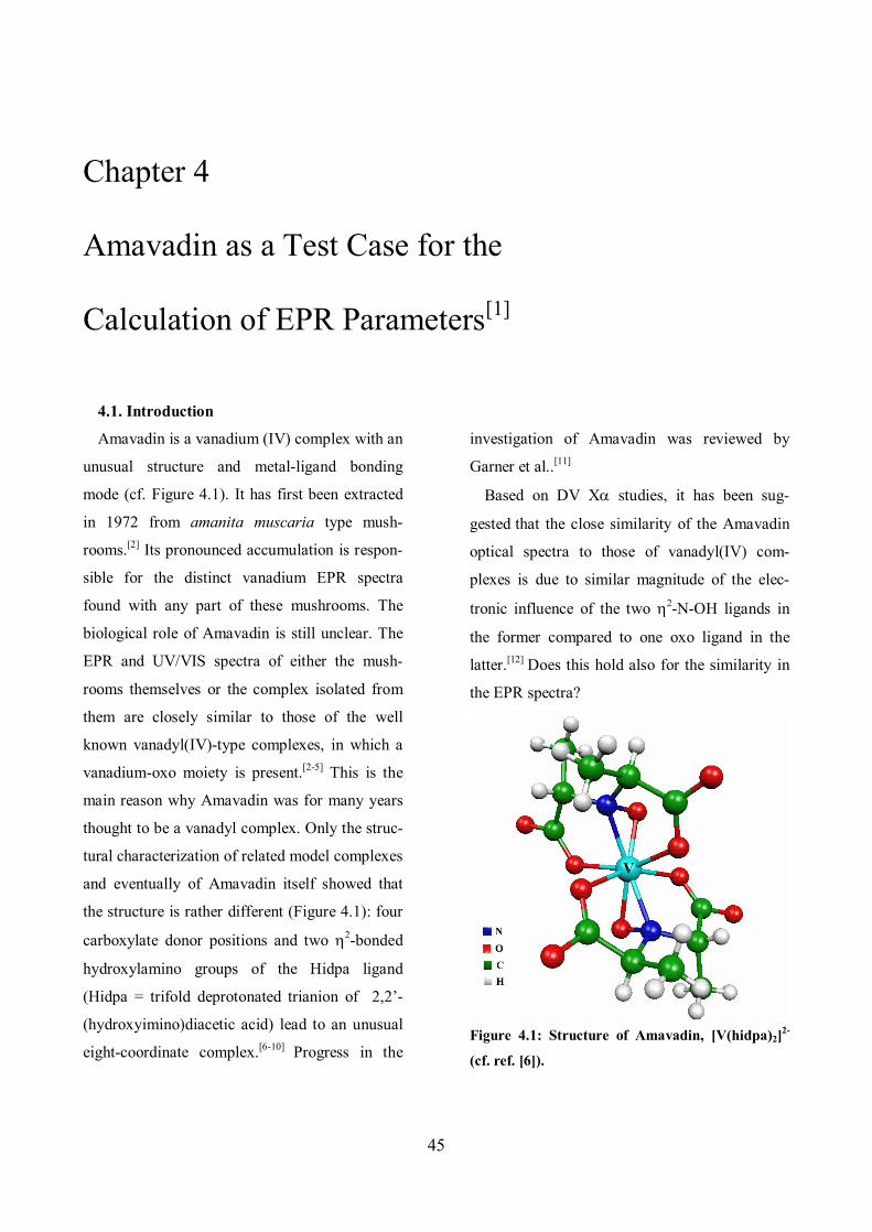
45
Chapter 4
Amavadin as a Test Case for the
Calculation of EPR Parameters[1]
4.1. Introduction
Amavadin is a vanadium (IV) complex with an
unusual structure and metal-ligand bonding
mode (cf. Figure 4.1). It has first been extracted
in 1972 from amanita muscaria type mush-
rooms.[2] Its pronounced accumulation is respon-
sible for the distinct vanadium EPR spectra
found with any part of these mushrooms. The
biological role of Amavadin is still unclear. The
EPR and UV/VIS spectra of either the mush-
rooms themselves or the complex isolated from
them are closely similar to those of the well
known vanadyl(IV)-type complexes, in which a
vanadium-oxo moiety is present.[2-5] This is the
main reason why Amavadin was for many years
thought to be a vanadyl complex. Only the struc-
tural characterization of related model complexes
and eventually of Amavadin itself showed that
the structure is rather different (Figure 4.1): four
carboxylate donor positions and two η2-bonded
hydroxylamino groups of the Hidpa ligand
(Hidpa = trifold deprotonated trianion of 2,2’-
(hydroxyimino)diacetic acid) lead to an unusual
eight-coordinate complex.[6-10] Progress in the
investigation of Amavadin was reviewed by
Garner et al..[11]
Based on DV Xα studies, it has been sug-
gested that the close similarity of the Amavadin
optical spectra to those of vanadyl(IV) com-
plexes is due to similar magnitude of the elec-
tronic influence of the two η2-N-OH ligands in
the former compared to one oxo ligand in the
latter.[12] Does this hold also for the similarity in
the EPR spectra?
Figure 4.1: Structure of Amavadin, [V(hidpa)2]2-
(cf. ref. [6]).
CHAPTER 4: AMAVADIN AS A TEST CASE FOR THE CALCULATION OF EPR PARAMETERS
46
Here we take Amavadin as an interesting test
case (a) to judge the performance of different
DFT methods for both hyperfine coupling- and
g-tensors, (b) to estimate the importance of spin-
orbit coupling effects even for the HFCC of a
relatively light metal like vanadium, (c) to ana-
lyze in detail the orientation of the two tensors,
and (d) to understand better the similarity of the
Amavadin EPR parameters to those of vanadyl
complexes (DFT studies of EPR parameters of
vanadyl(IV)[13, 14] and vanadocene(IV)[15] systems
have been carried out previously).
4.2. Computational Details
In the present work, the unrestricted Kohn-
Sham orbitals have been obtained with the Gaus-
sian98 program[16] and were transferred to the
MAG-ReSpect property package[17] by suitable
interface routines. The following exchange-
correlation functionals were compared: a) The
local density approximation in form of the
Vosko-Wilk-Nusair functional (VWN,[18] corre-
sponding to the VWN5 keyword in the Gaus-
sian98 code); b) the BP86 GGA functional;[19, 20]
c) the B3PW91 hybrid functional,[21-23] incorpo-
rating 20% HF exchange; d) user-defined one-
parameter BPW91-based hybrid functionals (op-
tion of the Gaussian 98 program and in the same
way taken for the MAG-ReSpect calculations) of
the general form:
88 91(1 ) ,HF B PWX X Ca E a E E+ − + (4-1)
with a (indicating the amount of Hartree-Fock
exchange) chosen as 0.35, 0.5 and 0.6, in the
following denoted as BPW91-35, BPW91-50 and
BPW91-60.
The efficient and accurate atomic mean-field
approximation (AMFI)[24, 25] has been used to
compute the matrix elements of the spin-orbit
operator. In g-tensor calculations, we employed a
common gauge at the transition metal nucleus.
The (15s11p6d)/[9s7p4d] metal basis set em-
ployed in our previous studies[26, 27] has been
used. DZVP basis sets[28] were used for the main
group atoms, without polarization p-functions for
hydrogen. The experimental structure of
Amavadin (crystallized with Ca2+ as counterion,
see ref. [6]) was used for calculations on the
dianion. Structures optimized by Saladino and
Larsen[14] were employed for VO(gly)2 and
VO(H2O)52+ .
4.3. Results and Discussion
A number of experimental EPR spectra are
available for comparison, both for Amavadin
itself,[4, 5] and for the smaller model complex
Ca[Ti(V)(hida)2](H2O)6.[3] These different spec-
tra are similar but do not coincide. For example,
the older spectra of Amavadin[4, 5] were analyzed
as an axial spectrum, whereas the spectrum of
McInnes et al. for the smaller model complex[3]
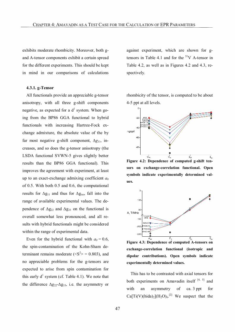
CHAPTER 4: AMAVADIN AS A TEST CASE FOR THE CALCULATION OF EPR PARAMETERS
47
exhibits moderate rhombicity. Moreover, both g-
and A-tensor components exhibit a certain spread
for the different experiments. This should be kept
in mind in our comparisons of calculations
against experiment, which are shown for g-
tensors in Table 4.1 and for the 51V A-tensor in
Table 4.2, as well as in Figures 4.2 and 4.3, re-
spectively.
4.3.1. g-Tensor
All functionals provide an appreciable g-tensor
anisotropy, with all three g-shift components
negative, as expected for a d1 system. When go-
ing from the BP86 GGA functional to hybrid
functionals with increasing Hartree-Fock ex-
change admixture, the absolute value of the by
far most negative g-shift component, ∆g11, in-
creases, and so does the g-tensor anisotropy (the
LSDA functional SVWN-5 gives slightly better
results than the BP86 GGA functional). This
improves the agreement with experiment, at least
up to an exact-exchange admixing coefficient a0
of 0.5. With both 0.5 and 0.6, the computational
results for ∆g11 and thus for ∆giso, fall into the
range of available experimental values. The de-
pendence of ∆g22 and ∆g33 on the functional is
overall somewhat less pronounced, and all re-
sults with hybrid functionals might be considered
within the range of experimental data.
Even for the hybrid functional with a0 = 0.6,
the spin-contamination of the Kohn-Sham de-
terminant remains moderate (<S2> = 0.803), and
no appreciable problems for the g-tensors are
expected to arise from spin contamination for
this early d1 system (cf. Table 4.1). We note that
the difference ∆g22-∆g33, i.e. the asymmetry or
rhombicity of the tensor, is computed to be about
4-5 ppt at all levels.
Figure 4.2: Dependence of computed g-shift ten-
sors on exchange-correlation functional. Open
symbols indicate experimentally determined val-
ues.
Figure 4.3: Dependence of computed A-tensors on
exchange-correlation functional (isotropic and
dipolar contributions). Open symbols indicate
experimentally determined values.
This has to be contrasted with axial tensors for
both experiments on Amavadin itself [4, 5] and
with an asymmetry of ca. 3 ppt for
Ca[Ti(V)(hida)2](H2O)6.[2] We suspect that the
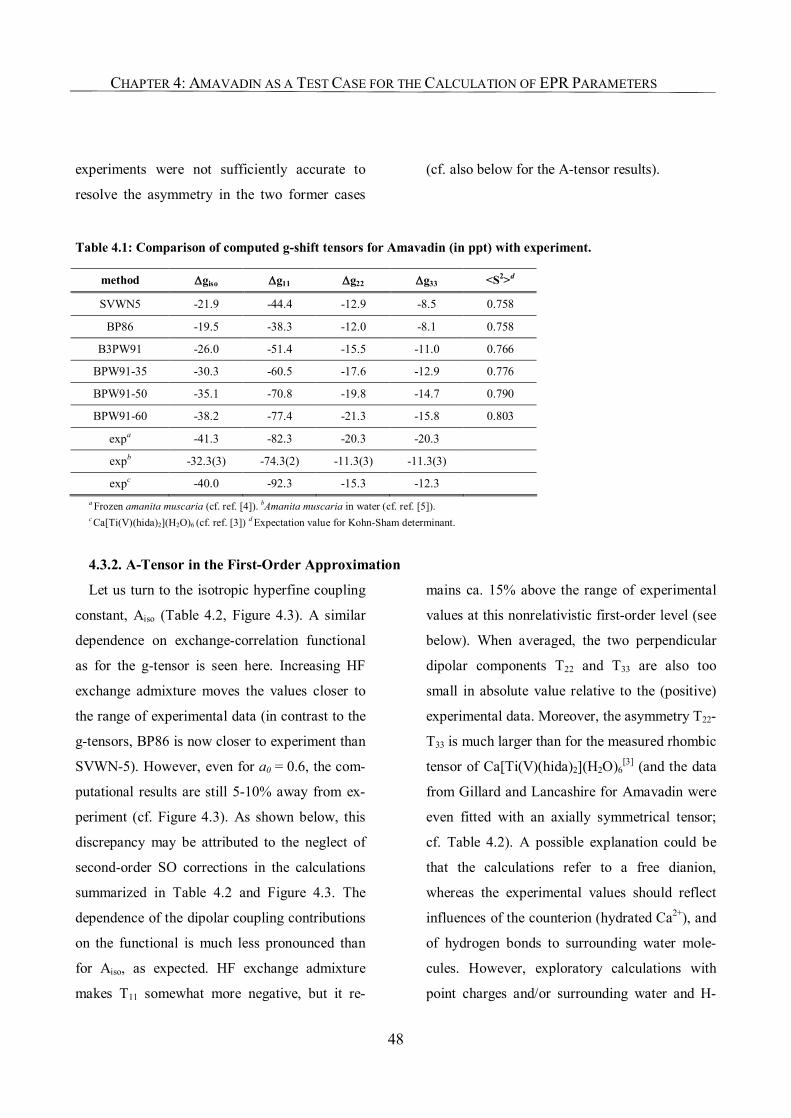
CHAPTER 4: AMAVADIN AS A TEST CASE FOR THE CALCULATION OF EPR PARAMETERS
48
experiments were not sufficiently accurate to
resolve the asymmetry in the two former cases
(cf. also below for the A-tensor results).
Table 4.1: Comparison of computed g-shift tensors for Amavadin (in ppt) with experiment.
method ∆giso ∆g11 ∆g22 ∆g33 <S2>d
SVWN5 -21.9 -44.4 -12.9 -8.5 0.758
BP86 -19.5 -38.3 -12.0 -8.1 0.758
B3PW91 -26.0 -51.4 -15.5 -11.0 0.766
BPW91-35 -30.3 -60.5 -17.6 -12.9 0.776
BPW91-50 -35.1 -70.8 -19.8 -14.7 0.790
BPW91-60 -38.2 -77.4 -21.3 -15.8 0.803
expa -41.3 -82.3 -20.3 -20.3
expb -32.3(3) -74.3(2) -11.3(3) -11.3(3)
expc -40.0 -92.3 -15.3 -12.3 a Frozen amanita muscaria (cf. ref. [4]). bAmanita muscaria in water (cf. ref. [5]). c Ca[Ti(V)(hida)2](H2O)6 (cf. ref. [3]) d Expectation value for Kohn-Sham determinant.
4.3.2. A-Tensor in the First-Order Approximation
Let us turn to the isotropic hyperfine coupling
constant, Aiso (Table 4.2, Figure 4.3). A similar
dependence on exchange-correlation functional
as for the g-tensor is seen here. Increasing HF
exchange admixture moves the values closer to
the range of experimental data (in contrast to the
g-tensors, BP86 is now closer to experiment than
SVWN-5). However, even for a0 = 0.6, the com-
putational results are still 5-10% away from ex-
periment (cf. Figure 4.3). As shown below, this
discrepancy may be attributed to the neglect of
second-order SO corrections in the calculations
summarized in Table 4.2 and Figure 4.3. The
dependence of the dipolar coupling contributions
on the functional is much less pronounced than
for Aiso, as expected. HF exchange admixture
makes T11 somewhat more negative, but it re-
mains ca. 15% above the range of experimental
values at this nonrelativistic first-order level (see
below). When averaged, the two perpendicular
dipolar components T22 and T33 are also too
small in absolute value relative to the (positive)
experimental data. Moreover, the asymmetry T22-
T33 is much larger than for the measured rhombic
tensor of Ca[Ti(V)(hida)2](H2O)6[3] (and the data
from Gillard and Lancashire for Amavadin were
even fitted with an axially symmetrical tensor;
cf. Table 4.2). A possible explanation could be
that the calculations refer to a free dianion,
whereas the experimental values should reflect
influences of the counterion (hydrated Ca2+), and
of hydrogen bonds to surrounding water mole-
cules. However, exploratory calculations with
point charges and/or surrounding water and H-
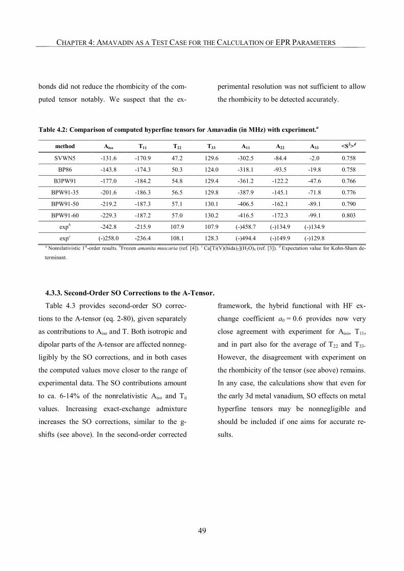
CHAPTER 4: AMAVADIN AS A TEST CASE FOR THE CALCULATION OF EPR PARAMETERS
49
bonds did not reduce the rhombicity of the com-
puted tensor notably. We suspect that the ex-
perimental resolution was not sufficient to allow
the rhombicity to be detected accurately.
Table 4.2: Comparison of computed hyperfine tensors for Amavadin (in MHz) with experiment.a
method Aiso T11 T22 T33 A11 A22 A33 <S2>d
SVWN5 -131.6 -170.9 47.2 129.6 -302.5 -84.4 -2.0 0.758
BP86 -143.8 -174.3 50.3 124.0 -318.1 -93.5 -19.8 0.758
B3PW91 -177.0 -184.2 54.8 129.4 -361.2 -122.2 -47.6 0.766
BPW91-35 -201.6 -186.3 56.5 129.8 -387.9 -145.1 -71.8 0.776
BPW91-50 -219.2 -187.3 57.1 130.1 -406.5 -162.1 -89.1 0.790
BPW91-60 -229.3 -187.2 57.0 130.2 -416.5 -172.3 -99.1 0.803
expb -242.8 -215.9 107.9 107.9 (-)458.7 (-)134.9 (-)134.9
expc (-)258.0 -236.4 108.1 128.3 (-)494.4 (-)149.9 (-)129.8 a Nonrelativistic 1st-order results. bFrozen amanita muscaria (ref. [4]). c Ca[Ti(V)(hida)2](H2O)6 (ref. [3]). d Expectation value for Kohn-Sham de-
terminant.
4.3.3. Second-Order SO Corrections to the A-Tensor.
Table 4.3 provides second-order SO correc-
tions to the A-tensor (eq. 2-80), given separately
as contributions to Aiso and T. Both isotropic and
dipolar parts of the A-tensor are affected nonneg-
ligibly by the SO corrections, and in both cases
the computed values move closer to the range of
experimental data. The SO contributions amount
to ca. 6-14% of the nonrelativistic Aiso and Tii
values. Increasing exact-exchange admixture
increases the SO corrections, similar to the g-
shifts (see above). In the second-order corrected
framework, the hybrid functional with HF ex-
change coefficient a0 = 0.6 provides now very
close agreement with experiment for Aiso, T11,
and in part also for the average of T22 and T33.
However, the disagreement with experiment on
the rhombicity of the tensor (see above) remains.
In any case, the calculations show that even for
the early 3d metal vanadium, SO effects on metal
hyperfine tensors may be nonnegligible and
should be included if one aims for accurate re-
sults.
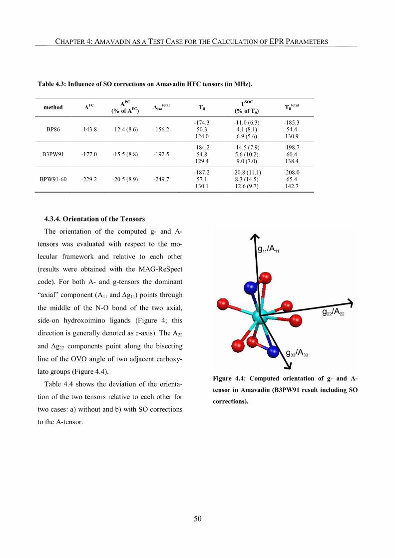
CHAPTER 4: AMAVADIN AS A TEST CASE FOR THE CALCULATION OF EPR PARAMETERS
50
Table 4.3: Influence of SO corrections on Amavadin HFC tensors (in MHz).
method AFC APC
(% of AFC) Aisototal Tii
TSOC
(% of Tii) Tii
total
BP86 -143.8 -12.4 (8.6) -156.2 -174.3 50.3 124.0
-11.0 (6.3) 4.1 (8.1) 6.9 (5.6)
-185.3 54.4 130.9
B3PW91 -177.0 -15.5 (8.8) -192.5 -184.2 54.8 129.4
-14.5 (7.9) 5.6 (10.2) 9.0 (7.0)
-198.7 60.4 138.4
BPW91-60 -229.2 -20.5 (8.9) -249.7 -187.2 57.1 130.1
-20.8 (11.1) 8.3 (14.5) 12.6 (9.7)
-208.0 65.4 142.7
4.3.4. Orientation of the Tensors
The orientation of the computed g- and A-
tensors was evaluated with respect to the mo-
lecular framework and relative to each other
(results were obtained with the MAG-ReSpect
code). For both A- and g-tensors the dominant
“axial” component (A11 and ∆g11) points through
the middle of the N-O bond of the two axial,
side-on hydroxoimino ligands (Figure 4; this
direction is generally denoted as z-axis). The A22
and ∆g22 components point along the bisecting
line of the OVO angle of two adjacent carboxy-
lato groups (Figure 4.4).
Table 4.4 shows the deviation of the orienta-
tion of the two tensors relative to each other for
two cases: a) without and b) with SO corrections
to the A-tensor.
Figure 4.4: Computed orientation of g- and A-
tensor in Amavadin (B3PW91 result including SO
corrections).
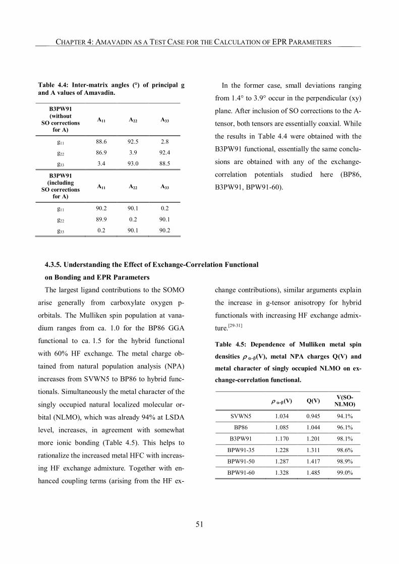
CHAPTER 4: AMAVADIN AS A TEST CASE FOR THE CALCULATION OF EPR PARAMETERS
51
Table 4.4: Inter-matrix angles (°) of principal g and A values of Amavadin.
B3PW91 (without
SO corrections for A)
A11 A22 A33
g11 88.6 92.5 2.8
g22 86.9 3.9 92.4
g33 3.4 93.0 88.5
B3PW91 (including
SO corrections for A)
A11 A22 A33
g11 90.2 90.1 0.2
g22 89.9 0.2 90.1
g33 0.2 90.1 90.2
In the former case, small deviations ranging
from 1.4° to 3.9° occur in the perpendicular (xy)
plane. After inclusion of SO corrections to the A-
tensor, both tensors are essentially coaxial. While
the results in Table 4.4 were obtained with the
B3PW91 functional, essentially the same conclu-
sions are obtained with any of the exchange-
correlation potentials studied here (BP86,
B3PW91, BPW91-60).
4.3.5. Understanding the Effect of Exchange-Correlation Functional
on Bonding and EPR Parameters
The largest ligand contributions to the SOMO
arise generally from carboxylate oxygen p-
orbitals. The Mulliken spin population at vana-
dium ranges from ca. 1.0 for the BP86 GGA
functional to ca. 1.5 for the hybrid functional
with 60% HF exchange. The metal charge ob-
tained from natural population analysis (NPA)
increases from SVWN5 to BP86 to hybrid func-
tionals. Simultaneously the metal character of the
singly occupied natural localized molecular or-
bital (NLMO), which was already 94% at LSDA
level, increases, in agreement with somewhat
more ionic bonding (Table 4.5). This helps to
rationalize the increased metal HFC with increas-
ing HF exchange admixture. Together with en-
hanced coupling terms (arising from the HF ex-
change contributions), similar arguments explain
the increase in g-tensor anisotropy for hybrid
functionals with increasing HF exchange admix-
ture.[29-31]
Table 4.5: Dependence of Mulliken metal spin
densities ρ α−β(V), metal NPA charges Q(V) and
metal character of singly occupied NLMO on ex-
change-correlation functional.
ρ α−β(V) Q(V) V(SO-NLMO)
SVWN5 1.034 0.945 94.1%
BP86 1.085 1.044 96.1%
B3PW91 1.170 1.201 98.1%
BPW91-35 1.228 1.311 98.6%
BPW91-50 1.287 1.417 98.9%
BPW91-60 1.328 1.485 99.0%
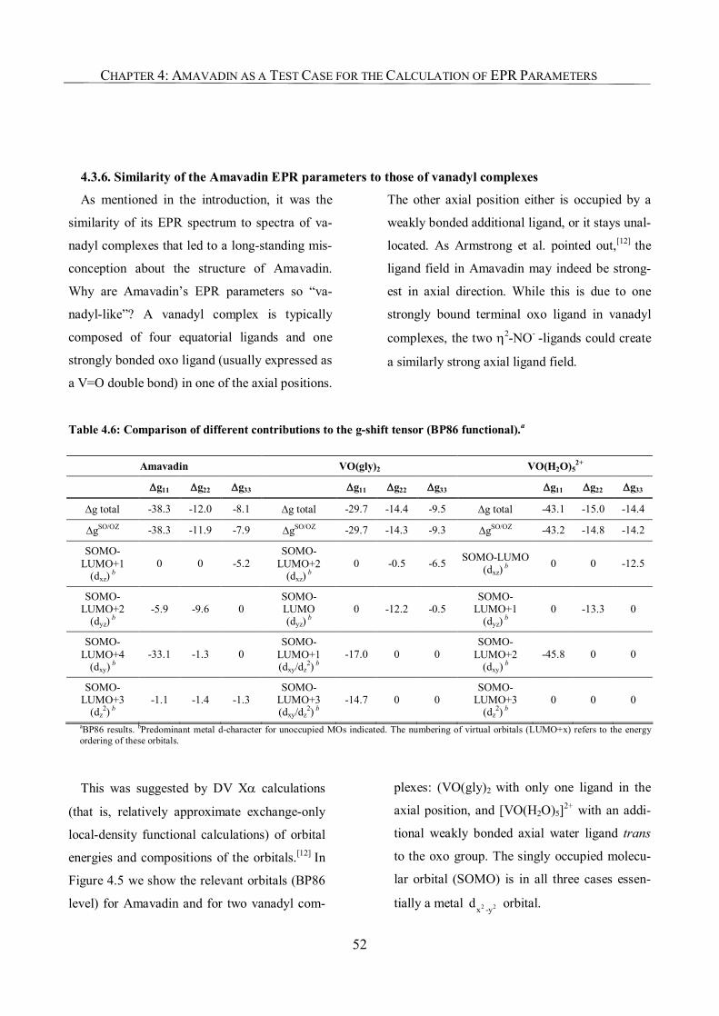
CHAPTER 4: AMAVADIN AS A TEST CASE FOR THE CALCULATION OF EPR PARAMETERS
52
4.3.6. Similarity of the Amavadin EPR parameters to those of vanadyl complexes
As mentioned in the introduction, it was the
similarity of its EPR spectrum to spectra of va-
nadyl complexes that led to a long-standing mis-
conception about the structure of Amavadin.
Why are Amavadin’s EPR parameters so “va-
nadyl-like”? A vanadyl complex is typically
composed of four equatorial ligands and one
strongly bonded oxo ligand (usually expressed as
a V=O double bond) in one of the axial positions.
The other axial position either is occupied by a
weakly bonded additional ligand, or it stays unal-
located. As Armstrong et al. pointed out,[12] the
ligand field in Amavadin may indeed be strong-
est in axial direction. While this is due to one
strongly bound terminal oxo ligand in vanadyl
complexes, the two η2-NO- -ligands could create
a similarly strong axial ligand field.
Table 4.6: Comparison of different contributions to the g-shift tensor (BP86 functional).a
Amavadin VO(gly)2 VO(H2O)52+
∆g11 ∆g22 ∆g33 ∆g11 ∆g22 ∆g33 ∆g11 ∆g22 ∆g33
∆g total -38.3 -12.0 -8.1 ∆g total -29.7 -14.4 -9.5 ∆g total -43.1 -15.0 -14.4
∆gSO/OZ -38.3 -11.9 -7.9 ∆gSO/OZ -29.7 -14.3 -9.3 ∆gSO/OZ -43.2 -14.8 -14.2
SOMO-LUMO+1
(dxz) b 0 0 -5.2
SOMO-LUMO+2
(dxz) b 0 -0.5 -6.5 SOMO-LUMO
(dxz) b 0 0 -12.5
SOMO-LUMO+2
(dyz) b -5.9 -9.6 0
SOMO- LUMO (dyz) b
0 -12.2 -0.5 SOMO-
LUMO+1 (dyz) b
0 -13.3 0
SOMO-LUMO+4
(dxy) b -33.1 -1.3 0
SOMO-LUMO+1 (dxy/dz
2) b -17.0 0 0
SOMO-LUMO+2
(dxy) b -45.8 0 0
SOMO-LUMO+3
(dz2) b
-1.1 -1.4 -1.3 SOMO-
LUMO+3 (dxy/dz
2) b -14.7 0 0
SOMO-LUMO+3
(dz2) b
0 0 0
aBP86 results. bPredominant metal d-character for unoccupied MOs indicated. The numbering of virtual orbitals (LUMO+x) refers to the energy ordering of these orbitals.
This was suggested by DV Xα calculations
(that is, relatively approximate exchange-only
local-density functional calculations) of orbital
energies and compositions of the orbitals.[12] In
Figure 4.5 we show the relevant orbitals (BP86
level) for Amavadin and for two vanadyl com-
plexes: (VO(gly)2 with only one ligand in the
axial position, and [VO(H2O)5]2+ with an addi-
tional weakly bonded axial water ligand trans
to the oxo group. The singly occupied molecu-
lar orbital (SOMO) is in all three cases essen-
tially a metal 2 2x -yd orbital.
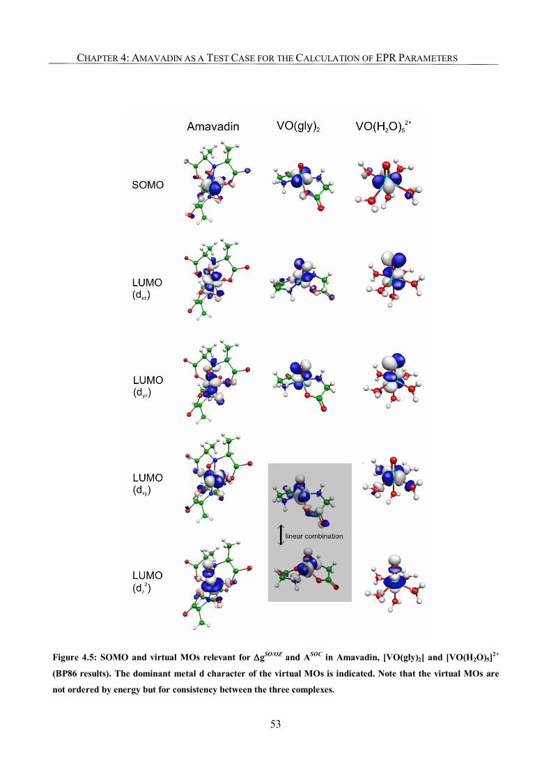
CHAPTER 4: AMAVADIN AS A TEST CASE FOR THE CALCULATION OF EPR PARAMETERS
53
Figure 4.5: SOMO and virtual MOs relevant for ∆gSO/OZ and ASOC in Amavadin, [VO(gly)2] and [VO(H2O)5]2+
(BP86 results). The dominant metal d character of the virtual MOs is indicated. Note that the virtual MOs are
not ordered by energy but for consistency between the three complexes.
CHAPTER 4: AMAVADIN AS A TEST CASE FOR THE CALCULATION OF EPR PARAMETERS
54
In agreement with textbook knowledge on d1
systems with 2 2x -yd SOMO,[32, 33] this explains at
once the similarity of the HFC tensors for 51V:
the most negative A-tensor component has to
point roughly in axial z-direction (the SO contri-
butions are also largest in this direction, see be-
low). The second-order ∆gSO/OZ term dominates
the ∆g-tensor (eq. 2-71). Analyses of ∆gSO/OZ in
terms of contributions from specific orbital inter-
actions have been compared for Amavadin,
VO(gly)2, and [VO(H2O)5]2+ (Table 4.6). The
main contribution to the most negative ∆g11-
component (oriented in z-direction) arises from
magnetic coupling of the SOMO with the lowest
unoccupied molecular orbital (LUMO), which
has essentially dxy–character (Figure 4.5;
VO(gly)2 does not exhibit a “pure” dxy-type
LUMO but two orbitals that are linear combina-
tions with dxy and dz2 character). The same cou-
pling dominates the largest component of the
second-order corrections to the HFC tensor (eq.
2-79). The less pronounced equatorial ∆gSO/OZ-
components arise mainly from couplings of the
SOMO to unoccupied orbitals of dxz- and dyz-
character (Figure 4.5, Table 4.6). In all three
cases magnetic couplings between other orbitals
are small (less than ±1 ppt) and are therefore not
shown in Table 4.6.
4.4. Conclusions
Amavadin is a structurally fascinating vana-
dium complex whose biological role in mush-
rooms is still a matter of study. Here the EPR
parameters of Amavadin have been analyzed in
detail, and we used the complex to evaluate DFT
methods for the computation of EPR parameters
in transition metal complexes. In particular, the
influence of increasing amounts of Hartree-Fock
exchange in hybrid functionals on both g- and A-
tensors was evaluated. Even up to 60% exact-
exchange admixture, agreement with experiment
is still improved with nonlocal hybrid potentials.
This is due to improved descriptions of metal-
ligand bond ionicity (for both g- and A-tensors47)
and enhanced metal core-shell spin polarization
(for A-tensors20). Due to the mainly nonbonding
nature of the SOMO,20 spin contamination of the
Kohn-Sham determinant is not a problem for this
early d1 complex.
Second-order spin-orbit corrections account
for ca. 6-10% of the computed isotropic and di-
polar metal hyperfine tensor components and
thus are clearly nonnegligible in accurate calcu-
lations of this EPR parameter for Amavadin (the
same holds for the related vanadyl complexes).
While the g- and A-tensors deviate very slightly
from covariance when the A-tensor is computed
nonrelativistically, the second-order SO correc-
tions make the two tensors almost coincide. Both
tensors are strongly dominated by the axial direc-
tion given by the two η2-NO- -ligands. This arises
from the strong ligand field of these two groups,
and from the resulting metal 2 2x -yd -character of
the SOMO. A similar character of the frontier
CHAPTER 4: AMAVADIN AS A TEST CASE FOR THE CALCULATION OF EPR PARAMETERS
55
orbitals in turn explains the close similarity of
the EPR parameters of Amavadin to those of
vanadyl complexes, which has kept the structure
of this interesting biological complex in the dark
for such a long time.

56
57
Chapter 5
EPR Parameters and Spin-Density Distributions of
Azurin and other Blue-Copper Proteins
5.1. Introduction
Blue copper proteins (or type I copper pro-
teins) are often considered the prototypical elec-
tron-transfer proteins. They are probably among
the metalloproteins studied most thoroughly by a
host of crystallographical, spectroscopical, and
theoretical methods.[1-9] One reason is their dis-
torted tetrahedral copper coordination, which has
been central to a still ongoing debate about the
role of an “entatic” or “rack” state for the func-
tion of metalloproteins.[10-12] Additionally, the
strong blue color, due to an intense excitation
near 600 nm, and a narrow 65Cu hyperfine cou-
pling of the oxidized CuII state are spectroscopic
characteristics that have attracted substantial
interest.[13, 14] The hyperfine coupling is related to
the mechanistically important question, how the
spin density is distributed between the metal and
the strongly bound equatorial cysteine ligand.
With the aim to establish the electronic struc-
ture and spin density of blue copper sites, par-
ticularly extended spectroscopic and theoretical
studies have been carried out on plastocyanin, by
Solomon and coworkers and by others.[15-17] This
included optical spectroscopies (including mag-
netic circular dichroism, MCD), X-ray absorp-
tion spectroscopies (XAS) at various frequencies,
variable-energy photoelectron spectroscopy
(VEPES), electron paramagnetic resonance
(EPR), and theoretical treatments ranging all the
way from early scattered-wave Xα and semiem-
pirical approaches to state-of-the-art density-
functional theory (DFT) methods, and even to
post-Hartree-Fock treatments for smaller model
systems. Combining the spectroscopic data with
various computations, Solomon et al. arrived at a
relatively large metal-ligand (Cu-S) covalency
and suggested this as the primary reason for the
small A|| copper hyperfine splitting and blue
color of blue copper proteins. Hybrid density
functional methods with about 38% exact-
exchange admixture were indicated to provide
the most reliable spin-density distribution. The
route along which these conclusions were ob-
tained is, however, a relatively indirect one:
Copper K-edge XAS was used to rule out an
earlier proposed 2 2 zx yd p
−− hybridization as
reason for the small copper A||. Approximate Xα-
SW calculations, an early version of DFT, were
CHAPTER 5: EPR PARAMETERS OF AZURIN AND BLUE-COPPER PROTEINS
58
used to estimate the EPR g-tensor. While they
confirmed the experimentally observed order of
g|| > g⊥ > ge, the g|| component and thus the g-
anisotropy were underestimated by the calcula-
tions. This was attributed to a too large metal-
ligand covalency in the calculations, associated
with too much delocalization of the spin density
onto the cysteine ligand. After reducing the muf-
fin-tin sphere sizes around copper arbitrarily, the
spin delocalization was reduced, and good
agreement with the experimental g-tensor was
obtained. The resulting spin-density distribution
(with slightly more spin on copper than on the
cysteine sulfur, and slight delocalization onto the
two histidine δ-N atoms) was considered ade-
quate. It was probed by various further spectro-
scopic techniques, including Cu L-edge XAS, S
K-edge XAS, and low-temperature MCD spec-
troscopy. The large Cu-S covalency was consid-
ered to constitute the most special feature of the
blue-copper proteins compared to more regular
copper thiolato complexes, explaining the special
spectroscopic characteristics. The obtained “ex-
perimental” spin density was used to calibrate
more recent computations using state-of-the-art
DFT approaches. The abovementioned hybrid
functional with 38% Hartree-Fock-exchange
admixture was the method judged most adequate
based on this procedure.
While the evidence provided by all of the ex-
periments and computations appears rather com-
pelling, and a relatively large Cu-S covalency is
certainly an important feature of the blue copper
proteins and their function, the reasoning is a
relatively indirect one. In view of the fundamen-
tal importance of the spin density for the function
of these electron-transfer proteins, and of the
sensitive dependence of the electronic structure
on the theoretical treatment, it would be more
satisfying to be able to compute the EPR parame-
ters of the system – as the most faithful probe of
the spin-density distribution – directly with state-
of-the-art quantum chemical methodology. No-
tably, such calculations should be able to recon-
cile the relatively large g-anisotropy (which
points to appreciable metal-centered spin) with
the small copper hyperfine coupling (which has
been taken to suggest relatively small metal spin
density).
In this paper, we provide such state-of-the-art
calculations of EPR parameters in blue-copper
proteins, and we study in particular the depend-
ence of the EPR parameters and spin density on
admixture of exact exchange in hybrid density
functionals. While computations will be pre-
sented for models of azurin, plastocyanin, and
stellacyanin (Figure 5.1), our main focus will be
on azurin: This is the blue copper protein studied
most thoroughly by multiple-frequency EPR, as
well as by electron-nuclear double resonance
(ENDOR) and electron-spin-echo-modulation
(ESEEM) spectroscopies, in particular by Gro-
enen and coworkers.[5-7, 18] DFT studies have
focused on hyperfine couplings, with rather lim-
ited accuracy. The g-tensor of azurin has even
been calculated by MRD-CI calculations, but
with a number of substantial approximations
involved (see discussion below).[19]
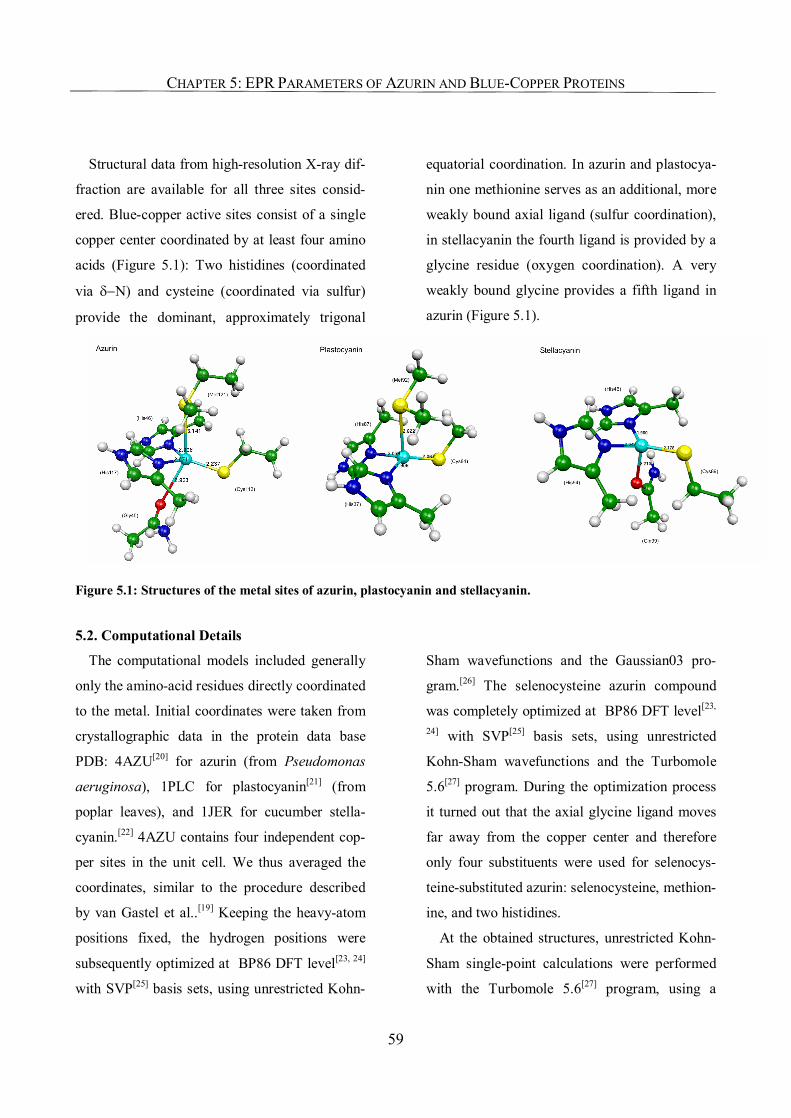
CHAPTER 5: EPR PARAMETERS OF AZURIN AND BLUE-COPPER PROTEINS
59
Structural data from high-resolution X-ray dif-
fraction are available for all three sites consid-
ered. Blue-copper active sites consist of a single
copper center coordinated by at least four amino
acids (Figure 5.1): Two histidines (coordinated
via δ−N) and cysteine (coordinated via sulfur)
provide the dominant, approximately trigonal
equatorial coordination. In azurin and plastocya-
nin one methionine serves as an additional, more
weakly bound axial ligand (sulfur coordination),
in stellacyanin the fourth ligand is provided by a
glycine residue (oxygen coordination). A very
weakly bound glycine provides a fifth ligand in
azurin (Figure 5.1).
Figure 5.1: Structures of the metal sites of azurin, plastocyanin and stellacyanin.
5.2. Computational Details
The computational models included generally
only the amino-acid residues directly coordinated
to the metal. Initial coordinates were taken from
crystallographic data in the protein data base
PDB: 4AZU[20] for azurin (from Pseudomonas
aeruginosa), 1PLC for plastocyanin[21] (from
poplar leaves), and 1JER for cucumber stella-
cyanin.[22] 4AZU contains four independent cop-
per sites in the unit cell. We thus averaged the
coordinates, similar to the procedure described
by van Gastel et al..[19] Keeping the heavy-atom
positions fixed, the hydrogen positions were
subsequently optimized at BP86 DFT level[23, 24]
with SVP[25] basis sets, using unrestricted Kohn-
Sham wavefunctions and the Gaussian03 pro-
gram.[26] The selenocysteine azurin compound
was completely optimized at BP86 DFT level[23,
24] with SVP[25] basis sets, using unrestricted
Kohn-Sham wavefunctions and the Turbomole
5.6[27] program. During the optimization process
it turned out that the axial glycine ligand moves
far away from the copper center and therefore
only four substituents were used for selenocys-
teine-substituted azurin: selenocysteine, methion-
ine, and two histidines.
At the obtained structures, unrestricted Kohn-
Sham single-point calculations were performed
with the Turbomole 5.6[27] program, using a
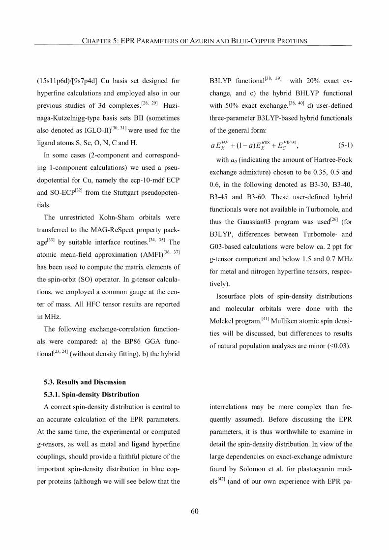
CHAPTER 5: EPR PARAMETERS OF AZURIN AND BLUE-COPPER PROTEINS
60
(15s11p6d)/[9s7p4d] Cu basis set designed for
hyperfine calculations and employed also in our
previous studies of 3d complexes.[28, 29] Huzi-
naga-Kutzelnigg-type basis sets BII (sometimes
also denoted as IGLO-II)[30, 31] were used for the
ligand atoms S, Se, O, N, C and H.
In some cases (2-component and correspond-
ing 1-component calculations) we used a pseu-
dopotential for Cu, namely the ecp-10-mdf ECP
and SO-ECP[32] from the Stuttgart pseudopoten-
tials.
The unrestricted Kohn-Sham orbitals were
transferred to the MAG-ReSpect property pack-
age[33] by suitable interface routines.[34, 35] The
atomic mean-field approximation (AMFI)[36, 37]
has been used to compute the matrix elements of
the spin-orbit (SO) operator. In g-tensor calcula-
tions, we employed a common gauge at the cen-
ter of mass. All HFC tensor results are reported
in MHz.
The following exchange-correlation function-
als were compared: a) the BP86 GGA func-
tional[23, 24] (without density fitting), b) the hybrid
B3LYP functional[38, 39] with 20% exact ex-
change, and c) the hybrid BHLYP functional
with 50% exact exchange.[38, 40] d) user-defined
three-parameter B3LYP-based hybrid functionals
of the general form: 88 91(1 ) ,HF B PW
X X Ca E a E E+ − + (5-1)
with a0 (indicating the amount of Hartree-Fock
exchange admixture) chosen to be 0.35, 0.5 and
0.6, in the following denoted as B3-30, B3-40,
B3-45 and B3-60. These user-defined hybrid
functionals were not available in Turbomole, and
thus the Gaussian03 program was used[26] (for
B3LYP, differences between Turbomole- and
G03-based calculations were below ca. 2 ppt for
g-tensor component and below 1.5 and 0.7 MHz
for metal and nitrogen hyperfine tensors, respec-
tively).
Isosurface plots of spin-density distributions
and molecular orbitals were done with the
Molekel program.[41] Mulliken atomic spin densi-
ties will be discussed, but differences to results
of natural population analyses are minor (<0.03).
5.3. Results and Discussion
5.3.1. Spin-density Distribution
A correct spin-density distribution is central to
an accurate calculation of the EPR parameters.
At the same time, the experimental or computed
g-tensors, as well as metal and ligand hyperfine
couplings, should provide a faithful picture of the
important spin-density distribution in blue cop-
per proteins (although we will see below that the
interrelations may be more complex than fre-
quently assumed). Before discussing the EPR
parameters, it is thus worthwhile to examine in
detail the spin-density distribution. In view of the
large dependencies on exact-exchange admixture
found by Solomon et al. for plastocyanin mod-
els[42] (and of our own experience with EPR pa-
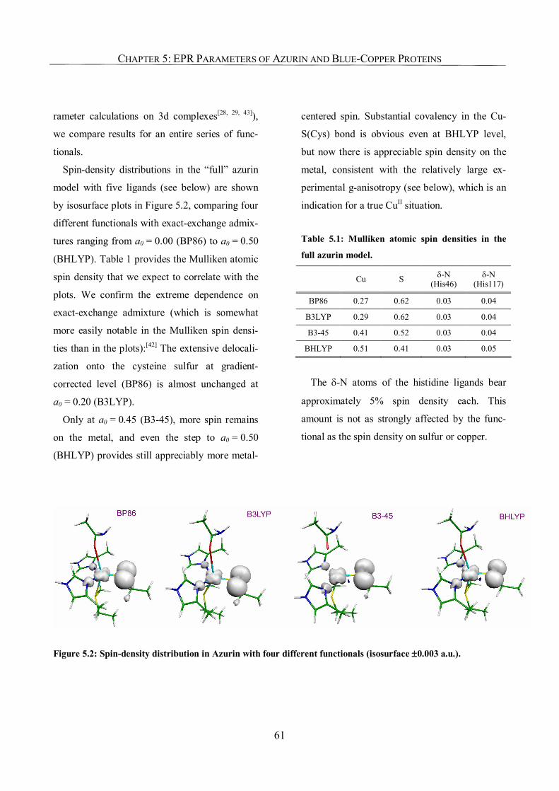
CHAPTER 5: EPR PARAMETERS OF AZURIN AND BLUE-COPPER PROTEINS
61
rameter calculations on 3d complexes[28, 29, 43]),
we compare results for an entire series of func-
tionals.
Spin-density distributions in the “full” azurin
model with five ligands (see below) are shown
by isosurface plots in Figure 5.2, comparing four
different functionals with exact-exchange admix-
tures ranging from a0 = 0.00 (BP86) to a0 = 0.50
(BHLYP). Table 1 provides the Mulliken atomic
spin density that we expect to correlate with the
plots. We confirm the extreme dependence on
exact-exchange admixture (which is somewhat
more easily notable in the Mulliken spin densi-
ties than in the plots):[42] The extensive delocali-
zation onto the cysteine sulfur at gradient-
corrected level (BP86) is almost unchanged at
a0 = 0.20 (B3LYP).
Only at a0 = 0.45 (B3-45), more spin remains
on the metal, and even the step to a0 = 0.50
(BHLYP) provides still appreciably more metal-
centered spin. Substantial covalency in the Cu-
S(Cys) bond is obvious even at BHLYP level,
but now there is appreciable spin density on the
metal, consistent with the relatively large ex-
perimental g-anisotropy (see below), which is an
indication for a true CuII situation.
Table 5.1: Mulliken atomic spin densities in the
full azurin model.
Cu S δ-N (His46)
δ-N (His117)
BP86 0.27 0.62 0.03 0.04
B3LYP 0.29 0.62 0.03 0.04
B3-45 0.41 0.52 0.03 0.04
BHLYP 0.51 0.41 0.03 0.05
The δ-N atoms of the histidine ligands bear
approximately 5% spin density each. This
amount is not as strongly affected by the func-
tional as the spin density on sulfur or copper.
Figure 5.2: Spin-density distribution in Azurin with four different functionals (isosurface ±0.003 a.u.).
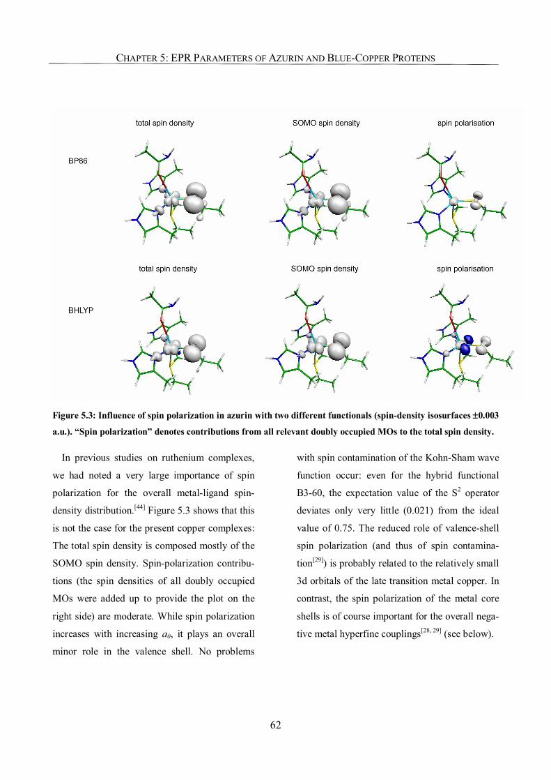
CHAPTER 5: EPR PARAMETERS OF AZURIN AND BLUE-COPPER PROTEINS
62
Figure 5.3: Influence of spin polarization in azurin with two different functionals (spin-density isosurfaces ±0.003
a.u.). “Spin polarization” denotes contributions from all relevant doubly occupied MOs to the total spin density.
In previous studies on ruthenium complexes,
we had noted a very large importance of spin
polarization for the overall metal-ligand spin-
density distribution.[44] Figure 5.3 shows that this
is not the case for the present copper complexes:
The total spin density is composed mostly of the
SOMO spin density. Spin-polarization contribu-
tions (the spin densities of all doubly occupied
MOs were added up to provide the plot on the
right side) are moderate. While spin polarization
increases with increasing a0, it plays an overall
minor role in the valence shell. No problems
with spin contamination of the Kohn-Sham wave
function occur: even for the hybrid functional
B3-60, the expectation value of the S2 operator
deviates only very little (0.021) from the ideal
value of 0.75. The reduced role of valence-shell
spin polarization (and thus of spin contamina-
tion[29]) is probably related to the relatively small
3d orbitals of the late transition metal copper. In
contrast, the spin polarization of the metal core
shells is of course important for the overall nega-
tive metal hyperfine couplings[28, 29] (see below).
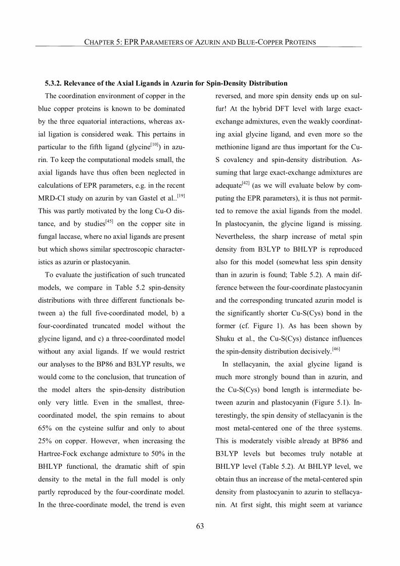
CHAPTER 5: EPR PARAMETERS OF AZURIN AND BLUE-COPPER PROTEINS
63
5.3.2. Relevance of the Axial Ligands in Azurin for Spin-Density Distribution
The coordination environment of copper in the
blue copper proteins is known to be dominated
by the three equatorial interactions, whereas ax-
ial ligation is considered weak. This pertains in
particular to the fifth ligand (glycine[10]) in azu-
rin. To keep the computational models small, the
axial ligands have thus often been neglected in
calculations of EPR parameters, e.g. in the recent
MRD-CI study on azurin by van Gastel et al..[19]
This was partly motivated by the long Cu-O dis-
tance, and by studies[45] on the copper site in
fungal laccase, where no axial ligands are present
but which shows similar spectroscopic character-
istics as azurin or plastocyanin.
To evaluate the justification of such truncated
models, we compare in Table 5.2 spin-density
distributions with three different functionals be-
tween a) the full five-coordinated model, b) a
four-coordinated truncated model without the
glycine ligand, and c) a three-coordinated model
without any axial ligands. If we would restrict
our analyses to the BP86 and B3LYP results, we
would come to the conclusion, that truncation of
the model alters the spin-density distribution
only very little. Even in the smallest, three-
coordinated model, the spin remains to about
65% on the cysteine sulfur and only to about
25% on copper. However, when increasing the
Hartree-Fock exchange admixture to 50% in the
BHLYP functional, the dramatic shift of spin
density to the metal in the full model is only
partly reproduced by the four-coordinate model.
In the three-coordinate model, the trend is even
reversed, and more spin density ends up on sul-
fur! At the hybrid DFT level with large exact-
exchange admixtures, even the weakly coordinat-
ing axial glycine ligand, and even more so the
methionine ligand are thus important for the Cu-
S covalency and spin-density distribution. As-
suming that large exact-exchange admixtures are
adequate[42] (as we will evaluate below by com-
puting the EPR parameters), it is thus not permit-
ted to remove the axial ligands from the model.
In plastocyanin, the glycine ligand is missing.
Nevertheless, the sharp increase of metal spin
density from B3LYP to BHLYP is reproduced
also for this model (somewhat less spin density
than in azurin is found; Table 5.2). A main dif-
ference between the four-coordinate plastocyanin
and the corresponding truncated azurin model is
the significantly shorter Cu-S(Cys) bond in the
former (cf. Figure 1). As has been shown by
Shuku et al., the Cu-S(Cys) distance influences
the spin-density distribution decisively.[46]
In stellacyanin, the axial glycine ligand is
much more strongly bound than in azurin, and
the Cu-S(Cys) bond length is intermediate be-
tween azurin and plastocyanin (Figure 5.1). In-
terestingly, the spin density of stellacyanin is the
most metal-centered one of the three systems.
This is moderately visible already at BP86 and
B3LYP levels but becomes truly notable at
BHLYP level (Table 5.2). At BHLYP level, we
obtain thus an increase of the metal-centered spin
density from plastocyanin to azurin to stellacya-
nin. At first sight, this might seem at variance
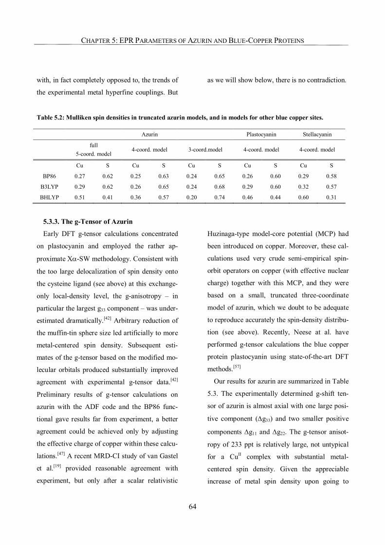
CHAPTER 5: EPR PARAMETERS OF AZURIN AND BLUE-COPPER PROTEINS
64
with, in fact completely opposed to, the trends of
the experimental metal hyperfine couplings. But
as we will show below, there is no contradiction.
Table 5.2: Mulliken spin densities in truncated azurin models, and in models for other blue copper sites.
Azurin Plastocyanin Stellacyanin
full
5-coord. model 4-coord. model 3-coord.model 4-coord. model 4-coord. model
Cu S Cu S Cu S Cu S Cu S
BP86 0.27 0.62 0.25 0.63 0.24 0.65 0.26 0.60 0.29 0.58
B3LYP 0.29 0.62 0.26 0.65 0.24 0.68 0.29 0.60 0.32 0.57
BHLYP 0.51 0.41 0.36 0.57 0.20 0.74 0.46 0.44 0.60 0.31
5.3.3. The g-Tensor of Azurin
Early DFT g-tensor calculations concentrated
on plastocyanin and employed the rather ap-
proximate Xα-SW methodology. Consistent with
the too large delocalization of spin density onto
the cysteine ligand (see above) at this exchange-
only local-density level, the g-anisotropy – in
particular the largest g33 component – was under-
estimated dramatically.[42] Arbitrary reduction of
the muffin-tin sphere size led artificially to more
metal-centered spin density. Subsequent esti-
mates of the g-tensor based on the modified mo-
lecular orbitals produced substantially improved
agreement with experimental g-tensor data.[42]
Preliminary results of g-tensor calculations on
azurin with the ADF code and the BP86 func-
tional gave results far from experiment, a better
agreement could be achieved only by adjusting
the effective charge of copper within these calcu-
lations.[47] A recent MRD-CI study of van Gastel
et al.[19] provided reasonable agreement with
experiment, but only after a scalar relativistic
Huzinaga-type model-core potential (MCP) had
been introduced on copper. Moreover, these cal-
culations used very crude semi-empirical spin-
orbit operators on copper (with effective nuclear
charge) together with this MCP, and they were
based on a small, truncated three-coordinate
model of azurin, which we doubt to be adequate
to reproduce accurately the spin-density distribu-
tion (see above). Recently, Neese at al. have
performed g-tensor calculations the blue copper
protein plastocyanin using state-of-the-art DFT
methods.[57]
Our results for azurin are summarized in Table
5.3. The experimentally determined g-shift ten-
sor of azurin is almost axial with one large posi-
tive component (∆g33) and two smaller positive
components ∆g11 and ∆g22. The g-tensor anisot-
ropy of 233 ppt is relatively large, not untypical
for a CuII complex with substantial metal-
centered spin density. Given the appreciable
increase of metal spin density upon going to
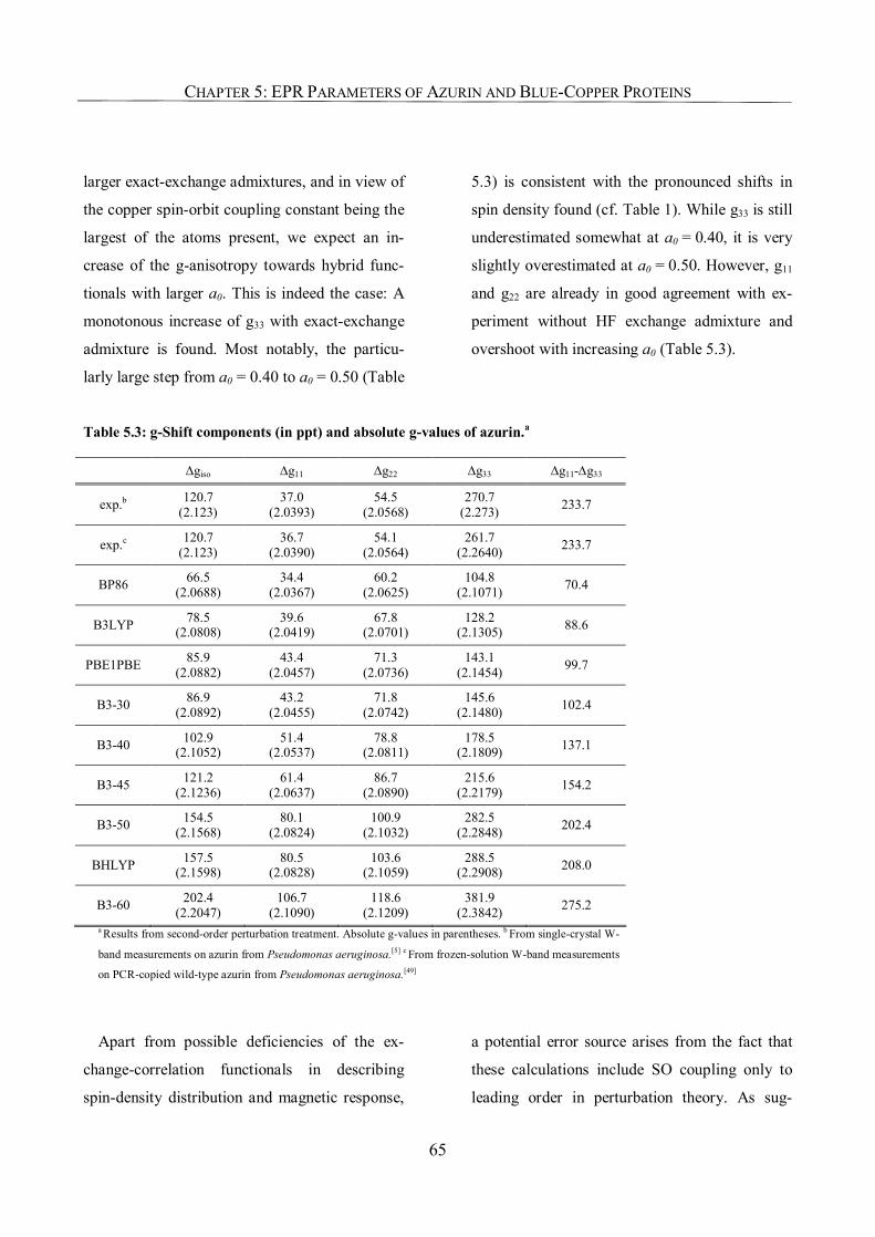
CHAPTER 5: EPR PARAMETERS OF AZURIN AND BLUE-COPPER PROTEINS
65
larger exact-exchange admixtures, and in view of
the copper spin-orbit coupling constant being the
largest of the atoms present, we expect an in-
crease of the g-anisotropy towards hybrid func-
tionals with larger a0. This is indeed the case: A
monotonous increase of g33 with exact-exchange
admixture is found. Most notably, the particu-
larly large step from a0 = 0.40 to a0 = 0.50 (Table
5.3) is consistent with the pronounced shifts in
spin density found (cf. Table 1). While g33 is still
underestimated somewhat at a0 = 0.40, it is very
slightly overestimated at a0 = 0.50. However, g11
and g22 are already in good agreement with ex-
periment without HF exchange admixture and
overshoot with increasing a0 (Table 5.3).
Table 5.3: g-Shift components (in ppt) and absolute g-values of azurin.a
∆giso ∆g11 ∆g22 ∆g33 ∆g11-∆g33
exp.b 120.7 (2.123)
37.0 (2.0393)
54.5 (2.0568)
270.7 (2.273) 233.7
exp.c 120.7 (2.123)
36.7 (2.0390)
54.1 (2.0564)
261.7 (2.2640) 233.7
BP86 66.5 (2.0688)
34.4 (2.0367)
60.2 (2.0625)
104.8 (2.1071) 70.4
B3LYP 78.5 (2.0808)
39.6 (2.0419)
67.8 (2.0701)
128.2 (2.1305) 88.6
PBE1PBE 85.9 (2.0882)
43.4 (2.0457)
71.3 (2.0736)
143.1 (2.1454) 99.7
B3-30 86.9 (2.0892)
43.2 (2.0455)
71.8 (2.0742)
145.6 (2.1480) 102.4
B3-40 102.9 (2.1052)
51.4 (2.0537)
78.8 (2.0811)
178.5 (2.1809) 137.1
B3-45 121.2 (2.1236)
61.4 (2.0637)
86.7 (2.0890)
215.6 (2.2179) 154.2
B3-50 154.5 (2.1568)
80.1 (2.0824)
100.9 (2.1032)
282.5 (2.2848) 202.4
BHLYP 157.5 (2.1598)
80.5 (2.0828)
103.6 (2.1059)
288.5 (2.2908) 208.0
B3-60 202.4 (2.2047)
106.7 (2.1090)
118.6 (2.1209)
381.9 (2.3842) 275.2
a Results from second-order perturbation treatment. Absolute g-values in parentheses. b From single-crystal W-
band measurements on azurin from Pseudomonas aeruginosa.[5] c From frozen-solution W-band measurements
on PCR-copied wild-type azurin from Pseudomonas aeruginosa.[49]
Apart from possible deficiencies of the ex-
change-correlation functionals in describing
spin-density distribution and magnetic response,
a potential error source arises from the fact that
these calculations include SO coupling only to
leading order in perturbation theory. As sug-
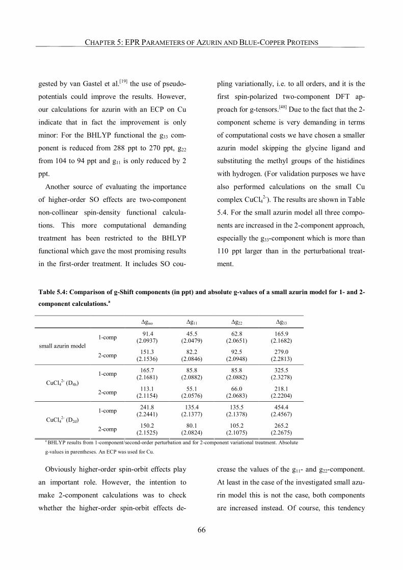
CHAPTER 5: EPR PARAMETERS OF AZURIN AND BLUE-COPPER PROTEINS
66
gested by van Gastel et al.[19] the use of pseudo-
potentials could improve the results. However,
our calculations for azurin with an ECP on Cu
indicate that in fact the improvement is only
minor: For the BHLYP functional the g33 com-
ponent is reduced from 288 ppt to 270 ppt, g22
from 104 to 94 ppt and g11 is only reduced by 2
ppt.
Another source of evaluating the importance
of higher-order SO effects are two-component
non-collinear spin-density functional calcula-
tions. This more computational demanding
treatment has been restricted to the BHLYP
functional which gave the most promising results
in the first-order treatment. It includes SO cou-
pling variationally, i.e. to all orders, and it is the
first spin-polarized two-component DFT ap-
proach for g-tensors.[48] Due to the fact that the 2-
component scheme is very demanding in terms
of computational costs we have chosen a smaller
azurin model skipping the glycine ligand and
substituting the methyl groups of the histidines
with hydrogen. (For validation purposes we have
also performed calculations on the small Cu
complex CuCl42-). The results are shown in Table
5.4. For the small azurin model all three compo-
nents are increased in the 2-component approach,
especially the g33-component which is more than
110 ppt larger than in the perturbational treat-
ment.
Table 5.4: Comparison of g-Shift components (in ppt) and absolute g-values of a small azurin model for 1- and 2-
component calculations.a
∆giso ∆g11 ∆g22 ∆g33
1-comp 91.4 (2.0937)
45.5 (2.0479)
62.8 (2.0651)
165.9 (2.1682)
small azurin model 2-comp 151.3
(2.1536) 82.2
(2.0846) 92.5
(2.0948) 279.0
(2.2813)
1-comp 165.7 (2.1681)
85.8 (2.0882)
85.8 (2.0882)
325.5 (2.3278)
CuCl42- (D4h)
2-comp 113.1 (2.1154)
55.1 (2.0576)
66.0 (2.0683)
218.1 (2.2204)
1-comp 241.8 (2.2441)
135.4 (2.1377)
135.5 (2.1378)
454.4 (2.4567)
CuCl42- (D2d)
2-comp 150.2 (2.1525)
80.1 (2.0824)
105.2 (2.1075)
265.2 (2.2675)
a BHLYP results from 1-component/second-order perturbation and for 2-component variational treatment. Absolute
g-values in parentheses. An ECP was used for Cu.
Obviously higher-order spin-orbit effects play
an important role. However, the intention to
make 2-component calculations was to check
whether the higher-order spin-orbit effects de-
crease the values of the g11- and g22-component.
At least in the case of the investigated small azu-
rin model this is not the case, both components
are increased instead. Of course, this tendency
CHAPTER 5: EPR PARAMETERS OF AZURIN AND BLUE-COPPER PROTEINS
67
needs not to be same for the full azurin model as
we see in the small CuCl42- complexes. Here all
three components are decreased but again the
large effect of higher order spin-orbit effects is
noticeable. The D2d-distorted CuCl42- shows a
significantly larger shifting of the g-tensor than
the D4h-structure and therefore we may conclude
that the change from square-planar to distorted
structures, as present in azurin and other blue-
copper proteins, is responsible for such large SO
effects. Actually this is also seen in the second-
order SO contributions to HFCs as we will dis-
cuss in the next sections.
5.3.4. 65Cu Hyperfine Coupling Constants
The second EPR probe of spin-density distri-
bution we evaluate is the copper hyperfine cou-
pling tensors. Together with the blue color, the
unusually small A|| component (and a resulting
small isotropic coupling Aiso) is the most striking
spectroscopic characteristic of blue copper pro-
teins compared to “normal” CuII complexes. A
series of experimental and computational studies
by Solomon and coworkers[15, 42] (see introduc-
tory section) suggested that the small A|| value
reflects mainly the unusually large Cu-S(Cys)
covalency. Our computational results for azurin,
plastocyanin and stellacyanin in Table 5.5 indi-
cate, however, that rationalization by a particu-
larly small metal spin density is an unacceptable
oversimplification.
Let us start with azurin, for which the most ex-
tensive comparison of functionals has been car-
ried out (Table 5.5). First of all, the overall iso-
tropic hyperfine coupling starts out appreciably
negative for the BP86 GGA functional and
grows to less negative values with larger Har-
tree-Fock exchange admixtures a0. How can this
be reconciled with increasing metal spin density
along the same series of functionals (cf. Table
5.1)? Closer examination of the first- and sec-
ond-order contributions indicates that the first-
order Fermi-contact term AFC is substantially
negative already with BP86 and turns even more
negative with increasing a0. This is the expected
trend, as the negative spin density at the copper
nucleus arises from spin polarization of the 2s
(large negative contribution) and 3s (smaller
positive contribution) core shells by the unpaired
spin density in the copper 3d orbitals.[28, 29] Thus,
the increased spin density on copper with in-
creasing a0 causes a more negative AFC value. At
the same time, however, the pseudocontact term,
APC (i.e. the second-order SO correction to Aiso)
is significant and positive already at BP86 level
and increases even more dramatically in absolute
value with increasing a0. As a result, Aiso turns
less negative and arrives at a very small absolute
value at BHLYP level (still about 27 MHz too
large compared to experiment). We want to note
in passing, that spin-orbit effects to the Cu HFCs
are crucial to take into account and that calcula-
tions which neglect these effects will lead to
inaccurate results (see refs. [50] and [51]).
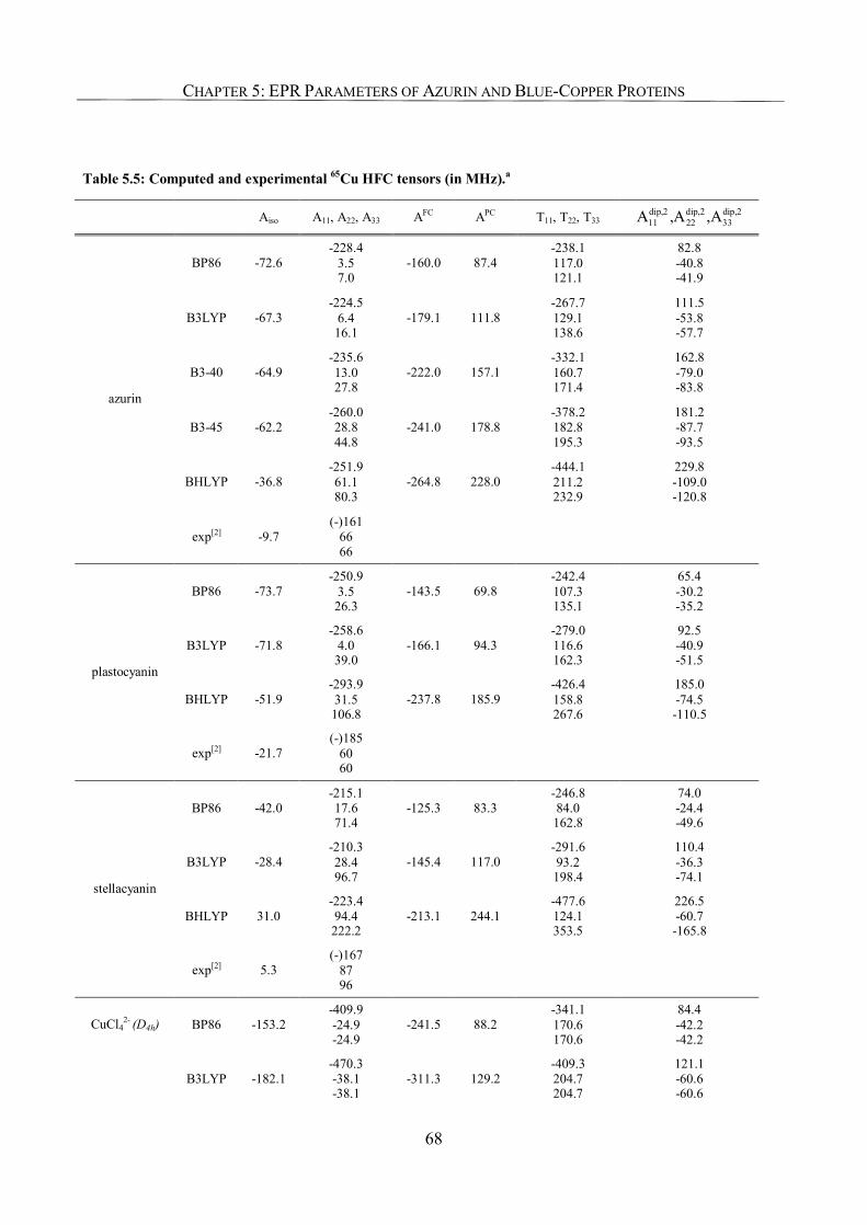
CHAPTER 5: EPR PARAMETERS OF AZURIN AND BLUE-COPPER PROTEINS
68
Table 5.5: Computed and experimental 65Cu HFC tensors (in MHz).a
Aiso A11, A22, A33 AFC APC T11, T22, T33 dip,2 dip,2 dip,211 22 33A ,A ,A
BP86 -72.6 -228.4
3.5 7.0
-160.0 87.4 -238.1 117.0 121.1
82.8 -40.8 -41.9
B3LYP -67.3 -224.5
6.4 16.1
-179.1 111.8 -267.7 129.1 138.6
111.5 -53.8 -57.7
B3-40 -64.9 -235.6 13.0 27.8
-222.0 157.1 -332.1 160.7 171.4
162.8 -79.0 -83.8
B3-45 -62.2 -260.0 28.8 44.8
-241.0 178.8 -378.2 182.8 195.3
181.2 -87.7 -93.5
BHLYP -36.8 -251.9 61.1 80.3
-264.8 228.0 -444.1 211.2 232.9
229.8 -109.0 -120.8
azurin
exp[2] -9.7 (-)161
66 66
BP86 -73.7 -250.9
3.5 26.3
-143.5 69.8 -242.4 107.3 135.1
65.4 -30.2 -35.2
B3LYP -71.8 -258.6
4.0 39.0
-166.1 94.3 -279.0 116.6 162.3
92.5 -40.9 -51.5
BHLYP -51.9 -293.9 31.5 106.8
-237.8 185.9 -426.4 158.8 267.6
185.0 -74.5 -110.5
plastocyanin
exp[2] -21.7 (-)185
60 60
BP86 -42.0 -215.1 17.6 71.4
-125.3 83.3 -246.8 84.0 162.8
74.0 -24.4 -49.6
B3LYP -28.4 -210.3 28.4 96.7
-145.4 117.0 -291.6 93.2 198.4
110.4 -36.3 -74.1
BHLYP 31.0 -223.4 94.4 222.2
-213.1 244.1 -477.6 124.1 353.5
226.5 -60.7 -165.8
stellacyanin
exp[2] 5.3 (-)167
87 96
BP86 -153.2 -409.9 -24.9 -24.9
-241.5 88.2 -341.1 170.6 170.6
84.4 -42.2 -42.2
CuCl42- (D4h)
B3LYP -182.1 -470.3 -38.1 -38.1
-311.3 129.2 -409.3 204.7 204.7
121.1 -60.6 -60.6
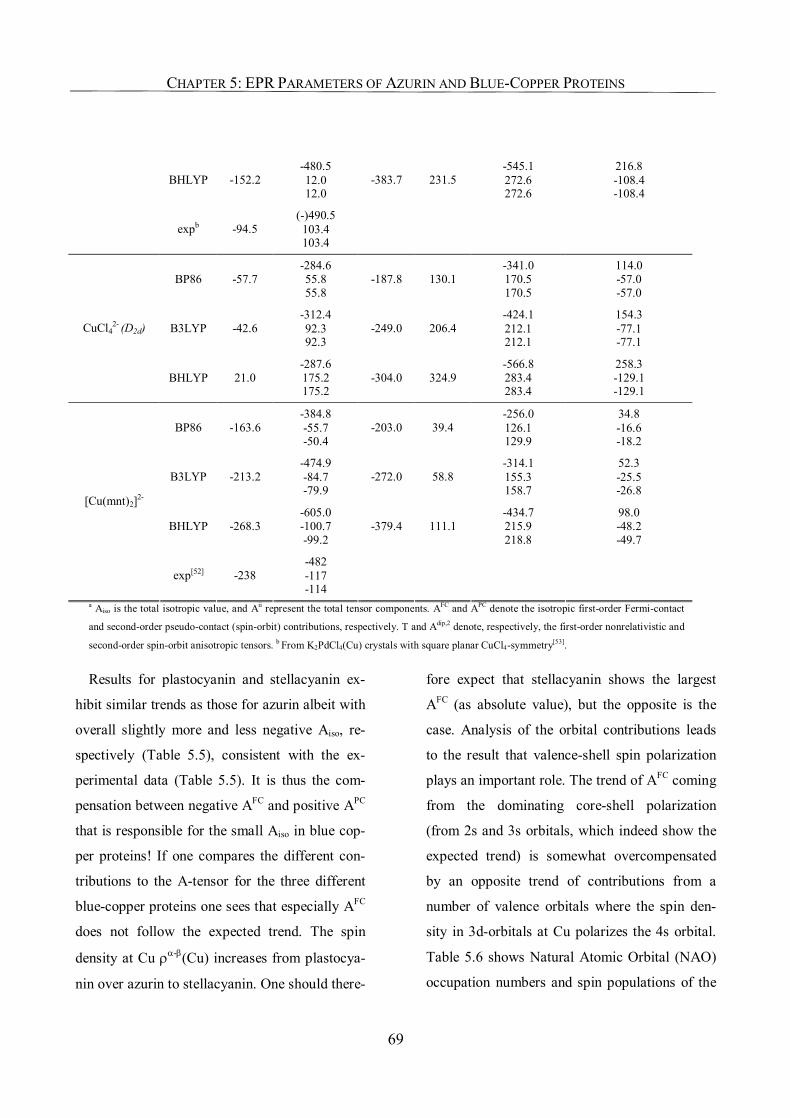
CHAPTER 5: EPR PARAMETERS OF AZURIN AND BLUE-COPPER PROTEINS
69
BHLYP -152.2 -480.5 12.0 12.0
-383.7 231.5 -545.1 272.6 272.6
216.8 -108.4 -108.4
expb -94.5 (-)490.5 103.4 103.4
BP86 -57.7 -284.6 55.8 55.8
-187.8 130.1 -341.0 170.5 170.5
114.0 -57.0 -57.0
B3LYP -42.6 -312.4 92.3 92.3
-249.0 206.4 -424.1 212.1 212.1
154.3 -77.1 -77.1
CuCl42- (D2d)
BHLYP 21.0 -287.6 175.2 175.2
-304.0 324.9 -566.8 283.4 283.4
258.3 -129.1 -129.1
BP86 -163.6 -384.8 -55.7 -50.4
-203.0 39.4 -256.0 126.1 129.9
34.8 -16.6 -18.2
B3LYP -213.2 -474.9 -84.7 -79.9
-272.0 58.8 -314.1 155.3 158.7
52.3 -25.5 -26.8
BHLYP -268.3 -605.0 -100.7 -99.2
-379.4 111.1 -434.7 215.9 218.8
98.0 -48.2 -49.7
[Cu(mnt)2]2-
exp[52] -238 -482 -117 -114
a Aiso is the total isotropic value, and Aii represent the total tensor components. AFC and APC denote the isotropic first-order Fermi-contact
and second-order pseudo-contact (spin-orbit) contributions, respectively. T and Adip,2 denote, respectively, the first-order nonrelativistic and
second-order spin-orbit anisotropic tensors. b From K2PdCl4(Cu) crystals with square planar CuCl4-symmetry[53].
Results for plastocyanin and stellacyanin ex-
hibit similar trends as those for azurin albeit with
overall slightly more and less negative Aiso, re-
spectively (Table 5.5), consistent with the ex-
perimental data (Table 5.5). It is thus the com-
pensation between negative AFC and positive APC
that is responsible for the small Aiso in blue cop-
per proteins! If one compares the different con-
tributions to the A-tensor for the three different
blue-copper proteins one sees that especially AFC
does not follow the expected trend. The spin
density at Cu ρα-β(Cu) increases from plastocya-
nin over azurin to stellacyanin. One should there-
fore expect that stellacyanin shows the largest
AFC (as absolute value), but the opposite is the
case. Analysis of the orbital contributions leads
to the result that valence-shell spin polarization
plays an important role. The trend of AFC coming
from the dominating core-shell polarization
(from 2s and 3s orbitals, which indeed show the
expected trend) is somewhat overcompensated
by an opposite trend of contributions from a
number of valence orbitals where the spin den-
sity in 3d-orbitals at Cu polarizes the 4s orbital.
Table 5.6 shows Natural Atomic Orbital (NAO)
occupation numbers and spin populations of the
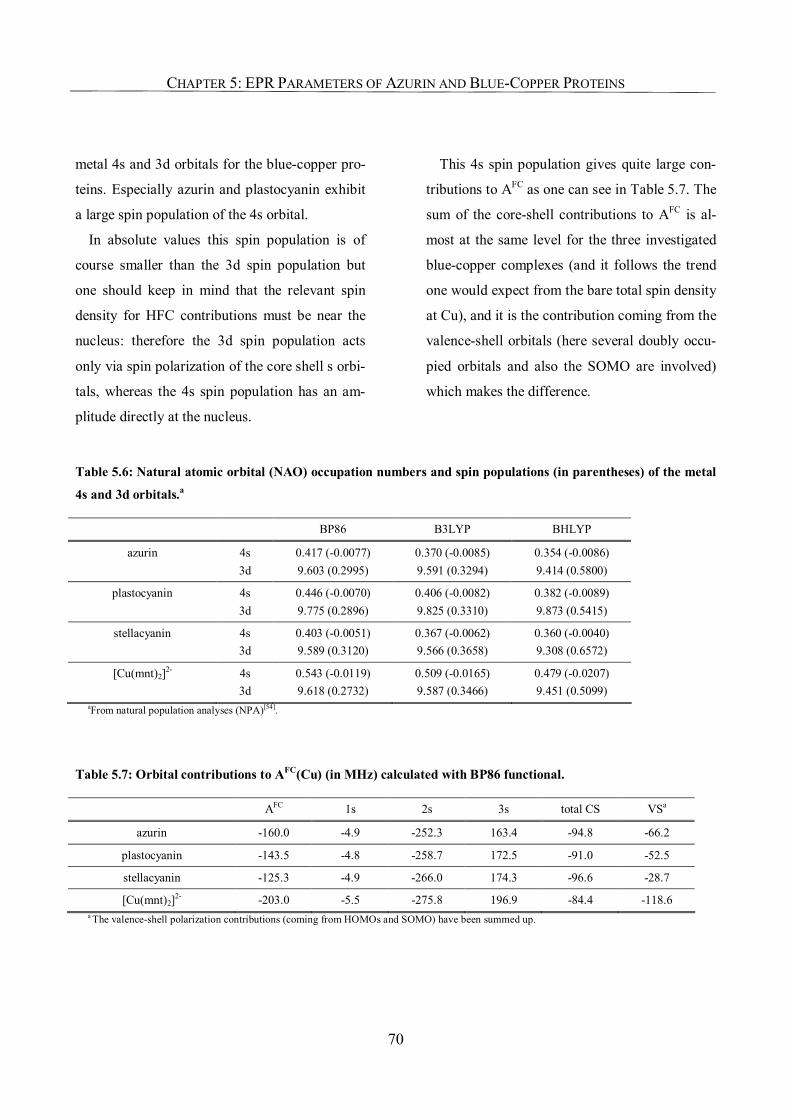
CHAPTER 5: EPR PARAMETERS OF AZURIN AND BLUE-COPPER PROTEINS
70
metal 4s and 3d orbitals for the blue-copper pro-
teins. Especially azurin and plastocyanin exhibit
a large spin population of the 4s orbital.
In absolute values this spin population is of
course smaller than the 3d spin population but
one should keep in mind that the relevant spin
density for HFC contributions must be near the
nucleus: therefore the 3d spin population acts
only via spin polarization of the core shell s orbi-
tals, whereas the 4s spin population has an am-
plitude directly at the nucleus.
This 4s spin population gives quite large con-
tributions to AFC as one can see in Table 5.7. The
sum of the core-shell contributions to AFC is al-
most at the same level for the three investigated
blue-copper complexes (and it follows the trend
one would expect from the bare total spin density
at Cu), and it is the contribution coming from the
valence-shell orbitals (here several doubly occu-
pied orbitals and also the SOMO are involved)
which makes the difference.
Table 5.6: Natural atomic orbital (NAO) occupation numbers and spin populations (in parentheses) of the metal
4s and 3d orbitals.a
BP86 B3LYP BHLYP
azurin 4s 3d
0.417 (-0.0077) 9.603 (0.2995)
0.370 (-0.0085) 9.591 (0.3294)
0.354 (-0.0086) 9.414 (0.5800)
plastocyanin 4s 3d
0.446 (-0.0070) 9.775 (0.2896)
0.406 (-0.0082) 9.825 (0.3310)
0.382 (-0.0089) 9.873 (0.5415)
stellacyanin 4s 3d
0.403 (-0.0051) 9.589 (0.3120)
0.367 (-0.0062) 9.566 (0.3658)
0.360 (-0.0040) 9.308 (0.6572)
[Cu(mnt)2]2- 4s 3d
0.543 (-0.0119) 9.618 (0.2732)
0.509 (-0.0165) 9.587 (0.3466)
0.479 (-0.0207) 9.451 (0.5099)
aFrom natural population analyses (NPA)[54].
Table 5.7: Orbital contributions to AFC(Cu) (in MHz) calculated with BP86 functional.
AFC 1s 2s 3s total CS VSa
azurin -160.0 -4.9 -252.3 163.4 -94.8 -66.2
plastocyanin -143.5 -4.8 -258.7 172.5 -91.0 -52.5
stellacyanin -125.3 -4.9 -266.0 174.3 -96.6 -28.7
[Cu(mnt)2]2- -203.0 -5.5 -275.8 196.9 -84.4 -118.6 a The valence-shell polarization contributions (coming from HOMOs and SOMO) have been summed up.
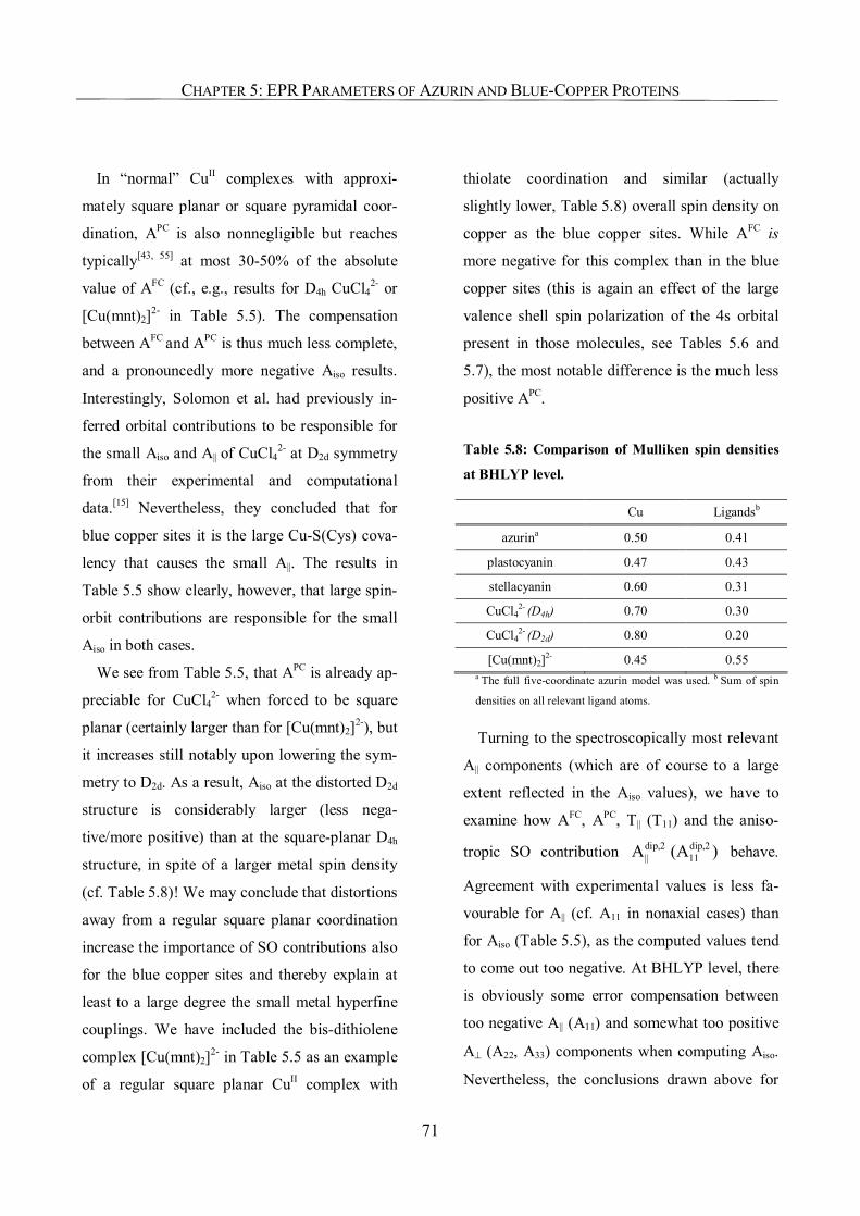
CHAPTER 5: EPR PARAMETERS OF AZURIN AND BLUE-COPPER PROTEINS
71
In “normal” CuII complexes with approxi-
mately square planar or square pyramidal coor-
dination, APC is also nonnegligible but reaches
typically[43, 55] at most 30-50% of the absolute
value of AFC (cf., e.g., results for D4h CuCl42- or
[Cu(mnt)2]2- in Table 5.5). The compensation
between AFC and APC is thus much less complete,
and a pronouncedly more negative Aiso results.
Interestingly, Solomon et al. had previously in-
ferred orbital contributions to be responsible for
the small Aiso and A|| of CuCl4
2- at D2d symmetry
from their experimental and computational
data.[15] Nevertheless, they concluded that for
blue copper sites it is the large Cu-S(Cys) cova-
lency that causes the small A||. The results in
Table 5.5 show clearly, however, that large spin-
orbit contributions are responsible for the small
Aiso in both cases.
We see from Table 5.5, that APC is already ap-
preciable for CuCl42- when forced to be square
planar (certainly larger than for [Cu(mnt)2]2-), but
it increases still notably upon lowering the sym-
metry to D2d. As a result, Aiso at the distorted D2d
structure is considerably larger (less nega-
tive/more positive) than at the square-planar D4h
structure, in spite of a larger metal spin density
(cf. Table 5.8)! We may conclude that distortions
away from a regular square planar coordination
increase the importance of SO contributions also
for the blue copper sites and thereby explain at
least to a large degree the small metal hyperfine
couplings. We have included the bis-dithiolene
complex [Cu(mnt)2]2- in Table 5.5 as an example
of a regular square planar CuII complex with
thiolate coordination and similar (actually
slightly lower, Table 5.8) overall spin density on
copper as the blue copper sites. While AFC is
more negative for this complex than in the blue
copper sites (this is again an effect of the large
valence shell spin polarization of the 4s orbital
present in those molecules, see Tables 5.6 and
5.7), the most notable difference is the much less
positive APC.
Table 5.8: Comparison of Mulliken spin densities
at BHLYP level.
Cu Ligandsb
azurina 0.50 0.41
plastocyanin 0.47 0.43
stellacyanin 0.60 0.31
CuCl42- (D4h) 0.70 0.30
CuCl42- (D2d) 0.80 0.20
[Cu(mnt)2]2- 0.45 0.55 a The full five-coordinate azurin model was used. b Sum of spin
densities on all relevant ligand atoms.
Turning to the spectroscopically most relevant
A|| components (which are of course to a large
extent reflected in the Aiso values), we have to
examine how AFC, APC, T|| (T11) and the aniso-
tropic SO contribution dip,2 dip,2|| 11A (A ) behave.
Agreement with experimental values is less fa-
vourable for A|| (cf. A11 in nonaxial cases) than
for Aiso (Table 5.5), as the computed values tend
to come out too negative. At BHLYP level, there
is obviously some error compensation between
too negative A|| (A11) and somewhat too positive
A⊥ (A22, A33) components when computing Aiso.
Nevertheless, the conclusions drawn above for
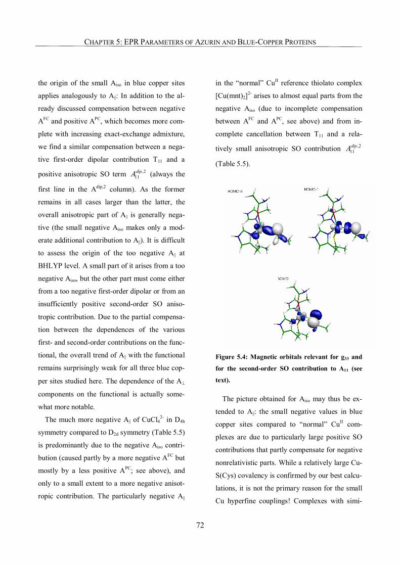
CHAPTER 5: EPR PARAMETERS OF AZURIN AND BLUE-COPPER PROTEINS
72
the origin of the small Aiso in blue copper sites
applies analogously to A||: In addition to the al-
ready discussed compensation between negative
AFC and positive APC, which becomes more com-
plete with increasing exact-exchange admixture,
we find a similar compensation between a nega-
tive first-order dipolar contribution T11 and a
positive anisotropic SO term ,211dipA (always the
first line in the Adip,2 column). As the former
remains in all cases larger than the latter, the
overall anisotropic part of A|| is generally nega-
tive (the small negative Aiso makes only a mod-
erate additional contribution to A||). It is difficult
to assess the origin of the too negative A|| at
BHLYP level. A small part of it arises from a too
negative Aiso, but the other part must come either
from a too negative first-order dipolar or from an
insufficiently positive second-order SO aniso-
tropic contribution. Due to the partial compensa-
tion between the dependences of the various
first- and second-order contributions on the func-
tional, the overall trend of A|| with the functional
remains surprisingly weak for all three blue cop-
per sites studied here. The dependence of the A⊥
components on the functional is actually some-
what more notable.
The much more negative A|| of CuCl42- in D4h
symmetry compared to D2d symmetry (Table 5.5)
is predominantly due to the negative Aiso contri-
bution (caused partly by a more negative AFC but
mostly by a less positive APC; see above), and
only to a small extent to a more negative anisot-
ropic contribution. The particularly negative A||
in the “normal” CuII reference thiolato complex
[Cu(mnt)2]2- arises to almost equal parts from the
negative Aiso (due to incomplete compensation
between AFC and APC, see above) and from in-
complete cancellation between T11 and a rela-
tively small anisotropic SO contribution ,211dipA
(Table 5.5).
Figure 5.4: Magnetic orbitals relevant for g33 and
for the second-order SO contribution to A11 (see
text).
The picture obtained for Aiso may thus be ex-
tended to A||: the small negative values in blue
copper sites compared to “normal” CuII com-
plexes are due to particularly large positive SO
contributions that partly compensate for negative
nonrelativistic parts. While a relatively large Cu-
S(Cys) covalency is confirmed by our best calcu-
lations, it is not the primary reason for the small
Cu hyperfine couplings! Complexes with simi-
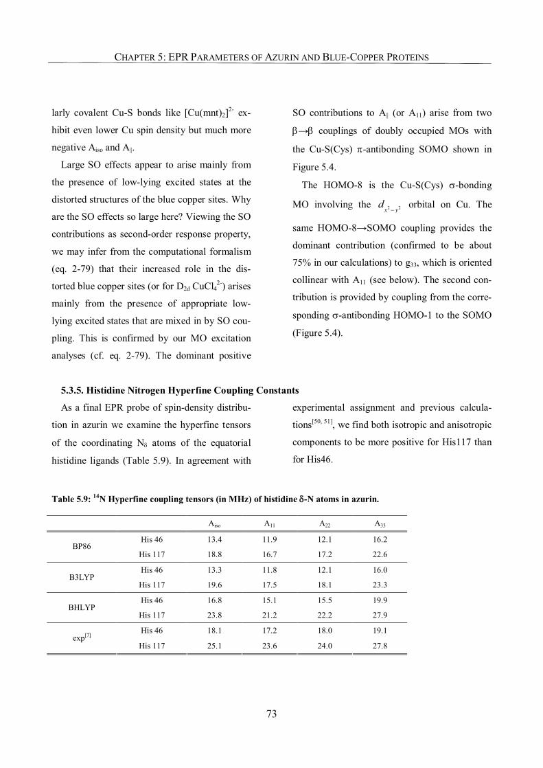
CHAPTER 5: EPR PARAMETERS OF AZURIN AND BLUE-COPPER PROTEINS
73
larly covalent Cu-S bonds like [Cu(mnt)2]2- ex-
hibit even lower Cu spin density but much more
negative Aiso and A||.
Large SO effects appear to arise mainly from
the presence of low-lying excited states at the
distorted structures of the blue copper sites. Why
are the SO effects so large here? Viewing the SO
contributions as second-order response property,
we may infer from the computational formalism
(eq. 2-79) that their increased role in the dis-
torted blue copper sites (or for D2d CuCl42-) arises
mainly from the presence of appropriate low-
lying excited states that are mixed in by SO cou-
pling. This is confirmed by our MO excitation
analyses (cf. eq. 2-79). The dominant positive
SO contributions to A|| (or A11) arise from two
β→β couplings of doubly occupied MOs with
the Cu-S(Cys) π-antibonding SOMO shown in
Figure 5.4.
The HOMO-8 is the Cu-S(Cys) σ-bonding
MO involving the 2 2x yd
− orbital on Cu. The
same HOMO-8→SOMO coupling provides the
dominant contribution (confirmed to be about
75% in our calculations) to g33, which is oriented
collinear with A11 (see below). The second con-
tribution is provided by coupling from the corre-
sponding σ-antibonding HOMO-1 to the SOMO
(Figure 5.4).
5.3.5. Histidine Nitrogen Hyperfine Coupling Constants
As a final EPR probe of spin-density distribu-
tion in azurin we examine the hyperfine tensors
of the coordinating Nδ atoms of the equatorial
histidine ligands (Table 5.9). In agreement with
experimental assignment and previous calcula-
tions[50, 51], we find both isotropic and anisotropic
components to be more positive for His117 than
for His46.
Table 5.9: 14N Hyperfine coupling tensors (in MHz) of histidine δ-N atoms in azurin.
Aiso A11 A22 A33
His 46 13.4 11.9 12.1 16.2 BP86
His 117 18.8 16.7 17.2 22.6
His 46 13.3 11.8 12.1 16.0 B3LYP
His 117 19.6 17.5 18.1 23.3
His 46 16.8 15.1 15.5 19.9 BHLYP
His 117 23.8 21.2 22.2 27.9
His 46 18.1 17.2 18.0 19.1 exp[7]
His 117 25.1 23.6 24.0 27.8
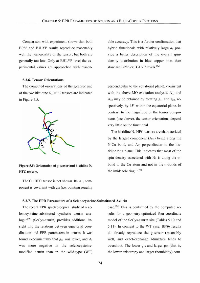
CHAPTER 5: EPR PARAMETERS OF AZURIN AND BLUE-COPPER PROTEINS
74
Comparison with experiment shows that both
BP86 and B3LYP results reproduce reasonably
well the near-axiality of the tensor, but both are
generally too low. Only at BHLYP level the ex-
perimental values are approached with reason-
able accuracy. This is a further confirmation that
hybrid functionals with relatively large a0 pro-
vide a better description of the overall spin-
density distribution in blue copper sites than
standard BP86 or B3LYP levels.[42]
5.3.6. Tensor Orientations
The computed orientations of the g-tensor and
of the two histidine Nδ HFC tensors are indicated
in Figure 5.5.
Figure 5.5: Orientation of g-tensor and histidine Nδ
HFC tensors.
The Cu HFC tensor is not shown. Its A11 com-
ponent is covariant with g33 (i.e. pointing roughly
perpendicular to the equatorial plane), consistent
with the above MO excitation analysis. A22 and
A33 may be obtained by rotating g11 and g22, re-
spectively, by 45° within the equatorial plane. In
contrast to the magnitude of the tensor compo-
nents (see above), the tensor orientations depend
very little on the functional.
The histidine Nδ HFC tensors are characterized
by the largest component (A33) being along the
N-Cu bond, and A22 perpendicular to the his-
tidine ring plane. This indicates that most of the
spin density associated with Nδ is along the σ-
bond to the Cu atom and not in the π-bonds of
the imidazole ring.[7, 56]
5.3.7. The EPR Parameters of a Selenocysteine-Substituted Azurin
The recent EPR spectroscopical study of a se-
lenocysteine-substituted synthetic azurin ana-
logue[49] (SeCys-azurin) provides additional in-
sight into the relations between equatorial coor-
dination and EPR parameters in azurin. It was
found experimentally that g33 was lower, and A||
was more negative in the selenocysteine-
modified azurin than in the wild-type (WT)
case.[49] This is confirmed by the computed re-
sults for a geometry-optimized four-coordinate
model of the SeCys-azurin site (Tables 5.10 and
5.11). In contrast to the WT case, BP86 results
do already reproduce the g-tensor reasonably
well, and exact-exchange admixture tends to
overshoot. The lower g33 and larger g22 (that is,
the lower anisotropy and larger rhombicity) com-
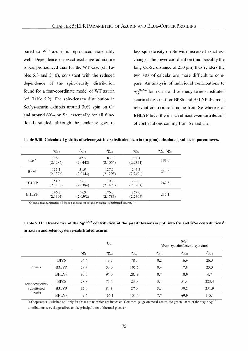
CHAPTER 5: EPR PARAMETERS OF AZURIN AND BLUE-COPPER PROTEINS
75
pared to WT azurin is reproduced reasonably
well. Dependence on exact-exchange admixture
is less pronounced than for the WT case (cf. Ta-
bles 5.3 and 5.10), consistent with the reduced
dependence of the spin-density distribution
found for a four-coordinate model of WT azurin
(cf. Table 5.2). The spin-density distribution in
SeCys-azurin exhibits around 30% spin on Cu
and around 60% on Se, essentially for all func-
tionals studied, although the tendency goes to
less spin density on Se with increased exact ex-
change. The lower coordination (and possibly the
long Cu-Se distance of 230 pm) thus renders the
two sets of calculations more difficult to com-
pare. An analysis of individual contributions to
∆gSO/OZ for azurin and selenocysteine-substituted
azurin shows that for BP86 and B3LYP the most
relevant contributions come from Se whereas at
BHLYP level there is an almost even distribution
of contributions coming from Se and Cu.
Table 5.10: Calculated g-shifts of selenocysteine-substituted azurin (in ppm), absolute g-values in parentheses.
∆giso ∆g11 ∆g22 ∆g33 ∆g33-∆g11
exp.a 126.3 (2.1286)
42.5 (2.0448)
103.3 (2.1056)
233.1 (2.2354) 188.6
BP86 135.1 (2.1376)
31.9 (2.0344)
127.0 (2.1293)
246.5 (2.2491) 214.6
B3LYP 151.5 (2.1538)
36.1 (2.0384)
140.0 (2.1423)
278.6 (2.2809) 242.5
BHLYP 166.7 (2.1691)
56.9 (2.0592)
176.3 (2.1786)
267.0 (2.2693) 210.1
a Q-band measurements of frozen glasses of selenocysteine-substituted azurin. [49]
Table 5.11: Breakdown of the ∆gSO/OZ contribution of the g-shift tensor (in ppt) into Cu and S/Se contributionsa
in azurin and selenocysteine-substituted azurin.
Cu S/Se (from cysteine/seleno-cysteine)
∆g11 ∆g22 ∆g33 ∆g11 ∆g22 ∆g33
BP86 34.4 43.7 78.3 0.2 16.6 26.3
B3LYP 39.4 50.0 102.5 0.4 17.8 25.5 azurin
BHLYP 80.0 94.0 283.9 0.7 10.0 4.7
BP86 28.8 75.4 23.0 3.1 51.4 223.4
B3LYP 32.9 89.3 27.0 3.5 50.2 251.9 selenocysteine-
substituted azurin
BHLYP 49.6 106.1 151.4 7.7 69.0 115.1 a SO operators “switched on” only for those atoms which are indicated. Common gauge on metal center, the general axes of the single ∆gSO/OZ
contributions were diagonalized on the principal axes of the total g tensor.
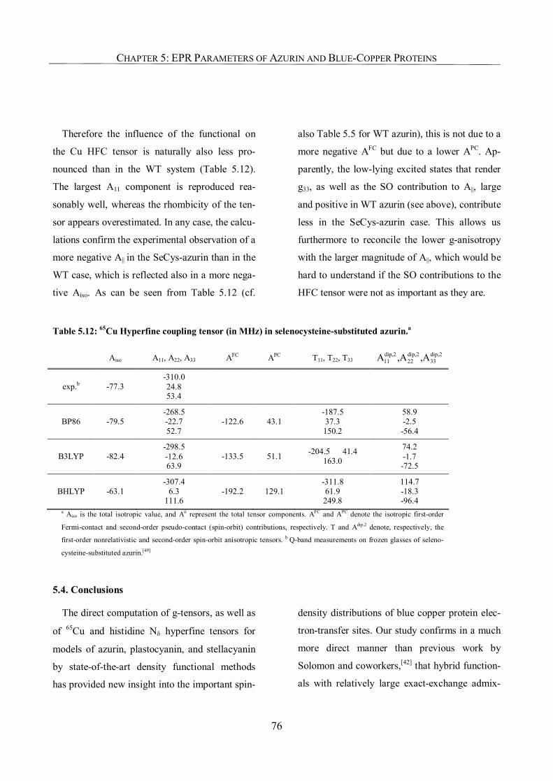
CHAPTER 5: EPR PARAMETERS OF AZURIN AND BLUE-COPPER PROTEINS
76
Therefore the influence of the functional on
the Cu HFC tensor is naturally also less pro-
nounced than in the WT system (Table 5.12).
The largest A11 component is reproduced rea-
sonably well, whereas the rhombicity of the ten-
sor appears overestimated. In any case, the calcu-
lations confirm the experimental observation of a
more negative A|| in the SeCys-azurin than in the
WT case, which is reflected also in a more nega-
tive Aiso. As can be seen from Table 5.12 (cf.
also Table 5.5 for WT azurin), this is not due to a
more negative AFC but due to a lower APC. Ap-
parently, the low-lying excited states that render
g33, as well as the SO contribution to A||, large
and positive in WT azurin (see above), contribute
less in the SeCys-azurin case. This allows us
furthermore to reconcile the lower g-anisotropy
with the larger magnitude of A||, which would be
hard to understand if the SO contributions to the
HFC tensor were not as important as they are.
Table 5.12: 65Cu Hyperfine coupling tensor (in MHz) in selenocysteine-substituted azurin.a
Aiso A11, A22, A33 AFC APC T11, T22, T33 dip,2 dip,2 dip,211 22 33A ,A ,A
exp.b -77.3 -310.0 24.8 53.4
BP86 -79.5 -268.5 -22.7 52.7
-122.6 43.1 -187.5 37.3 150.2
58.9 -2.5 -56.4
B3LYP -82.4 -298.5 -12.6 63.9
-133.5 51.1 -204.5 41.4 163.0
74.2 -1.7 -72.5
BHLYP -63.1 -307.4
6.3 111.6
-192.2 129.1 -311.8 61.9 249.8
114.7 -18.3 -96.4
a Aiso is the total isotropic value, and Aii represent the total tensor components. AFC and APC denote the isotropic first-order
Fermi-contact and second-order pseudo-contact (spin-orbit) contributions, respectively. T and Adip,2 denote, respectively, the
first-order nonrelativistic and second-order spin-orbit anisotropic tensors. b Q-band measurements on frozen glasses of seleno-
cysteine-substituted azurin.[49]
5.4. Conclusions
The direct computation of g-tensors, as well as
of 65Cu and histidine Nδ hyperfine tensors for
models of azurin, plastocyanin, and stellacyanin
by state-of-the-art density functional methods
has provided new insight into the important spin-
density distributions of blue copper protein elec-
tron-transfer sites. Our study confirms in a much
more direct manner than previous work by
Solomon and coworkers,[42] that hybrid function-
als with relatively large exact-exchange admix-
CHAPTER 5: EPR PARAMETERS OF AZURIN AND BLUE-COPPER PROTEINS
77
tures provide an improved description of the
spin-density distribution in blue copper sites
compared to more standard BP86 or B3LYP
functionals. The spin density is distributed to
approximately equal shares between Cu and the
equatorially coordinating S(Cys) atom. In spite
of the confirmed appreciable covalency in that
bond, our calculations provide a different expla-
nation for the small Cu A|| hyperfine than as-
sumed hitherto: Near-complete cancellation be-
tween negative Fermi-contact and dipolar and
appreciable positive second-order spin-orbit con-
tributions are responsible for the characteristic
small copper hyperfine couplings in blue copper
sites. For example dithiolene complexes with
regular square planar coordination of CuII exhibit
even less Cu spin density but much larger nega-
tive A|| than blue copper sites.
Closer examination indicates that the distorted,
essentially trigonal structure of the blue copper
sites and the equatorially coordinated cysteine
ligand provide access to low-lying excited states
that are coupled strongly to the ground state by
spin-orbit coupling. Both the large g-anisotropy
and the large spin-orbit contributions to the Cu
hyperfine coupling (and thus the small Cu A|| and
Aiso) derive from these strong couplings. A fur-
ther indication for this coupling is the large in-
fluence of higher-order spin-orbit contributions
which is shown by two-component relativistic g-
tensor calculations.
Studies on a selenocystein-substituted azurin
analogue have provided additional insight into
the relations between structure, bonding, and
EPR parameters in blue copper protein sites.
78
79
Chapter 6
Where is the Spin? Understanding Electronic Struc-
ture and g-Tensors for Ruthenium Complexes with
Redox-Active Quinonoid Ligands[1]
6.1. Introduction
Redox-active ligands, sometimes termed “non-
innocent” ligands, may occur in several different
formal oxidation states, e.g. when bound to a
transition metal.[2,3] Complexes with redox-active
ligands are of tremendous importance in many
redox processes, in particular when the transfer
of more than one electron is required, e.g. in
certain metalloenzymes.[4] Prime examples in
nature are tetrapyrrol-based ligands (e.g. por-
phyrins), pterins, flavins, quinones, dithiolenes,
or phenoxyl-based systems. The possible change
of ligand oxidation state makes it difficult to
assign unambiguous “physical”[5] oxidation
numbers to the metal center. In open-shell cases,
EPR spectroscopy has often been used to esti-
mate the spin distribution from experimental
data, and to subsequently assign oxidation num-
bers. Quantum chemical calculations provide
independent access to EPR parameters, and to
density and spin-density distributions. As spin
delocalization and spin polarization mechanisms
tend to be pronounced in transition metal sys-
tems, the use of quantum-chemical methods has
proven to provide particularly valuable insights
into electronic structure,[6-8] and thus indirectly
into physical oxidation states, provided that a
clearcut assignment of charge and/or spin to
metal and ligands is possible.
In this chapter we will evaluate g-tensors and
spin-density distributions of a series of anionic
and cationic ruthenium complexes with o-
quinonoid ligands. DFT is well suited for spin
density analyses of transition metal complexes
even of appreciable size, as has been shown re-
cently, e.g., by comparison to post-Hartree-Fock
spin densities for iron porphyrin complexes.[9]
The particular systems we have chosen here are
based on a recent experimental study by Patra
et.al.[10] Using X-ray and EPR methods, they
investigated complexes [Ru(acac)2L]+1/0/-1, where
L is an o-iminoquinone or o-iminothioquinone
(Figure 6.1 provides examples for the two ex-
perimentally studied cases). o-Quinone-type
ligands have received particular attention from
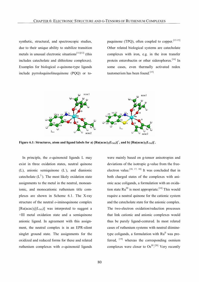
CHAPTER 6: ELECTRONIC STRUCTURE AND G-TENSORS OF RUTHENIUM COMPLEXES
80
synthetic, structural, and spectroscopic studies,
due to their unique ability to stabilize transition
metals in unusual electronic situations[11][12] (this
includes catecholate and dithiolene complexes).
Examples for biological o-quinone-type ligands
include pyrroloquinolinequinone (PQQ) or to-
paquinone (TPQ), often coupled to copper.[13-15]
Other related biological systems are catecholate
complexes with iron, e.g. in the iron transfer
protein enterobactin or other siderophores.[16] In
some cases, even thermally activated redox
tautomerism has been found.[15]
Figure 6.1: Structures, atom and ligand labels for a) [Ru(acac)2(LNO)]+, and b) [Ru(acac)2(LNS)]-.
In principle, the o-quinonoid ligands L may
exist in three oxidation states, neutral quinone
(L), anionic semiquinone (L-), and dianionic
catecholate (L2-). The most likely oxidation state
assignments to the metal in the neutral, monoan-
ionic, and monocationic ruthenium title com-
plexes are shown in Scheme 6.1. The X-ray
structure of the neutral o-iminoquinone complex
[Ru(acac)2[(LNO)] was interpreted to suggest a
+III metal oxidation state and a semiquinone
anionic ligand. In agreement with this assign-
ment, the neutral complex is in an EPR-silent
singlet ground state. The assignments for the
oxidized and reduced forms for these and related
ruthenium complexes with o-quinonoid ligands
were mainly based on g-tensor anisotropies and
deviations of the isotropic g-value from the free-
electron value.[10, 17, 18] It was concluded that in
both charged states of the complexes with ani-
onic acac coligands, a formulation with an oxida-
tion state RuIII is most appropriate.[10] This would
require a neutral quinone for the cationic system
and the catecholate state for the anionic complex.
The two-electron oxidation/reduction processes
that link cationic and anionic complexes would
thus be purely ligand-centered. In most related
cases of ruthenium systems with neutral diimine-
type coligands, a formulation with RuII was pre-
ferred, [19] whereas the corresponding osmium
complexes were closer to OsIII.[20] Very recently
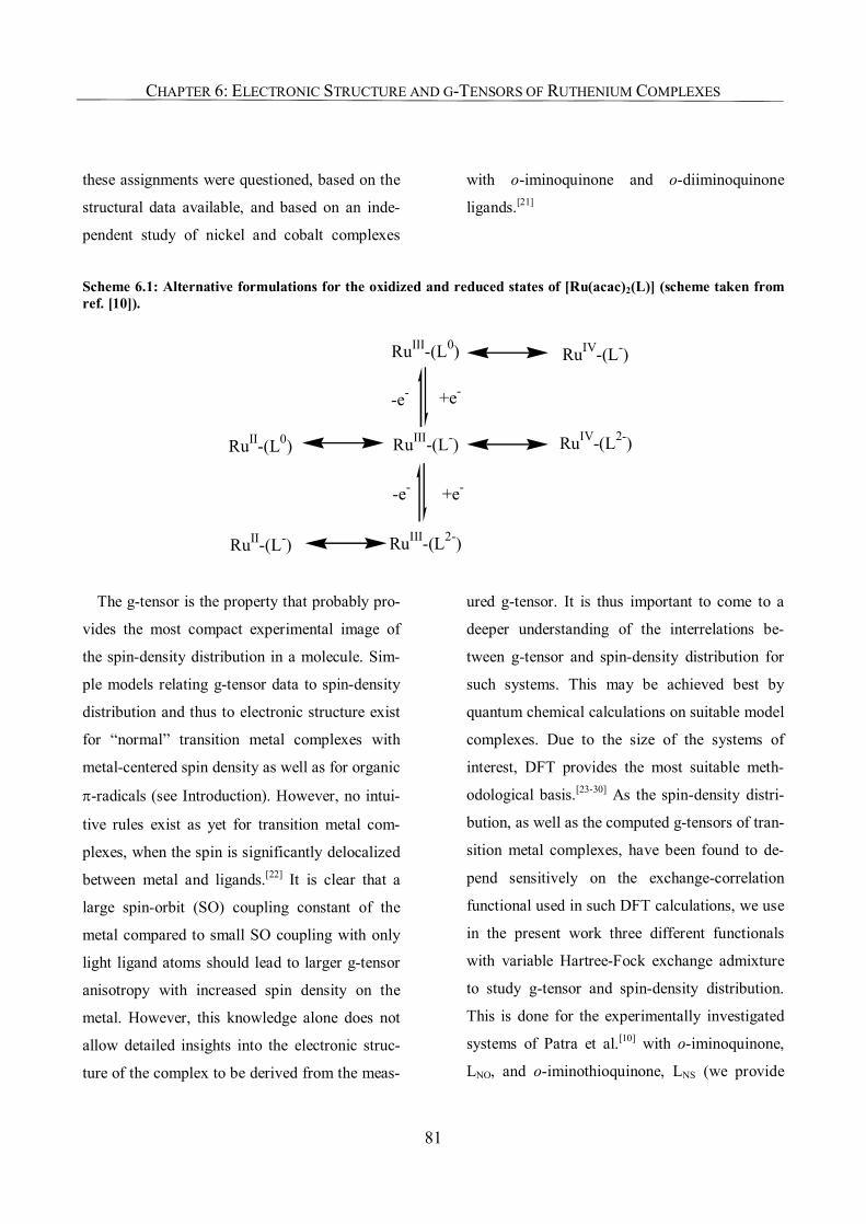
CHAPTER 6: ELECTRONIC STRUCTURE AND G-TENSORS OF RUTHENIUM COMPLEXES
81
these assignments were questioned, based on the
structural data available, and based on an inde-
pendent study of nickel and cobalt complexes
with o-iminoquinone and o-diiminoquinone
ligands.[21]
Scheme 6.1: Alternative formulations for the oxidized and reduced states of [Ru(acac)2(L)] (scheme taken from ref. [10]).
The g-tensor is the property that probably pro-
vides the most compact experimental image of
the spin-density distribution in a molecule. Sim-
ple models relating g-tensor data to spin-density
distribution and thus to electronic structure exist
for “normal” transition metal complexes with
metal-centered spin density as well as for organic
π-radicals (see Introduction). However, no intui-
tive rules exist as yet for transition metal com-
plexes, when the spin is significantly delocalized
between metal and ligands.[22] It is clear that a
large spin-orbit (SO) coupling constant of the
metal compared to small SO coupling with only
light ligand atoms should lead to larger g-tensor
anisotropy with increased spin density on the
metal. However, this knowledge alone does not
allow detailed insights into the electronic struc-
ture of the complex to be derived from the meas-
ured g-tensor. It is thus important to come to a
deeper understanding of the interrelations be-
tween g-tensor and spin-density distribution for
such systems. This may be achieved best by
quantum chemical calculations on suitable model
complexes. Due to the size of the systems of
interest, DFT provides the most suitable meth-
odological basis.[23-30] As the spin-density distri-
bution, as well as the computed g-tensors of tran-
sition metal complexes, have been found to de-
pend sensitively on the exchange-correlation
functional used in such DFT calculations, we use
in the present work three different functionals
with variable Hartree-Fock exchange admixture
to study g-tensor and spin-density distribution.
This is done for the experimentally investigated
systems of Patra et al.[10] with o-iminoquinone,
LNO, and o-iminothioquinone, LNS (we provide
RuIII-(L0)
RuIII-(L2-)
RuIII-(L-) RuIV-(L2-)
RuIV-(L-)
RuII-(L0)
RuII-(L-)
-e- +e-
+e--e-
CHAPTER 6: ELECTRONIC STRUCTURE AND G-TENSORS OF RUTHENIUM COMPLEXES
82
also a study of the two neutral complexes), as
well as for the as yet not studied analogues with
symmetrical o-quinone (LOO; related to ben-
zenediolato), o-diiminoquinone (LNN; related to
o-phenylenediamine), and o-dithioquinone (LSS;
related to benzenedithiolato) ligands.
As the combination of analysis methods em-
ployed provides an unprecedentedly detailed
picture of charge and spin-density distributions
for the different charge states of the title com-
plexes, rather general conclusions may be drawn
on the interrelations between structure, spectros-
copy, and electronic structure of complexes with
o-quinonoid ligands.
6.2. Computational Details
All structure optimizations employed the Tur-
bomole 5.6 program,[31] at unrestricted Kohn-
Sham (UKS) level. A quasirelativistic small-core
ECP[32] and a [7s6p5d]/(5s3p2d) valence basis
set[33] were used for Ru, together with DZVP all-
electron basis sets[34] for C, N, O, S, and H. Ex-
change-correlation functionals to be compared
are the BP86 generalized gradient approximation
(GGA),[35, 36] as well as the hybrid B3LYP[37, 38]
and BHLYP[39, 40] functionals. This sequence
corresponds to 0%, ca. 20%, and 50% Hartree-
Fock exchange admixture, respectively. For the
BP86 GGA functional, the Coulomb term was
evaluated by density fitting (RI-DFT method),
with SVP auxiliary basis sets.[41]
Calculation of the g-tensor was done in each
case using the structure and Kohn-Sham wave
function for a given functional, as obtained from
the structure optimizations above. The unre-
stricted Kohn-Sham orbitals were transferred by
suitable interface routines to the in-house MAG-
ReSpect property package,[42] which was used for
the g-tensor calculations. A common gauge ori-
gin at the metal nucleus was employed. The SO
operator was made up from an accurate and effi-
cient superposition[25, 29] of a spin-orbit pseudopo-
tential on Ru[32] and all-electron Breit-Pauli
atomic mean-field (AMFI)[43, 44] SO operators for
the ligand atoms.
Natural atomic charges[45] from Natural Popu-
lation Analyses (NPA) were obtained with a
standalone version of the NBO4.M program,[46]
interfaced to Turbomole in our group.[47] NPA
and Mulliken[48] spin densities were found to be
very similar. We will refer to Mulliken spin den-
sities, as it was easier to access them for individ-
ual MOs. Molecular structures, canonical and
natural orbitals, and spin density isosurfaces are
displayed with the Molekel 4.3 program.[49] To
analyze canonical MOs in strongly spin-
polarized Kohn-Sham wave functions, we have
employed overlap criteria to identify the corre-
sponding spin-up and spin-down component
belonging to a given formally doubly occupied
MO.[50]
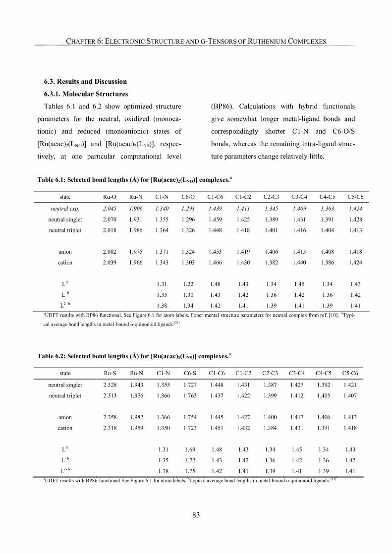
CHAPTER 6: ELECTRONIC STRUCTURE AND G-TENSORS OF RUTHENIUM COMPLEXES
83
6.3. Results and Discussion
6.3.1. Molecular Structures
Tables 6.1 and 6.2 show optimized structure
parameters for the neutral, oxidized (monoca-
tionic) and reduced (monoanionic) states of
[Ru(acac)2(LNO)] and [Ru(acac)2(LNS)], respec-
tively, at one particular computational level
(BP86). Calculations with hybrid functionals
give somewhat longer metal-ligand bonds and
correspondingly shorter C1-N and C6-O/S
bonds, whereas the remaining intra-ligand struc-
ture parameters change relatively little.
Table 6.1: Selected bond lengths (Å) for [Ru(acac)2(LNO)] complexes.a
state Ru-O Ru-N C1-N C6-O C1-C6 C1-C2 C2-C3 C3-C4 C4-C5 C5-C6
neutral exp. 2.045 1.906 1.340 1.291 1.439 1.411 1.345 1.409 1.363 1.424
neutral singlet 2.070 1.931 1.355 1.296 1.459 1.425 1.389 1.431 1.391 1.428
neutral triplet 2.018 1.986 1.364 1.326 1.448 1.418 1.401 1.416 1.404 1.413
anion 2.082 1.975 1.371 1.324 1.453 1.419 1.406 1.415 1.408 1.418
cation 2.039 1.966 1.343 1.303 1.466 1.430 1.382 1.440 1.386 1.424
L b
1.31 1.22 1.48 1.43 1.34 1.45 1.34 1.43
L- b 1.35 1.30 1.43 1.42 1.36 1.42 1.36 1.42
L2- b 1.38 1.34 1.42 1.41 1.39 1.41 1.39 1.41 aUDFT results with BP86 functional. See Figure 6.1 for atom labels. Experimental structure parameters for neutral complex from ref. [10]. bTypi-
cal average bond lengths in metal-bound o-quinonoid ligands.[51]
Table 6.2: Selected bond lengths (Å) for [Ru(acac)2(LNS)] complexes.a
state Ru-S Ru-N C1-N C6-S C1-C6 C1-C2 C2-C3 C3-C4 C4-C5 C5-C6
neutral singlet 2.328 1.943 1.355 1.727 1.448 1.431 1.387 1.427 1.392 1.421
neutral triplet 2.313 1.976 1.366 1.763 1.437 1.422 1.399 1.412 1.405 1.407
anion 2.358 1.982 1.366 1.754 1.445 1.427 1.400 1.417 1.406 1.413
cation 2.318 1.959 1.350 1.723 1.451 1.432 1.384 1.431 1.391 1.418
L b
1.31 1.69 1.48 1.43 1.34 1.45 1.34 1.43
L- b 1.35 1.72 1.43 1.42 1.36 1.42 1.36 1.42
L2- b 1.38 1.75 1.42 1.41 1.39 1.41 1.39 1.41 aUDFT results with BP86 functional See Figure 6.1 for atom labels. bTypical average bond lengths in metal-bound o-quinonoid ligands. [51]
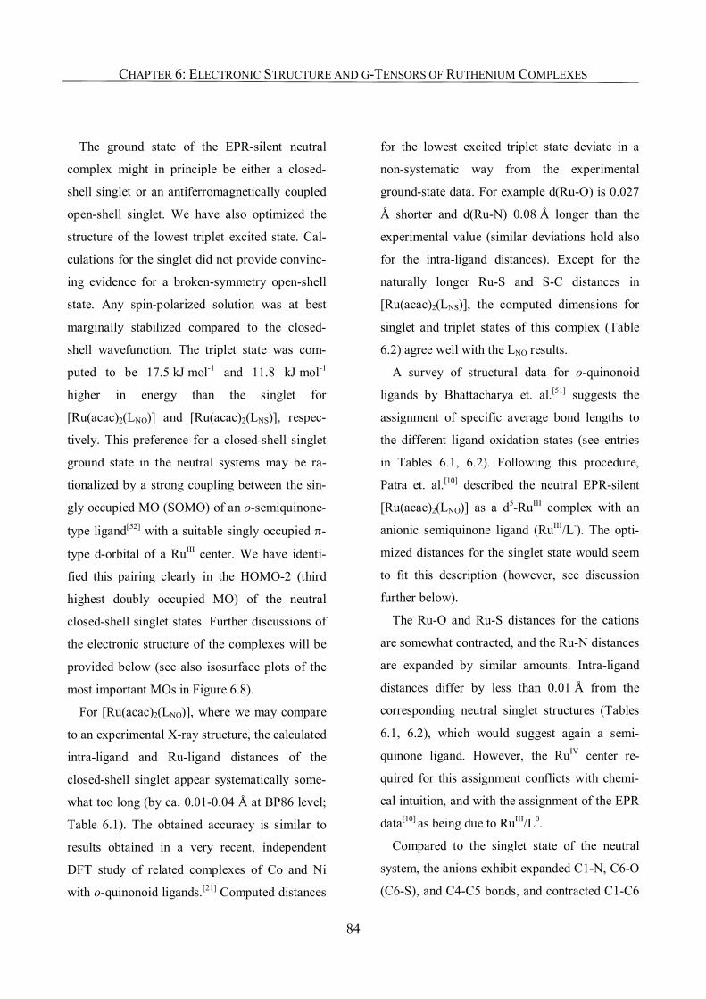
CHAPTER 6: ELECTRONIC STRUCTURE AND G-TENSORS OF RUTHENIUM COMPLEXES
84
The ground state of the EPR-silent neutral
complex might in principle be either a closed-
shell singlet or an antiferromagnetically coupled
open-shell singlet. We have also optimized the
structure of the lowest triplet excited state. Cal-
culations for the singlet did not provide convinc-
ing evidence for a broken-symmetry open-shell
state. Any spin-polarized solution was at best
marginally stabilized compared to the closed-
shell wavefunction. The triplet state was com-
puted to be 17.5 kJ mol-1 and 11.8 kJ mol-1
higher in energy than the singlet for
[Ru(acac)2(LNO)] and [Ru(acac)2(LNS)], respec-
tively. This preference for a closed-shell singlet
ground state in the neutral systems may be ra-
tionalized by a strong coupling between the sin-
gly occupied MO (SOMO) of an o-semiquinone-
type ligand[52] with a suitable singly occupied π-
type d-orbital of a RuIII center. We have identi-
fied this pairing clearly in the HOMO-2 (third
highest doubly occupied MO) of the neutral
closed-shell singlet states. Further discussions of
the electronic structure of the complexes will be
provided below (see also isosurface plots of the
most important MOs in Figure 6.8).
For [Ru(acac)2(LNO)], where we may compare
to an experimental X-ray structure, the calculated
intra-ligand and Ru-ligand distances of the
closed-shell singlet appear systematically some-
what too long (by ca. 0.01-0.04 Å at BP86 level;
Table 6.1). The obtained accuracy is similar to
results obtained in a very recent, independent
DFT study of related complexes of Co and Ni
with o-quinonoid ligands.[21] Computed distances
for the lowest excited triplet state deviate in a
non-systematic way from the experimental
ground-state data. For example d(Ru-O) is 0.027
Å shorter and d(Ru-N) 0.08 Å longer than the
experimental value (similar deviations hold also
for the intra-ligand distances). Except for the
naturally longer Ru-S and S-C distances in
[Ru(acac)2(LNS)], the computed dimensions for
singlet and triplet states of this complex (Table
6.2) agree well with the LNO results.
A survey of structural data for o-quinonoid
ligands by Bhattacharya et. al.[51] suggests the
assignment of specific average bond lengths to
the different ligand oxidation states (see entries
in Tables 6.1, 6.2). Following this procedure,
Patra et. al.[10] described the neutral EPR-silent
[Ru(acac)2(LNO)] as a d5-RuIII complex with an
anionic semiquinone ligand (RuIII/L-). The opti-
mized distances for the singlet state would seem
to fit this description (however, see discussion
further below).
The Ru-O and Ru-S distances for the cations
are somewhat contracted, and the Ru-N distances
are expanded by similar amounts. Intra-ligand
distances differ by less than 0.01 Å from the
corresponding neutral singlet structures (Tables
6.1, 6.2), which would suggest again a semi-
quinone ligand. However, the RuIV center re-
quired for this assignment conflicts with chemi-
cal intuition, and with the assignment of the EPR
data[10] as being due to RuIII/L0.
Compared to the singlet state of the neutral
system, the anions exhibit expanded C1-N, C6-O
(C6-S), and C4-C5 bonds, and contracted C1-C6
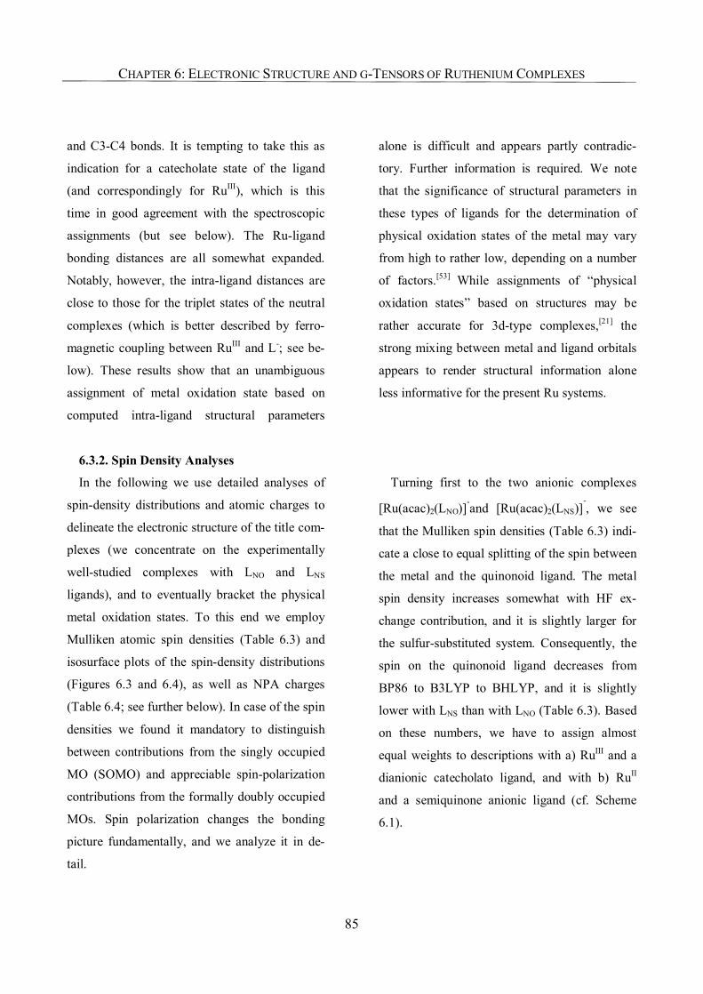
CHAPTER 6: ELECTRONIC STRUCTURE AND G-TENSORS OF RUTHENIUM COMPLEXES
85
and C3-C4 bonds. It is tempting to take this as
indication for a catecholate state of the ligand
(and correspondingly for RuIII), which is this
time in good agreement with the spectroscopic
assignments (but see below). The Ru-ligand
bonding distances are all somewhat expanded.
Notably, however, the intra-ligand distances are
close to those for the triplet states of the neutral
complexes (which is better described by ferro-
magnetic coupling between RuIII and L-; see be-
low). These results show that an unambiguous
assignment of metal oxidation state based on
computed intra-ligand structural parameters
alone is difficult and appears partly contradic-
tory. Further information is required. We note
that the significance of structural parameters in
these types of ligands for the determination of
physical oxidation states of the metal may vary
from high to rather low, depending on a number
of factors.[53] While assignments of “physical
oxidation states” based on structures may be
rather accurate for 3d-type complexes,[21] the
strong mixing between metal and ligand orbitals
appears to render structural information alone
less informative for the present Ru systems.
6.3.2. Spin Density Analyses
In the following we use detailed analyses of
spin-density distributions and atomic charges to
delineate the electronic structure of the title com-
plexes (we concentrate on the experimentally
well-studied complexes with LNO and LNS
ligands), and to eventually bracket the physical
metal oxidation states. To this end we employ
Mulliken atomic spin densities (Table 6.3) and
isosurface plots of the spin-density distributions
(Figures 6.3 and 6.4), as well as NPA charges
(Table 6.4; see further below). In case of the spin
densities we found it mandatory to distinguish
between contributions from the singly occupied
MO (SOMO) and appreciable spin-polarization
contributions from the formally doubly occupied
MOs. Spin polarization changes the bonding
picture fundamentally, and we analyze it in de-
tail.
Turning first to the two anionic complexes
[Ru(acac)2(LNO)]-and [Ru(acac)2(LNS)]-, we see
that the Mulliken spin densities (Table 6.3) indi-
cate a close to equal splitting of the spin between
the metal and the quinonoid ligand. The metal
spin density increases somewhat with HF ex-
change contribution, and it is slightly larger for
the sulfur-substituted system. Consequently, the
spin on the quinonoid ligand decreases from
BP86 to B3LYP to BHLYP, and it is slightly
lower with LNS than with LNO (Table 6.3). Based
on these numbers, we have to assign almost
equal weights to descriptions with a) RuIII and a
dianionic catecholato ligand, and with b) RuII
and a semiquinone anionic ligand (cf. Scheme
6.1).
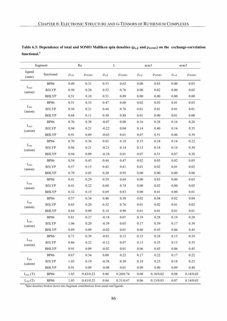
CHAPTER 6: ELECTRONIC STRUCTURE AND G-TENSORS OF RUTHENIUM COMPLEXES
86
Table 6.3: Dependence of total and SOMO Mulliken spin densities (ρα-β and ρSOMO) on the exchange-correlation
functional.a
fragment: Ru L acac1 acac2
ligand (state)
functional ρα-β ρSOMO ρα-β ρSOMO ρα-β ρSOMO ρα-β ρSOMO
BP86 0.49 0.31 0.53 0.62 0.00 0.03 0.00 0.03
B3LYP 0.50 0.20 0.52 0.76 0.00 0.02 0.00 0.02 LNO
(anion) BHLYP 0.51 0.10 0.51 0.89 0.00 0.00 0.00 0.00
BP86 0.51 0.33 0.47 0.60 0.02 0.03 0.01 0.03
B3LYP 0.56 0.21 0.44 0.76 0.01 0.01 0.01 0.01 LNS
(anion) BHLYP 0.68 0.11 0.30 0.88 0.01 0.00 0.01 0.00
BP86 0.76 0.38 -0.07 0.08 0.16 0.28 0.16 0.26
B3LYP 0.94 0.21 -0.22 0.04 0.14 0.40 0.14 0.35 LNO
(cation) BHLYP 0.91 0.09 -0.03 0.01 0.07 0.51 0.06 0.39
BP86 0.70 0.36 0.03 0.18 0.15 0.24 0.14 0.22
B3LYP 0.94 0.21 -0.21 0.14 0.13 0.34 0.14 0.30 LNS
(cation) BHLYP 0.94 0.09 -0.10 0.01 0.07 0.51 0.07 0.38
BP86 0.54 0.43 0.44 0.47 0.02 0.05 0.02 0.05
B3LYP 0.57 0.15 0.42 0.81 0.01 0.02 0.01 0.02 LOO
(anion) BHLYP 0.79 0.05 0.20 0.95 0.00 0.00 0.00 0.00
BP86 0.41 0.29 0.59 0.64 0.00 0.03 0.00 0.03
B3LYP 0.41 0.22 0.60 0.74 0.00 0.02 0.00 0.02 LNN
(anion) BHLYP 0.32 0.15 0.69 0.83 0.00 0.01 0.00 0.01
BP86 0.57 0.34 0.40 0.58 0.02 0.04 0.02 0.04
B3LYP 0.65 0.20 0.32 0.76 0.01 0.02 0.01 0.02 LSS
(anion) BHLYP 0.84 0.09 0.14 0.90 0.01 0.01 0.01 0.01
BP86 0.81 0.37 -0.18 0.07 0.19 0.28 0.19 0.28
B3LYP 1.06 0.20 -0.39 0.03 0.17 0.39 0.17 0.39 LOO
(cation) BHLYP 0.89 0.09 -0.02 0.01 0.06 0.45 0.06 0.45
BP86 0.71 0.39 -0.01 0.13 0.15 0.24 0.15 0.24
B3LYP 0.86 0.22 -0.12 0.07 0.13 0.35 0.13 0.35 LNN
(cation) BHLYP 0.91 0.09 -0.02 0.01 0.06 0.45 0.06 0.45
BP86 0.67 0.34 0.00 0.22 0.17 0.22 0.17 0.22
B3LYP 1.03 0.19 -0.38 0.30 0.18 0.25 0.18 0.25 LSS
(cation) BHLYP 0.91 0.09 -0.08 0.01 0.09 0.40 0.09 0.40
LNO (T) BP86 1.03 0.43/0.22 0.80 0.20/0.74 0.08 0.18/0.02 0.08 0.18/0.02
LNS (T) BP86 1.03 0.41/0.25 0.84 0.31/0.67 0.06 0.13/0.03 0.07 0.14/0.03 aSpin densities broken down into fragment contributions from metal and ligands.
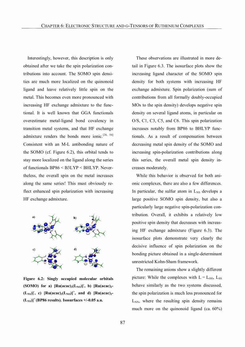
CHAPTER 6: ELECTRONIC STRUCTURE AND G-TENSORS OF RUTHENIUM COMPLEXES
87
Interestingly, however, this description is only
obtained after we take the spin polarization con-
tributions into account. The SOMO spin densi-
ties are much more localized on the quinonoid
ligand and leave relatively little spin on the
metal. This becomes even more pronounced with
increasing HF exchange admixture to the func-
tional. It is well known that GGA functionals
overestimate metal-ligand bond covalency in
transition metal systems, and that HF exchange
admixture renders the bonds more ionic.[24, 54]
Consistent with an M-L antibonding nature of
the SOMO (cf. Figure 6.2), this orbital tends to
stay more localized on the ligand along the series
of functionals BP86 < B3LYP < BHLYP. Never-
theless, the overall spin on the metal increases
along the same series! This must obviously re-
flect enhanced spin polarization with increasing
HF exchange admixture.
Figure 6.2: Singly occupied molecular orbitals
(SOMO) for a) [Ru(acac)2(LNO)]-, b) [Ru(acac)2-
(LNS)]-, c) [Ru(acac)2(LNO)]+, and d) [Ru(acac)2-
(LNS)]+ (BP86 results). Isosurfaces +/-0.05 a.u.
These observations are illustrated in more de-
tail in Figure 6.3. The isosurface plots show the
increasing ligand character of the SOMO spin
density for both systems with increasing HF
exchange admixture. Spin polarization (sum of
contributions from all formally doubly-occupied
MOs to the spin density) develops negative spin
density on several ligand atoms, in particular on
O/S, C1, C3, C5, and C6. This spin polarization
increases notably from BP86 to BHLYP func-
tionals. As a result of compensation between
decreasing metal spin density of the SOMO and
increasing spin-polarization contributions along
this series, the overall metal spin density in-
creases moderately.
While this behavior is observed for both ani-
onic complexes, there are also a few differences.
In particular, the sulfur atom in LNS develops a
large positive SOMO spin density, but also a
particularly large negative spin-polarization con-
tribution. Overall, it exhibits a relatively low
positive spin density that decreases with increas-
ing HF exchange admixture (Figure 6.3). The
isosurface plots demonstrate very clearly the
decisive influence of spin polarization on the
bonding picture obtained in a single-determinant
unrestricted Kohn-Sham framework.
The remaining anions show a slightly different
picture: While the complexes with L = LOO, LSS
behave similarly as the two systems discussed,
the spin polarization is much less pronounced for
LNN, where the resulting spin density remains
much more on the quinonoid ligand (ca. 60%)
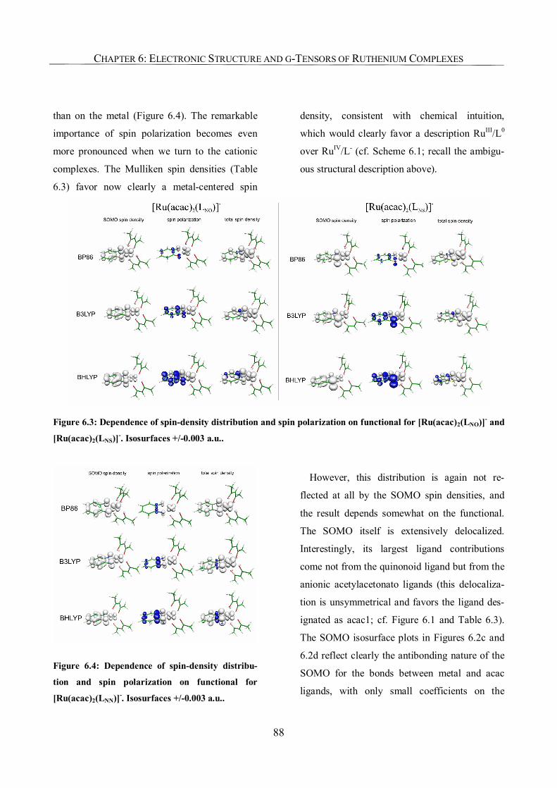
CHAPTER 6: ELECTRONIC STRUCTURE AND G-TENSORS OF RUTHENIUM COMPLEXES
88
than on the metal (Figure 6.4). The remarkable
importance of spin polarization becomes even
more pronounced when we turn to the cationic
complexes. The Mulliken spin densities (Table
6.3) favor now clearly a metal-centered spin
density, consistent with chemical intuition,
which would clearly favor a description RuIII/L0
over RuIV/L- (cf. Scheme 6.1; recall the ambigu-
ous structural description above).
Figure 6.3: Dependence of spin-density distribution and spin polarization on functional for [Ru(acac)2(LNO)]- and
[Ru(acac)2(LNS)]-. Isosurfaces +/-0.003 a.u..
Figure 6.4: Dependence of spin-density distribu-
tion and spin polarization on functional for
[Ru(acac)2(LNN)]-. Isosurfaces +/-0.003 a.u..
However, this distribution is again not re-
flected at all by the SOMO spin densities, and
the result depends somewhat on the functional.
The SOMO itself is extensively delocalized.
Interestingly, its largest ligand contributions
come not from the quinonoid ligand but from the
anionic acetylacetonato ligands (this delocaliza-
tion is unsymmetrical and favors the ligand des-
ignated as acac1; cf. Figure 6.1 and Table 6.3).
The SOMO isosurface plots in Figures 6.2c and
6.2d reflect clearly the antibonding nature of the
SOMO for the bonds between metal and acac
ligands, with only small coefficients on the
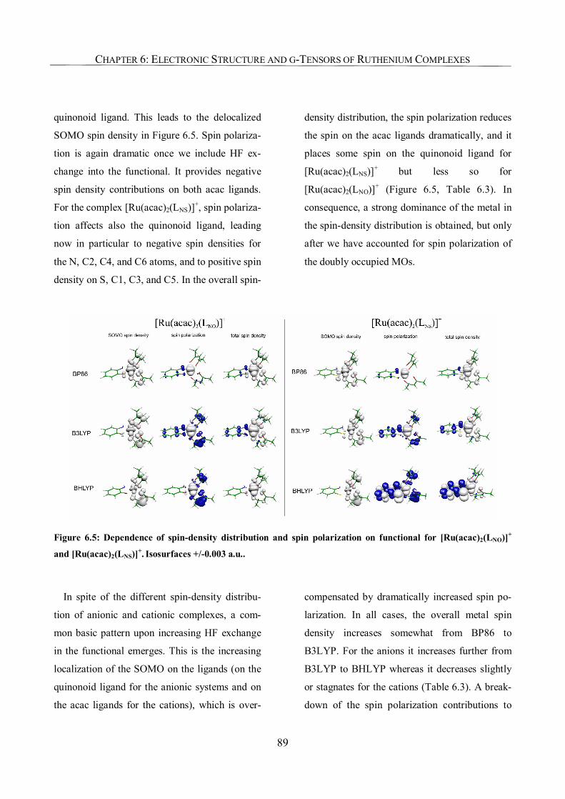
CHAPTER 6: ELECTRONIC STRUCTURE AND G-TENSORS OF RUTHENIUM COMPLEXES
89
quinonoid ligand. This leads to the delocalized
SOMO spin density in Figure 6.5. Spin polariza-
tion is again dramatic once we include HF ex-
change into the functional. It provides negative
spin density contributions on both acac ligands.
For the complex [Ru(acac)2(LNS)]+, spin polariza-
tion affects also the quinonoid ligand, leading
now in particular to negative spin densities for
the N, C2, C4, and C6 atoms, and to positive spin
density on S, C1, C3, and C5. In the overall spin-
density distribution, the spin polarization reduces
the spin on the acac ligands dramatically, and it
places some spin on the quinonoid ligand for
[Ru(acac)2(LNS)]+ but less so for
[Ru(acac)2(LNO)]+ (Figure 6.5, Table 6.3). In
consequence, a strong dominance of the metal in
the spin-density distribution is obtained, but only
after we have accounted for spin polarization of
the doubly occupied MOs.
Figure 6.5: Dependence of spin-density distribution and spin polarization on functional for [Ru(acac)2(LNO)]+
and [Ru(acac)2(LNS)]+. Isosurfaces +/-0.003 a.u..
In spite of the different spin-density distribu-
tion of anionic and cationic complexes, a com-
mon basic pattern upon increasing HF exchange
in the functional emerges. This is the increasing
localization of the SOMO on the ligands (on the
quinonoid ligand for the anionic systems and on
the acac ligands for the cations), which is over-
compensated by dramatically increased spin po-
larization. In all cases, the overall metal spin
density increases somewhat from BP86 to
B3LYP. For the anions it increases further from
B3LYP to BHLYP whereas it decreases slightly
or stagnates for the cations (Table 6.3). A break-
down of the spin polarization contributions to
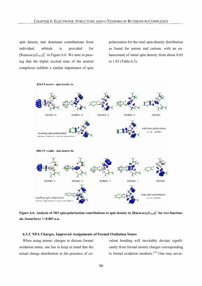
CHAPTER 6: ELECTRONIC STRUCTURE AND G-TENSORS OF RUTHENIUM COMPLEXES
90
spin density into dominant contributions from
individual orbitals is provided for
[Ru(acac)2(LNO)]+ in Figure 6.6. We note in pass-
ing that the triplet excited state of the neutral
complexes exhibits a similar importance of spin
polarization for the total spin-density distribution
as found for anions and cations, with an en-
hancement of metal spin density from about 0.65
to 1.03 (Table 6.3).
Figure 6.6: Analysis of MO spin-polarization contributions to spin density in [Ru(acac)2(LNO)]+ for two function-
als. Isosurfaces +/-0.003 a.u..
6.3.3. NPA Charges, Improved Assignments of Formal Oxidation States
When using atomic charges to discuss formal
oxidation states, one has to keep in mind that the
actual charge distribution in the presence of co-
valent bonding will inevitably deviate signifi-
cantly from formal atomic charges corresponding
to formal oxidation numbers.[55] One may never-
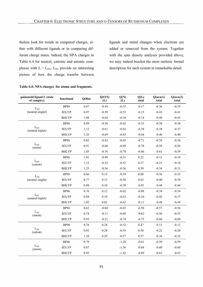
CHAPTER 6: ELECTRONIC STRUCTURE AND G-TENSORS OF RUTHENIUM COMPLEXES
91
theless look for trends in computed charges, ei-
ther with different ligands or in comparing dif-
ferent charge states. Indeed, the NPA charges in
Table 6.4 for neutral, cationic and anionic com-
plexes with L = LNO, LNS provide an interesting
picture of how the charge transfer between
ligands and metal changes when electrons are
added or removed from the system. Together
with the spin density analyses provided above,
we may indeed bracket the most realistic formal
description for each system in remarkable detail.
Table 6.4: NPA charges for atoms and fragments.
quinonoid ligand L (state of complex) functional Q(Ru) Q(O/S)
(L) Q(N) (L)
Q(L) total
Q(acac1) total
Q(acac2) total
BP86 0.87 -0.54 -0.53 -0.17 -0.36 -0.35
B3LYP 0.97 -0.59 -0.53 -0.15 -0.43 -0.41 LNO
(neutral singlet)
BHLYP 1.08 -0.64 -0.54 -0.14 -0.49 -0.45
BP86 0.99 -0.56 -0.62 -0.33 -0.38 -0.38
B3LYP 1.12 -0.61 -0.63 -0.38 -0.38 -0.37 LNO (neutral triplet)
BHLYP 1.26 -0.69 -0.63 -0.44 -0.40 -0.40
BP86 0.82 -0.62 -0.65 -0.71 -0.56 -0.54
B3LYP 0.91 -0.68 -0.68 -0.78 -0.58 -0.56 LNO (anion)
BHLYP 1.05 -0.76 -0.70 -0.86 -0.61 -0.59
BP86 1.01 -0.49 -0.51 0.22 -0.12 -0.10
B3LYP 1.12 -0.52 -0.53 0.27 -0.21 -0.18 LNO (cation)
BHLYP 1.25 -0.56 -0.56 0.39 -0.34 -0.31
BP86 0.66 0.15 -0.54 0.06 -0.36 -0.35
B3LYP 0.77 0.13 -0.56 0.02 -0.40 -0.39 LNS
(neutral singlet)
BHLYP 0.88 0.10 -0.58 -0.01 -0.44 -0.44
BP86 0.76 0.12 -0.62 -0.08 -0.34 -0.34
B3LYP 0.88 0.10 -0.63 -0.10 -0.42 -0.37 LNS (neutral triplet)
BHLYP 1.02 0.02 -0.63 -0.11 -0.48 -0.44
BP86 0.62 -0.04 -0.65 -0.50 -0.57 -0.56
B3LYP 0.74 -0.11 -0.68 -0.62 -0.56 -0.55 LNS (anion)
BHLYP 0.93 -0.21 -0.74 -0.75 -0.60 -0.60
BP86 0.78 0.28 -0.52 0.47 -0.13 -0.12
B3LYP 0.92 0.28 -0.55 0.50 -0.22 -0.20 LNS (cation)
BHLYP 1.10 0.29 -0.57 0.57 -0.36 -0.32
BP86 0.79 -1.28 -0.61 -0.59 -0.59
B3LYP 0.87 -1.36 -0.68 -0.60 -0.60 LNN (anion)
BHLYP 0.95 -1.42 -0.69 -0.63 -0.63
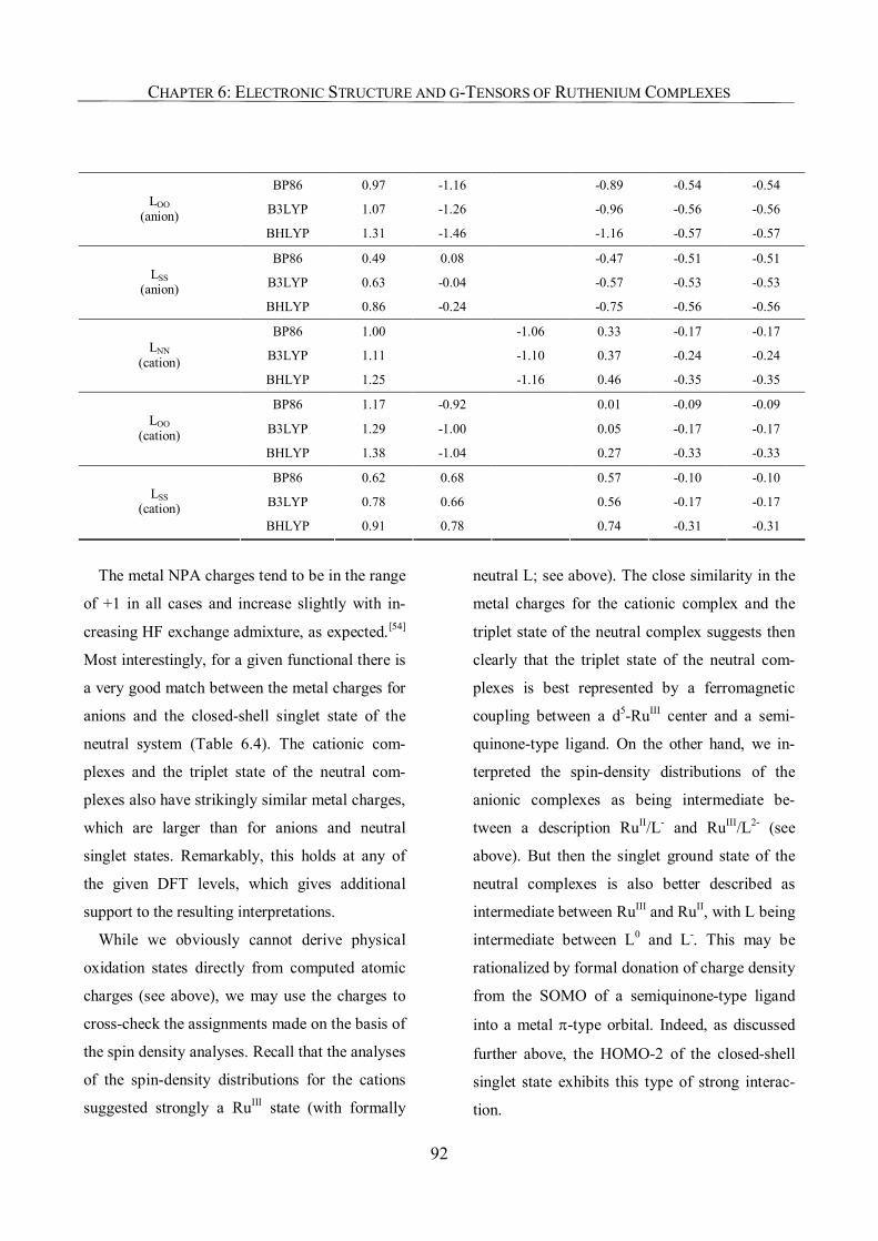
CHAPTER 6: ELECTRONIC STRUCTURE AND G-TENSORS OF RUTHENIUM COMPLEXES
92
BP86 0.97 -1.16 -0.89 -0.54 -0.54
B3LYP 1.07 -1.26 -0.96 -0.56 -0.56 LOO (anion)
BHLYP 1.31 -1.46 -1.16 -0.57 -0.57
BP86 0.49 0.08 -0.47 -0.51 -0.51
B3LYP 0.63 -0.04 -0.57 -0.53 -0.53 LSS (anion)
BHLYP 0.86 -0.24 -0.75 -0.56 -0.56
BP86 1.00 -1.06 0.33 -0.17 -0.17
B3LYP 1.11 -1.10 0.37 -0.24 -0.24 LNN (cation)
BHLYP 1.25 -1.16 0.46 -0.35 -0.35
BP86 1.17 -0.92 0.01 -0.09 -0.09
B3LYP 1.29 -1.00 0.05 -0.17 -0.17 LOO (cation)
BHLYP 1.38 -1.04 0.27 -0.33 -0.33
BP86 0.62 0.68 0.57 -0.10 -0.10
B3LYP 0.78 0.66 0.56 -0.17 -0.17 LSS (cation)
BHLYP 0.91 0.78 0.74 -0.31 -0.31
The metal NPA charges tend to be in the range
of +1 in all cases and increase slightly with in-
creasing HF exchange admixture, as expected.[54]
Most interestingly, for a given functional there is
a very good match between the metal charges for
anions and the closed-shell singlet state of the
neutral system (Table 6.4). The cationic com-
plexes and the triplet state of the neutral com-
plexes also have strikingly similar metal charges,
which are larger than for anions and neutral
singlet states. Remarkably, this holds at any of
the given DFT levels, which gives additional
support to the resulting interpretations.
While we obviously cannot derive physical
oxidation states directly from computed atomic
charges (see above), we may use the charges to
cross-check the assignments made on the basis of
the spin density analyses. Recall that the analyses
of the spin-density distributions for the cations
suggested strongly a RuIII state (with formally
neutral L; see above). The close similarity in the
metal charges for the cationic complex and the
triplet state of the neutral complex suggests then
clearly that the triplet state of the neutral com-
plexes is best represented by a ferromagnetic
coupling between a d5-RuIII center and a semi-
quinone-type ligand. On the other hand, we in-
terpreted the spin-density distributions of the
anionic complexes as being intermediate be-
tween a description RuII/L- and RuIII/L2- (see
above). But then the singlet ground state of the
neutral complexes is also better described as
intermediate between RuIII and RuII, with L being
intermediate between L0 and L-. This may be
rationalized by formal donation of charge density
from the SOMO of a semiquinone-type ligand
into a metal π-type orbital. Indeed, as discussed
further above, the HOMO-2 of the closed-shell
singlet state exhibits this type of strong interac-
tion.
CHAPTER 6: ELECTRONIC STRUCTURE AND G-TENSORS OF RUTHENIUM COMPLEXES
93
The ligand fragment NPA charges (Table 6.4)
confirm our reasoning: The charge on L is most
negative for the anionic complexes, where the
ligand is thought to be intermediate between L-
and L2-. It is somewhat less negative for the trip-
let state of the neutral system, where we assign
the ligand as close to L-. The still lower value for
the closed-shell singlet corresponds to our de-
scription of L as intermediate between L0 and L-.
Finally, the slightly positive ligand charge on L
for the cationic complexes reflects nicely the
assignment as L0. In all cases, the charge on LNS
is less negative (more positive) than on LNO,
consistent with the lower electronegativity of
sulfur compared to oxygen (see also individual
charges for the ligand donor atoms in Table 6.4;
the appreciable Ru-S covalency is relevant for
the discussion of spin contamination further be-
low). Charges on the acac ligands are generally
negative and vary more moderately than on L,
consistent with a buffer-type role of these ani-
onic co-ligands. Obviously, the covalency of the
metal-acac interactions is least pronounced for
the anionic complexes and most pronounced for
the cations. NPA charges for complexes with the
other ligands provide a similar picture.
Based on these detailed analyses of spin and
charge densities, we therefore have to modify the
established interrelations between intramolecular
distances and charge state of o-quinonoid
ligands.[10, 51] This holds for the systems studied
here, but probably also for many other related
complexes. Recall that the X-ray structure of
neutral [Ru(acac)2(LNO)] was interpreted as re-
flecting a RuIII/L- system.[10] Both experimental
and computed intra-ligand distances for the
closed-shell singlet ground state agreed well with
the tabulated data[51] for o-quinonoid ligands in
an L- monoanionic state. However, our present
analyses for the closed-shell singlet suggest a
description intermediate between L- and L0. It is
rather the triplet state of the neutral complexes
that corresponds to a relatively clearcut RuIII/L-
description (see above). We suggest therefore
that, after correction for a slight systematic over-
estimate of distances by the DFT level used (see
above), the computed intra-ligand distances for
the triplet states in Tables 6.1 and 6.2 should
provide a better estimate for metal-bound o-
quinonoid ligands in a semiquinone state. Simi-
larly, the cationic complexes should provide
reasonable reference values for a neutral state of
the bound ligands (Table 6.1, 6.2).
6.3.4. g-Tensor Values and Orientations
Table 6.5 compares computed g-tensors with
the three different density functionals for all five
cationic and five anionic complexes, together
with the available experimental results for the
iminoquinone and iminothioquinone complexes.
We provide also for each of the three functionals
employed the <S2> expectation value of the
Kohn-Sham determinant as an approximate
CHAPTER 6: ELECTRONIC STRUCTURE AND G-TENSORS OF RUTHENIUM COMPLEXES
94
measure of spin contamination.[56,57] All four
experimentally determined g-tensors exhibit one
component significantly below ge (g11) and two
components appreciably above ge (Table 6.5).
The latter (g22, g33) have either been reported as
equal (for [Ru(acac)2(LNO)]- and for
[Ru(acac)2(LNS)]+), leading to an axially symmet-
rical tensor, or as different (for [Ru(acac)2(LNO)]+
and for [Ru(acac)2(LNS)]-), leading to a rhombic
tensor. In all four examples, the experimentally
determined g-tensor anisotropy g33-g11 is size-
able, between 191 ppt and 305 ppt. The isotropic
g-values are all above ge, but more so for the
cationic than for the anionic complexes.
The computed g-tensors (Table 6.5) exhibit a
pronounced dependence on the Hartree-Fock
exchange admixture to the exchange-correlation
functional. Let us start with the experimentally
negative g-shift component, ∆g11. This is not
reproduced at all very well by the calculations.
The gradient-corrected BP86 functional provides
small negative ∆g11 for the anions or small posi-
tive ∆g11 for the cations. Admixture of ca. 20%
HF exchange with the B3LYP functional im-
proves agreement with experimental ∆g11 some-
what for the two anionic complexes but leads to
even slightly more positive ∆g11 for the two cati-
onic complexes. Only upon increasing the HF
exchange admixture to 50% with the BHLYP
functional, ∆g11 is computed to be negative also
for the cations. But it remains appreciably (30-
70 ppt) above experiment. While this component
is thus rather sensitive to the exchange-
correlation functional, we believe that the devia-
tions from experiment reflect in particular the
neglect of higher-order relativistic contributions
in our present calculations (some of the scalar
relativistic effects are included via the Ru ECP).
In σ-radicals containing heavy elements, nega-
tive parallel g-shift components have been attrib-
uted either to higher-order SO effects (repro-
ducible in two-component calculations[58]) or to
cross-terms with scalar relativistic effects (in
Breit-Pauli perturbation analyses[59]). Ligand-
field arguments[60] attribute the negative ∆g|| in
low-spin d5 complexes partly to quadratic SO
contributions (as well as to couplings between
SOMO and “eg”-type orbitals,[61] cf. below).
Recent preliminary relativistic two-component
calculations on small tetragonal 4d-complexes
indicate indeed sizeable negative higher-order
SO contributions to g||.[63] Future two-component
analyses of the title complexes may provide
deeper insight into this as yet open question.
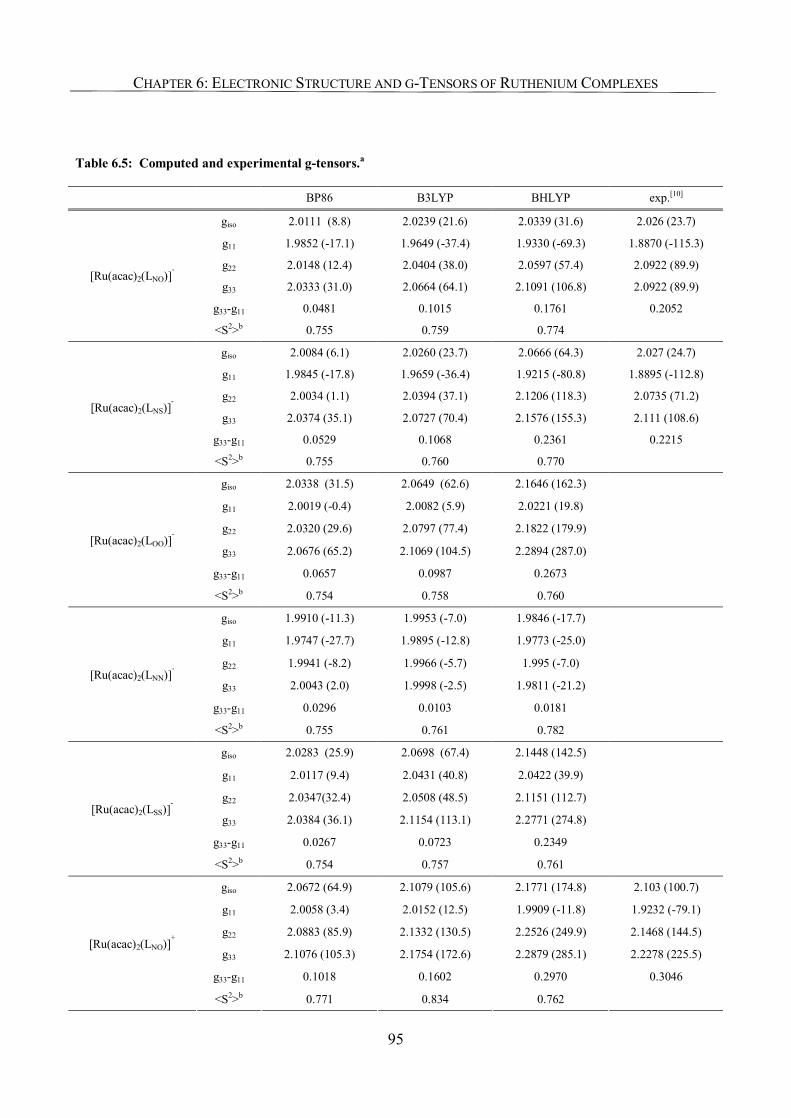
CHAPTER 6: ELECTRONIC STRUCTURE AND G-TENSORS OF RUTHENIUM COMPLEXES
95
Table 6.5: Computed and experimental g-tensors.a
BP86 B3LYP BHLYP exp.[10]
giso 2.0111 (8.8) 2.0239 (21.6) 2.0339 (31.6) 2.026 (23.7)
g11 1.9852 (-17.1) 1.9649 (-37.4) 1.9330 (-69.3) 1.8870 (-115.3)
g22 2.0148 (12.4) 2.0404 (38.0) 2.0597 (57.4) 2.0922 (89.9)
g33 2.0333 (31.0) 2.0664 (64.1) 2.1091 (106.8) 2.0922 (89.9)
g33-g11 0.0481 0.1015 0.1761 0.2052
[Ru(acac)2(LNO)]-
<S2>b 0.755 0.759 0.774
giso 2.0084 (6.1) 2.0260 (23.7) 2.0666 (64.3) 2.027 (24.7)
g11 1.9845 (-17.8) 1.9659 (-36.4) 1.9215 (-80.8) 1.8895 (-112.8)
g22 2.0034 (1.1) 2.0394 (37.1) 2.1206 (118.3) 2.0735 (71.2)
g33 2.0374 (35.1) 2.0727 (70.4) 2.1576 (155.3) 2.111 (108.6)
g33-g11 0.0529 0.1068 0.2361 0.2215
[Ru(acac)2(LNS)]-
<S2>b 0.755 0.760 0.770
giso 2.0338 (31.5) 2.0649 (62.6) 2.1646 (162.3)
g11 2.0019 (-0.4) 2.0082 (5.9) 2.0221 (19.8)
g22 2.0320 (29.6) 2.0797 (77.4) 2.1822 (179.9)
g33 2.0676 (65.2) 2.1069 (104.5) 2.2894 (287.0)
g33-g11 0.0657 0.0987 0.2673
[Ru(acac)2(LOO)]-
<S2>b 0.754 0.758 0.760
giso 1.9910 (-11.3) 1.9953 (-7.0) 1.9846 (-17.7)
g11 1.9747 (-27.7) 1.9895 (-12.8) 1.9773 (-25.0)
g22 1.9941 (-8.2) 1.9966 (-5.7) 1.995 (-7.0)
g33 2.0043 (2.0) 1.9998 (-2.5) 1.9811 (-21.2)
g33-g11 0.0296 0.0103 0.0181
[Ru(acac)2(LNN)]-
<S2>b 0.755 0.761 0.782
giso 2.0283 (25.9) 2.0698 (67.4) 2.1448 (142.5)
g11 2.0117 (9.4) 2.0431 (40.8) 2.0422 (39.9)
g22 2.0347(32.4) 2.0508 (48.5) 2.1151 (112.7)
g33 2.0384 (36.1) 2.1154 (113.1) 2.2771 (274.8)
g33-g11 0.0267 0.0723 0.2349
[Ru(acac)2(LSS)]-
<S2>b 0.754 0.757 0.761
giso 2.0672 (64.9) 2.1079 (105.6) 2.1771 (174.8) 2.103 (100.7)
g11 2.0058 (3.4) 2.0152 (12.5) 1.9909 (-11.8) 1.9232 (-79.1)
g22 2.0883 (85.9) 2.1332 (130.5) 2.2526 (249.9) 2.1468 (144.5)
g33 2.1076 (105.3) 2.1754 (172.6) 2.2879 (285.1) 2.2278 (225.5)
g33-g11 0.1018 0.1602 0.2970 0.3046
[Ru(acac)2(LNO)]+
<S2>b 0.771 0.834 0.762
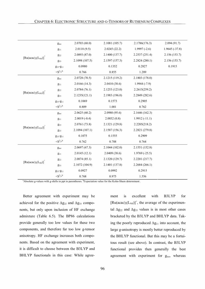
CHAPTER 6: ELECTRONIC STRUCTURE AND G-TENSORS OF RUTHENIUM COMPLEXES
96
giso 2.0703 (68.0) 2.1081 (105.7) 2.1786(176.3) 2.094 (91.7)
g11 2.0118 (9.5) 2.0245 (22.2) 1.9997 (-2.6) 1.9645 (-37.8)
g22 2.0893 (87.0) 2.1400 (137.7) 2.2537 (251.4) 2.156 (153.7)
g33 2.1098 (107.5) 2.1597 (157.3) 2.2824 (280.1) 2.156 (153.7)
g33-g11 0.0980 0.1352 0.2827 0.1915
[Ru(acac)2(LNS)]+
<S2>b 0.766 0.855 1.289
giso 2.0728 (70.5) 2.1215 (119.2) 2.1803 (178.0)
g11 2.0166 (14.3) 2.0410 (38.6) 1.9944 (-7.9)
g22 2.0784 (76.1) 2.1253 (123.0) 2.2615(259.2)
g33 2.1235(121.1) 2.1983 (196.0) 2.2849 (282.6)
g33-g11 0.1069 0.1573 0.2905
[Ru(acac)2(LOO)]+
<S2>b 0.809 1.001 0.762
giso 2.0625 (60.2) 2.0980 (95.6) 2.1646 (162.3)
g11 2.0019 (-0.4) 2.0032 (0.8) 1.9912 (-11.1)
g22 2.0761 (73.8) 2.1321 (129.8) 2.2205(218.2)
g33 2.1094 (107.1) 2.1587 (156.3) 2.2821 (279.8)
g33-g11 0.1075 0.1555 0.2909
[Ru(acac)2(LNN)]+
<S2>b 0.762 0.788 0.764
giso 2.0697 (67.3) 2.1044 (102.0) 2.1551 (152.8)
g11 2.0145 (12.1) 2.0409 (38.6) 1.9769 (-25.5)
g22 2.0874 (85.1) 2.1320 (129.7) 2.2201 (217.7)
g33 2.1072 (104.9) 2.1401 (137.8) 2.2684 (266.1)
g33-g11 0.0927 0.0992 0.2915
[Ru(acac)2(LSS)]+
<S2>b 0.768 0.975 1.556 aAbsolute g-values with g-shifts in ppt in parentheses. bExpectation value for the Kohn-Sham determinant .
Better agreement with experiment may be
achieved for the positive ∆g22 and ∆g33 compo-
nents, but only upon inclusion of HF exchange
admixture (Table 6.5). The BP86 calculations
provide generally too low values for these two
components, and therefore far too low g-tensor
anisotropy. HF exchange increases both compo-
nents. Based on the agreement with experiment,
it is difficult to choose between the B3LYP and
BHLYP functionals in this case: While agree-
ment is excellent with B3LYP for
[Ru(acac)2(LNS)]+, the average of the experimen-
tal ∆g22 and ∆g33 values is in most other cases
bracketed by the B3LYP and BHLYP data. Tak-
ing the poorly reproduced ∆g11 into account, the
large g-anisotropy is mostly better reproduced by
the BHLYP functional. But this may be a fortui-
tous result (see above). In contrast, the B3LYP
functional provides then generally the best
agreement with experiment for giso, whereas
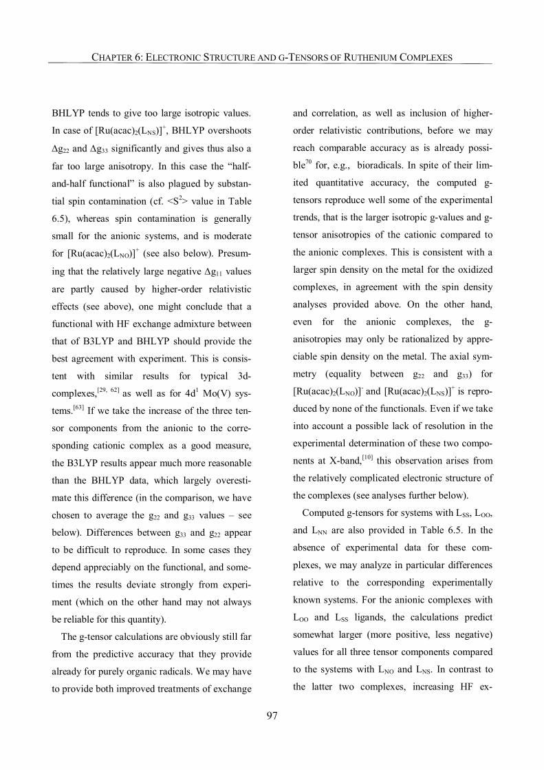
CHAPTER 6: ELECTRONIC STRUCTURE AND G-TENSORS OF RUTHENIUM COMPLEXES
97
BHLYP tends to give too large isotropic values.
In case of [Ru(acac)2(LNS)]+, BHLYP overshoots
∆g22 and ∆g33 significantly and gives thus also a
far too large anisotropy. In this case the “half-
and-half functional” is also plagued by substan-
tial spin contamination (cf. <S2> value in Table
6.5), whereas spin contamination is generally
small for the anionic systems, and is moderate
for [Ru(acac)2(LNO)]+ (see also below). Presum-
ing that the relatively large negative ∆g11 values
are partly caused by higher-order relativistic
effects (see above), one might conclude that a
functional with HF exchange admixture between
that of B3LYP and BHLYP should provide the
best agreement with experiment. This is consis-
tent with similar results for typical 3d-
complexes,[29, 62] as well as for 4d1 Mo(V) sys-
tems.[63] If we take the increase of the three ten-
sor components from the anionic to the corre-
sponding cationic complex as a good measure,
the B3LYP results appear much more reasonable
than the BHLYP data, which largely overesti-
mate this difference (in the comparison, we have
chosen to average the g22 and g33 values – see
below). Differences between g33 and g22 appear
to be difficult to reproduce. In some cases they
depend appreciably on the functional, and some-
times the results deviate strongly from experi-
ment (which on the other hand may not always
be reliable for this quantity).
The g-tensor calculations are obviously still far
from the predictive accuracy that they provide
already for purely organic radicals. We may have
to provide both improved treatments of exchange
and correlation, as well as inclusion of higher-
order relativistic contributions, before we may
reach comparable accuracy as is already possi-
ble70 for, e.g., bioradicals. In spite of their lim-
ited quantitative accuracy, the computed g-
tensors reproduce well some of the experimental
trends, that is the larger isotropic g-values and g-
tensor anisotropies of the cationic compared to
the anionic complexes. This is consistent with a
larger spin density on the metal for the oxidized
complexes, in agreement with the spin density
analyses provided above. On the other hand,
even for the anionic complexes, the g-
anisotropies may only be rationalized by appre-
ciable spin density on the metal. The axial sym-
metry (equality between g22 and g33) for
[Ru(acac)2(LNO)]- and [Ru(acac)2(LNS)]+ is repro-
duced by none of the functionals. Even if we take
into account a possible lack of resolution in the
experimental determination of these two compo-
nents at X-band,[10] this observation arises from
the relatively complicated electronic structure of
the complexes (see analyses further below).
Computed g-tensors for systems with LSS, LOO,
and LNN are also provided in Table 6.5. In the
absence of experimental data for these com-
plexes, we may analyze in particular differences
relative to the corresponding experimentally
known systems. For the anionic complexes with
LOO and LSS ligands, the calculations predict
somewhat larger (more positive, less negative)
values for all three tensor components compared
to the systems with LNO and LNS. In contrast to
the latter two complexes, increasing HF ex-
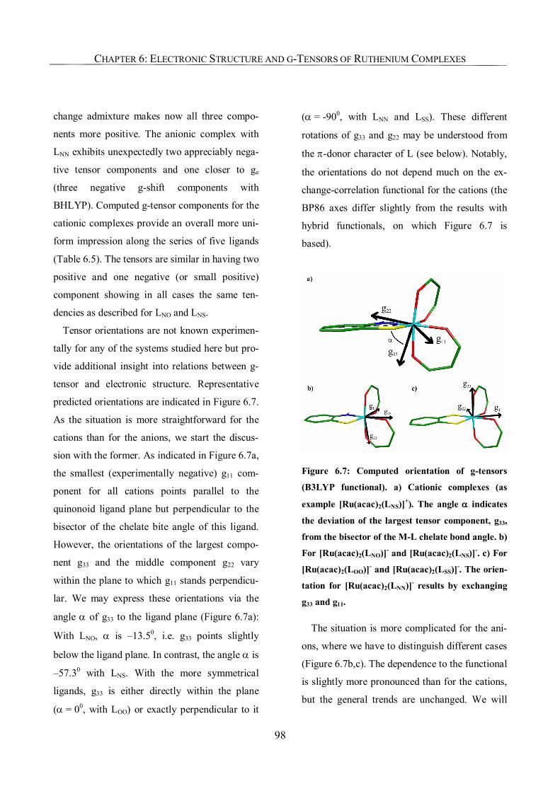
CHAPTER 6: ELECTRONIC STRUCTURE AND G-TENSORS OF RUTHENIUM COMPLEXES
98
change admixture makes now all three compo-
nents more positive. The anionic complex with
LNN exhibits unexpectedly two appreciably nega-
tive tensor components and one closer to ge
(three negative g-shift components with
BHLYP). Computed g-tensor components for the
cationic complexes provide an overall more uni-
form impression along the series of five ligands
(Table 6.5). The tensors are similar in having two
positive and one negative (or small positive)
component showing in all cases the same ten-
dencies as described for LNO and LNS.
Tensor orientations are not known experimen-
tally for any of the systems studied here but pro-
vide additional insight into relations between g-
tensor and electronic structure. Representative
predicted orientations are indicated in Figure 6.7.
As the situation is more straightforward for the
cations than for the anions, we start the discus-
sion with the former. As indicated in Figure 6.7a,
the smallest (experimentally negative) g11 com-
ponent for all cations points parallel to the
quinonoid ligand plane but perpendicular to the
bisector of the chelate bite angle of this ligand.
However, the orientations of the largest compo-
nent g33 and the middle component g22 vary
within the plane to which g11 stands perpendicu-
lar. We may express these orientations via the
angle α of g33 to the ligand plane (Figure 6.7a):
With LNO, α is –13.50, i.e. g33 points slightly
below the ligand plane. In contrast, the angle α is
–57.30 with LNS. With the more symmetrical
ligands, g33 is either directly within the plane
(α = 00, with LOO) or exactly perpendicular to it
(α = -900, with LNN and LSS). These different
rotations of g33 and g22 may be understood from
the π-donor character of L (see below). Notably,
the orientations do not depend much on the ex-
change-correlation functional for the cations (the
BP86 axes differ slightly from the results with
hybrid functionals, on which Figure 6.7 is
based).
Figure 6.7: Computed orientation of g-tensors
(B3LYP functional). a) Cationic complexes (as
example [Ru(acac)2(LNS)]+). The angle α indicates
the deviation of the largest tensor component, g33,
from the bisector of the M-L chelate bond angle. b)
For [Ru(acac)2(LNO)]- and [Ru(acac)2(LNS)]-. c) For
[Ru(acac)2(LOO)]- and [Ru(acac)2(LSS)]-. The orien-
tation for [Ru(acac)2(LNN)]- results by exchanging
g33 and g11.
The situation is more complicated for the ani-
ons, where we have to distinguish different cases
(Figure 6.7b,c). The dependence to the functional
is slightly more pronounced than for the cations,
but the general trends are unchanged. We will
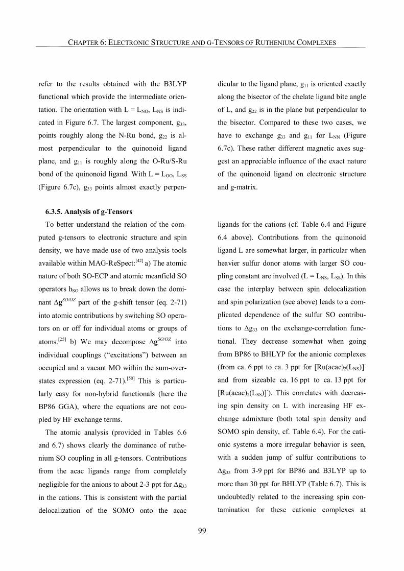
CHAPTER 6: ELECTRONIC STRUCTURE AND G-TENSORS OF RUTHENIUM COMPLEXES
99
refer to the results obtained with the B3LYP
functional which provide the intermediate orien-
tation. The orientation with L = LNO, LNS is indi-
cated in Figure 6.7. The largest component, g33,
points roughly along the N-Ru bond, g22 is al-
most perpendicular to the quinonoid ligand
plane, and g11 is roughly along the O-Ru/S-Ru
bond of the quinonoid ligand. With L = LOO, LSS
(Figure 6.7c), g33 points almost exactly perpen-
dicular to the ligand plane, g11 is oriented exactly
along the bisector of the chelate ligand bite angle
of L, and g22 is in the plane but perpendicular to
the bisector. Compared to these two cases, we
have to exchange g33 and g11 for LNN (Figure
6.7c). These rather different magnetic axes sug-
gest an appreciable influence of the exact nature
of the quinonoid ligand on electronic structure
and g-matrix.
6.3.5. Analysis of g-Tensors
To better understand the relation of the com-
puted g-tensors to electronic structure and spin
density, we have made use of two analysis tools
available within MAG-ReSpect:[42] a) The atomic
nature of both SO-ECP and atomic meanfield SO
operators hSO allows us to break down the domi-
nant ∆gSO/OZ part of the g-shift tensor (eq. 2-71)
into atomic contributions by switching SO opera-
tors on or off for individual atoms or groups of
atoms.[25] b) We may decompose ∆gSO/OZ into
individual couplings (“excitations”) between an
occupied and a vacant MO within the sum-over-
states expression (eq. 2-71).[50] This is particu-
larly easy for non-hybrid functionals (here the
BP86 GGA), where the equations are not cou-
pled by HF exchange terms.
The atomic analysis (provided in Tables 6.6
and 6.7) shows clearly the dominance of ruthe-
nium SO coupling in all g-tensors. Contributions
from the acac ligands range from completely
negligible for the anions to about 2-3 ppt for ∆g33
in the cations. This is consistent with the partial
delocalization of the SOMO onto the acac
ligands for the cations (cf. Table 6.4 and Figure
6.4 above). Contributions from the quinonoid
ligand L are somewhat larger, in particular when
heavier sulfur donor atoms with larger SO cou-
pling constant are involved (L = LNS, LSS). In this
case the interplay between spin delocalization
and spin polarization (see above) leads to a com-
plicated dependence of the sulfur SO contribu-
tions to ∆g33 on the exchange-correlation func-
tional. They decrease somewhat when going
from BP86 to BHLYP for the anionic complexes
(from ca. 6 ppt to ca. 3 ppt for [Ru(acac)2(LNS)]-
and from sizeable ca. 16 ppt to ca. 13 ppt for
[Ru(acac)2(LSS)]-). This correlates with decreas-
ing spin density on L with increasing HF ex-
change admixture (both total spin density and
SOMO spin density, cf. Table 6.4). For the cati-
onic systems a more irregular behavior is seen,
with a sudden jump of sulfur contributions to
∆g33 from 3-9 ppt for BP86 and B3LYP up to
more than 30 ppt for BHLYP (Table 6.7). This is
undoubtedly related to the increasing spin con-
tamination for these cationic complexes at
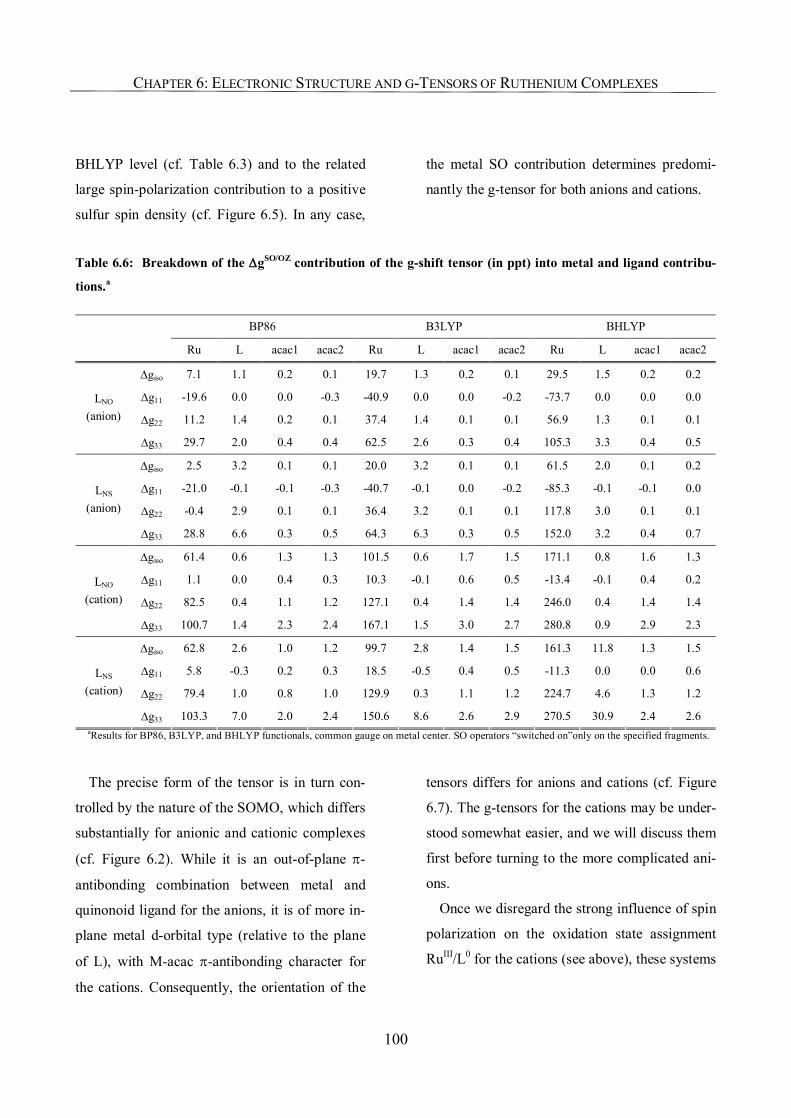
CHAPTER 6: ELECTRONIC STRUCTURE AND G-TENSORS OF RUTHENIUM COMPLEXES
100
BHLYP level (cf. Table 6.3) and to the related
large spin-polarization contribution to a positive
sulfur spin density (cf. Figure 6.5). In any case,
the metal SO contribution determines predomi-
nantly the g-tensor for both anions and cations.
Table 6.6: Breakdown of the ∆gSO/OZ contribution of the g-shift tensor (in ppt) into metal and ligand contribu-
tions.a
BP86 B3LYP BHLYP
Ru L acac1 acac2 Ru L acac1 acac2 Ru L acac1 acac2
∆giso 7.1 1.1 0.2 0.1 19.7 1.3 0.2 0.1 29.5 1.5 0.2 0.2
∆g11 -19.6 0.0 0.0 -0.3 -40.9 0.0 0.0 -0.2 -73.7 0.0 0.0 0.0
∆g22 11.2 1.4 0.2 0.1 37.4 1.4 0.1 0.1 56.9 1.3 0.1 0.1
LNO (anion)
∆g33 29.7 2.0 0.4 0.4 62.5 2.6 0.3 0.4 105.3 3.3 0.4 0.5
∆giso 2.5 3.2 0.1 0.1 20.0 3.2 0.1 0.1 61.5 2.0 0.1 0.2
∆g11 -21.0 -0.1 -0.1 -0.3 -40.7 -0.1 0.0 -0.2 -85.3 -0.1 -0.1 0.0
∆g22 -0.4 2.9 0.1 0.1 36.4 3.2 0.1 0.1 117.8 3.0 0.1 0.1
LNS (anion)
∆g33 28.8 6.6 0.3 0.5 64.3 6.3 0.3 0.5 152.0 3.2 0.4 0.7
∆giso 61.4 0.6 1.3 1.3 101.5 0.6 1.7 1.5 171.1 0.8 1.6 1.3
∆g11 1.1 0.0 0.4 0.3 10.3 -0.1 0.6 0.5 -13.4 -0.1 0.4 0.2
∆g22 82.5 0.4 1.1 1.2 127.1 0.4 1.4 1.4 246.0 0.4 1.4 1.4
LNO (cation)
∆g33 100.7 1.4 2.3 2.4 167.1 1.5 3.0 2.7 280.8 0.9 2.9 2.3
∆giso 62.8 2.6 1.0 1.2 99.7 2.8 1.4 1.5 161.3 11.8 1.3 1.5
∆g11 5.8 -0.3 0.2 0.3 18.5 -0.5 0.4 0.5 -11.3 0.0 0.0 0.6
∆g22 79.4 1.0 0.8 1.0 129.9 0.3 1.1 1.2 224.7 4.6 1.3 1.2
LNS (cation)
∆g33 103.3 7.0 2.0 2.4 150.6 8.6 2.6 2.9 270.5 30.9 2.4 2.6 aResults for BP86, B3LYP, and BHLYP functionals, common gauge on metal center. SO operators “switched on”only on the specified fragments.
The precise form of the tensor is in turn con-
trolled by the nature of the SOMO, which differs
substantially for anionic and cationic complexes
(cf. Figure 6.2). While it is an out-of-plane π-
antibonding combination between metal and
quinonoid ligand for the anions, it is of more in-
plane metal d-orbital type (relative to the plane
of L), with M-acac π-antibonding character for
the cations. Consequently, the orientation of the
tensors differs for anions and cations (cf. Figure
6.7). The g-tensors for the cations may be under-
stood somewhat easier, and we will discuss them
first before turning to the more complicated ani-
ons.
Once we disregard the strong influence of spin
polarization on the oxidation state assignment
RuIII/L0 for the cations (see above), these systems
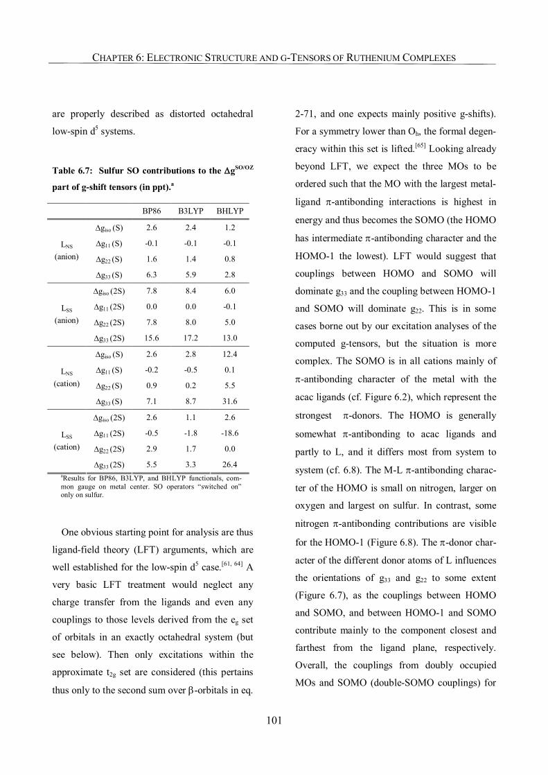
CHAPTER 6: ELECTRONIC STRUCTURE AND G-TENSORS OF RUTHENIUM COMPLEXES
101
are properly described as distorted octahedral
low-spin d5 systems.
Table 6.7: Sulfur SO contributions to the ∆gSO/OZ
part of g-shift tensors (in ppt).a
BP86 B3LYP BHLYP
∆giso (S) 2.6 2.4 1.2
∆g11 (S) -0.1 -0.1 -0.1
∆g22 (S) 1.6 1.4 0.8
LNS (anion)
∆g33 (S) 6.3 5.9 2.8
∆giso (2S) 7.8 8.4 6.0
∆g11 (2S) 0.0 0.0 -0.1
∆g22 (2S) 7.8 8.0 5.0
LSS (anion)
∆g33 (2S) 15.6 17.2 13.0
∆giso (S) 2.6 2.8 12.4
∆g11 (S) -0.2 -0.5 0.1
∆g22 (S) 0.9 0.2 5.5
LNS (cation)
∆g33 (S) 7.1 8.7 31.6
∆giso (2S) 2.6 1.1 2.6
∆g11 (2S) -0.5 -1.8 -18.6
∆g22 (2S) 2.9 1.7 0.0
LSS (cation)
∆g33 (2S) 5.5 3.3 26.4 aResults for BP86, B3LYP, and BHLYP functionals, com-mon gauge on metal center. SO operators “switched on” only on sulfur.
One obvious starting point for analysis are thus
ligand-field theory (LFT) arguments, which are
well established for the low-spin d5 case.[61, 64] A
very basic LFT treatment would neglect any
charge transfer from the ligands and even any
couplings to those levels derived from the eg set
of orbitals in an exactly octahedral system (but
see below). Then only excitations within the
approximate t2g set are considered (this pertains
thus only to the second sum over β-orbitals in eq.
2-71, and one expects mainly positive g-shifts).
For a symmetry lower than Oh, the formal degen-
eracy within this set is lifted.[65] Looking already
beyond LFT, we expect the three MOs to be
ordered such that the MO with the largest metal-
ligand π-antibonding interactions is highest in
energy and thus becomes the SOMO (the HOMO
has intermediate π-antibonding character and the
HOMO-1 the lowest). LFT would suggest that
couplings between HOMO and SOMO will
dominate g33 and the coupling between HOMO-1
and SOMO will dominate g22. This is in some
cases borne out by our excitation analyses of the
computed g-tensors, but the situation is more
complex. The SOMO is in all cations mainly of
π-antibonding character of the metal with the
acac ligands (cf. Figure 6.2), which represent the
strongest π-donors. The HOMO is generally
somewhat π-antibonding to acac ligands and
partly to L, and it differs most from system to
system (cf. 6.8). The M-L π-antibonding charac-
ter of the HOMO is small on nitrogen, larger on
oxygen and largest on sulfur. In contrast, some
nitrogen π-antibonding contributions are visible
for the HOMO-1 (Figure 6.8). The π-donor char-
acter of the different donor atoms of L influences
the orientations of g33 and g22 to some extent
(Figure 6.7), as the couplings between HOMO
and SOMO, and between HOMO-1 and SOMO
contribute mainly to the component closest and
farthest from the ligand plane, respectively.
Overall, the couplings from doubly occupied
MOs and SOMO (double-SOMO couplings) for
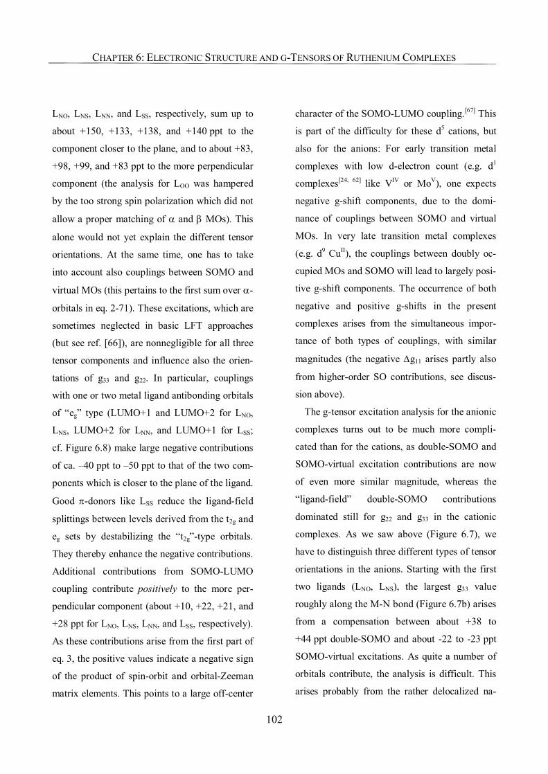
CHAPTER 6: ELECTRONIC STRUCTURE AND G-TENSORS OF RUTHENIUM COMPLEXES
102
LNO, LNS, LNN, and LSS, respectively, sum up to
about +150, +133, +138, and +140 ppt to the
component closer to the plane, and to about +83,
+98, +99, and +83 ppt to the more perpendicular
component (the analysis for LOO was hampered
by the too strong spin polarization which did not
allow a proper matching of α and β MOs). This
alone would not yet explain the different tensor
orientations. At the same time, one has to take
into account also couplings between SOMO and
virtual MOs (this pertains to the first sum over α-
orbitals in eq. 2-71). These excitations, which are
sometimes neglected in basic LFT approaches
(but see ref. [66]), are nonnegligible for all three
tensor components and influence also the orien-
tations of g33 and g22. In particular, couplings
with one or two metal ligand antibonding orbitals
of “eg” type (LUMO+1 and LUMO+2 for LNO,
LNS, LUMO+2 for LNN, and LUMO+1 for LSS;
cf. Figure 6.8) make large negative contributions
of ca. –40 ppt to –50 ppt to that of the two com-
ponents which is closer to the plane of the ligand.
Good π-donors like LSS reduce the ligand-field
splittings between levels derived from the t2g and
eg sets by destabilizing the “t2g”-type orbitals.
They thereby enhance the negative contributions.
Additional contributions from SOMO-LUMO
coupling contribute positively to the more per-
pendicular component (about +10, +22, +21, and
+28 ppt for LNO, LNS, LNN, and LSS, respectively).
As these contributions arise from the first part of
eq. 3, the positive values indicate a negative sign
of the product of spin-orbit and orbital-Zeeman
matrix elements. This points to a large off-center
character of the SOMO-LUMO coupling.[67] This
is part of the difficulty for these d5 cations, but
also for the anions: For early transition metal
complexes with low d-electron count (e.g. d1
complexes[24, 62] like VIV or MoV), one expects
negative g-shift components, due to the domi-
nance of couplings between SOMO and virtual
MOs. In very late transition metal complexes
(e.g. d9 CuII), the couplings between doubly oc-
cupied MOs and SOMO will lead to largely posi-
tive g-shift components. The occurrence of both
negative and positive g-shifts in the present
complexes arises from the simultaneous impor-
tance of both types of couplings, with similar
magnitudes (the negative ∆g11 arises partly also
from higher-order SO contributions, see discus-
sion above).
The g-tensor excitation analysis for the anionic
complexes turns out to be much more compli-
cated than for the cations, as double-SOMO and
SOMO-virtual excitation contributions are now
of even more similar magnitude, whereas the
“ligand-field” double-SOMO contributions
dominated still for g22 and g33 in the cationic
complexes. As we saw above (Figure 6.7), we
have to distinguish three different types of tensor
orientations in the anions. Starting with the first
two ligands (LNO, LNS), the largest g33 value
roughly along the M-N bond (Figure 6.7b) arises
from a compensation between about +38 to
+44 ppt double-SOMO and about -22 to -23 ppt
SOMO-virtual excitations. As quite a number of
orbitals contribute, the analysis is difficult. This
arises probably from the rather delocalized na-
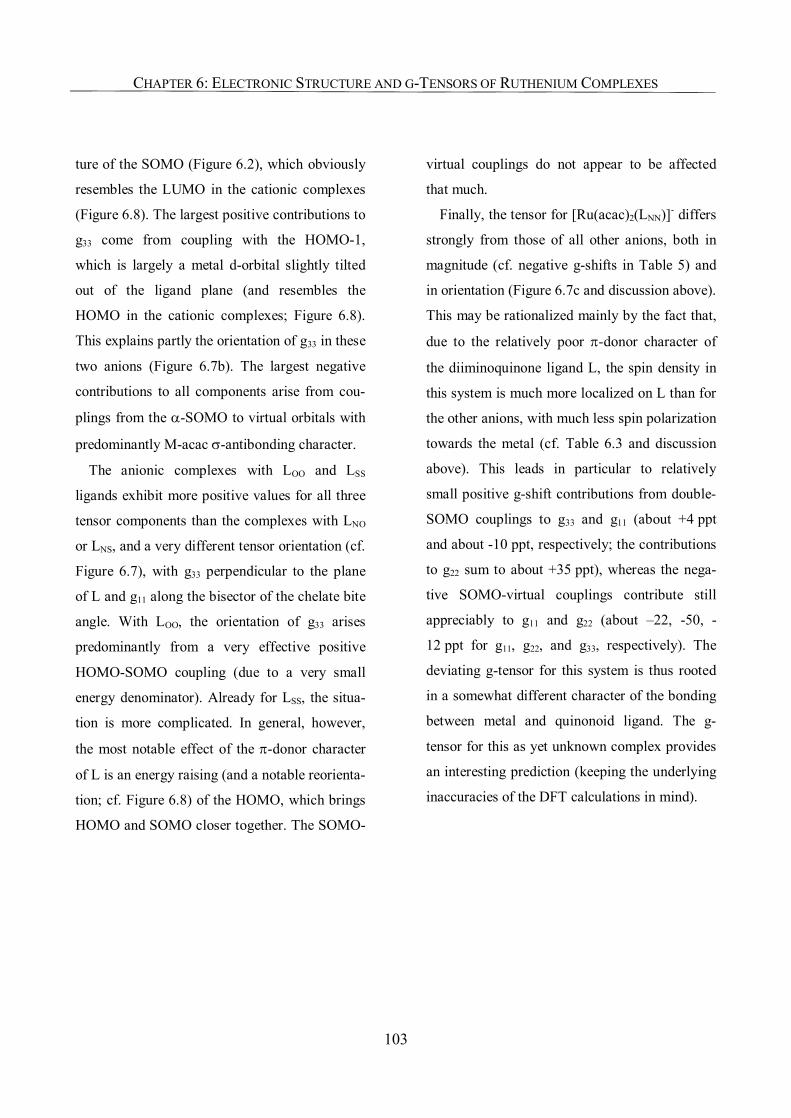
CHAPTER 6: ELECTRONIC STRUCTURE AND G-TENSORS OF RUTHENIUM COMPLEXES
103
ture of the SOMO (Figure 6.2), which obviously
resembles the LUMO in the cationic complexes
(Figure 6.8). The largest positive contributions to
g33 come from coupling with the HOMO-1,
which is largely a metal d-orbital slightly tilted
out of the ligand plane (and resembles the
HOMO in the cationic complexes; Figure 6.8).
This explains partly the orientation of g33 in these
two anions (Figure 6.7b). The largest negative
contributions to all components arise from cou-
plings from the α-SOMO to virtual orbitals with
predominantly M-acac σ-antibonding character.
The anionic complexes with LOO and LSS
ligands exhibit more positive values for all three
tensor components than the complexes with LNO
or LNS, and a very different tensor orientation (cf.
Figure 6.7), with g33 perpendicular to the plane
of L and g11 along the bisector of the chelate bite
angle. With LOO, the orientation of g33 arises
predominantly from a very effective positive
HOMO-SOMO coupling (due to a very small
energy denominator). Already for LSS, the situa-
tion is more complicated. In general, however,
the most notable effect of the π-donor character
of L is an energy raising (and a notable reorienta-
tion; cf. Figure 6.8) of the HOMO, which brings
HOMO and SOMO closer together. The SOMO-
virtual couplings do not appear to be affected
that much.
Finally, the tensor for [Ru(acac)2(LNN)]- differs
strongly from those of all other anions, both in
magnitude (cf. negative g-shifts in Table 5) and
in orientation (Figure 6.7c and discussion above).
This may be rationalized mainly by the fact that,
due to the relatively poor π-donor character of
the diiminoquinone ligand L, the spin density in
this system is much more localized on L than for
the other anions, with much less spin polarization
towards the metal (cf. Table 6.3 and discussion
above). This leads in particular to relatively
small positive g-shift contributions from double-
SOMO couplings to g33 and g11 (about +4 ppt
and about -10 ppt, respectively; the contributions
to g22 sum to about +35 ppt), whereas the nega-
tive SOMO-virtual couplings contribute still
appreciably to g11 and g22 (about –22, -50, -
12 ppt for g11, g22, and g33, respectively). The
deviating g-tensor for this system is thus rooted
in a somewhat different character of the bonding
between metal and quinonoid ligand. The g-
tensor for this as yet unknown complex provides
an interesting prediction (keeping the underlying
inaccuracies of the DFT calculations in mind).
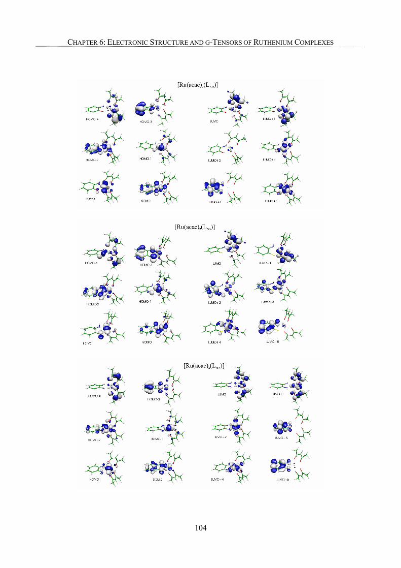
CHAPTER 6: ELECTRONIC STRUCTURE AND G-TENSORS OF RUTHENIUM COMPLEXES
104
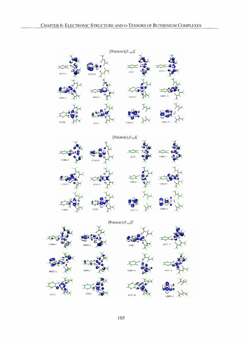
CHAPTER 6: ELECTRONIC STRUCTURE AND G-TENSORS OF RUTHENIUM COMPLEXES
105
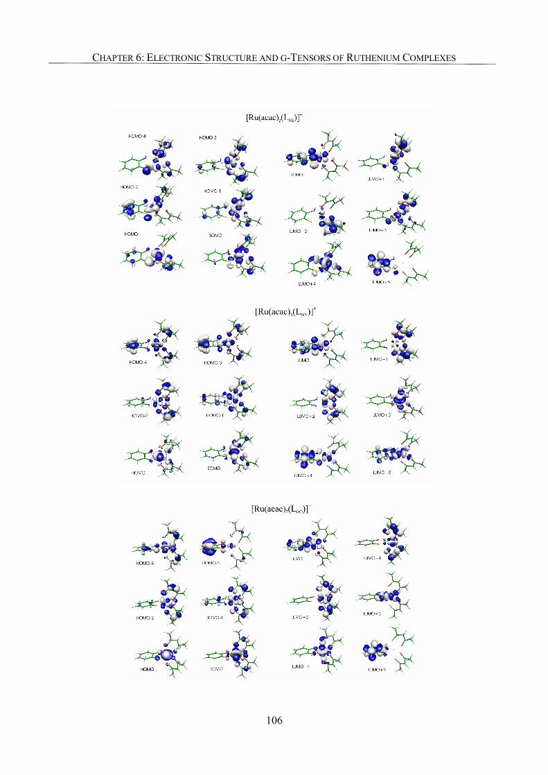
CHAPTER 6: ELECTRONIC STRUCTURE AND G-TENSORS OF RUTHENIUM COMPLEXES
106
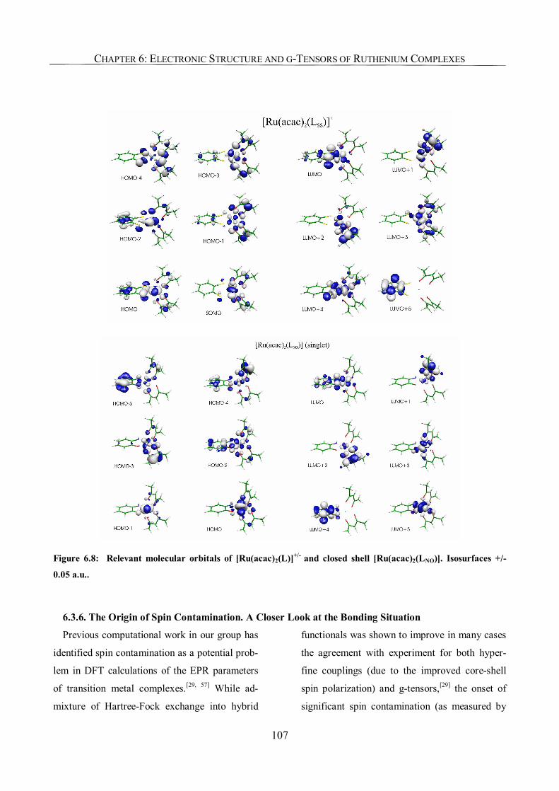
CHAPTER 6: ELECTRONIC STRUCTURE AND G-TENSORS OF RUTHENIUM COMPLEXES
107
Figure 6.8: Relevant molecular orbitals of [Ru(acac)2(L)]+/- and closed shell [Ru(acac)2(LNO)]. Isosurfaces +/-
0.05 a.u..
6.3.6. The Origin of Spin Contamination. A Closer Look at the Bonding Situation
Previous computational work in our group has
identified spin contamination as a potential prob-
lem in DFT calculations of the EPR parameters
of transition metal complexes.[29, 57] While ad-
mixture of Hartree-Fock exchange into hybrid
functionals was shown to improve in many cases
the agreement with experiment for both hyper-
fine couplings (due to the improved core-shell
spin polarization) and g-tensors,[29] the onset of
significant spin contamination (as measured by
CHAPTER 6: ELECTRONIC STRUCTURE AND G-TENSORS OF RUTHENIUM COMPLEXES
108
the S2 expectation value of the KS determinant)
with increasing HF exchange tended to deterio-
rate both properties (including the otherwise not
very sensitive dipolar metal hyperfine cou-
plings[57]) for some systems. Closer analysis in-
dicated[68] that spin contamination in typical
complexes with predominantly metal-centered
spin density arises in particular when the SOMO
exhibits appreciable metal-ligand antibonding
character. The spin contamination was found to
be related to appreciable spin polarization of
doubly occupied valence orbitals, mainly of
metal-ligand bonding character,[68] coupled to the
admixture of low-lying excited states of higher
spin multiplicity.
The observed increase of spin contamination
with increasing HF exchange[29, 57] becomes then
understandable, as unrestricted Hartree-Fock
wavefunctions tend to appreciably overestimate
spin polarization. A larger fraction of HF ex-
change will thus make the wavefunction more
unstable with respect to admixture of high-spin
contaminants. Therefore, the trends in the <S2>
expectation values of several of the cationic
complexes in Table 5 were very unexpected (the
anionic complexes show very small spin con-
tamination and no unusual trends): While the
complexes with sulfur donor atoms in the
quinonoid ligand (i.e. with LNS and LSS) exhibit
the expected increase of spin contamination
along the series BP86 < B3LYP < BHLYP, all
other cationic complexes have the largest values
for the B3LYP functional, and a lower value for
BHLYP. Except for one case (LNN, but note the
small difference of only 0.02), the BHLYP <S2>
value is even below the BP86 value (Table 6.5)!
To our knowledge, behavior like this has not
been observed before, and it is worth a closer
analysis. We recall that the predominantly metal-
centered spin density in the cationic complexes
arises primarily from spin-polarization contribu-
tions (cf. Table 6.3 and Figure 6.4). However,
this alone does not explain the different depend-
ence of <S2> on HF exchange admixture for,
e.g., [Ru(acac)2(LNO)]+ and [Ru(acac)2(LNS)]+. In
both cases, the SOMO has appreciable spin den-
sity on the acac ligands, which is largely com-
pensated by the negative spin-polarization con-
tributions (Figure 6.5). Notably, however, for the
sulfur-containing complex increasing admixture
of HF exchange builds up strong negative spin
density, caused by spin polarization, on certain
atoms within the quinonoid ligand. In contrast,
for [Ru(acac)2(LNO)]+ this negative spin density
is already less pronounced at B3LYP level and
vanishes essentially with BHLYP. As a result,
appreciable negative total spin density remains
on N, C2, C4, and C6, in [Ru(acac)2(LNS)]+ but
not in [Ru(acac)2(LNO)]+ (Figure 4). Figure 6.7
deconstructs the spin-polarization part of the
total spin density of [Ru(acac)2(LNO)]+ into the
major contributions from individual doubly oc-
cupied MOs, both for B3LYP and for BHLYP
functionals. Negative spin polarization on oxy-
gen in L arises mainly from the HOMO for
B3LYP, and this contribution vanishes for
BHLYP.
CHAPTER 6: ELECTRONIC STRUCTURE AND G-TENSORS OF RUTHENIUM COMPLEXES
109
Obviously, the presence of spin polarization
alone does not explain the strange trends of spin
contamination for some of the cationic com-
plexes (even the anionic complexes exhibit
strong spin polarization; Figure 6.3, Table 6.4).
The observed differences in the accumulation of
negative spin density on some atoms in the
quinonoid ligand is, however, at the heart of the
different spin contamination. Examination of
unrestricted natural orbitals (NOs; Figure 6.9)
allows a deeper rationalization. In the absence of
spin contamination one would expect for these
complexes only one singly occupied NO together
with exactly doubly occupied or exactly empty
NOs.[69] Spin contamination will appear as a
depletion of some formally doubly occupied NOs
and concomitant partial occupation of formally
empty NOs. Fortunately, in the title systems this
pertains only to maximally one pair of a formally
occupied and a formally empty NO (termed λ
and µ, respectively, in Figure 6.9). The singly
occupied NO is termed a2. It resembles the ca-
nonical SOMO (Figure 6.2), but with somewhat
less delocalization onto the acac ligands.
Most interestingly, the deviation of λ and µ
NOs from integer occupation in
[Ru(acac)2(LNO)]+ is notable for B3LYP but be-
low the chosen threshold of 0.01 a.u. for BHLYP
(Figure 6.9). In contrast, in [Ru(acac)2(LNS)]+ the
NOs deviate from integer occupation for both
functionals. Closer inspection indicates notable
differences between the character of these NOs
for the two complexes. In [Ru(acac)2(LNO)]+, the
λ NO is largely nonbonding between the metal
and the quinonoid ligand, whereas the µ NO is
moderately metal-ligand antibonding (less so for
BHLYP than for B3LYP). The presence of sulfur
in [Ru(acac)2(LNS)]+ alters the situation. Now the
λ-NO is already appreciably Ru-N bonding at
B3LYP level and becomes even more strongly
Ru-S bonding with BHLYP. The µ-NO is gener-
ally more appreciably antibonding than in the
absence of sulfur (Figure 6.9). In agreement with
previous analyses,[68] the enhanced spin contami-
nation with increasing HF exchange admixture
for [Ru(acac)2(LNS)]+ is thus related to spin po-
larization across a relatively covalent metal-
ligand bond. In contrast, in [Ru(acac)2(LNO)]+ the
increased HF exchange admixture leads essen-
tially to a demixing of λ and µ NOs (less interac-
tions between metal and ligand), due to the in-
creased bond ionicity. We conclude thus that the
unusual trend in the <S2> values for the cationic
complexes without sulfur ligands are due to an
interplay between two opposing trends: Increas-
ing HF exchange admixture renders the metal-
ligand bond more ionic, and at the same time it
increases general spin polarization. While the
latter effect tends to increase <S2>, the former
counteracts this trend by diminishing the in-
volvement of the metal-ligand bond in the spin
polarization process. Covalency is more pro-
nounced in the presence of sulfur, and increased
spin polarization pervails over a reduction of
covalency.
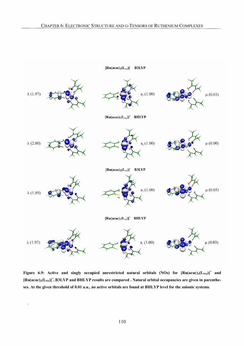
CHAPTER 6: ELECTRONIC STRUCTURE AND G-TENSORS OF RUTHENIUM COMPLEXES
110
Figure 6.9: Active and singly occupied unrestricted natural orbitals (NOs) for [Ru(acac)2(LNO)]+ and
[Ru(acac)2(LNS)]+. B3LYP and BHLYP results are compared . Natural orbital occupancies are given in parenthe-
ses. At the given threshold of 0.01 a.u., no active orbitals are found at BHLYP level for the anionic systems.
´
CHAPTER 6: ELECTRONIC STRUCTURE AND G-TENSORS OF RUTHENIUM COMPLEXES
111
6.4. Conclusions
The determination of the actual redox state of
metal and ligand(s) in biological redox processes
is often far from trivial (the ligand spin and
charge state may sometimes even depend on the
protein environment[70]). Here we have shown for
a series of ruthenium complexes with biologi-
cally relevant o-quinone-type ligands, that the
formal redox state of metal and ligand may be
bracketed in remarkable detail by state-of-the-art
quantum chemical tools. Indeed, the careful
combination of spin density, charge density, and
different molecular-orbital analyses, together
with studies of molecular structure and electronic
g-tensors, provided a much more refined view of
redox states than previous analyses of experi-
mental structures and EPR spectra alone.
In particular, the singlet closed-shell ground
state of the neutral title complexes
[Ru(acac)2(L)] (L = o-quinonoid ligand) turns
out to be better described by a superposition of
RuIII/L- and RuII/L0 states rather than by a pure
RuIII/L- formulation. The anionic complexes are
best described as intermediate between RuIII/L2-
and RuII/L-. In contrast, the triplet excited state of
the neutral complexes comes close to a pure
RuIII/L- description, and the cationic complexes
appear best described by an assignment RuIII/L0.
In view of the computed structure parameters for
various systems, these findings require some
modification of previously proposed interrela-
tions between intraligand bond lengths and pos-
sible integer “physical” redox states of metal and
ligand.[51] Often, the true situation in a given
complex may be intermediate between integer
oxidation numbers, and the structural data are
expected to reflect this.
A somewhat surprising finding of this study is
the appreciable importance of spin polarization
in the unrestricted Kohn-Sham description of
electronic structure and formal redox states for
the open-shell systems. This holds both for the
anionic and for the cationic complexes, as well
as for the triplet excited state of the neutral com-
plexes. While the metal-ligand antibonding SO-
MOs were delocalized to an unrealistically large
extent onto the ligands (mainly onto L for the
anions and onto acac for the cations), spin po-
larization of doubly occupied MOs with more or
less metal-ligand bonding character remedied the
situation and provided a rather different final
charge- and spin-density distribution (with the
interesting exception of the as yet unknown ani-
onic complex [Ru(acac)2(LNN)]-). It is likely that
this will be a common situation also for DFT
calculations on other open-shell transition metal
complexes with redox-active ligands. While spin
polarization is well known to be important for
the interpretation of electronic structure and spin
coupling in multinuclear complexes,[64] we are
not aware of any previous study that demon-
strated a fundamental importance of spin polari-
zation for the assignment of oxidation state in a
mononuclear complex.
We noticed also an unusual behavior of the
spin contamination of the Kohn-Sham determi-
nant as a function of exchange-correlation func-
CHAPTER 6: ELECTRONIC STRUCTURE AND G-TENSORS OF RUTHENIUM COMPLEXES
112
tional for some but not for all of the cationic
complexes. Closer analysis, in particular of unre-
stricted natural orbitals, revealed partly counter-
acting influences from spin polarization and
metal-ligand covalency.
The relation of electronic g-tensors to elec-
tronic structure and spin-density distribution in
these non-trivial systems was analyzed by means
of MO and atomic spin-orbit analyses in second-
order perturbation theory. Starting from a ligand-
field theory point of view for the formally low-
spin d5-type cationic complexes, we found that a
more refined analysis that includes also SOMO-
virtual excitations is necessary to understand in
particular the orientation of the g33 and g22 tensor
components. The very different and still more
complicated situation for the anionic complexes
arises from a similar magnitude of contributions
from SOMO to virtual space and from doubly-
occupied space to SOMO. The orientation of the
g-tensor in these anionic systems may already be
altered fundamentally by a small modification of
the quinonoid ligand. Beyond some basic fea-
tures discussed in the introduction, and except
for simple, clear-cut cases, it appears difficult at
present to unambiguously assign oxidation states
for open-shell complexes with redox-active
ligands based on the g-tensors alone. Further
quantum chemical analyses, like the ones pre-
sented in this work, appear to be necessary to
reach a new level of classification.
113
Chapter 7
EPR Parameters and Spin-Density Distributions
of Dicopper(I) Complexes with bridging Azo and
Tetrazine Radical Anion Ligands[1]
7.1. Introduction
As mentioned in Chapter 6, the interest in tran-
sition metal complexes with redox-active radical-
anion ligands is fuelled on one side by their role
as models for certain metallo-enzymes such as
galactose oxidase or related systems, and on the
other side by their potential as building blocks in
supermolecular architectures with interesting
electron-transfer and magnetic properties.[1] In
the case of a radical anion bridging two metals, a
main challenge is also to establish reasonable
physical oxidation states for metals and ligand
together with a reliable spin-density distribution.
Recent work on systems with redox-active
ligands has focused on a series of dirhenium
complexes with bridging azo ligands,[3] where
the authors tried to analyze by DFT calculations
data obtained by high-field EPR (see also our
work on Ru complexes with ortho-quinonoid
ligands in Chapter 6). Due to the importance of
higher-order spin-orbit effects and a large de-
pendence of the results on exchange-correlation
functional, the computation of electronic g-
tensors for such systems turned out to be particu-
larly challenging. Hyperfine data were not avail-
able for comparison. To establish the accuracy of
DFT methods for both hyperfine and g-tensors of
such radical-anion dinuclear complexes in a
more meaningful and complete way, and to pro-
vide a basis for qualitative models, we extend the
quantum chemical analyses now to a series of
monocationic dicopper complexes (µ-L)[Cu-
(PR3)2]2+. The dichelating tetradentate ligand L
contains an azo or tetrazine moiety (Scheme 7.1),
and the spin density is thought to be concentrated
mostly on L.
These interesting systems (with PPh3 or
Ph2P(CH2)6PPh2 coligands L) have recently been
studied in detail experimentally by Kaim and
coworkers.[4-7] The advantages of this choice of
target systems for deeper theoretical study are
threefold: (a) for the 3d metal copper, the g-
tensor is expected to be described better by a
perturbational treatment of spin-orbit coupling
than for the abovementioned dirhenium systems.
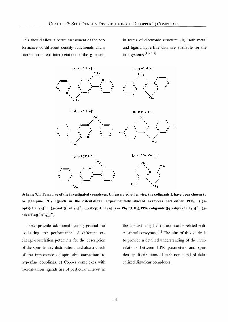
CHAPTER 7: SPIN-DENSITY DISTRIBUTIONS OF DICOPPER(I) COMPLEXES
114
This should allow a better assessment of the per-
formance of different density functionals and a
more transparent interpretation of the g-tensors
in terms of electronic structure. (b) Both metal
and ligand hyperfine data are available for the
title systems.[4, 5, 7, 8]
Scheme 7.1: Formulae of the investigated complexes. Unless noted otherwise, the coligands L have been chosen to
be phospine PH3 ligands in the calculations. Experimentally studied examples had either PPh3 ([(µ-
bptz)(CuL2)2]•+ , [(µ-bmtz)(CuL2)2]•+, [(µ-abcp)(CuL2)2]•+) or Ph2P(CH2)6PPh2 coligands ([(µ-abpy)(CuL2)2]•+, [(µ-
adcOtBu)(CuL2)2]•+).
These provide additional testing ground for
evaluating the performance of different ex-
change-correlation potentials for the description
of the spin-density distribution, and also a check
of the importance of spin-orbit corrections to
hyperfine couplings. c) Copper complexes with
radical-anion ligands are of particular interest in
the context of galactose oxidase or related radi-
cal-metalloenzymes.[2a] The aim of this study is
to provide a detailed understanding of the inter-
relations between EPR parameters and spin-
density distributions of such non-standard delo-
calized dinuclear complexes.
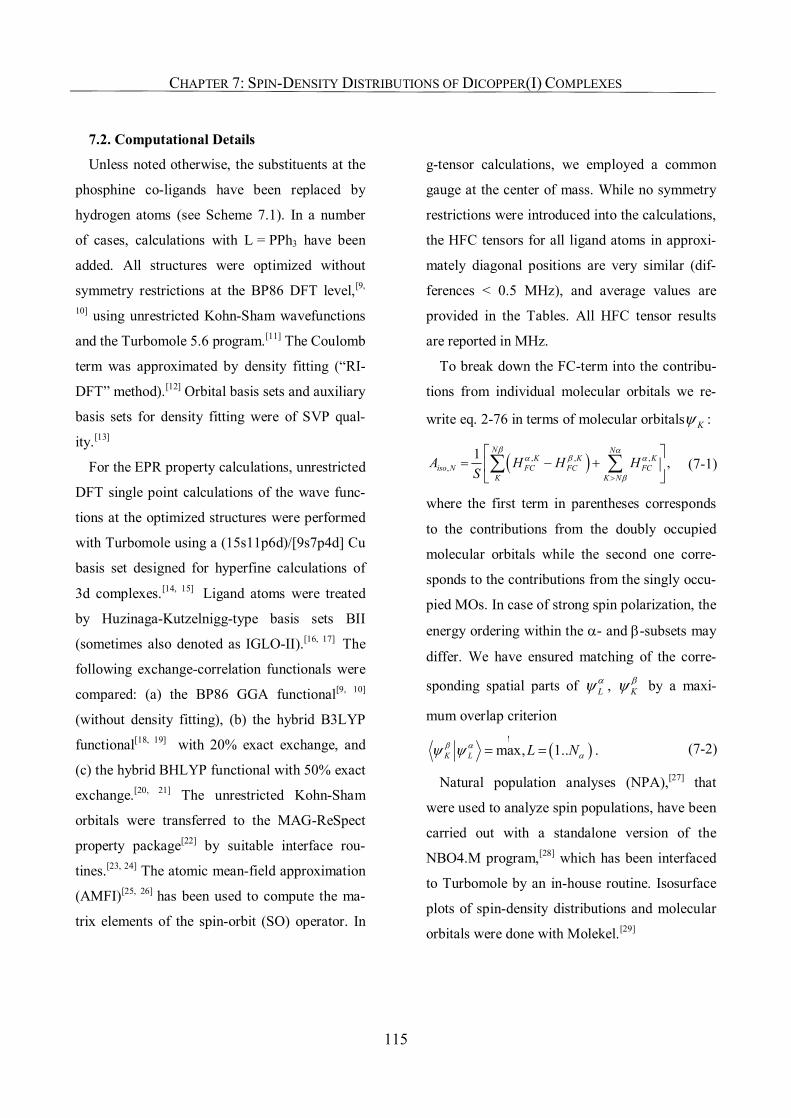
CHAPTER 7: SPIN-DENSITY DISTRIBUTIONS OF DICOPPER(I) COMPLEXES
115
7.2. Computational Details
Unless noted otherwise, the substituents at the
phosphine co-ligands have been replaced by
hydrogen atoms (see Scheme 7.1). In a number
of cases, calculations with L = PPh3 have been
added. All structures were optimized without
symmetry restrictions at the BP86 DFT level,[9,
10] using unrestricted Kohn-Sham wavefunctions
and the Turbomole 5.6 program.[11] The Coulomb
term was approximated by density fitting (“RI-
DFT” method).[12] Orbital basis sets and auxiliary
basis sets for density fitting were of SVP qual-
ity.[13]
For the EPR property calculations, unrestricted
DFT single point calculations of the wave func-
tions at the optimized structures were performed
with Turbomole using a (15s11p6d)/[9s7p4d] Cu
basis set designed for hyperfine calculations of
3d complexes.[14, 15] Ligand atoms were treated
by Huzinaga-Kutzelnigg-type basis sets BII
(sometimes also denoted as IGLO-II).[16, 17] The
following exchange-correlation functionals were
compared: (a) the BP86 GGA functional[9, 10]
(without density fitting), (b) the hybrid B3LYP
functional[18, 19] with 20% exact exchange, and
(c) the hybrid BHLYP functional with 50% exact
exchange.[20, 21] The unrestricted Kohn-Sham
orbitals were transferred to the MAG-ReSpect
property package[22] by suitable interface rou-
tines.[23, 24] The atomic mean-field approximation
(AMFI)[25, 26] has been used to compute the ma-
trix elements of the spin-orbit (SO) operator. In
g-tensor calculations, we employed a common
gauge at the center of mass. While no symmetry
restrictions were introduced into the calculations,
the HFC tensors for all ligand atoms in approxi-
mately diagonal positions are very similar (dif-
ferences < 0.5 MHz), and average values are
provided in the Tables. All HFC tensor results
are reported in MHz.
To break down the FC-term into the contribu-
tions from individual molecular orbitals we re-
write eq. 2-76 in terms of molecular orbitals Kψ :
( ), , ,,
1 ,N N
K K Kiso N FC FC FC
K K NA H H H
S
β αα β α
β>
= − +
∑ ∑ (7-1)
where the first term in parentheses corresponds
to the contributions from the doubly occupied
molecular orbitals while the second one corre-
sponds to the contributions from the singly occu-
pied MOs. In case of strong spin polarization, the
energy ordering within the α- and β-subsets may
differ. We have ensured matching of the corre-
sponding spatial parts of Lαψ , K
βψ by a maxi-
mum overlap criterion
( )!
max, 1..K L L Nβ ααψ ψ = = . (7-2)
Natural population analyses (NPA),[27] that
were used to analyze spin populations, have been
carried out with a standalone version of the
NBO4.M program,[28] which has been interfaced
to Turbomole by an in-house routine. Isosurface
plots of spin-density distributions and molecular
orbitals were done with Molekel.[29]
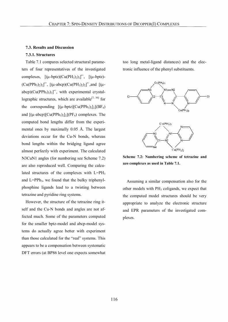
CHAPTER 7: SPIN-DENSITY DISTRIBUTIONS OF DICOPPER(I) COMPLEXES
116
7.3. Results and Discussion
7.3.1. Structures
Table 7.1 compares selected structural parame-
ters of four representatives of the investigated
complexes, [(µ-bptz)(Cu(PH3)2)2]•+, [(µ-bptz)-
(Cu(PPh3)2)2]•+, [(µ-abcp)(Cu(PH3)2)2]•+,and [(µ-
abcp)(Cu(PPh3)2)2]•+, with experimental crystal-
lographic structures, which are available[7, 30] for
the corresponding [(µ-bptz)[Cu(PPh3)2]2](BF4)
and [(µ-abcp)[Cu(PPh3)2]2](PF6) complexes. The
computed bond lengths differ from the experi-
mental ones by maximally 0.05 Å. The largest
deviations occur for the Cu-N bonds, whereas
bond lengths within the bridging ligand agree
almost perfectly with experiment. The calculated
N3CuN1 angles (for numbering see Scheme 7.2)
are also reproduced well. Comparing the calcu-
lated structures of the complexes with L=PH3
and L=PPh3, we found that the bulky triphenyl-
phosphine ligands lead to a twisting between
tetrazine and pyridine ring systems.
However, the structure of the tetrazine ring it-
self and the Cu-N bonds and angles are not af-
fected much. Some of the parameters computed
for the smaller bptz-model and abcp-model sys-
tems do actually agree better with experiment
than those calculated for the “real” systems. This
appears to be a compensation between systematic
DFT errors (at BP86 level one expects somewhat
too long metal-ligand distances) and the elec-
tronic influence of the phenyl substituents.
Scheme 7.2: Numbering scheme of tetrazine and
azo complexes as used in Table 7.1.
Assuming a similar compensation also for the
other models with PH3 coligands, we expect that
the computed model structures should be very
appropriate to analyze the electronic structure
and EPR parameters of the investigated com-
plexes.
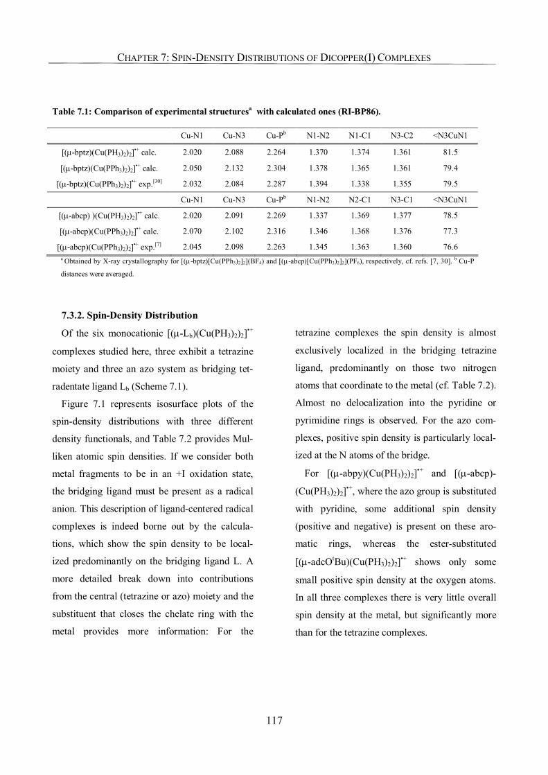
CHAPTER 7: SPIN-DENSITY DISTRIBUTIONS OF DICOPPER(I) COMPLEXES
117
Table 7.1: Comparison of experimental structuresa with calculated ones (RI-BP86).
Cu-N1 Cu-N3 Cu-Pb N1-N2 N1-C1 N3-C2 <N3CuN1
[(µ-bptz)(Cu(PH3)2)2]•+ calc. 2.020 2.088 2.264 1.370 1.374 1.361 81.5
[(µ-bptz)(Cu(PPh3)2)2]•+ calc. 2.050 2.132 2.304 1.378 1.365 1.361 79.4
[(µ-bptz)(Cu(PPh3)2)2]•+ exp.[30] 2.032 2.084 2.287 1.394 1.338 1.355 79.5
Cu-N1 Cu-N3 Cu-Pb N1-N2 N2-C1 N3-C1 <N3CuN1
[(µ-abcp) )(Cu(PH3)2)2]•+ calc. 2.020 2.091 2.269 1.337 1.369 1.377 78.5
[(µ-abcp)(Cu(PPh3)2)2]•+ calc. 2.070 2.102 2.316 1.346 1.368 1.376 77.3
[(µ-abcp)(Cu(PPh3)2)2]•+ exp.[7] 2.045 2.098 2.263 1.345 1.363 1.360 76.6 a Obtained by X-ray crystallography for [(µ-bptz)[Cu(PPh3)2]2](BF4) and [(µ-abcp)[Cu(PPh3)2]2](PF6), respectively, cf. refs. [7, 30]. b Cu-P
distances were averaged.
7.3.2. Spin-Density Distribution
Of the six monocationic [(µ-Lb)(Cu(PH3)2)2]•+
complexes studied here, three exhibit a tetrazine
moiety and three an azo system as bridging tet-
radentate ligand Lb (Scheme 7.1).
Figure 7.1 represents isosurface plots of the
spin-density distributions with three different
density functionals, and Table 7.2 provides Mul-
liken atomic spin densities. If we consider both
metal fragments to be in an +I oxidation state,
the bridging ligand must be present as a radical
anion. This description of ligand-centered radical
complexes is indeed borne out by the calcula-
tions, which show the spin density to be local-
ized predominantly on the bridging ligand L. A
more detailed break down into contributions
from the central (tetrazine or azo) moiety and the
substituent that closes the chelate ring with the
metal provides more information: For the
tetrazine complexes the spin density is almost
exclusively localized in the bridging tetrazine
ligand, predominantly on those two nitrogen
atoms that coordinate to the metal (cf. Table 7.2).
Almost no delocalization into the pyridine or
pyrimidine rings is observed. For the azo com-
plexes, positive spin density is particularly local-
ized at the N atoms of the bridge.
For [(µ-abpy)(Cu(PH3)2)2]•+ and [(µ-abcp)-
(Cu(PH3)2)2]•+, where the azo group is substituted
with pyridine, some additional spin density
(positive and negative) is present on these aro-
matic rings, whereas the ester-substituted
[(µ-adcOtBu)(Cu(PH3)2)2]•+ shows only some
small positive spin density at the oxygen atoms.
In all three complexes there is very little overall
spin density at the metal, but significantly more
than for the tetrazine complexes.
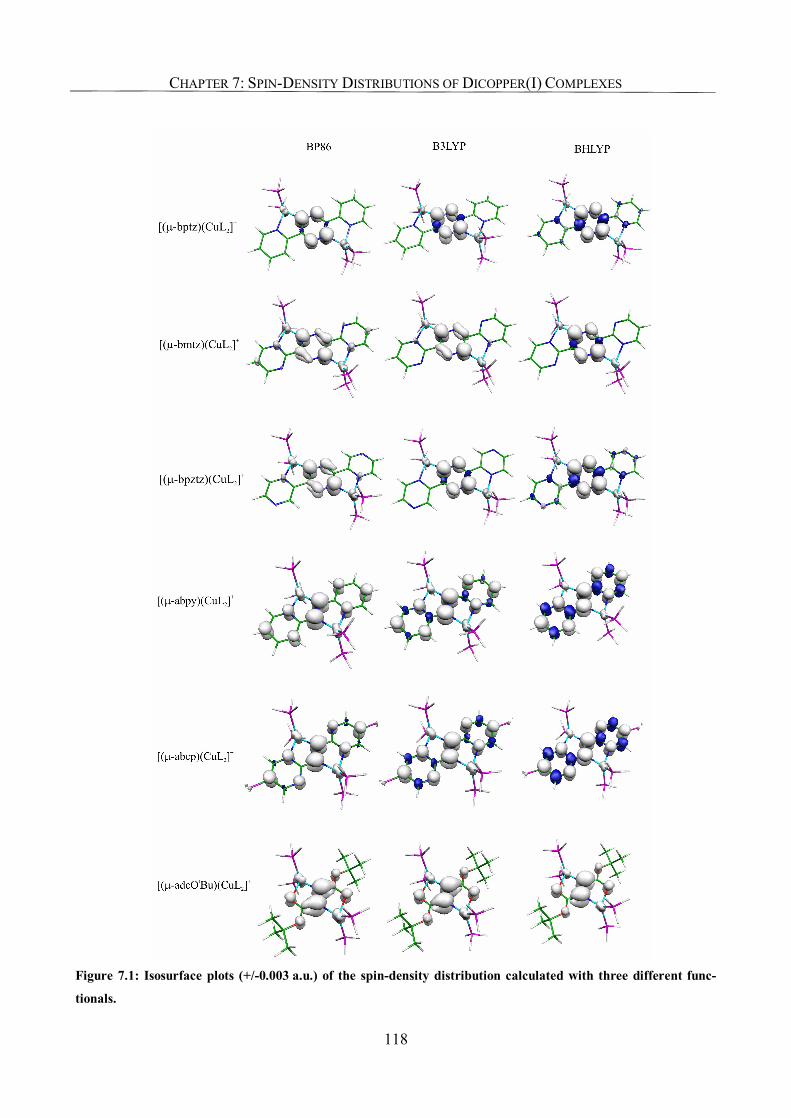
CHAPTER 7: SPIN-DENSITY DISTRIBUTIONS OF DICOPPER(I) COMPLEXES
118
Figure 7.1: Isosurface plots (+/-0.003 a.u.) of the spin-density distribution calculated with three different func-
tionals.
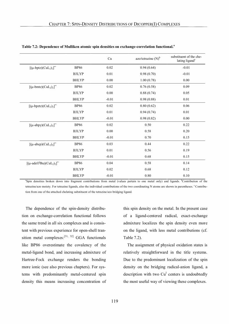
CHAPTER 7: SPIN-DENSITY DISTRIBUTIONS OF DICOPPER(I) COMPLEXES
119
Table 7.2: Dependence of Mulliken atomic spin densities on exchange-correlation functional.a
Cu azo/tetrazine (N)b substituent of the che-lating ligandc
BP86 0.02 0.94 (0.64) -0.01
B3LYP 0.01 0.98 (0.70) -0.01
[(µ-bptz)(CuL2)2]•+
BHLYP 0.00 1.00 (0.78) 0.00
BP86 0.02 0.76 (0.58) 0.09
B3LYP 0.00 0.88 (0.74) 0.05
[(µ-bmtz)(CuL2)2]•+
BHLYP -0.01 0.98 (0.88) 0.01
BP86 0.02 0.80 (0.62) 0.06
B3LYP 0.01 0.94 (0.74) 0.01
[(µ-bpztz)(CuL2)2]•+
BHLYP -0.01 0.98 (0.82) 0.00
BP86 0.02 0.50 0.22
B3LYP 0.00 0.58 0.20
[(µ-abpy)(CuL2)2]•+
BHLYP -0.01 0.70 0.15
BP86 0.03 0.44 0.22
B3LYP 0.01 0.56 0.19
[(µ-abcp)(CuL2)2]•+
BHLYP -0.01 0.68 0.15
BP86 0.04 0.58 0.14
B3LYP 0.02 0.68 0.12
[(µ-adcOtBu)(CuL2)2]•+
BHLYP -0.01 0.80 0.10 aSpin densities broken down into fragment contributions from metal (values pertain to one metal only) and ligands. bContribution of the
tetrazine/azo moiety. For tetrazine ligands, also the individual contributions of the two coordinating N atoms are shown in parentheses. c Contribu-
tion from one of the attached chelating substituent of the tetrazine/azo bridging ligand.
The dependence of the spin-density distribu-
tion on exchange-correlation functional follows
the same trend in all six complexes and is consis-
tent with previous experience for open-shell tran-
sition metal complexes:[31, 32] GGA functionals
like BP86 overestimate the covalency of the
metal-ligand bond, and increasing admixture of
Hartree-Fock exchange renders the bonding
more ionic (see also previous chapters). For sys-
tems with predominantly metal-centered spin
density this means increasing concentration of
this spin density on the metal. In the present case
of a ligand-centered radical, exact-exchange
admixture localizes the spin density even more
on the ligand, with less metal contributions (cf.
Table 7.2).
The assignment of physical oxidation states is
relatively straightforward in the title systems.
Due to the predominant localization of the spin
density on the bridging radical-anion ligand, a
description with two CuI centers is undoubtedly
the most useful way of viewing these complexes.
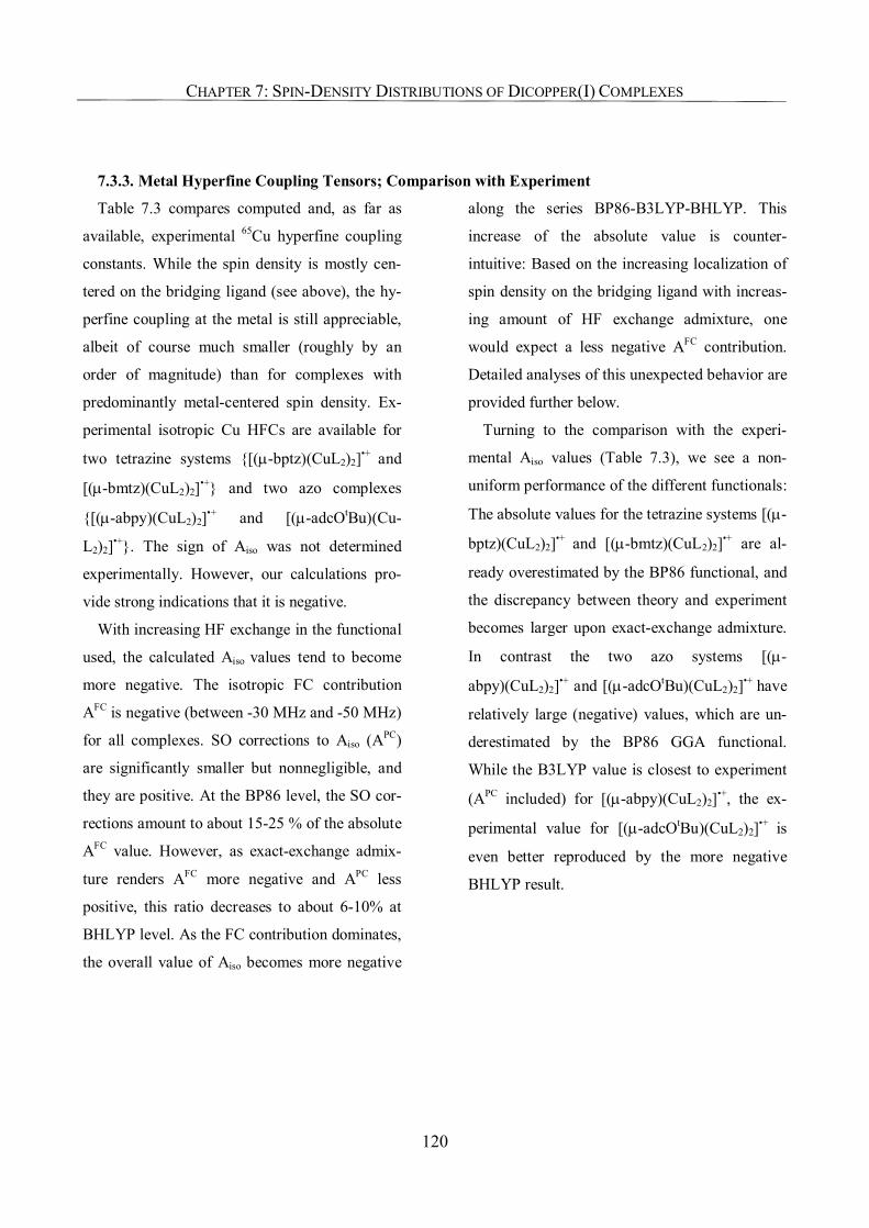
CHAPTER 7: SPIN-DENSITY DISTRIBUTIONS OF DICOPPER(I) COMPLEXES
120
7.3.3. Metal Hyperfine Coupling Tensors; Comparison with Experiment
Table 7.3 compares computed and, as far as
available, experimental 65Cu hyperfine coupling
constants. While the spin density is mostly cen-
tered on the bridging ligand (see above), the hy-
perfine coupling at the metal is still appreciable,
albeit of course much smaller (roughly by an
order of magnitude) than for complexes with
predominantly metal-centered spin density. Ex-
perimental isotropic Cu HFCs are available for
two tetrazine systems {[(µ-bptz)(CuL2)2]•+ and
[(µ-bmtz)(CuL2)2]•+} and two azo complexes
{[(µ-abpy)(CuL2)2]•+ and [(µ-adcOtBu)(Cu-
L2)2]•+}. The sign of Aiso was not determined
experimentally. However, our calculations pro-
vide strong indications that it is negative.
With increasing HF exchange in the functional
used, the calculated Aiso values tend to become
more negative. The isotropic FC contribution
AFC is negative (between -30 MHz and -50 MHz)
for all complexes. SO corrections to Aiso (APC)
are significantly smaller but nonnegligible, and
they are positive. At the BP86 level, the SO cor-
rections amount to about 15-25 % of the absolute
AFC value. However, as exact-exchange admix-
ture renders AFC more negative and APC less
positive, this ratio decreases to about 6-10% at
BHLYP level. As the FC contribution dominates,
the overall value of Aiso becomes more negative
along the series BP86-B3LYP-BHLYP. This
increase of the absolute value is counter-
intuitive: Based on the increasing localization of
spin density on the bridging ligand with increas-
ing amount of HF exchange admixture, one
would expect a less negative AFC contribution.
Detailed analyses of this unexpected behavior are
provided further below.
Turning to the comparison with the experi-
mental Aiso values (Table 7.3), we see a non-
uniform performance of the different functionals:
The absolute values for the tetrazine systems [(µ-
bptz)(CuL2)2]•+ and [(µ-bmtz)(CuL2)2]•+ are al-
ready overestimated by the BP86 functional, and
the discrepancy between theory and experiment
becomes larger upon exact-exchange admixture.
In contrast the two azo systems [(µ-
abpy)(CuL2)2]•+ and [(µ-adcOtBu)(CuL2)2]•+ have
relatively large (negative) values, which are un-
derestimated by the BP86 GGA functional.
While the B3LYP value is closest to experiment
(APC included) for [(µ-abpy)(CuL2)2]•+, the ex-
perimental value for [(µ-adcOtBu)(CuL2)2]•+ is
even better reproduced by the more negative
BHLYP result.
CHAPTER 7: SPIN-DENSITY DISTRIBUTIONS OF DICOPPER(I) COMPLEXES
121
Table 7.3: Computed and experimental 65Cu HFC tensors (in MHz) for the title complexes.
BP86 B3LYP BHLYP
Aiso -31.1 -33.2 -37.2
AFC -36.0 -36.6 -39.6
APC 4.9 3.4 2.3
Adip -27.5, 13.2, 14.3 -19.6, 9.4, 10.2 -13.5, 6.1, 7.4
Adip,2 4.1, -2.3, -1.8 2.9, -1.6, -1.4 2.1, -1.1, -1.0
[(µ-bptz)(CuL2)2]•+
Aiso (exp)10 (-) 21.24
Aiso -29.6 -34.8 -41.1
AFC -35.2 -39.0 -43.9
APC 5.6 4.1 2.8
Adip -29.0, 11.2, 17.9 -22.6, 8.7, 13.9 -15.9, 5.9, 9.9
Adip,2 4.7, -3.0, -1.6 3.5, -2.2, -1.3 2.4, -1.4, -1.0
[(µ-bmtz)(CuL2)2]•+
Aiso (exp)11 (-) 23.09
Aiso -31.7 -35.2 -38.9
AFC -37.7 -39.2 -41.5
APC 6.0 4.0 2.6
Adip -31.8, 15.6, 16.2 -22.6, 11.3, 11.3 -14.9, 7.0, 7.9
[(µ-bpztz)(CuL2)2]•+
Adip,2 5.0, -2.9, -2.1 3.5, -1.9, -1.6 2.3, -1.2, -1.1
Aiso -30.1 -34.4 -43.0
AFC -37.1 -39.6 -46.7
APC 7.0 5.2 3.6
Adip -33.0, 15.9, 17.1 -25.5, 12.3, 13.2 -18.6, 9.2, 9.4
Adip,2 5.3, -3.2, -2.1 4.0, -2.4, -1.6 2.6, -1.6, -1.1
[(µ-abpy)(CuL2)2]•+
Aiso (exp)10 (-) 36.43
Aiso -28.2 -33.3 -41.5
AFC -38.3 -40.5 -46.0
APC 10.1 7.3 4.4
Adip -40.7, 19.7, 21.0 -31.3, 15.1, 16.1 -20.9, 10.6, 10.3
[(µ-abcp)(CuL2)2]•+
Adip,2 7.7, -5.0, -2.7 5.8, -3.6, -2.2 3.5, -2.1, -1.4
Aiso -35.4 -40.0 -46.0
AFC -47.9 -48.6 -50.7
APC 12.4 8.6 4.7
Adip -49.3, 23.8, 25.5 -36.4, 17.3, 19.1 -22.3, 10.8, 11.5
Adip,2 10.6, -6.0, -4.6 -4.3, -3.7, 8.0 4.4, -2.3, -2.1
[(µ-adcOtBu) (CuL2)2]•+
Aiso (exp)10 (-) 46.29
CHAPTER 7: SPIN-DENSITY DISTRIBUTIONS OF DICOPPER(I) COMPLEXES
122
The dipolar hyperfine couplings exhibit almost
axial symmetry (with small deviations especially
for [(µ-bmtz) (Cu(PH3)2)2]•+). Again, the SO
contribution (Adip,2) is of opposite sign compared
to the primary nonrelativistic contribution (Adip)
and thus reduces the overall anisotropy some-
what. In contrast to the nonintuitive dependence
of Aiso on exchange-correlation functional (see
above), the absolute values of both Adip and Adip,2
decrease along the series BP86 > B3LYP >
BHLYP, in agreement with decreasing 3d spin
density upon increasing HF exchange admixture.
Consequently, the ratio between Adip,2 and Adip
remains roughly constant at ca. 15% in all cases.
7.3.4. Metal Hyperfine Couplings; Orbital Analysis
In view of the overall lower metal spin density
with increasing exact-exchange admixture (cf.
Figure 7.1), the unexpectedly more negative
isotropic metal hyperfine values along the same
series for all title complexes call for a closer
investigation. In Table 7.4, AFC is broken down
into individual molecular orbital contributions.
As has been discussed in detail earlier,35 core-
shell spin polarization contributions to the spin
density at the nucleus of a 3d complex arise from
a negative 2s and a somewhat smaller positive 3s
contribution. In the present examples, the rela-
tively small spin density on the metal renders
these contributions also relatively small, and due
to similar magnitude of the 2s and 3s contribu-
tions, the overall contribution to AFC from core-
shell spin polarization is only between -8 MHz
and -17 MHz at BP86 level. It decreases further
with exact-exchange admixture, to values be-
tween -3 MHz and -6 MHz at BHLYP level.
Thus, the core-shell spin polarization contribu-
tions become less negative, as expected, and they
do not account for the bulk of the computed AFC!
Instead, unexpectedly the bulk of the negative
contributions come from the spin polarization of
doubly occupied valence orbitals (summed up in
the “VS” column of Table 7.4). It is these VS
contributions that account for the more negative
AFC along the series BP86, B3LYP, BHLYP. The
predominant VS contributions arise from a few
(ca. 6-10) MOs, which have essentially σ-
symmetry with respect to the framework of the
bridging ligands’ π-system (that is, these MOs
have in-plane character within the bridging
ligand). All other orbitals contribute very little.
Figure 7.2 shows for one representative case,
[(µ-bmtz)(CuL2)2]•+, the spin density arising
from the superposition of these orbitals. The
picture may be viewed as the valence-shell spin-
polarization contribution to the overall spin-
density distribution (cf. Figure 7.1). With in-
creasing HF exchange admixture, the oscillation
of spin polarization within the ligand plane be-
comes more notable. At BHLYP level apprecia-
ble negative spin density contributions have de-
veloped around the metal centers. As the MOs
involved have some 4s-character on copper, this
leads to increasing negative spin density contri-
butions also at the metal nuclei, thus explaining
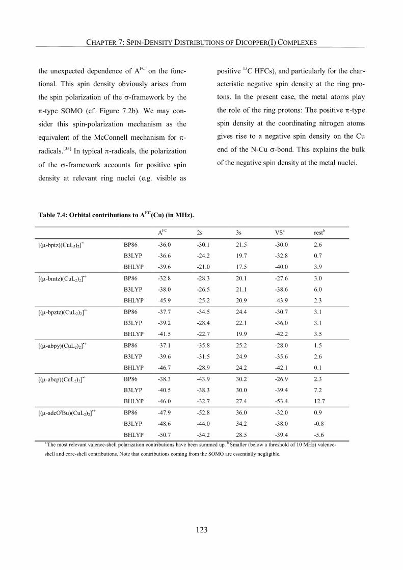
CHAPTER 7: SPIN-DENSITY DISTRIBUTIONS OF DICOPPER(I) COMPLEXES
123
the unexpected dependence of AFC on the func-
tional. This spin density obviously arises from
the spin polarization of the σ-framework by the
π-type SOMO (cf. Figure 7.2b). We may con-
sider this spin-polarization mechanism as the
equivalent of the McConnell mechanism for π-
radicals.[33] In typical π-radicals, the polarization
of the σ-framework accounts for positive spin
density at relevant ring nuclei (e.g. visible as
positive 13C HFCs), and particularly for the char-
acteristic negative spin density at the ring pro-
tons. In the present case, the metal atoms play
the role of the ring protons: The positive π-type
spin density at the coordinating nitrogen atoms
gives rise to a negative spin density on the Cu
end of the N-Cu σ-bond. This explains the bulk
of the negative spin density at the metal nuclei.
Table 7.4: Orbital contributions to AFC(Cu) (in MHz).
AFC 2s 3s VSa restb
BP86 -36.0 -30.1 21.5 -30.0 2.6
B3LYP -36.6 -24.2 19.7 -32.8 0.7
[(µ-bptz)(CuL2)2]•+
BHLYP -39.6 -21.0 17.5 -40.0 3.9
BP86 -32.8 -28.3 20.1 -27.6 3.0
B3LYP -38.0 -26.5 21.1 -38.6 6.0
[(µ-bmtz)(CuL2)2]•+
BHLYP -45.9 -25.2 20.9 -43.9 2.3
BP86 -37.7 -34.5 24.4 -30.7 3.1
B3LYP -39.2 -28.4 22.1 -36.0 3.1
[(µ-bpztz)(CuL2)2]•+
BHLYP -41.5 -22.7 19.9 -42.2 3.5
BP86 -37.1 -35.8 25.2 -28.0 1.5
B3LYP -39.6 -31.5 24.9 -35.6 2.6
[(µ-abpy)(CuL2)2]•+
BHLYP -46.7 -28.9 24.2 -42.1 0.1
BP86 -38.3 -43.9 30.2 -26.9 2.3
B3LYP -40.5 -38.3 30.0 -39.4 7.2
[(µ-abcp)(CuL2)2]•+
BHLYP -46.0 -32.7 27.4 -53.4 12.7
BP86 -47.9 -52.8 36.0 -32.0 0.9
B3LYP -48.6 -44.0 34.2 -38.0 -0.8
[(µ-adcOtBu)(CuL2)2]•+
BHLYP -50.7 -34.2 28.5 -39.4 -5.6 a The most relevant valence-shell polarization contributions have been summed up. b Smaller (below a threshold of 10 MHz) valence-
shell and core-shell contributions. Note that contributions coming from the SOMO are essentially negligible.
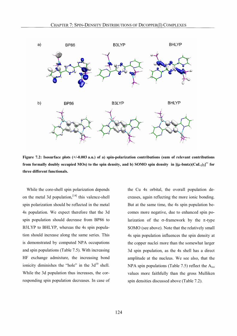
CHAPTER 7: SPIN-DENSITY DISTRIBUTIONS OF DICOPPER(I) COMPLEXES
124
Figure 7.2: Isosurface plots (+/-0.003 a.u.) of a) spin-polarization contributions (sum of relevant contributions
from formally doubly occupied MOs) to the spin density, and b) SOMO spin density in [(µ-bmtz)(CuL2)2]•+ for
three different functionals.
While the core-shell spin polarization depends
on the metal 3d population,[14] this valence-shell
spin polarization should be reflected in the metal
4s population. We expect therefore that the 3d
spin population should decrease from BP86 to
B3LYP to BHLYP, whereas the 4s spin popula-
tion should increase along the same series. This
is demonstrated by computed NPA occupations
and spin populations (Table 7.5). With increasing
HF exchange admixture, the increasing bond
ionicity diminishes the “hole” in the 3d10 shell.
While the 3d population thus increases, the cor-
responding spin population decreases. In case of
the Cu 4s orbital, the overall population de-
creases, again reflecting the more ionic bonding.
But at the same time, the 4s spin population be-
comes more negative, due to enhanced spin po-
larization of the σ-framework by the π-type
SOMO (see above). Note that the relatively small
4s spin population influences the spin density at
the copper nuclei more than the somewhat larger
3d spin population, as the 4s shell has a direct
amplitude at the nucleus. We see also, that the
NPA spin populations (Table 7.5) reflect the Aiso
values more faithfully than the gross Mulliken
spin densities discussed above (Table 7.2).
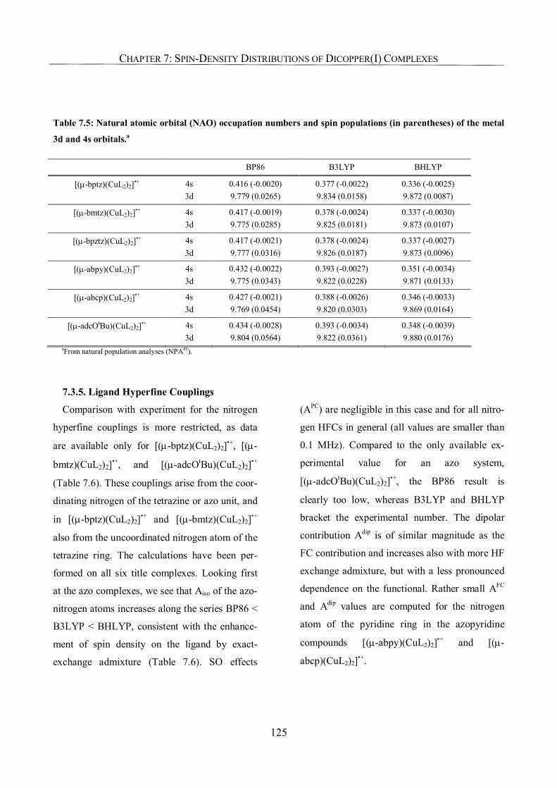
CHAPTER 7: SPIN-DENSITY DISTRIBUTIONS OF DICOPPER(I) COMPLEXES
125
Table 7.5: Natural atomic orbital (NAO) occupation numbers and spin populations (in parentheses) of the metal
3d and 4s orbitals.a
BP86 B3LYP BHLYP
[(µ-bptz)(CuL2)2]•+ 4s 3d
0.416 (-0.0020) 9.779 (0.0265)
0.377 (-0.0022) 9.834 (0.0158)
0.336 (-0.0025) 9.872 (0.0087)
[(µ-bmtz)(CuL2)2]•+ 4s 3d
0.417 (-0.0019) 9.775 (0.0285)
0.378 (-0.0024) 9.825 (0.0181)
0.337 (-0.0030) 9.873 (0.0107)
[(µ-bpztz)(CuL2)2]•+ 4s 3d
0.417 (-0.0021) 9.777 (0.0316)
0.378 (-0.0024) 9.826 (0.0187)
0.337 (-0.0027) 9.873 (0.0096)
[(µ-abpy)(CuL2)2]•+ 4s 3d
0.432 (-0.0022) 9.775 (0.0343)
0.393 (-0.0027) 9.822 (0.0228)
0.351 (-0.0034) 9.871 (0.0133)
[(µ-abcp)(CuL2)2]•+ 4s 3d
0.427 (-0.0021) 9.769 (0.0454)
0.388 (-0.0026) 9.820 (0.0303)
0.346 (-0.0033) 9.869 (0.0164)
[(µ-adcOtBu)(CuL2)2]•+ 4s 3d
0.434 (-0.0028) 9.804 (0.0564)
0.393 (-0.0034) 9.822 (0.0361)
0.348 (-0.0039) 9.880 (0.0176)
aFrom natural population analyses (NPA45).
7.3.5. Ligand Hyperfine Couplings
Comparison with experiment for the nitrogen
hyperfine couplings is more restricted, as data
are available only for [(µ-bptz)(CuL2)2]•+, [(µ-
bmtz)(CuL2)2]•+, and [(µ-adcOtBu)(CuL2)2]•+
(Table 7.6). These couplings arise from the coor-
dinating nitrogen of the tetrazine or azo unit, and
in [(µ-bptz)(CuL2)2]•+ and [(µ-bmtz)(CuL2)2]•+
also from the uncoordinated nitrogen atom of the
tetrazine ring. The calculations have been per-
formed on all six title complexes. Looking first
at the azo complexes, we see that Aiso of the azo-
nitrogen atoms increases along the series BP86 <
B3LYP < BHLYP, consistent with the enhance-
ment of spin density on the ligand by exact-
exchange admixture (Table 7.6). SO effects
(APC) are negligible in this case and for all nitro-
gen HFCs in general (all values are smaller than
0.1 MHz). Compared to the only available ex-
perimental value for an azo system,
[(µ-adcOtBu)(CuL2)2]•+, the BP86 result is
clearly too low, whereas B3LYP and BHLYP
bracket the experimental number. The dipolar
contribution Adip is of similar magnitude as the
FC contribution and increases also with more HF
exchange admixture, but with a less pronounced
dependence on the functional. Rather small AFC
and Adip values are computed for the nitrogen
atom of the pyridine ring in the azopyridine
compounds [(µ-abpy)(CuL2)2]•+ and [(µ-
abcp)(CuL2)2]•+.
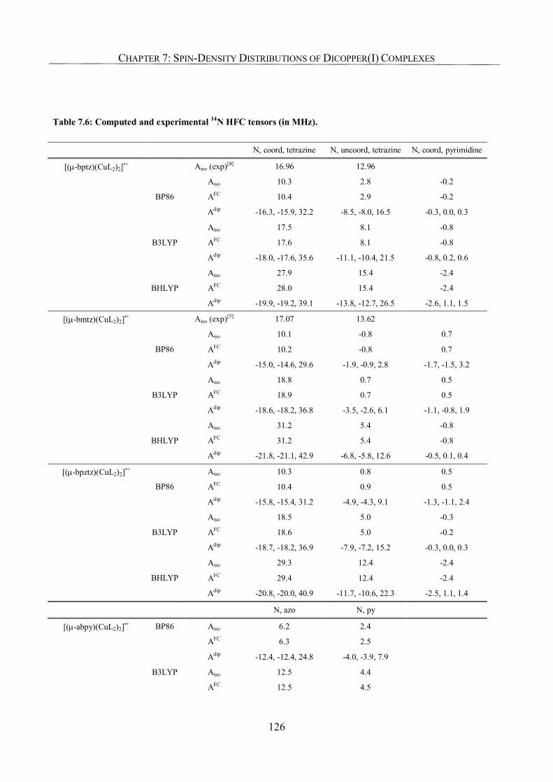
CHAPTER 7: SPIN-DENSITY DISTRIBUTIONS OF DICOPPER(I) COMPLEXES
126
Table 7.6: Computed and experimental 14N HFC tensors (in MHz).
N, coord, tetrazine N, uncoord, tetrazine N, coord, pyrimidine
Aiso (exp)[4] 16.96 12.96
Aiso 10.3 2.8 -0.2
AFC 10.4 2.9 -0.2 BP86
Adip -16.3, -15.9, 32.2 -8.5, -8.0, 16.5 -0.3, 0.0, 0.3
Aiso 17.5 8.1 -0.8
AFC 17.6 8.1 -0.8 B3LYP
Adip -18.0, -17.6, 35.6 -11.1, -10.4, 21.5 -0.8, 0.2, 0.6
Aiso 27.9 15.4 -2.4
AFC 28.0 15.4 -2.4
[(µ-bptz)(CuL2)2]•+
BHLYP
Adip -19.9, -19.2, 39.1 -13.8, -12.7, 26.5 -2.6, 1.1, 1.5
Aiso (exp)[5] 17.07 13.62
Aiso 10.1 -0.8 0.7
AFC 10.2 -0.8 0.7 BP86
Adip -15.0, -14.6, 29.6 -1.9, -0.9, 2.8 -1.7, -1.5, 3.2
Aiso 18.8 0.7 0.5
AFC 18.9 0.7 0.5 B3LYP
Adip -18.6, -18.2, 36.8 -3.5, -2.6, 6.1 -1.1, -0.8, 1.9
Aiso 31.2 5.4 -0.8
AFC 31.2 5.4 -0.8
[(µ-bmtz)(CuL2)2]•+
BHLYP
Adip -21.8, -21.1, 42.9 -6.8, -5.8, 12.6 -0.5, 0.1, 0.4
Aiso 10.3 0.8 0.5
AFC 10.4 0.9 0.5 BP86
Adip -15.8, -15.4, 31.2 -4.9, -4.3, 9.1 -1.3, -1.1, 2.4
Aiso 18.5 5.0 -0.3
AFC 18.6 5.0 -0.2 B3LYP
Adip -18.7, -18.2, 36.9 -7.9, -7.2, 15.2 -0.3, 0.0, 0.3
Aiso 29.3 12.4 -2.4
AFC 29.4 12.4 -2.4
[(µ-bpztz)(CuL2)2]•+
BHLYP
Adip -20.8, -20.0, 40.9 -11.7, -10.6, 22.3 -2.5, 1.1, 1.4
N, azo N, py
BP86 Aiso 6.2 2.4
AFC 6.3 2.5
Adip -12.4, -12.4, 24.8 -4.0, -3.9, 7.9
B3LYP Aiso 12.5 4.4
[(µ-abpy)(CuL2)2]•+
AFC 12.5 4.5
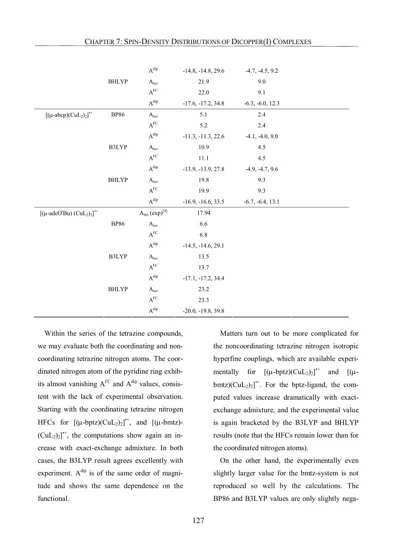
CHAPTER 7: SPIN-DENSITY DISTRIBUTIONS OF DICOPPER(I) COMPLEXES
127
Adip -14.8, -14.8, 29.6 -4.7, -4.5, 9.2
BHLYP Aiso 21.9 9.0
AFC 22.0 9.1
Adip -17.6, -17.2, 34.8 -6.3, -6.0, 12.3
BP86 Aiso 5.1 2.4
AFC 5.2 2.4
Adip -11.3, -11.3, 22.6 -4.1, -4.0, 8.0
B3LYP Aiso 10.9 4.5
AFC 11.1 4.5
Adip -13.9, -13.9, 27.8 -4.9, -4.7, 9.6
BHLYP Aiso 19.8 9.3
AFC 19.9 9.3
[(µ-abcp)(CuL2)2]•+
Adip -16.9, -16.6, 33.5 -6.7, -6.4, 13.1
Aiso (exp)[4] 17.94
BP86 Aiso 6.6
AFC 6.8
Adip -14.5, -14.6, 29.1
B3LYP Aiso 13.5
AFC 13.7
Adip -17.1, -17.2, 34.4
BHLYP Aiso 23.2
AFC 23.3
[(µ-adcOtBu) (CuL2)2]•+
Adip -20.0, -19.8, 39.8
Within the series of the tetrazine compounds,
we may evaluate both the coordinating and non-
coordinating tetrazine nitrogen atoms. The coor-
dinated nitrogen atom of the pyridine ring exhib-
its almost vanishing AFC and Adip values, consis-
tent with the lack of experimental observation.
Starting with the coordinating tetrazine nitrogen
HFCs for [(µ-bptz)(CuL2)2]•+, and [(µ-bmtz)-
(CuL2)2]•+, the computations show again an in-
crease with exact-exchange admixture. In both
cases, the B3LYP result agrees excellently with
experiment. Adip is of the same order of magni-
tude and shows the same dependence on the
functional.
Matters turn out to be more complicated for
the noncoordinating tetrazine nitrogen isotropic
hyperfine couplings, which are available experi-
mentally for [(µ-bptz)(CuL2)2]•+ and [(µ-
bmtz)(CuL2)2]•+. For the bptz-ligand, the com-
puted values increase dramatically with exact-
exchange admixture, and the experimental value
is again bracketed by the B3LYP and BHLYP
results (note that the HFCs remain lower than for
the coordinated nitrogen atoms).
On the other hand, the experimentally even
slightly larger value for the bmtz-system is not
reproduced so well by the calculations. The
BP86 and B3LYP values are only slightly nega-
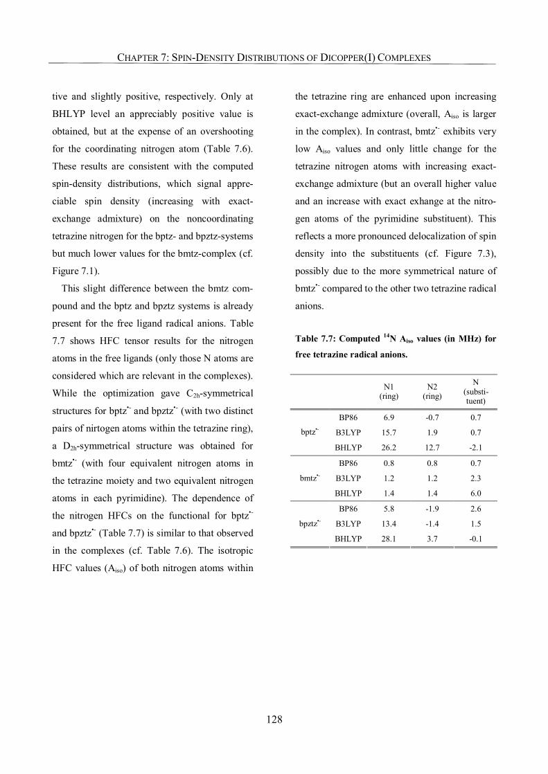
CHAPTER 7: SPIN-DENSITY DISTRIBUTIONS OF DICOPPER(I) COMPLEXES
128
tive and slightly positive, respectively. Only at
BHLYP level an appreciably positive value is
obtained, but at the expense of an overshooting
for the coordinating nitrogen atom (Table 7.6).
These results are consistent with the computed
spin-density distributions, which signal appre-
ciable spin density (increasing with exact-
exchange admixture) on the noncoordinating
tetrazine nitrogen for the bptz- and bpztz-systems
but much lower values for the bmtz-complex (cf.
Figure 7.1).
This slight difference between the bmtz com-
pound and the bptz and bpztz systems is already
present for the free ligand radical anions. Table
7.7 shows HFC tensor results for the nitrogen
atoms in the free ligands (only those N atoms are
considered which are relevant in the complexes).
While the optimization gave C2h-symmetrical
structures for bptz•- and bpztz•- (with two distinct
pairs of nirtogen atoms within the tetrazine ring),
a D2h-symmetrical structure was obtained for
bmtz•- (with four equivalent nitrogen atoms in
the tetrazine moiety and two equivalent nitrogen
atoms in each pyrimidine). The dependence of
the nitrogen HFCs on the functional for bptz•-
and bpztz•- (Table 7.7) is similar to that observed
in the complexes (cf. Table 7.6). The isotropic
HFC values (Aiso) of both nitrogen atoms within
the tetrazine ring are enhanced upon increasing
exact-exchange admixture (overall, Aiso is larger
in the complex). In contrast, bmtz•- exhibits very
low Aiso values and only little change for the
tetrazine nitrogen atoms with increasing exact-
exchange admixture (but an overall higher value
and an increase with exact exhange at the nitro-
gen atoms of the pyrimidine substituent). This
reflects a more pronounced delocalization of spin
density into the substituents (cf. Figure 7.3),
possibly due to the more symmetrical nature of
bmtz•- compared to the other two tetrazine radical
anions.
Table 7.7: Computed 14N Aiso values (in MHz) for
free tetrazine radical anions.
N1 (ring)
N2 (ring)
N (substi-tuent)
BP86 6.9 -0.7 0.7
B3LYP 15.7 1.9 0.7 bptz•-
BHLYP 26.2 12.7 -2.1
BP86 0.8 0.8 0.7
B3LYP 1.2 1.2 2.3 bmtz•-
BHLYP 1.4 1.4 6.0
BP86 5.8 -1.9 2.6
B3LYP 13.4 -1.4 1.5 bpztz•-
BHLYP 28.1 3.7 -0.1
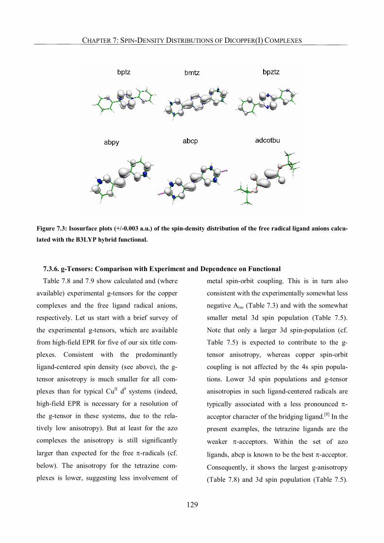
CHAPTER 7: SPIN-DENSITY DISTRIBUTIONS OF DICOPPER(I) COMPLEXES
129
Figure 7.3: Isosurface plots (+/-0.003 a.u.) of the spin-density distribution of the free radical ligand anions calcu-
lated with the B3LYP hybrid functional.
7.3.6. g-Tensors: Comparison with Experiment and Dependence on Functional
Table 7.8 and 7.9 show calculated and (where
available) experimental g-tensors for the copper
complexes and the free ligand radical anions,
respectively. Let us start with a brief survey of
the experimental g-tensors, which are available
from high-field EPR for five of our six title com-
plexes. Consistent with the predominantly
ligand-centered spin density (see above), the g-
tensor anisotropy is much smaller for all com-
plexes than for typical CuII d9 systems (indeed,
high-field EPR is necessary for a resolution of
the g-tensor in these systems, due to the rela-
tively low anisotropy). But at least for the azo
complexes the anisotropy is still significantly
larger than expected for the free π-radicals (cf.
below). The anisotropy for the tetrazine com-
plexes is lower, suggesting less involvement of
metal spin-orbit coupling. This is in turn also
consistent with the experimentally somewhat less
negative Aiso (Table 7.3) and with the somewhat
smaller metal 3d spin population (Table 7.5).
Note that only a larger 3d spin-population (cf.
Table 7.5) is expected to contribute to the g-
tensor anisotropy, whereas copper spin-orbit
coupling is not affected by the 4s spin popula-
tions. Lower 3d spin populations and g-tensor
anisotropies in such ligand-centered radicals are
typically associated with a less pronounced π-
acceptor character of the bridging ligand.[8] In the
present examples, the tetrazine ligands are the
weaker π-acceptors. Within the set of azo
ligands, abcp is known to be the best π-acceptor.
Consequently, it shows the largest g-anisotropy
(Table 7.8) and 3d spin population (Table 7.5).
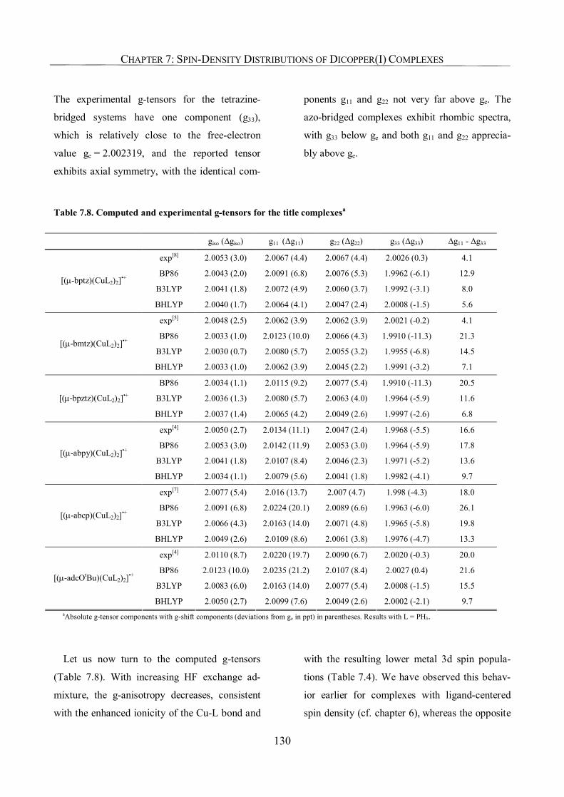
CHAPTER 7: SPIN-DENSITY DISTRIBUTIONS OF DICOPPER(I) COMPLEXES
130
The experimental g-tensors for the tetrazine-
bridged systems have one component (g33),
which is relatively close to the free-electron
value ge = 2.002319, and the reported tensor
exhibits axial symmetry, with the identical com-
ponents g11 and g22 not very far above ge. The
azo-bridged complexes exhibit rhombic spectra,
with g33 below ge and both g11 and g22 apprecia-
bly above ge.
Table 7.8. Computed and experimental g-tensors for the title complexesa
giso (Δgiso) g11 (Δg11) g22 (Δg22) g33 (Δg33) Δg11 - Δg33
exp[8] 2.0053 (3.0) 2.0067 (4.4) 2.0067 (4.4) 2.0026 (0.3) 4.1
BP86 2.0043 (2.0) 2.0091 (6.8) 2.0076 (5.3) 1.9962 (-6.1) 12.9
B3LYP 2.0041 (1.8) 2.0072 (4.9) 2.0060 (3.7) 1.9992 (-3.1) 8.0 [(µ-bptz)(CuL2)2]•+
BHLYP 2.0040 (1.7) 2.0064 (4.1) 2.0047 (2.4) 2.0008 (-1.5) 5.6
exp[5] 2.0048 (2.5) 2.0062 (3.9) 2.0062 (3.9) 2.0021 (-0.2) 4.1
BP86 2.0033 (1.0) 2.0123 (10.0) 2.0066 (4.3) 1.9910 (-11.3) 21.3
B3LYP 2.0030 (0.7) 2.0080 (5.7) 2.0055 (3.2) 1.9955 (-6.8) 14.5 [(µ-bmtz)(CuL2)2]•+
BHLYP 2.0033 (1.0) 2.0062 (3.9) 2.0045 (2.2) 1.9991 (-3.2) 7.1
BP86 2.0034 (1.1) 2.0115 (9.2) 2.0077 (5.4) 1.9910 (-11.3) 20.5
B3LYP 2.0036 (1.3) 2.0080 (5.7) 2.0063 (4.0) 1.9964 (-5.9) 11.6 [(µ-bpztz)(CuL2)2]•+
BHLYP 2.0037 (1.4) 2.0065 (4.2) 2.0049 (2.6) 1.9997 (-2.6) 6.8
exp[4] 2.0050 (2.7) 2.0134 (11.1) 2.0047 (2.4) 1.9968 (-5.5) 16.6
BP86 2.0053 (3.0) 2.0142 (11.9) 2.0053 (3.0) 1.9964 (-5.9) 17.8
B3LYP 2.0041 (1.8) 2.0107 (8.4) 2.0046 (2.3) 1.9971 (-5.2) 13.6 [(µ-abpy)(CuL2)2]•+
BHLYP 2.0034 (1.1) 2.0079 (5.6) 2.0041 (1.8) 1.9982 (-4.1) 9.7
exp[7] 2.0077 (5.4) 2.016 (13.7) 2.007 (4.7) 1.998 (-4.3) 18.0
BP86 2.0091 (6.8) 2.0224 (20.1) 2.0089 (6.6) 1.9963 (-6.0) 26.1
B3LYP 2.0066 (4.3) 2.0163 (14.0) 2.0071 (4.8) 1.9965 (-5.8) 19.8 [(µ-abcp)(CuL2)2]•+
BHLYP 2.0049 (2.6) 2.0109 (8.6) 2.0061 (3.8) 1.9976 (-4.7) 13.3
exp[4] 2.0110 (8.7) 2.0220 (19.7) 2.0090 (6.7) 2.0020 (-0.3) 20.0
BP86 2.0123 (10.0) 2.0235 (21.2) 2.0107 (8.4) 2.0027 (0.4) 21.6
B3LYP 2.0083 (6.0) 2.0163 (14.0) 2.0077 (5.4) 2.0008 (-1.5) 15.5 [(µ-adcOtBu)(CuL2)2]•+
BHLYP 2.0050 (2.7) 2.0099 (7.6) 2.0049 (2.6) 2.0002 (-2.1) 9.7 aAbsolute g-tensor components with g-shift components (deviations from ge in ppt) in parentheses. Results with L = PH3.
Let us now turn to the computed g-tensors
(Table 7.8). With increasing HF exchange ad-
mixture, the g-anisotropy decreases, consistent
with the enhanced ionicity of the Cu-L bond and
with the resulting lower metal 3d spin popula-
tions (Table 7.4). We have observed this behav-
ior earlier for complexes with ligand-centered
spin density (cf. chapter 6), whereas the opposite
CHAPTER 7: SPIN-DENSITY DISTRIBUTIONS OF DICOPPER(I) COMPLEXES
131
trend holds for metal-centered spin.[34, 35] The
overall agreement with experiment is generally
better for the present Cu complexes than for pre-
vious works on 4d or 5d ligand-centered sys-
tems.[3, 31] For the azo complexes, both BP86 and
B3LYP results may be considered to agree well
with experiment for all three tensor components
and thus also for the anisotropy. The BHLYP
results exhibit too low g11 and g22 and thus un-
derestimate the g-anisotropy.
For the two tetrazine complexes [(µ-
bptz)(CuL2)2]•+ and [(µ-bmtz)(CuL2)2]•+, for
which g-tensor data are available, the agreement
between theory and experiment is less favorable:
Δg33 is computed too negative at BP86 level and
slowly moves towards better agreement with the
very small absolute experimental values upon
going towards BHLYP. Also, the axial symmetry
(i.e. g11 = g22) of the experimental data is not
reproduced by the calculations, which exhibit a
splitting of ca. 1-5 ppt between the two larger
components, depending on system and functional
(Table 7.8). Comparison of the average of the
computed g11 and g22 values with the experimen-
tal value would suggest again best agreement
with experiment at the B3LYP level. On the
other hand, the less negative g33 brings the g-
anisotropy into better agreement with experiment
at BHLYP level. However, it appears possible
that the g11-g22 asymmetry was just too small to
be resolved under the experimental conditions.
We can also not exclude that the discrepancy
between theory and experiment for g33 may be
partly due to an insufficient magnetic-field cali-
bration under the experimental setup. One should
thus probably not overinterpret the discrepancies
between theory and experiment for the two
tetrazine title complexes.
Table 7.9 shows computed g-shift tensors for
the free ligand radical anions. As one might ex-
pect for typical organic π-radicals, the anisot-
ropies are much reduced compared to the com-
plexes, with g33 (the component perpendicular to
the molecular plane) near ge and g11 and g22
about 2-7 ppt above ge, depending on the spin
densities on nitrogen centers, which are respon-
sible for the predominant spin-orbit contributions
in the free radical anions. The much less pro-
nounced dependence of the computed g-tensors
on exchange-correlation functional for the free
ligands compared to the complexes (cf. Table
7.8) is notable. This confirms the above discus-
sion of the dependence of metal-ligand cova-
lency on the functional, and of the influence of
this covalency on the metal spin density. For
three cases (bmtz•-, abcp•-, and abpy•-), experi-
mental giso values are available. The only
tetrazine system, bmtz•-, appears to be repro-
duced most poorly by the calculations, whereas
the two values of the azo-compounds exhibit
reasonable agreement between theory and ex-
periment. It is furthermore clear that the azo sys-
tems exhibit more rhombic g-tensors, with larger
g11, than the tetrazine radical anions. This must
reflect appreciable spin density on the nitrogen
atoms of the azo bridge. The trends of g-tensor
anisotropy in the complexes (Table 7.8) do not
generally follow those of the free radical anions.
This indicates the importance of metal-ligand
interactions (related to the π-acceptor character
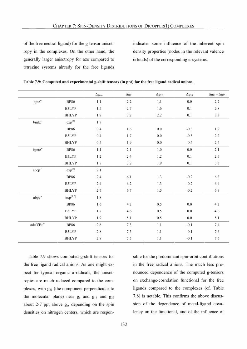
CHAPTER 7: SPIN-DENSITY DISTRIBUTIONS OF DICOPPER(I) COMPLEXES
132
of the free neutral ligand) for the g-tensor anisot-
ropy in the complexes. On the other hand, the
generally larger anisotropy for azo compared to
tetrazine systems already for the free ligands
indicates some influence of the inherent spin
density properties (nodes in the relevant valence
orbitals) of the corresponding π-systems.
Table 7.9: Computed and experimental g-shift tensors (in ppt) for the free ligand radical anions.
Δgiso Δg11 Δg22 Δg33 Δg11 - Δg33
BP86 1.1 2.2 1.1 0.0 2.2
B3LYP 1.5 2.7 1.6 0.1 2.8
bptz•-
BHLYP 1.8 3.2 2.2 0.1 3.3
exp[5] 1.7
BP86 0.4 1.6 0.0 -0.3 1.9
B3LYP 0.4 1.7 0.0 -0.5 2.2
bmtz•-
BHLYP 0.5 1.9 0.0 -0.5 2.4
BP86 1.1 2.1 1.0 0.0 2.1
B3LYP 1.2 2.4 1.2 0.1 2.5
bpztz•-
BHLYP 1.7 3.2 1.9 0.1 3.3
exp[3] 2.1
BP86 2.4 6.1 1.3 -0.2 6.3
B3LYP 2.4 6.2 1.3 -0.2 6.4
abcp •-
BHLYP 2.7 6.7 1.5 -0.2 6.9
exp[3, 7] 1.8
BP86 1.6 4.2 0.5 0.0 4.2
B3LYP 1.7 4.6 0.5 0.0 4.6
abpy•-
BHLYP 1.9 5.1 0.5 0.0 5.1
BP86 2.8 7.3 1.1 -0.1 7.4
B3LYP 2.8 7.5 1.1 -0.1 7.6
adcOtBu•-
BHLYP 2.8 7.5 1.1 -0.1 7.6
Table 7.9 shows computed g-shift tensors for
the free ligand radical anions. As one might ex-
pect for typical organic π-radicals, the anisot-
ropies are much reduced compared to the com-
plexes, with g33 (the component perpendicular to
the molecular plane) near ge and g11 and g22
about 2-7 ppt above ge, depending on the spin
densities on nitrogen centers, which are respon-
sible for the predominant spin-orbit contributions
in the free radical anions. The much less pro-
nounced dependence of the computed g-tensors
on exchange-correlation functional for the free
ligands compared to the complexes (cf. Table
7.8) is notable. This confirms the above discus-
sion of the dependence of metal-ligand cova-
lency on the functional, and of the influence of
CHAPTER 7: SPIN-DENSITY DISTRIBUTIONS OF DICOPPER(I) COMPLEXES
133
this covalency on the metal spin density. For
three cases (bmtz•-, abcp•-, and abpy•-), experi-
mental giso values are available. The only
tetrazine system, bmtz•-, appears to be repro-
duced most poorly by the calculations, whereas
the two values of the azo compounds exhibit
reasonable agreement between theory and ex-
periment. It is furthermore clear that the azo sys-
tems exhibit more rhombic g-tensors, with larger
g11, than the tetrazine radical anions. This must
reflect appreciable spin density on the nitrogen
atoms of the azo bridge. The trends of g-tensor
anisotropy in the complexes (Table 7.8) do not
generally follow those of the free radical anions.
This indicates the importance of metal-ligand
interactions (related to the π-acceptor character
of the free neutral ligand) for the g-tensor anisot-
ropy in the complexes. On the other hand, the
generally larger anisotropy for azo compared to
tetrazine systems already for the free ligands
indicates some influence of the inherent spin
density properties (nodes in the relevant valence
orbitals) of the corresponding π-systems.
7.3.7. Effect of the Phosphine Co-Ligands, Comparison of L = PH3 and L = PPh3
As indicated by the structural results (see
above), the choice of L=PH3 appears to be a rea-
sonable one, partly due to a compensation be-
tween computational errors and substituent ef-
fects on structures. To nevertheless obtain an
impression of the actual influence of more realis-
tically substituted phosphine co-ligands, we have
carried out additional calculations with
triphenylphosphine ligands for two tetrazine
complexes [(µ-bptz)(CuL2)2]•+, [(µ-bmtz)-
(CuL2)2]•+ and one azo complex [(µ-abcp)-
CuL2)2]•+. This choice was based on the fact that
these three systems indeed were studied experi-
mentally with PPh3 coligands. Due to system
size, we restrict the calculations to one computa-
tional level, using the BP86 GGA functional.
Results of such comparisons for all relevant EPR
parameters are provided in Table 7.10. We will
not compare to experiment at this computational
level but refer the reader to the corresponding
experimental values in Tables 7.3, 7.6, and 7.8
above.
Starting with metal HFCs, we see slightly less
negative Aiso values upon replacing PH3 by PPh3.
For the two tetrazine complexes this is due to a
less negative FC term, whereas a more positive
pseudocontact term overcompensates the slightly
more negative contact term for the azo complex
(Table 7.10). The dipolar coupling constants
exhibit an unclear trend, with enhancement for
the azo complex [(µ-abcp)Cu(PPh3)2)2]•+, de-
crease for [(µ-bmtz)(CuL2)2]•+ and relatively
little change for [(µ-bptz)(CuL2)2]•+. The HFC
rhombicity is increased upon substitution. This
probably reflects the slightly twisted ring planes
in the complexes with triphenylphosphine coli-
gands (see above). Overall these results indicate
that the spin density at the metal is influenced
only moderately and in a subtle fashion by the
presence of the phenyl substituents.
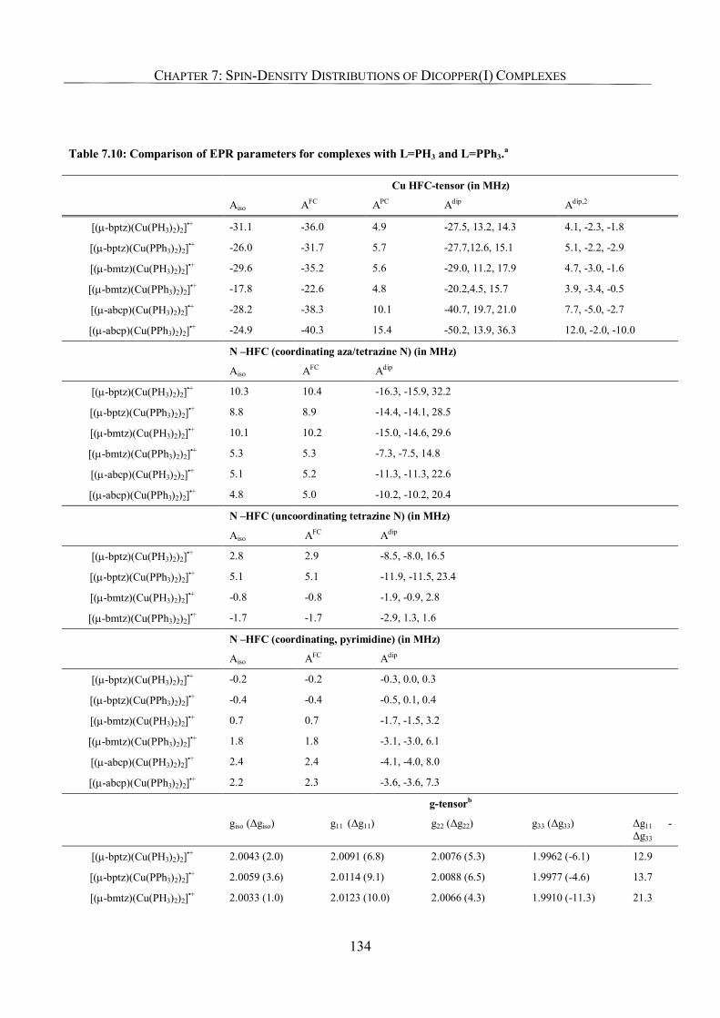
CHAPTER 7: SPIN-DENSITY DISTRIBUTIONS OF DICOPPER(I) COMPLEXES
134
Table 7.10: Comparison of EPR parameters for complexes with L=PH3 and L=PPh3.a
Cu HFC-tensor (in MHz)
Aiso AFC APC Adip Adip,2
[(µ-bptz)(Cu(PH3)2)2]•+ -31.1 -36.0 4.9 -27.5, 13.2, 14.3 4.1, -2.3, -1.8
[(µ-bptz)(Cu(PPh3)2)2]•+ -26.0 -31.7 5.7 -27.7,12.6, 15.1 5.1, -2.2, -2.9
[(µ-bmtz)(Cu(PH3)2)2]•+ -29.6 -35.2 5.6 -29.0, 11.2, 17.9 4.7, -3.0, -1.6
[(µ-bmtz)(Cu(PPh3)2)2]•+ -17.8 -22.6 4.8 -20.2,4.5, 15.7 3.9, -3.4, -0.5
[(µ-abcp)(Cu(PH3)2)2]•+ -28.2 -38.3 10.1 -40.7, 19.7, 21.0 7.7, -5.0, -2.7
[(µ-abcp)(Cu(PPh3)2)2]•+ -24.9 -40.3 15.4 -50.2, 13.9, 36.3 12.0, -2.0, -10.0
N –HFC (coordinating aza/tetrazine N) (in MHz)
Aiso AFC Adip
[(µ-bptz)(Cu(PH3)2)2]•+ 10.3 10.4 -16.3, -15.9, 32.2
[(µ-bptz)(Cu(PPh3)2)2]•+ 8.8 8.9 -14.4, -14.1, 28.5
[(µ-bmtz)(Cu(PH3)2)2]•+ 10.1 10.2 -15.0, -14.6, 29.6
[(µ-bmtz)(Cu(PPh3)2)2]•+ 5.3 5.3 -7.3, -7.5, 14.8
[(µ-abcp)(Cu(PH3)2)2]•+ 5.1 5.2 -11.3, -11.3, 22.6
[(µ-abcp)(Cu(PPh3)2)2]•+ 4.8 5.0 -10.2, -10.2, 20.4
N –HFC (uncoordinating tetrazine N) (in MHz)
Aiso AFC Adip
[(µ-bptz)(Cu(PH3)2)2]•+ 2.8 2.9 -8.5, -8.0, 16.5
[(µ-bptz)(Cu(PPh3)2)2]•+ 5.1 5.1 -11.9, -11.5, 23.4
[(µ-bmtz)(Cu(PH3)2)2]•+ -0.8 -0.8 -1.9, -0.9, 2.8
[(µ-bmtz)(Cu(PPh3)2)2]•+ -1.7 -1.7 -2.9, 1.3, 1.6
N –HFC (coordinating, pyrimidine) (in MHz)
Aiso AFC Adip
[(µ-bptz)(Cu(PH3)2)2]•+ -0.2 -0.2 -0.3, 0.0, 0.3
[(µ-bptz)(Cu(PPh3)2)2]•+ -0.4 -0.4 -0.5, 0.1, 0.4
[(µ-bmtz)(Cu(PH3)2)2]•+ 0.7 0.7 -1.7, -1.5, 3.2
[(µ-bmtz)(Cu(PPh3)2)2]•+ 1.8 1.8 -3.1, -3.0, 6.1
[(µ-abcp)(Cu(PH3)2)2]•+ 2.4 2.4 -4.1, -4.0, 8.0
[(µ-abcp)(Cu(PPh3)2)2]•+ 2.2 2.3 -3.6, -3.6, 7.3
g-tensorb
giso (Δgiso) g11 (Δg11) g22 (Δg22) g33 (Δg33) Δg11 - Δg33
[(µ-bptz)(Cu(PH3)2)2]•+ 2.0043 (2.0) 2.0091 (6.8) 2.0076 (5.3) 1.9962 (-6.1) 12.9
[(µ-bptz)(Cu(PPh3)2)2]•+ 2.0059 (3.6) 2.0114 (9.1) 2.0088 (6.5) 1.9977 (-4.6) 13.7
[(µ-bmtz)(Cu(PH3)2)2]•+ 2.0033 (1.0) 2.0123 (10.0) 2.0066 (4.3) 1.9910 (-11.3) 21.3
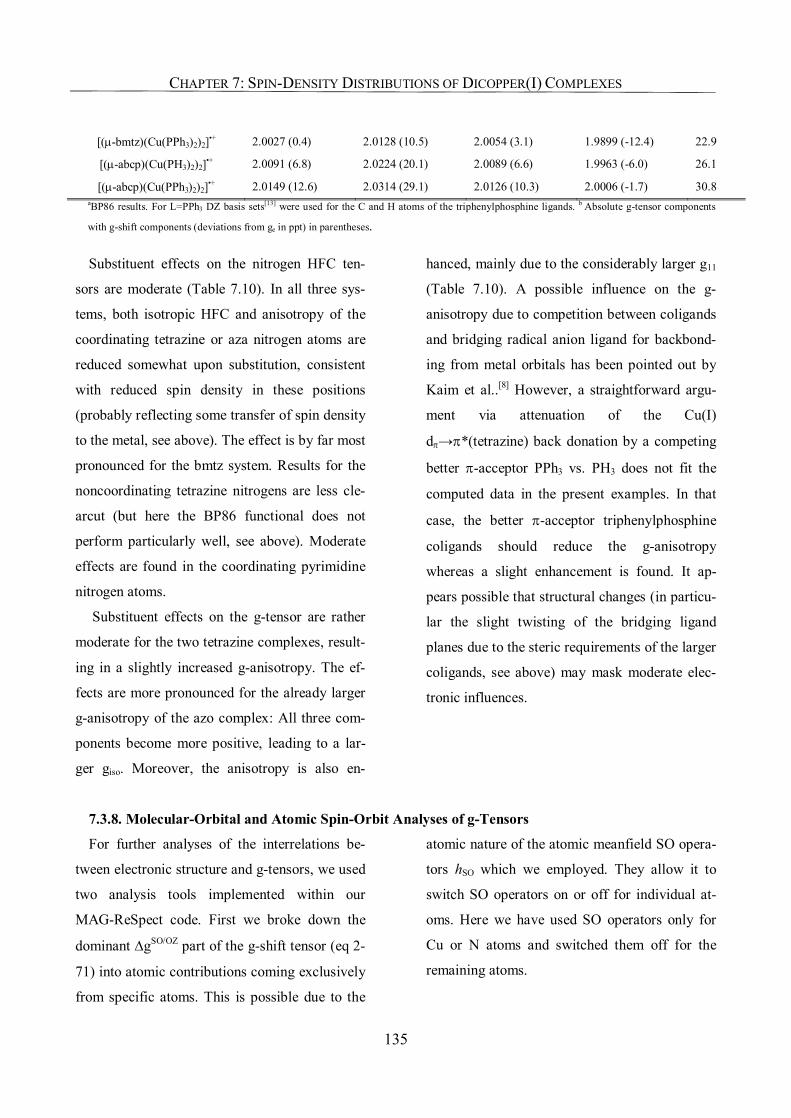
CHAPTER 7: SPIN-DENSITY DISTRIBUTIONS OF DICOPPER(I) COMPLEXES
135
[(µ-bmtz)(Cu(PPh3)2)2]•+ 2.0027 (0.4) 2.0128 (10.5) 2.0054 (3.1) 1.9899 (-12.4) 22.9
[(µ-abcp)(Cu(PH3)2)2]•+ 2.0091 (6.8) 2.0224 (20.1) 2.0089 (6.6) 1.9963 (-6.0) 26.1
[(µ-abcp)(Cu(PPh3)2)2]•+ 2.0149 (12.6) 2.0314 (29.1) 2.0126 (10.3) 2.0006 (-1.7) 30.8 aBP86 results. For L=PPh3 DZ basis sets[13] were used for the C and H atoms of the triphenylphosphine ligands. b Absolute g-tensor components
with g-shift components (deviations from ge in ppt) in parentheses.
Substituent effects on the nitrogen HFC ten-
sors are moderate (Table 7.10). In all three sys-
tems, both isotropic HFC and anisotropy of the
coordinating tetrazine or aza nitrogen atoms are
reduced somewhat upon substitution, consistent
with reduced spin density in these positions
(probably reflecting some transfer of spin density
to the metal, see above). The effect is by far most
pronounced for the bmtz system. Results for the
noncoordinating tetrazine nitrogens are less cle-
arcut (but here the BP86 functional does not
perform particularly well, see above). Moderate
effects are found in the coordinating pyrimidine
nitrogen atoms.
Substituent effects on the g-tensor are rather
moderate for the two tetrazine complexes, result-
ing in a slightly increased g-anisotropy. The ef-
fects are more pronounced for the already larger
g-anisotropy of the azo complex: All three com-
ponents become more positive, leading to a lar-
ger giso. Moreover, the anisotropy is also en-
hanced, mainly due to the considerably larger g11
(Table 7.10). A possible influence on the g-
anisotropy due to competition between coligands
and bridging radical anion ligand for backbond-
ing from metal orbitals has been pointed out by
Kaim et al..[8] However, a straightforward argu-
ment via attenuation of the Cu(I)
dπ→π*(tetrazine) back donation by a competing
better π-acceptor PPh3 vs. PH3 does not fit the
computed data in the present examples. In that
case, the better π-acceptor triphenylphosphine
coligands should reduce the g-anisotropy
whereas a slight enhancement is found. It ap-
pears possible that structural changes (in particu-
lar the slight twisting of the bridging ligand
planes due to the steric requirements of the larger
coligands, see above) may mask moderate elec-
tronic influences.
7.3.8. Molecular-Orbital and Atomic Spin-Orbit Analyses of g-Tensors
For further analyses of the interrelations be-
tween electronic structure and g-tensors, we used
two analysis tools implemented within our
MAG-ReSpect code. First we broke down the
dominant ∆gSO/OZ part of the g-shift tensor (eq 2-
71) into atomic contributions coming exclusively
from specific atoms. This is possible due to the
atomic nature of the atomic meanfield SO opera-
tors hSO which we employed. They allow it to
switch SO operators on or off for individual at-
oms. Here we have used SO operators only for
Cu or N atoms and switched them off for the
remaining atoms.
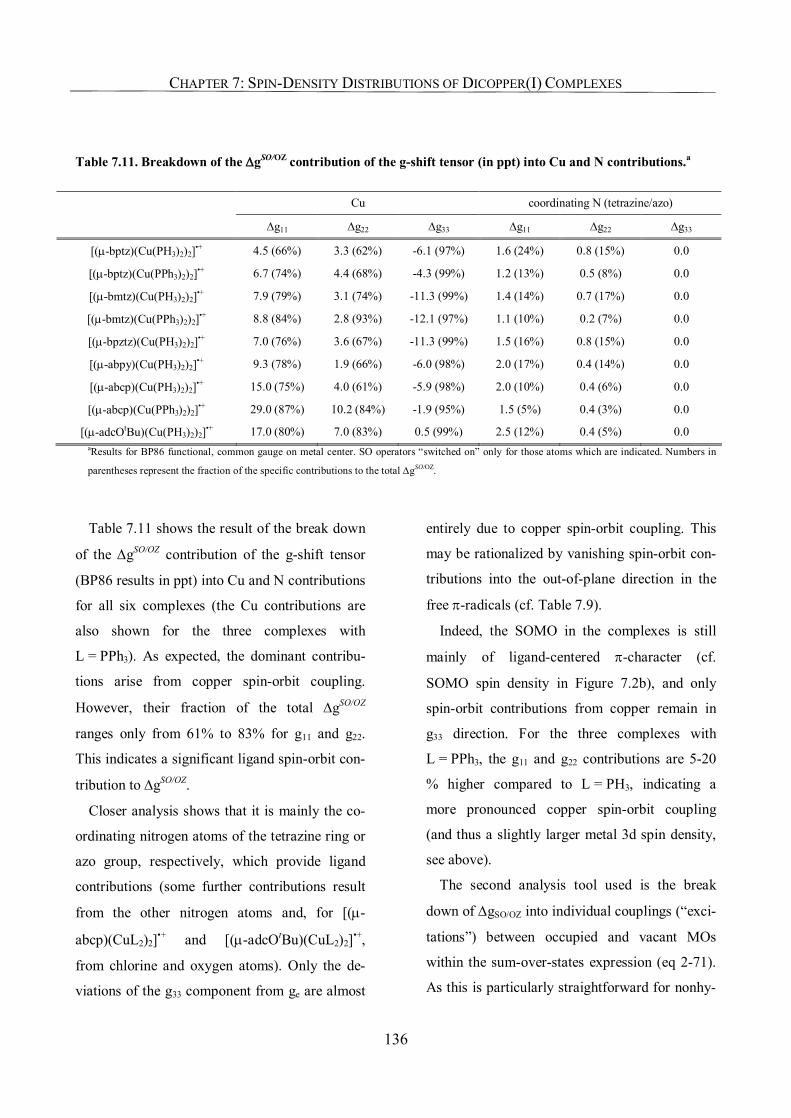
CHAPTER 7: SPIN-DENSITY DISTRIBUTIONS OF DICOPPER(I) COMPLEXES
136
Table 7.11. Breakdown of the ∆gSO/OZ contribution of the g-shift tensor (in ppt) into Cu and N contributions.a
Cu coordinating N (tetrazine/azo)
∆g11 ∆g22 ∆g33 ∆g11 ∆g22 ∆g33
[(µ-bptz)(Cu(PH3)2)2]•+ 4.5 (66%) 3.3 (62%) -6.1 (97%) 1.6 (24%) 0.8 (15%) 0.0
[(µ-bptz)(Cu(PPh3)2)2]•+ 6.7 (74%) 4.4 (68%) -4.3 (99%) 1.2 (13%) 0.5 (8%) 0.0
[(µ-bmtz)(Cu(PH3)2)2]•+ 7.9 (79%) 3.1 (74%) -11.3 (99%) 1.4 (14%) 0.7 (17%) 0.0
[(µ-bmtz)(Cu(PPh3)2)2]•+ 8.8 (84%) 2.8 (93%) -12.1 (97%) 1.1 (10%) 0.2 (7%) 0.0
[(µ-bpztz)(Cu(PH3)2)2]•+ 7.0 (76%) 3.6 (67%) -11.3 (99%) 1.5 (16%) 0.8 (15%) 0.0
[(µ-abpy)(Cu(PH3)2)2]•+ 9.3 (78%) 1.9 (66%) -6.0 (98%) 2.0 (17%) 0.4 (14%) 0.0
[(µ-abcp)(Cu(PH3)2)2]•+ 15.0 (75%) 4.0 (61%) -5.9 (98%) 2.0 (10%) 0.4 (6%) 0.0
[(µ-abcp)(Cu(PPh3)2)2]•+ 29.0 (87%) 10.2 (84%) -1.9 (95%) 1.5 (5%) 0.4 (3%) 0.0
[(µ-adcOtBu)(Cu(PH3)2)2]•+ 17.0 (80%) 7.0 (83%) 0.5 (99%) 2.5 (12%) 0.4 (5%) 0.0 aResults for BP86 functional, common gauge on metal center. SO operators “switched on” only for those atoms which are indicated. Numbers in
parentheses represent the fraction of the specific contributions to the total ∆gSO/OZ.
Table 7.11 shows the result of the break down
of the ∆gSO/OZ contribution of the g-shift tensor
(BP86 results in ppt) into Cu and N contributions
for all six complexes (the Cu contributions are
also shown for the three complexes with
L = PPh3). As expected, the dominant contribu-
tions arise from copper spin-orbit coupling.
However, their fraction of the total ∆gSO/OZ
ranges only from 61% to 83% for g11 and g22.
This indicates a significant ligand spin-orbit con-
tribution to ∆gSO/OZ.
Closer analysis shows that it is mainly the co-
ordinating nitrogen atoms of the tetrazine ring or
azo group, respectively, which provide ligand
contributions (some further contributions result
from the other nitrogen atoms and, for [(µ-
abcp)(CuL2)2]•+ and [(µ-adcOtBu)(CuL2)2]•+,
from chlorine and oxygen atoms). Only the de-
viations of the g33 component from ge are almost
entirely due to copper spin-orbit coupling. This
may be rationalized by vanishing spin-orbit con-
tributions into the out-of-plane direction in the
free π-radicals (cf. Table 7.9).
Indeed, the SOMO in the complexes is still
mainly of ligand-centered π-character (cf.
SOMO spin density in Figure 7.2b), and only
spin-orbit contributions from copper remain in
g33 direction. For the three complexes with
L = PPh3, the g11 and g22 contributions are 5-20
% higher compared to L = PH3, indicating a
more pronounced copper spin-orbit coupling
(and thus a slightly larger metal 3d spin density,
see above).
The second analysis tool used is the break
down of ∆gSO/OZ into individual couplings (“exci-
tations”) between occupied and vacant MOs
within the sum-over-states expression (eq 2-71).
As this is particularly straightforward for nonhy-
CHAPTER 7: SPIN-DENSITY DISTRIBUTIONS OF DICOPPER(I) COMPLEXES
137
brid functionals, where the equations are not
coupled by HF exchange terms, we refer in the
following to BP86 results.
The analyses show excitations from doubly
occupied MOs with β-spin to the β-component of
the SOMO to dominate the g-tensor for the azo
complexes (between +14 ppt and +27 ppt for the
largest component ∆g11). The corresponding
excitations contribute less (between +5 ppt and
+8 ppt) for the tetrazine complexes. This reflects
the larger metal character of these doubly occu-
pied MOs for the azo systems, connected to their
more pronounced π-acceptor ability. Excitations
from SOMO to virtual MOs (with α-spin) con-
tribute negatively to g11, between -4 ppt and -
9 ppt for both azo and tetrazine ligands. The
relatively large positive Δg11 for the azo com-
plexes and the small Δg11 values for the tetrazine
systems result.
For ∆g22 and ∆g33 the interplay between the
different kinds of excitations is more subtle and
may be analyzed only incompletely. Negative
Δg33 values arise partly from SOMO-virtual exci-
tations. This agrees with the usual expectation
that α-α couplings should contribute negatively
to ∆gSO/OZ.
However, except for [(µ-adcOtBu)(CuL2)2]•+,
where β-β couplings from doubly occupied MOs
to SOMO contribute positively to all three tensor
components, these couplings make an additional
negative contribution to Δg33. This suggests that
the spin-orbit and orbital-Zeeman matrix ele-
ments may have opposite sign (cf. eq. 2-71),
which usually reflects strongly off-center ring
currents.
Obviously, the electronic situation in these
ligand centered complexes does not suit itself
very well for a particularly simple interpretation
of the g-tensor. However, one sees clearly the
stronger π-interactions between metal and bridg-
ing ligand for the azo compared to the tetrazine
complexes, as reflected in the more positive Δg11
tensor components. The computationally some-
what more negative Δg33 for the tetrazine com-
plexes reflects mainly a slightly larger role of
SOMO-virtual excitations.
7.4. Conclusions
The study of these dinuclear copper complexes
with bridging radical-anion ligands has provided
us with more insight into the interrelations be-
tween electronic structure, spin density, and EPR
parameters for this intriguing bonding situation
than hitherto available. In particular, the ability
of state-of-the art density functionals to describe
metal and ligand hyperfine couplings and elec-
tronic g-tensors well (although no “best” func-
tional is easily identified), allowed more detailed
analyses than was possible for a previously stud-
ied test set of dinuclear rhenium complexes.[3]
The unexpected dependence of the isotropic
metal hyperfine couplings on exchange-
correlation functional has drawn our attention to
a subtle spin polarization of the σ-framework of
the bridging ligand by the π-type SOMO. In
analogy to the better-known McConnell mecha-
CHAPTER 7: SPIN-DENSITY DISTRIBUTIONS OF DICOPPER(I) COMPLEXES
138
nism in organic π-radicals, this spin polarization
transfers some negative spin density into the
copper 4s-orbitals and thereby changes the origin
of the negative isotropic metal hyperfine cou-
pling fundamentally compared to the currently
established picture of the mechanisms of transi-
tion-metal hyperfine couplings via core-shell
spin polarization.[15]
In spite of their clearly ligand-centered spin
density, the title complexes exhibit appreciable
electronic communication between the two metal
centers. This is reflected in the EPR parameters,
and it makes these types of “ligand-centered”
radical complexes attractive as components of
supermolecular functional materials.
139
Chapter 8
Bis(semiquinonato)copper Complexes –
Change of Spin State by Twisting the Ring System
8.1. Introduction
In this chapter we will again turn to complexes
with “noninnocent” ligands (see Chapter 6). We
will compare two copper complexes: (a) The
[(Qx•-)CuII(Qx
•-)] complex 1 where Qx•- is an
iminobenzosemiquinone ligand with an benzene
substituent at the imine, as described by Chaud-
huri et. al.[1], and (b) the [(Qx•-)CuII(Qx
•-)] com-
plex 2, where an additional SMe sidechain in the
benzene substituent of the imine is present. The
latter complex was synthesized and characterised
by Ye et al.[2].
While the two compounds are very similar in
composition, they nevertheless exhibit a signifi-
cant difference in geometry and also a com-
pletely different electronic structure. 1 is a
[(Qx•-)CuII(Qx
•-)] complex with planar configura-
tion and has a (↑↑↓) ground state where the two
benzosemiquinone radical ligands are antiferro-
magnetically coupled.
In contrast, in 2 the two ring systems are
twisted, and the spin ground state should rather
be described as a (↑↓↑) situation with dominating
antiferromagnetic couplings between the metal
and the ligands. The geometrical structure of the
two compounds is shown in Figure 8.1.
The observation of two completely different
spin states of copper complexes connected to a
geometrical change is highly relevant because
tetracoordinate CuII centers in a non-planar envi-
ronment are often found in connection with cop-
per enzyme modeling or in the copper centers of
blue-copper proteins (cf. Chapter 5). Such cen-
ters act as electron transfer sites and switch usu-
ally between CuII and CuI states. In the case
when one noninnocent ligands is present the
valence tautomer equilibrium CuII(Q2-)
CuI(Q•-) is known for oxidase enzymes.[3][4]
However, the situation becomes even more inter-
esting if several noninnocent quinone ligands are
involved due to the fascinating spin-spin interac-
tions in such stable three spin-systems.[1][5]
Quantum-chemical calculations provide a
good way to examine the spin state of these
complexes in detail. For the two bis(semiquino-
nato)copper complexes described above one
would intuitively suggest that the change in elec-
tronic structure is due to the different structure
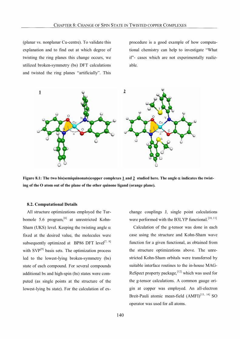
CHAPTER 8: CHANGE OF SPIN STATE IN TWISTED COPPER COMPLEXES
140
(planar vs. nonplanar Cu-centre). To validate this
explanation and to find out at which degree of
twisting the ring planes this change occurs, we
utilized broken-symmetry (bs) DFT calculations
and twisted the ring planes “artificially”. This
procedure is a good example of how computa-
tional chemistry can help to investigate “What
if”- cases which are not experimentally realiz-
able.
Figure 8.1: The two bis(semiquinonato)copper complexes 1 and 2 studied here. The angle α indicates the twist-
ing of the O atom out of the plane of the other quinone ligand (orange plane).
8.2. Computational Details
All structure optimizations employed the Tur-
bomole 5.6 program,[6] at unrestricted Kohn-
Sham (UKS) level. Keeping the twisting angle α
fixed at the desired value, the molecules were
subsequently optimized at BP86 DFT level[7, 8]
with SVP[9] basis sets. The optimization process
led to the lowest-lying broken-symmetry (bs)
state of each compound. For several compounds
additional bs and high-spin (hs) states were com-
puted (as single points at the structure of the
lowest-lying bs state). For the calculation of ex-
change couplings J, single point calculations
were performed with the B3LYP functional.[10, 11]
Calculation of the g-tensor was done in each
case using the structure and Kohn-Sham wave
function for a given functional, as obtained from
the structure optimizations above. The unre-
stricted Kohn-Sham orbitals were transferred by
suitable interface routines to the in-house MAG-
ReSpect property package,[12] which was used for
the g-tensor calculations. A common gauge ori-
gin at copper was employed. An all-electron
Breit-Pauli atomic mean-field (AMFI)[13, 14] SO
operator was used for all atoms.
CHAPTER 8: CHANGE OF SPIN STATE IN TWISTED COPPER COMPLEXES
141
The exchange coupling constants were calcu-
lated according to the methodology introduced in
chapter 2, applying a similar procedure as de-
scribed in ref. [15]. Molecular structures, canoni-
cal and natural orbitals, and spin-density isosur-
faces are displayed with the Molekel 4.3 pro-
gram.[16]
8.3. Results and Discussion
8.3.1. The g-Tensor as a Probe of the Electronic Structure
In Tables 8.1 and 8.2 the calculated values
(BP86 results) for the g-tensors of compound 1
and 2 are shown. However, there is a critical
difference to the g-tensors which were calculated
in this thesis so far: the present g-tensors are
calculated for a bs state and therefore do not
represent g-tensors of “real” spin states. Note
that these g-tensors – with calculated values for
the lowest lying bs state – suffer from spin con-
tamination. <S2> values are given in Tables 8.1
and 8.2. The deviation from the spin expectation
value <S2> = 0.75 for a pure doublet state could
be regarded as an indication how large the ad-
mixture of the hs-state to the electronic ground
state is.[17]
Nevertheless the g-tensor even of the spin con-
taminated bs states expresses the main difference
between the two electronic states which were
experimentally observed: on the one hand g val-
ues which provide the typical features of a CuII
complex, on the other hand g values which are
found for semiquinone radical anions coordi-
nated to copper[4]. We therefore conclude that the
calculated bs state, although spin contaminated,
describes sufficiently the electronic features. We
will thus start our discussion with a comparison
of calculated and experimental g values for com-
pounds 1 and 2 at their X-ray structures.
Especially the calculated g11 and g22 compo-
nents are in surprisingly good accordance with
the experimentally determined values. In con-
trast, there are deficiencies in the description of
the g33 components, where the calculated values
are noticeably smaller than the experimental
ones. The use of a higher amount of HF ex-
change which is usually a good way to improve
g-tensor results (see previous chapters) increases
the spin contamination drastically (up to
<S2>=1.8) and does help only partly: in com-
pound 1 g33 is indeed increased to 2.1332 where-
as in 2 g33 is further decreased to a value of
1.9654. This behavior is due to the fact that in
the former case the description of a metal-
centered radical becomes even more metal cen-
tered with a larger amount of HF exchange. On
the other hand a ligand-centered radical also
tends to be more ligand-centered when the
amount of HF exchange is increased (see Chap-
ter 7). In contrast the character of the hs state is
always predominantly a metal-centered CuII
situation. Admixture of the hs state into the bs
state should therefore enhance the CuII radical
character and maybe increase the g33 component.
For 1 this admixture would amplify the situation
which is already present whereas for 2 this ad-
mixture would push the radical character in an
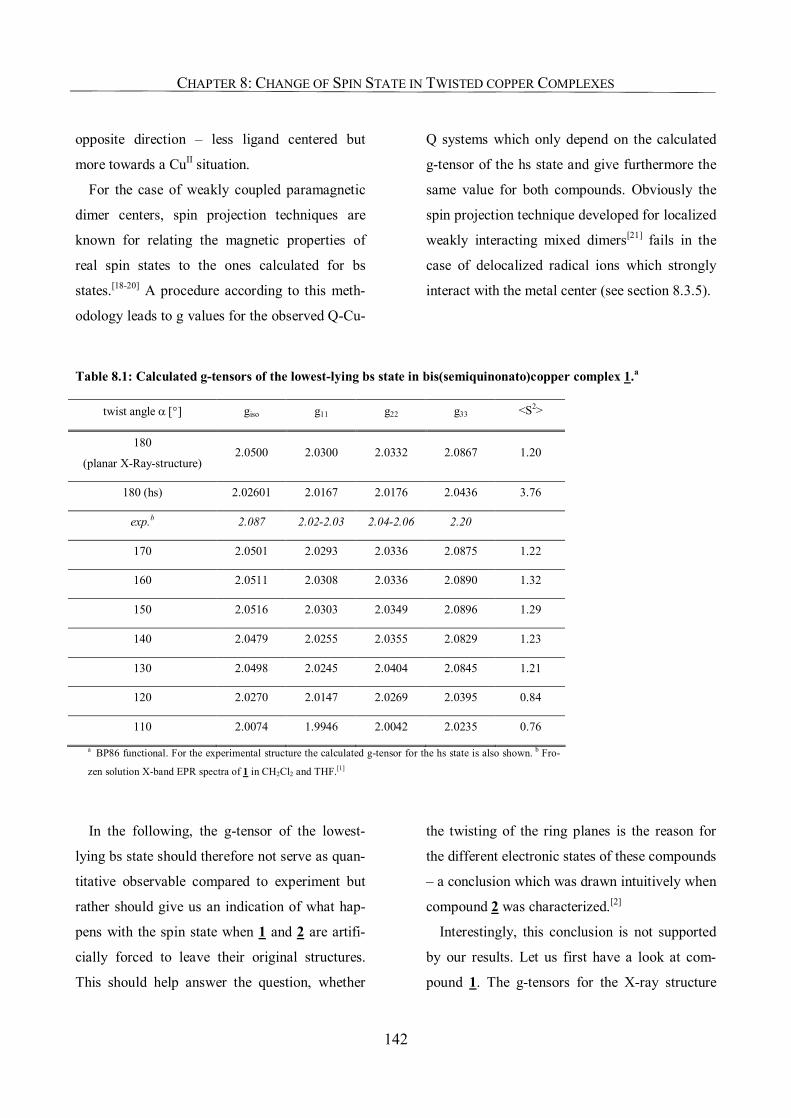
CHAPTER 8: CHANGE OF SPIN STATE IN TWISTED COPPER COMPLEXES
142
opposite direction – less ligand centered but
more towards a CuII situation.
For the case of weakly coupled paramagnetic
dimer centers, spin projection techniques are
known for relating the magnetic properties of
real spin states to the ones calculated for bs
states.[18-20] A procedure according to this meth-
odology leads to g values for the observed Q-Cu-
Q systems which only depend on the calculated
g-tensor of the hs state and give furthermore the
same value for both compounds. Obviously the
spin projection technique developed for localized
weakly interacting mixed dimers[21] fails in the
case of delocalized radical ions which strongly
interact with the metal center (see section 8.3.5).
Table 8.1: Calculated g-tensors of the lowest-lying bs state in bis(semiquinonato)copper complex 1.a
twist angle α [°] giso g11 g22 g33 <S2>
180
(planar X-Ray-structure) 2.0500 2.0300 2.0332 2.0867 1.20
180 (hs) 2.02601 2.0167 2.0176 2.0436 3.76
exp.b 2.087 2.02-2.03 2.04-2.06 2.20
170 2.0501 2.0293 2.0336 2.0875 1.22
160 2.0511 2.0308 2.0336 2.0890 1.32
150 2.0516 2.0303 2.0349 2.0896 1.29
140 2.0479 2.0255 2.0355 2.0829 1.23
130 2.0498 2.0245 2.0404 2.0845 1.21
120 2.0270 2.0147 2.0269 2.0395 0.84
110 2.0074 1.9946 2.0042 2.0235 0.76
a BP86 functional. For the experimental structure the calculated g-tensor for the hs state is also shown. b Fro-
zen solution X-band EPR spectra of 1 in CH2Cl2 and THF.[1]
In the following, the g-tensor of the lowest-
lying bs state should therefore not serve as quan-
titative observable compared to experiment but
rather should give us an indication of what hap-
pens with the spin state when 1 and 2 are artifi-
cially forced to leave their original structures.
This should help answer the question, whether
the twisting of the ring planes is the reason for
the different electronic states of these compounds
– a conclusion which was drawn intuitively when
compound 2 was characterized.[2]
Interestingly, this conclusion is not supported
by our results. Let us first have a look at com-
pound 1. The g-tensors for the X-ray structure
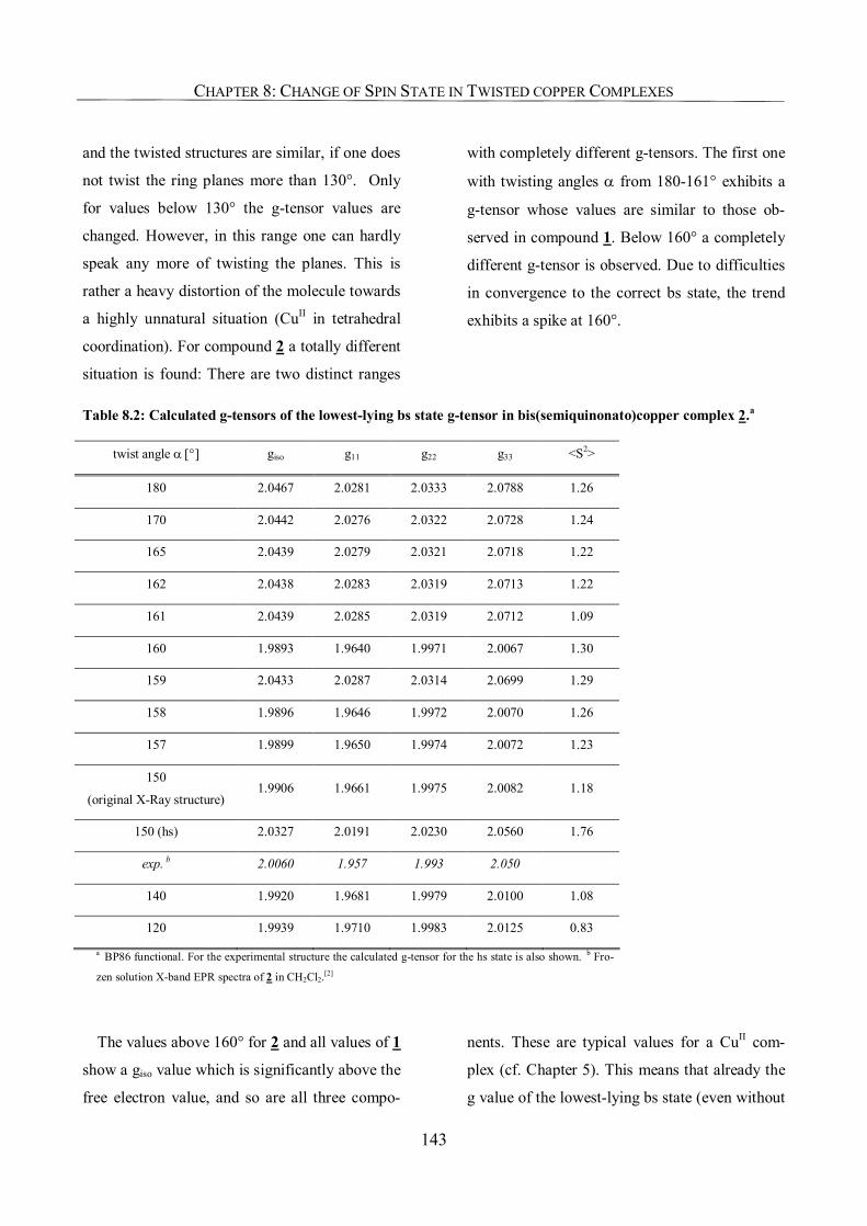
CHAPTER 8: CHANGE OF SPIN STATE IN TWISTED COPPER COMPLEXES
143
and the twisted structures are similar, if one does
not twist the ring planes more than 130°. Only
for values below 130° the g-tensor values are
changed. However, in this range one can hardly
speak any more of twisting the planes. This is
rather a heavy distortion of the molecule towards
a highly unnatural situation (CuII in tetrahedral
coordination). For compound 2 a totally different
situation is found: There are two distinct ranges
with completely different g-tensors. The first one
with twisting angles α from 180-161° exhibits a
g-tensor whose values are similar to those ob-
served in compound 1. Below 160° a completely
different g-tensor is observed. Due to difficulties
in convergence to the correct bs state, the trend
exhibits a spike at 160°.
Table 8.2: Calculated g-tensors of the lowest-lying bs state g-tensor in bis(semiquinonato)copper complex 2.a
twist angle α [°] giso g11 g22 g33 <S2>
180 2.0467 2.0281 2.0333 2.0788 1.26
170 2.0442 2.0276 2.0322 2.0728 1.24
165 2.0439 2.0279 2.0321 2.0718 1.22
162 2.0438 2.0283 2.0319 2.0713 1.22
161 2.0439 2.0285 2.0319 2.0712 1.09
160 1.9893 1.9640 1.9971 2.0067 1.30
159 2.0433 2.0287 2.0314 2.0699 1.29
158 1.9896 1.9646 1.9972 2.0070 1.26
157 1.9899 1.9650 1.9974 2.0072 1.23
150
(original X-Ray structure) 1.9906 1.9661 1.9975 2.0082 1.18
150 (hs) 2.0327 2.0191 2.0230 2.0560 1.76
exp. b 2.0060 1.957 1.993 2.050
140 1.9920 1.9681 1.9979 2.0100 1.08
120 1.9939 1.9710 1.9983 2.0125 0.83
a BP86 functional. For the experimental structure the calculated g-tensor for the hs state is also shown. b Fro-
zen solution X-band EPR spectra of 2 in CH2Cl2.[2]
The values above 160° for 2 and all values of 1
show a giso value which is significantly above the
free electron value, and so are all three compo-
nents. These are typical values for a CuII com-
plex (cf. Chapter 5). This means that already the
g value of the lowest-lying bs state (even without
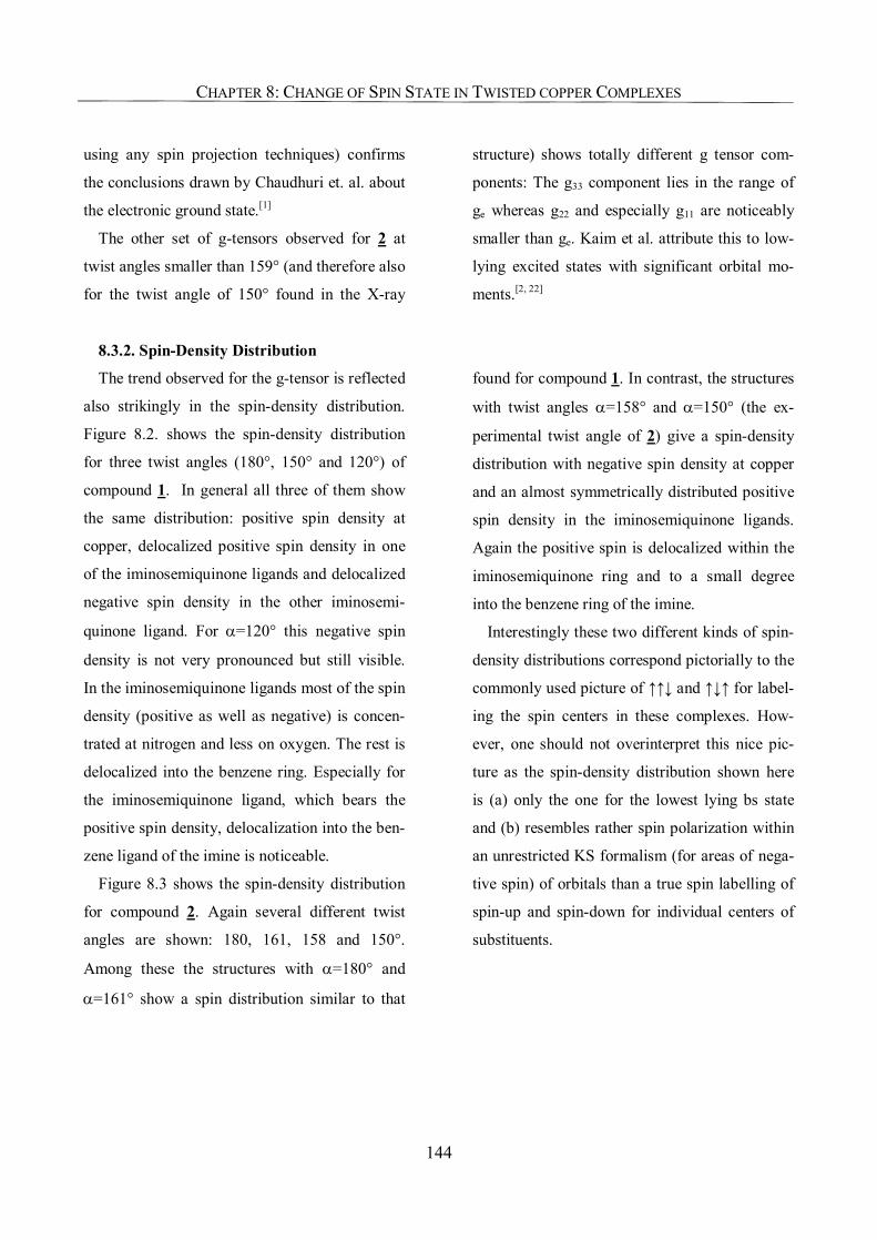
CHAPTER 8: CHANGE OF SPIN STATE IN TWISTED COPPER COMPLEXES
144
using any spin projection techniques) confirms
the conclusions drawn by Chaudhuri et. al. about
the electronic ground state.[1]
The other set of g-tensors observed for 2 at
twist angles smaller than 159° (and therefore also
for the twist angle of 150° found in the X-ray
structure) shows totally different g tensor com-
ponents: The g33 component lies in the range of
ge whereas g22 and especially g11 are noticeably
smaller than ge. Kaim et al. attribute this to low-
lying excited states with significant orbital mo-
ments.[2, 22]
8.3.2. Spin-Density Distribution
The trend observed for the g-tensor is reflected
also strikingly in the spin-density distribution.
Figure 8.2. shows the spin-density distribution
for three twist angles (180°, 150° and 120°) of
compound 1. In general all three of them show
the same distribution: positive spin density at
copper, delocalized positive spin density in one
of the iminosemiquinone ligands and delocalized
negative spin density in the other iminosemi-
quinone ligand. For α=120° this negative spin
density is not very pronounced but still visible.
In the iminosemiquinone ligands most of the spin
density (positive as well as negative) is concen-
trated at nitrogen and less on oxygen. The rest is
delocalized into the benzene ring. Especially for
the iminosemiquinone ligand, which bears the
positive spin density, delocalization into the ben-
zene ligand of the imine is noticeable.
Figure 8.3 shows the spin-density distribution
for compound 2. Again several different twist
angles are shown: 180, 161, 158 and 150°.
Among these the structures with α=180° and
α=161° show a spin distribution similar to that
found for compound 1. In contrast, the structures
with twist angles α=158° and α=150° (the ex-
perimental twist angle of 2) give a spin-density
distribution with negative spin density at copper
and an almost symmetrically distributed positive
spin density in the iminosemiquinone ligands.
Again the positive spin is delocalized within the
iminosemiquinone ring and to a small degree
into the benzene ring of the imine.
Interestingly these two different kinds of spin-
density distributions correspond pictorially to the
commonly used picture of ↑↑↓ and ↑↓↑ for label-
ing the spin centers in these complexes. How-
ever, one should not overinterpret this nice pic-
ture as the spin-density distribution shown here
is (a) only the one for the lowest lying bs state
and (b) resembles rather spin polarization within
an unrestricted KS formalism (for areas of nega-
tive spin) of orbitals than a true spin labelling of
spin-up and spin-down for individual centers of
substituents.
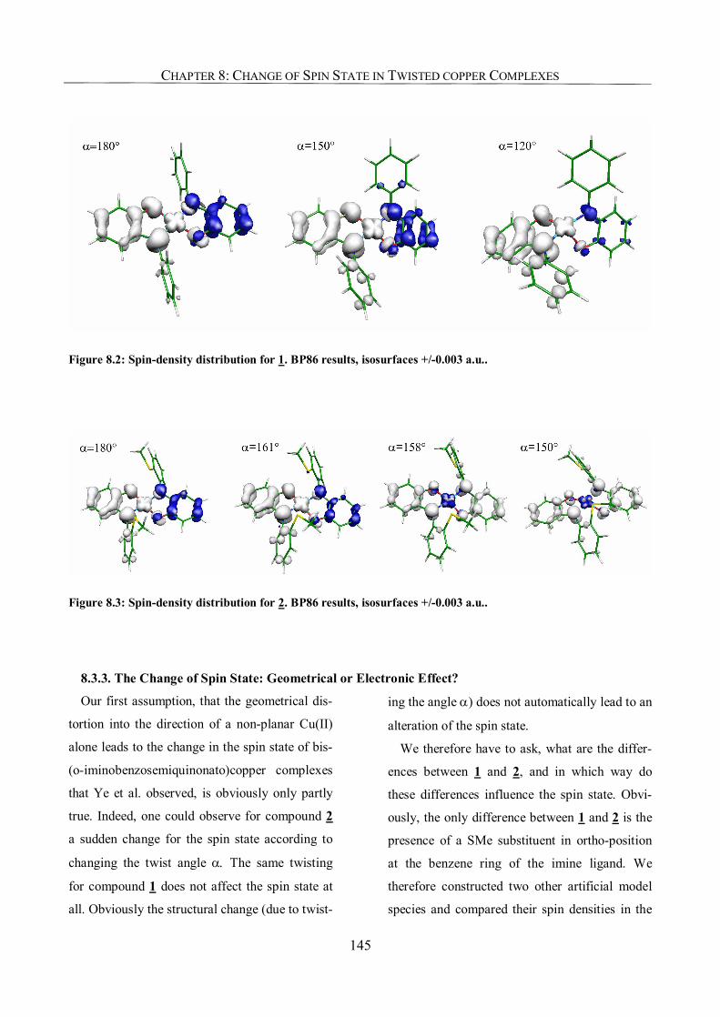
CHAPTER 8: CHANGE OF SPIN STATE IN TWISTED COPPER COMPLEXES
145
Figure 8.2: Spin-density distribution for 1. BP86 results, isosurfaces +/-0.003 a.u..
Figure 8.3: Spin-density distribution for 2. BP86 results, isosurfaces +/-0.003 a.u..
8.3.3. The Change of Spin State: Geometrical or Electronic Effect?
Our first assumption, that the geometrical dis-
tortion into the direction of a non-planar Cu(II)
alone leads to the change in the spin state of bis-
(o-iminobenzosemiquinonato)copper complexes
that Ye et al. observed, is obviously only partly
true. Indeed, one could observe for compound 2
a sudden change for the spin state according to
changing the twist angle α. The same twisting
for compound 1 does not affect the spin state at
all. Obviously the structural change (due to twist-
ing the angle α) does not automatically lead to an
alteration of the spin state.
We therefore have to ask, what are the differ-
ences between 1 and 2, and in which way do
these differences influence the spin state. Obvi-
ously, the only difference between 1 and 2 is the
presence of a SMe substituent in ortho-position
at the benzene ring of the imine ligand. We
therefore constructed two other artificial model
species and compared their spin densities in the
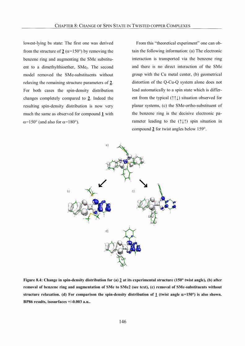
CHAPTER 8: CHANGE OF SPIN STATE IN TWISTED COPPER COMPLEXES
146
lowest-lying bs state: The first one was derived
from the structure of 2 (α=150°) by removing the
benzene ring and augmenting the SMe substitu-
ent to a dimethylthioether, SMe2. The second
model removed the SMe-substituents without
relaxing the remaining structure parameters of 2.
For both cases the spin-density distribution
changes completely compared to 2. Indeed the
resulting spin-density distribution is now very
much the same as observed for compound 1 with
α=150° (and also for α=180°).
From this “theoretical experiment” one can ob-
tain the following information: (a) The electronic
interaction is transported via the benzene ring
and there is no direct interaction of the SMe
group with the Cu metal center, (b) geometrical
distortion of the Q-Cu-Q system alone does not
lead automatically to a spin state which is differ-
ent from the typical (↑↑↓) situation observed for
planar systems, (c) the SMe-ortho-substituent of
the benzene ring is the decisive electronic pa-
rameter leading to the (↑↓↑) spin situation in
compound 2 for twist angles below 159°.
Figure 8.4: Change in spin-density distribution for (a) 2 at its experimental structure (150° twist angle), (b) after
removal of benzene ring and augmentation of SMe to SMe2 (see text), (c) removal of SMe-substituents without
structure relaxation. (d) For comparison the spin-density distribution of 1 (twist angle α=150°) is also shown.
BP86 results, isosurfaces +/-0.003 a.u..
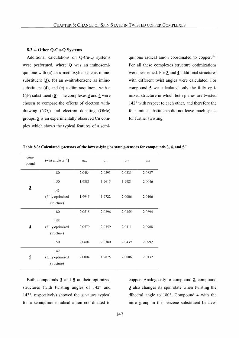
CHAPTER 8: CHANGE OF SPIN STATE IN TWISTED COPPER COMPLEXES
147
8.3.4. Other Q-Cu-Q Systems
Additional calculations on Q-Cu-Q systems
were performed, where Q was an iminosemi-
quinone with (a) an o-methoxybenzene as imine-
substituent (3), (b) an o-nitrobenzene as imine-
substituent (4), and (c) a diiminoquinone with a
C6F5 substituent (5). The complexes 3 and 4 were
chosen to compare the effects of electron with-
drawing (NO2) and electron donating (OMe)
groups. 5 is an experimentally observed Cu com-
plex which shows the typical features of a semi-
quinone radical anion coordinated to copper.[23]
For all these complexes structure optimizations
were performed. For 3 and 4 additional structures
with different twist angles were calculated. For
compound 5 we calculated only the fully opti-
mized structure in which both planes are twisted
142° with respect to each other, and therefore the
four imine substituents did not leave much space
for further twisting.
Table 8.3: Calculated g-tensors of the lowest-lying bs state g-tensors for compounds 3, 4, and 5.a
com-
pound twist angle α [°] giso g11 g22 g33
180 2.0484 2.0293 2.0331 2.0827
150 1.9881 1.9615 1.9981 2.0046
3 143
(fully optimized
structure)
1.9945 1.9722 2.0006 2.0106
180 2.0515 2.0296 2.0355 2.0894
155
(fully optimized
structure)
2.0579 2.0359 2.0411 2.0968 4
150 2.0604 2.0380 2.0439 2.0992
5
142
(fully optimized
structure)
2.0004 1.9875 2.0006 2.0132
Both compounds 3 and 5 at their optimized
structures (with twisting angles of 142° and
143°, respectively) showed the g values typical
for a semiquinone radical anion coordinated to
copper. Analogously to compound 2, compound
3 also changes its spin state when twisting the
dihedral angle to 180°. Compound 4 with the
nitro group in the benzene substituent behaves
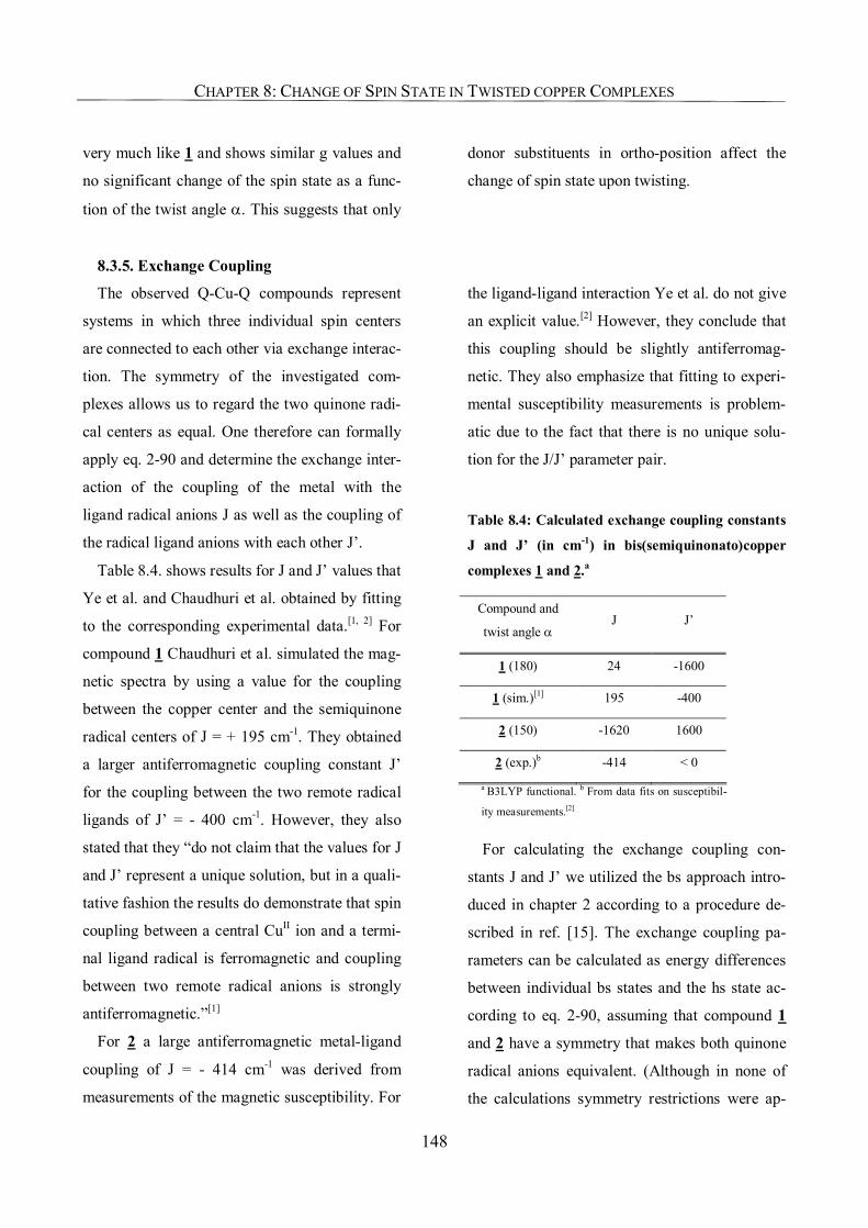
CHAPTER 8: CHANGE OF SPIN STATE IN TWISTED COPPER COMPLEXES
148
very much like 1 and shows similar g values and
no significant change of the spin state as a func-
tion of the twist angle α. This suggests that only
donor substituents in ortho-position affect the
change of spin state upon twisting.
8.3.5. Exchange Coupling
The observed Q-Cu-Q compounds represent
systems in which three individual spin centers
are connected to each other via exchange interac-
tion. The symmetry of the investigated com-
plexes allows us to regard the two quinone radi-
cal centers as equal. One therefore can formally
apply eq. 2-90 and determine the exchange inter-
action of the coupling of the metal with the
ligand radical anions J as well as the coupling of
the radical ligand anions with each other J’.
Table 8.4. shows results for J and J’ values that
Ye et al. and Chaudhuri et al. obtained by fitting
to the corresponding experimental data.[1, 2] For
compound 1 Chaudhuri et al. simulated the mag-
netic spectra by using a value for the coupling
between the copper center and the semiquinone
radical centers of J = + 195 cm-1. They obtained
a larger antiferromagnetic coupling constant J’
for the coupling between the two remote radical
ligands of J’ = - 400 cm-1. However, they also
stated that they “do not claim that the values for J
and J’ represent a unique solution, but in a quali-
tative fashion the results do demonstrate that spin
coupling between a central CuII ion and a termi-
nal ligand radical is ferromagnetic and coupling
between two remote radical anions is strongly
antiferromagnetic.”[1]
For 2 a large antiferromagnetic metal-ligand
coupling of J = - 414 cm-1 was derived from
measurements of the magnetic susceptibility. For
the ligand-ligand interaction Ye et al. do not give
an explicit value.[2] However, they conclude that
this coupling should be slightly antiferromag-
netic. They also emphasize that fitting to experi-
mental susceptibility measurements is problem-
atic due to the fact that there is no unique solu-
tion for the J/J’ parameter pair.
Table 8.4: Calculated exchange coupling constants
J and J’ (in cm-1) in bis(semiquinonato)copper
complexes 1 and 2.a
Compound and
twist angle α J J’
1 (180) 24 -1600
1 (sim.)[1] 195 -400
2 (150) -1620 1600
2 (exp.)b -414 < 0
a B3LYP functional. b From data fits on susceptibil-
ity measurements.[2]
For calculating the exchange coupling con-
stants J and J’ we utilized the bs approach intro-
duced in chapter 2 according to a procedure de-
scribed in ref. [15]. The exchange coupling pa-
rameters can be calculated as energy differences
between individual bs states and the hs state ac-
cording to eq. 2-90, assuming that compound 1
and 2 have a symmetry that makes both quinone
radical anions equivalent. (Although in none of
the calculations symmetry restrictions were ap-
CHAPTER 8: CHANGE OF SPIN STATE IN TWISTED COPPER COMPLEXES
149
plied, both compounds are roughly C2-
symmetrical and fulfill this condition). Calcula-
tions of the second-lowest bs state turned out to
be difficult with the BP86 functional. Therefore
we used the hybrid B3LYP functional which
ensured better convergence.
Table 8.4. shows the results of the calculated J
values (with the B3LYP functional) in compari-
son to the fitted data by Ye et al. and Chaudhuri
et al..
Our calculated values for compound 1 deviate
from the fitted values up to a factor of six. How-
ever, the J values are qualitatively consistent
with the observed electronic structure. They de-
scribe the interaction between the ligand spin
centers as strongly antiferromagnetic, whereas
the metal-ligand interaction is characterized by a
small ferromagnetic coupling. This small ferro-
magnetic coupling could be explained as a su-
perposition of the ferromagnetic coupling of the
metal radical to the ligand radical anion on the
one side and the simultaneous antiferromagnetic
coupling to the radical ligand on the other side
(as the spin labeling indicates). Obviously the
ferromagnetic coupling overcompensates the
antiferromagnetic coupling slightly so that an
overall small ferromagnetic coupling results.
In contrast, 2 shows a large antiferromagnetic
metal-ligand coupling in accordance with the
experimental assignment as a copper-coordinated
semiquinone radical anion. Again our calculated
J value is larger than the value determined by Ye
et al. from magnetic susceptibility data. For the
ligand-ligand interaction we found a large anti-
ferromagnetic coupling, consistent with a spin
labeling of (↑↓↑). Ye et al. claimed that this cou-
pling should be also slightly antiferromagnetic,
but they could not determine an explicit value
(see above).
Nevertheless, we should also keep in mind that
the way the J values were calculated present only
a crude estimate of the exchange interaction. In
fact, we have accepted several rough approxima-
tions. For instance the neglect of the delocalized
nature of the ligand radical ions was not consid-
ered (see Chapter 2).
8.4. Conclusions
To monitor the electronic state of these inter-
esting 3-spin species as a function of structure,
we used the g-tensors of the calculated bs states
as probe of spin state. Although the bs state is
highly spin contaminated it provides a surpris-
ingly good description of the experimentally
observed g values. Remaining shortcomings
could be explained by admixture of the hs state.
Contrary to our expectation the reason for the
different electronic states found in compounds 1
and 2 is not an automatic consequence of the
geometrical distortion, namely the twist of the
planes of the quinonoid radical ligands alone. It
is rather due to electronic substituent effects
connected with this twisting. This was demon-
strated by an “artificial” twisting of this angle
which revealed a change of spin state for com-
pound 2 when the twist angle is below 159°. In
contrast, no comparable behavior was found for
compound 1. Calculations on 2 with particular
CHAPTER 8: CHANGE OF SPIN STATE IN TWISTED COPPER COMPLEXES
150
parts cut out of the molecule, and additional cal-
culations on Q-Cu-Q systems with electron with-
drawing and electron donating groups, indicated
that indeed very subtle electronic effects are re-
sponsible for the differences in the spin state of
the observed Q-Cu-Q systems. Obviously only
electron-rich aromatic substituents like o-
substituted SMe- and OMe- iminobenzenes favor
the spin state with ferromagnetically coupled
radical ligands when the quinone planes are
twisted out of coplanarity.
The exchange coupling parameters J and J’
have been calculated for the X-ray structures of 1
and 2. Their accordance with fitted data for EPR
spectra or susceptibility measurements is only
modest. Nevertheless, since the experimental
data rely on several limiting boundary condi-
tions[1, 2], and since there are particular shortcom-
ings of the methodology for calculating exchange
coupling parameters for the title complexes, the
accuracy of these values should not be overem-
phasized. In any case they describe the exchange
interactions well from a qualitative point of view.
151
Bibliography
Introduction [1] F. Neese, in Calculation of NMR and EPR Parameters: Theory and Applications (Eds.: M, Kaupp, M. Bühl, V. G. Mal-
kin), pp 581-590, Wiley-VCH, Weinheim, 2004. [2] W. R. Hagen, Adv. Inorg. Chem. 1992, 38, 165. [3] B. Guigliarelli, P. Bertrand, Adv. Inorg. Chem. 1999, 47, 421. [4] E. I. Solomon, M. J. Baldwin, M. D. Lowery, Chem. Rev. 1992, 92, 521. [5] S. Larsson, A. Broo, L. Sjoelin, J. Phys. Chem. 1995, 99, 4860. [6] R. D. Britt, K. A. Campbell, J. M. Peloquin, M. L. Gilchrist, C. P. Aznar, M. M. Dicus, J. Robblee, J. Messinger, Bio-
chimica et Biophysica Acta - Bioenergetics 2004, 1655, 158. [7] K. Sauer, V. K. Yachandra, Biochimica et Biophysica Acta - Bioenergetics 2004, 1655, 140. [8] A. J. Hoff, in Advanced EPR. Applications in Biology and Biochemsitry (Ed.: A. J. Hoff), Elsevier, Amsterdam, 1989. [9] B. C. Gilbert, M. J. Davies, D. M. Murphy, Electron Paramegnetic Resonance, Vol. 19, Royal Society of Chemistry, Cam-
bridge, 2004. [10] W. Kaim, B. Schwederski, Bioanorganische Chemie, Teubner Verlag, Wiesbaden, 2005. [11] See: M, Kaupp, M. Bühl, V. G. Malkin, Calculation of NMR and EPR Parameters: Theory and Applications, Wiley-VCH,
Weinheim, 2004. and chapters: a) M. L. Munzarová, pp 463-482. b) B. Engels, pp 483-492. c) S. Patchkovskii, G. Schreckenbach, pp 505-532. d) G. Lushington, pp 533-540.
[12] See eg.: F. E. Mabbs, D. Collison, Electron Paramagnetic Resonance of d Transition Metal Compounds, Elsevier, Amster-dam, 1992.
[13] J. Cano, E. Ruiz, S. Alvarez, M. Verdaguer, Comments on Inorganic Chemistry 1998, 20, 27. [14] A. Abragam, M. H. L. Pryce, Proc. Roy. Soc. A 1951, 205, 135. [15] A. Abragam, B. Bleaney, Electron Paramagnetic Resonance of Transition Ions, Clarendon Press, Oxford, 1970. [16] B. R. McGarvey, Transition Metal Chemistry 1966, 3, 89. [17] a) A. J. Stone, Proc. R. Soc. (London) 1963, A271, 424. b) A. J. Stone, Mol. Phys. 1963, 6, 509. c) A. J. Stone, Mol. Phys.
1964, 7, 311. [18] R. Arratia-Perez, D. A. Case, J. Chem. Phys. 1983, 79, 4939. [19] G. Schreckenbach, T. Ziegler, J. Phys. Chem. A 1997, 101, 3388. [20] E. van Lenthe, A. van der Avoird, P. E. S. Wormer, J. Chem. Phys. 1998, 108, 4783. [21] S. Patchkovskii, T. Ziegler, J. Am. Chem. Soc. 2000, 122, 3506. [22] F. Neese, J. Chem. Phys. 2003, 118, 3939. [23] M. Munzarova, M. Kaupp, J. Phys. Chem. A 1999, 103, 9966. [24] M. L. Munzarova, P. Kubacek, M. Kaupp, J. Am. Chem. Soc. 2000, 122, 11900. [25] F. Neese, J. Chem. Phys. 2001, 115, 11080. [26] O. L. Malkina, J. Vaara, B. Schimmelpfennig, M. Munzarova, V. G. Malkin, M. Kaupp, J. Am. Chem. Soc. 2000, 122,
9206. [27] M. Kaupp, R. Reviakine, O. L. Malkina, A. Arbuznikov, B. Schimmelpfennig, V. G. Malkin, J. Comput. Chem. 2002, 23,
794. [28] W. Hieringer, F. Della Sala, A. Gorling, Chem. Phys. Lett. 2004, 383, 115. [29] A. M. Teale, D. J. Tozer, Chem. Phys. Lett. 2004, 383, 109. [30] a) A. V. Arbuznikov, M. Kaupp, Chem. Phys. Lett. 2004, 391, 16. b) A. V. Arbuznikov, M. Kaupp, Chem. Phys. Lett.
2004, 386, 8.
Chapter 1 [1] L. J. Thomas, Proc. Camb. Phil. Soc. 1927, 23, 542. [2] E. Fermi, Rend. Accad. Lincei 1927, 6, 202. [3] J. C. Slater, Phys. Rev. 1951, 81, 385. [4] P. Hohenberg, W. Kohn, Phys. Rev. 1964, 136, B864. [5] W. Koch, M. C. Holthausen, A Chemist's Guide to Density Functional Theory: An Introduction, Wiley-VCH, Weinheim,
2000. [6] F. Jensen, Introduction to Computational Chemistry, Wiley & Sons Ltd., Chichester, 1999. [7] C. J. Cramer, Essentials of Computational Chemistry: Theories and Models, John Wiley & Sons, 2002. [8] A. Szabo, N. S. Ostlund, Modern Quantum Chemistry: Introduction to Advanced Electronic Structure Theory, 1. revised
ed., Dover, New York, 1989. [9] R. G. Parr, W. Yang, Density-Functional Theory of Atoms and Molecules, Oxford University Press, New York, 1989.
BIBLIOGRAPHY
152
[10] W. Kohn, L. J. Sham, Phys. Rev. 1965, 140, A1133. [11] S. H. Vosko, L. Wilk, M. Nusair, Can. J. Chem. 1980, 58, 1200. [12] For a detailed discussion of hole functions please refer to W. Koch, M. C. Holthausen, Eds. A Chemist's Guide to Density
Functional Theory: An Introduction; Wiley-VCH: Weinheim, 2000. [13] A. D. Becke, Physical Review A: Atomic, Molecular, and Optical Physics 1988, 38, 3098. [14] J. P. Perdew, in Electronic Structure of Solids '91 (Eds.: P. Ziesche, H. Eschring), Akademie Verlag, Berlin, 1991. [15] K. Burke, J. P. Perdew, Y. Wang, in Electronic Density Functional Theory. Recent Progress and New Directions (Eds.: J.
F. Dobson, G. Vignale, M. P. Das), Plenum Press, New York, 1998. [16] J. P. Perdew, K. Burke, M. Ernzerhof, Phys. Rev. Lett. 1996, 77, 3865. [17] When dealing with DFT one should be aware of the semiempirical character of the quest for the "best" functional. A func-
tional containing no semiempirical parameters is not automatically physicallly more sound than a functional which was fit-ted to a test set of molecules.
[18] C. Lee, W. Yang, R. G. Parr, Phys. Rev. B 1988, 37, 785. [19] J. P. Perdew, J. A. Chevary, S. H. Vosko, K. A. Jackson, M. R. Pederson, D. J. Singh, C. Fiolhais, Phys. Rev. B 1992, 46,
6671. [20] A. D. Becke, J. Chem. Phys. 1993, 98, 1372. [21] A. D. Becke, J. Chem. Phys. 1993, 98, 5648. [22] P. J. Stephens, F. J. Devlin, C. F. Chabalowski, M. J. Frisch, J. Phys. Chem. 1994, 98, 11623 [23] C. C. J. Roothaan, Rev. Mod. Phys. 1951, 23, 69. [24] T. Helgaker, P. R. Taylor, Advanced Series in Physical Chemistry 1995, 2, 725. [25] D. Feller, E. R. Davidson, Rev. Comput. Chem. 1990, 1. [26] L. Szasz, Pseudopotential Theory of Atoms and Molecules, Wiley, New York, 1985.
Chapter 2 [1] J. E. Harriman, Theoretical Foundations of Electron Spin Resonance, Academic Press, New York, 1978. [2] A. Abragam, B. Bleaney, Electron Paramagnetic Resonance of Transition Ions, Clarendon Press, Oxford, 1970. [3] F. E. Mabbs, D. Collison, Electron Paramagnetic Resonance of d Transition Metal Compounds, Elsevier, Amsterdam,
1992. [4] L. Noodleman, J. G. Norman, Jr., J. Chem. Phys. 1979, 70, 4903. [5] L. Noodleman, J. Chem. Phys. 1981, 74, 5737. [6] P. A. M. Dirac, Proc. Roy. Soc. (London) 1928, A 117, 610. [7] J. A. Weil, J. R. Bolton, J. E. Wertz, Electron Paramagnetic Resonance: Elementary Theory and Practical Applications,
Willey & Sons, New York, 1994. [8] N. M. Atherton, Principles of Electron Spin Resonance, Prentice Hall, New York, 1993. [9] A. J. Hoff, in Advanced EPR. Applications in Biology and Biochemsitry (Ed.: A. J. Hoff), Elsevier, Amsterdam, 1989. [10] B. C. Gilbert, M. J. Davies, D. M. Murphy, Electron Paramegnetic Resonance, Vol. 19, Royal Society of Chemistry, Cam-
bridge, 2004. [11] W. Kaim, B. Schwederski, Bioanorganische Chemie, Teubner Verlag, Wiesbaden, 2005. [12] The fully relativistic Dirac equation is a four-component method. However, ii is common to transform this to a two com-
ponent equation. [13] Note that the exclusion of higher order terms in the effective spin Hamiltonian is not mandatory but convenient and a
common and sound approximation. [14] O. L. Malkina, J. Vaara, B. Schimmelpfennig, M. Munzarova, V. G. Malkin, M. Kaupp, J. Am. Chem. Soc. 2000, 122,
9206. [15] R. McWeeny, Methods of Molecular Quantum Mechanics, Academic Press, New York, 1996. [16] A. Szabo, N. S. Ostlund, Modern Quantum Chemistry: Introduction to Advanced Electronic Structure Theory, 1. revised
ed., Dover, New York, 1989. [17] C. J. Cramer, Essentials of Computational Chemistry: Theories and Models, John Wiley & Sons, 2002. [18] S. Koseki, M. W. Schmidt, M. S. Gordon, J. Phys. Chem. A 1998, 102, 10430. [19] S. Koseki, M. S. Gordon, M. W. Schmidt, N. Matsunaga, J. Phys. Chem. 1995, 99, 12764. [20] B. A. Hess, C. M. Marian, U. Wahlgren, O. Gropen, Chem. Phys. Lett. 1996, 251, 365. [21] B. Schimmelpfennig, Ph. D. Thesis, Stockholms Universitet, Sweden, 1996. [22] J. Vaara, O. L. Malkina, H. Stoll, V. G. Malkin, M. Kaupp, J. Chem. Phys. 2001, 114, 61. [23] K. Wolinski, J. F. Hinton, P. Pulay, J. Am. Chem. Soc. 1990, 112, 8251. [24] R. Ditchfield, Mol. Phys. 1974, 27, 789. [25] W. Kutzelnigg, U. Fleischer, M. Schindler, in NMR Basic Principles and Progress, Vol. 23 (Eds.: P. Diehl, E. Fluck, H.
Günther, R. Kosfeld, J. Seelig), Springer-Verlag, Berlin, 1990. [26] G. H. Lushington, J. Phys. Chem. A 2000, 104, 2969. [27] G. H. Lushington, P. Bündgen, F. Grein, Int. J. Quantum Chem. 1995, 55, 377.
BIBLIOGRAPHY
153
[28] E. van Lenthe, P. E. S. Wormer, A. van der Avoird, J. Chem. Phys. 1997, 107, 2488. [29] I. Ciofini, C. A. Daul, Coord. Chem. Rev. 2003, 238-239, 187. [30] Note that the HDVV Hamiltonian is also formulated in several other notations:
ˆ ˆ ˆ ˆ; 2ex exHDVV ij i j HDVV ij i j
i j i jH J S S H J S S
> >
= − ⋅ = − ⋅∑ ∑
[31] C. J. O'Connor, Prog. Inorg. Chem. 1982, 29, 203. [32] E. Ruiz, A. Rodriguez-Fortea, J. Cano, S. Alvarez, P. Alemany, J. Comput. Chem. 2003, 24, 982. [33] E. Ruiz, J. Cano, S. Alvarez, P. Alemany, J. Comput. Chem. 1999, 20, 1391.
Chapter 3
[1] C. Remenyi, R. Reviakine, A. V. Arbuznikov, J. Vaara, M. Kaupp, J. Phys. Chem. A 2004, 108, 5026 [2] V. G. Malkin, O. L. Malkina, R. Reviakine, A. V. Arbouznikov, M. Kaupp, B. Schimmelpfennig, I. Malkin, T. Helgaker,
K. Ruud, MAG-ReSpect, Version 1.2, 2003. [3] M. L. Munzarová, P. Kubácek, M. Kaupp, J. Am. Chem. Soc. 2000, 122, 11900. [4] F. Neese, J. Chem. Phys. 2003, 118, 3939. [5] P. J. M. Geurts, P. C. P. Bouten, A. van der Avoird, J. Chem. Phys. 1980, 73, 1306. [6] P. Belanzoni, E. J. Baerends, S. v. Asselt, P. B. Langewen, J. Phys. Chem. 1995, 99, 13094 [7] A. Arbuznikov, J. Vaara, M. Kaupp, J. Chem. Phys. 2004, 120, 2127. [8] B. A. Hess, C. M. Marian, U. Wahlgren, O. Gropen, Chem. Phys. Lett. 1996, 251, 365. [9] D. Andrae, U. Häussermann, M. Dolg, H. Stoll, H. Preuss, Theor. Chim. Acta 1990, 77, 123. [10] A. Bergner, M. Dolg, W. Küchle, H. Stoll, H. Preuss, Mol. Phys. 1993, 80, 1431. [11] B. Metz, H. Stoll, M. Dolg, J. Chem. Phys. 2000, 113, 2563. [12] See http://www.theochem.uni-stuttgart.de/pseudopotentiale. [13] D. R. Salahub, R. Fournier, P. Mlynarski, I. Papai, A. St-Amant, J. Ushio, in Density Functional Methods in Chemistry
(Eds.: J. Labanowski, J. Andzelm), Springer, New York, 1991. [14] A. St-Amant, D. R. Salahub, Chem. Phys. Lett. 1990, 169, 387. [15] V. G. Malkin, O. L. Malkina, L. A. Eriksson, D. R. Salahub, in In Modern Density Functional Theory: A Tool for Chemis-
try, Vol. 2 of Theoretical and Computational Chemistry (Eds.: P. Politzer, J. M. Seminario), Elsevier, Amsterdam., 1995, pp. 273.
[16] J. P. Perdew, Y. Wang, Phys. Rev. B 1986, 33, 8822. [17] J. P. Perdew, Y. Wang, Phys. Rev. B 1986, 34, 7406. [18] A. D. Becke, Phys. Rev. A 1988, 38, 3098. [19] A. D. Becke, J. Chem. Phys. 1993, 98, 5648. [20] J. P. Perdew, in Electronic Structure of Solids '91 (Eds.: P. Ziesche, H. Eschring), Akademie Verlag, Berlin, 1991. [21] P. J. Stephens, F. J. Devlin, C. F. Chabalowski, M. J. Frisch, J. Phys. Chem. 1994, 98, 11623 [22] M. J. Frisch, G. W. Trucks, H. B. Schlegel, G. E. Scuseria, M. A. Robb, J. R. Cheeseman, V. G. Zakrzewski, J. A. Mont-
gomery Jr., R. E. Stratmann, J. C. Burant, S. Dapprich, J. M. Millam, A. D. Daniels, K. N. Kudin, M. C. Strain, O. Farkas, J. Tomasi, V. Barone, M. Cossi, R. Cammi, B. Mennucci, C. Pomelli, C. Adamo, S. Clifford, J. Ochterski, G. A. Petersson, P. Y. Ayala, Q. Cui, K. Morokuma, D. K. Malick, A. D. Rabuck, K. Raghavachari, J. B. Foresman, J. Cioslowski, J. V. Ortiz, A. G. Baboul, B. B. Stefanov, G. Liu, A. Liashenko, P. Piskorz, I. Komaromi, R. Gomperts, R. L. Martin, D. J. Fox, T. Keith, M. A. Al-Laham, C. Y. Peng, A. Nanayakkara, C. Gonzalez, M. Challacombe, P. M. W. Gill, B. Johnson, W. Chen, M. W. Wong, J. L. Andres, C. Gonzalez, M. Head-Gordon, E. S. Replogle, J. A. Pople, Gaussian, Inc., Pittsburgh, PA, 1998.
[23] V. G. Malkin, O. L. Malkina, M. E. Casida, D. R. Salahub, J. Am. Chem. Soc. 1994, 116, 5898. [24] M. Munzarová, M. Kaupp, J. Phys. Chem. A 1999, 103, 9966. [25] W. Kutzelnigg, U. Fleischer, M. Schindler, in NMR Basic Principles and Progress, Vol. 23 (Eds.: P. Diehl, E. Fluck, H.
Günther, R. Kosfeld, J. Seelig), Springer-Verlag, Berlin, 1990. [26] S. Huzinaga, University of Alberta (Edmonton), 1971. [27] K. Faegri, personal communication. See also http://folk.uio.no/knutf/bases/one [28] B. Schimmelpfennig, Stockholms Universitet, Sweden, 1996. [29] R. Ahlrichs, M. Bär, M. Häser, H. Horn, C. Kölmel, Chem. Phys. Lett. 1989, 162, 165. [30] A. Schäfer, C. Huber, R. Ahlrichs, J. Chem. Phys. 1994, 100, 5829. [31] K. Eichkorn, O. Treutler, H. Öhm, M. Häser, R. Ahlrichs, Chem. Phys. Lett. 1995, 240, 283. [32] S. A. Fairhust, J. R. Morton, K. F. Preston, J. Magn. Reson. 1983, 55, 453. [33] J. R. Morton, K. F. Preston, J. Chem. Phys. 1984, 81, 5775. [34] T. Lionel, J. R. Morton, K. F. Preston, J. Chem. Phys. 1982, 76, 234. [35] M. C. R. Symons, Organometallics 1982, 1, 834. [36] P. Pyykkö, E. Pajanne, M. Inokuti, Int. J. Quantum Chem. 1973, 7, 785. [37] A. H. Maki, B. R. McGarvey, J. Chem. Phys. 1958, 29, 31.
BIBLIOGRAPHY
154
[38] H. J. Scholl, J. Hüttermann, J. Phys. Chem. A 1992, 96, 9684. [39] C. P. Keijzers, D. Snaathorst, Chem. Phys. Lett. 1968, 90, 2288. [40] W. E. Blumberg, J. Peisach, J. Chem. Phys. 1968, 49, 1793. [41] R. Kirmse, J. Stach, W. Dietzsch, E. Hoyer, Inorg. Chim. Acta 1978, 26, L53. [42] A. H. Maki, B. R. McGarvey, J. Chem. Phys. 1958, 29, 35. [43] T. Manoharan, H. B. Gray, Inorg. Chem. 1966, 5, 823. [44] G. C. Upreti, J. Magn. Reson. 1974, 13, 336. [45] L. B. Knight, Jr., T. J. Kirk, J. Herlong, J. G. Kaup, E. R. Davidson, J. Chem. Phys. 1997, 107, 7011. [46] W. Weltner, Jr., Magnetic Atoms and Molecules, Dover, New York, 1983. [47] T. Sakamaki, T. Okabayashi, M. Tanimoto, J. Chem. Phys. 1998, 109, 7169. [48] T. Sakamaki, T. Okabayashi, M. Tanimoto, J. Chem. Phys. 1999, 111, 6345. [49] J. R. Byberg, J. Chem. Phys. 1988, 88, 2129.
Chapter 4
[1] C. Remenyi, M. L. Munzarova, M. Kaupp, J. Phys. Chem. B 2005, 109, 4227. [2] E. Bayer, H. Kneifel, Zeitschrift für Naturforschung B 1972, 27, 207. [3] E. J. L. McInnes, F. E. Mabbs, S. M. Harben, P. D. Smith, D. Collison, C. David Garner, G. M. Smith, P. C. Riedi, J.
Chem. Soc., Faraday Trans. 1998, 94, 3013. [4] R. D. Gillard, R. J. Lancashire, Phytochemistry 1984, 23, 179. [5] P. Krauss, E. Bayer, H. Kneifel, Zeitschrift fuer Naturforschung B 1984, 39B, 829. [6] R. E. Berry, E. M. Armstrong, R. L. Beddoes, D. Collison, S. N. Ertok, M. Helliwell, C. D. Garner, Angew. Chem., Int. Ed.
Engl. 1999, 38, 795. [7] E. M. Armstrong, R. L. Beddoes, L. J. Calviou, J. M. Charnock, D. Collison, N. Ertok, J. H. Naismith, C. D. Garner, J. Am.
Chem. Soc. 1993, 115, 807. [8] E. Bayer, E. Koch, G. Anderegg, Angew. Chem. 1987, 99, 570. [9] M. A. A. F. d. C. T. Carrondo, M. T. L. S. Duarte, J. C. Pessoa, J. A. L. Silva, J. J. R. Frausto da Silva, M. Candida, T. A.
Vaz, L. F. Vilas-Boas, J. Chem. Soc., Chem. Commun. 1988, 1158. [10] H. Kneifel, E. Bayer, J. Am. Chem. Soc. 1986, 108, 3075. [11] C. D. Garner, E. M. Armstrong, R. E. Berry, R. L. Beddoes, D. Collison, J. J. A. Cooney, S. N. Ertok, M. Helliwell, J.
Inorg. Biochem. 2000, 80, 6377. [12] E. M. Armstrong, D. Collison, R. J. Deeth, C. D. Garner, J. Chem. Soc., Dalton Trans. 1995, 191. [13] M. L. Munzarova, M. Kaupp, J. Phys. Chem. B 2001, 105, 12644. [14] A. C. Saladino, S. C. Larsen, J. Phys. Chem. A 2003, 107, 1872. [15] J. Honzicek, P. Nachtigall, I. Cisarova, J. Vinklarek, J. Organomet. Chem. 2004, 689, 1180. [16] M. J. Frisch, G. W. Trucks, H. B. Schlegel, G. E. Scuseria, M. A. Robb, J. R. Cheeseman, V. G. Zakrzewski, J. A. Mont-
gomery Jr., R. E. Stratmann, J. C. Burant, S. Dapprich, J. M. Millam, A. D. Daniels, K. N. Kudin, M. C. Strain, O. Farkas, J. Tomasi, V. Barone, M. Cossi, R. Cammi, B. Mennucci, C. Pomelli, C. Adamo, S. Clifford, J. Ochterski, G. A. Petersson, P. Y. Ayala, Q. Cui, K. Morokuma, D. K. Malick, A. D. Rabuck, K. Raghavachari, J. B. Foresman, J. Cioslowski, J. V. Ortiz, A. G. Baboul, B. B. Stefanov, G. Liu, A. Liashenko, P. Piskorz, I. Komaromi, R. Gomperts, R. L. Martin, D. J. Fox, T. Keith, M. A. Al-Laham, C. Y. Peng, A. Nanayakkara, C. Gonzalez, M. Challacombe, P. M. W. Gill, B. Johnson, W. Chen, M. W. Wong, J. L. Andres, C. Gonzalez, M. Head-Gordon, E. S. Replogle, J. A. Pople, Gaussian 98 (Revision A.7), Gaussian, Inc., Pittsburgh, PA, 1998.
[17] V. G. Malkin, O. L. Malkina, R. Reviakine, A. V. Arbouznikov, M. Kaupp, B. Schimmelpfennig, I. Malkin, T. Helgaker, K. Ruud, MAG-ReSpect, Version 1.2, 2003.
[18] S. H. Vosko, L. Wilk, M. Nusair, Can. J. Phys. 1980, 58, 1200. [19] J. E. Roberts, T. G. Brown, B. M. Hoffman, J. Peisach, J. Am. Chem. Soc. 1980, 102, 825. [20] A. D. Becke, Phys. Rev. A 1988, 38, 3098. [21] A. D. Becke, J. Chem. Phys. 1993, 98, 5648. [22] J. P. Perdew, Physica B 1992, 172, 1. [23] J. P. Perdew, in Electronic Structure of Solids '91 (Eds.: P. Ziesche, H. Eschring), Akademie Verlag, Berlin, 1991. [24] B. A. Hess, C. M. Marian, U. Wahlgren, O. Gropen, Chem. Phys. Lett. 1996, 251, 365. [25] B. Schimmelpfennig, Stockholms Universitet, Sweden, 1996. [26] M. Munzarova, M. Kaupp, J. Phys. Chem. A 1999, 103, 9966. [27] M. L. Munzarova, P. Kubacek, M. Kaupp, J. Am. Chem. Soc. 2000, 122, 11900. [28] N. Godbout, D. R. Salahub, J. Andzelm, E. Wimmer, Can. J. Chem. 1992, 70, 560. [29] O. L. Malkina, J. Vaara, B. Schimmelpfennig, M. Munzarova, V. G. Malkin, M. Kaupp, J. Am. Chem. Soc. 2000, 122,
9206. [30] M. Kaupp, R. Reviakine, O. L. Malkina, A. Arbuznikov, B. Schimmelpfennig, V. G. Malkin, J. Comput. Chem. 2002, 23,
794.
BIBLIOGRAPHY
155
[31] S. Patchkovskii, T. Ziegler, J. Chem. Phys. 1999, 111, 5730. [32] A. Abragam, B. Bleaney, Electron Paramagnetic Resonance of Transition Ions, Clarendon Press, Oxford, 1970. [33] F. E. Mabbs, D. Collison, Electron Paramagnetic Resonance of d Transition Metal Compounds, Elsevier, Amsterdam,
1992.
Chapter 5
[1] J. E. Roberts, T. G. Brown, B. M. Hoffman, J. Peisach, J. Am. Chem. Soc. 1980, 102, 825. [2] J. E. Roberts, J. F. Cline, V. Lum, H. B. Gray, H. Freeman, J. Peisach, B. Reinhammar, B. M. Hoffman, J. Am. Chem. Soc.
1984, 106, 5324. [3] M. M. Werst, C. E. Davoust, B. M. Hoffman, J. Am. Chem. Soc. 1991, 113, 1533. [4] E. I. Solomon, M. J. Baldwin, M. D. Lowery, Chem. Rev. 1992, 92, 521. [5] J. W. A. Coremans, O. G. Poluektov, E. J. J. Groenen, G. W. Canters, H. Nar, A. Messerschmidt, J. Am. Chem. Soc. 1994,
116, 3097. [6] J. W. A. Coremans, O. G. Poluektov, E. J. J. Groenen, G. W. Canters, H. Nar, A. Messerschmidt, J. Am. Chem. Soc. 1996,
118, 12141. [7] J. W. A. Coremans, O. G. Poluektov, E. J. J. Groenen, G. W. Canters, H. Nar, A. Messerschmidt, J. Am. Chem. Soc. 1997,
119, 4726. [8] I. Bertini, S. Ciurli, A. Dikiy, R. Gasanov, C. Luchinat, G. Martini, N. Safarov, J. Am. Chem. Soc. 1999, 121, 2037. [9] I. Bertini, C. O. Fernandez, B. G. Karlsson, J. Leckner, C. Luchinat, B. G. Malmstroem, A. M. Nersissian, R. Pierattelli, E.
Shipp, J. S. Valentine, A. J. Vila, J. Am. Chem. Soc. 2000, 122, 3701. [10] U. Ryde, M. H. M. Olsson, Int. J. Quantum Chem. 2001, 81, 335. [11] B. G. Malmstrom, Eur. J. Biochem. 1994, 223, 711. [12] R. J. P. Williams, Eur. J. Biochem. 1995, 234, 363. [13] A. G. Sykes, Adv. Inorg. Chem. 1991, 36, 377. [14] E. T. Adman, Adv. Protein Chem. 1991, 42, 145. [15] S. E. Shadle, J. E. Penner-Hahn, H. J. Schugar, B. Hedman, K. O. Hodgson, E. I. Solomon, J. Am. Chem. Soc. 1993, 115,
767. [16] K. W. Penfield, A. A. Gewirth, E. I. Solomon, J. Am. Chem. Soc. 1985, 107, 4519. [17] K. W. Penfield, R. R. Gay, R. S. Himmelwright, N. C. Eickman, V. A. Norris, H. C. Freeman, E. I. Solomon, J. Am. Chem.
Soc. 1981, 103, 4382. [18] J. W. A. Coremans, PhD thesis, Leiden University (Leiden), 1996. [19] M. van Gastel, J. W. A. Coremans, H. Sommerdijk, M. C. van Hemert, E. J. J. Groenen, J. Am. Chem. Soc. 2002, 124,
2035. [20] H. Nar, A. Messerschmidt, R. Huber, M. van de Kamp, G. W. Canters, J. Mol. Biol. 1991, 221, 765. [21] J. M. Guss, H. D. Bartunik, H. C. Freeman, Acta Crystallogr., Sect. B: Struct. Sci. 1992, 48, 790. [22] P. J. Hart, A. M. Nersissian, R. G. Herrmann, R. M. Nalbandyan, J. S. Valentine, D. Eisenberg, Protein Sci. 1996, 5, 2175. [23] A. D. Becke, Phys. Rev. A 1988, 38, 3098. [24] J. P. Perdew, Y. Wang, Phys. Rev. B 1986, 33, 8822. [25] A. Schäfer, H. Horn, R. Ahlrichs, J. Chem. Phys. 1992, 97, 2571. [26] M. J. Frisch, G. W. Trucks, H. B. Schlegel, G. E. Scuseria, M. A. Robb, J. R. Cheeseman, J. A. Montgomery, Jr., K. N. K.
T. Vreven, J. C. Burant, J. M. Millam, S. S. Iyengar, J. Tomasi, V. Barone, B. Mennucci, M. Cossi, G. Scalmani, N. Rega, G. A. Petersson, H. Nakatsuji, M. Hada, M. Ehara, K. Toyota, R. Fukuda, J. Hasegawa, M. Ishida, T. Nakajima, Y. Honda, O. Kitao, H. Nakai, M. Klene, X. Li, J. E. Knox, H. P. Hratchian, J. B. Cross, V. Bakken, C. Adamo, J. Jaramillo, R. Gom-perts, R. E. Stratmann, O. Yazyev, A. J. Austin, R. Cammi, C. Pomelli, J. W. Ochterski, P. Y. Ayala, K. Morokuma, G. A. Voth, P. Salvador, J. J. Dannenberg, V. G. Zakrzewski, S. Dapprich, A. D. Daniels, M. C. Strain, O. Farkas, D. K. Malick, A. D. Rabuck, K. Raghavachari, J. B. Foresman, J. V. Ortiz, Q. Cui, A. G. Baboul, S. Clifford, J. Cioslowski, B. B. Stefa-nov, G. Liu, A. Liashenko, P. Piskorz, I. Komaromi, R. L. Martin, D. J. Fox, T. Keith, M. A. Al-Laham, C. Y. Peng, A. Nanayakkara, M. Challacombe, P. M. W. Gill, B. Johnson, W. Chen, M. W. Wong, C. Gonzalez, J. A. Pople, Gaussian 03, Revision C.02, Gaussian, Inc., Wallingford CT, 2003.
[27] R. Ahlrichs, M. Bär, M. Häser, H. Horn, C. Kölmel, Chemical Physics Letters 1989, 162, 165. [28] M. Munzarová, M. Kaupp, J. Phys. Chem. A 1999, 103, 9966. [29] M. L. Munzarová, P. Kubácek, M. Kaupp, J. Am. Chem. Soc. 2000, 122, 11900. [30] W. Kutzelnigg, U. Fleischer, M. Schindler, in NMR Basic Principles and Progress, Vol. 23 (Eds.: P. Diehl, E. Fluck, H.
Günther, R. Kosfeld, J. Seelig), Springer-Verlag, Berlin, 1990. [31] S. Huzinaga, Ph.D. thesis, University of Alberta (Edmonton), 1971. [32] See http://www.theochem.uni-stuttgart.de/pseudopotentiale. [33] V. G. Malkin, O. L. Malkina, R. Reviakine, A. V. Arbouznikov, M. Kaupp, B. Schimmelpfennig, I. Malkin, T. Helgaker,
K. Ruud, MAG-ReSpect, Version 1.2, 2003.
BIBLIOGRAPHY
156
[34] O. L. Malkina, J. Vaara, B. Schimmelpfennig, M. Munzarová, V. G. Malkin, M. Kaupp, J. Am. Chem. Soc. 2000, 122, 9206.
[35] M. Kaupp, R. Reviakine, O. L. Malkina, A. Arbuznikov, B. Schimmelpfennig, V. G. Malkin, J. Comput. Chem. 2002, 23, 794.
[36] B. Schimmelpfennig, Ph. D. thesis, Stockholms Universitet, Sweden, 1996. [37] B. A. Hess, C. M. Marian, U. Wahlgren, O. Gropen, Chemical Physics Letters 1996, 251, 365. [38] A. D. Becke, J. Chem. Phys. 1993, 98, 5648. [39] P. J. Stephens, F. J. Devlin, C. F. Chabalowski, M. J. Frisch, J. Phys. Chem. 1994, 98, 11623 [40] C. Lee, W. Yang, R. G. Parr, Phys. Rev. B 1988, 37, 785. [41] P. L. Flükiger, H. P.; Portmann, S.; Weber, J. Molekel 4.0; Swiss Center for Scientific Computing: Manno, Switzerland,
2000. See, e.g.: S. Portmann, H. P. Lüthi, Chimia 2000, 54, 766. [42] E. I. Solomon, R. K. Szilagyi, S. DeBeer George, L. Basumallick, Chem. Rev. 2004, 104, 419. [43] C. Remenyi, R. Reviakine, A. V. Arbuznikov, J. Vaara, M. Kaupp, J. Phys. Chem. A 2004, 108, 5026 [44] C. Remenyi, M. Kaupp, J. Am. Chem. Soc. 2005, 127, 11399 [45] A. E. Palmer, D. W. Randall, F. Xu, E. I. Solomon, J. Am. Chem. Soc. 1999, 121, 7138. [46] T. Shuku, K. Sugimori, A. Sugiyama, H. Nagao, T. Sakurai, K. Nishikawa, Polyhedron 2005, 24, 2665. [47] M. Swart, Ph.D. thesis, Rijksuniversiteit Groningen (Groningen), 2002. [48] I. Malkin, O. L. Malkina, V. G. Malkin, M. Kaupp, J. Chem. Phys. 2005, 123, 244103. [49] M. Ralle, S. M. Berry, M. J. Nilges, M. D. Gieselman, W. A. van der Donk, Y. Lu, N. J. Blackburn, J. Am. Chem. Soc.
2004, 126, 7244. [50] A. R. Jaszewski, J. Jezierska, Chem. Phys. Lett. 2001, 343, 571. [51] S. Moon, S. Patchkovskii, D. R. Salahub, Theochem 2003, 632, 287. [52] R. Kirmse, J. Stach, W. Dietzsch, E. Hoyer, Inorg. Chim. Acta 1978, 26, L53. [53] C. Chow, K. Chang, R. D. Willett, J. Chem. Phys. 1973, 59, 2629. [54] A. E. Reed, R. B. Weinstock, F. Weinhold, J. Chem. Phys. 1985, 83, 735. [55] F. Neese, J. Chem. Phys. 2003, 118, 3939. [56] J. A. Guckert, M. D. Lowery, E. I. Solomon, J. Am. Chem. Soc. 1995, 117, 2817. [57] S. Sinnecker, F. Neese, J. Comput. Chem. 2006, 27, 1463.
Chapter 6
[1] C. Remenyi, M. Kaupp, J. Am. Chem. Soc. 2005, 127, 11399. [2] C. K. Jörgensen, Oxidation Numbers and Oxidation States, Springer, Heidelberg, 1969. [3] M. D. Ward, J. A. McCleverty, Journal of the Chemical Society, Dalton Transactions 2002, 275. [4] See, e.g.: W.Kaim, B. Schwederski, J. Chem. Soc. Dalton Trans. 2004, 76, 351 and references therein. [5] For a discussion on the distinction between formal and physical oxidation numbers in complexes with "non-innocent"
ligands, see: P. Chaudhuri, C. N. Verani, E. Bill, E. Bothe, T. Weyhermüller, K. Wieghardt, J. Am. Chem. Soc. 2001, 123, 2213, and references therein.
[6] J. Cano, E. Ruiz, S. Alvarez, M. Verdaguer, Comm. Inorg. Chem. 1998, 20, 27. [7] M. P. Johansson, D. Sundholm, G. Gerfen, M. Wikstrom, J. Am. Chem. Soc. 2002, 124, 11771. [8] K. Ray, A. Begum, T. Weyhermueller, S. Piligkos, J. Van Slageren, F. Neese, K. Wieghardt, J. Am. Chem. Soc. 2005, 127,
4403. [9] M. P. Johansson, D. Sundholm, J. Chem. Phys. 2004, 120, 3229. [10] S. Patra, B. Sarkar, S. M. Mobin, W. Kaim, G. K. Lahiri, Inorg. Chem. 2003, 42, 6469. [11] W. Lubitz, F. Lendzian, R. Bittl, Acc. Chem. Res. 2002, 35, 313. [12] C. G. Pierpont, Coord. Chem. Rev. 2001, 216, 99. Coord. Chem. Rev. 2001, 219, 415. [13] J. A. Duine, J. Bioscience Bioengineering 1998, 88, 231. [14] E. J. Land, C. A. Ramsden, P. A. Riley, Acc. Chem. Res. 2003, 36, 300. [15] J. Rall, M. Wanner, M. Albrecht, F. M. Hornung, W. Kaim, Chem. Eur. J. 1999, 5, 2802. [16] See, e.g.: T. B. Karpishin, M. S. Gebhard, E. I. Solomon, K. N. Raymond, J. Am. Chem. Soc. 1991, 113, 297, and refer-
ences therein. [17] W. Kaim, Coord. Chem. Rev. 1987, 76, 187. [18] S. Ernst, P. Haenel, J. Jordanov, W. Kaim, V. Kasack, E. Roth, J. Am. Chem. Soc. 1989, 111, 1733. [19] See, e.g.: H. Masui, A. B. P. Lever, P. A. Auburn, Inorg. Chem. 1991, 30, 2402. [20] M. Haga, K. Isobe, S. R. Boone, C. G. Pierpont, Inorg. Chem. 1990, 29, 3795. [21] E. Bill, E. Bothe, P. Chaudhuri, K. Chlopek, D. Herebian, S. Kokatam, K. Ray, T. Weyhermueller, F. Neese, K. Wieghardt,
Chem. Eur. J. 2005, 11, 204. [22] S. Frantz, H. Hartmann, N. Doslik, M. Wanner, W. Kaim, H.-J. Kümmerer, G. Denninger, A.-L. Barra, C. Duboc-Toia, J.
Fiedler, I. Ciofini, C. Urban, M. Kaupp, J. Am. Chem. Soc. 2002, 124, 10563.
BIBLIOGRAPHY
157
[23] G. Schreckenbach, T. Ziegler, J. Phys. Chem. A 1997, 101, 3388. [24] S. Patchkovskii, T. Ziegler, J. Chem. Phys. 1999, 111, 5730. [25] O. L. Malkina, J. Vaara, B. Schimmelpfennig, M. Munzarova, V. G. Malkin, M. Kaupp, J. Am. Chem. Soc. 2000, 122,
9206. [26] S. Patchkovskii, T. Ziegler, J. Am. Chem. Soc. 2000, 122, 3506. [27] E. van Lenthe, A. van der Avoird, W. R. Hagen, E. J. Reijerse, J. Phys. Chem. A 2000, 104, 2070. [28] F. Neese, J. Chem. Phys. 2001, 115, 11080. [29] M. Kaupp, R. Reviakine, O. L. Malkina, A. Arbuznikov, B. Schimmelpfennig, V. G. Malkin, J. Comput. Chem. 2002, 23,
794. [30] M. Kaupp, M. Bühl, V. G. Malkin, Calculation of NMR and EPR Parameters: Theory and Applications, Wiley-VCH,
Weinheim, 2004. [31] R. Ahlrichs, M. Bär, M. Häser, H. Horn, C. Kölmel, Chem. Phys. Lett. 1989, 162, 165. [32] D. Andrae, U. Häussermann, M. Dolg, H. Stoll, H. Preuss, Theor. Chim. Acta 1990, 77, 123. [33] See www.ipc.uni-karlsruhe.de/tch/tch1/index.de.html, Turbomole basis set library, version 5.6, 2004. [34] N. Godbout, D. R. Salahub, J. Andzelm, E. Wimmer, Can. J. Chem. 1992, 70, 560. [35] J. P. Perdew, Y. Wang, Phys. Rev. B 1986, 33, 8822. [36] A. D. Becke, Physical Review A: Atomic, Molecular, and Optical Physics 1988, 38, 3098. [37] A. D. Becke, J. Chem. Phys. 1993, 98, 5648. [38] P. J. Stephens, F. J. Devlin, C. F. Chabalowski, M. J. Frisch, J. Phys. Chem. 1994, 98, 11623 [39] A. D. Becke, J. Chem. Phys. 1993, 98, 1372. [40] C. Lee, W. Yang, R. G. Parr, Phys. Rev. B 1988, 37, 785. [41] K. Eichkorn, O. Treutler, H. Öhm, M. Häser, R. Ahlrichs, Chem. Phys. Lett. 1995, 240, 283. [42] V. G. Malkin, O. L. Malkina, R. Reviakine, A. V. Arbouznikov, M. Kaupp, B. Schimmelpfennig, I. Malkin, T. Helgaker,
K. Ruud, MAG-ReSpect, Version 1.2, 2003. [43] B. A. Hess, C. M. Marian, U. Wahlgren, O. Gropen, Chem. Phys. Lett. 1996, 251, 365. [44] B. Schimmelpfennig, Ph. D. thesis, Stockholms Universitet, Sweden, 1996. [45] A. E. Reed, F. Weinhold, J. Chem. Phys. 1985, 83, 1736. [46] E. D. Glendening, J. K. Badenhoop, A. E. Reed, J. E. Carpenter, F. Weinhold, NBO4.M, version of NBO analysis pro-
grams, Theoretical Chemistry Institute, University of Wisconsin, Madison, WI, 1999. [47] R. Reviakine, M. Kaupp, unpublished results, Würzburg, 2004. [48] R. S. Mulliken, J. Chem. Phys. 1955, 23, 1841. [49] P. L. Flükiger, H. P.; Portmann, S.; Weber, J. Molekel 4.0; Swiss Center for Scientific Computing: Manno, Switzerland,
2000. See, e.g.: S. Portmann, H. P. Lüthi, Chimia 2000, 54, 766. [50] M. Kaupp, J. Asher, A. Arbuznikov, A. Patrakov, Phys. Chem. Chem. Phys. 2002, 4, 5458. [51] S. Bhattacharya, P. Gupta, F. Basuli, C. G. Pierpont, Inorg. Chem. 2002, 41, 5810. [52] D. E. Wheeler, J. H. Rodriguez, J. K. McCusker, J. Phys. Chem. A 1999, 103, 4101. [53] D. Sellmann, H. Binder, D. Häussinger, F. W. Heinemann, J. Sutter, Inorg. Chim. Acta 2000, 300, 829. [54] W. Koch, M. C. Holthausen, A Chemist's Guide to Density Functional Theory: An Introduction, Wiley-VCH, Weinheim,
2000. [55] M. Kaupp, H. G. von Schnering, Angew. Chem., Int. Ed. Engl. 1995, 34, 986. [56] For the BP86 functional, these <S2> values pertain to the noninteracting reference system rather than to the real system. For
the hybrid functionals, matters are even more complicated, due to the admixture of the nonlocal and nonmultiplicative Har-tree-Fock exchange potential (see A. V. Arbuznikov, M. Kaupp, Chem. Phys. Lett. 2004, 391, 16, for a proper localized implementation of hybrid potentials for g-tensor calculations). Such data are nevertheless expected to give a reasonable and useful measure of spin contamination (see, e.g., J. Baker, A. Scheiner, J. Andzelm, Chem. Phys. Lett. 1993, 216, 380). In our experience, large spin contamination of the Kohn-Sham calculation signals problems also for EPR parameter calcula-tions (see, e.g., ref. [57]).
[57] M. Munzarova, M. Kaupp, J. Phys. Chem. A 1999, 103, 9966. [58] S. Patchkovskii, G. Schreckenbach, in Calculation of NMR and EPR Parameters (Eds.: M. Kaupp, M. Buehl, V. G. Mal-
kin), Wiley-VCH, Weinheim, 2004. [59] P. Manninen, J. Vaara, K. Ruud, J. Chem. Phys. 2004, 121, 1258. [60] P. W.Atkins, A. M. Jamieson, Mol. Phys. 1967, 14, 425. [61] N. M. Atherton, Principles of Electron Spin Resonance, Prentice Hall, New York, 1993. [62] C. Remenyi, M. L. Munzarova, M. Kaupp, J. Phys. Chem. B 2005, 109, 4227. [63] J. Fritscher, P. Hrobarik, M. Kaupp, unpublished results. [64] See, e.g.: a) T. Lovell, R. A. Torres, W.-G. Han, T. Liu, D. A. Case, L. Noodleman, Inorg. Chem. 2002, 41, 5744. b) R.
Stranger, S. Petrie, J. Chem. Soc., Dalton Trans. 2002, 3630. c) L. Noodleman, T. Lovell, T. Liu, F. Himo, R. A. Torres, Curr. Opin. Chem. Biol. 2002, 6, 259.
[65] The relatively low symmetry in the complexes studied here lifts the degeneracy substantially. This justifies the use of per-turbation theory as applied in this study.
[66] J. E. Harriman, Theoretical Foundations of Electron Spin Resonance, Academic Press, New York, 1978.
BIBLIOGRAPHY
158
[67] For similar phenomena in the context of NMR chemical shifts, see: D. Auer, C. Strohmann, A. V. Arbuznikov, M. Kaupp, Organometallics 2003, 22, 2442. Y. Ruiz-Morales, G. Schreckenbach, T. Ziegler, Organometallics 1996, 15, 3920.
[68] M. L. Munzarová, P. Kubácek, M. Kaupp, J. Am. Chem. Soc. 2000, 122, 11900. [69] See, e.g.: I. Zilberberg, S. P. Ruzankin, Chem. Phys. Lett. 2004, 394, 165, and references therein. [70] For a relevant recent computational study of heme enzymes, see: S. P. de Visser, S. Shaik, P. K. Sharma, D. Kumar, W.
Thiel, J. Am. Chem. Soc. 2003, 125, 15779.
Chapter 7
[1] C. Remenyi, R. Reviakine, M. Kaupp, J. Phys Chem. A 2006, 110, 4021. [2] a) J. Stubbe, W. A. van der Donk, Chem. Rev. 1998, 98, 705. b) See, e.g.: W. Kaim, B. Schwederski, Pure Appl. Chem.
2004, 76, 351, and references therein. [3] S. Frantz, H. Hartmann, N. Doslik, M. Wanner, W. Kaim, H.-J. Kümmerer, G. Denninger, A.-L. Barra, C. Duboc-Toia, J.
Fiedler, I. Ciofini, C. Urban, M. Kaupp, J. Am. Chem. Soc. 2002, 124, 10563. [4] A.-L. Barra, L.-C. Brunel, F. Baumann, M. Schwach, M. Moscherosch, W. Kaim, J. Chem. Soc., Dalton Trans. 1999,
3855. [5] M. Glöckle, K. Huebler, H.-J. Kuemmerer, G. Denninger, W. Kaim, Inorg. Chem. 2001, 40, 2263. [6] W. Kaim, Coord. Chem. Rev. 2002, 230, 127. [7] W. Kaim, N. Doslik, S. Frantz, T. Sixt, M. Wanner, F. Baumann, G. Denninger, H.-J. Kummerer, C. Duboc-Toia, J. Fied-
ler, S. Zalis, J. Mol. Struct. 2003, 656, 183. [8] B. Sarkar, S. Frantz, W. Kaim, C. Duboc, Dalton Transactions 2004, 3727. [9] J. P. Perdew, Y. Wang, Phys. Rev. B 1986, 33, 8800. [10] A. D. Becke, Phys. Rev. A 1988, 38, 3098. [11] R. Ahlrichs, M. Baer, M. Haeser, H. Horn, C. Koelmel, Chem. Phys. Lett. 1989, 162, 165. [12] K. Eichkorn, O. Treutler, H. Öhm, M. Häser, R. Ahlrichs, Chem. Phys. Lett. 1995, 240, 283. [13] A. Schäfer, H. Horn, R. Ahlrichs, J. Chem. Phys. 1992, 97, 2571. [14] M. Munzarová, M. Kaupp, J. Phys. Chem. A 1999, 103, 9966. [15] M. L. Munzarová, P. Kubácek, M. Kaupp, J. Am. Chem. Soc. 2000, 122, 11900. [16] W. Kutzelnigg, U. Fleischer, M. Schindler, in NMR Basic Principles and Progress, Vol. 23 (Eds.: P. Diehl, E. Fluck, H.
Günther, R. Kosfeld, J. Seelig), Springer-Verlag, Berlin, 1990. [17] S. Huzinaga, Ph. D. thesis, University of Alberta (Edmonton), 1971. [18] A. D. Becke, J. Chem. Phys. 1993, 98, 5648. [19] P. J. Stephens, F. J. Devlin, C. F. Chabalowski, M. J. Frisch, J. Phys. Chem. 1994, 98, 11623 [20] A. D. Becke, J. Chem. Phys. 1993, 98, 1372. [21] C. Lee, W. Yang, R. G. Parr, Phys. Rev. B 1988, 37, 785. [22] V. G. Malkin, O. L. Malkina, R. Reviakine, A. V. Arbouznikov, M. Kaupp, B. Schimmelpfennig, I. Malkin, T. Helgaker,
K. Ruud, MAG-ReSpect, Version 1.2, 2003. [23] O. L. Malkina, J. Vaara, B. Schimmelpfennig, M. Munzarová, V. G. Malkin, M. Kaupp, J. Am. Chem. Soc. 2000, 122,
9206. [24] M. Kaupp, R. Reviakine, O. L. Malkina, A. Arbuznikov, B. Schimmelpfennig, V. G. Malkin, J. Comput. Chem. 2002, 23,
794. [25] B. Schimmelpfennig, Ph. D. thesis, Stockholms Universitet, Sweden, 1996. [26] B. A. Hess, C. M. Marian, U. Wahlgren, O. Gropen, Chem. Phys. Lett. 1996, 251, 365. [27] A. E. Reed, R. B. Weinstock, F. Weinhold, J. Chem. Phys. 1985, 83, 735. [28] E. D. Glendening, J. K. Badenhoop, A. E. Reed, J. E. Carpenter, F. Weinhold, NBO4.M, version of NBO analysis pro-
grams, Theoretical Chemistry Institute, University of Wisconsin, Madison, WI, 1999. [29] P. L. Flükiger, H. P.; Portmann, S.; Weber, J. Molekel 4.0; Swiss Center for Scientific Computing: Manno, Switzerland,
2000. See, e.g.: S. Portmann, H. P. Lüthi, Chimia 2000, 54, 766. [30] M. Schwach, H.-D. Hausen, W. Kaim, Inorg. Chem. 1999, 38, 2242. [31] C. Remenyi, M. Kaupp, J. Am. Chem. Soc. 2005, 127, 11399 [32] S. Patchkovskii, T. Ziegler, J. Chem. Phys. 1999, 111, 5730. [33] H. M. McConnell, J. Chem. Phys. 1956, 24, 764. [34] F. Neese, J. Chem. Phys. 2001, 115, 11080. [35] M. Kaupp, in EPR Spectroscopy of Free Radicals in Solids. Trends in Methods and Applications (Eds.: A. Lund, M. Shio-
tani), Kluwer, Dordrecht, 2002.
BIBLIOGRAPHY
159
Chapter 8
[1] P. Chaudhuri, C. N. Verani, E. Bill, E. Bothe, T. Weyhermueller, K. Wieghardt, J. Am. Chem. Soc. 2001, 123, 2213. [2] S. Ye, B. Sarkar, Falk Lissner, T. Schleid, J. v. Slageren, J. Fiedler, W. Kaim, Angew. Chem. 2005, 117, 2–5. [3] a) D. M. Dooley, M. A. McGuirl, D. E. Brown, P. N. Turowski, W. S. McIntire, P. F. Knowles, Nature 1991, 349, 262; b)
M. A. McGuirl, D. E. Brown, D. M. Dooley, J. Biol. Inorg. Chem. 1997, 2, 336. [4] a) J. Rall, M. Wanner, M. Albrecht, F. M. Hornung, W. Kaim, Chem. Eur. J. 1999, 5, 2802; b) W. Kaim, M. Wanner, A.
Knödler, S. Zalis, Inorg. Chim. Acta 2002, 337, 163; c) G. A. Abakumov, V. K. Cherkasov, V. I. Nevodchikov, V. A. Ku-ropatov, G. T. Yee, C. G. Pierpont, Inorg. Chem. 2001, 40, 2434; d) G. Speier, Z. Tyeklár, P. Tóth, E. Speier, S. Tisza, A. Rockenbauer, A. M. Whalen, N. Alkire, C. G. Pierpont, Inorg. Chem. 2001, 40, 5653.
[5] G. A. Abakumov, V. K. Cherkasov, M. P. Bubnov, O. G. Ellert, Yu. V. Rakitin, L. N. Zakharov, Yu. T. Struchkov, Yu. N. Saf'yanov, Izvestiya Akademii Nauk, Seriya Khimicheskaya 1992, 10, 2315
[6] R. Ahlrichs, M. Bär, M. Häser, H. Horn, C. Kölmel, Chem. Phys. Lett. 1989, 162, 165. [7] A. D. Becke, Phys. Rev. A 1988, 38, 3098. [8] J. P. Perdew, Y. Wang, Phys. Rev. B 1986, 33, 8822. [9] A. Schäfer, H. Horn, R. Ahlrichs, J. Chem. Phys. 1992, 97, 2571. [10] A. D. Becke, J. Chem. Phys. 1993, 98, 5648. [11] P. J. Stephens, F. J. Devlin, C. F. Chabalowski, M. J. Frisch, J. Phys. Chem. 1994, 98, 11623 [12] V. G. Malkin, O. L. Malkina, R. Reviakine, A. V. Arbouznikov, M. Kaupp, B. Schimmelpfennig, I. Malkin, T. Helgaker,
K. Ruud, MAG-ReSpect, Version 1.2, 2003. [13] B. A. Hess, C. M. Marian, U. Wahlgren, O. Gropen, Chem. Phys. Lett. 1996, 251, 365. [14] B. Schimmelpfennig, Ph. D. thesis, Stockholms Universitet, Sweden, 1996. [15] A. Bencini, F. Totti, Int. J. Quant. Chem. 2005, 101, 819. [16] P. L. Flükiger, H. P.; Portmann, S.; Weber, J. Molekel 4.0; Swiss Center for Scientific Computing: Manno, Switzerland,
2000. See, e.g.: S. Portmann, H. P. Lüthi, Chimia 2000, 54, 766. [17] For the BP86 functional, these <S2> values pertain to the noninteracting reference system rather than to the real system. For
the hybrid functionals, matters are even more complicated, due to the admixture of the nonlocal and nonmultiplicative Har-tree-Fock exchange potential (see A. V. Arbuznikov, M. Kaupp, Chem. Phys. Lett. 2004, 391, 16, for a proper localized implementation of hybrid potentials for g-tensor calculations). Such data are nevertheless expected to give a reasonable and useful measure of spin contamination (see, e.g.: J. Baker, A. Scheiner, J. Andzelm, Chem. Phys. Lett., 1993, 216, 380).
[18] K.-O. Schäfer, R. Bittl, W. Zweygart, F. Lendzian, G. Haselhorst, T. Weyhermüller, K. Wieghardt, W. Lubitz, J. Am. Chem. Soc. 1998, 120, 13104
[19] K.-O. Schäfer, R. Bittl, F. Lendzian, V. Barynin, T. Weyhermüller, K. Wieghardt, W. Lubitz, J. Phys. Chem. B 2003, 107, 1242
[20] S. Sinnecker, F. Neese, L. Noodleman, W. Lubitz, J. Am. Chem. Soc. 2004, 126, 2613. [21] L. Noodleman, J. Chem. Phys. 1981, 74, 5737. [22] W. Kaim, Coord. Chem. Rev. 1987, 76, 187. [23] W.Kaim, personal communication.

160
161
Summary
In this work we utilized Density Functional
Theory to calculate EPR parameters and spin-
density distributions of several transition metal
complexes. To demonstrate the performance of
our theoretical approach several validation stud-
ies were performed (Chapters 3-5). In contrast,
the last three chapters of the thesis deal with
specific chemical problems regarding several
classes of biologically relevant transition metal
complexes.
In Chapter 3 a validation study for the calcula-
tion of hyperfine tensors with the MAG-ReSpect
program is reported. Therein we treated spin-
orbit contributions to hyperfine tensors by a
combination of accurate and efficient approxima-
tions to the one- and two-electron spin-orbit
Hamiltonians: (a) by the all-electron atomic
mean-field approximation, and (b) by spin-orbit
pseudopotentials. The validation calculations
have been performed on various transition metal
complexes, as well as on a series of small dia-
tomic molecules. In the case of a series of cop-
per(II) complexes, the spin-orbit contributions
are large, and their inclusion is essential to
achieve agreement with experiment. Calculations
with spin-orbit pseudopotentials allow the effi-
cient simultaneous introduction of scalar relativ-
istic and spin-orbit effects in the case of light
nuclei in the neighborhood of heavy atoms.
In Chapter 4 the electronic g-tensors and hy-
perfine coupling tensors have been calculated for
Amavadin, an unusual eight-coordinate vana-
dium(IV) complex isolated from amanita mus-
caria mushrooms. Different density functional
methods have been compared, ranging from local
via gradient-corrected to hybrid functionals with
variable Hartree-Fock exchange admixture. For
both EPR properties, hybrid functionals with
appreciable exact-exchange admixture provided
the closest agreement with the experimental data.
Second-order spin-orbit corrections provided
nonnegligible contributions to the 51V hyperfine
tensor. The orientation of g- and A-tensors rela-
tive to each other depends also on spin-orbit
corrections to the A-tensor. A rationalization for
the close resemblance of the EPR parameters of
Amavadin to those of the structurally rather dif-
ferent vanadyl complexes has been given, based
on the nature of the relevant frontier orbitals.
Spin-density distributions, g-tensors, as well as
Cu and histidine N hyperfine tensors in models
for blue copper proteins, with an emphasis on
azurin were studied in Chapter 5. The aim was to
establish a consistent computational protocol that
provides a realistic description of the EPR pa-
rameters as probes of the spin-density distribu-
tion between metal and coordinated ligands in
copper proteins. Consistent with earlier, more
indirect conclusions for plastocyanin, hybrid
SUMMARY
162
functionals with appreciable exact-exchange
admixtures, in the present case around 50%,
provide the best overall agreement with all pa-
rameters. Then the bulk of the spin density is
almost equally shared by the copper atom and the
sulfur of the equatorial cysteine ligand. Spin-
orbit effects on the EPR parameters are appre-
ciable and have to be treated carefully to obtain
agreement with experiment. A comparison of
one-component perturbational and two-com-
ponent relativistic calculations of the azurin g-
tensor show that higher-order spin-orbit contri-
butions are important. Most notably, spin-orbit
effects on the 65Cu hyperfine coupling tensors are
unusually large compared to more regularly co-
ordinated CuII complexes. Indeed, the character-
istically small A|| component of blue copper pro-
teins is shown to derive primarily from a near-
cancellation between negative first-order (Fermi-
contact and dipolar) and positive second-order
(spin-orbital) contributions, rather than from a
particularly large Cu-S covalency as suggested
earlier. For example, copper dithiolene or other
sulfide complexes with similar spin density on
copper exhibit much more negative A|| values, as
the cancellation between nonrelativistic and spin-
orbit contributions is less complete.
Understanding the bonding in transition metal
complexes with redox-active ligands is a major
challenge, for example in redox catalysis or in
bioinorganic chemistry. In Chapter 6, electronic
g-tensors, spin-density distributions, and elec-
tronic structure have been studied by different
density functional methods for an extended series
of complexes [Ru(acac)2(L)]n (n = -1, 0, +1; L =
redox-active o-quinonoid ligand). Comparison
was made with experimental g-tensors and g-
tensor-based oxidation-state assignments for a
number of experimentally studied examples,
using both gradient-corrected (BP86) and hybrid
functionals (B3LYP, BHLYP) representing a
range of exact-exchange admixtures. Reasonable,
albeit not perfect agreement with experimental g-
tensors was obtained in DFT calculations with
hybrid functionals. Analyses of spin densities
confirmed the assignment of the cationic com-
plexes as predominantly d5-RuIII with a neutral
quinonoid ligand. However, this conclusion was
obtained only after inclusion of the appreciable
spin polarization of the unrestricted determinant,
while the singly occupied molecular orbital
(SOMO) is localized more on the acac ligands.
The anionic complexes turned out to be ap-
proximately half way between a d6-
RuII/semiquinone and a d5-RuIII/catecholate for-
mulation, but again only after taking into account
the extensive spin polarization. Even the previ-
ous assignment of the neutral parent systems as
d5-RuIII/semiquinone is not accurate, as a d6-
RuII/quinone resonance structure contributes to
some extent. Very unusual trends in the spin
contamination of the Kohn-Sham determinant
with increasing exact-exchange admixture in
some of the cationic complexes have been traced
to an interplay between spin delocalization and
spin polarization. All of these effects have been
analyzed in detail with the help of regular ca-
nonical Kohn-Sham orbitals and unrestricted
SUMMARY
163
natural orbitals, natural population analyses, as
well as atomic and molecular orbital spin-orbit
analyses of the g-tensors.
In Chapter 7 we performed further calculations
on dinuclear copper complexes with bridging
radical anion ligands, a class of complexes that
is of interest both for bioinorganic and supermo-
lecular chemistry. Their bonding situation, as
well as chemical and spectroscopic properties are
not described adequately by standard models like
ligand field theory. For rational design of com-
plexes with desired properties, it is thus neces-
sary to understand better the interrelations be-
tween electronic structure, spin density, and EPR
parameters in dinuclear systems with redox-
active bridging ligands, and to evaluate the per-
formance of density functional methods in their
description. As particularly suitable, experimen-
tally well characterized representatives, a series
of dinuclear copper(I) complexes with azo or
tetrazine bridge ligands have been studied here
by different density functional methods. To re-
produce the available experimental metal hyper-
fine couplings, the inclusion of spin-orbit effects
into the calculations was necessary. An unusual
direction of the dependence of computed hyper-
fine couplings on exact-exchange admixture into
the exchange-correlation functional may be un-
derstood from a McConnell-type spin polariza-
tion of the σ-framework of the bridge. Ligand
nitrogen hyperfine couplings were also compared
to experiment where available. Electronic g-
tensors were reproduced well by the calculations
and have been analyzed in detail in terms of
atomic spin-orbit contributions and electronic
excitations.
In Chapter 8 we have presented a comparative
study of structurally similar Cu(II) complexes
with noninnocent iminosemiquinone ligands (Q-
Cu-Q). These compounds exhibit different elec-
tronic states, although they are structurally very
similar. In contrast to the original assumption of
a change of spin state as a consequence of geo-
metrical distortion, our calculations showed that
very subtle electronic influences of the benzene
ring of the iminosubstituents are responsible for
the observed differences. We achieved deeper
insight into the interaction between the geometry
and electronic structure of these compounds by
imposing artificial geometrical twisting. Fur-
thermore, the exchange coupling parameters J
and J’ have been calculated for some of the in-
vestigated Q-Cu-Q structures. Our approach
achieved only a modest agreement with fitted
experimental data, but from a qualitative point of
view the calculated J values describe the ex-
change interactions well.

164
165
Zusammenfassung
In dieser Arbeit wurden EPR-Parameter und
Spindichteverteilungen von Übergangsmetall-
komplexen mit Hilfe der Dichtefunktionaltheorie
(DFT) berechnet. Um das Potential der DFT bei
der Beschreibung solcher Systeme zu zeigen,
wurden mehrere Validierungsstudien durchge-
führt, die in den Kapiteln 3-5 vorgestellt werden.
Die Kapitel 6-8 beschäftigen sich dagegen eher
mit konkreten chemischen Fragestellungen, die
einige biologisch relevante Übergangsmetall-
komplexe betreffen.
Gegenstand der in Kapitel 3 vorgestellten Va-
lidierungsstudie waren die Spin-Bahnbeiträge zu
Hyperfeinkopplunskonstanten, die so genannten
Spin-Bahnkorrekturen zweiter Ordnung. Wir
behandelten die Spin-Bahnbeiträge durch eine
Kombination aus zwei Näherungen an den Ein-
Elektronen- und Zwei-Elektronen-Spin-Bahn-
Hamiltonoperator, nämlich erstens durch die all-
electron atomic mean-field approximation und
zweitens durch Spin-Bahnpseudopotentiale. Die
Validierungsstudie wurde an einer Reihe von
Übergangsmetallkomplexen sowie an einigen
kleinen zweiatomigen Hauptgruppenmolekülen
durchgeführt. Im Fall von Kupfer(II)-Kom-
plexen, die den Hauptbestandteil der Studie aus-
machten, sind die Spin-Bahnbeiträge so groß,
dass nur durch deren explizite Berücksichtigung
eine Übereinstimmung mit experimentellen Da-
ten erreicht werden kann. Berechnungen mit
Spin-Bahnpseudopotentialen erlauben es, Hyper-
feinkopplungskonstanten für Atome in der
Nachbarschaft von Schweratomen zu bestimmen,
wobei gleichzeitig skalar-relativistische als auch
Spin-Bahneffekte dieser Schweratome berück-
sichtigt werden können.
Kapitel 4 beschreibt eine Validierungsstudie
zur Berechnung von elektronischen g-Tensoren
und Hyperfeinkopplungskonstanten in Amava-
din. Amavadin ist ein ungewöhnlicher achtfach-
koordinierter Vanadium(IV)-Komplex, der aus
Pilzen der Art Amanita Muscaria isoliert werden
kann. Für die Berechnung der EPR-Parameter
wurden mehrere Dichtefunktionale verglichen,
darunter LSDA, GGA und Hybridfunktionale mit
unterschiedlicher Beimischung von exaktem
Hartree-Fock-Austausch. Sowohl für Hyperfein-
kopplungs- als auch für g-Tensoren führen Hyb-
ridfunktionale mit einem erheblichen Anteil an
HF-Austausch zu der genauesten Übereinstim-
mung mit experimentellen Daten. Spin-
Bahnkorrekturen zweiter Ordnung lieferten zu-
dem nicht zu vernachlässigende Beiträge zum 51V-Hyperfeinkopplungstensor. Die Orientierung
der g- und Hyperfeinkopplungstensoren relativ
zueinander wird ebenfalls von Spin-Bahn-
korrekturen beeinflusst. Um die große Ähnlich-
keit der EPR-Parameter von Amavadin zu denen
der strukturell durchaus unterschiedlichen Vana-
dylkomplexe zu untersuchen, analysierten wir
ZUSAMMENFASSUNG
166
die relevanten Grenzorbitale, die erstaunliche
Übereinstimmungen zeigen.
Spindichte-Verteilungen, g-Tensoren sowie
die Kupfer- und Stickstoff-Hyperfeinkopplungs-
tensoren in Azurin und anderen „blauen“ Kup-
ferproteinen, wurden in Kapitel 5 untersucht.
Diese Studie hatte zum Ziel, eine realistische
Beschreibung der EPR-Parameter dieser Systeme
durch DFT-Methoden zu liefern. Die Heraus-
forderung liegt dabei in der äußerst diffizilen
Beschreibung der Spindichte-Verteilung zwi-
schen Kupfer und den koordinierenden Ligan-
den. In Übereinstimmung mit früheren, jedoch
eher indirekten Folgerungen für Plastocyanin,
fanden wir, dass Hybridfunktionale mit einem
erheblichen Anteil an exaktem Austausch, im
vorliegenden Fall etwa 50%, die beste Überein-
stimmung mit experimentellen Daten liefern. Bei
diesem Anteil von exaktem Austausch wird der
Hauptteil der Spindichte fast gleichmäßig auf das
Kupferatom und den Schwefel des äquatorialen
Cysteinliganden aufgeteilt. Zur Berechnung der
EPR-Parameter dieser Moleküle sind auch Spin-
Bahneffekte von erheblicher Bedeutung. Ein
Vergleich von einkomponentigen störungs-
theoretischen mit zweikomponentigen relativisti-
schen Berechnungen des g-Tensors von Azurin
zeigt, dass zudem auch Spin-Bahnbeiträge höhe-
rer Ordnung berücksichtigt werden müssen. Vor
allem die Spin-Bahneffekte auf die 65Cu-
Hyperfeinkopplung sind, verglichen mit regulär
koordinierten Cu(II)-Komplexen ungewöhnlich
groß. Wir konnten zeigen, dass der charakteris-
tisch kleine A||-Wert der „blauen“ Kupferprotei-
ne, hauptsächlich auf die Kompensation zwi-
schen negativen Beiträgen erster Ordnung (Fer-
mi-Kontakt und spin-dipolar) und positiven Bei-
trägen zweiter Ordnung (Spin-Bahn) zurück-
zuführen ist, anstatt auf eine besonders große Cu-
S-Kovalenz, wie bisher vorgeschlagen wurde.
Dies zeigte sich auch darin, dass Kupferdithiole-
ne oder andere Sulfidkomplexe mit einer ähnlich
geringen Spindichte auf dem Kupferatom den-
noch viel höhere negative A||-Werte aufweisen,
da hier die gegenseitige Annullierung der nicht-
relativistischen Beiträge mit den Spin-Bahn-
Beiträgen weniger vollständig ist.
Das Verständnis der Bindungsverhältnisse und
der elektronischen Struktur von Übergangs-
metallkomplexen mit redox-aktiven Liganden ist
eine große Herausforderung, z.B. in der bioanor-
ganischen Chemie oder der Redox-Katalyse. In
Kapitel 6 wurden deshalb die g-Tensoren, Spin-
dichteverteilungen und elektronische Struktur
einer Reihe solcher Komplexe der allgemeinen
Zusammensetzung [Ru(acac)2(L)]n (mit n = -1, 0,
+1; L = redox-aktive o-quinonoide Liganden)
untersucht. Die mit gradienten-korrigierten
(BP86) und Hybridfunktionalen (B3LYP, BH-
LYP) berechneten g-Tensoren wurden mit expe-
rimentellen Daten verglichen; auf der Grundlage
dieser Daten konnten „physikalische“ Oxidati-
onszahlen bestimmt werden. Bei der Verwen-
dung von Hybridfunktionalen konnte eine zu-
frieden stellende, wenn auch nicht perfekte,
Übereinstimmung mit experimentellen g-Ten-
soren gefunden werden. Die Spindichteanalysen
zeigten, dass die kationischen Komplexe als
ZUSAMMENFASSUNG
167
hauptsächlich d5-RuIII-artige Systeme mit einem
neutralen Quinonoidliganden beschrieben wer-
den können. Für diese Beschreibung muss aber
ein erheblicher Anteil an Spinpolarisation be-
rücksichtigt werden, da das einfach besetzte MO
nämlich eher auf den acac-Liganden lokalisiert
ist. Die anionischen Komplexe werden am besten
als eine Mischung aus einem d6-RuII/Semi-
chinon- und einem d5-RuIII/Katecholat-System
beschrieben, aber wiederum nur nachdem die
auch in diesem Fall erhebliche Spinpolarisation
in Betracht gezogen wurde. Auch die zuvor vor-
geschlagene Beschreibung des Neutralsystems
als d5-RuIII/Semichinon ist ungenau, da zusätz-
lich die d6-RuII/Chinon-Formulierung zu einem
gewissen Anteil zur korrekten Beschreibung des
Gesamtsystems beiträgt. Die in diesen Komple-
xen äußerst ungewöhnlichen Trends der Spin-
kontamination der KS-Determinante mit zuneh-
mendem Anteil von exaktem Austausch konnten
auf ein subtiles Zusammenspiel zwischen Spin-
delokalisation und Spinpolarisation zurückge-
führt werden. Dieser Effekt wurde durch Unter-
suchungen der kanonischen sowie der natürli-
chen Orbitale, durch NPA-Untersuchungen so-
wie Untersuchungen der einzelnen atomaren
Beiträge zum g-Tensor im Detail analysiert.
Kapitel 7 stellt Berechnungen zu zweikernigen
Kupferkomplexen mit verbrückenden anion-
ischen Radikalliganden vor. Diese Komplex-
klasse ist von großem Interesse für die bio-
anorganische und supramolekulare Chemie. Ihre
Bindungssituation sowie die chemischen und
spektroskopischen Eigenschaften können durch
Standardmodelle wie die Ligandenfeldtheorie
nicht ausreichend genau beschrieben werden.
Um solche zweikernigen Komplexe mit redox-
aktiven verbrückenden Liganden mit maßge-
schneiderten Eigenschaften herstellen zu können,
ist es jedoch notwendig, die Wechselbeziehun-
gen zwischen elektronischer Struktur, Spindichte
und EPR-Parametern besser zu verstehen, zum
Beispiel durch Einsatz der Dichtefunktionaltheo-
rie. Als besonders geeignete und experimentell
gut charakterisierte Repräsentanten dieser Sub-
stanzklasse, wurden eine Reihe zweikerniger
Kupfer(I)-Komplexe mit Azo- oder Tetrazin-
Brückenliganden unter Verwendung verschiede-
ner Dichtefunktionale untersucht. Um die expe-
rimentellen Hyperfeinkopplungsdaten zu repro-
duzieren, mussten wiederum Spin-Bahn-Effekte
berücksichtigt werden. Der ungewöhnliche
Trend der berechneten Kupfer-Hyperfein-
kopplungskonstanten in Abhängigkeit vom An-
teil an exaktem Austausch konnte durch einen
McConnell-artigen Spinpolarisations-Mechanis-
mus erklärt werden. Außerdem wurden berech-
nete Hyperfeinkopplungskonstanten des Stick-
stoffliganden mit experimentellen Daten vergli-
chen. Die zusätzlich durchgeführten Berechnun-
gen elektronischer g-Tensoren zeigten eine gute
Übereinstimmung mit experimentellen Daten.
Des weiteren wurden Untersuchungen zu atoma-
ren g-Tensorbeiträgen und Anregungsanalysen
durchgeführt.
In Kapitel 8 wurden Berechnungen zu einker-
nigen Kupfer(II)-Komplexen mit redox-aktiven
Iminosemichinon-Liganden der Struktur Q-Cu-Q
ZUSAMMENFASSUNG
168
durchgeführt. Die untersuchten Komplexe zeigen
unterschiedliche elektronische Spinzustände,
obwohl sie sich strukturell sehr ähnlich sind.
Entgegen unserer ursprünglichen Annahme einer
Abhängigkeit des Spinzustandes von Ausmaß
der geometrischen Verzerrung, zeigten unsere
Rechnungen, dass vielmehr sehr subtile elektro-
nische Einflüsse, die mit dieser Verzerrung ein-
hergehen, für die unterschiedlichen Spinzustände
verantwortlich sind. Durch künstliche Verzer-
rung der einzelnen Komplexe wurden diese Ef-
fekte genauer untersucht. Zusätzlich wurden für
einige dieser Systeme die Austauschwechselwir-
kungskonstanten J und J’ berechnet. Die Über-
einstimmung mit Werten, die an experimentelle
Daten gefittet wurden, ist zwar nur qualitativ,
beschreibt aber in zufrieden stellender Weise die
beobachteten Austauschwechselwirkungen der
einzelnen Spinzentren.
169
Curriculum Vitae
Personal data
Name: Christian Gabor Ferenc Remenyi
Date of birth: 16. February 1977
Place of birth: Heidelberg
Citizenship: German
Family status: married, no children
Education
08/1983 – 06/1987 Johannes-Häußler Primary School in Neckarsulm (Baden-Württemberg)
08/1987 – 06/1996 Albert-Schweitzer-Gymnasium in Neckarsulm
06/1996 Maturity examination (Abitur)
Studies
10/1997 – 10/2001 Chemistry Studies at the Julius-Maximilians Universität Würzburg
11/2001 – 08/2002 Undergraduate research assistance at the Lehrstuhl für Silicatchemie,
Fraunhofer Institut für Silicatforschung, Würzburg, with Prof. G. Müller
08/2002 Diploma thesis:
”Biomimetische Synthese und Charakterisierung von
nanokristallinen II-VI-Halbleitern.“
09/2002 – 01/2003 Graduate research assistant at the Lehrstuhl für Silicatchemie,
Fraunhofer Institut für Silicatforschung, Würzburg
since 03/2003 Ph. D. student with Prof. M. Kaupp at Institut für Anorganische Chemie,
Universität Würzburg.
Ph. D. Thesis:
”Density Functional Studies on EPR Parameters and
Spin-Density Distributions of Transition Metal Complexes”
170
List of Publications
Publications
Density Functional Study of Electron Paramagnetic Resonance Parameters and Spin Density Distributions
of Dicopper(I) Complexes with Bridging Azo and Tetrazine Radical-Anion Ligands, C. Remenyi, R. Revi-
akine, M. Kaupp, Journal of Physical Chemistry A 2006, 110, 4021-4033.
Calculation of zero-field splitting parameters: Comparison of a two-component noncolinear spin-density-
functional method and a one-component perturbational approach, R. Reviakine, A. V. Arbuznikov, J. C.
Tremblay, C. Remenyi, O. Malkina, V. G. Malkin, M. Kaupp, Journal of Chemical Physics 2006, 125,
054110/1-054110/12.
Where Is the Spin? Understanding Electronic Structure and g-Tensors for Ruthenium Complexes with Re-
dox-Active Quinonoid Ligands, C. Remenyi, M. Kaupp, Journal of the American Chemical Society 2005,
127, 11399-11413.
Comparative Density Functional Study of the EPR-Parameters of Amavadin, C. Remenyi, M. Munzarová,
M. Kaupp, Journal of Physical Chemistry B 2005, 109, 4227-4233.
Spin-Orbit Effects on Hyperfine Coupling Tensors in Transition Metal Complexes Using Hybrid Density
Functionals and Accurate Spin-Orbit Operators, C. Remenyi, R. Reviakine, A. V. Arbuznikov, J. Vaara, M.
Kaupp, Journal of Physical Chemistry A 2004, 108, 5026 - 5033.
Adjustment of the Band Gap Energies of Biostabilized CdS Nanoparticles by Application of Statistical
Design of Experiments, C. Barglik-Chory, C. Remenyi, H. Strohm, G. Müller, Journal of Physical Chemistry
B 2004, 108, 7637-7640.
Influence of Synthesis Parameters on the Growth of CdS Nanoparticles in Colloidal Solution and Determi-
nation of Growth Kinetics Using Karhunen-Loeve Decomposition, C. Barglik-Chory, A. F. Münster, H.
Strohm, C. Remenyi, G. Müller, Chemical Physics Letters 2003, 374, 319-325.
Synthesis and Characterization of Manganese-doped CdS Nanoparticles, C. Barglik-Chory, C. Remenyi,
C. Dem, M. Schmitt, W. Kiefer, C. Gould, C. Rüster, G. Schmidt, D. M. Hofmann, D. Pfisterer, G. Müller,
Physical Chemistry Chemical Physics 2003, 5, 1639-1643.
Density Functional Calculations of Electronic g-Tensors for Semiquinone Radical Anions. The Role of
Hydrogen Bonding and Substituent Effects, M. Kaupp, C. Remenyi, J. Vaara, O. L. Malkina, V. G. Malkin,
Journal of the American Chemical Society 2002, 124, 2709-2722.
LIST OF PUBLICATIONS
171
On the Regioselectivity of the Cyclization of Enyne-Ketenes: A Computational Investigation and Com-
parison with the Myers-Saito and Schmittel Reaction, P. W. Musch, C. Remenyi, H. Helten, B. Engels,
Journal of the American Chemical Society 2002, 124, 1823-1828.
Posters
Density Functional Studies on Three-Spin Systems, C. Remenyi, R. Reviakine, M. Kaupp, Jung-
ChemikerForum Frühjahrssymposium, Konstanz, 2006.
Density Functional Studies on Three-Spin Systems, C. Remenyi, R. Reviakine, M. Kaupp, Workshop of
the Graduate College “Magnetic Resonance” of University Stuttgart, Hirschegg (Austria), 2005.
Studies of Spin Density and EPR Parameters for Transition Metal Complexes by Density Functional The-
ory C. Remenyi, M. Kaupp, European EPR Summer School, Wiesbaden, 2005.
Where is the Spin? Understanding Electronic Structure and g-Tensors for Ruthenium Complexes with Re-
dox-Active Quinonoid Ligands, C. Remenyi, M. Kaupp, Relativistic Effects in Heavy Elements (REHE),
Mülheim/Ruhr, 2005.
Talks
Cu(II) Radicals: Density Functional Studies on Azurin and Bis(semiquinonato)copper Complexes, Stutt-
garter Tag der Magnetischen Resonanz, Stuttgart, 2006.
Spin-Orbit Effects on Hyperfine Coupling Tensors in Transition Metal Complexes, Workshop of the
Graduate College “Magnetic Resonance” of University Stuttgart, Hirschegg (Austria), 2004.
Calculation of EPR-Parameters of Transition Metal Complexes, Workshop of the Graduate College “Mag-
netic Resonance” of University Stuttgart, Würzburg, 2003.
![ReconstructionforTime-DomaininvivoEPR3DMultigradient ... · tumors [1–7]. The estimation of the spin density and the oxygen-dependent EPR line width (LW) of triarylmethyl-(TAM-)](https://img.pdfslide.us/doc/110x75/6014de4366b0472ae5510172/reconstructionfortime-domaininvivoepr3dmultigradient-tumors-1a7-the-estimation.jpg)