Denny Limits to Running Speeds JEB 2008

8/12/2019 Denny Limits to Running Speeds JEB 2008

http://slidepdf.com/reader/full/denny-limits-to-running-speeds-jeb-2008 1/15

3836

INTRODUCTION

Legged locomotion is a complicated process (for reviews, see

Alexander, 2003; Biewener, 2003). As it walks or runs, an animal

periodically accelerates both its limbs and its center of gravity. These

accelerations require the coordinated application of forces by

muscles and skeletal ‘springs’, and the mechanical and neural

coordination of these forces can be complex. In turn, the acceleration

of the body’s various masses and the contraction of muscles place

stresses on an organism’s skeleton that can be potentially harmful.

The metabolic demands of locomotion vary with the morphology,

size, speed and gait of the animal.

The extent of our understanding of the complex process of legged locomotion can be assessed through a variety of metrics.

One common index is a comparison between measured and

predicted maximum speeds: if we understand the physiology and

mechanics of locomotion in a particular animal, we should be

able to accurately predict how fast that animal can run. Several

approaches have been applied to this task. Maximum running

speeds have been predicted based on (1) the mass of the body or

of its locomotory musculature (e.g. Hutchison and Garcia, 2002;

Weyand and Davis, 2005), (2) the rate at which energy can be

provided to the limbs (Keller, 1973), (3) the ground force muscles

can produce (e.g. Weyand et al., 2000), (4) the stiffness of the

‘spring’ formed by the muscles, ligaments and skeleton (e.g.

Farley, 1997), (5) the aerobic capacity of the lungs and circulatory

system (e.g. Jones and Lindstedt, 1993; Weyand et al., 1994),and (6) the strength of bones, ligaments and tendons (e.g.

Biewener, 1989; Biewener, 1990; Blanco et al., 2003; Iriarté-Diaz,

2002). All of these factors vary with body size, limb morphology

and the distance over which speed is measured.

To assess the predictive accuracy of these models, we need

empirical standards with which their predictions can be compared.

The more precise the models become, the more precise these

standards need to be. Therein lies a problem. For extinct species

[e.g. Tyrannosaurus (Hutchison and Garcia, 2002)] it is impossible

to measure speed directly. For many extant species, maximum

running speed has been measured for only a few individuals and

often under less than ideal conditions. Even under the best of

circumstances the accuracy of speed measurements is often highly

questionable (e.g. Alexander, 2003).

Human beings provide an illustrative case study. In many

respects, humans are ideal experimental animals for the measurement

of maximum speeds. They are intelligent and highly motivated to

accomplish a given task, and a vast number of speed trials

(competitive races) have been conducted over the years at a wide

variety of distances. However, despite this wealth of experimental

data, it has proven difficult to quantify the maximum running speeds

of humans. In large part, this difficulty is due to the fact that

measured speeds have changed through time. For example, the world

record speed for men running 1500m is 14% faster today than itwas a century ago (Quercetani and Magnusson, 1988; Lawson,

1997) (International Association of Athletics Federations,

http://www.iaaf.org/statistics/records/inout =O/index.html), and

speed in the marathon (42.2km) is nearly 23% faster than it was in

1920. Increases in speed among women are even more dramatic:

21% faster in the 1500m race since 1944 and more than 60% faster

in the marathon since 1963. If maximum running speed changes

through time, it is difficult to use it as a standard for comparison.

The same problem applies to other well-studied species. Horses

and dogs have raced competitively for centuries, and one might

suppose that their maximum speeds would be well established. But,

as with humans, the speed of horses and dogs has increased through

time. The winning speed in the Kentucky Derby (a race for

thoroughbred horses) increased by more than 13% in the 65yearsfrom 1908 to 1973. The winning speed in the greyhound English

Grand National has increased by nearly 15% in the 80years since

its inception in 1927.

The temporal variability in maximum running speeds of dogs,

horses and humans raises two central questions. (1) Is there a

definable maximum speed for a species running a given distance?

The upward trend through time in race speeds for dogs, horses and

humans demonstrates that advances in training and equipment, and

evolution of the species itself (through either natural selection or

selective breeding), can increase running performance. But

improvements of the magnitude observed over the last century

cannot continue indefinitely: for any given distance, any species

The Journal of Experimental Biology 211, 3836-3849

Published by The Company of Biologists 2008

doi:10.1242/jeb.024968

Limits to running speed in dogs, horses and humans

Mark W. Denny

Hopkins Marine Station of Stanford University, Pacific Grove, CA 93950, USAe-mail: [email protected]

Accepted 20 October 2008

SUMMARY

Are there absolute limits to the speed at which animals can run? If so, how close are present-day individuals to these limits?

I approach these questions by using three statistical models and data from competitive races to estimate maximum running

speeds for greyhounds, thoroughbred horses and elite human athletes. In each case, an absolute speed limit is definable, and the

current record approaches that predicted maximum. While all such extrapolations must be used cautiously, these data suggest

that there are limits to the ability of either natural or artificial selection to produce ever faster dogs, horses and humans.

Quantification of the limits to running speed may aid in formulating and testing models of locomotion.

Key words: running, terrestrial locomotion, horse, dog, thoroughbred, greyhound, track and field, speed limits, maximum speed, evolution, world

record, human.



3837Limits to running speed

will eventually reach its limits. However, it remains to be seen

whether this limit can be reliably and accurately measured. (2) If

there is a limit to speed, how does it compare with the speed of

extant animals? Greyhounds and thoroughbreds have been the

subject of intensive selective breeding. How successful has this

breeding been in producing fleet animals? Humans are not bred for

speed (at least not in the formal fashion of dogs and horses), but

what they lack in breeding they have attempted to make up for withimprovements in training, nutrition and equipment, and through the

use of performance-enhancing drugs. How successful have these

efforts been in producing faster humans?

Past attempts at predicting progress in running performance

(primarily in humans) have been less than satisfying. Early attempts

documented historical trends and extrapolated these trends linearly

into the future (e.g. Whipp and Ward, 1992; Tatem et al., 2004).

However, these analyses provide no hint of the absolute limits that

must exist. Taken to their logical extremes they make absurd

predictions: negative race times, speeds in excess of Mach 1. More

recent efforts fit historical trends to exponential and logistic

equations, models capable of explicitly estimating maximum speeds

(e.g. Nevill and Whyte, 2005). However, these models have been

applied only to humans running a few distances and, even then,only to world records, a small subset of the available data.

Here I use the statistics of extremes and three statistical modeling

approaches to estimate maximum running speeds for greyhounds,

thoroughbred horses and elite human athletes.

MATERIALS AND METHODS

I define ‘speed’ as the average speed that an organism maintains

over a fixed distance on level ground (=event distance/total elapsed

time). This definition avoids the complications inherent in measuring

instantaneous speed (e.g. Tibshirani, 1997). For thoroughbreds and

greyhounds, extensive reliable data are available for only narrow

ranges of distance (1911–2414m for horses and 460–500 m for

greyhounds), but for humans, data are available for distances

varying by more than two orders of magnitude (100–42,195 m).

Historical records

Horses

Data were obtained for the US Triple Crown races (the Kentucky

Derby, Preakness Stakes and Belmont Stakes), contested by 2year

olds. The Kentucky Derby has been run annually since 1875, but the

current race distance (1.25miles, 2012 m) was not set until 1896. I

obtained winning race times for the years 1896–2008 from the race’s

official web site (www.kentuckyderby.com/2008/history/statistics).

The Preakness Stakes has been run annually since 1873, and at the

current race distance (1.1875miles, 1911m) since 1925. Data for

1925–2008 were obtained from the race’s official web site

(www.preakness-stakes.info/winners.php). The Belmont Stakes has

been contested annually since 1867. The current race distance(1.5miles, 2414m) was set in 1926, and I obtained data for 1926–2008

from the official web site of the New York Racing Association

(www.nyra.com/Belmont/Stakes/Belmont.shtml). Unlike racing dogs

and humans, racing horses carry a jockey. The weight of the jockey

and saddle in the Triple Crown races is typically 55–58kg.

Dogs

Professional greyhound racing was established in Great Britain in

1927, and three races have been contested annually since that date

(with a gap during World War II). Winning race times for three

premier dog races (the English Derby, English Grand National and

English Oaks, named after horse races) were obtained from

www.greyhound-data.com. The length of each race has varied

occasionally; only data for races of 460–480m were used.

Humans

The ATFS (Association of Track and Field Statisticians, 1951–2006),

Quercetani and Magnusson (Quercetani and Magnusson, 1988),

Magnusson and colleagues (Magnusson et al., 1991), Kök and

colleagues (Kök et al., 1995; Kök et al., 1999) and the InternationalAssociation of Athletics Federations (http://www.iaaf.org/

statistics/records/inout=O/index.html; accessed June 2008) document

annual world’s best race times for both men and women for races

varying from 100m to the marathon (42,195m). Unlike thoroughbreds

(for which races are typically among individuals of a single year class),

humans often race competitively for several years. On occasion, a

single individual has recorded the world’s best time in more than one

year. This year-to-year connection is a problem for the methods

applied here to the analysis of maximum speeds (extreme-value

analysis, see below), which assume that individual data points are

independent. To minimize this factor, only an individual’s best time

was used; other years in which that individual recorded the world’s

best time were deleted from the record. In cases where an individual

recorded identical best times in separate years, the first occurrenceof the time was used.

Data for men’s races are available for some distances beginning

in 1900, and for all distances from 1921. Except in the 100m and

200m races and the marathon (which include data from 2008), all

records extend to 2007. Data for women’s races from 100m to 800 m

are available from 1921 to 2007, but data for longer distances are

more constrained. Data for the 1500 m race begin in 1944, with a

gap from 1949 to 1966, sufficient for the present purposes. Data

for the 3000m, 5000m and 10,000m races are too scarce to be useful

for this analysis. Records for the women’s marathon are available

from 1963 to 2007, and are sufficient for analysis.

Several minor adjustments and corrections were made to the

human historical record (see Appendix 1).

Analytical approaches

Extreme-value analysis

Each data point in these historical race records is the annual

maximum speed recorded from a select group of highly trained

athletes in a given race. As such, each record is a sample of the

extreme abilities of the species in question. The statistics of

extremes (Gaines and Denny, 1993; Denny and Gaines, 2000; Coles,

2001; Katz et al., 2005) asserts that the distribution of these extreme

values should conform asymptotically to a generalized extreme-

value (GEV) distribution:

Here, P (V ) is the probability that an annual maximum speed chosen

at random is ≤V . The shape of this cumulative probability curve is

set by three parameters: a, a shape parameter; b, a location

parameter; and c, a scale parameter. Parameters a and b can take

on any value; c is constrained to be >0. If a is ≥0, the shape of the

distribution of extreme values is such that there is no defined limit

to the extremes that can potentially be reached (Coles, 2001). In

contrast, if a<0, P = 1 when V =b –(c/a). In such a case, the distribution

of extreme values has a defined absolute maximal value:

V max

= b −c

a. (2)

P (V ) = exp − 1+ aV − b

c

−1/a

. (1)



3838

Because of this ability to define and quantify absolute maxima,

the statistics of extremes is a promising approach for the study of

maximum running speeds. All extreme-value analyses were carried

out using extRemes software (E. Gilleland and R. W. Katz, NCAR

Research Applications Laboratory, Boulder, CO, USA), an

implementation in the R language of the routines devised by Coles

(Coles, 2001). When fitting Eqn1 to data, there is inevitably some

uncertainty in the estimated value of each parameter and of V max.Confidence limits for these values were determined using the profile

likelihood method (Coles, 2001).

Method 1: no trend

Appropriate application of Eqn 1 to the estimate of maximum

speeds depends on whether or not there is a trend in race data,

either with time or with population size. For some races, speeds

appear to have plateaued in recent years. The existence and extent

of such a plateau was determined by sequentially calculating the

correlation between year and maximum speed starting with data

for the most recent 30years and then extending point by point

back in time. If there was no statistically significant trend in speed,

a plateau was deemed to exist, and the beginning of the plateau

was taken as the year associated with the lowest correlationcoefficient. For the data in such a plateau, application of Eqn1 is

straightforward: parameters a, b and c are chosen to provide the

best fit to the raw speed data in the plateau, the degree of fit being

judged by a maximum likelihood criterion. If a is significantly

less than 0 (that is, if its upper 95% confidence limit is <0), the

absolute maximum is calculated according to Eqn2 and confidence

limits for this estimate are obtained. In cases where a≥0, no

absolute maximum value can be determined. In these cases, I

arbitrarily use the estimated maximum value for a return time of

100years as a practical substitute for the absolute maximum.

Method 2: the logistic model

For cases in which trends are present in race data, the trend must

first be modeled before the analysis of extremes can begin. Twomodels were used. The first model is the logistic equation mentioned

in the Introduction:

which provides a flexible means to model values that, through time,

approach an upper limit (Nevill and Whyte, 2005). Eqn3 is a natural

fit to a basic assumption made here: that an absolute limit must exist

to the speed at which animals can run. In Eqn3, V ( y) is the fastest

speed recorded in year y, mn is the model’s minimum fastest speed

and mx is the model’s maximum fastest speed (the parameter of most

interest in the current context). k is a shape parameter determining

how rapidly values transition from minimum to maximum, and t isa location parameter that sets the year at which the rate of increase

is most rapid. Note that although the logistic equation incorporates

the assumption that a maximum speed exists, it does not assume that

speeds measured to date are anywhere near that maximum.

Historical race data were fitted to Eqn3 using a non-linear

fitting routine with a least-squares criterion of fit (Systat, SPSS,

Chicago, IL, USA), providing an estimate (±95% confidence

limit) for mx. Note that the confidence limits for mx indicate the

range in which we expect to find this parameter of the model,

but that this range does not necessarily encompass the variation

of the data around the model. A heuristic example is shown in

Fig.1. For this example, I created a hypothetical set of race data

V ( y) = mn + (mx − mn)exp k ( y − t )

exp 1+ k ( y − t )

, (3)

M. W. Denny

by specifying a logistic curve (mn=14, mx=17, k =0.1, t =1940)

for y=1900 to 2020 and adding to each deterministically modeled

annual maximum speed a random speed selected uniformly from

the range –0.35 to 0.35m s –1. When provided with these

hypothetical data, the fitting routine very accurately estimated

the true values for the parameters of the model, but the estimated

mx (17.00m s –1, with 95% confidence limits ±0.06m s –1) does not

include the maximum speed in the data set (17.32m s –1). To

accurately estimate the overall maximum (rather than the

maximum of the trend), it is necessary to characterize the effect

of variation around the fitted logistic model.

To do so, the temporal trend in extreme values is first incorporatedinto the analysis by subtracting the best-fit logistic model from the

measured annual maximum race speeds (Gaines and Denny, 1993;

Denny and Gaines, 2000). The distribution of the resulting deviations

– trend-adjusted extreme values – is then analyzed using Eqn 1. If

a for the distribution of trend-adjusted extremes is <0, there is a

defined absolute maximum deviation from the logistic model

(Eqn2), and this absolute maximum deviation is added to the

estimated upper limit of the logistic model (the best-fit mx) to yield

an estimate of the overall absolute maximum speed. As before, if

a≥0, I estimate a practical maximum by adding the 100 year return

value to mx. In both cases, 95% confidence limits on the predicted

maximum deviation give an indication of the statistical confidence

in the overall estimate of maximum speed.

Unlike the logistic analysis of Nevill and Whyte (Nevill andWhyte, 2005), which used only world-record speeds, the analysis

here uses the much more extensive measurements of annual

maximum speed. The variation of these annual maxima around the

underlying trend provides insight into the random variation in

maximum speed present in the population of animals under

consideration. And unlike the analysis of data in just the plateau

portion of a record (method1), analysis using deviations from the

logistic equation utilizes all the data in the historical record.

Method 3: population-driven analysis

The larger the population from which racing dogs, horses or

humans are selected each year, the higher the probability that an

Year1880 1900 1920 1940 1960 1980 2000 2020 2040

H y p o

t h e

t i c

a l s p e e

d ( m

s –

1 )

13

14

15

16

17

18

Fig.1. Hypothetical data and the fit to them using the logistic equation

(Eqn3). The red line is the best-fit logistic model, and the black lines are

the confidence limits on that fit, drawn using the best-fit values for the

shape parameter k and the location parameter t and the 95% ranges for

the minimum fastest speed mn and the maximum fastest speed mx. Note

that the modelʼs confidence interval does not incorporate the highest

speeds.




exceptional runner will be found by chance alone (Yang, 1975).

Thus, if population size grows through time, maximum recorded

speed may increase. To assess the effect of this interaction between

speed and population, I used the following analysis, illustrated here

using human females as an example.

I begin by assuming that there exists an idealized distribution of

the speeds at which individual women run a certain distance. Every

time a woman runs a race at that distance, her speed is a samplefrom this distribution. I then suppose that in a given year S 0 women

run the race, and we record V , the fastest of these speeds. V is thus

one sample from a different distribution – the distribution of

maximum speeds for women running this distance. A different

random sample of S 0 individual speeds would probably yield a

different V . In this fashion, repeated sampling provides information

about the distribution of maximum speeds. Our job is to analyze

the measured values of V to ascertain whether the distribution of

these maximum speeds has a defined upper bound. Statistical theory

of extremes (Coles, 2001) suggests that if we confine our exploration

to maximum speeds above a sufficiently high threshold u, the

cumulative distribution of our sampled maxima asymptotes to the

generalized Pareto family of equations (GPE):

Here G(V ) is the probability that the maximum speed of a sample

of S 0 women is >V .

Parameters ε and u can take on any value, σ is constrained to be

>0. Note, if ε<0, G(V )=0 when V = u –(σ/ε). In other words, if ε is

negative:

Thus, if we have empirical data for V and G(V ), we can estimate

u, σ and ε, and potentially calculate V max (Fig.2A).

We have historical data for annual maximum speeds, but how canwe estimate the corresponding probabilities, G? Here population size

comes into play. The larger the population of running women

available to be sampled in a given year, the greater the chance of

having a woman run at an exceptionally high speed. Put another way,

the larger the S , the population of female runners, the faster the V

that we are likely to record. The faster the V we record in a large

sample, the lower the probability that we would have exceeded that

high V in a small sample. [Recall that G(V ) is defined specifically

for sample size S 0.] Thus, V recorded at large S should have a relatively

low G. The sense of this relationship between population size and

G(V ) is depicted in Fig.2A (note the ordinate on the right). The

theoretical relationship between population size and annual maximum

velocity is described by a modification of the GPE:

Here N (V ) is world population size in the year in which V was

measured and N 0 is world population size at the beginning of the

historical record. For a derivation of this equation, see Appendix 2.

Note that total world population is used in Eqn 6 solely as an

index of the population of runners. The actual number of runners

is some unknown fraction f of the total population. Both as a practical

matter and for the sake of simplicity, I assume that f is constant

through time, in which case it cancels out of the equation when the

ratio of population sizes is taken. I recognize the likelihood that, in

(V )

N 0

N = 1+ ε

V − u

σ

−1/ε

. (6)

V max = u −

σε . (5)

G(V ) = 1+ εV − u

σ

−1/ε

. (4)

fact, f has varied through time, and the potential effects of variationin f are addressed in the Discussion.

I apply this approach to the historical records of running speeds

for races in which speed is correlated with population size. From

records of population size and annual maximum speed, I construct

an exceedance distribution of annual maximum speeds as described

by Eqn 6, for which I then calculate the best fit values of ε, u, and

σ using a least-squares criterion of fit. (Note that in this analysis,

the value of the threshold u is chosen to give the best fit to the GPE

rather than being chosen a priori.) The 95% confidence limits, for

both individual parameters and the overall distribution, are calculated

using 2000 iterations of a bootstrap sampling of the data with

accelerated bias correction (Efron and Tibshirani, 1993). If ε≤0, the

annual maximum speed estimated for an infinite population (G=0)

provides an estimate of absolute maximum speed (Eqn 5), similar in principle (although not necessarily in magnitude) to the maximum

speed estimated from the logistic equation (method2).

To account for random variation about this best-fit population-

driven model, deviations in speed from the best-fit GPE model are

analyzed using Eqn1. If the best-fit a for this distribution is <0, an

absolute maximum deviation exists (Eqn2), and this maximum

deviation is added to the expected value for the population-driven

model.

The similarity between the population-based model of maximum

speed and the time-based logistic model is highlighted in Fig.2B where

the information of Fig.2A has been replotted to show how modeled

speed (the red line) varies as a function of population size.

Population

S p e e

d

S 0 Infinity

Maximum speedB

u

Speed

G , e x

c e e

d a n c e p r o

b a

b i l i t y

0

0.2

0.4

0.6

0.8

1.0

Threshold, u Maximumspeed

P o p u

l a t i o n

Infinity

S 0A

Fig.2. (A)The generalized Pareto equation (GPE, Eqn6) can be used to

estimate absolute maximum speed. Hypothetical measured data are shown

as black dots, and the best-fit GPE fitted to these data (the red line) can be

extrapolated to an exceedance probability of G =0, thereby estimating the

maximum possible speed. Note from the ordinate on the right that G =1

corresponds to population size S 0, and G =0 corresponds to infinite

population size. (B)The information from A, presented in terms of

population size rather than probability. The extrapolation of the GPE model

to infinite population size gives an estimate of maximum speed, shown by

the red dot.



3840

As an alternative to the approach used here, the effect of

population size on running speed could be addressed by

incorporating population size as a covariate in a GEV analysis

similar to that used in method1 (see Coles, 2001; Katz et al., 2005).

For many human races, speed increases approximately linearly with

the logarithm of population size. Using log population size as a linear

covariate produces results essentially similar to those obtained with

method1 described above. However, this alternative method hasnot been fully explored, and its results are not reported here.

Population size

To implement the population-driven model, information is required

regarding the year-by-year population of potential contestants. The

combined number of thoroughbred foals born each year in the United

States, Canada and Puerto Rico has been recorded by the US Jockey

Club (www.jockeyclub.com/factbook08/foalcrop-nabd.html), and I

assume that this represents a good approximation of the potential

population from which Triple Crown runners are chosen. Horses

racing the Triple Crown are 2 yearolds, so the foal crop from a given

year represents the potential racing population of the following year.

A request to the English Stud Book for records of racing

greyhounds born in the UK each year was not answered, so anestimate of the trend in the potential population of racing greyhounds

was obtained from records of the Irish Stud Book. This substitution

was deemed acceptable for two reasons. First, many (perhaps most)

greyhounds racing in Britain are born in Ireland. Second, Eqn6 uses

the ratio of initial population size to that in a given year. Thus, as

long as the number of Irish greyhound births is proportional to that

in the UK, the use of the Irish data is valid. Greyhounds begin racing

at age 18months to 2years; I assume here that the number of dogs

registered in a given year is approximately the number available to

race in the following year.

Estimates of the world’s human population were garnered from

Cohen (Cohen, 1995) and the US Census Bureau (http://

www.census.gov/ipc/www/idb/worldpop.html; ‘Total midyear

population for the world: 1950–2050’; accessed June, 2008).Population size N for a given year from 1850 to 2008 was estimated

as:

N = –6.423 X 5 + 40.144 X 4 – 93.372 X 3 +

102.39 X 2 – 52.147 X + 11.054 , (7)

where N is measured in billions and X is centuries since 1800

(r 2>0.999). I assume a 1:1 gender ratio for humans; the potential

runners’ population for men and women is thus each half the total

world population. Note that this equation yields spurious values if

used outside the years 1850–2008.

RESULTS

Thoroughbreds

Temporal patterns of winning speeds for the US Triple Crown areshown in Fig.3. There is no significant correlation between year

and winning speed in the Kentucky Derby for the period 1949 to

M. W. Denny

2008. An apparent plateau was reached later in the Preakness Stakes(1971) and Belmont Stakes (1973). Significance levels for the

correlation of speed with time in these plateau years are given in

Appendix 3, TableA1.

Extreme-value analysis of race speeds during each plateau

suggests that there is an absolute upper limit to speeds in each of

these races (a is significantly less than 0 in each case), and the

predictions are shown in Table1 (no-trend model).

The temporal pattern of speed for each race is closely modeled by

the logistic equation (Appendix 2 and TableA2) and, in each case,

horses appear to have reached a plateau in speed (Fig. 3). Predictions

of maximum speed made using a logistic model fitted to the entire

data set for each race (Table 1, logistic model) are statistically

indistinguishable from those obtained from the subset of plateau data.

For each race, the predicted absolute maximum running speed(averaged across methods) is only slightly (0.52% to 1.05%) faster

than the current record.

Preakness Stakes

1920 1940 1960 1980 2000 202015.0

15.5

16.0

16.5

17.0

Kentucky Derby

1880 1900 1920 1940 1960 1980 2000 2020

S p e e

d ( m

s –

1 )

14.5

15.0

15.5

16.0

16.5

17.0

Belmont Stakes

Year

1920 1940 1960 1980 2000 202015.0

15.5

16.0

16.5

17.0

A

B

C

Fig.3. Temporal patterns of winning speeds in the Triple Crown races.

Black dots are winning speeds in the years shown. Green lines are

regressions for data in the plateau of each record; any slope of these

regression lines is statistically insignificant. Red lines are the best-fit logistic

models.

Table 1. Predicted and current record maximum speeds for thoroughbreds running a distance of 1911–2414m

Predicted maximum speed (m s –1)

Plateau year Logistic model No-trend model Current record Average increase (%)

Kentucky Derby 1949 17.071 16.966 16.842 1.05

Preakness Stakes 1971 17.090 16.914 16.853 0.88

Belmont Stakes 1973 16.899 17.031 16.877 0.52

During the current plateau in speeds, there is no significant correlation between speed and year.




The potential population of Triple Crown runners increased

dramatically from the 1880s until the mid-1980s, but has decreased

since (Fig.4A). Plots of speed as a function of population size (e.g.

Fig.5A) demonstrate that changes in population size are not thecontrolling factor in winning speeds in these horse races. Speed in

the Kentucky Derby is not correlated with population size when the

population is above 8400 ( P >0.882, Fig.5A), in the Preakness Stakes

when the population is greater than 24,300 ( P >0.867), and in the

Belmont Stakes when the population is greater than 25,700

( P >0.253). Because of the lack of correlation between population

size and speed above certain population limits, the population-driven

model of speeds was not applied to horses.

Greyhounds

In a pattern similar to that seen with horses, race speeds for

greyhounds appear to have plateaued (Fig.6). The plateau in the

English Oaks began in approximately 1966 and in the English Grand

National and English Derby in approximately 1971. The significancelevels of the regression of speed on time during these plateaus are

given in Appendix 3 (TableA3). The temporal pattern of speeds for

each race is closely modeled by the logistic equation (details are

given in Appendix 3, TableA4), and predicted maximum speeds

calculated using this method (Table2, logistic model) are very

similar to those calculated from the plateaus alone.

Averaged across methods, predictions of maximum running speed

for each race are only 0.29% to 0.92% higher than existing records

(Table2).

The estimated population of racing dogs increased gradually from

1950 (the earliest year in which records are available) to 2007

(Fig.4B), with substantial year-to-year variation. Speed in the

English Oaks is not correlated with population size when the

population is above 14,000 ( P >0.354), in the English Grand National

when the population is greater than 19,300 ( P >0.332), and in the

English Derby when the population is greater than 19,565 ( P >0.232).

A representative example of the relationship between Irish

greyhound population size and speed is shown in Fig. 5B. The fact

that race speeds apparently plateaued while the population increased

suggests that population size is not a substantial factor in the control

of maximal speed in greyhounds, and the population-driven method

of analysis was not applied to dogs.

Humans

Temporal patterns of human running speed are shown in Figs7–9.

For women running 100 m to 1500m, speeds appear to have plateaued during the 1970s. Approximate onset years for each

plateau and the corresponding probability level are given in

Appendix 3 (TableA5). For these races, I applied extreme-value

analysis directly to the data in each plateau. In the 200m and 800 m

races, an absolute maximum speed could be calculated (a was

significantly <0, TableA5). In the 100m, 400m and 1500m races,

no absolute limit is defined for women’s speeds; 100year return

values are given here (Table 3) and absolute maxima (if they exist)

will be somewhat higher.

Data for all human races could be accurately fitted with a logistic

model (for details see Appendix 3, TableA6). Results from the

logistic models of human running speed are given in Table 3. In all

US thoroughbreds

1880 1900 1920 1940 1960 1980 2000 2020

R e g

i s t e r e

d f o a

l s

( t h o u s a n

d s

)

0

10

20

30

40

50

60

Irish greyhounds

1940 1950 1960 1970 1980 1990 2000 2010 N a m e s r e g

i s t e r e

d

( t h o u s a n

d s

)

8

12

16

20

24

28

Human population

Year

1840 1860 1880 1900 1920 1940 1960 1980 2000 2020

P o p

u l a t i o n

( b i

l l i o n s

)

0123

4567

A

B

C

Fig.4. Population trends in (A) US thoroughbreds, (B) Irish greyhounds and

(C) humans. The red line in B is a 5 year running average of the data to

emphasize the trend. The red line in C is from Eqn 7.

Kentucky Derby (horses)

Population of 2 year olds (thousands)0 10 20 30 40 50 60

S p e e

d ( m

s –

1 )

14.5

15.0

15.5

16.0

16.5

17.0

Men’s 1500 m

Male population (billions)

0.5 1.0 1.5 2.0 2.5 3.0 3.56.26.4

6.6

6.87.0

7.2

7.4

English Oaks (greyhounds)

Population (thousands)8 10 12 14 16 18 20 22 24 26 28

16.0

16.2

16.4

16.6

16.8

17.0

A

B

C

Fig.5. Representative examples of variation in running speeds as a

function of population size. For sufficiently large populations, there is no

correlation between population size and speed in (A) thoroughbreds and

(B) greyhounds. In contrast, human speeds (exemplified here by C, the

menʼs 1500m race) are correlated with population size throughout the

historical range of population size.



3842

cases except the women’s 400m and 1500m races, a in the GEV

fit was <0, and absolute maximum speeds could be predicted(Appendix 3, TableA6). For the women’s 400m and 1500m races,

values for 100year return times are used. For the races in which

speeds appear to have plateaued, predictions made using the logistic

equation and the entire historical record are slightly higher than those

from the analysis of the plateaus alone (Table3).

The human population has exploded over the last century

(Fig.4C). In those races in which women’s speeds have reached a

plateau in recent years, a similar plateau is present in the relationship

between speed and population (see Appendix 3, TableA7), and

therefore it is unlikely that population is driving speed in these races.

In all non-plateau races, however, a plot of speed versus population

size shows a correlation throughout the record (a representative

example is shown in Fig.5C), and the population-driven model was

applied. Due to large year-to-year variation in speeds recorded earlyin the twentieth century, the GPE fitted to data from men’s 100m

M. W. Denny

and 200 m races had exceptionally large confidence intervals (e.g.

the 95% confidence interval for predicted absolute maximum speed

included 0ms –1), and these questionable results are not included

here. In the other races analyzed, the GPE provided an acceptable

fit. Results from a representative example are shown in Fig. 10, and

all results from this model are given in Table 3. In all non-plateau

races, a was <0 (Appendix 3, TableA8), and an absolute maximum

deviation from the fitted trend was calculated. Estimates from the population-driven model for non-plateau races closely match those

obtained from other analytical approaches (Table3), suggesting that

increasing human population size will not be a major factor in future

track records.

The results from all human races are summarized in Fig.11 and

Table4. Speeds for which 100year maxima are used (rather than

absolute maxima) are shown as open symbols. Average predicted

maximum speeds for men and women are only modestly faster than

current world records (1.06% to 5.09% for men, 0.36% to 2.38%

for women). The predicted potential for an increase in speed is not

significantly correlated with race distance for men ( P>0.93). There

is a marginally significant negative correlation between the potential

for increase and race distance in women ( P = 0.037), but this

correlation is driven solely by the low predicted increase in speedin the marathon. Predicted maximum speeds for women are 9.3%

to 13.4% slower than those for men, and in all but one instance (the

400m race) the predicted maximum speed for women (including

the confidence intervals) is less than the current record speed for

men. There is a significant difference in the mean scope for increase

(predicted maximum speed divided by current world record speed,

minus 1) between men and women. For data pooled across all

speeds, the mean scope for increase in predicted speed is 3.17% for

men and 1.55% for women (Student’s t -test, unequal variances,

d.f.=12, P = 0.008).

DISCUSSION

These results provide tentative answers to the questions posed in

the Introduction. For greyhounds, thoroughbreds and humans, thereappear to be definable limits to the speed at which they can cover

a given distance, and current record speeds approach these predicted

limits. If present-day dogs, horses and humans are indeed near their

locomotory limits, these animals (and the limits they approach) can

serve as appropriate standards against which to compare predictions

from mechanics and physiology.

The case for defined limits in horses and dogs is particularly

strong. Despite intensive programs to breed faster thoroughbreds

and greyhounds, despite increasing populations from which to

choose exceptional individuals, and despite the use of any undetected

performance-enhancing drugs, race speeds in these animals have

not increased in the last 40–60 years. Thus, for horses and dogs, a

limit appears to have been reached, subject only to a slight (and

bounded) further increase due to random sampling. The situationis less clear cut for humans, in particular for men. Logistic and

Table 2. Predicted and current record maximum speeds for dogs running a distance of 460–480m


Plateau year Logistic model No-trend model Current record Average increase (%)

English Derby 1971 17.056 17.048 17.003 0.29

English Grand National 1971 16.826 16.826 16.673 0.92

English Oaks 1966 16.958 16.838 16.813 0.51

During the current plateau in speeds, there is no significant correlation between speed and year.

English Oaks

1920 1940 1960 1980 2000 2020

15.0

15.5

16.0

16.5

17.0

English Grand National

1920 1940 1960 1980 2000 202015.0

15.5

16.0

16.5

17.0

English Derby

Year

1920 1940 1960 1980 2000 2020

S p e e

d ( m

s –

1 )

15.0

15.5

16.0

16.5

17.0

A

B

C

Fig.6. Temporal patterns of winning speeds in English greyhound races.

Black dots are winning speeds in the years shown. Green lines are

regressions for data in the plateau of each record; any slope of these


models. Gaps in the 1970s and 1980s for the English Grand National and

English Derby are due to changes in the course length in these races

during that period.




population-driven models of the historical data suggest that a limit

to male human speed exists, and that this speed is only a few per

cent greater than that observed to date. But unlike speeds in horses

and dogs, and sprint speeds for women, speeds for men have not

yet reached a plateau.

An excellent example of the potential for a continued increase

in men’s speeds is provided by the recent world records set in the

100m and 200m races by Usain Bolt of Jamaica. Over a span of

3days in the Olympic games of 2008, Bolt ‘shattered’ the then

existing records, lowering the record in the 100m from 9.72 to 9.69sand in the 200m from 19.32 to 19.30s. Because Bolt is exceptionally

tall for a sprinter (65, 1.96m), he was hailed by the press as a

physical ‘freak’ and the harbinger of a new era of sprinting.

Should Bolt’s records cast doubt on the predictions made here?

The answer is no. Bolt’s records are only small improvements on

the existing records for the 100m and 200m races, 0.3% and 0.1%,

respectively, and Bolt’s records are not out of line with the logistic

fit to the historical data (Figs7 and 8, pink dots). Furthermore, there

have previously been similar jumps in record speed. Thus, as

admirable as they are, there is nothing in Bolt’s records to suggest

that the predictions made here are inaccurate or that human speeds

in the 100m and 200m races are limitless.

100 m race

Year

1900 1920 1940 1960 1980 2000 2020

S p e e

d ( m

s –

1 )

8.0

8.5

9.0

9.5

10.0

10.5

Men

Women

Fig.7. Temporal patterns of annual fastest speeds for humans running

100m. Dots are winning speeds in the years shown. The green line is the

regression for data in the plateau of the womenʼs record. Red lines are the

best-fit logistic models. Menʼs speeds appear not to have plateaued. The

recent world record set by Usain Bolt (2008 Olympics) is shown as the pink

dot.

Women short events

Year

1900 1920 1940 1960 1980 2000 2020

S p e e

d ( m

s –

1 )

4

5

6

7

8

9

10

200 m

200 m

400 m

800 m

1500 m

Men’s short events

1880 1900 1920 1940 1960 1980 2000 20206

7

8

9

10

11

400 m

1500 m

A

B

800 m


200m to 1500m; (A) men, (B) women. Dots are winning speeds in the

years shown. Womenʼs speeds appear to have plateaued, and the green

lines are the regressions for data in these plateaus. Any slope of these


models. Menʼs speeds appear not to have plateaued. The recent world

record set by Usain Bolt in the 200m race is shown as the pink dot.

Women’s marathon

Year

1960 1970 1980 1990 2000 2010

S p e e

d ( m

s –

1 )

3.0

3.5

4.0

4.5

5.0

5.5

Men’s distance events

1900 1920 1940 1960 1980 2000 20203.5

4.0

4.5

5.0

5.5

6.0

6.5

7.0

3000 m

5000 m

10,000 mMarathon

A

B


3000m to 41,195m (the marathon); (A) men, (B) women. Dots are winning

speeds in the years shown. Red lines are the best-fit logistic models.

Speeds in these distance races appear not to have plateaued.



3844

For distances of 100m to 1500 m, women’s speeds appear to have

plateaued (Figs7 and 8), superficially giving added confidence in

the logistic model of the data. These plateaus (and this confidence)

should be viewed with some skepticism, however. In each of these

races, the current world record was set in the early to mid-1980s,

a time when performance-enhancing drugs were becoming prevalent

in women track athletes but before reliable mechanisms were in

place to detect these drugs (Holden, 2004; Vogel, 2004). If speeds

were artificially high in the 1980s due to drug use, and drug use

was absent in subsequent years, one might suspect that the apparent

plateau in the historical record could be an artifact. However,removing the annual maximum speeds from the 1980s does not

substantially alter the results of the logistic analyses. Thus, the

temporal plateaus in speeds at these distances appear to be real.

There is an interesting corollary to this conclusion: if performance-

enhancing drugs are still being used by women, the effect of the

drugs has itself reached an apparent plateau.

In contrast to times in the shorter races, women’s speeds in the

marathon have continued to increase in recent years; like men, women

in this race have not reached a demonstrable plateau. In this case,

however, the current world record (5.19ms –1 set by Paula Radcliffe

in 2005) is very close to the average predicted absolute maximum

speed (5.21ms –1); indeed, the current world record exceeds the

maximum predicted from the population-driven model (although it

lies within the confidence interval of this estimate). Given the upwardtrend in recent marathon speeds and the small difference between the

current record and the predicted limit, this race is likely to provide

the first test of the methods and predictions used here.

Maximum speeds predicted here are on average 1.63% higher

than those predicted by Nevill and Whyte (Nevill and Whyte, 2005).

The difference is probably due to the fact that the implementation

of the logistic method here takes into account sampling variation

in the maximum speeds.

My results for humans bolster the conclusion reached by Sparling

and colleagues (Sparling et al., 1998) and Holden (Holden, 2004)

that the present gender gap between men and women will never be

closed for race distances between 100m and the marathon. Note

M. W. Denny

that none of the data presented here speak to the possibility that

women may someday out-run men at longer distances (Bam et al.,

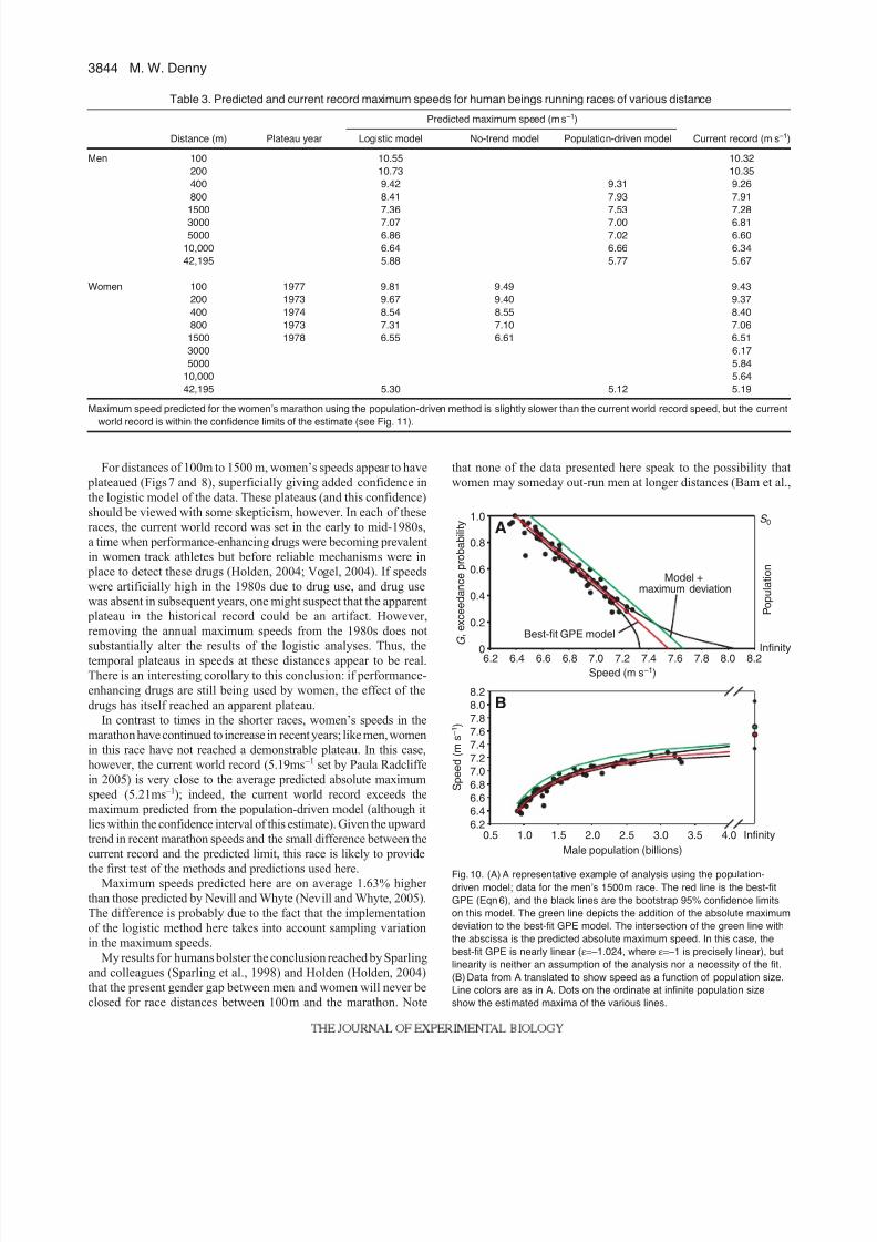
Table 3. Predicted and current record maximum speeds for human beings running races of various distance


Distance (m) Plateau year Logistic model No-trend model Population-driven model Current record (m s –1)

Men 100 10.55 10.32

200 10.73 10.35

400 9.42 9.31 9.26

800 8.41 7.93 7.91

1500 7.36 7.53 7.28

3000 7.07 7.00 6.81

5000 6.86 7.02 6.60

10,000 6.64 6.66 6.34

42,195 5.88 5.77 5.67

Women 100 1977 9.81 9.49 9.43

200 1973 9.67 9.40 9.37

400 1974 8.54 8.55 8.40

800 1973 7.31 7.10 7.06

1500 1978 6.55 6.61 6.51

3000 6.17

5000 5.84

10,000 5.64

42,195 5.30 5.12 5.19

Maximum speed predicted for the womenʼs marathon using the population-driven method is slightly slower than the current world record speed, but the currentworld record is within the confidence limits of the estimate (see Fig. 11).

6.2 6.4 6.6 6.8 7.0 7.2 7.4 7.6 7.8 8.0 8.2

G ,

e x c

e e

d a n c e p r o

b a

b i l i t y

0

0.2

0.4

0.6

0.8

1.0

P o p u

l a t i o n

Infinity

Best-fit GPE model

Model +maximum deviation

A

Infinity

S 0

0.5 1.0 1.5 2.0 2.5 3.0 3.5 4.0

S p e e

d ( m

s –

1 )

6.2

6.4

6.6

6.8

7.0

7.2

7.4

7.6

7.8

8.0

8.2B

Speed (m s–1)

Male population (billions)

Fig.10. (A) A representative example of analysis using the population-

driven model; data for the menʼs 1500m race. The red line is the best-fit

GPE (Eqn 6), and the black lines are the bootstrap 95% confidence limits

on this model. The green line depicts the addition of the absolute maximum

deviation to the best-fit GPE model. The intersection of the green line with

the abscissa is the predicted absolute maximum speed. In this case, the

best-fit GPE is nearly linear (ε= –1.024, where ε= –1 is precisely linear), but

linearity is neither an assumption of the analysis nor a necessity of the fit.

(B)Data from A translated to show speed as a function of population size.

Line colors are as in A. Dots on the ordinate at infinite population size

show the estimated maxima of the various lines.




1997). Similarly, my results are consistent with the conclusion

reached by Yang (Yang, 1975) that increases in human population

will have only a minor effect on speed.

Evolution

Is it reasonable to suppose that the evolution of speed in horses has

reached its limits? In a restricted sense, the answer is yes. The

equipment used in horse racing, and the surfaces of the tracks on

which these races are contested, did not change appreciably during

the years when speeds were increasing in the Triple Crown races,and they have not changed since. Nor were there any apparent

breakthroughs in training or nutrition that led to the increases in speed

in thoroughbreds in the first half of the twentieth century. It seems

likely, then, that the initial increase in speed in horses was due

primarily to selective breeding. If this is true, evidence from the Triple

Crown races suggests that the process of selective breeding of

thoroughbreds (as practiced in the US) is incapable of producing a

substantially faster horse: despite the efforts of the breeders, speeds

are not increasing, and current attempts to breed faster horses may

instead be producing horses that are more fragile (Drape, 2008). The

fastest speed in two of the Triple Crown races was set in 1973 by thesame horse, Secretariat, and he was initially credited with a speed

equal to the record in the third race (the Preakness Stakes) as well.

(The timer malfunctioned in that race, however, and Secretariat’s

subsequently established official speed is slightly slower.) Thus,

Secretariat approached the predicted absolute maximum speeds in all

three of his Triple Crown races and therefore may represent a good

approximation of the ultimate individual thoroughbred in races

1.25–1.5miles long.

In a larger sense, however, the equine data presented here are

preliminary at best. It may well be possible that different criteria

for selective breeding of horses could produce a faster animal.

Thoroughbreds have been recognized as a separate breed since

the 1700s, and regulation of the breed has constrained its gene

pool: thoroughbreds are less genetically diverse than other breedsof horses (Cunningham et al., 2001). The breed is effectively a

closed lineage descended from as few as 12–29 individuals

(Cunningham et al., 2001; Hill et al., 2002), and 95% of the

paternal lineages in present-day thoroughbreds can be traced to

a single stallion, The Darley Arabian. Selective breeding starting

with different equine stock could perhaps yield faster horses. In

this sense, then, the results presented here do not necessarily

address the question of the maximum speed for the species Equus

cabillus.

The same arguments apply to greyhounds. Greyhounds have been

bred for speed since antiquity, and the results presented here show

a clear plateau in the ability of current selective breeding to produce

a faster greyhound. However, given the extraordinary malleability

of canine morphology (which includes everything from Chihuahuasto Great Danes), it is quite possible that different breeding strategies

(perhaps starting with a different breed of dog) could produce a

faster Canus familiaris.

Human running

log10 distance (m)

1.5 2.0 2.5 3.0 3.5 4.0 4.5 5.0

S p e e

d ( m

s –

1 )

4

6

8

10

12100 200 400 8001.5k 3k 5k 10k Marathon

Fig.11. Summary of human running data for distances 100m to 42,195 m.

Solid lines are the current world records for men (blue) and women (red).

Estimates from the no-trend approach are shown by the circles; estimates

from the logistic approach are shown by the squares; and estimates from

the population-driven approach are shown by the diamonds. Error bars

show the 95% range of the extreme-value estimate of absolute deviations.Estimates based on 100year return values (rather than absolute maxima)

are denoted with open symbols. For clarity, symbols are staggered slightly

along the abscissa.

Table 4. Current and predicted human records for standard race distances

Average predicted Current record Average predicted absolute Average increase

Distance (m) Current world record absolute world record speed (ms –1) maximum speed (m s –1) in speed (%)

Men 100 9.69 s 9.48 s 10.32 10.55 2.22

200 19.30 s 18.63 s 10.35 10.73 3.68

400 43.18 s 42.73 s 9.26 9.36 1.06

800 1:41.11 1:38.04 7.91 8.17 3.22

1500 3:26.00 3:21.42 7.28 7.45 2.29

3000 7:20.67 7:06.42 6.81 7.04 3.34

5000 12:37.35 12:00.8 6.60 6.94 5.0910,000 26:17.53 25:03.4 6.34 6.65 4.93

42,195 2:03.59 2:00.47 5.67 5.83 2.72

Women 100 10.61 s* 10.39 s 9.43 9.65 2.38

200 21.34 s 20.99 s 9.37 9.53 1.73

400 47.60 s 46.75 s 8.40 8.54 1.65

800 1:53.28 1:50.83 7.06 7.20 2.01

1500 3:50.46 3:47.92 6.51 6.58 1.12

3000 8:06.11 6.17

5000 14:16.63 5.84

10,000 29:31.78 5.64

42,195 2:15.25 2:14.97 5.19 5.21 0.36

*The official world record is 10.49 s, but there is compelling evidence that that race was wind aided (Pritchard and Pritchard, 1994).



3846

Once again, the situation is less clear for humans. Unlike the

apparent case in horses and dogs, human runners have recently

benefited from substantial improvements in training, equipment and

nutrition. In some cases (women’s sprints), these benefits may have

reached their own limits. But in other races, continued improvement

in training, equipment and nutrition may well be contributing to the

continued increase in race speeds. Because these effects are

inextricably entwined with the historical race data, the predictions Imake here may be biased. In essence, these predictions assume that

historical trends in training, equipment and nutrition (whatever they

are) will continue into the future. It is always dangerous to make such

assumptions. Competitive swimming provides an example of this

potential effect: improvement in the design of full-body swimsuits (a

breakthrough not contemplated 10years ago) contributed to a rash of

recent world records, 25 in the Olympics of 2008 alone. Until we

know more about the mechanisms of improvement in training,

equipment and nutrition, and more about their actual role in the

historical running record, the magnitude of their effects on future

running speeds will remain uncertain, and the predictions made here

must be used cautiously.

And then there is the subject of artificial performance enhancement,

which inevitably leads to philosophical questions pertaining to thedefinition of absolute maximum speed. For example, how should we

define ‘male’, ‘female’ and even ‘human’ for the purposes of this

study? If a woman artificially enhances the concentration of

testosterone in her body, a large number of changes accrue that make

her physiologically more like a man and capable of higher speeds

(e.g. Holden, 2004). In this altered state, she may exceed any limits

that might exist for unaltered individuals. At what point should such

a hormonally enhanced woman no longer count as a woman in the

analysis of maximum female human speed? Stanislawa Walasiewicz

(Stella Walsh) provides an intriguing example. She was the preeminent

female sprinter of the 1930s, posting times that were not matched

until the 1950s. She married in 1956 and was subsequently shot and

killed during a supermarket robbery, where she was an innocent

bystander. An autopsy revealed that (unbeknownst to her) she was ahermaphrodite, possessing both ovaries and testes. Presumably the

anabolic steroids produced by her testes contributed to her athletic

success (Lawson, 1997), but had she not been murdered, we would

never have known. Where should she be placed in the record books?

Even more vexing questions await us in the future. For example, the

potential exists to genetically engineer human athletes for enhanced

performance (e.g. Vogel, 2004). At what point does a genetically

altered person no longer count as human? (Similar questions can be

raised regarding drugs and gender in greyhounds and horses.)

For scientific purposes, these sticky questions can in large part

be circumvented through the use of arbitrary definitions. As long

as one defines practical criteria for ‘female’, ‘male’ or ‘human’

in formulating a mechanical/physiological model of locomotion,

the predictions of that model can be compared with an appropriateset of test organisms. For present purposes, let us define a

greyhound, thoroughbred or human (male or female) as an

individual performing without drug or genetic enhancement. If

drugs have contributed to the winning speeds in the races used

here, speeds in the absence of these drugs would presumably have

been slower. Thus, if we could definitively account for the effect

of drugs in the historical record, the estimated maximum speeds

I predict for unadulterated animals would, if anything, be slower,

and my estimates are in this sense conservatively fast.

A similar conclusion applies to possible variation in the fraction

of the overall human population that participates in running races.

Recall that the analysis of the effect of population size on maximum

M. W. Denny

speed assumed that f , a fixed (although unspecified) fraction of all

men and women, runs each year. In reality, it seems likely that f has

increased through time as awareness of the sport has spread and more

prize money has been made available. In particular, the fraction of

women competing in running races has probably increased in recent

decades. However, if we could take the presumed increase in f into

account in this analysis, the effect would be to reduce the predicted

maximum speed. (See Appendix 2 for an explanation.) In this respect,my results are again conservatively fast.

Some cynics have suggested that the problem of artificial

enhancement in sports should be ‘solved’ by simply making drug

and genetic enhancement legal. If such enhancement is allowed,

the question of maximum human running speed becomes much

more difficult to answer. On the one hand, it seems likely that

humans have been, and still are, clandestinely employing

performance-enhancing drugs despite the ban on their use. If so,

the efficacy of these drugs is questionable: e.g. women’s speeds

in sprint races appear to have plateaued. On the other hand, it is

impossible to rule out the possibility that new drugs or genetic

enhancement could do for running what full-body swim suits have

done for swimming: provide the means for dramatic improvement.

In that case, the maximum speeds estimated here could be low.

What limits speed?

The analysis presented here deals solely with the results of

competitive races, not with the factors that caused a certain

individual to win or lose. In this respect, my results are as

unsatisfying as those of previous statistical analyses: they tell us

that speed has limits, but not what accounts for these limits.

Nonetheless, the pattern of estimated maximal speeds provides

information of potential value to physiologists and biomechanicians.

It seems unlikely that a single mechanical or physiological factor

could account for the limit to speed at all distances. The height and

mass of elite runners differs among race distances (Weyand and

Davis, 2005) as does the ability of aerobic capacity to predict speeds

(Weyand et al., 1994; Weyand et al., 1999). It is striking, then, thatthe predicted scope for increased speed in humans is similar across

distances ranging from 100m to 42,195m (Fig.11; Table4). This

distance-independent scope for increase suggests that some sort of

higher order constraint may act on the suite of physiological and

mechanical factors to limit speed.

Context

The likelihood that there are limits to speed should not diminish

the awe with which we view the performance of dogs, horses and

humans. For example, a women running the estimated absolute

fastest speed for 100 m would have beaten the world’s fastest male

in 1955, a feat that would have astounded contemporary spectators.

The predicted maximum speed (5.83ms –1) for a man running a

marathon (42.2km) would have been fast enough to beat the greatEmil Zatopek in his world’s best 10km race in 1954. Those in the

stands watching that race could not have imagined someone besting

Zatopek by 16 s, and then simply continuing at that winning pace

for another 32.2km.

APPENDIX 1

Notes on the historical records

Horses

Until 1991, Triple Crown races were timed by hand to the nearest

0.2s; since then they have been timed electronically to the nearest

0.01s. I have made no correction for the shift from hand to electronic

timing.




Humans

In some women’s races, the earliest data are extremely variable,

perhaps because so few women participated in the sport at that time.

For the 100 m race, women’s data prior to 1931 were not used. For

the 400m race, data prior to 1928 were not used.

World’s best times by a individual later proven to be using

performance-enhancing drugs were deleted from the record; in

those years, the second-best time was used. Times posted byindividuals of uncertain gender (as noted by the ATFS) were not

used; second-best times were substituted. The current women’s

100m world record (10.49s) was set by Florence Griffith Joyner

in 1984, but there is compelling evidence that that race was wind

aided (Pritchard and Pritchard, 1994). I have replaced this world’s

best for 1984 with a time of 10.61 s (Griffith Joyner’s second-best

time for that year).

Until the 1970s, human races were timed by hand. Because of

the slight delay in starting a watch (due to human response time)

and the potential for an early stop as an official anticipates the finish,

hand times are slightly shorter than corresponding electronic times

by approximately 0.165s. This difference is negligible for races of

400m and longer, but can be a substantial factor in 100m and 200 m

races. Here, I have added 0.165s to hand-timed 100m and 200mtimes. For 2–3years during the switch-over from hand to electronic

timing, world’s best times were recorded for both methods, and both

hand-timed results (plus 0.165 s) and electronic results have been

included here.

A race of 220yards is very similar in length to a race of 200m

(220yards=201.168m). The ATFS has reconciled the two races by

recording 220yard times minus 0.1s as equivalent to 200m times

for both men and women, and I follow this convention here.

Similarly, I accept 440yard times minus 0.3s as equivalent to 400m

times.

APPENDIX 2

Relating population size to exceedance probability

The generalized Pareto equation (GPE) is traditionally expressedas a cumulative probability distribution:

where P (V ) is the probability that the maximum speed in a randomly

chosen sample of size S 0 is ≤V (Coles, 2001). For the present

purposes, it is more convenient to work with 1– P (V )=G(V ), where

G(V ) is the chance of getting a sample maximum speed >V :

How many samples of size S 0 would one have to take (on average)to get a maximum speed >V ? From the laws of probability (Feller,

1968; Denny and Gaines, 2000) it can be shown that this exceedance

number E is:

If each sample has S 0 individuals and we need E samples (on

average) to get a maximum speed >V , the overall number of

individuals we need to sample to exceed V is:

S = ES 0 =S 0

G(V ). (A4)

E =1

G(V ). (A3)

G(V ) = 1+ εV − u

σ

−1/ε

. (A2)

P (V ) = 1− 1+ εV − u

σ

−1/ε

, (A1)

Rearranging, we solve Eqn A4 for G(V ):

Upon inserting Eqn A5 into Eqn A2, we see that:

If, in a given year, the world population of (for example) womenis N and fraction f are runners, S = fN women run the race that year.

When measured in units of S 0, the number of ‘samples’ of maximum

speed we take in a given year is therefore S /S 0. If f is constant across

years, S 0/S = N 0/ N where N 0 is the world population in the year in

which S 0 was measured. Thus:

In this fashion, N 0/ N (and hence G) can be estimated from records

of world population for each measured V . Plotting G as a function

of V provides an estimate of the exceedance function described by

Eqn 6 in the text. This is the recipe for estimating u, σ and ε discussed

in the text.It is possible that the fraction of the human population sampled

by competition (especially the fraction of women) has increased

over the last century. If so, maximum speeds predicted using the

population-driven model are too high: estimates of cumulative

probability incorporating an increasing fraction of runners would

yield lower G values for recent years than those shown here, thereby

lowering the estimates for extrapolated maximum speed (see

Fig.A1).

APPENDIX 3

Details of the statistical results

Details of the statistical results are given in Tables A1 to A8.

G(V ) = N 0

N = 1+ ε

V − u

σ

−1/ε

. (A7)

S 0

S = 1+ ε

V − u

σ

−1/ε

. (A6)

G(V ) =S 0

S . (A5)

Speed (m s–1)

6.8 7.0 7.2 7.4 7.6 7.8 8.0 8.2 8.4 8.6 8.8

G ,

e x c e e

d a n c e p r o

b a

b i l i t y

0

0.2

0.4

0.6

0.8

1.0

P o p u

l a t i o n

S 0

Infinity

Fig. A1. If f , the fraction of individuals that run a particular race,

increases through time, the actual population of runners associated with

a given measured maximum speed (open dots) is higher than that

supposed by the calculations made here (solid dots). A larger population

corresponds to a smaller probability of exceedance (e.g. the green

arrow). Thus, if probabilities were to be adjusted for an increase in f

(open dots) the estimated absolute maximum speed would be reduced

(the blue arrow).



3848 M. W. Denny

Table A1. Parameters for the GEV (Eqn 1) for the plateau portion of the historical record for US Triple Crown races

Plateau begins Probability a b c

Kentucky Derby 1949 >0.882 –0.2826 16.4077 0.1577

Preakness Stakes 1971 >0.867 –0.4390 16.5970 0.1392

Belmont Stakes 1973 >0.232 –0.2004 16.2169 0.1631

GEV, generalized extreme value; a , shape parameter; b , location parameter; and c , scale parameter (see Eqn 1). All values for a are significantly less than 0

(P <0.05). The probability cited here is the likelihood that any calculated correlation between speed and year is due to chance alone.

Table A2. Parameters of the logistic model for the US Triple Crown races

Race mx Low 95% High 95% mn k t a b c

Kentucky Derby 16.498 16.387 16.609 14.925 0.056 1913.13 –0.4503 –0.0725 0.2906

Preakness Stakes 16.644 16.575 16.713 15.913 0.121 1954.51 –0.3288 –0.0520 0.1637

Belmont Stakes 16.281 16.230 16.333 3.145 0.053 1862.24 –0.2421 –0.0586 0.1640

The 95% confidence limits are given for mx, the estimated maximum of the logistic model. Values for mn (minimum fastest speed), k (shape parameter) and t

(location parameter) of the logistic model are best-fit estimates. Values shown for a , b and c of the GEV (Eqn 1) are best-fit estimates. All values for a are

significantly less than 0 (P <0.05).

Table A3. Parameters for the GEV (Eqn 1) for the plateau portion of the historical record for greyhound races

Plateau begins Probability a b c

English Oaks 1971 >0.132 –0.5230 16.526 0.1631

English Grand National 1971 >0.606 –0.3023 16.105 0.2180

English Derby 1966 >0.922 –0.4165 16.662 0.1607

All values for a are significantly less than 0 (P <0.05). The probability cited here is the likelihood that any calculated correlation between speed and year is due

to chance alone.

Table A4. Parameters of the logistic model for greyhound races

Race mx Low 95% High 95% mn k t a b c

English Oaks 16.602 16.454 16.750 5.751 0.051 1879.21 –0.4734 –0.0468 0.1689

English Grand National 16.205 16.059 16.351 8.401 0.055 1889.88 –0.2597 –0.0650 0.1791

English Derby 16.713 16.636 16.789 8.489 0.079 1901.25 –0.3630 –0.0426 0.1402

The 95% confidence limits are given for mx, the estimated maximum of the logistic model. Values for mn, k and t of the logistic model are best-fit estimates.

Values shown for a , b and c of the GEV (Eqn 1) are best-fit estimates. All values for a are significantly less than 0 (P <0.05).

Table A5. Parameters for the GEV (Eqn 1) for the plateau portion of the historical record for womenʼs races

Distance (m) Plateau begins Probability a b c

100 1977 >0.801 0.1506 9.2278 0.0400

200 1973 >0.846 –0.1516 9.1046 0.0901

400 1974 >0.695 0.0293 8.0870 0.0935

800 1973 >0.869 –0.1541 6.9078 0.0580

1500 1978 >0.987 0.1495 6.3156 0.0450

For the 200m and 800 m races, all values for a are significantly less than 0 (P <0.05); a is significantly >0 for the 100m and 1500m races and indistinguishable

from 0 for the 400 m race. The probability cited here is the likelihood that any calculated correlation between speed and year is due to chance alone.

Table A6. Parameters of the logistic model for various human races

Distance (m) mx Low 95% High 95% mn k t a b c

Men 100 10.330 10.165 10.495 9.439 0.063 1971.65 –0.3156 –0.0256 0.0771

200 10.186 10.050 10.322 9.340 0.073 1962.95 –0.1859 –0.0486 0.1107

400 9.160 9.035 9.285 8.262 0.057 1949.31 –0.3090 –0.0298 0.0884

800 7.839 7.758 7.920 6.977 0.059 1947.94 –0.0940 –0.0274 0.0053

1500 7.251 7.147 7.356 6.313 0.061 1955.12 –0.5325 –0.0141 0.06763000 6.868 6.610 7.127 5.353 0.036 1942.45 –0.2803 –0.0221 0.0619

5000 6.589 6.454 6.724 5.533 0.052 1956.90 –0.1796 –0.0226 0.0519

10,000 6.350 6.208 6.492 5.114 0.048 1953.78 –0.1678 –0.0233 0.0528

42,195 5.612 5.518 5.706 4.234 0.065 1948.28 –0.3599 –0.0315 0.1070

Women 100 9.297 9.222 9.373 8.277 0.109 1963.27 –0.1568 –0.0378 0.0858

200 9.214 9.112 9.317 7.699 0.090 1955.42 –0.2468 –0.0457 0.1227

400 8.174 8.097 8.251 6.732 0.127 1960.64 0.0303 –0.0512 0.0838

800 7.006 6.909 7.103 5.425 0.086 1952.14 –0.3525 –0.0368 0.1200

1500 6.355 6.325 6.385 5.372 0.277 1967.45 0.0020 –0.0281 0.0482

42,195 5.028 4.974 5.082 0.775 0.121 1959.98 –0.3159 –0.0324 0.0967

The 95% confidence limits are given for mx, the estimated maximum of the logistic model. Values for mn, k and t of the logistic model are best-fit estimates.

Values shown for a , b and c of the GEV (Eqn 1) are best-fit estimates. With the exception of the 400m and 1500m races for women, all values for a are

significantly less than 0 (P <0.05). For womenʼs 400m and 1500m races, a is indistinguishable from 0.




I thank S. Davis, Secretary of the ATFS; S. Ito of the LA84 Foundation Library; C.Leavy and D. J. Histon of the Irish Stud Book; D. Kohrs and the MinneapolisPublic Library for assistance in compiling race data; and J. M. Gosline forsuggesting horses and greyhounds as experimental subjects.

REFERENCESAlexander, R. M. (2003). Principles of Animal Locomotion. Princeton, NJ: Princeton

University Press.Association of Track and Field Statisticians (1951-2006). ATFS Annual. Worcester,

UK: SportsBooks.Bam, J. T., Noakes, D., Juritz, J. and Steven, S. C. (1997). Could women outrun

men in ultramarthon races? Med. Sci. Sports Exerc . 29, 244-247.Biewener, A. A. (1989). Support in mammals: limb posture and muscle mechanics.

Science 245, 45-48.Biewener, A. A. (1990). Biomechanics of mammalian terrestrial locomotion. Science

250, 1097-1103.Biewener, A. A. (2003). Animal Locomotion . Oxford: Oxford University Press.Blanco, R. E., Gambini, R. and Fariña, R. A. (2003). Mechanical model for

theoretical determination of maximum running speed in mammals. J. Theor. Biol.222, 117-125.

Cohen, J. (1995). How Many People Can the Earth Support? New York: Norton.Coles, S. (2001). An Introduction to Statistical Modeling of Extreme Values. London:

Springer-Verlag.Cunningham, E. P., Dooley, J. J., Splan, R. K. and Bradley, D. G. (2001).

Microsatellite diversity, pedigree relatedness and the contributions of founderlineages to thoroughbred horses. Anim. Genet. 32, 360-364.

Denny, M. W. and Gaines, S. (2000). Chance in Biology . Princeton, NJ: PrincetonUniversity Press.

Drape, J. (2008). Breeding for speed, ignoring durability. New York Times , May 11.Efron, B. and Tibshirani, R. J. (1993). An Introduction to the Bootstrap . Boca Raton,

FL: CRC Press.Farley, C. T. (1997). Maximum speed and mechanical power output in lizards. J. Exp.

Biol. 200, 2189-2195.

Feller, W. (1968). An Introduction to Probability Theory and its Applications. 3rd Edn.New York: John Wiley.

Gaines, S. and Denny, M. W. (1993). The largest, smallest, highest, lowest, longestand shortest: extremes in ecology. Ecology 74, 1677-1692.

Hill, E. W., Bradley, D. G., Al-Barody, M., Ertugrul, O., Splan, R. K., Zakharov, I.and Cunningham, E. P. (2002). History and integrity of the thoroughbred dam linesrevealed in equine mtDNA variation. Anim. Genet. 33, 287-294.

Holden, C. (2004). An everlasting gender gap? Science 305, 639-640.Hutchison, J. R. and Garcia, M. (2002). Tyrannosaurus was not a fast runner. Nature

415, 1018-1021.

Iriarté-Diaz, J. (2002). Differential scaling of locomotor performance in small and largeterrestrial animals. J. Exp. Biol. 205, 2897-2908.

Jones, J. H. and Lindstedt, S. L. (1993). Limits to maximal performance. Ann. Rev.Physiol . 55, 547-569.

Katz, R. W., Brush, G. S. and Parlange, M. B. (2005). Statistics of extremes:modeling ecological disturbances. Ecology 86, 1124-1134.

Keller, J. B. (1973). A theory of competitive running. Phys. Today 26, 42-46.Kök, N., Magnusson, R., Potts, D. H. and Quercetani, R. L. (1995). Track and Field

Performances Through the Years. Vol. 3, 1945-1950. Trowbridge, UK: Association ofTrack and Field Statisticians.

Kök, N., Magnusson, R., Potts, D. H. and Quercetani, R. L. (1999). Track and Field Performances Through the Years. Vol. 4, 1921-1928. Trowbridge, UK: Association ofTrack and Field Statisticians.

Magnusson, R., Potts, D. H. and Quercetani, R. L. (1991). Track and Field Performances Through the Years. Vol. 2, 1937-1944. Trowbridge, UK: Association ofTrack and Field Statisticians.

Lawson, G. (1997). World Record Breakers in Track and Field Athletics. Champaign,IL: Human Kinetics.

Nevill, A. M. and Whyte, G. (2005). Are there limits to running world records? Med.Sci. Sports Exerc. 37, 1785-1788.

Pritchard, W. G. and Pritchard, J. K. (1994). Mathematical models of running. Am.Sci. 82, 546-553.

Quercetani, R. L. and Magnusson, R. (1988). Track and Field Performances Through the Years. Vol. 1, 1929-1936. Trowbridge, UK: Association of Track and FieldStatisticians.

Sparling, P. B., OʼDonnell, E. M. and Snow, T. K. (1998). The gender difference indistance running performance has plateaued: an analysis of world rankings from1980 to 1996. Med. Sci. Sports Exerc. 30, 1725-1729.

Tatem, A. J., Guerra, C. A., Atkinson, P. M. and Hay, S. I. (2004). Momentous sprintat the 2156 Olympics? Nature 432, 525.

Tibshirani, R. (1997). Who is the fastest man in the world? Am. Stat. 51, 106-111.Vogel, G. (2004). A race to the starting line. Science 305, 632-635.Weyand, P. G. and Davis, J. A. (2005). Running performance has a structural basis.

J. Exp. Biol. 208, 2625-2631.Weyand, P. G., Cureton, K., Conley, D. S., Sloniger, M. A. and Liu, Y. L. (1994).

Peak oxygen deficit predicts sprint and middle-distance performance. Med. Sci.

Sports Exerc . 26, 1174-1180.Weyand, P. G., Lee, C. S., Martinez-Ruiz, R., Bundle, M. W., Bellizzi, M. J. andWright, S. (1999). High-speed running performance is largely unaffected by hypoxicreductions in aerobic power. J. Appl. Physiol. 68, 2059-2064.

Weyand, P. G., Sternlight, D. B., Bellizzi, M. J. and Wright, S. (2000). Faster toprunning speeds are achieved with greater ground forces not more rapid legmovements. J. Appl. Physiol. 89, 1991-1999.

Whipp, B. J. and Ward, S. A. (1992). Will women soon outrun men? Nature 355, 25.Yang, M. C. K. (1975). On the distribution of the inter-record times in an increasing

population. J. Appl. Probab. 12, 148-154.

Table A7. Correlation between population size and speed in womenʼs races

Distance (m) Plateau begins (population, billions) Probability

100 2.393 >0.369

200 2.184 >0.146

400 2.063 >0.703

800 2.063 >0.334

1500 2.143 >0.987

The probability cited here is the likelihood that any calculated correlation between speed and population size is due to chance alone.

Table A8. Parameters of the population-driven model for various human races

Estimated

Distance (m) model max. Low 95% High 95% ε σ u a b c

Men 400 9.31 9.13 9.71 –1.314 1.358 8.273 –0.3140 –0.0299 0.0892

800 7.93 7.85 8.08 –1.566 1.367 7.055 –0.0918 –0.0277 0.0560

1500 7.53 7.32 8.08 –1.024 1.183 6.377 –0.5427 –0.0138 0.0679

3000 7.00 6.82 7.31 –1.088 1.217 5.885 –0.2873 –0.0222 0.0633

5000 7.02 6.70 7.84 –0.775 1.082 5.624 –0.1919 –0.0223 0.0522

10,000 6.66 6.40 7.27 –0.933 1.303 5.264 –0.1850 –0.0229 0.0535

42,195 5.77 5.65 5.99 –1.616 2.428 4.269 –0.3555 –0.0317 0.1058

Women 42,195 5.12 5.03 5.30 –4.266 7.948 3.259 –0.3334 –0.0325 0.1012

The 95% confidence limits are given for the estimated maximum of the model [u –(σ/ε)]. Values for σ, ε and u of the GPE are best-fit estimates. Values shown

for a , b and c of the GEV (Eqn 1) are best-fit estimates. All values for ε and a are significantly less than 0 (P <0.05).



Inside Ji

100m WORLD RECORD COULDGO AS LOW AS 9.48s2008 was a great summer for sports’ fans.World records tumbled at the BeijingOlympics. Usain Bolt shattered both the100m and 200m world records, knockingtenths of a second off each. People have

been getting faster and faster over the lastfew decades, which made marathon runner Mark Denny, from Stanford University,wonder whether last century’s massiveincrease in population could account for these dramatic improvements. He alsowondered whether there are absolute limitson running speeds and, if so, how close arewe to them? Suspecting that there are,Denny decided to scrutinise the running

performances of humans and two other famous racing species, dogs andthoroughbred horses, to find how closemodern runners are to their species’ peak

performances (p. 3836).

Having found records dating back to the1920s for dogs and the 19th century for humans and thoroughbreds, Denny lookedto see whether there were any clear trends;had any of the species’ performancesalready levelled off? Plotting the annual toprunning speeds for all three species over theyears, it was clear that racing horses anddogs have already reached a plateau. Therehas been no improvement in thethoroughbred’s speed in the KentuckyDerby since the 1940s and two other major US races since the 1970s, while dogs’

performances also levelled out in the 1970s.The increasing dog and thoroughbred

populations hadn’t improved the animals’ performances. However, ‘chance might stillturn up a faster animal,’ says Denny and he

predicts that thoroughbreds could improvetheir top speeds by as much as 1% in the2012m Kentucky Derby, eventually

peaking at a top speed of just over 17ms –1.

For humans the results were complicated bythe different distances that people race.Looking at the speeds of male race winnersthrough the years, it seems as if men stillhaven’t reached their top speeds at anydistance and Denny predicts that male 100msprinters could one day get the record down

to an incredible 9.48s, running 0.23ms –1

faster than Usain Bolt’s current world recordof 9.69s. Meanwhile, female sprinters’ topannual speeds levelled off in the 1970s,suggesting that any improvement in their speed was not due to a population increase.However, Denny suspects that femalesprinters have room for improvement too,and predicts that they could eventuallyknock more than 0.4s of the current 100mworld record to cover the distance in 10.19s.

Looking at marathon runners, Denny predicts that males could cut the current

world record, held by Haile Gebrselassie, by between 2min7s and 4 min23s. Andwhen he calculates the top speed that ahuman female marathon runner couldachieve, Denny suspects that women couldeventually cross the 42,195 m finishing linein 2h12min41s. He adds that Paula

Radcliffe’s current world record of 2h15min25s is very close to his average prediction for the maximum marathonspeed and suspects that female marathonrunners could be the first group to approachhis predictions and test whether they hold.

Denny is pleased to have shown that it is possible to calculate the absolute limits tospeed of running animals ranging fromhumans to thoroughbred horses. However,he emphasises that we have no idea whataspect of physiology restricts runners’

performances, and is keen to find out whatwill prevent future gold medal winnersfrom breaking Denny’s Limits.

10.1242/jeb.027201

Denny, M. W. (2008). Limits to running speed in dogs,horses and humans. J. Exp. Biol. 211, 3836-3849.

I n s i

d e J E

B

Inside JEB is a twice monthlyfeature, which highlights the keydevelopments in The Journal of Experimental Biology . Written byscience journalists, the shortreports give the inside view of

the science in JEB.

BACKSWIMMERS REGULATEBUOYANCY WITHHAEMOGLOBIN

Backswimmers in the pool are a commonsight in Australia, according to PhilipMatthews from the University of Adelaide.It was only when Matthews startedinvestigating these curious little insects inmore detail that he began to appreciate howunique they are. For example, most divinginsects are positively buoyant so bob

around at the surface or actively swim toremain submerged. But backswimmers canachieve neutral buoyancy and float atdepths of up to 0.5m, which madeMatthews wonder how backswimmersmaintain neutral buoyancy when other insects have to struggle to plumb thedepths. Knowing that diving insects,including backswimmers, always take a

bubble of air down with them for oxygenwhen they become submerged and that

backswimmers have extraordinarily highlevels of oxygen-carrying haemoglobin,Matthews and his supervisor Roger

Documents

Denny Limits to Running Speeds JEB 2008