Dengue Fever with Two Strains in Thailand

Index Terms—Dengue, strains, reproduction number,

mathematical model, Thailand.

I. INTRODUCTION Dengue is one of the several emerging tropical diseases

which progressively spread geographically to virtually all tropical countries. It is transmitted by the bite of an Aedes mosquito infected with any one of the four dengue viruses. Theses infected mosquitoes pass the disease to susceptible humans. It is known individuals who recover from one serotype become permanently immune to it, but may become partially-immune or temporarily-immune to the other serotypes [1]-[3]. Epidemiological evidence suggests that an important risk factor for dengue is the presence of preexisting antibodies at subneutralizing level [4]. This led to the formulation of secondary infection or immune enhancement hypothesis.

In Thailand, dengue epidemics have occurred every year in the last 40 years [1]. Thus, the model of dengue with two strains is formulated for predicting the transmission dynamics of dengue in Thailand.

II. MODEL DESCRIPTION The model is formulated based on the following

assumptions. 1) The total human population at time ,t denoted

by ( ),HN t is divided into twelve sub-populations, so that

1 2 1 2 1

2 12 21 12 21 22

( ) ( ) ( ) ( ) ( ) ( ) ( )( ) ( ) ( ) ( ) ( ) ( ).

H H H H H H H

H H H H H H

N t S t E t E t I t I t R tR t E t E t I t I t R t= + + + + + +

+ + + + +

(1) 2) Once a mosquito is infected it never recovers and it

cannot be reinfection with a difference serotype of virus. Secondary infection, therefore, may take place only in human population [1]. Thus, the total mosquito population at time ,t denoted by ( ),vN t is split into five sub-populations, so that

1 2 1 2( ) ( ) ( ) ( ) ( ) ( ).V V V V V VN t S t E t E t I t I t= + + + + (2)

3) The recruitment rate of human and vector populations

are denoted by HΠ and ,VΠ respectively. 4) Flow from the susceptible to the infected class of both

populations (human and mosquito), for each strain, depend on the biting rate of the mosquitoes, the transmission probabilities, as well as the number of infectives and susceptibles of each population [5], [6]. It assumed that the transmission probability from an infected human to a susceptible mosquito must equal the transmission probability from an infected mosquito to a susceptible human ( ) .VH HVρ ρ= Then, the rate of infection with strain 1 or strain 2 per susceptible human for primary infection are given by

( )1 1 1 1 ,HVV V V

HNC

E I= +ηβ (3)

( )2 2 2 2 ,HVV V V

HNC

E I= +ηβ (3)

where, HV HVC b,= ρ b and HVρ denote the average number of bites per mosquito per unit time and the transmission probability from an infected human to a susceptible mosquito, respectively. The parameter ( )0, 1 , 1, 2,vi i∈ =η account for reduction in transmissibility of exposed mosquitoes relative to infectious mosquitoes.

Similarly, primary infection of mosquito, infection rate per susceptible mosquito with strain 1 or strain 2 are given by

[ ] [ ]( ) [ ] [ ]( )1 1 ,HVv H

H

CES ER IS IR

N= + + +β η (5)

[ ] [ ]( ) [ ] [ ]( )2 2HV

v HH

CSE RE SI RI .

N= + + +β η (4)

where, ( )0, 1 , 1, 2,Hi i∈ =η accounts for the reduction in transmissibility with strain i of exposed human relative to infectious human.

Dengue Fever with Two Strains in Thailand

Sutawas Janreung and Wirawan Chinviriyasit

International Journal of Applied Physics and Mathematics, Vol. 4, No. 1, January 2014

55DOI: 10.7763/IJAPM.2014.V4.255

Manuscript received November 9, 2013; revised January 15, 2014. This

work was supported by the Center of Excellence in Mathematics, the

Commission on Higher Education, Thailand, and the Higher Education

Research Promotion and National Research University Project of Thailand,

Office of the Higher Education Commission.

The authors are with the Department of Mathematics, King Mongkut’s

University of Technology Thonburi, Thung Khru, Bangkok 10140 Thailand

(e-mail: [email protected], [email protected]).

Abstract—In this paper, a mathematical model of dengue

fever with two strains is developed. Analysis of the model

reveals the existence of four equilibrium points, which belong to

the region of biological interest. One of the equilibrium points

corresponds to the disease–free state, the other three equilibria

correspond to the two states where just one strain is present,

and the state where both strain coexist, respectively. The model

has a local asymptotically stable, disease-free equilibrium (DFE)

wherever the maximum of the associated reproduction

numbers of the two strains (denoted by0

sR ) is less than unity.

The proposed model is used to forecast transmission dengue in

Thailand.

5) Immunity to reinfection with a previously experienced serotype hold lifelong. The antibody dependent enhancement (ADE) which is a negative immune reaction occurs after the temporal cross immunity period. Then, secondary infection with strain i are produced at a rate , 1, 2,i i i =λ β where iλ is enhancement multiple for strain .i If 0 1,j≤ <λ primary infection confer partial or total immunity to strain j for 1, 2.j = If 0,j >λ primary infection increase susceptibility to strain j due to immune enhancement. If 1,j =λ primary infections do not alter the susceptibility to secondary infections [7], [8].

6) All subpopulations of human and mosquito die at the same rate Hμ and ,Vμ respectively.

7) The parameter , 1, 2i i =σ denotes the transfer from exposed human to infectious human. The parameter

, 1, 2Vi i =σ denotes the transfer rate from exposed vector to infectious mosquito.

8) The per capita mortality rate of dengue virus with strain i for infectious human and infectious mosquito are

, 1, 2i i =δ and , 1, 2,Vi i =δ respectively. 9) The recovery rate of infectious human with strain i is

, 1, 2.i i =γ With above assumptions, the model of dengue with two

strains described by the following system of nonlinear differential equations

( )1 2 S ,HH H H H

dSS

dt= Π − + −β β μ (7)

( )11 1 1,H

H H HdE

S Edt

= − +β σ μ (5)

( )22 2 2 ,H

H H HdE

S Edt

= − +β σ μ (6)

( )11 1 1 1 1,H

H H HdI

E Idt

= − + +σ γ δ μ (10)

( )22 2 2 2 2 ,H

H H HdI

E Idt

= − + +σ γ δ μ (11)

( )11 1 2 2 1,H

H H HdR

I Rdt

= − +γ λ β μ (7)

( )22 2 1 1 2 ,H

H H HdR

I Rdt

= − +γ λ β μ (8)

( )122 2 2 2 12 ,H

H H HdE

R Edt

= − +λ β σ μ (9)

( )211 1 1 1 21E ,H

H H HdE

Rdt

= − +λ β σ μ (15)

( )122 12 2 2 12 ,H

H H HdI

E Idt

= − + +σ γ δ μ (16)

( )211 21 1 1 21,H

H H HdI

E Idt

= − + +σ γ δ μ (10)

221 21 2 12 22 ,H

H H H HdR

I I Rdt

= + −γ γ μ (11)

( )1 2 ,vv v v v v v

dSS S

dt= Π − + −β β μ (12)

( )11 1 1,v

v v v v vdE

S Edt

= − +β σ μ (13)

( )22 2 2 ,v

v v v v vdE

S Edt

= − +β σ μ (14)

( )11 1 1 1,v

v v v v vdI

E Idt

= − +σ δ μ (22)

( )22 2 2 2 .v

v v v v vdI

E Idt

= − +σ δ μ (15)

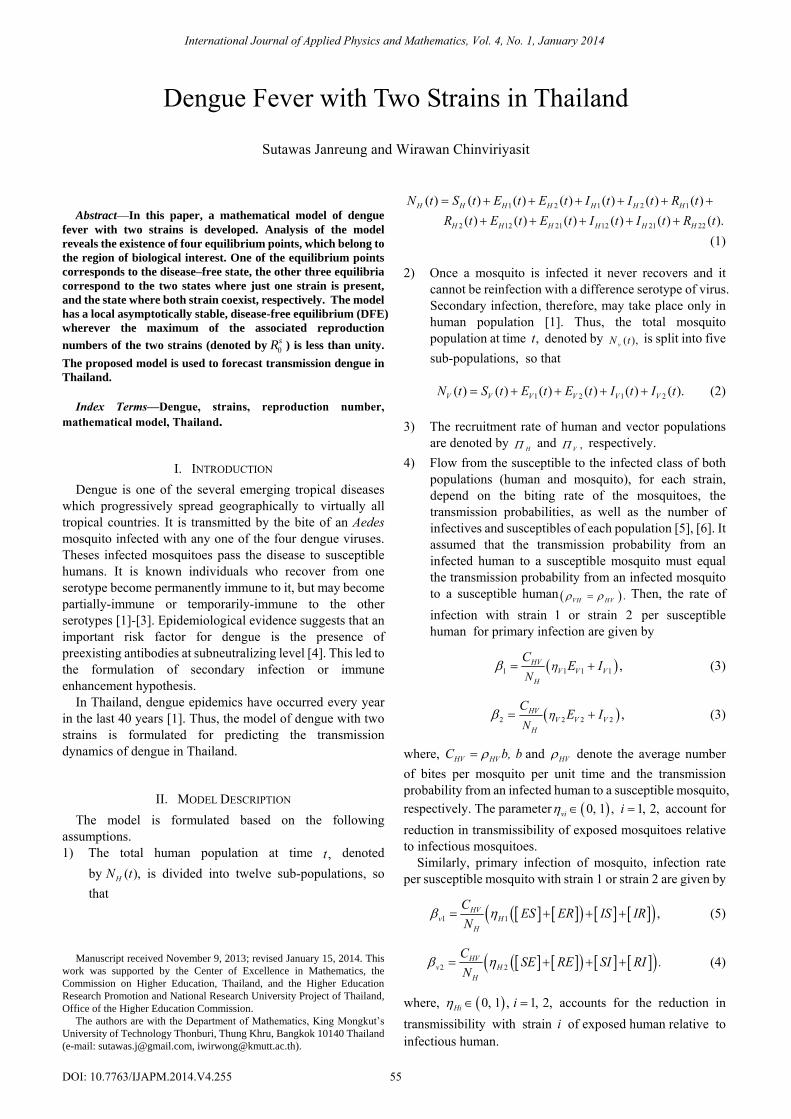
Human population

Vector population

Fig. 1. Schematic diagram of the system (7)-(23).

TABLE I: DESCRIPTION OF VARIABLE OF THE SYSTEM (7)-(23)

Variables Description

HS Humans susceptible to both strains

1HE Humans exposed with strain 1 in primary infection

2HE Humans exposed with strain 2 in primary infection

1HI Humans infected with strain 1 in primary infection

2HI Humans infected with strain 2 in primary infection

1HR Humans recovered with strain 1 in primary infection

2HR Humans recovered with strain 2 in primary infection

12HE Humans exposed to strain 2 in secondary infection

21HE Humans exposed to strain 1 in secondary infection

12HI Humans infected to strain 2 in secondary infection

21HI Humans infected to strain 1 in secondary infection

22HR Humans recovered with both strain

VS Mosquitoes susceptible to both strains

1VE Mosquitoes exposed with strain 1

2VE Mosquitoes exposed with strain 2

1VI Mosquitoes infected with strain 1

2VI Mosquitoes infected with strain 2


56

Complete interaction and a schematic flow diagram of human and mosquito populations are depicted in Fig. 1, and the associated variables and parameters are described in Tables I, respectively.

III. ANALYSIS OF THE MODEL

A. Basic Properties of the Model From of biological considerations, the system (7)-(23) is

studied in the region of biological interest 12 5

1 2 ,T T T + += ∪ ⊂ ×

where

({

) }

1 1 2 1 2 1 2 12

1221 12 21 22

H H H H H H H H

HH H H H H

H

T S ,E ,E ,I ,I ,R ,R ,E ,

E ,I ,I ,R : N+

=

∈ ≤Πμ

and ( ) 52 1 2 1 2, , , , : .V

V V V V V VV

T S E E I I N+

⎧ ⎫= ∈ ≤⎨ ⎬

⎩ ⎭

Πμ

It can be shown that the closed set T is positively invariant and attracting for the system(7)-(23), see more detail in [9]. Hence, it is sufficient to study the dynamics of the system (7)-(23) in T.

B. Disease Free Equilibrium and the Basic Reproduction Number In the absence of infection (that is, all infected

components are zero), the system has a disease-free equilibrium, DFE, obtained by setting the right-hand sides of (7)-(23) to zero, is given by

()

* * * * * * * * * *0 1 2 1 2 1 2 12 21

* * * * * * * *12 21 22 1 2 1 2

, , , , , , , , ,

, , , , , , ,

,0,0,0,0,0,0,0,0,0,0,0, ,0,0,0,0 .

H H H H H H H H H

H H H V V V V V

vH

H v

E S E E I I R R E E

I I R S E E I I

=

⎛ ⎞= ⎜ ⎟

⎝ ⎠

ΠΠμ μ

(16)

The local stability of *0E can be established using the next

generation operator method [10], we have

0 1 2max{ , },sR R R= (17) where, 1R and 2R are the associated reproduction numbers for strain 1 and strain 2, respectively, given by

2 ( )( ),HV V H Hi i i Vi i Vi

iH V i i i i

C B DR

A B C DΠ + +

=Π

μ η σ η σμ

(18)

For 1, 2,i = where, 1 1 HA ,= +σ μ 2 2 HA ,= +σ μ

1 1 1 HB ,= + +γ δ μ 2 2 2 HB ,= + +γ δ μ 1 1 ,V VC = +σ μ

2 2 ,V VC = +σ μ 1 1V VD = +δ μ and 2 1 .V VD = +δ μ The following Theorem, using theorem 2 in [10], is

established.

Theorem 1. The DFE, *0E of the system (7)-(23) is locally

asymptotically stable (LAS) if 0 1sR ,< and unstable if

0 1sR .>

The threshold quantity 0sR given in (17) is called basic

reproduction number of the model. It represents the average number of secondary cases of strain i, produced by a single infective of strain i, in completely susceptible population [9].

The results of Theorem 1, indicates that the disease will be eradicated from the community if 0 1sR ,< that is both 1R and 2R are less than unity. Therefore, in the event of an

endemic is to determine the condition that can make 0 1sR ,< which is of great public health interest.

C. The Existence of Endemic Equilibrium The equilibria of the system (7)-(23) are difficult to be

expressed in closed form, an approach in [11] for investigating the existence of endemic equilibrium of the system is as follow.

Let,

()

* * * * * * * * *1 2 1 2 1 2 12

* * * * * * * * *21 12 21 22 1 2 1 2

, , , , , , , ,

, I , , , , , , ,

H H H H H H H H

H H H H V V V V V

E S E E I I R R E

E I R S E E I I

= (19)

be any positive equilibria where at the last one of the infected variable of the system (7)-(23) is non-zero. Further, the forces of infection with strain 1 and strain 2 at steady state are given by, respectively,

( )1 1 1 1* * *HV

v V V*HN

CE I ,= +ηβ (20)

( )* * *2 2 2 2* .HV

v V VHN

CE I= +ηβ (21)

Setting all derivative in the system (7)-(23) equal to zero and solving the obtain results give the positive equilibrium in terms of *

1β and *2β as follow,

*

* *1 2

,HH

H

SΠ

=+ +β β μ ( )

11

1 1 2

** HH * *

H

E ,A

=+ +

Π ββ β μ

( )*

* 22 * *

2 1 2

,HH

H

EA

Π=

+ +β

β β μ ( )*

* 1 11 * *

1 1 1 2

,HH

H

IA B

Π=

+ +σ β

β β μ

( )*

* 1 11 * *

1 1 1 2

,HH

H

IA B

Π=

+ +

σ ββ β μ ( )

** 1 1

1 * *1 1 1 2

,HH

H

IA B

Π=

+ +

σ ββ β μ

( )( )*

* 2 2 22 * * *

2 2 1 1 1 2

,HH

H H H

RA B

Π=

+ + +

σ γ βμ λ β μ β β μ

( )( )*

* 2 2 22 * * *

2 2 1 1 1 2

,HH

H H H

RA B

Π=

+ + +σ γ β

μ λ β μ β β μ


57

( )( )* *

* 2 2 1 1 221 * * *

1 2 2 1 1 1 2

,HH

H H

EA A B

Π=

+ + +σ γ λ β β

λ β μ β β μ

( )( )* *

* 1 2 1 2 1 212 * * *

1 2 1 2 2 2 1 2

,HH

H H

IA A B B

Π=

+ + +

σ σ γ λ β βλ β μ β β μ

(22)

( )( )* *

* 1 2 2 1 1 221 * * *

1 2 1 2 1 1 1 2

,HH

H H

IA A B B

Π=

+ + +

σ σ γ λ β βλ β μ β β μ

( ) ( ){ }

( )( )( )* * * *

1 2 1 2 1 2 1 1 2 1 2 2*22 * * * *

1 2 1 2 1 1 2 2 1 2

H H H

HH H H

RA A B B

Π + + +=

+ + + +

σ σ β β γ λ λ β μ γ λ λ β μ

λ β μ λ β μ β β μ

*

* *1 2

,VV

V V V

SΠ

=+ +β β μ ( )

** 1

1 * *1 1 2

,V VV

V V V

EC

Π=

+ +

ββ β μ

( )*

* 22 * *

2 1 2

,v VV

V V V

EC

Π=

+ +

β

β β μ ( )*

* 1 11 * *

1 1 1 2

,V V VV

V V V

IC D

Π=

+ +

σ ββ β μ

( )*

* 2 22 * *

2 2 1 2

.V V VV

V V V

IC D

Π=

+ +

σ ββ β μ

where *

1Vβ and *2Vβ are determined by (5) and (6) at steady

state. Substituting the expressions (30) into the force of

infections *1β and 2

*β given in (28) and (29), respectively, yields the fixed points problem

( )( )

1 1 2

2 1 2

* *

* *

,x ( x )

,

⎡ ⎤⎢ ⎥= =⎢ ⎥⎣ ⎦

φ β βφ

φ β β (23)

where,

( ) ( )( )

*1 1 1 1* * *

1 1 1 2 * * *1 1 1 2

, ,HV V V V V

H V V VN

C DC D

+ Π= =

+ +

η σ ββ φ β β

β β μ (24)

( ) ( )( )

*2 2 2 2* * *

2 2 1 2 * * *2 2 1 2

, .HV V V v V

H V V VN

C DC D

+ Π= =

+ +

η σ ββ φ β β

β β μ (33)

and 1

2

*

*x .⎡ ⎤

= ⎢ ⎥⎣ ⎦

ββ

Thus, solving (31) for *1β and 2

*β substituting obtained results into expression (30), yield three endemic equilibria of the model as in the following.

1) Competitive exclusion Strain 1-only boundary equilibrium, denoted by 1

*E ,

occurs whenever 2 11R R< < so that 0 1sR .> It is given by is given by

(

)

* * * * *1 1 1 1

* * *1 1

, ,0, ,0, , 0, 0,0,0,0,0,

S , ,0, ,0

H H H H

V V V

E S E I R

E I

= (25)

where, **1

,HH

H

S =+

Πβ μ

( )

** 1

1 *1 1

,HH

H

EA

=+

Π ββ μ

( )*

* 1 11 *

1 1 1

,HH

H

IA B

Π=

+

σ ββ μ ( )

** 1 1 1

1 *1 1 1

,HH

H H

RA B

Π=

+

σ γ βμ β μ

*

*1

,VV

V V

SΠ

=+β μ ( )

** 1

1 *1 1

,V VV

V V

EC

Π=

+

ββ μ ( )

** 1 1

1 *1 1 1

.V V VV

V V

IC D

Π=

+

σ ββ μ

Strain 2-only boundary equilibrium, denoted by 2

*E , occurs whenever 1 21R R< < so that 0 1sR .> It is given by

()

* * * * *2 2 2 2

* * *2 2

,0, , 0, , 0, , 0,0,0,0,0,

,0, , 0,

H H H H

V V V

E S E I R

S E I

= (26)

where **2

,HH

H

S =+

Πβ μ ( )

** 2

2 *2 2

,HH

H

EA

Π=

+

ββ μ

( )*

* 2 22 *

2 2 2

,HH

H

IA B

Π=

+

σ ββ μ ( )

** 2 2 2

2 *2 2 2

,HH

H H H

RA B

Π=

+

σ γ βμ μ β μ

*

*2

,VV

V V

SΠ

=+β μ

**

2

,VV

V V

SΠ

=+β μ ( )

** 2 2

2 *2 2 2

.V V VV

V V

IC D

Π=

+

σ ββ μ

2) Co-existence equilibrium Co-existence equilibrium, denoted by *

12 ,E occurs

whenever 1 1R > and 2 1R > so that 0 1sR .> it is given by *12E as given in (27)

D. Stability Analysis The equilibrium in (34) and (35) are a second type of

equilibrium which is competitive exclusion. These equilibriums occur when one strain in the populations is stronger than the other strain, causing the weaker strain to die out. Only one strain will be present in the long term of the system (7)-(23). Further, a third type of equilibrium is co-existence. This equilibrium occurs when two strains are present in populations.

To analyze the stability of all endemic equiibria, we find that large explicit solution for all endemic equilibrium points given in (27), (34) and (35), respectively, make proving stability complicate. Thus, stability of endemic equilibria are verified by using numerical simulations of the system (7)-(23) are as discuss in next section. The simulation is carried out into four experiments.

IV. NUMERICAL SIMULATIONS To illustrate the dynamics of the model are simulated with

a set of parameter values in Table II and the parameters 1, ,HV VC η 2 1V H,η η and 2Hη are vary. The initial values for

experiment 1, 2 and 3 are (0) 5000,HS = 1(0) 10,HE =


58

2 1(0) 50, (0) 20,H HE I= = 2 (0) 60,HI = 1(0) 70000,HR =

2 0 80000HR ( ) ,= 12 (0) 800,HE = 21(0) 200,HE =

12 (0) 300,HI =

21(0) 100,HI = 22 (0) 600000,HR = (0) 60000,VS =

1 0 100VE ( ) ,= 2 (0) 2000,VE = 1 2(0) 100, (0) 300.V VI I= = The simulations are carried out into four experiments.

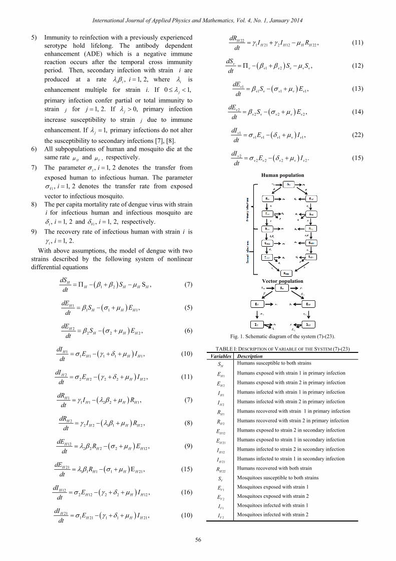
Experiment 1: Infection dies out both strain i and stain j

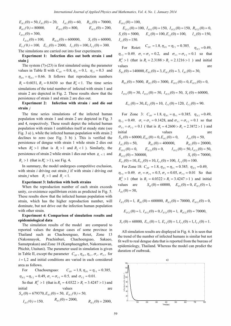
The system (7)-(23) is first simulated using the parameter values in Table II with 10.8, 0.1,HV vC = =η 2 0.3v =η and

1 2 0.66.H H= =η η It follows that reproduction numbers

1 20.6031, 0.8430R R= = so that 0 1.sR < The time series simulations of the total number of infected with strain 1 and strain 2 are depicted in Fig. 2. These results show that the persistence of strain 1 and strain 2 are dies out.

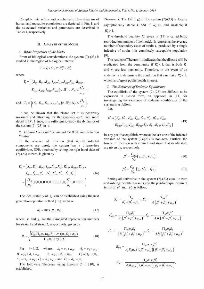
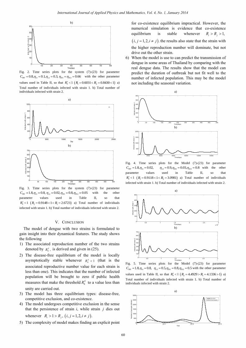
Experiment 2: Infection with strain i and die out strain j

The time series simulations of the infected human population with strain 1 and strain 2 are depicted in Fig. 3 and 4, respectively. These result depict the infected human population with strain 1 establishes itself at steady state (see Fig. 3 a) ), while the infected human population with strain 2 declines to zero (see Fig. 3 b) ). This is verified the persistence of dengue with strain 1 while strain 2 dies out when 0 1sR > (that is 1 1R > and 2 1R < ). Similarly, the persistence of strain 2 while strain 1 dies out when

1 1R < and

2 1R > (that is 0 1sR > ), see Fig. 4. In summary, the model undergoes competitive exclusion,

with strain i driving out strain j if with strain i driving out strain j when 1iR > and 1.jR <

Experiment 3: Infection with both strains When the reproduction number of each strain exceeds

unity, co-existence equilibrium exists as predicted in Fig. 5. These results show that the infected human population with strain, which has the higher reproduction number, will dominate, but not drive out the infection human population with other strain.

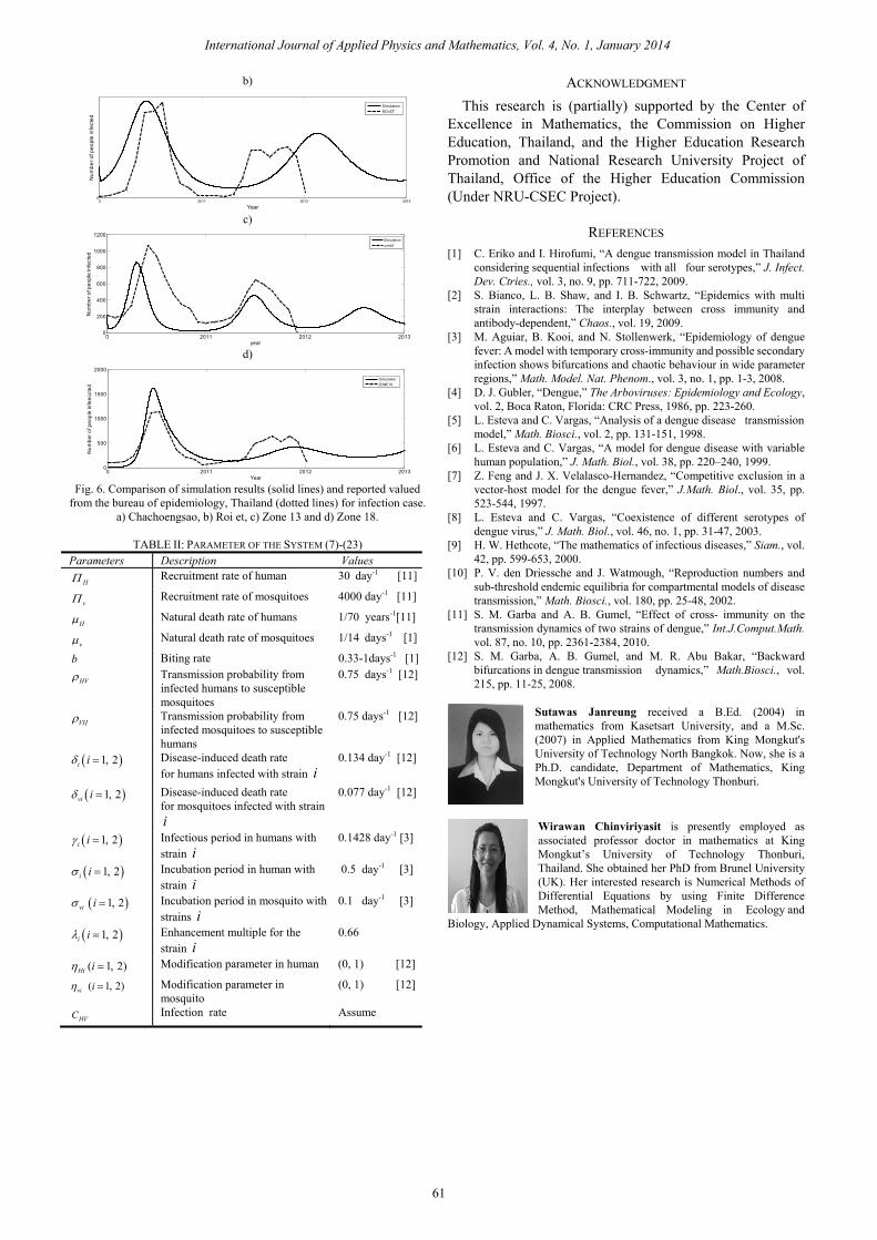
Experiment 4: Comparison of simulation results and epidemiological data

The simulation results of the model are compared to reported values the dengue cases of some province in Thailand such as Chachoengsao, Roiet, Zone 13 (Nakonnayok, Prachinburi, Chachoengsao, Sakaeo, Samutprakan) and Zone 18 (Kamphaengphet, Nakornsawan, Phichit, Utaitani). The parameter used in simulation is given in Table II, except the parameter , , ,HV Hi ViC η η , ,i Viσ σ for

1,2i = and initial conditions are varied in each considered area as follows.

For Chachoengsao: 1 11 8 0 385HV H VC . , . ,= = =η η

2 2 0.49,H V= =η η 1 1 0 5V . ,= =σ σ and 2 0.01.V =σ

So that 1SoR > (that is 2 14 0322 3 4247 1R . R .= > = > ) and

initial values are 1(0) 679370, (0) 50,H HS E= = 2 50 0HE ( ) ,=

1 0 150HI ( ) ,= 1(0) 2000,HR =2 (0) 2000,HR =

12 (0) 001 ,HE =

21(0) 001 ,HE = 12 (0) 150,HI = 21(0) 150,HI = 22 (0) 0,HR =(0) 5000,vS = 1 20(0) 10 , ) 1 ,0(0 0v vE E= = 1(0) 150,vI =

2 (0) 150.vI =

For Roiet: 1 11 8 0 385HV H VC . , . ,= = =η η2 0.49,H =η

2 0 49V . ,=η 1 2 0.2,= =σ σ and 1 2 0.1V V= =σ σ so that

1SoR > (that is 1 22.3188 2.1216 1R R= > = > ) and initial

values are 1 1 2(0) 140000, ( 30) , (0) 3,H H HS E E= = = 1(0) 30,HI =

1(0) 5000,HR = 2 (0) 3000,HR = 12 210(0) , (0) 0,H HE E= =

12 (0) 30,HI = 21(0) 50,HI = 21(0) 50,HI = (0) 60000,VS =

1 20(0) 3 , 10(0) ,V VE E= = 1(0) 120,VI = 2 (0) 90.VI =

For Zone 3: 1 11 8 0 385HV H VC . , . ,= = =η η 2 0.49,H =η

2 0 49V . ,=η 1 2 0.1428,= =σ σ and 1 2 0.1V V= =σ σ so that

1 2 0.1V V= =σ σ ( that is 1 24 2600 2 3872 1R . R .= > = > ) and initial values are

1 2(0) 60000, ( 00) , (0) ,0H H HS E E= = = 1(0) 50,HI =

2 (0) 50,HI = 1(0) 400000,HR = 2 (0) 20000,HR =

12 (0 ,0)HE = 21(0 ,0)HE = 12 21(0) 50, (0) 50,H HI I= =

22 (0) 300000,HR = (0) 70000,VS =

1 2 1(0) 1 , (0) 10 0, (0) 100,V V VE E I= = = 2 (0) 100.VI = For Zone 18: 1 11 8 0 385HV H VC . , . ,= = =η η 2 0.49,H =η

2 0 49V . ,=η 1 1 2 20.5, 0.05, 0.01V V= = = =σ σ σ σ So that 1S

oR > (that is 2 14.0322 3.4247 1R R= > = > ) and initial values are (0) 60000,HS = 1 20(0) , (0) 1,H HE E= =

1(0) 50,HI =

2 (0) 1,HI = 1(0) 600000,HR = 2 (0) 70000,HR = 12 (0 ,0)HE =

21(0) 1,HE = 12 21(0) 0, (0) 1,H HI I= = 22 (0) 70000,HR =

(0) 60000,VS = 1(0) 1,VE = 2 1 2(0) 1, (0) 1, (0) 1.V V VE I I= = =

All simulation results are displayed in Fig. 6. It is seen that the trend of the number of infected humans is similar but not fit well to real dengue data that is reported from the bureau of epidemiology, Thailand. Whereas the model can predict the duration of outbreak.

a)

100 200 300 400 500 600 700 8000

20

40

60

80

100

120

140

160

Time(days)

Infe

cted

with

stra

in 1


59

b)

100 200 300 400 500 600 700 8000

100

200

300

400

500

600

Time(days)

Infe

cted

with

stra

in 2

a)

0 5000 10000 15000 20000 250000

200

400

600

800

1000

Day

Infe

cted

with

stra

in 1

(A)

b)

50 100 150 200 250 300 350 400 450 5000

100

200

300

400

500

600

700

Time(days)

Infe

cted

with

stra

in 2

V. CONCLUSION The model of dengue with two strains is formulated to

gain insight into their dynamical features. The study shows the following 1) The associated reproduction number of the two strains

denoted by 0 ,SR is derived and given in (25). 2) The disease-free equilibrium of the model is locally

asymptotically stable whenever 0 1SR < (that is the associated reproductive number value for each strain is less than one). This indicates that the number of infected population will be brought to zero if public health measures that make the threshold 0

SR to a value less than unity are carried out.

3) The model has three equilibrium types: disease-free, competitive exclusion, and co-existence.

4) The model undergoes competitive exclusion in the sense that the persistence of strain ,i while strain j dies out

whenever 1 ,i jR R> > ( ), 1,2, .i j i j= ≠ 5) The complexity of model makes finding an explicit point

for co-existence equilibrium impractical. However, the numerical simulation is evidence that co-existence equilibrium is stable whenever 1,i jR R> >

( ), 1, 2, .i j i j= ≠ the results also state that the strain with the higher reproduction number will dominate, but not drive out the other strain.

6) When the model is use to can predict the transmission of dengue in some areas of Thailand by comparing with the real dengue data. The results show that the model can predict the duration of outbreak but not fit well to the number of infected population. This may be the model not including the seasonal variation.

a)

0 50 100 150 200 250 300 350 400 450 5000

100

200

300

400

500

600

Time(days)

Infe

cted

with

stra

in 1

b)

4000 6000 8000 10000 12000 140000

500

1000

1500

2000

Time(days)

Infe

cted

with

stra

in 2

a)

0.5 1 1.5 2 2.5 3x 104

0

100

200

300

400

500

Time(days)

Infe

cted

with

stra

in 1

b)

0.5 1 1.5 2 2.5 34

0

100

200

300

400

500

600

700

Time(days)

Infe

cted

with

stra

in 2

a)

0 2011 2012 20130

500

1000

1500

2000

2500

3000

Year

Num

ber o

f peo

ople

infe

cted

SimulationChachoengsao


60

Fig. 2. Time series plots for the system (7)-(23) for parameter

1 2 1 20.8, 0.1, 0.3, 0.66HV v v H HC with the other parameter

values used in Table II, so that 0 1sR 1 20.6031 0.8430 1R R a)

Total number of individuals infected with strain 1. b) Total number of

individuals infected with strain 2.

Fig. 3. Time series plots for the system (7)-(23) for parameter

1 2 1 21.8, 0.8, 0.02, 0.8, 0.05HV v v H HC with the other

parameter values used in Table II, so that

0 1sR 2 10.9148 1 2.6723R R a) Total number of individuals

infected with strain 1. b) Total number of individuals infected with strain 2.

Fig. 4. Time series plots for the Model (7)-(23) for parameter

11.8, 0.02,HV vC 2 1 20.9, 0.03, 0.8v H H with the other

parameter values used in Table II, so that

0 1sR 1 20.9118 1 3.0981R R a) Total number of individuals

infected with strain 1. b) Total number of individuals infected with strain 2.

Fig. 5. Time series plots for the Model (7)-(23) for parameter

11.8, 0.8,HV vC 2 1 20.5, 0.8, 0.5v H H with the other parameter

values used in Table II, so that 0 1sR 2 14.4929 4.1336 1R R a)

Total number of individuals infected with strain 1. b) Total number of

individuals infected with strain 2.

b)

0 2011 2012 20130

Year

Num

ber o

f peo

ple

infe

cted

SimulationROI ET

c)

0 2011 2012 20130

200

400

600

800

1000

1200

year

Num

ber o

f peo

ple

infe

cted

Simulationzone3

d)

0 2011 2012 20130

500

1000

1500

2000

Year

Num

ber o

f peo

ple

infe

ecct

ed

SimulationZONE18

Fig. 6. Comparison of simulation results (solid lines) and reported valued

from the bureau of epidemiology, Thailand (dotted lines) for infection case. a) Chachoengsao, b) Roi et, c) Zone 13 and d) Zone 18.

TABLE II: PARAMETER OF THE SYSTEM (7)-(23)

Parameters Description Values

HΠ Recruitment rate of human 30 day-1 [11]

vΠ Recruitment rate of mosquitoes 4000 day-1 [11]

Hμ Natural death rate of humans 1/70 years-1[11]

vμ Natural death rate of mosquitoes 1/14 days-1 [1]

b Biting rate 0.33-1days-1 [1]

HVρ Transmission probability from infected humans to susceptible mosquitoes

0.75 days-1 [12]

VHρ Transmission probability from infected mosquitoes to susceptible humans

0.75 days-1 [12]

( )1, 2i iδ =

Disease-induced death rate for humans infected with strain i

0.134 day-1 [12]

( )1, 2vi iδ = Disease-induced death rate for mosquitoes infected with strain i

0.077 day-1 [12]

( )1, 2i iγ = Infectious period in humans with strain i

0.1428 day-1 [3]

( )1, 2i iσ = Incubation period in human with strain i

0.5 day-1 [3]

( )1, 2vi iσ = Incubation period in mosquito with strains i

0.1 day-1 [3]

( )1, 2i iλ = Enhancement multiple for the strain i

0.66

( 1, 2)Hi iη = Modification parameter in human (0, 1) [12]

( 1, 2)vi iη = Modification parameter in mosquito

(0, 1) [12]

HVC Infection rate Assume

ACKNOWLEDGMENT This research is (partially) supported by the Center of

Excellence in Mathematics, the Commission on Higher Education, Thailand, and the Higher Education Research Promotion and National Research University Project of Thailand, Office of the Higher Education Commission (Under NRU-CSEC Project).

REFERENCES [1] C. Eriko and I. Hirofumi, “A dengue transmission model in Thailand

considering sequential infections with all four serotypes,” J. Infect. Dev. Ctries., vol. 3, no. 9, pp. 711-722, 2009.

[2] S. Bianco, L. B. Shaw, and I. B. Schwartz, “Epidemics with multi strain interactions: The interplay between cross immunity and antibody-dependent,” Chaos., vol. 19, 2009.

[3] M. Aguiar, B. Kooi, and N. Stollenwerk, “Epidemiology of dengue fever: A model with temporary cross-immunity and possible secondary infection shows bifurcations and chaotic behaviour in wide parameter regions,” Math. Model. Nat. Phenom., vol. 3, no. 1, pp. 1-3, 2008.

[4] D. J. Gubler, “Dengue,” The Arboviruses: Epidemiology and Ecology, vol. 2, Boca Raton, Florida: CRC Press, 1986, pp. 223-260.

[5] L. Esteva and C. Vargas, “Analysis of a dengue disease transmission model,” Math. Biosci., vol. 2, pp. 131-151, 1998.

[6] L. Esteva and C. Vargas, “A model for dengue disease with variable human population,” J. Math. Biol., vol. 38, pp. 220–240, 1999.

[7] Z. Feng and J. X. Velalasco-Hernandez, “Competitive exclusion in a vector-host model for the dengue fever,” J.Math. Biol., vol. 35, pp. 523-544, 1997.

[8] L. Esteva and C. Vargas, “Coexistence of different serotypes of dengue virus,” J. Math. Biol., vol. 46, no. 1, pp. 31-47, 2003.

[9] H. W. Hethcote, “The mathematics of infectious diseases,” Siam., vol. 42, pp. 599-653, 2000.

[10] P. V. den Driessche and J. Watmough, “Reproduction numbers and sub-threshold endemic equilibria for compartmental models of disease transmission,” Math. Biosci., vol. 180, pp. 25-48, 2002.

[11] S. M. Garba and A. B. Gumel, “Effect of cross- immunity on the transmission dynamics of two strains of dengue,” Int.J.Comput.Math. vol. 87, no. 10, pp. 2361-2384, 2010.

[12] S. M. Garba, A. B. Gumel, and M. R. Abu Bakar, “Backward bifurcations in dengue transmission dynamics,” Math.Biosci., vol. 215, pp. 11-25, 2008.

Sutawas Janreung received a B.Ed. (2004) in mathematics from Kasetsart University, and a M.Sc. (2007) in Applied Mathematics from King Mongkut's University of Technology North Bangkok. Now, she is a Ph.D. candidate, Department of Mathematics, King Mongkut's University of Technology Thonburi.

Wirawan Chinviriyasit is presently employed as associated professor doctor in mathematics at King Mongkut’s University of Technology Thonburi, Thailand. She obtained her PhD from Brunel University (UK). Her interested research is Numerical Methods of Differential Equations by using Finite Difference Method, Mathematical Modeling in Ecology and

Biology, Applied Dynamical Systems, Computational Mathematics.


61

Documents

Dengue Fever with Two Strains in Thailand