Dendritic trafficking faces physiologically critical speed ... · 5Division of Biological Sciences, ... 73 Transport along microtubules is mediated by kinesin and dynein motors,

Dendritic trafficking faces physiologically critical1

speed-precision tradeoffs2

Alex H. Williams1,2,3,*, Cian O’Donnell2,4, Terrence Sejnowski2,5, and Timothy O’Leary6,7,*3

1Department of Neurosciences, University of California, San Diego, La Jolla, CA 92093, USA4

2Howard Hughes Medical Institute, Salk Institute for Biological Studies, La Jolla, CA 92037, USA5

3Department of Neurobiology, Stanford University, Stanford, CA 94305, USA6

4Department of Computer Science, University of Bristol, Woodland Road, Bristol, BS8 1UB, United Kingdom7

5Division of Biological Sciences, University of California at San Diego, La Jolla, CA 92093, USA8

6Volen Center and Biology Department, Brandeis University, Waltham, MA 02454, USA9

7Department of Engineering, University of Cambridge, Trumpington St, Cambridge, CB2 1PZ, United Kingdom10

*Address correspondence to: [email protected], [email protected]

ABSTRACT12

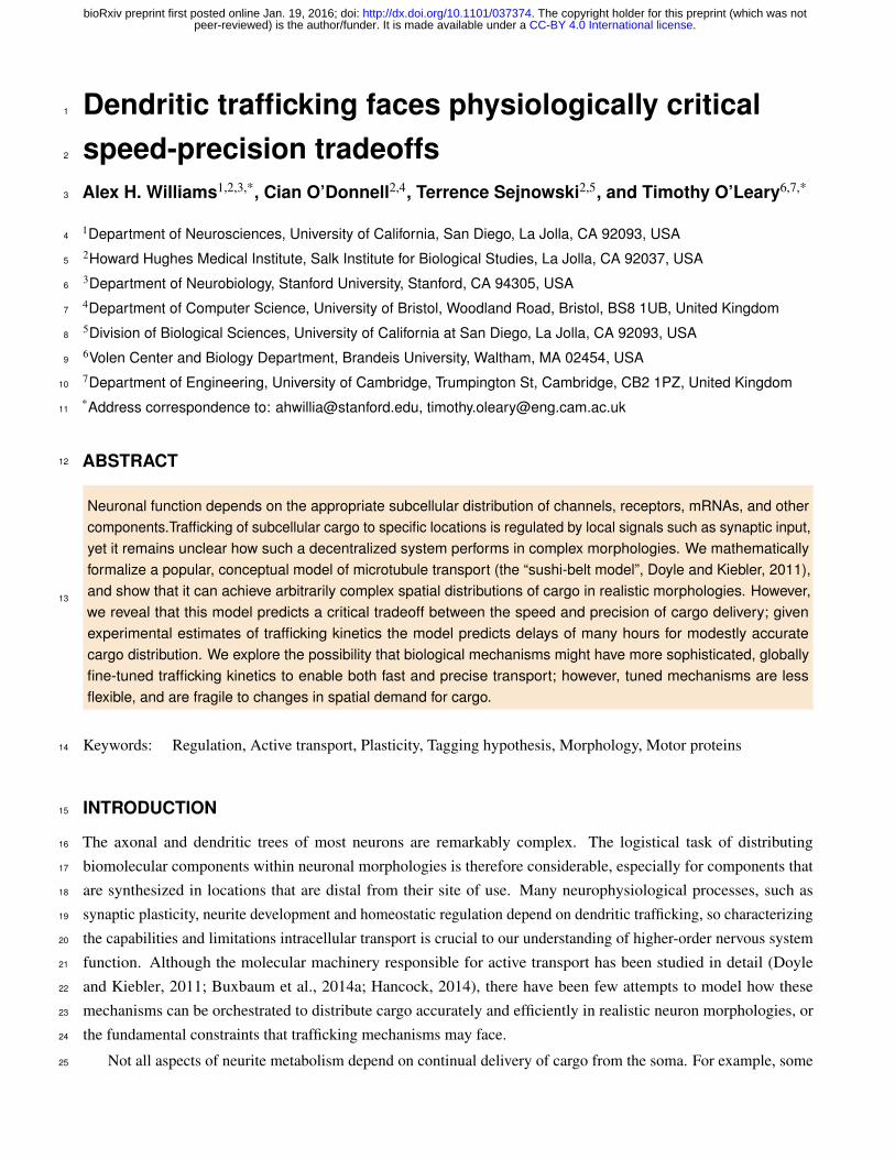
Neuronal function depends on the appropriate subcellular distribution of channels, receptors, mRNAs, and othercomponents.Trafficking of subcellular cargo to specific locations is regulated by local signals such as synaptic input,yet it remains unclear how such a decentralized system performs in complex morphologies. We mathematicallyformalize a popular, conceptual model of microtubule transport (the “sushi-belt model”, Doyle and Kiebler, 2011),and show that it can achieve arbitrarily complex spatial distributions of cargo in realistic morphologies. However,we reveal that this model predicts a critical tradeoff between the speed and precision of cargo delivery; givenexperimental estimates of trafficking kinetics the model predicts delays of many hours for modestly accuratecargo distribution. We explore the possibility that biological mechanisms might have more sophisticated, globallyfine-tuned trafficking kinetics to enable both fast and precise transport; however, tuned mechanisms are lessflexible, and are fragile to changes in spatial demand for cargo.

13

Keywords: Regulation, Active transport, Plasticity, Tagging hypothesis, Morphology, Motor proteins14

INTRODUCTION15

The axonal and dendritic trees of most neurons are remarkably complex. The logistical task of distributing16

biomolecular components within neuronal morphologies is therefore considerable, especially for components that17

are synthesized in locations that are distal from their site of use. Many neurophysiological processes, such as18

synaptic plasticity, neurite development and homeostatic regulation depend on dendritic trafficking, so characterizing19

the capabilities and limitations intracellular transport is crucial to our understanding of higher-order nervous system20

function. Although the molecular machinery responsible for active transport has been studied in detail (Doyle21

and Kiebler, 2011; Buxbaum et al., 2014a; Hancock, 2014), there have been few attempts to model how these22

mechanisms can be orchestrated to distribute cargo accurately and efficiently in realistic neuron morphologies, or23

the fundamental constraints that trafficking mechanisms may face.24

Not all aspects of neurite metabolism depend on continual delivery of cargo from the soma. For example, some25

.CC-BY 4.0 International licensepeer-reviewed) is the author/funder. It is made available under aThe copyright holder for this preprint (which was not. http://dx.doi.org/10.1101/037374doi: bioRxiv preprint first posted online Jan. 19, 2016;

http://dx.doi.org/10.1101/037374

http://creativecommons.org/licenses/by/4.0/

forms of long-term potentiation (LTP) use local protein synthesis and can function in isolated dendrites (Kang and26

Schuman, 1996; Aakalu et al., 2001; Vickers et al., 2005; Sutton and Schuman, 2006; Holt and Schuman, 2013).27

Similarly, constitutive maintenance of cytoskeletal, membrane and signaling pathways is achieved in part by locally28

recycling or synthesizing components (Park et al., 2004, 2006; Grant and Donaldson, 2009; Zheng et al., 2015).29

Nonetheless, components originating in the soma need to find their way to synapses and dendritic branches in the30

first place, and in the long run, the mRNAs and the machinery that supports local biosynthesis need to be replenished.31

More crucially, many long-lasting forms of synaptic plasticity are known to depend on anterograde transport of32

mRNAs (Nguyen et al., 1994; Bading, 2000; Kandel, 2001) and specific mRNAs are known to be selectively33

transported to regions of heightened synaptic activity (Steward et al., 1998; Steward and Worley, 2001; Moga et al.,34

2004) or to developing synaptic contacts (Lyles et al., 2006). These observations fit with the well-known synaptic35

tagging hypothesis (Frey and Morris, 1997, 1998; Redondo and Morris, 2011), which proposes that synapses produce36

a biochemical tag that signals a requirement for synaptic building blocks as part of the plasticity process.37

These neurophysiological functions rely on a number of second-messenger pathways that can also regulate38

the transport and recruitment of intracellular cargo (Doyle and Kiebler, 2011). Kinesin and dyenin motor proteins39

transport cargo along microtubules in a stochastic and bidirectional manner (Block et al., 1990; Smith and Simmons,40

2001; Hirokawa et al., 2010; Gagnon and Mowry, 2011; Park et al., 2014). The stochastic nature of single-particle41

movements has led to the hypothesis that cargo are predominantly controlled by noisy, localized signaling pathways,42

rather than a centralized addressing system (Welte, 2004; Bressloff and Newby, 2009; Newby and Bressloff, 2010;43

Doyle and Kiebler, 2011; Buxbaum et al., 2015). These localized mechanisms are not fully understood, but44

are believed to involve transient elevations in second-messengers like [Ca2+] and ADP (Mironov, 2007; Wang45

and Schwarz, 2009), glutamate receptor activation (Kao et al., 2010; Buxbaum et al., 2014a), and changes in46

microtubule-associated proteins (Soundararajan and Bullock, 2014).47

Based on these observations, several reviews have advanced a conceptual model in which cargo searches the48

dendritic arbor via a noisy walk before its eventual release or capture (Welte, 2004; Buxbaum et al., 2014a, 2015).49

Doyle and Kiebler (2011) refer to this as the “sushi belt model”. In this analogy, molecular cargoes are represented50

by sushi plates that are distributed on a conveyor belt, as found in certain restaurants. Customers sitting alongside51

the belt (representing specific locations or synapses along a dendrite) each have specific and potentially time-critical52

demands for the amount and type of sushi they consume, but they can only choose from nearby plates as they pass.53

Stated in words, the sushi belt model is intuitively plausible, yet a number of open questions remain. For54

example, how can a trafficking system based on local signals be tuned to accurately generate spatial distributions of55

cargo? Does the model predict cross-talk, or interference between spatially separated regions of the neuron that56

require the same kind of cargo? Within this family of models, are there multiple sets of trafficking parameters57

capable of producing the same distribution of cargo, and do they use qualitatively different strategies to produce it?58

Finally, how quickly and how accurately can cargo be delivered by this class of models, and do these measures of59

performance depend on morphology and the specific spatial pattern of demand?60

Each of these high-level questions can be addressed in a parsimonious mathematical framework that is broadly61

applicable to many biological contexts and does not rely on stringent parameter estimates. Here, we present a simple,62

plausible formulation of the sushi belt model that reveals unanticipated features of intracellular trafficking. We63

show that this model can reliably produce complex spatial distributions of cargo across dendritic trees using local64

signals. However, we also reveal strong logistical constraints on this family of models. In particular, we show that65

2/25


http://dx.doi.org/10.1101/037374


fast cargo delivery is error-prone, resulting in cargo distributions that do not match demand. Conversely, modestly66

precise cargo delivery requires many hours based on conservative estimates of trafficking kinetics. We present novel67

models that circumvent this speed-precision tradeoff. However, these possibilities pay a price of greater complexity68

and sensitivity to perturbations. Overall, these predictions suggest new experiments to probe the limitations and69

vulnerabilities of intracellular trafficking, and determine if more complex models beyond the sushi belt are required.70

RESULTS71

Model description72

Transport along microtubules is mediated by kinesin and dynein motors, which are responsible for anterograde and73

retrograde transport, respectively (Hirokawa et al., 2010; Gagnon and Mowry, 2011). Cargo is often simultaneously74

bound to both forms of motor protein, resulting in stochastic back-and-forth movements with a net direction75

determined by the balance of opposing movements (Welte, 2004; Hancock, 2014; Buxbaum et al., 2014a, Fig. 1A).76

To obtain a general model that can accommodate variations in the biophysical details, we interpreted microtubule-77

based transport as a biased random walk along a one-dimensional cable, corresponding to a section of neurite78

(Bressloff, 2006; Bressloff and Newby, 2009; Newby and Bressloff, 2010; Bressloff and Newby, 2013). For each79

time step (1 s), the cargo moves 1 µm forwards, 1 µm backwards, or remains in the same place, each with different80

probabilities. These parameters produce a qualitative fit to a more detailed biophysical model (Muller et al., 2008).81

In the simplest model, the probabilities associated with each movement are fixed and independent across each time82

step, with the forward jump more probable than a reverse jump, leading to a biased random walk (Fig. 1B, top83

panel). Existing biophysical models of single-cargo transport include mechanisms for extended unidirectional runs84

(Muller et al., 2008; Hancock, 2014). To account for these runs, we made a second version of the model in which85

the movement probabilities at each time step depend on the previous position of the particle (see Methods); the86

resulting trajectories change direction less frequently, resulting in a larger variance in cargo position over time (Fig.87

1B, bottom panel).88

While the position of individual cargoes is highly stochastic and dependent on the specific sequence of micro-89

scopic steps, the net movement of a population of cargoes (Fig. 1C) is predictable. This is seen in Figure 1D, which90

shows the distribution of 1000 molecules over time with (top panel) and without (bottom panel) unidirectional runs.91

Thus, bulk trafficking of cargo can be modeled as a deterministic process, which we refer to as the “mass-action92

model” of transport. The model discretizes the dendritic tree into small compartments, and describes the transfer of93

cargo between neighboring compartments as reactions with first order kinetics. In a neurite with N compartments,94

the mass-action model is (Fig. 1E):95

u1a1−⇀↽−b1

u2a2−⇀↽−b2

u3a3−⇀↽−b3

...aN−1−−⇀↽−−bN−1

uN (1)

where ui is the amount of cargo in each compartment, and ai and bi respectively denote local rate constants for96

anterograde and retrograde transport. For now, we assume that these rate constants are spatially homogeneous, since97

the stochastic movements of the single-particle simulations do not depend on position. In this case, the mass-action98

model maps onto the well-known drift-diffusion equation (Fig. 1E Smith and Simmons, 2001) that can be used to99

estimate plausible parameter ranges from experimental data. The drift and diffusion coefficients are respectively100

proportional to the rate of change of the mean and variance of the ensemble distribution (see Methods); thus, an101

experimental measurement of these two quantities on a specific stretch of dendrite would provide a local estimate of102

3/25


http://dx.doi.org/10.1101/037374


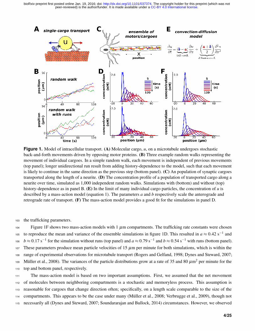
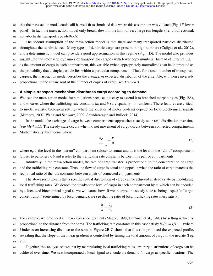
Figure 1. Model of intracellular transport. (A) Molecular cargo, u, on a microtubule undergoes stochasticback-and-forth movements driven by opposing motor proteins. (B) Three example random walks representing themovement of individual cargoes. In a simple random walk, each movement is independent of previous movements(top panel); longer unidirectional run result from adding history-dependence to the model, such that each movementis likely to continue in the same direction as the previous step (bottom panel). (C) An population of synaptic cargoestransported along the length of a neurite. (D) The concentration profile of a population of transported cargo along aneurite over time, simulated as 1,000 independent random walks. Simulations with (bottom) and without (top)history-dependence as in panel B. (E) In the limit of many individual cargo particles, the concentration of u isdescribed by a mass-action model (equation 1). The parameters a and b respectively scale the anterograde andretrograde rate of transport. (F) The mass-action model provides a good fit for the simulations in panel D.

the trafficking parameters.103

Figure 1F shows two mass-action models with 1 µm compartments. The trafficking rate constants were chosen104

to reproduce the mean and variance of the ensemble simulations in figure 1D. This resulted in a ≈ 0.42 s−1 and105

b≈ 0.17 s−1 for the simulation without runs (top panel) and a≈ 0.79 s−1 and b≈ 0.54 s−1 with runs (bottom panel).106

These parameters produce mean particle velocities of 15 µm per minute for both simulations, which is within the107

range of experimental observations for microtubule transport (Rogers and Gelfand, 1998; Dynes and Steward, 2007;108

Muller et al., 2008). The variances of the particle distributions grow at a rate of 35 and 80 µm2 per minute for the109

top and bottom panel, respectively.110

The mass-action model is based on two important assumptions. First, we assumed that the net movement111

of molecules between neighboring compartments is a stochastic and memoryless process. This assumption is112

reasonable for cargoes that change direction often; specifically, on a length scale comparable to the size of the113

compartments. This appears to be the case under many (Muller et al., 2008; Verbrugge et al., 2009), though not114

necessarily all (Dynes and Steward, 2007; Soundararajan and Bullock, 2014) circumstances. However, we observed115

4/25


http://dx.doi.org/10.1101/037374


that the mass-action model could still be well-fit to simulated data where this assumption was violated (Fig. 1F, lower116

panel). In fact, the mass-action model only breaks down in the limit of very large run lengths (i.e. unidirectional,117

non-stochastic transport; see Methods).118

The second assumption of the mass-action model is that there are many transported particles distributed119

throughout the dendritic tree. Many types of dendritic cargo are present in high numbers (Cajigas et al., 2012),120

and a deterministic model can provide a good approximation in this regime (Fig. 1D). The model also provides121

insight into the stochastic dynamics of transport for cargoes with fewer copy numbers. Instead of interpreting u122

as the amount of cargo in each compartment, this variable (when appropriately normalized) can be interpreted as123

the probability that a single particle lies within a particular compartment. Thus, for a small number of transported124

cargoes, the mass-action model describes the average, or expected, distribution of the ensemble, with noise inversely125

proportional to the square root of the number of copies of cargo (see Methods).126

A simple transport mechanism distributes cargo according to demand127

We used the mass-action model for simulations because it is easy to extend it to branched morphologies (Fig. 2A),128

and to cases where the trafficking rate constants (ai and bi) are spatially non-uniform. These features are critical129

to model realistic biological settings where the kinetics of motor proteins depend on local biochemical signals130

(Mironov, 2007; Wang and Schwarz, 2009; Soundararajan and Bullock, 2014).131

In the model, the exchange of cargo between compartments approaches a steady-state (ss), distribution over time132

(see Methods). The steady-state occurs when no net movement of cargo occurs between connected compartments.133

Mathematically, this occurs when:134

up

uc

∣∣∣∣∣ss

=ba

(2)

where up is the level in the “parent” compartment (closer to soma) and uc is the level in the “child” compartment135

(closer to periphery); b and a refer to the trafficking rate constants between this pair of compartments.136

Intuitively, in the mass-action model, the rate of cargo transfer is proportional to the concentration of cargo137

and the trafficking rate constant. Thus, the flow of cargo is equal and opposite when the ratio of cargo matches the138

reciprocal ratio of the rate constants between a pair of connected compartments.139

The above result means that a specific spatial distribution of cargo can be achieved at steady state by modulating140

local trafficking rates. We denote the steady-state level of cargo in each compartment by u, which can be encoded141

by a localized biochemical signal as we will soon show. If we interpret the steady state as being a specific “target142

concentration” (determined by local demand), we see that the ratio of local trafficking rates must satisfy:143

ba=

up

uc(3)

For example, we produced a linear expression gradient (Magee, 1998; Hoffman et al., 1997) by setting u directly144

proportional to the distance from the soma. The trafficking rate constants in this case satisfy bi/ai = i/i+1 (where145

i indexes on increasing distance to the soma). Figure 2B-C shows that this rule produced the expected profile,146

revealing that the slope of the linear gradient is controlled by tuning the total amount of cargo in the neurite (Fig.147

2C).148

Together, this analysis shows that by manipulating local trafficking rates, arbitrary distributions of cargo can be149

achieved over time. We next incorporated a local signal to encode the demand for cargo at specific locations. The150

5/25


http://dx.doi.org/10.1101/037374


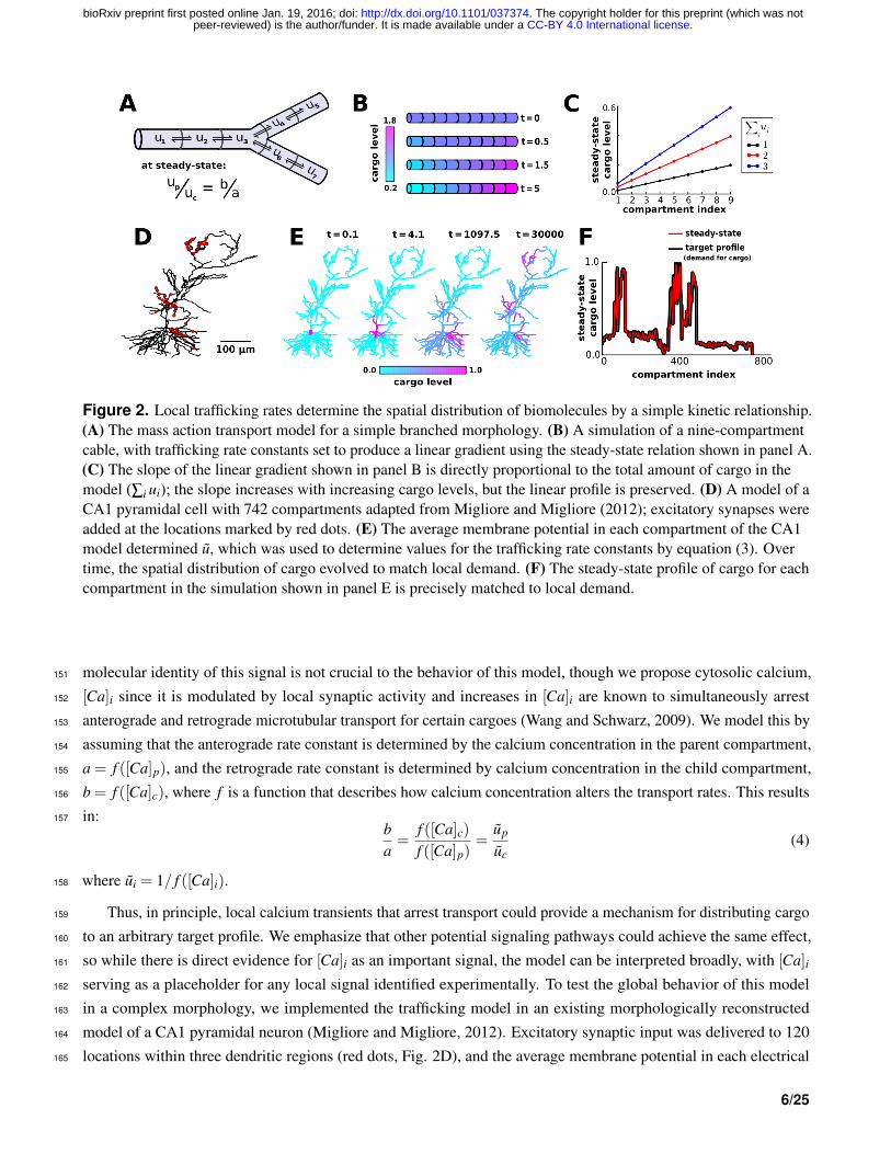
Figure 2. Local trafficking rates determine the spatial distribution of biomolecules by a simple kinetic relationship.(A) The mass action transport model for a simple branched morphology. (B) A simulation of a nine-compartmentcable, with trafficking rate constants set to produce a linear gradient using the steady-state relation shown in panel A.(C) The slope of the linear gradient shown in panel B is directly proportional to the total amount of cargo in themodel (∑i ui); the slope increases with increasing cargo levels, but the linear profile is preserved. (D) A model of aCA1 pyramidal cell with 742 compartments adapted from Migliore and Migliore (2012); excitatory synapses wereadded at the locations marked by red dots. (E) The average membrane potential in each compartment of the CA1model determined u, which was used to determine values for the trafficking rate constants by equation (3). Overtime, the spatial distribution of cargo evolved to match local demand. (F) The steady-state profile of cargo for eachcompartment in the simulation shown in panel E is precisely matched to local demand.

molecular identity of this signal is not crucial to the behavior of this model, though we propose cytosolic calcium,151

[Ca]i since it is modulated by local synaptic activity and increases in [Ca]i are known to simultaneously arrest152

anterograde and retrograde microtubular transport for certain cargoes (Wang and Schwarz, 2009). We model this by153

assuming that the anterograde rate constant is determined by the calcium concentration in the parent compartment,154

a = f ([Ca]p), and the retrograde rate constant is determined by calcium concentration in the child compartment,155

b = f ([Ca]c), where f is a function that describes how calcium concentration alters the transport rates. This results156

in:157ba=

f ([Ca]c)f ([Ca]p)

=up

uc(4)

where ui = 1/ f ([Ca]i).158

Thus, in principle, local calcium transients that arrest transport could provide a mechanism for distributing cargo159

to an arbitrary target profile. We emphasize that other potential signaling pathways could achieve the same effect,160

so while there is direct evidence for [Ca]i as an important signal, the model can be interpreted broadly, with [Ca]i161

serving as a placeholder for any local signal identified experimentally. To test the global behavior of this model162

in a complex morphology, we implemented the trafficking model in an existing morphologically reconstructed163

model of a CA1 pyramidal neuron (Migliore and Migliore, 2012). Excitatory synaptic input was delivered to 120164

locations within three dendritic regions (red dots, Fig. 2D), and the average membrane potential in each electrical165

6/25


http://dx.doi.org/10.1101/037374


compartment determined the target level (ui) in each compartment (Methods). This models how molecular cargo166

could be selectively trafficked to active synaptic sites (Fig. 2E, Supp. Video 1). Figure 2F confirms that the spatial167

distribution of u precisely approaches the desired steady-state exactly in the noise-free case.168

Convergence rate169

Many neurophysiological processes are time-sensitive. For example, newly synthesized proteins must be delivered170

to synapses within ∼1 hour to support long-term potentiation in CA1 pyramidal cells (Frey and Morris, 1997,171

1998; Redondo and Morris, 2011). More generally, biochemical components whose abundance and localization are172

regulated by cellular feedback signals need to be distributed within a time interval that keeps pace with demand,173

within reasonable bounds. We therefore examined how quickly the spatial pattern of cargo converged to its target174

distribution.175

In equations (3) and (4), we implicitly required each ui > 0 in order to avoid division by zero. Intuitively,176

if ui = 0 for some compartment, then no cargo can flow through that compartment, cutting of more peripheral177

compartments from the transport system. Similarly, if certain ui are nearly equal to zero, then transport through178

these compartments will act as a bottleneck for transport, and convergence to the desired distribution will be slow.179

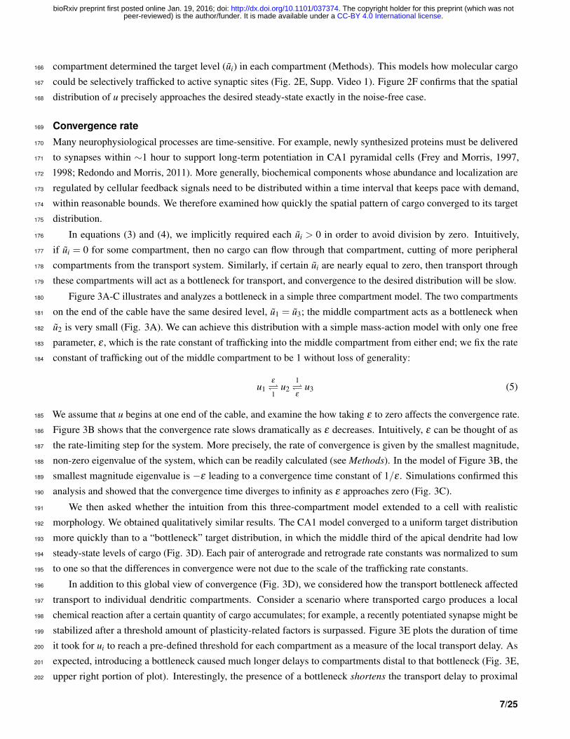
Figure 3A-C illustrates and analyzes a bottleneck in a simple three compartment model. The two compartments180

on the end of the cable have the same desired level, u1 = u3; the middle compartment acts as a bottleneck when181

u2 is very small (Fig. 3A). We can achieve this distribution with a simple mass-action model with only one free182

parameter, ε , which is the rate constant of trafficking into the middle compartment from either end; we fix the rate183

constant of trafficking out of the middle compartment to be 1 without loss of generality:184

u1ε

1

u21ε

u3 (5)

We assume that u begins at one end of the cable, and examine the how taking ε to zero affects the convergence rate.185

Figure 3B shows that the convergence rate slows dramatically as ε decreases. Intuitively, ε can be thought of as186

the rate-limiting step for the system. More precisely, the rate of convergence is given by the smallest magnitude,187

non-zero eigenvalue of the system, which can be readily calculated (see Methods). In the model of Figure 3B, the188

smallest magnitude eigenvalue is −ε leading to a convergence time constant of 1/ε . Simulations confirmed this189

analysis and showed that the convergence time diverges to infinity as ε approaches zero (Fig. 3C).190

We then asked whether the intuition from this three-compartment model extended to a cell with realistic191

morphology. We obtained qualitatively similar results. The CA1 model converged to a uniform target distribution192

more quickly than to a “bottleneck” target distribution, in which the middle third of the apical dendrite had low193

steady-state levels of cargo (Fig. 3D). Each pair of anterograde and retrograde rate constants was normalized to sum194

to one so that the differences in convergence were not due to the scale of the trafficking rate constants.195

In addition to this global view of convergence (Fig. 3D), we considered how the transport bottleneck affected196

transport to individual dendritic compartments. Consider a scenario where transported cargo produces a local197

chemical reaction after a certain quantity of cargo accumulates; for example, a recently potentiated synapse might be198

stabilized after a threshold amount of plasticity-related factors is surpassed. Figure 3E plots the duration of time199

it took for ui to reach a pre-defined threshold for each compartment as a measure of the local transport delay. As200

expected, introducing a bottleneck caused much longer delays to compartments distal to that bottleneck (Fig. 3E,201

upper right portion of plot). Interestingly, the presence of a bottleneck shortens the transport delay to proximal202

7/25


http://dx.doi.org/10.1101/037374


Figure 3. Transport bottlenecks caused by local demand profile. (A) A three-compartment transport model, withthe middle compartment generating a bottleneck. The vertical bars represent the desired steady-state level of cargoin each compartment. The rate of transport into the middle compartment is small (ε , dashed arrows) relative totransport out of the middle compartment. (B) As ε decreases, the model converges more slowly and the steady-statelevel decreases in the middle compartment. (C) Simulations (black dots) confirm that the time to convergence isgiven by the smallest non-zero eigenvalue of the system (analytically calculated line). This eigenvalue can bethought of as the rate-limiting step of the system. (D) Convergence (L1 norm or the sum of absolute value of theresiduals) to a uniform target distribution (red line) is faster than a target distribution containing a bottleneck (blueline) in the CA1 model. (E) For all compartments that reach a threshold level (ui = 0.001), the simulated time ittakes to reach threshold is plotted against the distance of that compartment to the soma. (F) Convergence times forvarious target distributions (str. rad., stratum radiatum; str. lac., stratum lacunosum/moleculare) in the CA1 model.The timescale of all simulations in the CA1 model was set by imposing the constraint that ai +bi = 1 for eachcompartment.

compartments, compared to the uniform target distribution (Fig. 3E, lower left portion of plot). This occurs because203

cargo delayed by the bottleneck spreads throughout the proximal compartments, reaching higher levels earlier in the204

simulation. We observed qualitatively similar results for different local threshold values (data not shown).205

The model predicts that transport to distal compartments will converge to steady-state at a faster rate when206

the steady-state level of cargo in the proximal compartments increases, since this removes a trafficking bottleneck207

between the soma and distal compartments. This can be experimentally tested by characterizing the convergence208

of a macromolecule that aggregates at recently activated synapses, such as Arc mRNA (Steward et al., 1998, see209

Discussion). To illustrate this in the model CA1 cell, we characterized the time course of transport to the distal210

8/25


http://dx.doi.org/10.1101/037374


apical dendrite (stimulating stratum lacunosum/moleculare), proximal apical dendrite (stimulating stratum radiatum),211

entire apical dendrite (stimulating both layers), and entire cell (seizure). Notably, the model converges more slowly212

to distal input alone, than to paired distal and proximal input, or to an entirely uniform input distribution (Fig. 3F).213

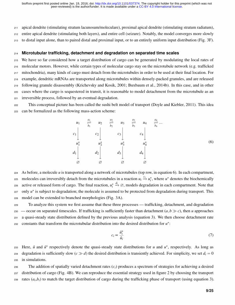
Microtubular trafficking, detachment and degradation on separated time scales214

We have so far considered how a target distribution of cargo can be generated by modulating the local rates of215

molecular motors. However, while certain types of molecular cargo stay on the microtubule network (e.g. trafficked216

mitochondria), many kinds of cargo must detach from the microtubules in order to be used at their final location. For217

example, dendritic mRNAs are transported along microtubules within densely-packed granules, and are released218

following granule disassembly (Krichevsky and Kosik, 2001; Buxbaum et al., 2014b). In this case, and in other219

cases where the cargo is sequestered in transit, it is reasonable to model detachment from the microtubule as an220

irreversible process, followed by an eventual degradation.221

This conceptual picture has been called the sushi belt model of transport (Doyle and Kiebler, 2011). This idea222

can be formalized as the following mass-action scheme:223

u1a1b1

u2a2b2

u3a3b3

u4a4b4

...

c1

y c2

y c3

y c4

yu?1 u?2 u?3 u?4

d1

y d2

y d3

y d4

y∅ ∅ ∅ ∅

(6)

As before, a molecule u is transported along a network of microtubules (top row, in equation 6). In each compartment,224

molecules can irreversibly detach from the microtubules in a reaction uici−→ u?i , where u? denotes the biochemically225

active or released form of cargo. The final reaction, u?idi−→∅, models degradation in each compartment. Note that226

only u? is subject to degradation; the molecule is assumed to be protected from degradation during transport. This227

model can be extended to branched morphologies (Fig. 3A).228

To analyze this system we first assume that these three processes — trafficking, detachment, and degradation229

— occur on separated timescales. If trafficking is sufficiently faster than detachment (a,b� c), then u approaches230

a quasi-steady state distribution defined by the previous analysis (equation 3). We then choose detachment rate231

constants that transform the microtubular distribution into the desired distribution for u?:232

ci ∝u?iui

(7)

Here, u and u? respectively denote the quasi-steady state distributions for u and u?, respectively. As long as233

degradation is sufficiently slow (c� d) the desired distribution is transiently achieved. For simplicity, we set di = 0234

in simulations.235

The addition of spatially varied detachment rates (ci) produces a spectrum of strategies for achieving a desired236

distribution of cargo (Fig. 4B). We can reproduce the essential strategy used in figure 2 by choosing the transport237

rates (ai,bi) to match the target distribution of cargo during the trafficking phase of transport (using equation 3).238

9/25


http://dx.doi.org/10.1101/037374


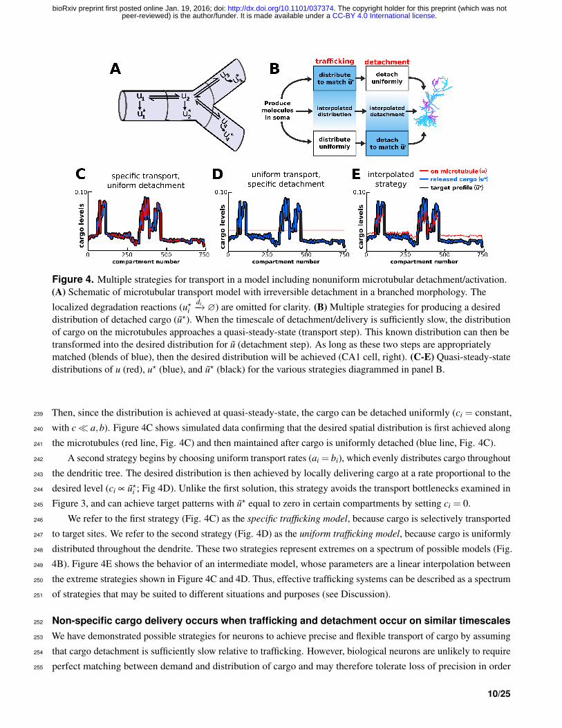
Figure 4. Multiple strategies for transport in a model including nonuniform microtubular detachment/activation.(A) Schematic of microtubular transport model with irreversible detachment in a branched morphology. Thelocalized degradation reactions (u?i

di−→∅) are omitted for clarity. (B) Multiple strategies for producing a desireddistribution of detached cargo (u?). When the timescale of detachment/delivery is sufficiently slow, the distributionof cargo on the microtubules approaches a quasi-steady-state (transport step). This known distribution can then betransformed into the desired distribution for u (detachment step). As long as these two steps are appropriatelymatched (blends of blue), then the desired distribution will be achieved (CA1 cell, right). (C-E) Quasi-steady-statedistributions of u (red), u? (blue), and u? (black) for the various strategies diagrammed in panel B.

Then, since the distribution is achieved at quasi-steady-state, the cargo can be detached uniformly (ci = constant,239

with c� a,b). Figure 4C shows simulated data confirming that the desired spatial distribution is first achieved along240

the microtubules (red line, Fig. 4C) and then maintained after cargo is uniformly detached (blue line, Fig. 4C).241

A second strategy begins by choosing uniform transport rates (ai = bi), which evenly distributes cargo throughout242

the dendritic tree. The desired distribution is then achieved by locally delivering cargo at a rate proportional to the243

desired level (ci ∝ u?i ; Fig 4D). Unlike the first solution, this strategy avoids the transport bottlenecks examined in244

Figure 3, and can achieve target patterns with u? equal to zero in certain compartments by setting ci = 0.245

We refer to the first strategy (Fig. 4C) as the specific trafficking model, because cargo is selectively transported246

to target sites. We refer to the second strategy (Fig. 4D) as the uniform trafficking model, because cargo is uniformly247

distributed throughout the dendrite. These two strategies represent extremes on a spectrum of possible models (Fig.248

4B). Figure 4E shows the behavior of an intermediate model, whose parameters are a linear interpolation between249

the extreme strategies shown in Figure 4C and 4D. Thus, effective trafficking systems can be described as a spectrum250

of strategies that may be suited to different situations and purposes (see Discussion).251

Non-specific cargo delivery occurs when trafficking and detachment occur on similar timescales252

We have demonstrated possible strategies for neurons to achieve precise and flexible transport of cargo by assuming253

that cargo detachment is sufficiently slow relative to trafficking. However, biological neurons are unlikely to require254

perfect matching between demand and distribution of cargo and may therefore tolerate loss of precision in order255

10/25


http://dx.doi.org/10.1101/037374


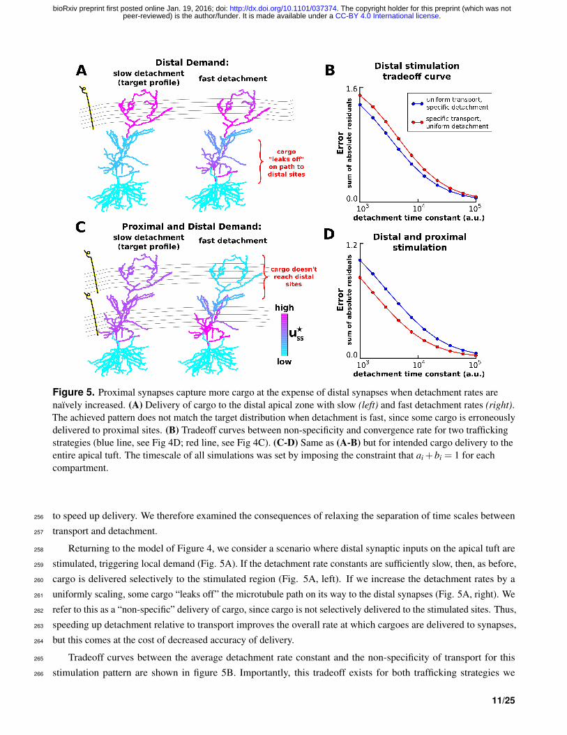
Figure 5. Proximal synapses capture more cargo at the expense of distal synapses when detachment rates arenaıvely increased. (A) Delivery of cargo to the distal apical zone with slow (left) and fast detachment rates (right).The achieved pattern does not match the target distribution when detachment is fast, since some cargo is erroneouslydelivered to proximal sites. (B) Tradeoff curves between non-specificity and convergence rate for two traffickingstrategies (blue line, see Fig 4D; red line, see Fig 4C). (C-D) Same as (A-B) but for intended cargo delivery to theentire apical tuft. The timescale of all simulations was set by imposing the constraint that ai +bi = 1 for eachcompartment.

to speed up delivery. We therefore examined the consequences of relaxing the separation of time scales between256

transport and detachment.257

Returning to the model of Figure 4, we consider a scenario where distal synaptic inputs on the apical tuft are258

stimulated, triggering local demand (Fig. 5A). If the detachment rate constants are sufficiently slow, then, as before,259

cargo is delivered selectively to the stimulated region (Fig. 5A, left). If we increase the detachment rates by a260

uniformly scaling, some cargo “leaks off” the microtubule path on its way to the distal synapses (Fig. 5A, right). We261

refer to this as a “non-specific” delivery of cargo, since cargo is not selectively delivered to the stimulated sites. Thus,262

speeding up detachment relative to transport improves the overall rate at which cargoes are delivered to synapses,263

but this comes at the cost of decreased accuracy of delivery.264

Tradeoff curves between the average detachment rate constant and the non-specificity of transport for this265

stimulation pattern are shown in figure 5B. Importantly, this tradeoff exists for both trafficking strategies we266

11/25


http://dx.doi.org/10.1101/037374


examined in figure 4 — the selective transport strategy (see Fig 4D) and uniform transport strategy (see Fig. 4C).267

For this stimulation pattern, the uniform trafficking strategy (Fig. 5B, blue line) outperforms the specific trafficking268

strategy (Fig. 5B, red line) since the latter suffers from bottleneck in the proximal apical zone.269

The pattern of non-specific delivery is stimulation-dependent. When the entire apical tree is stimulated, fast270

detachment can result in a complete occlusion of cargo delivery to distal synaptic sites (Fig. 5C). As before, a271

tradeoff between specificity and delivery speed is present for both transport strategies (Fig. 5D). Interestingly, the272

specific trafficking strategy outperforms the uniform trafficking strategy in this case (in contrast to Fig. 5A-B). This273

is due to the lack of a bottleneck, and the fact that the uniform trafficking strategy initially sends cargo to the basal274

dendrites where it is not released.275

Together, these results show that an increase in the efficiency of synaptic cargo delivery comes at the cost of276

specificity and that the final destination of mis-trafficked cargo depends on the pattern of stimulation.277

Transport speed and precision can be optimized for specific spatial patterns of demand278

In figure 5, we showed that scaling the detachment rates (ci), while leaving the transport rates (ai, bi) fixed produces279

a proximal bias in cargo delivery. We reasoned that increasing the anterograde transport rate of cargo could correct280

for this bias, producing transport rules that are both fast and precise.281

We examined this possibility in a reduced model — an unbranched cable — so that we could develop simple282

heuristics that precisely achieve a desired distribution of cargo while minimizing the convergence time. In this283

model, cargo begins on the left end of the cable and is transported to a number of synaptic delivery sites, each of284

which is modeled as a double-exponential curve. We also restricted ourselves to investigating the uniform trafficking285

strategy (Fig. 4D); a similar analysis could in principle be done for the specific trafficking strategy.286

As before, cargo can be precisely delivered to a variety of stimulation patterns when the detachment rate is287

sufficiently slow (Fig. 6A, Supp. Video 2); when the detachment rate is naıvely increased to speed up the rate of288

delivery, a proximal bias develops for all stimulation patterns (Fig. 6B, Supp. Video 3).289

We then hand-tuned the transport rate constants to deliver equal cargo to six evenly spaced synaptic sites (top290

row of Fig. 6C, Supp. Video 4). Specifically, we increased the anterograde rate constants (ai) and decreased the291

retrograde rate constants (bi) by a decreasing linear function of position so that aN−1 = bN−1 at the right side of292

the cable. On the left end of the cable, we set a1 = 0.5+β and b1 = 0.5−β , where β is the parameter controlling293

anterograde bias. Intuitively, the profile of the proximal delivery bias is roughly exponential (Fig. 6B, top pattern),294

and therefore the anterograde rates need to be tuned more aggressively near the soma (where the bias is most295

pronounced), and more gently tuned as the distance to the soma increases.296

However, this tuned model does not precisely deliver cargo for other stimulation patterns. For example, when297

the number of synapses on the cable is decreased, a distal delivery bias develops because too little cargo is released298

on the proximal portion of the cable (middle row, Fig. 6C; Supp. Video 5). Even when the number of synapses is299

held constant, changing the position of the synapses can disrupt equitable delivery of cargo to synapses. This is300

shown in the bottom row of figure 6C, where a distal bias again develops after the majority of activated synapses are301

positioned proximally. Thus, within the simple framework we’ve developed, the delivery of cargo can be tuned to302

achieve both precision and speed for a specified target distribution. However, non-specific cargo delivery occurs303

when different stimulation patterns are applied (assuming the transport parameters are not re-tuned).304

12/25


http://dx.doi.org/10.1101/037374


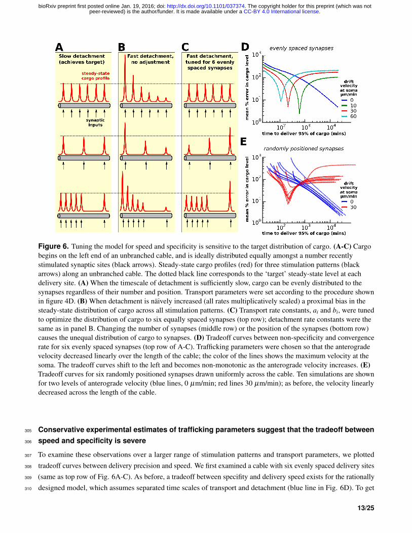
Figure 6. Tuning the model for speed and specificity is sensitive to the target distribution of cargo. (A-C) Cargobegins on the left end of an unbranched cable, and is ideally distributed equally amongst a number recentlystimulated synaptic sites (black arrows). Steady-state cargo profiles (red) for three stimulation patterns (blackarrows) along an unbranched cable. The dotted black line corresponds to the ‘target’ steady-state level at eachdelivery site. (A) When the timescale of detachment is sufficiently slow, cargo can be evenly distributed to thesynapses regardless of their number and position. Transport parameters were set according to the procedure shownin figure 4D. (B) When detachment is naively increased (all rates multiplicatively scaled) a proximal bias in thesteady-state distribution of cargo across all stimulation patterns. (C) Transport rate constants, ai and bi, were tunedto optimize the distribution of cargo to six equally spaced synapses (top row); detachment rate constants were thesame as in panel B. Changing the number of synapses (middle row) or the position of the synapses (bottom row)causes the unequal distribution of cargo to synapses. (D) Tradeoff curves between non-specificity and convergencerate for six evenly spaced synapses (top row of A-C). Trafficking parameters were chosen so that the anterogradevelocity decreased linearly over the length of the cable; the color of the lines shows the maximum velocity at thesoma. The tradeoff curves shift to the left and becomes non-monotonic as the anterograde velocity increases. (E)Tradeoff curves for six randomly positioned synapses drawn uniformly across the cable. Ten simulations are shownfor two levels of anterograde velocity (blue lines, 0 µm/min; red lines 30 µm/min); as before, the velocity linearlydecreased across the length of the cable.

Conservative experimental estimates of trafficking parameters suggest that the tradeoff between305

speed and specificity is severe306

To examine these observations over a larger range of stimulation patterns and transport parameters, we plotted307

tradeoff curves between delivery precision and speed. We first examined a cable with six evenly spaced delivery sites308

(same as top row of Fig. 6A-C). As before, a tradeoff between specifity and delivery speed exists for the rationally309

designed model, which assumes separated time scales of transport and detachment (blue line in Fig. 6D). To get310

13/25


http://dx.doi.org/10.1101/037374


a rough estimate of how severe this tradeoff might be in real neurons, we set the length of the cable to 800 µm311

(roughly the length of an apical dendrite in a CA1 cell) and the diffusion coefficient to 4 µm2/s — an estimate on the312

upper end of what might be biologically achieved (see e.g., Caspi et al., 2000; Soundararajan and Bullock, 2014).313

Despite the optimistic estimate of the diffusion coefficient, the model predicts a severe tradeoff. It takes roughly314

1 day to deliver cargo to match local demand with 10% average error, and roughly a week to deliver within 1%315

average error.316

As the anterograde transport bias is introduced and increased, the optimal points along the tradeoff curve move317

to the left, representing faster transport times. The tradeoff curves also become nonmonotonic: the error (non-318

specificity) initially decreases as the detachment rate decreases, but begins to increase after a certain well-matched319

point. Points on the descending left branch of the curve represent cargo distributions with proximal bias (detachment320

is too fast); points on the ascending right branch correspond to distal bias (detachment is too slow).321

As suggested by the simulations shown in Fig. 6A-C, changing the pattern of cargo demand changes the tradeoff322

curves. Thus, we performed simulations to calculate tradeoff curves for randomizing the number (between 3 and323

9) and position of cargo demand hotspots (Fig. 6E). Notably, the untuned transport model (blue curves) always324

converge to zero error as the detachment rate decreases. In contrast, the model with anterograde bias (red curves)325

exhibit greater variability across demand patterns. Thus, for this model, it appears that the only way to achieve very326

precise, reliable and flexible transport is to have a slow detachment rate.327

DISCUSSION328

We formalized a well-known conceptual model of active transport — the sushi belt model (Doyle and Kiebler,329

2011) — to examine how neurons distribute subcellular cargo subject to biologically realistic trafficking kinetics and330

dendritic morphologies. We found an inherent and surprisingly punishing trade-off between the specificity of cargo331

delivery and the time taken to transport it over realistic dendritic morphologies. In particular, conservative estimates332

based on experimental data predict delays of many hours or even days to match demand within 10%.333

We formulated this model as a simple mass-action system that has a direct biological interpretation and permits334

analysis and simulation. Moreover, the model behaves macroscopically as a drift-diffusion process, providing a335

framework for interpreting and experimentally measuring model parameters (see Methods). From this we developed336

a family of models based on the assumption that sequestration of cargo from a microtubule occurs on a slower337

timescale than trafficking along it. Intuitively, this assumption implies that the cargo has sufficient time to sample338

the dendritic tree for potential delivery sites (Welte, 2004). We showed that the same distribution of cargo could be339

achieved by a family of model parameters ranging from location-dependent trafficking followed by uniform release340

(specific trafficking model) to uniform trafficking followed by location-dependent release (uniform trafficking model).341

Experimental findings appear to span these possibilities, raising the intriguing question of whether transport342

systems might be tuned to suit the needs of specific neuron types, or physiological contexts. Kim and Martin (2015)343

identified three mRNAs that were uniformly distributed in cultured Aplysia sensory neurons, but were targeted to344

synapses at the level of protein expression by localized translation (supporting the uniform trafficking model). In345

contrast, the expression of Arc mRNA is closely matched to the pattern of Arc protein in granule cells of the dentate346

gyrus (Steward et al., 1998; Farris et al., 2014; Steward et al., 2015, supporting the specific trafficking model).347

Trafficking kinetics do not just differ across different cargoes — the same type of molecular cargo can exhibit diverse348

movement statistics in single-particle tracking experiments (Dynes and Steward, 2007). Our work places disparate349

14/25


http://dx.doi.org/10.1101/037374


experimental findings into a common, mathematical framework and shows that the sushi belt model can produce the350

same distribution of cargo with various underlying parameters, supporting its biological plausibility.351

Although the uniform and specific trafficking models can produce the same steady-state distribution of cargo,352

they converge to this distribution at different rates. The specific trafficking model can suffer from bottlenecks353

in the spatial pattern of cargo demand. Furthermore, these bottlenecks can be experimentally induced in cases354

of activity-dependent mRNA transport to test this prediction (see Fig. 3). Due to these bottlenecks, the uniform355

trafficking model often provides faster delivery than the specific trafficking model for a specified accuracy level (but356

see Fig. 5D for a counterexample). This appears to favor the uniform trafficking model from the point of view of357

performance and also due to the fact that uniform trafficking would be easier to implement biologically. However,358

neuronal activity has been observed to influencing trafficking directly (Mironov, 2007; Wang and Schwarz, 2009;359

Soundararajan and Bullock, 2014), and targeted trafficking may have other advantages or functions. For example,360

the non-uniform expression pattern of Arc mRNA could provide a physical substrate to store the spatial pattern of361

synaptic input over long time periods.362

An inherent feature of all versions of the model is a trade-off between the time it takes to deliver cargo to its final363

destination and the accuracy with which its distribution matches the spatial profile of demand. We first asked whether364

the model could maintain precise delivery while relaxing the restriction of slow detachment relative to transport365

along a microtubule. Increasing the rate of detachment produces a proximal bias in the delivery of cargo, leading to a366

mismatch between supply and demand across a population of synapses. Intuitively, a fast detachment rate increases367

the chances for cargo to be delivered prematurely, before it has sampled the dendritic tree for an appropriate delivery368

site. If the transported cargo is involved in synaptic plasticity, this could produce heterosynaptic potentiation (or369

de-potentiation) of proximal synapses when distal synapses are strongly stimulated. Interestingly, this is indeed370

observed in some experimental contexts (Han and Heinemann, 2013). Although we refer to such non-specificity as371

“errors” in cargo delivery, it is possible that heterosynaptic plasticity relationships are leveraged to produce learning372

rules in circuits where synaptic inputs carrying different information sources target spatially distinct regions of the373

dendritic tree (Bittner et al., 2015). Thus, errors and delays might in fact be exploited biologically - especially in374

cases where the underlying mechanism make them inevitable. This cautions against normative assumptions about375

what is optimal biologically and instead emphasizes the importance of general relationships and constraints imposed376

by underlying mechanisms.377

The sushi belt model predicts that the speed-specificity tradeoff is severe across physiologically relevant378

timescales. For accurate cargo delivery, the timescale of cargo dissociation needs to be roughly an order of379

magnitude slower than the timescale of cargo distribution/trafficking. Thus, if it takes roughly 100 minutes to380

distribute cargo throughout the dendrites, it will take roughly 1000 minutes (∼16-17 hours) before the cargo381

dissociates and is delivered to the synapses. This unfavorable scaling may place fundamental limits on what can be382

achieved with nucleus-to-synapse signaling, which is widely thought to be an important mechanism of neuronal383

plasticity (Nguyen et al., 1994; Frey and Morris, 1997, 1998; Bading, 2000; Kandel, 2001; Redondo and Morris,384

2011). Nonetheless, synaptic activity can initiate distal metabolic events including transcription (Kandel, 2001;385

Deisseroth et al., 2003; Greer and Greenberg, 2008; Ch’ng and Martin, 2011). This raises the question of whether386

delays for some kinds of proteins simply do not matter, or are somehow anticipated in downstream regulatory387

pathways. On the other hand, this might also suggest that other mechanisms, such as local translation of sequestered388

mRNA (Holt and Schuman, 2013), are in fact essential for processes that need to avoid nucleus-to-synapse signal389

15/25


http://dx.doi.org/10.1101/037374


delays.390

We then asked whether the speed-specificity tradeoff could be circumvented by globally tuning anterograde391

and retrograde trafficking kinetics as a function of distance from the soma. We were motivated by experimental392

studies which showed that a directional bias in transport can result from changing the proportions of expressed393

motor proteins (Kanai et al., 2004; Amrute-Nayak and Bullock, 2012); such a change might be induced in response394

to synaptic activity (Puthanveettil et al., 2008), or it may be that motor protein expression ratios are tuned during395

development to suit the needs of different neuron types. We were able to tune the transport rates to circumvent396

the speed-specificity tradeoff in an unbranched cable (Fig. 6C, top). However, even when locations for cargo397

demand were uniformly positioned, the trafficking rate constants needed to be tuned non-uniformly along the neurite.398

It is unclear whether real neurons are capable of globally tuning their trafficking rates in a non-uniform manner.399

Simply changing the composition of motor proteins (Amrute-Nayak and Bullock, 2012) is unlikely induce a spatial400

profile in transport bias. On the other hand, non-uniform modulation of the microtubule network or expression401

of microtubule-associated proteins provide potential mechanisms (Kwan et al., 2008; Soundararajan and Bullock,402

2014), but this leaves open the question of how such non-uniform modifications arise to begin with. It would403

therefore be intriguing to experimentally test the existence of spatial gradients in anterograde movement bias, for404

example, using single-particle tracking in living neurons. Furthermore, although tuning transport bias can provide405

fast and rapid cargo delivery for a specific arrangement of synapses along a dendrite, tuned solutions are sensitive406

to changes in densities and spatial distributions of demand, as seen in Figure 6. In addition, the morphology of407

the neurites would affect the tuning, as introducing an anterograde bias naıvely can divert a surplus of cargo into408

proximal branches, resulting in an accumulation of cargo at branch tips (data not shown). Thus, although spatial409

tuning of transport rates can boost trafficking performance, the resulting tuned system may be extremely complex to410

implement and be fragile to perturbations.411

Certain neuron types may nonetheless have morphology and synaptic connectivity that is sufficiently stereotyped412

to allow transport mechanisms to be globally tuned to some degree. In these cases the qualitative prediction that413

anterograde bias should decrease as a function of distance to the soma can be tested experimentally. Such tuning,414

while providing improved efficiency in trafficking intracellular cargo, would also constitute a site of vulnerability415

because alterations in the kinetics of transport or the spatial distribution of demand easily lead to mismatch between416

supply and demand of cargo. Molecular transport is disrupted in a number of neurodegenerative disorders (Tang417

et al., 2012). One obvious consequence of this is that temporal delays in cargo delivery may impair time-sensitive418

physiological processes. Our results highlight a less obvious kind of pathology: due to the broad requirement to419

appropriately match detachment and transport rates in the model, disruption of trafficking speed could additionally420

lead to spatially inaccurate cargo delivery. It would therefore be intriguing to examine whether pathologies caused421

by active transport defects are also associated with aberrant or ectopic localization of important cellular components.422

Conceptual models form the basis of biological understanding, permitting interpretation of experimental data as423

well as motivating new experiments. It is therefore crucial to explore, quantitatively, the behaviour of a conceptual424

model by replacing words with equations. It is possible that active transport in biological neurons will be more robust425

and flexible than the predictions outlined here, which are based on a simple, but widely invoked, conceptual model.426

One noteworthy assumption of this model is that cargo dissociates from the microtubules by a single, irreversible427

reaction. In reality, the capture of cargo may be more complex and involve regulated re-attachment, which might428

prevent synapses from accumulating too much cargo. This possibility, and similar refinements to the sushi belt429

16/25


http://dx.doi.org/10.1101/037374


framework, should be considered as dictated by future experimental results. The minimal models we examined430

provide an essential baseline for future modeling work, since it is difficult to interpret complex models without first431

understanding the features and limitations of their simpler counterparts.432

What further experiments should be done to interrogate the model? A fundamental implication of the model is433

that the timescale of cargo dissociation from the microtubules is critical, as it not only determines the speed of cargo434

delivery, but is also directly related to the accuracy of a un-tuned transport system (Fig. 4) and the flexibility of a435

fine-tuned transport system (Fig. 6). Current experiments have used strong perturbations, such as chemically-induced436

LTP and proteolytic digestion, to induce the rapid release of cargo (Buxbaum et al., 2014a). Experimental tools437

that elicit more subtle effects on cargo dissociation and techniques that accurately measure these effects would438

enable a number of exciting investigations. For example, the sushi belt model predicts that fine-tuned transport439

systems are more sensitive to changes in the cargo dissociation rate. Finding evidence for fine-tuning would identify440

circumstances where neurons require both fast and accurate nucleus-to-synapse communication. In other contexts,441

neurons may tolerate sloppy cargo delivery or even take advantage of it (Han and Heinemann, 2013). Finally, for442

proteins that need to be rapidly, precisely, and flexibly delivered, neurons can sequester and constitutively replenish443

mRNA in the dendrites and rely on localized synthesis to control the spatial expression pattern (Holt and Schuman,444

2013). In all cases, understanding the characteristics of intracellular transport provides clues about the underlying445

mechanisms of the trafficked cargo as well as it’s consequences for higher level physiological functions.446

METHODS447

All simulation code is available online: https://github.com/ahwillia/Williams-etal-Synaptic-Transport448

Model of single-particle transport449

Let xn denote the position of a particle along a 1-dimensional cable at timestep n. Let vn denote the velocity of450

the particle at timestep n; for simplicity, we assume the velocity can take on three discrete values, vn = {−1,0,1},451

corresponding to a retrograde movement, pause, or anterograde movement. As a result, xn is constrained to take on452

integer values. In the memoryless transport model (top plots in Fig. 1B, 1D, and 1F), we assume that vn is drawn453

with fixed probabilities on each step. The update rule for position is:454

xn+1 = xn + vn

455

vn+1 =

−1 with probability p−0 with probability p0

1 with probability p+

We chose p− = 0.2, p0 = 0.35 and p+ = 0.45 for the illustration shown in Figure 1. For the model with456

history-dependence (bottom plots in Fig. 1B, 1D, and 1F), the movement probabilities at each step depend on the457

previous movement. For example, if the motor was moving in an anterograde direction on the previous timestep,458

then it is more likely to continue to moving in that direction in the next time step. In this case the update rule is459

17/25


http://dx.doi.org/10.1101/037374


written in terms of conditional probabilities:460

vn+1 =

−1 with probability p(−|vn)

0 with probability p(0|vn)

1 with probability p(+|vn)

In the limiting (non-stochastic) case of history-dependence, the particle always steps in the same direction as the461

previous time step.462

vn =−1 vn = 0 vn = 1

p(vn+1 =−1) 1 0 0

p(vn+1 = 0) 0 1 0

p(vn+1 = 1) 0 0 1

We introduce a parameter k ∈ [0,1] to linearly interpolate between this extreme case and the memoryless model.463

The bottom plots of figure 1B, 1D were simulated with k = 0.5; in the bottom plot of figure 1F, a mass-action model464

was fit to these simulations.465

Relationship of single-particle transport to the mass-action model466

The mass-action model (equation 1, in the Results) simulates the bulk movement of cargo u across discrete467

compartments. The rate of cargo transfer is modeled as elementary chemical reactions (Keener and Sneyd, 1998).468

For an unbranched cable, the change in cargo in compartment i is given by:469

ui = aui−1 +bui+1− (a+b)ui (8)

For now, we assume that the anterograde and retrograde trafficking rate constants (a and b, respectively) are spatially470

uniform.471

The mass-action model can be related to a drift-diffusion partial differential equation (Fig. 1E Smith and

Simmons, 2001) by discretizing u into spatial compartments of size ∆ and expanding around some position, x:

u(x)≈ a[

u(x)−∆∂u∂x

+∆2

2∂ 2u∂x2

]+b[

u(x)+∆∂u∂x

+∆2

2∂ 2u∂x2

]− (a+b) u(x) (9)

= a[−∆

∂u∂x

+∆2

2∂ 2u∂x2

]+b[

∆∂u∂x

+∆2

2∂ 2u∂x2

](10)

We keep terms to second order in ∆, as these are of order dt in the limit ∆→ 0 (Gardiner, 2009). This leads to a472

drift-diffusion equation:473

u(x) =∂u∂ t

= (b−a)︸︷︷︸drift coefficient

∂u∂x

+

(a+b

2

)︸︷︷︸

diffusion coefficient

∂ 2u∂x2 (11)

Measurements of the mean and mean-squared positions of particles in tracking experiments, or estimates of the474

average drift rate and dispersion rate of a pulse of labeled particles can thus provide estimates of parameters a and b.475

How does this equation relate to the model of single-particle transport (Fig. 1A-B)? For a memoryless biased476

random walk, the expected position of a particle after n time steps is E[xn] = n(p+− p−) and the variance in position477

after n steps is n(

p++ p−− (p+− p−)2). For large numbers of independently moving particles the mean and478

18/25


http://dx.doi.org/10.1101/037374


variance calculations for a single particle can be directly related to the ensemble statistics outlined in the previous479

paragraph. We find:480

a =2p+− (p+− p−)2

2481

b =2p−− (p+− p−)2

2

The above analysis changes slightly when the single-particle trajectories contain long, unidirectional runs. The482

expected position for any particle is the same E[xn] = n(p+− p−); the variance, in contrast, increases as run lengths483

increase. However, the mass-action model can often provide a good fit in this regime with appropriately re-fit484

parameters (see Fig. 1F). As long as the single-particles have stochastic and identically distributed behavior, the485

ensemble will be well-described by a normal distribution by the central limit theorem. This only breaks down in the486

limit of very long unidirectional runs, as the system is no longer stochastic.487

Estimating parameters of the mass-action model using experimental data488

The parameters of the mass-action model we study can be experimentally fit by estimating the drift and diffusion489

coefficients of particles over the length of a neurite. A commonly used approach to this is to plot the mean490

displacement and mean squared displacement of particles as a function of time. The slopes of the best-fit lines491

in these cases respectively estimate the drift and diffusion coefficients in (11). Diffusion might not accurately492

model particle movements over short time scales because unidirectional cargo runs result in superdiffusive motion,493

evidenced by superlinear increases in mean squared-displacement with time (Caspi et al., 2000). However, drift-494

diffusion does appear to be a good model for particle transport over longer time scales with stochastic changes in495

direction (Soundararajan and Bullock, 2014).496

The mass-action model can also be fit by tracking the positions of a population of particles with photoactivatable497

GFP (Roy et al., 2012). In this case, the distribution of fluorescence at each point in time could be fit by Gaussian498

distributions; the drift and diffusion coefficients are respectively proportional to the rate at which the mean and499

variance of this distribution changes.500

These experimental measurements can vary substantially across neuron types, experimental conditions, and501

cargo identities. Therefore, in order to understand fundamental features and constraints of the sushi belt model across502

systems, it is more useful to explore relationships within the model across ranges of parameters. Unless otherwise503

stated, the trafficking kinetics were constrained so that ai +bi = 1 for each pair of connected compartments. This504

is equivalent to having a constant diffusion coefficient of one across all compartments. Given a target expression505

pattern along the microtubules, this is the only free parameter of the trafficking simulations; increasing the diffusion506

coefficient will always shorten convergence times, but not qualitatively change our results. In figures 1 and 6, we507

derived estimates of the trafficking parameters using drift and diffusion coefficients from single-particle tracking508

experiments (Caspi et al., 2000; Soundararajan and Bullock, 2014).509

Steady-state analysis510

The steady-state ratio of trafficked cargo in neighboring compartments equals the ratio of trafficking rate constants511

(equation 2). Consider a unbranched neurite with non-uniform anterograde and retrograde rate constants (equation512

19/25


http://dx.doi.org/10.1101/037374


1). It is easy to verify the steady-state relationship in the first two compartments, by setting u1 = 0 and solving:513

−a1u1 +b1u2 = 0 ⇒ u1

u2

∣∣∣∣∣ss

=b1

a1

Successively applying the same logic down the cable confirms the condition in equation 2 holds globally. The more514

general condition for branched morphologies can be proven by a similar procedure (starting at the tips and moving515

in).516

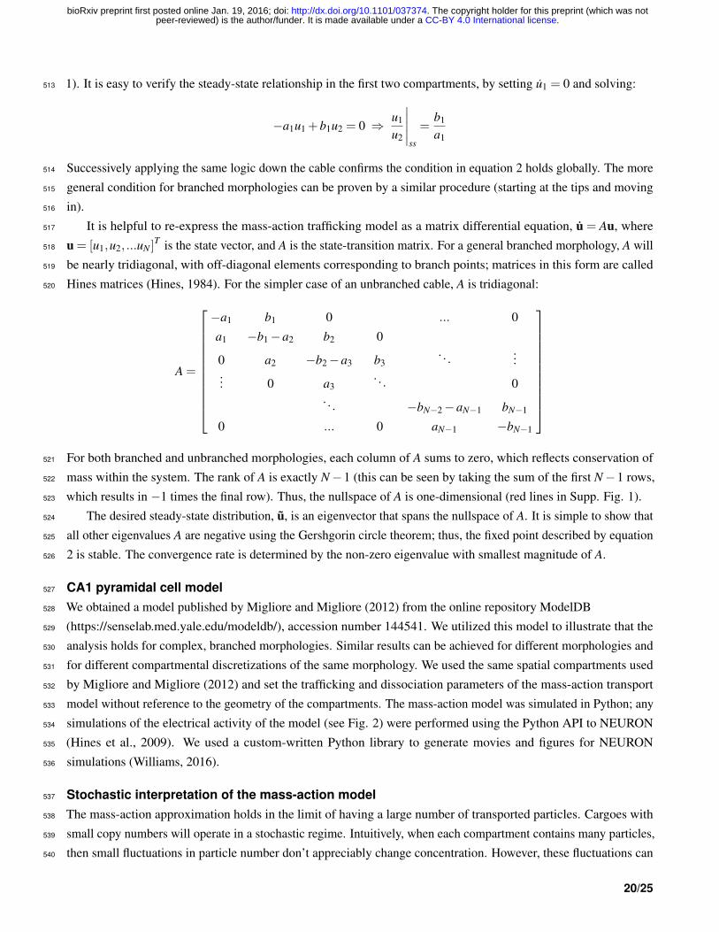
It is helpful to re-express the mass-action trafficking model as a matrix differential equation, u = Au, where517

u = [u1,u2, ...uN ]T is the state vector, and A is the state-transition matrix. For a general branched morphology, A will518

be nearly tridiagonal, with off-diagonal elements corresponding to branch points; matrices in this form are called519

Hines matrices (Hines, 1984). For the simpler case of an unbranched cable, A is tridiagonal:520

A =

−a1 b1 0 ... 0

a1 −b1−a2 b2 0

0 a2 −b2−a3 b3. . .

...... 0 a3

. . . 0. . . −bN−2−aN−1 bN−1

0 ... 0 aN−1 −bN−1

For both branched and unbranched morphologies, each column of A sums to zero, which reflects conservation of521

mass within the system. The rank of A is exactly N−1 (this can be seen by taking the sum of the first N−1 rows,522

which results in −1 times the final row). Thus, the nullspace of A is one-dimensional (red lines in Supp. Fig. 1).523

The desired steady-state distribution, u, is an eigenvector that spans the nullspace of A. It is simple to show that524

all other eigenvalues A are negative using the Gershgorin circle theorem; thus, the fixed point described by equation525

2 is stable. The convergence rate is determined by the non-zero eigenvalue with smallest magnitude of A.526

CA1 pyramidal cell model527

We obtained a model published by Migliore and Migliore (2012) from the online repository ModelDB528

(https://senselab.med.yale.edu/modeldb/), accession number 144541. We utilized this model to illustrate that the529

analysis holds for complex, branched morphologies. Similar results can be achieved for different morphologies and530

for different compartmental discretizations of the same morphology. We used the same spatial compartments used531

by Migliore and Migliore (2012) and set the trafficking and dissociation parameters of the mass-action transport532

model without reference to the geometry of the compartments. The mass-action model was simulated in Python; any533

simulations of the electrical activity of the model (see Fig. 2) were performed using the Python API to NEURON534

(Hines et al., 2009). We used a custom-written Python library to generate movies and figures for NEURON535

simulations (Williams, 2016).536

Stochastic interpretation of the mass-action model537

The mass-action approximation holds in the limit of having a large number of transported particles. Cargoes with538

small copy numbers will operate in a stochastic regime. Intuitively, when each compartment contains many particles,539

then small fluctuations in particle number don’t appreciably change concentration. However, these fluctuations can540

20/25


http://dx.doi.org/10.1101/037374


be functionally significant when the number of particles is small — for example, even a very energetically favorable541

reaction cannot occur with zero particles, but may occur with reasonable probability when a few particles are present.542

We can thus interpret ui as the probability of a particle occupying compartment i at a particular time. This543

invokes a standard technical assumption that the system is ergodic, meaning that position of one particle averaged544

over very long time intervals is the same as the ensemble steady-state distribution.545

Thus, in addition to modeling how the spatial distribution of cargo changes over time, the mass-action model546

equivalently models a spatial probability distribution. That is, imagine we track a single cargo and ask its position547

after a long period of transport. The probability ratio between of finding this particle in any parent-child pair of548

compartments converges to:549

pp

pc

∣∣∣∣ss=

ba

which matches the steady-state analysis of the deterministic model.550

In the stochastic model, the number of molecules in each compartment converges to a binomial distribution at551

steady-state; the coefficient of variation in each compartment is given by:552 √√√√1− p(ss)i

n p(ss)i

This suggests two ways of decreasing noise in the system. First, increasing the total number of transported molecules,553

n, decreases the noise by a factor of 1/√

n. Additionally, transport is more reliable to compartments with a high554

steady-state occupation probability.555

Incorporating detachment and degradation into the mass-action model556

Introducing detachment and degradation reactions into the transport model is straightforward. For an arbitrary557

compartment in a cable, the differential equations become:558

ui = ai−1ui−1− (ai +bi−1 + ci)ui +biui+1

u?i = ciui−diu?i

When ai,bi� ci� di, then the variables ui and u?i approach a quasi-steady-state, which we denote ui and u?i .559

For simplicity we assume di = 0 in simulations. We present two strategies for achieving a desired distribution for560

u?i in figure 4C and 4D. To interpolate between these strategies, let F be a scalar between 0 and 1, and let u? be561

normalized to sum to one. We choose ai and bi to achieve:562

ui = F u?i +(1−F)/N

along the microtubular network and choose ci to satisfy563

ci ∝u?i

F u?i +(1−F)/N

Here, N is the number of compartments in the model. Setting F = 1 results in the simulation in the “specific”564

trafficking model (Fig. 4C), while setting F = 0 results in the “uniform” trafficking model (Fig. 4D). An interpolated565

21/25


http://dx.doi.org/10.1101/037374


strategy is shown in figure 4E (F = 0.3).566

Globally tuning transport rates to circumvent the speed-specificity tradeoff567

We investigated the uniform trafficking model with fast detachment rates in an unbranched cable with equally spaced568

synapses and N = 100 compartments. Multiplicatively increasing the detachment rates across the cable produced a569

proximal bias in cargo delivery which could be corrected by setting the anterograde and retrograde trafficking rates570

to be:571

ai = 0.5+β · N−1− iN−2

572

bi = 0.5−β · N−1− iN−2

where i = {1,2, ...N−1} indexes the trafficking rates from the soma (i = 1) to the other end of the cable (i = N−1).573

Faster detachment rates require larger values for the parameter β ; note that β < 0.5 is a constraint to prevent bi from574

becoming negative. This heuristic qualitatively improved, but did not precisely correct for, fast detachment rates in575

the specific trafficking model (data not shown).576

ACKNOWLEDGEMENTS577

We thank Eve Marder, Subhaneil Lahiri, Friedemann Zenke, and Benjamin Regner for useful feedback on the578

manuscript, and thank Simon Bullock for useful discussion. This research was supported by the Department of579

Energy Computational Science Graduate Fellowship, NIH Grant 1P01NS079419, NIH Grant P41GM103712, the580

Howard Hughes Medical Institute, and the Charles A. King Trust.581

COMPETING INTERESTS582

The authors declare that there are no competing interests.583

REFERENCES584

Aakalu, G., Smith, W. B., Nguyen, N., Jiang, C., and Schuman, E. M. (2001). Dynamic visualization of local protein585

synthesis in hippocampal neurons. Neuron, 30(2):489–502.586

Amrute-Nayak, M. and Bullock, S. L. (2012). Single-molecule assays reveal that RNA localization signals regulate587

dynein-dynactin copy number on individual transcript cargoes. Nat. Cell Biol., 14(4):416–423.588

Bading, H. (2000). Transcription-dependent neuronal plasticity. Eur. J. Biochem., 267(17):5280–5283.589

Bittner, K. C., Grienberger, C., Vaidya, S. P., Milstein, A. D., Macklin, J. J., Suh, J., Tonegawa, S., and Magee, J. C.590

(2015). Conjunctive input processing drives feature selectivity in hippocampal CA1 neurons. Nat. Neurosci.,591

18(8):1133–1142.592

Block, S. M., Goldstein, L. S. B., and Schnapp, B. J. (1990). Bead movement by single kinesin molecules studied593

with optical tweezers. Nature, 348(6299):348–352.594

Bressloff, P. and Newby, J. (2009). Directed intermittent search for hidden targets. New J. Phys., 11(2):023033.595

Bressloff, P. C. (2006). Stochastic model of protein receptor trafficking prior to synaptogenesis. Phys. Rev. E Stat.596

Nonlin. Soft. Matter. Phys., 74(3).597

Bressloff, P. C. and Newby, J. M. (2013). Stochastic models of intracellular transport. Rev. Mod. Phys., 85(1):135–598

196.599

22/25


http://dx.doi.org/10.1101/037374


Buxbaum, A. R., Haimovich, G., and Singer, R. H. (2014a). In the right place at the right time: visualizing and600

understanding mRNA localization. Nat. Rev. Mol. Cell Biol., 16(2):95–109.601

Buxbaum, A. R., Wu, B., and Singer, R. H. (2014b). Single-Actin mRNA Detection in Neurons Reveals a Mechanism602

for Regulating Its Translatability. Science, 343(6169):419–422.603

Buxbaum, A. R., Yoon, Y. J., Singer, R. H., and Park, H. Y. (2015). Single-molecule insights into mRNA dynamics604

in neurons. Trends Cell Biol., 25(8):468–475.605

Cajigas, I. J., Tushev, G., Will, T. J., tom Dieck, S., Fuerst, N., and Schuman, E. M. (2012). The local transcriptome606

in the synaptic neuropil revealed by deep sequencing and high-resolution imaging. Neuron, 74(3):453–466.607

Caspi, A., Granek, R., and Elbaum, M. (2000). Enhanced diffusion in active intracellular transport. Phys. Rev. Lett.,608

85:5655–5658.609

Ch’ng, T. and Martin, K. (2011). Synapse-to-nucleus signaling. Curr. Opin. Neurobiol., 21:345–52.610

Deisseroth, K., Mermelstein, P. G., Xia, H., and Tsien, R. W. (2003). Signaling from synapse to nucleus: the logic611

behind the mechanisms. Curr. Opin. Neurobiol., 13(3):354–365.612

Doyle, M. and Kiebler, M. A. (2011). Mechanisms of dendritic mRNA transport and its role in synaptic tagging.613

EMBO J., 30(17):3540–3552.614

Dynes, J. L. and Steward, O. (2007). Dynamics of bidirectional transport of Arc mRNA in neuronal dendrites. J.615

Comp. Neurol., 500(3):433–447.616

Farris, S., Lewandowski, G., Cox, C. D., and Steward, O. (2014). Selective Localization of Arc mRNA in Dendrites617

Involves Activity- and Translation-Dependent mRNA Degradation. J. Neurosci., 34(13):4481–4493.618

Frey, U. and Morris, R. (1998). Weak before strong: dissociating synaptic tagging and plasticity-factor accounts of619

late-LTP. Neuropharmacol., 37(4-5):545–552.620

Frey, U. and Morris, R. G. M. (1997). Synaptic tagging and long-term potentiation. Nature, 385(6616):533–536.621

Gagnon, J. and Mowry, K. (2011). Molecular motors: directing traffic during RNA localization. Crit Rev Biochem622

Mol Biol, 46:229–39.623

Gardiner, C. (2009). Stochastic Methods: A Handbook for the Natural and Social Sciences (Springer Series in624

Synergetics). Springer, 4 edition.625

Grant, B. D. and Donaldson, J. G. (2009). Pathways and mechanisms of endocytic recycling. Nat. Rev. Mol. Cell626

Biol., 10(9):597–608.627

Greer, P. L. and Greenberg, M. E. (2008). From synapse to nucleus: Calcium-dependent gene transcription in the628

control of synapse development and function. Neuron, 59(6):846 – 860.629

Han, E. B. and Heinemann, S. F. (2013). Distal Dendritic Inputs Control Neuronal Activity by Heterosynaptic630

Potentiation of Proximal Inputs. J. Neurosci., 33(4):1314–1325.631

Hancock, W. O. (2014). Bidirectional cargo transport: moving beyond tug of war. Nat. Rev. Mol. Cell Biol.,632

15(9):615–628.633

Hines, M. (1984). Efficient computation of branched nerve equations. Int. J. Biomed. Comput., 15(1):69–76.634

Hines, M. L., Davison, A. P., and Muller, E. (2009). Neuron and python. Front. Neuroinform., 3.635

Hirokawa, N., Niwa, S., and Tanaka, Y. (2010). Molecular Motors in Neurons: Transport Mechanisms and Roles in636

Brain Function Development, and Disease. Neuron, 68(4):610–638.637

Hoffman, D., Magee, J., Colbert, C., and Johnston, D. (1997). K+ channel regulation of signal propagation in638

dendrites of hippocampal pyramidal neurons. Nature, 387:869–75.639

23/25


http://dx.doi.org/10.1101/037374


Holt, C. E. and Schuman, E. M. (2013). The central dogma decentralized: New perspectives on RNA function and640

local translation in neurons. Neuron, 80(3):648–657.641

Kanai, Y., Dohmae, N., and Hirokawa, N. (2004). Kinesin transports RNA: isolation and characterization of an642

RNA-transporting granule. Neuron, 43(4):513–525.643

Kandel, E. R. (2001). The Molecular Biology of Memory Storage: A Dialogue Between Genes and Synapses.644

Science, 294(5544):1030–1038.645

Kang, H. and Schuman, E. M. (1996). A requirement for local protein synthesis in neurotrophin-induced hippocampal646

synaptic plasticity. Science, 273(5280):1402–1406.647

Kao, D.-I., Aldridge, G. M., Weiler, I. J., and Greenough, W. T. (2010). Altered mrna transport, docking, and protein648

translation in neurons lacking fragile x mental retardation protein. Proc. Natl. Acad. Sci. USA, 107(35):15601–649

15606.650

Keener, J. P. and Sneyd, J. (1998). Mathematical Physiology. Springer, New York.651

Kim, S. and Martin, K. C. (2015). Neuron-wide RNA transport combines with netrin-mediated local translation to652

spatially regulate the synaptic proteome. eLife, 4:e04158.653

Krichevsky, A. M. and Kosik, K. S. (2001). Neuronal RNA GranulesA Link between RNA Localization and654

Stimulation-Dependent Translation. Neuron, 32(4):683–696.655

Kwan, A. C., Dombeck, D. A., and Webb, W. W. (2008). Polarized microtubule arrays in apical dendrites and axons.656

Proc. Natl. Acad. Sci. U.S.A., 105(32):11370–11375.657

Lyles, V., Zhao, Y., and Martin, K. C. (2006). Synapse Formation and mRNA Localization in Cultured Aplysia658

Neurons. Neuron, 49(3):349–356.659

Magee, J. (1998). Dendritic hyperpolarization-activated currents modify the integrative properties of hippocampal660

CA1 pyramidal neurons. J Neurosci, 18:7613–24.661

Migliore, M. and Migliore, R. (2012). Know your current Ih: Interaction with a shunting current explains the662

puzzling effects of its pharmacological or pathological modulations. PLoS ONE, 7(5):e36867.663

Mironov, S. L. (2007). ADP Regulates Movements of Mitochondria in Neurons. Biophys. J., 92(8):2944–2952.664

Moga, D., Calhoun, M., Chowdhury, A., Worley, P., Morrison, J., and Shapiro, M. (2004). Activity-regulated665

cytoskeletal-associated protein is localized to recently activated excitatory synapses. Neurosci., 125(1):7–11.666

Muller, M. J. I., Klumpp, S., and Lipowsky, R. (2008). Tug-of-war as a cooperative mechanism for bidirectional667

cargo transport by molecular motors. Proc. Natl. Acad. Sci. U.S.A., 105(12):4609–4614.668

Newby, J. and Bressloff, P. C. (2010). Local synaptic signaling enhances the stochastic transport of motor-driven669

cargo in neurons. Phys. Biol., 7(3):036004.670

Nguyen, P. V., Abel, T., and Kandel, E. R. (1994). Requirement of a critical period of transcription for induction of a671

late phase of LTP. Science, 265(5175):1104–1107.672

Park, H. Y., Lim, H., Yoon, Y. J., Follenzi, A., Nwokafor, C., Lopez-Jones, M., Meng, X., and Singer, R. H. (2014).673

Visualization of dynamics of single endogenous mRNA labeled in live mouse. Science, 343(6169):422–424.674

Park, M., Penick, E. C., Edwards, J. G., Kauer, J. A., and Ehlers, M. D. (2004). Recycling endosomes supply AMPA675

receptors for LTP. Science, 305(5692):1972–1975.676

Park, M., Salgado, J. M., Ostroff, L., Helton, T. D., Robinson, C. G., Harris, K. M., and Ehlers, M. D. (2006).677

Plasticity-induced growth of dendritic spines by exocytic trafficking from recycling endosomes. Neuron, 52(5):817–678

830.679

24/25


http://dx.doi.org/10.1101/037374


Puthanveettil, S. V., Monje, F. J., Miniaci, M. C., Choi, Y.-B., Karl, K. A., Khandros, E., Gawinowicz, M. A.,680

Sheetz, M. P., and Kandel, E. R. (2008). A New Component in Synaptic Plasticity: Upregulation of Kinesin in the681

Neurons of the Gill-Withdrawal Reflex. Cell, 135(5):960–973.682

Redondo, R. L. and Morris, R. G. (2011). Making memories last: the synaptic tagging and capture hypothesis. Nat.683

Rev. Neurosci., 12(1):17–30.684

Rogers, S. L. and Gelfand, V. I. (1998). Myosin cooperates with microtubule motors during organelle transport in685

melanophores. Curr. Biol., 8(3):161–164.686

Roy, S., Yang, G., Tang, Y., and Scott, D. A. (2012). A simple photoactivation and image analysis module for687

visualizing and analyzing axonal transport with high temporal resolution. Nat. Protoc., 7(1):62–68.688

Smith, D. and Simmons, R. (2001). Models of Motor-Assisted Transport of Intracellular Particles. Biophys. J.,689

80(1):45–68.690

Soundararajan, H. C. and Bullock, S. L. (2014). The influence of dynein processivity control, maps, and microtubule691

ends on directional movement of a localising mRNA. eLife, 3:e01596.692

Steward, O., Farris, S., Pirbhoy, P. S., Darnell, J., and Driesche, S. J. V. (2015). Localization and local translation of693

Arc/Arg3.1 mRNA at synapses: some observations and paradoxes. Front. Mol. Neurosci., 7.694

Steward, O., Wallace, C., Lyford, G., and Worley, P. (1998). Synaptic Activation Causes the mRNA for the IEG Arc695

to Localize Selectively near Activated Postsynaptic Sites on Dendrites. Neuron, 21(4):741–751.696

Steward, O. and Worley, P. F. (2001). Selective Targeting of Newly Synthesized Arc mRNA to Active Synapses697

Requires NMDA Receptor Activation. Neuron, 30(1):227–240.698

Sutton, M. A. and Schuman, E. M. (2006). Dendritic protein synthesis, synaptic plasticity, and memory. Cell,699

127(1):49–58700

Tang, Y., Scott, D. A., Das, U., Edland, S. D., Radomski, K., Koo, E. H., and Roy, S. (2012). Early and selective701

impairments in axonal transport kinetics of synaptic cargoes induced by soluble amyloid β -protein oligomers.702

Traffic, 13(5):681–693.703

Verbrugge, S., van den Wildenberg, S. M., and Peterman, E. J. (2009). Novel Ways to Determine Kinesin-1’s Run704

Length and Randomness Using Fluorescence Microscopy. Biophys. J., 97(8):2287–2294.705

Vickers, C. A., Dickson, K. S., and Wyllie, D. J. A. (2005). Induction and maintenance of late-phase long-term706

potentiation in isolated dendrites of rat hippocampal CA1 pyramidal neurones. J. Physiol., 568(3):803–813.707

Wang, X. and Schwarz, T. L. (2009). The Mechanism of Ca2+-Dependent Regulation of Kinesin-Mediated708

Mitochondrial Motility. Cell, 136(1):163–174.709

Welte, M. A. (2004). Bidirectional transport along microtubules. Curr. Biol., 14(13):R525–R537.710

Williams, A. H. (2016). PyNeuron Toolbox. https://github.com/ahwillia/PyNeuron-Toolbox.711

Zheng, N., Jeyifous, O., Munro, C., Montgomery, J. M., and Green, W. N. (2015). Synaptic activity regulates AMPA712

receptor trafficking through different recycling pathways. eLife, 4.713

25/25


http://dx.doi.org/10.1101/037374


Documents

Dendritic trafficking faces physiologically critical speed ... · 5Division of Biological Sciences, ... 73 Transport along microtubules is mediated by kinesin and dynein motors,