Demonstration of Deductive Meta-Analysis: Ethanol … example more than theo-retical arguments, it illustrates a refutation-ist principle: Like differential diagnosis of ambiguous

Epidemiologic ReviewsCopyright © 1993 by The Johns Hopkins University School of Hygiene and Public HealthAll rights reserved

Vol. 15, No. 2Printed in U.S.A.

Demonstration of Deductive Meta-Analysis: Ethanol Intakeand Risk of Myocardial Infarction

Malcolm Maclure

INTRODUCTION

Meta-analyses should be analytic and de-ductive. In a review of the state of the sci-ence of meta-analysis in the previous vol-ume of Epidemiologic Reviews, a list ofdefinitions and synonyms of meta-analy-sis was given: "overview, pooling, datapooling, literature synthesis, data synthesis,quantitative synthesis, and quantitativereview" (1, p. 154). Indeed, most meta-analyses are more synthetic than analytic:They produce a summary, such as an ag-gregate relative risk and 95 percent confi-dence interval, from a set of individual stud-ies and stop there. Such a "meta-synthesis"has an inductive approach, i.e., generaliza-tion from a set of particular observations. Bycontrast, a deductive approach starts withalternative generalizations (hypotheses) anduses particular observations to discriminateamong them. The causal hypothesis of pri-mary interest is considered corroborated ifcompeting hypotheses do not stand up to theevidence (2).

The words "inductive" and "deductive"here have the meanings used in logic (3).Induction is the inference "If true for A, thentrue for B" when A is a part, sample, or spe-cial case of B. When epidemiologists infer

Received for publication July 1,1992, and in final formJuly 22, 1993.

Abbreviations: Cl, confidence interval; HDL, highdensity lipoprotein cholesterol; RR, relative risk.

From the Department of Epidemiology, HarvardSchool of Public Health, Boston, MA, and the Institutefor Prevention of Cardiovascular Disease, New EnglandDeaconess Hospital, Boston, MA.

Reprint requests to Dr. Malcolm Maclure at the De-partment of Epidemiology, Harvard School of PublicHealth, 677 Huntington Avenue, Boston, MA 02115.

that a relation probably holds in the generalpopulation because it holds in a study popu-lation, they are using inductive inference.Deduction is the opposite—to infer "If nottrue for A, then not in general true for B"when A is part of B. When epidemiologistsuse likelihoods in calculations, i.e., hypoth-esize that a relation holds in the generalpopulation and then ask how probable thestudy data are given this hypothesis, they areusing deductive inference.

The need for a deductive (refutationist,Popperian) approach to epidemiology hasbeen asserted (2, 4-7) and disputed (7-9)but rarely demonstrated using concrete ex-amples (2). This review provides such ademonstration. By example more than theo-retical arguments, it illustrates a refutation-ist principle: Like differential diagnosis ofambiguous symptoms, causal inference pro-ceeds by the deductive process of ruling outnoncausal alternative explanations. The ex-ample presented is a meta-analysis of epi-demiologic evidence for and against the ex-istence of a causal relation between ethanolintake and risk of myocardial infarction inparticular and coronary heart disease in gen-eral.

Dickersin and Berlin (1) stressed that ameta-analysis should go beyond weightedaveraging of several studies' results and in-clude analyses aimed at explaining incon-sistencies. I would go further and recom-mend that such analyses include ancillarydata relevant to competing hypotheses andbe structured using deductive reasoning, asshown below. In an earlier volume of Epi-demiologic Reviews, Greenland concluded,"Meta-analytic and narrative (qualitative)

328

Deductive Meta-Analysis 329

aspects of research review can and should becomplementary ... [C]ausal explanation ofsimilarities and differences among study re-sults noted in a meta-analysis is a qualitativeaspect of the review, and thus outside therealm of statistical meta-analysis" (10, p.28). He used the word "outside" heuristi-cally. Here I show how the qualitative andquantitative realms are intricately interwo-ven.

HYPOTHESES

Meta-analyses, like all research studies,should begin with competing hypotheses.Data do not speak for themselves. Withoutat least rudimentary hypotheses, observa-tion itself is not possible. Precise prior hy-potheses improve an investigator's powersof observation.

This review begins by articulating alter-native hypotheses for how and why ethanolintake may be related to incidence of myo-cardial infarction. Fatal coronary diseaseand mixed coronary outcomes are consid-ered as proxies (with lower specificity) forthe purer outcome, infarction. We are notconcerned here with total coronary diseaseor total mortality, for which a whole seriesof additional hypotheses would need to beconsidered.

Hypotheses concerning the relation ofethanol intake to risk of infarction include:1) the null hypothesis, that the dose-response relation is flat; 2) the causativehypothesis, that ethanol is a risk factor;3) the preventive hypothesis, that ethanol in-take reduces risk; and 4) a large set of "dis-tortion hypotheses": publication bias, selec-tion bias, outcome misclassification bias,exposure misclassification bias, confound-ing, or reverse causation (the outcome in-fluences the probability of exposure).

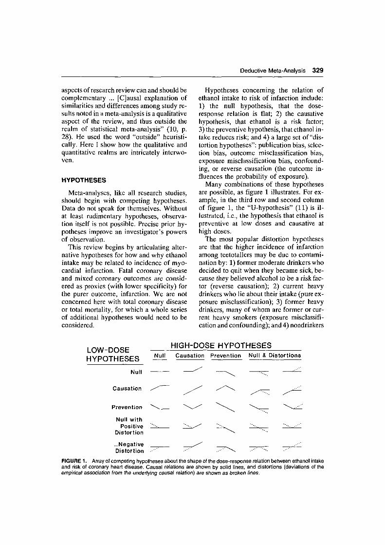
Many combinations of these hypothesesare possible, as figure 1 illustrates. For ex-ample, in the third row and second columnof figure 1, the "U-hypothesis" (11) is il-lustrated, i.e., the hypothesis that ethanol ispreventive at low doses and causative athigh doses.

The most popular distortion hypothesesare that the higher incidence of infarctionamong teetotallers may be due to contami-nation by: 1) former moderate drinkers whodecided to quit when they became sick, be-cause they believed alcohol to be a risk fac-tor (reverse causation); 2) current heavydrinkers who lie about their intake (pure ex-posure misclassification); 3) former heavydrinkers, many of whom are former or cur-rent heavy smokers (exposure misclassifi-cation and confounding); and 4) nondrinkers

HIGH-DOSE HYPOTHESESLOW-DOSEHYPOTHESES

Null

Causation

Prevention

Null withPositive

Distortion

...NegativeDistortion

Null

^ ~

^

—

Causation Prevention Null & Distortions

— ^—

\ ^ \̂ 1

' " - • • • . , . . " • - • • . - - ' '

. . - - • • • • - • . - - • • " '

FIGURE 1 . Array of competing hypotheses about the shape of the dose-response relation between ethanol intakeand risk of coronary heart disease. Causal relations are shown by solid lines, and distortions (deviations of theempirical association from the underlying causal relation) are shown as broken lines.

330 Maclure

who are more sedentary and obese than theaverage drinker, or who get more of theirdietary energy from fats than the averagedrinker (pure confounding).

Among the consequences of beginning ameta-analysis with a set of hypotheses are:1) a broader search of the literature for evi-dence, preferably meta-analyses, concern-ing competing hypotheses (e.g., the rela-tions of ethanol intake to Type A personalityand of Type A personality to heart disease);2) greater alertness to such evidence in re-ports from studies of the causal relation ofinterest (e.g., calculation of an estimate ofselection bias by comparing components ofa hospital control group); and 3) categori-zation of studies by more study character-istics pertinent to tests of competing hypoth-eses in meta-regression (e.g., whether ex-drinkers were excluded from the nondrinkergroup).

METHODS

Like a deductive approach to multivariateanalysis (2), a deductive meta-analysispresents not a single conclusion but a de-scription of the survival or refutation of hy-potheses over a course of tests against dataand against each other. From the first stageof selecting evidence to the final sensitivityanalyses and writing of the report, the goalis to discriminate among competing hypoth-eses.

Selection of studies

An important competing hypothesis isthat publication bias has distorted the overallrelation between ethanol and infarction inthe total body of published data. Trackingdown all unpublished data may be the bestway of avoiding publication bias whenmeta-analyzing randomized controlled tri-als, but with nonexperimental studies, thereis no clear criterion analogous to "all pa-tients randomized." "All patients studied"would include any cohort, case-control,cross-sectional, or even ecologic study thatcollected data on alcoholic drinks and heartdisease. Thus, including all published and

retrievable unpublished reports may makea meta-analysis of nonexperimental datamore, rather than less, susceptible to publi-cation bias. This is a special case of the wellknown trade-off between precision and bias,i.e., between quantity and quality of data.

To refute publication bias, sometimes itmay be better to restrict the meta-analysis tostudy populations that are relatively immuneto the bias. In the case of ethanol and in-farction, recent reports giving data on mul-tiple covariates from large, well known co-horts with ongoing funding are probablyrelatively immune compared with the aver-age case-control study. However, even in-vestigators of well known cohorts are aptto delay publication until an association"achieves statistical significance."

The present meta-analysis aimed for aninitially inclusive selection of studies, but intesting of competing hypotheses, the selec-tion was inevitably whittled down to thoseproviding the best data, i.e., those most re-sistant to uncertainty concerning competinghypotheses. Studies published between1968 and early 1993 were identified by aMEDLINE® search (National Library ofMedicine) and were supplemented with ad-ditional references cited in previous reviews(11, 12). This review focused on data from42 reports (13-54). Twenty-seven reports(55-81) were immediately excluded, mainlybecause of overlapping data, but also be-cause of weaknesses: use of prevalent cases(72, 78), crude exposure groupings (58, 63,64, 76, 81), a combination of mixed out-comes and small numbers (66, 69, 75), orlimited analyses (55, 60, 61). Criteria forchoosing which reports to include whenthere were multiple reports from the samecohort were (in order of priority):

1. Nonfatal myocardial infarction wasthe outcome, because fatal and mixedoutcomes have lower specificity.

2. Ethanol intake was categorized inmore detail, because this enabled bet-ter assessment of the shape of the dose-response curve.

3. Cases were more numerous.


Data from some of the omitted reportswere used in subsidiary analyses. Data re-lated to competing hypotheses were soughtfrom sources other than studies of ethanoland heart disease but less systematically, aweakness discussed below.

Data extraction and unification

For testing of exposure misclassificationbias, some studies (58, 63, 64, 76, 81) wereexcluded because of inadequate exposureassessment. For example, the Walnut CreekContraceptive Drug Study (58) classifiedsubjects only as drinkers or nondrinkers, andthe study of Italian rural men (81) had, as thelowest category of intake, 40 g/day or lessof ethanol.

The quality of exposure information in theincluded studies varied greatly. All studiesused self-reported beverage consumptionfrequencies, but some (16, 19, 20, 22, 38,53) asked only one question about alcoholicbeverages, rather than separate questions forbeer, wine, and liquor. There were large dif-ferences in time periods to which the ques-tions referred: the 24-hour period before theinterview (26), the past 2-3 days (45), thepast week (39, 49), the past month (30, 36,52), the past year (22, 27-29, 51), and"usual" frequency (table 1). The number oflevels of intake into which subjects wereclassified ranged from two to more than 10.

A level of ethanol intake was assigned toeach relative risk using the following algo-rithm:

1. If the mean intake of alcoholic drinkswithin a subgroup was provided orcould be estimated from a table orgraph of the distribution, the only con-version made was to express intake ingrams of ethanol per day, assumingthat one drink contains 13 g of ethanol.

2. If the paper defined subgroups usingcontiguous intervals of ethanol levels(e.g., 0.1-1.0, 1.1-29, and >30ounces/month), the cutpoints wereconverted to grams of ethanol per dayand the mean intake in each intervalwas estimated, assuming that the studyhad the same distribution of alcohol in-

takes as the National Health InterviewSurvey (82).

3. If subgroups were defined by the mostcommon values (e.g., <1, 1-2, or >3drinks/day), then the scale was con-verted to a set of contiguous intervals,picking logical cutpoints between thecommon values (e.g., 0.75 drinks/dayas the cutpoint between <1 and 1-2drinks/day); the cutpoints were con-verted to grams of ethanol per day, andthe mean for each interval was esti-mated as indicated above.

4. When subgroups were defined in moreunusual ways, these were translatedinto contiguous intervals as well aspossible, and the above steps wereimplemented.

For testing the hypothesis that the dose-response curve was distorted by error in thisalgorithm, sensitivity of the results to ex-posure classification was assessed by chang-ing assumptions and repeating the regres-sions.

Quadratic meta-regression

To test competing hypotheses fairly, weneed a method of meta-regression that doesnot force one shape on the data. In theAlbany Study (47), for example, the regres-sion forced a straight line and obscured aU-shape apparent in the crude data. Qua-dratic regression accommodates many moreshapes than does linear regression. Recentlya method (83) was described for quadraticmeta-regression of dose-response data,which takes account of the fact that dose-specific relative risks are never independent.(Their interdependence arises from sharingthe same reference group, and results indouble—or multiple—counting of the un-certainty of the denominator of each ratio.)The one-step "pool-first" method was used:The dose-specific confounder-adjustedlogarithms of the relative risks from all stud-ies were pooled, and a curve was fitted byweighted quadratic regression. The weightswere the inverses of the covariance-adjusted

332 Mad u re

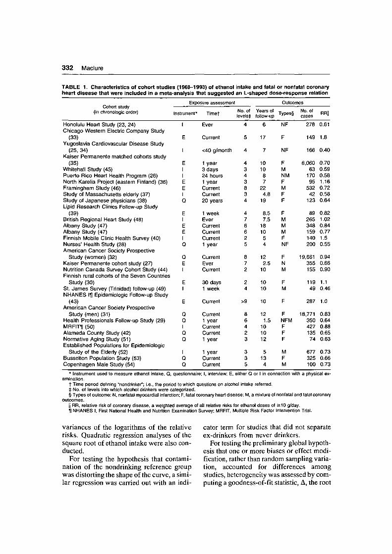
TABLE 1. Characteristics of cohort studies (196S-1993) of ethanoiheart disease that were included in a meta-analysis that suggested

Exposure assessment

(in chronologic order) Instrumeni

Honolulu Heart Study (23, 24)Chicago Western Electric Company Study

(33)Yugoslavia Cardiovascular Disease Study

(25, 34)Kaiser Permanente matched cohorts study

(35)Whitehall Study (45)Puerto Rico Heart Health Program (26)North Karelia Project (eastern Finland) (36)Framingham Study (46)Study of Massachusetts elderly (37)Study of Japanese physicians (38)Lipid Research Clinics Follow-up Study

(39)British Regional Heart Study (48)Albany Study (47)Albany Study (47)Finnish Mobile Clinic Health Survey (40)Nurses' Health Study (28)American Cancer Society Prospective

Study (women) (32)Kaiser Permanente cohort study (27)Nutrition Canada Survey Cohort Study (44)Finnish rural cohorts of the Seven Countries

Study (30)St. James Survey (Trinidad) follow-up (49)NHANES IH Epidemiologic Follow-up Study

(43)American Cancer Society Prospective

Study (men) (31)Health Professionals Follow-up Study (29)MRFITTl (50)Alameda County Study (42)Normative Aging Study (51)Established Populations for Epidemiologic

Study of the Elderly (52)Busselton Population Study (53)Copenhagen Male Study (54)

I

E

I

EIIEEIQ

EIEEIQ

QEI

EI

E

QQIQQ

IQQ

t* Timet

Ever

Current

<40 g/month

1 year3 days24 hours1 yearCurrentCurrent20 years

1 weekEverCurrentCurrentCurrent1 year

CurrentEverCurrent

30 days1 week

Current

Current1 yearCurrentCurrent1 year

1 yearCurrentCurrent

intake and fatal or nonfatal coronaryan L-shaped dose-response relation

No. oflevels^

4

5

4

4343834

476625

872

24

>9

86423

335

Years offollow-up

6

17

7

101087

224.8

19

8.57.5

181054

122.5

10

1010

10

121.5

101012

5134

Outcomes

Types§

NF

F

NF

FMNMFMFF

FMMMFNF

FNM

FM

F

FNFMFFF

MFM

No. ofcases

278

149

166

8,06063

17095

53242

123

89265348159140200

19,661355155

11949

287

18,77135042713574

677325100

RR[|

0.61

1.8

0.40

0.700.590.581.160.720.580.64

0.821.020.840.771.50.55

0.940.660.90

1.10.46

1.0

0.830.640.880.650.63

0.730.660.73

* Instrument used to measure ethanoi intake. Q, questionnaire; I, interview; E, either Q or I in connection with a physical ex-amination.

t Time penod defining "nondrinker"; i.e., the period to which questions on alcohol intake referred.t No. of levels into which alcohol drinkers were categorized.§ Types of outcome: N, nonfatal myocardial infarction; F, fatal coronary heart disease; M, a mixture of nonfatal and fatal coronary

outcomes.ii RR, relative risk of coronary disease, a weighted average of all relative risks for ethanoi doses of ==10 g/day.11 NHANES I, First National Health and Nutrition Examination Survey; MRFIT, Multiple Risk Factor Intervention Trial.

variances of the logarithms of the relativerisks. Quadratic regression analyses of thesquare root of ethanoi intake were also con-ducted.

For testing the hypothesis that contami-nation of the nondrinking reference groupwas distorting the shape of the curve, a simi-lar regression was carried out with an indi-

cator term for studies that did not separateex-drinkers from never drinkers.

For testing the preliminary global hypoth-esis that one or more biases or effect modi-fication, rather than random sampling varia-tion, accounted for differences amongstudies, heterogeneity was assessed by com-puting a goodness-of-fit statistic, A, the root


weighted-mean square of the residual devia-tion (on the logarithmic scale) of each ob-served relative risk (RR,) from the corre-sponding relative risk predicted by theregression (RR,p):

ln RRip)2y(n - t)}™,

where n is the number of relative risks, w, isthe weight given to each RR (the covari-ance-adjusted inverse variance of the loga-rithm of RR,), and t is the number of termsin the regression model (84, 85). The sum-mation in the numerator of A has a chi-squared distribution with n - t degrees offreedom. If each study population were aperfect random sample from a single com-mon source population, the expected valuefor A would be about 1.0. If the observed Ais significantly greater than 1.0, it represents"beyond-random" variation (i.e., heteroge-neity) among relative risks, and serves as acrude estimate of the net systematic varia-tion caused by bias or effect modification.Possible causes of heterogeneity were ex-plored by deleting individual studies thatappeared to be outliers, by deleting certaintypes of study, or by repeating the regressionwith indicator terms for study flaws andcharacteristics.

For testing the hypotheses that weakerstudy designs and nonspecific outcomemeasures were distorting results, separatequadratic meta-regressions were carried outfor: 1) case-control studies of nonfatal in-farction (13-18); 2) case-control studies ofcoronary deaths (19-22); 3) case-controlstudies with population controls, combiningboth nonfatal and fatal cases (18-22); 4) co-hort studies with nonfatal infarction as theoutcome (23-29); 5) cohort studies withcoronary death as the outcome (28-30, 33-41, 43, 50, 51, 53, 54), excluding the hugeAmerican Cancer Society studies (31, 32),which had more cases than all other cohortscombined; 6) cohort studies with other ormixed outcomes: coronary artery bypassgrafts or percutaneous transluminal coro-nary angioplasty (29); a combination of non-fatal and fatal heart disease, including an-

gina (26,46,47,49); coronary insufficiency(26); or cardiovascular death includingstroke (44,45,48,52); and 7) cohort studiesof women with any cardiovascular outcome(27, 28, 32, 35, 37, 39, 41-44, 46, 53, 58).

Incremental relative risks andregression

Even a quadratic model may distort adose-response relation: A kink in the truecurve may be smoothed over. Given enoughdata, therefore, shape is better assessed us-ing nonparametric methods; for example,incremental relative risks (86) or movingline regression (87).

Dose-specific relative risks from all co-hort studies were pooled for an incrementalregression, a variation on moving line re-gression, as follows. The first step was aregular weighted linear regression between0 and 2.0 g/day of ethanol. No intercept termwas used, thus forcing the line through theorigin. A meaningful central point on thisfirst regression line—0.8 g/day (about twostandard drinks per month), at which therelative risk was 0.95—was taken as the ori-gin for the next weighted regression, in theinterval 0.8-5.0 g/day. At a meaningful cen-tral point in this next interval—3.8 g/day(about two drinks per week), the coefficientrepresents the logarithm of the incrementalrelative risk for an increase from two drinksper month to two drinks per week. By re-peating this process, the dose-response re-lation was described for dose incrementsfrom two drinks per week to four drinks perweek to one, two, five, and about 10 drinksper day. Similar incremental regressionswere carried out with varying bandwidths.After an L-shape was found (i.e., a drop inrisk at low doses, followed by a plateau inrisk above one drink per day), overall non-incremental regressions were carried out as-suming an L-shape.

For retesting the hypothesis that higherincidence in nondrinkers was due to con-tamination of the nondrinkers with ex-drinkers, incremental analyses were re-peated in the low-dose range, limited to datafrom studies that separated ex-drinkers from

334 Mad u re

nondrinkers and had a category of occa-sional (less than daily) drinkers (23, 27, 35,38, 42), and by including in the meta-regression an indicator term for studies thatdid not separate ex-drinkers from non-drinkers.

Quantifying bias

Rather than addressing the possibility ofconfounding and misclassification bias sim-ply qualitatively, the magnitude of con-founding was estimated by computing arelative risk ratio where possible. For ex-ample, the crude relative risk before age ad-justment was divided by the age-adjustedrelative risk to obtain the relative risk ratiofor age. This ratio represents the spuriousrelative risk that would have been observedif age were the only confounder and ethanolhad no causative or preventive effect. It is anestimate of the parameter U, which quanti-fies confounding (10). Greenland advocatesadjusting relative risks using these ratios(10,88). Such adjustments should be treatedas sensitivity analyses, and ideally shouldincorporate information on uncertainty ofthe ratio estimates. In this meta-analysis,such adjustments were not made, becausewith so many good large cohort studies, itwas possible to analyze separately in the re-gression those studies with adequate internaladjustments. The relative risk ratio was alsoused to quantify possible bias due to non-differential misclassification.

Inclusion of study characteristics inregressions

For testing the hypothesis that a particularcombination of study flaws might accountfor the association, multivariate meta-regressions were performed. Indicator termswere assigned to individual relative risks orstudies, indicating the presence or absenceof a study flaw (e.g., contamination of non-drinkers with ex-drinkers, a nonspecific out-come measure, no control of confoundingby age). When the study characteristic couldbe quantified, ordinal or continuous vari-ables were assigned (e.g., number of expo-sure categories, number of years of follow-up). The model was fitted by "forward

elimination" (2), i.e., starting with the crudeassociation of interest and adding terms forpotential biases to see which combinationsof study flaws and characteristics might ex-plain the association, based on the change-in-estimate criterion (89).

Some authors use additional qualityweighting according to a systematic assess-ment of study quality by a panel of reviewers(90). This can be viewed as analogous toexpanding the confidence interval of eachrelative risk to reflect the panel's judgmentof the amount of additional uncertainty dueto departures from perfect study quality. Theweaknesses of this approach are that it at-tributes no directionality to the uncertainty(the confidence interval is widened equallyin both directions) and it assigns a magni-tude of uncertainty based more on personaljudgment than on the data at hand. By con-trast, multivariate meta-regression of rela-tive risks on study characteristics allows es-timation of the directionality and magnitudeof bias (i.e., the relative risk ratio) attribut-able to each hypothesized flaw, conditionalon other hypothesized flaws. Thus, multiplehypotheses about distortions can be tested.

RESULTS

Refutation of publication bias

In his meta-analysis of coffee intake andcoronary risk (89), Greenland cited 14 co-hort studies, seven (91-97) of which did notcontribute to the present meta-analysis be-cause I found no published reports fromthem concerning ethanol intake. The sevencohorts yielded a total of 2,378 coronaryoutcomes, which compares with 38,432cases from the American Cancer Societystudies and 19,413 from the other cohortsincluded in this review. Let us assume thatall of these cohort studies had data on etha-nol intake and, to be conservative, that theassociation in these studies between ethanoland coronary disease was positive (i.e., inthe opposite direction from what is reportedhere). Suppose the average relative risk inthese other cohorts were 1.2, because if ithad been greater we would expect to haveseen reports of significant positive associa-


tions. This would amount to a hypotheticalrelative risk ratio of 1.02 for publication biasdue to exclusion of these cohorts. Such aweak bias would have negligible influenceon our conclusions.

The relation of ethanol intake to risk ofheart disease has been a prominent contro-versial topic for long enough that null find-ings should now be as interesting and pub-lishable as non-null results. In the presentreview, therefore, publication bias was con-sidered reduced in analyses that effectivelywere restricted to recently reported cohortstudies. It turned out that controlling forstudy quality in the meta-regressions effec-tively controlled for recency of publication,because the quality of design and analysis ofepidemiologic studies has improved overthe decades. The best studies are the recentlypublished large cohort studies that use mul-tivariate methods.

On the basis of this evidence and the qual-ity of excluded reports, I hypothesize thatexclusion of unpublished and inadequatelyanalyzed data from the meta-regressionprobably did not produce much bias. Un-fortunately, the alternative explanation, thatpublication bias is a major cause of the ob-served association, will remain unrefuteduntil further empirical studies of publicationbias are carried out (98, 99).

Publication bias also operates against evi-dence concerning competing hypotheses.Analyses of selection bias and misclassifi-cation bias at low doses of alcohol consump-tion are hard to find (although there is a greatdeal of literature concerning heavy drink-ers). Although I found some meta-analysesconcerning potential confounders (100-103), a more thorough search of the litera-ture for ancillary data concerning hypoth-esized confounders was not within theresources available. Even within the studiesof ethanol and infarction themselves, therewas plenty of "semi-publication" bias; mostreports gave only glimpses of the impact ofadjusting for covariates.

Refutation of selection bias

It was not possible to refute selection biasor recall bias as an explanation for the as-

sociations seen in case-control studies. Theheterogeneity among relative risks fromcase-control studies was much greater thanwould be expected from random samplingvariation (A = 2.4; p < 0.001). Such het-erogeneity could be due to bias or effectmodification. Repetition of regressions afterdeletion of outliers indicated that the het-erogeneity was not due to a few deviantpoints or a single deviant study.

Selection bias probably occurred in stud-ies with hospital controls (13-16). In two(13, 16) of those studies, patients with cho-lecystectomies or trauma were not excludedfrom the control groups; gallstones and ac-cidents are now known to be related to etha-nol intake (104,105). In two others (14,15),40 percent of the controls had been admittedfor disc disorders. Both studies found thesame elevated ethanol intake among patientswith disc disorders as compared with theother hospital controls, equivalent to a rela-tive risk of 1.3. If this finding is real,it would have exaggerated the ethanol-infarction association, corresponding to arelative risk ratio of 0.88 for occasionaldrinking (table 2). Excluding studies withhospital controls (13-17) only slightly re-duced the heterogeneity (A = 2.2). Inclusionof indicator terms for women and fatal out-comes in the meta-regression (table 2) fur-ther reduced the heterogeneity (A = 2.0; p< 0.001), but it was still too large.

Although effect modification is a possibleexplanation for the large remaining hetero-geneity, we cannot rule out selection bias,especially because the exposure ofinterest—alcohol drinking—is believed tobe related to sociability and antisocial be-havior in complex ways. Therefore, to guardagainst selection bias, I excluded case-control studies from further meta-analyses.Data from population-based case-controlstudies are shown in figure 2.

Refutation of chance

Each of the three quadratic meta-regressions of cohort data yielded similar re-sults: a significant inverse association withsignificant positive curvature (table 3). Qua-dratic models fitted well to relative risks for

336 Maclure

TABLE 2. Estimated relative risk ratios for hypothesized sources of bias and effect modification incase-control studies of ethanol intake and risk of coronary heart disease

Source RRR* 95% Cl* Studies Estimation

Hospital control bias 2.1 0.5-8.5 All case-control RR for 10 g/day of ethanol from meta-regressionstudies (13-22) of data from hospital case-control studies divided

by the same RR for population control studies.

Hospital control bias 0.88 0.77-1.0 Northeastern US 1 + 0.40 x (RR - 1), where RR is the odds ratiostudies (14,15) for drinkers vs. nondrinkers, comparing controls

with disc disorders (40%) with the rest of thehospital controls.

0.4-1.0 Studies with RRR for fatal outcomes relative to the RR forpopulation nonfatal outcomes from meta-regression,controls (18-22) assuming an L-shaped dose-response curve.

0.4-0.8 Studies with RRR for females relative to the RR for males frompopulation meta-regression.controls (18-22)

• RRR, relative risk ratio, the ratio of the unadjusted relative risk (RR) to the adjusted relative risk; Cl, confidence interval.

Proxy interviewee for 0.7deceased cases,controls

Effect measuremodification

0.6

RR1.4 r

1.2

0.8

0.6

0.4

0.2

I I I I I

10 100

Ethanol Intake (g per day)FIGURE 2. Estimates of the relative risk (RR) of coronary heart disease in relation to ethanol intake, from popu-lation-based case-control studies. Circles represent relative risks from studies of nonfatal myocardial infarction andcrosses those from studies of fatal coronary heart disease.

nonfatal infarction (A = 1.10; p = 0.1) andmixed outcomes (A = 1.15; p = 0.1), but notwell for fatal disease (A = 1.7; p < 0.001).The fit for fatal outcomes was little im-proved (A = 1.7) by inclusion of terms for

study flaws and characteristics (inclusion ofex-drinkers with nondrinkers, no control forage, no control for smoking, number ofyears of follow-up, number of exposure cat-egories). Exclusion of the relative risks from


TABLE 3. Quadratic models of weighted logarithms of dose-specific relativestudies of ethanol intake and risk of nonfatal myocardial infarction (Ml), fataldisease (CHD), and mixed CHD outcomes*

Outcome

NonfatalFatal CHDMixed CHD

fHX)

-21.3-6.6

-11.0

Regression coefficientsf

SE§

3.50.72.5

J3(X*)

0.1570.0590.092

Goodnessof fit

SE (P)

0.042 0.10.008 <0.0010.026 0.1

risks from cohortcoronary heart

Risk for £10 g/day(£1 drink/day)*

RR§

0.820.940.90

95% Cl§

0.76-0.890.91-0.970.85-0.96

* Weights were inverses of covanance-adjusted variances of the logarithms.t Change in the logarithm of the relative risk per g and per g2 of ethanol intake.t Reference group was nondrinkers.§ SE, standard error (x10-3); RR, relative risk; Cl, confidence interval.

the American Cancer Society female cohort(32) reduced A to 1.5 (p < 0.001).

Incremental regression clarified the shapeof the curve. Combining all cohort data,there appeared to be a decline in risk at dosesup to one half drink per day, with little fur-ther change in risk associated with drinkingmore than one half drink per day (table 4 andfigure 3). The resulting L-shape resembles asaturation effect, as if all of the hypothesizedprotective effect occurred at low doses.

Combining relative risks for all threetypes of outcomes, the fit of a quadraticmodel (A = 1.6; p < 0.001) was no betterthan that for an L-shaped curve that was lin-ear between 0 and 10 g of ethanol per day,with saturation (flattening) above 10 g/day(A = 1.6). Addition of indicator terms forfatal and mixed outcomes, ex-drinkers in thenondrinker group, no control for age, nocontrol for smoking, control for fewer thanfour variables, and female subjects reduced

TABLE 4. Incremental relative risks (iRRs) for each increment in ethanol intake, and correspondingdose-specific relative risks (RRs), from cohort studies of ethanol intake and coronary heart disease

Frequency ofconsumption(no. of drinks)

0

2/month

2/week

4/week

1/day

2-3/day

4-6/day

£7/day

Ethanolintake(g/day)

0

0.8

3.8

7.5

13

30

60

120

iRR»

0.95

0.92

0.88

1.19

0.91

0.97

1.17

95% Clf

0.73-1.24

0.88-0.97

0.76-1.01

1.07-1.31

0.85-0.98

0.88-1.08

1.02-1.34

RR*

1.0

0.95

0.88

0.77

0.91

0.83

0.81

0.95

chiftpHOl IIILwLI

95% Cl§

Reference

0.73-1.24

0.83-0.92

0.67-0.89

0.82-1.01

0.77-0.89

0.73-0.90

0.83-1.09

• The iRR is the relative risk comparing consecutive levels of ethanol intake. The reference group is the subgroup of drinkerswith less intake; the index group is the subgroup with greater intake. The iRRs were estimated by incremental weighted regression(a variation on moving line regression; see text) of logarithms of the RRs in the index interval, with weights equal to inverses ofcovanance-adjusted variances of each of the RRs in the interval. Instead of RR = 1 at 0 g/day, the origin for the regression wastaken as the RR at a midpoint in the reference interval, i.e., at the level of intake specified in the first column of the preceding rowof the table. The 95 percent confidence intervals were widened by multiplying the standard error by the residual deviance to accountfor heterogeneity among RRs in the index interval.

t Cl, confidence interval.t The RR for a given intake of ethanol was derived from the iRRs for the component increments (i.e., the product of the iRRs

in the preceding rows).§ The shifted 95 percent confidence interval is the 95 percent confidence interval of the iRR in the preceding row, shifted so that

it is centered on the RR; it is a minimum estimate of the uncertainty of the RR.

338 Mad u re

RR

0.5

0.10 10 20 30 40 50 60 70 80 90 100 1 10 120 130 140

Ethanol Intake (g per day)FIGURE 3. L-shaped relation between the relative risk (RR) of coronary heart disease and ethanol intake, basedon meta-analysis of relative risks from all cohort studies (shown as points). Squares and error bars show RRs and95% confidence intervals (adjusted for heterogeneity) of dose-specific weighted averages of RRs. The line was fittedby incremental weighted regression (a kind of moving line regression; see text), with weights equal to the inverseof the covariance-adjusted variance of the logarithm of the RR.

A to 1.4 (p < 0.001). After adjustment of thevariances for this residual heterogeneity, therelative risk for intake of 6.5 g/day (a drinkevery other day) was 0.76 (95 percent con-fidence interval (CI) 0.65-0.90). This vir-tually refutes the null hypothesis that the as-sociation was "due to chance." However,this means only that an unlikely scenariowas refuted: that Nature had randomly as-signed ethanol intake to the study subjects,yet there still occurred a chance imbalanceof confounders (106).

To refute the possibility that the complex-ity of the meta-regression was obscuring theanalysis, I also carried out simpler analyses.Weighted regression of low-dose data fromfive studies (23, 27, 35, 38, 42) that sepa-rated ex-dririkers from long-standing non-drinkers gave an estimated relative risk of0.83 (95 percent CI 0.67-1.01) for one halfdrink per day in comparison with never

drinkers. Excluding nondrinkers altogetherand using occasional drinkers as the refer-ence group in five other studies (28, 29, 46-48), it was possible to estimate an incremen-tal relative risk of 0.88 (95 percent CI 0.81-0.96) for approximately one drink per dayrelative to less-than-daily drinking: Thisagrees with the corresponding incrementalrelative risk of 0.91 (95 percent CI 0.88-0.95) from the American Cancer Societystudies (31, 32).

These meta-regressions of cohort dataconfirm that a generalizable association ex-ists (is not due to chance), but they do notexplain why it exists.

Refutation of outcome misclassificationbias

A recent review (107) of error in diagno-sis of coronary heart disease concludederroneously that cardiologic epidemiologic


studies are unreliable because their data areinaccurate. The author overlooked the dis-tinction between insensitivity and nonspeci-ficity of the diagnosis. By making thisdistinction, we shall see that outcome mis-classification cannot account readily for theethanol-infarction association.

Diagnosis of nonfatal myocardial infarc-tion. It is estimated that half of all myocar-dial infarctions may be silent (108). In ad-dition, many infarctions are fatal. Therefore,the diagnosis of nonfatal myocardial infarc-tion is clearly very insensitive to the trueincidence. However, a relative risk would beunaffected by insensitivity if 1) nonspeci-ficity is negligible (109) and 2) the insen-sitivity is no greater among drinkers thanamong nondrinkers. The specificity of thediagnosis of myocardial infarction, whenconfirmed by chest pain, electrocar-diography, and elevated cardiac enzymes,appears to be so high that leading researchdoes not even discuss it (110). False positivediagnoses due to myocarditis are rare (111).On the other hand, insensitivity conceivablycould be differential: The anesthetic effectof ethanol might mask infarction symptomsor influence survival. However, a reviewer(112) judged the evidence to be contradic-tory and inconclusive on the relation of etha-nol intake to pain among angina patients.Moreover, differences in pain sensitivitywould not readily explain the inverse asso-ciation between ethanol intake and coronarydeath. Likewise, the inverse associationwith coronary death is opposite what onewould expect if the association with nonfatalinfarction was due to ethanol's causingpoorer survival after infarction.

Diagnosis of fatal coronary disease. Adiagnosis of coronary heart disease on adeath certificate has less specificity than fa-tal acute myocardial infarction. For ex-ample, a major type of heart disease, suddencardiac death, appears to have a positive pre-dictive value of less than 80 percent as aproxy for fatal infarction, based on a studyof resuscitated patients (113). Assumingthat false positive diagnoses occur equallyamong nondrinkers and drinkers, calcula-

tions show that a relative risk of 0.8 for sud-den fatal infarction among drinkers wouldbe manifest as a relative risk of about 0.93for sudden cardiac death as a whole. Thiswould partly explain the weaker relation ofethanol to fatal outcomes than to nonfataloutcomes.

Loss to follow-up. Insensitivity of theoutcome measure increases with loss tofollow-up. However, in the major cohortstudies (27-32), losses to follow-up wereless than 3 percent. Only if loss were verystrongly related to nonfatal disease wouldany bias be more than negligible in thesestudies.

In conclusion, we can rule out inaccuracyof diagnosis as an explanation for the ap-parent reduction in incidence of coronarydisease at low ethanol intakes, but it couldpartly explain the flatness of the curve frommoderate doses to high doses.

Refutation of exposuremisclassification bias

Self-reported alcohol consumption iswidely believed to be inaccurate. Differen-tial recall, however, is mainly a problem forcase-control studies, which we have alreadyexcluded. Exposure misclassification inprospective cohort studies would tend to benondifferential (especially after stratifica-tion by risk group), because responses to thealcohol questions in the interview or on thequestionnaire cannot be influenced by ill-ness that has not yet occurred.

Underreporting. Most error in self-reported current alcohol intake is believedto be insensitivity, i.e., underreporting(114). This is sometimes compounded byinsensitive questions. In the AmericanCancer Society study (31, 32) and the Mul-tiple Risk Factor Intervention Trial (50), the"nondrinker" category must have includedfalse negatives: drinkers who got their etha-nol from beverages other than beer, wine, orwhiskey. In the Puerto Rico Heart HealthProgram (26), the "unexposed" category in-cluded drinkers who happened to have ab-stained within 24 hours of the interview.Despite the resulting tendency for relative

340 Maclure

risks to be biased toward the null, these stud-ies showed significant associations.

Misclassification within drinkers. It iseasier to remember whether or not you everdrank ethanol than to remember how oftenand how much. Therefore, incremental rela-tive risks across different levels of drinking(excluding nondrinkers) might be more di-luted toward the null, because of nondiffer-ential misclassification, than relative risksfor all drinkers versus nondrinkers. In theextreme, such unequal misclassificationcould cause various dose-response relations(continuously decreasing, U-shape) to bemanifest as an L-shape.

How much flattening can be attributed toerror in reporting of alcohol intake? Vali-dation studies conducted within the Nurses'Health Study (115) and Health ProfessionalsFollow-up Study (116) cohorts found thatSpearman correlation coefficients of valid-ity (comparing intakes measured by foodfrequency questionnaires and by the averageof four 1-week diet records) were 0.90 inwomen and 0.86 in men. The amount of biastoward the null caused by nondifferentialexposure misclassification is a function ofthe coefficient from a regression of "true"ethanol intake on the mismeasured variable(117). In the Nurses' Health Study, the co-efficient was 0.67, which suggests that re-gression slopes may have underestimatedthe true slope by about 45 percent (117).

Irregular drinking. Most studies did notseparate irregular drinkers from regulardrinkers. From the British Regional HeartStudy (48), we can calculate a relative riskof 1.2 (95 percent CI 0.83-1.9) among menwho had 3-6 drinks per day on weekendsonly versus daily drinkers of 1-2 drinks perday. In the American Cancer Society study(31), irregular drinkers had an age- andsmoking-adjusted relative risk of 1.2 (95percent CI 1.1-1.3) relative to men who had1-5 drinks per day. These data suggest thathigher incidence among moderate irregulardrinkers may obscure the apparent protec-tive effect of regular drinking.

Drift. Although underestimation (insensi-tivity) is probably the main type of error in

measuring current drinking, overestimation(nonspecificity) may be a problem whencurrent drinking is used as a proxy for futuredrinking. Mean intake of alcohol declineswith age in cross-sectional data, but in theUnited States, consumption per capita in-creased in the 1960s and 1970s and declinedin the 1980s (118). Intake increased in theFramingham Study cohort even among pa-tients with prior diagnoses of heart disease(46). In the Alameda County Study (42),drift of people away from their baseline sta-tus as a drinker or nondrinker was equal toa decline in positive predictive value ofabout 1 percent per year of follow-up, anda decline in negative predictive value ofabout 3 percent per year. Over 10 years offollow-up, this would produce a 20 percentdilution corresponding to a relative risk ratioof about 1.08. However, in the more recentlarge cohort studies, durations between ex-posure assessment and outcome were tooshort for drift to be important (Health Pro-fessionals Follow-up Study, 1.5 years;Nurses' Health Study, 4 years; Kaiser Per-manente cohort study, 2.5 years).

Ex-drinkers. Shaper (119) hypothesizedthat the U-shaped mortality curve was due tocontamination of the nondrinkers with ex-drinkers. Our meta-analysis allays concern.The weighted average of the relative risksfor ex-drinkers relative to nondrinkers infive cohort studies (23, 28, 38, 42, 77) plusresults from the Health Professionals Study(Eric Rimm, Harvard University, personalcommunication, 1992) was 1.07 (95 percentCI 0.89-1.28). Therefore, although it is de-sirable to separate ex-drinkers from long-term abstainers, failure to do so would usu-ally cause minimal bias. In the meta-regression, the coefficient for failure toseparate ex-drinkers corresponded to a rela-tive risk ratio of 1.05 (table 5). Moreover,both the Nurses' Health Study (28) and theHealth Professionals Study (29) reportedthat the relative risks did not change sub-stantially after exclusion of subjects who re-ported recent changes in their alcohol in-take.

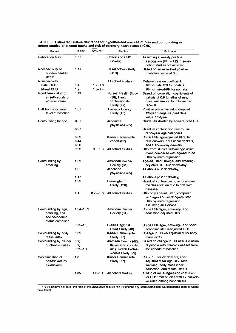
TABLE 5. Estimated relative risk ratios for hypothesized sources of bias and confounding incohort studies of ethanoi intake and risk of coronary heart disease (CHD)

Source RRR' 95% Cl* Studies Estimation

Publication bias

Nonspecificity ofsudden cardiacdeath

NonspecificityFatal CHDMixed CHD

Nonditferential errorin self-reports ofethanoi intake

Drift from exposurelevel at baseline

Confounding by age

Confounding bysmoking

1.02

1.17

1.41.21.17

1.07

0.67

0.97

0.620.440.560.92

1.09

1.0

1.171.02

Coffee and CHD(91-97)

Resuscitation study(113)

All cohort studies1.2-1.61.0-1.4

Nurses' Health Study(28), HealthProfessionalsStudy (29)

Alameda CountyStudy (42)

Japanesephysicians (65)

Kaiser Permanentecohort (27)

0.5-1.8 All cohort studies

American CancerSociety (31)

Japanesephysicians (65)

FraminghamStudy (120)

Confounding by age,smoking, andsocioeconomicstatus combined

1.1 0.79-1.6 All cohort studies

1.04-1.09 American CancerSociety (31)

Confounding by bodymass index

Confounding by history 0.9;of chronic illness 0.9;

0.95-1.1

Contamination ofnondrinkers byex-drinkers

0.95-1.0 British RegionalHeart Study (48)

0.85 Kaiser PermanenteStudy (77)

Alameda County (42);Italian rural cohorts(81); Health Profes-sionals Study (29)

1.0 Kaiser PermanenteStudy (77)

1.05 1.0-1.1 All cohort studies

Assuming a weakly positiveassociation (RR = 1.2) in sevencohort studies not included.

Based on an estimated positivepredictive value of 0.8.

Meta-regression coefficient:RR for fatal/RR for nonfatalRR for mixed/RR for nonfatal

Based on correlation coefficients ofvalidity of 0.9 for ethanoi use;questionnaire vs. four 7-day dietrecords.

Positive predictive value dropped1 %/year; negative predictivevalue, 3%/year.

Crude RR divided by age-adjusted RR.

Residual confounding due to useof 15-year age categories.

Crude RRs/age-adjusted RRs; forrare drinkers, occasional drinkers,and >1 drink/day drinkers.

RRs from studies without age adjust-ment, compared with age-adjustedRRs by meta-regression.

Age-adjusted RR/age- and smoking-adjusted RR (1-2 drinks/day).

As above (< 2 drinks/day)

As above (>2 drinks/day)Residual confounding due to smoker

misclassification due to drift frombaseline.

RRs only age-adjusted, comparedwith age- and smoking-adjustedRRs by meta-regressionassuming an L-shape.

Crude RRs/age-, smoking-, andeducation-adjusted RRs.

Crude RRs/age-, smoking-, and socio-economic status-adjusted RRs.

Change in RR on adjustment for bodymass index.

Based on change in RR after exclusionof people with chronic illnesses fromthe cohorts at baseline.

RR = 1.0 for ex-drinkers, afteradjustment for age, sex, race,smoking, body mass index,education, and marital status.

Antilog of meta-regression coefficientfor RRs from studies with ex-drinkersincluded among nondrinkers.

* RRR, relative risk ratio, the ratio of the unadjusted relative risk (RR) to the adjusted relative risk; Cl, confidence interval (wherecalculable).

342 Maclure

Refutation of hypothesizedconfounders

In this section, we attempt to quantify un-controlled confounding by known risk fac-tors. Unfortunately, only a few studies pro-vide data that enable estimation of relativerisk ratios due to confounding. Moreover,the generalizability of such ratios is prob-ably lower than that of relative risks, be-cause they depend on the magnitudes of cul-turally determined associations betweenalcohol intake and coronary risk factors.

Age. How much of the L-shape from ourmeta-regression could be due to residualconfounding by age? In the study of Japa-nese physicians (65), 15-year age categorieswere used. If 5-year age categories had beenused, the fully adjusted relative risk wouldhave been about 0.91 instead of 0.88, whichgives a relative risk ratio of 0.97 for residualconfounding by age. Comparing this to therelative risk ratio of 0.67 (the crude relativerisk divided by the age-adjusted relativerisk) shows that only about 7 percent of theoriginal confounding by age remained un-controlled. Therefore, since most studiesused narrower age categories than the Japa-nese study, residual confounding by ageseems very unlikely to be an explanation forthe L-shape.

Smoking. Adjusting for smoking causesthe ethanol-infarction association to bestronger, not weaker. The Japanese physi-cian study (65) gave both age-adjusted andage- and smoking-adjusted relative risks forfatal coronary disease. This permits calcu-lation of a relative risk ratio of 1.2 due tosmoking by heavier drinkers. Among lighterdrinkers, the ratio was 1.0, meaning no con-founding. In the American Cancer Societystudy (31), the ratio among men who re-ported having one or two drinks per day was1.1.

How much of the flattening of the curveat higher doses of ethanol might be due toresidual confounding by smoking? Some re-sidual confounding would result from mis-classification of ex-smokers as smokers. Inthe Framingham Study (120), it was shownthat 40 percent of nondrinkers who had been

smokers at baseline were ex-smokers after10 years of follow-up, whereas amongdrinkers the figure was 30 percent. Calcu-lations suggest that this would result in arelative risk ratio of only 1.02 due to residualconfounding by smoking. Additional re-sidual confounding from other kinds of errorin quantifying smoking would tend to biasthe relative risk further upward.

Education and socioeconomic status.Two reports (31, 48) enabled calculation ofrelative risk ratios of 0.95-1.09 for net con-founding by age, smoking, and education orsocioeconomic status, but ratios for educa-tion or socioeconomic status alone were notcalculable (table 5). It appears unlikely thatresidual confounding by education or socio-economic status is an explanation for the as-sociation, but it is possible that these vari-ables are poor proxies for an unmeasuredconfounder with a high relative risk ratio.

Obesity. If obese people were morelikely to be nondrinkers, the ethanol-infarction association could be due partly toresidual confounding by obesity. A review(101) of 51 studies of the relation betweenalcohol intake and adiposity showed noclear overall pattern. The Kaiser Perma-nente study (77), the Honolulu Heart Study(121), and the Nurses' Health Study (122)found that nondrinkers were more likely tobe obese, but this was not found in theHealth Professionals Study (122). In theKaiser Permanente study (77), adjustmentfor body mass index caused the relative riskfor fatal heart disease to attenuate from 0.56to 0.66, which gives a relative risk ratio of0.85. Weight loss was the reason given by 15percent of people who reported having re-duced their intake of alcohol. This subgrouphad a relative risk of 1.4 (95 percent CI0.97-2.0), adjusted for age, sex, race, smok-ing, body mass index, marital status, andeducation.

Physical activity. A more likely source ofresidual confounding is physical activity,because it is much more difficult to measurethan obesity. In fact, only four cohort studies(26, 28, 42, 68) adjusted for measures ofphysical activity. In the Alameda County


Study (42), the adjustment had a negligibleeffect on the relative risk, but this could bemerely because the index of physical activ-ity was poor. A meta-analysis (100) con-cluded that people in sedentary occupationshave a relative risk of 1.9 (95 percent CI1.6-2.2) for coronary disease when com-pared with people in active occupations.This is comparable to the relative risk forsmoking. If the association between a sed-entary lifestyle and nondrinking were asstrong as that between nonsmoking and non-drinking, the relative risk ratio for a seden-tary lifestyle would be between 1.0 and 1.1.

Diet. The vast literature on diet and heartdisease suggests that multiple nutrients in-fluence risk (123). The Honolulu (23),Nurses' (28), and Health Professionals (29)studies adjusted for multiple dietary risk fac-tors, including saturated and polyunsatu-rated fats and cholesterol. Adjustment fornutrients had almost no effect. This is con-sistent with the lack of strong associationsbetween ethanol and nutrient intake in theHonolulu (121), Nurses' (122), and HealthProfessionals (122) cohorts.

The latest hypothesis to be corroboratedin more than one study is that antioxidants,such as vitamin E and beta-carotene, may beprotective. In the Health Professionals co-hort (124), ethanol intake was only slightlyhigher in the lowest quintile of vitamin Eintake. In the Nurses' Health Study (125),there was no association between intakes ofethanol and vitamin E.

The meta-analysis (88) of coffee intakeand risks of fatal and nonfatal heart diseasefound that the relative risks tended to be el-evated among drinkers of five or more cupsper day. In some studies, alcohol drinkersconsume more coffee than nondrinkers(126). Like smoking, this would tend to flat-ten the curve at higher doses but would notexplain the reduction in risk at low doses ofethanol. Two studies (23, 27) adjusted forcoffee intake and found that it did not affectthe association with ethanol.

Medications. Confounding by medica-tions is substantially avoided by restrictingcohorts to subjects without clinical disease.

However, in a healthy population, aspirinuse (127) could magnify the ethanol-infarc-tion association if nondrinkers abstainedfrom aspirin while occasional drinkers tookit frequently. Current use of postmenopausalestrogens in the Nurses' Health Study (128)was associated with an average ethanol in-take of 7.9 g/day, compared with 7.5 g/dayamong former users and 7.3 g/day amongnever users. This would slightly exaggeratethe ethanol-infarction association amongwomen because of the cardioprotective ef-fect of estrogen (128).

Intermediate biochemical markers. Aphysiologic coronary risk factor such ashigh density lipoprotein cholesterol, bloodpressure, or diabetes can be both a con-founder and an intermediate in the causalpathway between ethanol intake and infarc-tion. Not adjusting for it would leave re-sidual confounding; adjusting for it wouldtend to underestimate the association (129).Special methods to control for confoundingby intermediates have only recently been de-veloped (129) and were not used in any ofthe studies reviewed here. Criqui et al. (39)reported that adjustment for high density li-poprotein cholesterol reduced but did noteliminate the ethanol-infarction association.In the Kaiser Permanente cohort study (27),relative risk ratios for blood pressure, serumcholesterol, and glucose ranged from 0.98 to0.90 when these variables were added tomodels that had already adjusted for age,smoking, sex, race, coffee intake, and edu-cation. The Nurses' Health Study (130)found that ethanol may be protective againstthe original development of diabetes, whichwould mean that adjusting for diabetes, as inseveral cohort studies (28,29,43,44,50,52,53), would result in some underestimationof the effect of ethanol.

Refutation of reverse causation

Shaper (119) hypothesized that existingdiseases cause drinkers to quit, such that thenondrinking category becomes contami-nated by ill people. If the illness is heartdisease itself, this would be reverse causa-tion bias. Indeed, in the Kaiser Permanente

344 Maclure

study (77), about 40 percent of ex-drinkerssaid they had quit for medical reasons.Moreover, data from the Alameda CountyStudy (42) and the Italian part of the SevenCountries Study (81) indicate relative riskratios of 0.9 if history of chronic illness istreated as a confounder. However, Shaper'shypothesis was refuted by the large cohortstudies (28, 29, 31, 77), which found thatthe ethanol-infarction association persistedwhen analyses excluded ex-drinkers and/orpeople with chronic illnesses. In the Ameri-can Cancer Society study (31), among the 33percent of men who were "sick at enroll-ment," the prevalence of drinking was ac-tually the same as in the rest of the cohort,and the relative risks for coronary deathwere virtually identical. In the Health Pro-fessionals Study (29), which excluded menentirely if they had a history of cancer, myo-cardial infarction, angina, stroke, or cardiacprocedures, an additional analysis was car-ried out after further exclusions: history ofgout, diabetes, hypercholesterolemia, hy-pertriglyceridemia, hypertension, or otherheart problems. The resulting relative riskratios were 1.1 among occasional drinkersand 0.95 among light drinkers.

In the Kaiser Permanente cohort (77), the50 percent excess in age-adjusted incidenceof fatal cardiovascular outcomes among ex-drinkers as compared with never drinkersdisappeared after adjustment for sex, race,smoking, body mass index, marital status,and education. Similar adjustments did noteliminate the excess incidence of noncardio-vascular death (relative risk = 1.3, 95 per-cent CI 1.0-1.7). This suggests that Shaper'sconcerns may be valid for studies of totalmortality but not for coronary mortality.

Reverse causation could have biased theassociation in several case-control studies(13, 19—21) that included patients who hadhad previous diagnoses of myocardial in-farction.

Refutation of unmeasurableconfounders and biases

In addition to the confounders and biasesmentioned above, there are other potentialexplanatory factors that were not measured

or controlled: stress, personality, lying,physical activity at work, and nonethanol in-gredients of alcoholic drinks. Hill's (131)criteria for causal inference are useful asweak tests of these alternatives. Althoughthey are commonly used as a checklist ofsupporting evidence, we shall see how thecriteria are better treated as criteria for re-futing unmeasurable or unknown confound-ing and bias.

Strength of association. A strong asso-ciation is harder to explain away as beingdue to an unnoticed alternative risk factor.By Hill's definition of strong (131), the re-lation in the ethanol-infarction association isweak. Therefore, it is reasonable to hypoth-esize that life events, Type A behavior, andanger, which are hypothesized to be risk fac-tors for heart disease (132), might be con-founders. These phenomena are difficult tomeasure and, indeed, none of the cohortstudies mentioned controlling for them. Evi-dence for only weak confounding comesfrom a meta-analysis of Type A behaviorand risk of coronary disease which con-cluded that the relation was found only in asubset of studies and was weakened if themeta-analysis weighted studies by size(102). There is some evidence that Type Amen drink more alcohol than Type B men(103). Type A behavior would have to bevery strongly associated with ethanol intaketo produce substantial confounding.

Consistency. Several hypotheses con-cerning unmeasured confounders are re-futed by the fact that the ethanol-infarctionrelation is seen consistently across diversepopulations. If diversity is defined as "largebetween-population variability in the mag-nitude and direction of associations be-tween ethanol intake and confounders,"then diversity can be viewed as quasi-randomization by Nature. This author be-lieves that diversity tends to increase thevariability of the magnitude of confoundingacross studies. There is no reason why theconfounding would tend to cancel out withlarge numbers of studies (as it would in arandomized trial), but if the magnitude ofthe ethanol-infarction association is consis-tent across diverse populations, it is harder


to explain it away as being due to unmea-sured confounders.

The hypothesis that other ingredients ofcertain alcoholic beverages are the actualpreventives, not the ethanol itself, is refutedby the consistency of the association acrossdifferent types of alcoholic drinks.Weighted averaging of the relative risks re-ported for beer, wine, and liquor separatelyin five cohort studies (23, 28, 36, 46, 77),plus data from the Health ProfessionalsStudy (Eric Rimm, Harvard University, per-sonal communication, 1992), gave almostidentical relative risks: 0.78 (95 percent CI0.70-0.87) for beer, 0.74 (95 percent CI0.65-0.85) for wine, and 0.79 (95 percent CI0.72-0.86) for liquor.

Cross-cultural consistency helps rule outdistortion due to drinkers' lying about theirintake and confounding due to an undiscov-ered dietary factor or health-related behav-ior. Reasons for not drinking would prob-ably be quite different among elderlyAmericans who lived through the Prohibi-tion era than among middle-aged Japanesephysicians. The more diverse the culturesare, the more difficult it is to explain theassociation as being due to a cultural allo-cation bias.

The association was consistent betweenthe sexes. A weighted average of relativerisks from studies that included women (27,28,35,37,39,41-44,46,53,58), excludingthe American Cancer Society study, yieldeda relative risk of 0.81 (95 percent CI 0.66-0.98) for occasional drinkers versus non-drinkers. In the female portion of theAmerican Cancer Society study (32), thecorresponding relative risk was 0.87 (95percent CI 0.80-0.93). Regression estimatesof the relative risk ratio for females versusmales ranged from 0.96 to 1.16. This sug-gests that substantial confounding by sex-specific exposures such as estrogen use didnot occur.

Consistency across the age spectrum wasalso seen. A weighted average of the relativerisks for people over 65 from six studies (35,37,57,52,77,133) yielded a relative risk of0.78 (95 percent CI 0.72-0.86) for drinkers

versus nondrinkers. This, plus the consis-tency of the association in the 1960s, 1970s,and 1980s and in both sick and healthypopulations, helps further rule out con-founding by physical activity, medications,or illnesses.

Dose response. The existence of amonotonic trend in risk, i.e., a continuouslyincreasing or decreasing dose-response re-lation (or "biologic gradient"), is a specialcase of the criterion of consistency acrossdiverse subgroups. Here groups differ intheir doses of ethanol. The monotonic trendat low doses (table 4) from incremental re-gression refutes the hypothesis that theethanol-infarction association was entirelydue to contamination of the nondrinkinggroup by ex-drinkers.

If the monotonic trend had continuedbeyond the low-dose range, many of thehypothesized biases and uncontrolled con-founders would have been further dis-credited. As it is, the L-shape leaves criticsa toehold. It is still possible to argue thatthere is confounding by some characteristicof people who seldom or never drink alco-hol.

Plausible mechanism. The lack of asmooth dose-response relation may meanthat some confounders are more difficult torefute, but it is does not rule out causation.The relation between aspirin intake andcoronary risk is believed to be L-shaped, anda plausible mechanism has been demon-strated: Aspirin taken at low doses everyother day produces a sustained reduction inplatelet aggregability—i.e., a saturationcurve (127). It is plausible that ethanol atlow doses has a similar effect (134).

A refutationist is suspicious of mechanis-tic arguments used to bolster the hypothesisof interest. Literature on the biomedical ef-fects of ethanol illustrates the need for sus-picion (135). Ethanol appears to have manyeffects on the circulatory system, some ben-eficial, some adverse. A mechanism can befound to support any prejudice.

The main use of the plausibility criterionshould be to cast doubt on mechanisms that

346 Maclure

are implausible because of their complexity.An example of a less plausible mechanismis the hypothesis that psychological charac-teristics of nondrinkers and heavy drinkerspredispose them to stress, and consequentlyheart disease, whereas occasional and mod-erate drinkers are more emotionally ad-justed. This hypothesis is convoluted withmultiple steps, each of which provides manyopportunities for the association to be di-luted by other causes. By comparison, thedirect biochemical effects of ethanol aremore plausible explanations, because theyinvolve fewer intermediate steps whereother causal factors might intervene.

Coherence. Plausibility is reduced by"incoherent" evidence. For example, theethanol-infarction hypothesis was oncecriticized because evidence seemed to sug-gest that subfraction 2 of high density lipo-protein cholesterol (HDL2) was more pro-tective than subfraction 3 (HDL3). This wasincoherent with the observation that ethanolelevated HDL3 more than HDL2. The inco-herence has since been resolved. Currentevidence suggests that HDL3 is at least asprotective as HDL^ (136).

Analogy. Arguments for mechanisticplausibility often draw on analogies. For ex-ample, ethanol appears to have an analo-gous, apparently protective effect on risk ofsymptomatic gallstones (104), a diseasewhich shares other etiologic factors withcoronary heart disease, such as obesity, lowvegetable intake, and possibly smoking.Like the criterion of plausibility, analogy iseasy to misuse. The use of analogy in a refu-tationist analysis is mainly for generatingcompeting hypotheses. For example, ourconcern about selection bias in case-controlstudies was based largely on analogy withother case-control studies in which selectionbias has been documented (137).

Specificity. Ethanol lacks "specificity ofeffect," because it has multiple biologic andbehavioral effects. Consequently, it is easyto hypothesize biases in case-control studies(e.g., selection bias and recall bias) andin cohort studies (e.g., differential loss tofollow-up and residual confounding). In ad-

dition, coronary heart disease lacks "speci-ficity of cause," because it has a multifac-torial etiology. This means we can easilyadd plausible hypotheses to the list of po-tential confounders. Specificity is a some-what tautologic criterion: It amounts to a re-statement of the principle that causalinference is contingent on lack of alternativeexplanations.

Temporality. The principle that causemust precede effect is used to refute reversecausation. Earlier in this review, we saw thatreverse causation was refuted by restrictingcohorts to subjects who reported no historyof chronic disease.

DISCUSSION

Deductive meta-analysis of evidence forand against more than 20 hypotheses con-cerning the relation between ethanol intakeand incidence of myocardial infarction cor-roborated the preventive hypothesis byweakening competing hypotheses. The de-cline in risk at low doses does not appear tothis author to be due to random samplingvariation, selection bias, reverse causation,or error in measuring ethanol intake or heartdisease. Confounding by an unidentifiedrisk factor that is common in nondrinkersbut not in occasional drinkers is hard toimagine. Residual confounding by a com-bination of factors—obesity, sedentary life-style, aspirin, and diet—is difficult to ruleout, but when I construct such a mixed hy-pothesis, it seems too contrived.

As for the flattening of risk with ethanolintake greater than one drink every otherday, several competing explanations re-main. One is that multiple effects of ethanolon blood cancel each other out and the over-all result is a "saturation effect," a true flat-tening of the preventive relation. Another isthat error in measuring ethanol intake andconfounders among heavier drinkers causesa spurious flattening of the curve. Therefore,the U-hypothesis is not yet conclusively re-futed.


Clinical advice

This analysis suggests that people whohave 2-4 alcoholic drinks per day can safelycut their intake to one drink per day. On theother hand, most health professionals stillrefrain from suggesting that nondrinkersstart drinking small quantities of ethanol(138). Equally effective prevention of heartdisease may be achieved by other means(139), including control of weight and bloodpressure, use of aspirin and possibly anti-oxidant supplements, moderate exercise,and intake of oleic acid instead of saturatedand trans fatty acids.

Meta-analysis controversy

This review has demonstrated that a ref-utationist approach to epidemiologic in-ference is a solution to the problem ofoverinterpretation of meta-analysis in epi-demiology. Meta-analyses should be de-signed as tests of competing explanations,not mere summaries of summaries. Meta-analyses of randomized double-blind trialshave the luxury of focusing on the refutationof chance (random imbalance of net con-founding), because selection bias, informa-tion bias, and nonchance confounding areminimized by randomization and blinding.Meta-analyses of nonexperimental studiesare more difficult, because they must refutemany more competing hypotheses beforecausation can be inferred.

The controversy (1,140-143) about meta-analysis of nonexperimental studies is inlarge part a reaction to the overinterpre-tation of confidence intervals that excludethe null value and overreliance on the con-sistency criterion. The narrowness of meta-confidence intervals merely forces us tograpple with the fact that confidence inter-vals in nonexperimental studies representonly one type of uncertainty, the meaning ofwhich is obscure (106). The consistency cri-terion corroborates the causal hypothesis ofinterest only indirectly by refuting con-founders and biases that differ across stud-ies. It does not refute confounders and biasesthat recur consistently in many studies.

Remaining problems

This meta-analysis could have been morerigorously deductive. Many competing hy-potheses, particularly that of publicationbias, were treated only semiquantitatively.A more thorough search of the literature forancillary data would have been desirablegiven additional resources. With better es-timates of relative risk ratios (including theirvariances and heterogeneity across studies),it would have been fruitful to perform sen-sitivity analyses of the effect of dividing ob-served relative risks by relative risk ratios toadjust for hypothesized study flaws.

Incompleteness is an inevitable charac-teristic of a deductive meta-analysis, forthe same reasons that the combination ofselected variables, transformations, andmodeling assumptions is virtually limitlessin multivariate analysis (89). The open-endedness reflects the manner by whichgeneralizable knowledge grows, but poses achallenge for authors' time, editors' space,and readers' interest. A quick and simplemeta-synthesis is more intelligible at the riskof being misleading. A long and complexdeductive approach is more rigorous at therisk of being unintelligible. The optimumcombination of parsimony and rigor will de-pend on the number of competing hypoth-eses, the quantity of evidence available, andsocial costs of the policy alternatives.

ACKNOWLEDGMENTS

This work was supported by a grant fromAnheuser-Busch, Inc. (St. Louis, MO), admin-istered through the Washington Technical Infor-mation Group, Inc., Washington, DC.

The author thanks Drs. Sander Greenland andMatthew Longnecker for their helpful sugges-tions.

REFERENCES

1. Dickersin K, Berlin JA. Meta-analysis: state-of-the science. Epidemiol Rev 1992;14:154-76.

2. Maclure M. Multivariate refutation of aetiologi-cal hypotheses in non-experimental epidemiol-

348 Maclure

ogy. Int J Epidemiol 1990;19:782-7.3. Kneale W, Kneale M. The development of

logic. Oxford, England: Clarendon Press, 1962:36,175.

4. Buck C. Popper's philosophy for epidemiolo-gists. Int J Epidemiol 1975;4:159-68.

5. Maclure M. Popperian refutation in epidemiol-ogy. Am J Epidemiol 1985;121:343-50.

6. Weed DL. On the logic of causal inference. AmJ Epidemiol 1986;123:965-79.

7. Rothman KJ, Lanes SF, eds. Causal inference.Chestnut Hill, MA: Epidemiology Resources,1988.

8. Pearce NE, Crawford-Brown DJ. Critical dis-cussion in epidemiology: problems with thePopperian approach. J Clin Epidemiol 1989;42:177-84.

9. Ng SK. Does epidemiology need a new phi-losophy? A case study of logical inquiry in theacquired immunodeficiency syndrome epi-demic. Am J Epidemiol 1991;133:1073-7.

10. Greenland S. Quantitative methods in the re-view of epidemiologic literature. EpidemiolRev 1987;9:l-30.

11. Marmot M, Brunner E. Alcohol and cardiovas-cular disease: the status of the U shaped curve.BMJ 1991;303:565-8.

12. Moore RD, Pearson TA. Moderate alcohol con-sumption and coronary artery disease. Medicine(Baltimore) 1986;65:242-67.

13. Stason WB, Neff RK, Miettinen OS, et al. Al-cohol consumption and nonfatal myocardial in-farction. Am J Epidemiol 1976;104:603-8.

14. Rosenberg L, Slone D, Shapiro S, et al. Alco-holic beverages and myocardial infarction inyoung women. Am J Public Health 1981;71:82-5.

15. Kaufman DW, Rosenberg L, Helmrich SP, etal. Alcoholic beverages and myocardial infarc-tion in young men. Am J Epidemiol 1985;121:548-54.

16. La Vecchia C, Franceschi S, Decarli A, et al.Risk factors for myocardial infarction in youngwomen. Am J Epidemiol 1987;125:832-43.

17. Kalandidi A, Tzonou A, Toupadaki N, et al. Acase-control study of coronary heart disease inAthens, Greece. Int J Epidemiol 1992;21:1074-80.

18. Kono S, Handa K, Kawano T, et al. Alcoholintake and nonfatal acute myocardial infarctionin Japan. Am J Cardiol 1991;68:1011-14.

19. Scragg R, Stewart A, Jackson R, et al. Alcoholand exercise in myocardial infarction and sud-den coronary death in men and women. Am JEpidemiol 1987;126:77-85.

20. Jackson R, Scragg R, Beaglehole R. Alcoholconsumption and risk of coronary heart disease.BMJ 1991;303:211-16.

21. Hennekens CH, Rosner B, Cole DS. Daily al-cohol consumption and fatal coronary heart dis-ease. Am J Epidemiol 1978;107:196-200.

22. Siscovick DS, Weiss NS, Fox N. Moderate al-cohol consumption and primary cardiac arrest.Am J Epidemiol 1986;123:499-503.

23. Yano K, Rhoads GG, Kagan A. Coffee, alcoholand risk of coronary heart disease among Japa-

nese men living in Hawaii. N Engl J Med 1977;297:405-9.

24. Kagan A, Yano K, Rhoads GG, et al. Alcoholand cardiovascular disease: the Hawaiian expe-rience. Circulation 1981;64(suppl 3):27-31.

25. Kozarevic D, Demirovic J, Gordon T, et al.Drinking habits and coronary heart disease: TheYugoslavia Cardiovascular Disease Study. AmJ Epidemiol 1982;116:748-58.

26. Kittner SJ, Garcia-Palmieri MR, Costas R Jr, etal. Alcohol and coronary heart disease in PuertoRico. Am J Epidemiol 1983;117:538-50.

27. Klatsky AL, Armstrong MA, Friedman GD.Relations of alcoholic beverage use to subse-quent coronary artery disease hospitalization.Am J Cardiol 1986;58:710-14.

28. Stampfer MJ, Colditz GA, Willett WC, et al. Aprospective study of moderate alcohol con-sumption and the risk of coronary disease andstroke in women. N Engl J Med 1988;319:267-73.

29. Rimm EB, Giovannucci EL, Willett WC, et al.Prospective study of alcohol consumption andrisk of coronary disease in men. Lancet 1991;338:464-8.

30. Kivela S-L, Nissinen A, Ketola A, et al. Alco-hol consumption and mortality in aging or agedFinnish men. J Clin Epidemiol 1989;42:61-8.

31. Boffetta P, Garfinkel L. Alcohol drinking andmortality among men enrolled in an AmericanCancer Society prospective study. Epidemiol-ogy 1990;l:342-8.

32. Garfinkel L, Boffetta P, Stellman SD. Alcoholand breast cancer: a cohort study. Prev Med1988;17:686-93.

33. Dyer AR, Stamler J, Paul O, et al. Alcoholconsumption and 17-year mortality in the Chi-cago Western Electric Company Study. PrevMed 1980;9:78-90.

34. Kozararevic D, McGee D, Vojvodic N, et al.Frequency of alcohol consumption and morbid-ity and mortality: The Yugoslavia Cardiovas-cular Disease Study. Lancet 1980;l:613-16.

35. Klatsky AL, Friedman GD, Siegelaub AB. Al-cohol and mortality: a ten-year Kaiser-Perma-nente experience. Ann Intern Med 1981;95:139-45.

36. Salonen JT, Puska P, Nissinen A. Intake ofspirits and beer and risk of myocardial infarc-tion and death—a longitudinal study in easternFinland. J Chronic Dis 1983;36:533-43.

37. Colditz GA, Branch LG, Lipnick RJ, et al.Moderate alcohol and decreased cardiovascularmortality in an elderly cohort. Am Heart J 1985;109:886-9.

38. Kono S, Ikeda M, Tokudome S, et al. Alcoholand mortality: a cohort study of male Japanesephysicians. Int J Epidemiol 1986;15:527-32.

39. Criqui MH, Cowan LD, Tyroler HA, et al. Li-poproteins asmediators for the effects of alco-hol consumption and cigarette smoking on car-diovascular mortality: results from the LipidResearch Clinics Follow-up Study. Am J Epi-demiol 1987;126:629-37.

40. Suhonen O, Aromaa A, Reunanen A, et al. Al-cohol consumption and sudden coronary deathin middle-aged Finnish men. Acta Med Scand


1987;221:335-41.41. Camacho TC, Kaplan GA, Cohen RD. Alcohol

consumption and mortality in Alameda County.J Chronic Dis 1987;40:229-36.

42. Lazarus NB, Kaplan GA, Cohen RD, et al.Change in alcohol consumption and risk ofdeath from all causes and from ischaemic heartdisease. BMJ 1991;303:553-6.

43. Leaverton PE, Havlik RJ, Ingster-Moore LM, etal. Coronary heart disease and hypertension. In:Cornoni-Huntley JC, Huntley RR, Feldman JJ,eds. Health status and well-being of the elderly:National Health and Nutrition ExaminationSurvey I Epidemiologic Follow-up Study. NewYork: Oxford University Press, 1990:53-70.

44. Semenciw RM, Morrison HI, Mao Y, et al.Major risk factors for cardiovascular diseasemortality in adults: results from the NutritionCanada Survey cohort. Int J Epidemiol 1988;17:317-24.

45. Marmot MG, Rose G, Shipley MJ, et al. Alco-hol and mortality: a U-shaped curve. Lancet1981;l:580-3.

46. Gordon T, Kannel WB. Drinking habits andcardiovascular disease: The FraminghamStudy. Am Heart J 1983;105:667-73.

47. Gordon T, Doyle JT. Drinking and mortality:The Albany Study. Am J Epidemiol 1987;125:263-70.

48. Shaper AG, Phillips AN, Pocock SJ, et al. Al-cohol and ischaemic heart disease in middleaged British men. Br Med J 1987;294:733-7.

49. Miller GJ, Beckles GLA, Maude GH, et al.Alcohol consumption: protection against coro-nary heart disease and risks to health. Int JEpidemiol 1990; 19:923-30.

50. Shaten BJ, Kuller LH, Neaton JD. Associationbetween baseline risk factors, cigarette smokingand CHD mortality after 10.5 years. Prev Med1991;20:655-9.

51. De Labry LO, Glynn RJ, Levenson MR, et al.Alcohol consumption and mortality in anAmerican male population: recovering the U-shaped curve—findings from the NormativeAging Study. J Stud Alcohol 1992;53:25-32.

52. Scherr PA, LaCroix AZ, Wallace RB, et al.Light to moderate alcohol consumption andmortality in the elderly. J Am Geriatr Soc 1992;40:651-7.

53. Cullen KJ, Knuiman MW, Ward NJ. Alcoholand mortality in Busselton, Western Australia.Am J Epidemiol 1993;137:242-8.

54. Hein HO, Sorensen H, Suadicani P, et al. Al-cohol consumption, Lewis phenotypes, and riskof ischaemic heart disease. Lancet 1993;341:392-6.

55. Keller M, ed. Second special report to the USCongress on alcohol and health: new knowl-edge. Washington, DC: US GPO, 1974: 68-92.(DHEW publication no. (ADM) 75-212).

56. Klatsky AL, Friedman GD, Siegelaub AB. Al-cohol consumption before myocardialinfarction: results from the Kaiser-Permanenteepidemiologic study of myocardial infarction.Ann Intern Med 1974;81:294-301.

57. Dyer AR, Stamler J, Paul O, et al. Alcoholconsumption, cardiovascular risk factors, and

mortality in two Chicago epidemiologic stud-ies. Circulation 1977;56:1067-74.

58. Petitti DB, Wingerd J, Pellegrin F, et al. Risk ofvascular disease in women: smoking, oral con-traceptives, noncontraceptive estrogens, andother factors. JAMA 1979;242:1150-A

59. Klatsky AL, Friedman GD, Siegelaub AB. Al-cohol use, myocardial infarction, sudden car-diac death, and hypertension. Alcohol Clin ExpRes 1979;3:33-9.

60. Thomas CB, Santora PB, Shaffer JW. Health ofphysicians in midlife in relation to use ofalcohol: a prospective study of a cohort offormer medical students. Johns Hopkins Med J1980;146:l-10.

61. Greig M, Pemberton J, Hay I, et al. A prospec-tive study of the development of coronary heartdisease in a group of 1202 middle-aged men. JEpidemiol Community Health 1980;34:23-30.

62. Dyer AR, Stamler J, Paul O, et al. Alcohol,cardiovascular risk factors and mortality: theChicago experience. Circulation 1981;64(suppl3):20-7.

63. Ross RK, Paganini-Hill A, Mack TM, et al.Menopausal oestrogen therapy and protectionfrom death from ischaemic heart disease. Lan-cet 1981;l:858-60.

64. Cullen K, Stenhouse NS, Wearne KL. Alcoholand mortality in the Busselton Study. Int J Epi-demiol 1982;11:67-70.

65. Kono S, Ikeda M, Ogata M, et al. The relation-ship between alcohol and mortality amongJapanese physicians. Int J Epidemiol 1983;12:437-41.

66. Metzner HL, Carman WJ, House J. Healthpractices, risk factors, and chronic disease inTecumseh. Prev Med 1983;12:491-507.

67. Kozarevic D, Vojvodic N, Gordon T, et al.Drinking habits and death: The Yugoslavia Car-diovascular Disease Study. Int J Epidemiol1983;12:145-50.

68. McGee DL, Reed DM, Yano K, et al. Ten-yearincidence of coronary heart disease in the Ho-nolulu Heart Program: relationship to nutritionintake. Am J Epidemiol 1984;119:667-76.

69. Kromhout D, de Lezenne Coulander C. Diet,prevalence and 10-year mortality from coronaryheart disease in 871 middle-aged men: The Zut-phen Study. Am J Epidemiol 1984;119:733-41.

70. Gordon T, Doyle JT. Drinking and coronaryheart disease: The Albany Study. Am Heart J1985110331^

71. Friedman LA, Kimball AW. Coronary heartdisease mortality and alcohol consumption inFramingham. Am J Epidemiol 1986;124:481-9.

72. Ramsay LE. Alcohol and myocardial infarctionin hypertensive men. Am Heart J 1979;98:402-^.

73. Khaw KT, Barrett-Connor E. Dietary fiber andreduced ischemic heart disease mortality ratesin men and women: a 12-year prospectivestudy. Am J Epidemiol 1987;126:1093-102.

74. Shaper AG, Wannamethee G, Walker M. Alco-hol and mortality in British men: explaining theU-shaped curve. Lancet 1988;2:1267-73.

75. Andreasson S, Allebeck P, Romelsjo A. Alco-

350 Maclure

hoi and mortality among young men: longitu-dinal study of Swedish conscripts. Br Med J1988;296:1021-5.

76. Rotevatn S, Akslen LA, Bjelke E. Lifestyle andmortality among Norwegian men. Prev Med1989:18:433-43.

77. Klatsky AL, Armstrong MA, Friedman GD.Risk of cardiovascular mortality in alcoholdrinkers, ex-drinkers and nondrinkers. Am JCardiol 1990;66:1237^2.

78. Simons LA, Friedlander Y, McCallum J, et al.The Dubbo study of the health of elderly: cor-relates of coronary heart disease at study entry.J Am Geriatr Soc 1991;39:584-90.

79. Suh I, Shaten J, Cutler JA, et al. Alcohol useand mortality from coronary heart disease: therole of high-density lipoprotein cholesterol.Ann Intern Med 1992;116:881-7.

80. Klatsky AL, Armstrong MA, Friedman GD. Al-cohol and mortality. Ann Intern Med 1992;117:646-54.

81. Farchi G, Fidanza F, Mariotti S, et al. Alcoholand mortality in the Italian rural cohorts of theSeven Countries Study. Int J Epidemiol 1992;21:74-81.

82. Division of Health Interview Statistics, Na-tional Center for Health Statistics. NationalHealth Interview Survey 1983, alcohol supple-ment. (Data tape). Hyattsville, MD: NationalCenter for Health Statistics, 1985.

83. Greenland S, Longnecker MP. Methods fortrend estimation from summarized dose-re-sponse data, with applications to meta-analysis.Am J Epidemiol 1992;135:1301-9.

84. DerSimonian R, Laird N. Meta-analysis inclinical trials. Controlled Clinical Trials 1986;7:177-88.

85. Berlin JA, Longnecker MP, Greenland S. Meta-analysis of epidemiologic dose-response data.Epidemiology 1993;4:218-28.

86. Maclure M, Greenland S. Tests for trend anddose response: misinterpretations and alterna-tives. Am J Epidemiol 1992;135:96-104.

87. Hastie T, Tibshirani R. Generalized additivemodels. New York: Chapman and Hall Ltd,1990.

88. Greenland S. A meta-analysis of coffee, myo-cardial infarction, and coronary death. Epide-miology 1993;4:366-74.

89. Greenland S. Modelling and variable selectionin epidemiologic analysis. Am J Public Health1989;79:340-9.

90. Longnecker MP, Berlin JA, Orza MJ, et al. Ameta-analysis of alcohol consumption in rela-tion to risk of breast cancer. JAMA 1988;260:652-6.

91. Wilhelmsen L, Tibblin G, Elmfeldt D, et al.Coffee consumption and coronary heart diseasein middle-aged Swedish men. Acta Med Scand1977;201:547-52.

92. Heyden S, Tyroler HA, Heiss G, et al. Coffeeconsumption and total mortality. Arch InternMed 1978;138:1472-5.

93. Murray SS, Bjelke E, Gibson RW, et al. Coffeeconsumption and mortality from ischemic heartdisease and other causes: results from the Lu-theran Brotherhood Study, 1966-1978. Am J

Epidemiol 1981;113:661-7.94. Jacobsen BK, Bjelke E, Kvale G, et al. Coffee

drinking, mortality, and cancer incidence: re-sults from a Norwegian prospective study. JNatl Cancer Inst 1986;76:823-31.

95. La Croix AZ, Mead LA, Liang KY, et al. Cof-fee consumption and the incidence of coronaryheart disease. N Engl J Med 1986;315:977-82.

96. Tverdal A, Stensvold I, Solvoll K, et al. Coffeeconsumption and death from coronary heart dis-ease in middle aged Norwegian men andwomen. BMJ 1990;300:566-9.

97. Rosengren A, Wilhelmsen W. Coffee, coronaryheart disease and mortality in middle-agedSwedish men: findings from the Primary Pre-vention Study. J Intern Med 1991;230:67-71.

98. Dickersin K, Min YI, Meinert CL. Factorsinfluencing publication of research results:follow-up of applications submitted to twoinstitutional review boards. JAMA 1992;267:374-8.

99. Stewart LA, Parmar MKB. Meta-analysis of theliterature or of individual patient data: Is there adifference? Lancet 1993;341:418-22.

100. Berlin JA, Colditz GA. A meta-analysis ofphysical activity in the prevention of coronaryheart disease. Am J Epidemiol 1990;132:612-28.

101. Hellerstedt WL, Jeffery RW, Murray DM. Theassociation between alcohol intake and adipos-ity in the general population. Am J Epidemiol1990;132:594-611.

102. Matthews KA. Coronary heart disease andType A behaviors: update on and alternative tothe Booth-Kewley and Friedman (1987) quan-titative review. Psychol Bull 1988; 104:373-80.

103. Folsom AR, Hughes JR, Buehler JF, et al. DoType A men drink more frequently than Type Bmen? Findings in the Multiple Risk Factor In-tervention Trial (MRF1T). J Behav Med 1985;8:227-35.

104. Maclure KM, Hayes KC, Colditz GA, et al.Weight, diet, and the risk of symptomatic gall-stones in middle-aged women. N Engl J Med1989;321:563-9.

105. Colsher PL, Wallace RB. Is modest alcoholconsumption better than none at all? An epide-miologic assessment. Annu Rev Public Health1989;10:203-19.

106. Greenland S. Randomization, statistics andcausal inference. Epidemiology 1990;l:421-9.

107. Stehbens WE. Imprecision of the clinical diag-nosis of coronary heart disease in epidemiologi-cal studies and atherogenesis. J Clin Epidemiol1991;44:999-1006.

108. Kannel WB, Abbott RD. Incidence and prog-nosis of unrecognized myocardial infarction: anupdate on the Framingham Study. N Engl JMed 1984;311:1144-7.

109. Poole C. Exceptions to the rule about nondif-ferential misclassification. (Abstract). Am JEpidemiol 1985;122:508.

110. Goldman L, Cook EF, Brand DA, et al. A com-puter protocol to predict myocardial infarctionin emergency department patients with chestpain. N Engl J Med 1988;318:797-803.

111. Narula J, Khaw BA, Dec GW Jr, et al. Brief


report: recognition of acute myocarditis mas-querading as acute myocardial infarction. NEngl J Med 1993;328:100-^.

112. Veenstra J. Effects of alcohol on the cardio-vascular system. In: Veenstra J, van der HeijDG, eds. Alcohol and cardiovascular disease:proceedings of an international symposium,Scheveningen, Netherlands, 1-2 October 1991.Wageningen, The Netherlands: Centre forAgriculture Publishing and Documentation(PUDOC), 1992:87-113.

113. Cobb LA, Baum RS, Alvarez H III, et al. Re-suscitation from out-of-hospital ventricularfibrillation: 4 years follow-up. Circulation1975;51(suppl 3):223-35.

114. Poikolainen K. Underestimation of recalled al-cohol intake in relation to actual consumption.Br J Addict 1985;80:215-16.

115. Willett WC, Sampson L, Stampfer MJ, et al.Reproducibility and validity of a semiquantita-tive food frequency questionnaire. Am J Epide-miol 1985;122:51-65.

116. Rimm EB, Giovannucci EL, Stampfer MJ, et al.Reproducibility and validity of an expandedself-administered semiquantitative food fre-quency questionnaire among male health pro-fessionals. Am J Epidemiol 1992;135:1114-26.

117. Rosner B, Spiegelman D, Willett WC. Correc-tion of logistic regression relative risk estimatesand confidence intervals for measurement error:the case of multiple covariates measured witherror. Am J Epidemiol 1990;132:734-^5.

118. Apparent per capita ethanol consumption—United States, 1977-1986. MMWR 1989;38:800-3.

119. Shaper AG. Alcohol and mortality: a review ofprospective studies. Br J Addict 1990;85:837-47.

120. Gordon T, Kannel WB, Dawber TR, et al.Changes associated with quitting cigarettesmoking: The Framingham study. Am Heart J1975;90:322-8.

121. Le Marchand L, Kolonel LN, Hankin JH, et al.Relationship of alcohol consumption to diet: apopulation-based study in Hawaii. Am J ClinNutr 1989;49:567-72.

122. Colditz GA, Giovannucci E, Rimm EB, et al.Alcohol intake in relation to diet and obesity inwomen and men. Am J Clin Nutr 1991;54:49-55.

123. Ulbricht TLV, Southgate DAT. Coronary heartdisease: seven dietary factors. Lancet 1991;338:985-92.

124. Rimm EB, Stampfer MJ, Ascherio A, et al.Vitamin E supplementation and the risk ofcoronary heart disease in men. N Engl J Med1993;328:1450-6.

125. Stampfer MJ, Hennekens CH, Manson JE, et al.Vitamin E consumption and the risk of coro-nary disease in women. N Engl J Med 1993;328:1444-9.

126. Puccio EM, McPhillips JB, Barrett-Connor E,et al. Clustering of atherogenic behaviors in

coffee drinkers. Am J Public Health 1990;80:1310-13.

127. Hennekens CH, Peto R, Hutchison GB, et al.An overview of the British and American aspi-rin studies. N Engl J Med 1988;318:923-4.

128. Stampfer MJ, Colditz GA, Willett WC, et al.Postmenopausal estrogen therapy and cardio-vascular disease: ten-year follow-up from theNurses' Health Study. N Engl J Med 1991;325:756-62.

129. Robins J. The control of confounding by inter-mediate variables. Stat Med 1989;8:679-701.

130. Stampfer MJ, Colditz Ga, Willett WC, et al. Aprospective study of moderate alcohol drinkingand risk of diabetes in women. Am J Epidemiol1988; 128:549-58.

131. Hill AB. The environment and disease: associa-tion or causation? Proc R Soc Med 1965;58:295-300.

132. Kamarck T, Jennings JR. Biobehavioral factorsin sudden cardiac death. Psychol Bull 1991;109:42-75.

133. Benfante RJ, Reed DM, MacLean CJ, et al.Risk factors in middle age that predict early andlate onset of coronary heart disease. J Clin Epi-demiol 1989;42:95-104.

134. Veenstra J. Effects of alcohol on blood lipidsand platelet function. In: Veenstra J, van derHeij DG, eds. Alcohol and cardiovasculardisease: proceedings of an international sympo-sium, Scheveningen, Netherlands, 1-2 October1991. Wageningen, The Netherlands: Centrefor Agricultural Publishing and Documentation(PUDOC), 1992:65-74.

135. van der Heij DG, Schaafsma G, eds. Biomedi-cal and social aspects of alcohol use: a reviewof the literature. Wageningen, The Netherlands:Centre for Agricultural Publishing and Docu-mentation (PUDOC), 1991.

136. Stampfer MJ, Sacks FM, Salvini S, et al. Aprospective study of cholesterol, apolipopro-teins, and the risk of myocardial infarction. NEngl J Med 1991;325:373-81.

137. Maclure M, Hankinson S. Analysis of selectionbias in a case-control study of renal adenocar-cinoma. Epidemiology 1990;l:441-7.

138. Stampfer MJ, Rimm EB, Walsh DC.Commentary: alcohol, the heart and publicpolicy. Am J Public Health 1993;83:801-4.

139. Manson JE, Tosteson H, Ridker PM, et al. Theprimary prevention of myocardial infarction. NEngl J Med 1992;326:1406-16.

140. Thompson SG, Pocock SJ. Can meta-analysesbe trusted? Lancet 1991;338:1127-30.

141. Greenland S. Critical look at some popularmeta-analytic methods. (Abstract). Am J Epi-demiol 1993;138:672.

142. Petitti D. Meta-analysis of non-experimentalstudies: problems and prospects. (Abstract).Am J Epidemiol 1993; 138:672-3.

143. Shapiro S. Meta-analysis/shmeta-analysis. (Ab-stract). Am J Epidemiol 1993;138:673.

Documents

Demonstration of Deductive Meta-Analysis: Ethanol … example more than theo-retical arguments, it illustrates a refutation-ist principle: Like differential diagnosis of ambiguous