Embed Size (px)
Citation preview

Do Not Go Gentle into that Good Night:
The Effect of Retirement on Subsequent Mortality of U.S. Supreme Court Justices, 1801-2006*
Revised, October, 2009
© Ross M. Stolzenberg 2008, 2009
Department of Sociology, University of Chicago 60637
*Thanks for advice and criticism to James Lindgren, without whom this paper would not have been
possible, Robert Willis, Kenneth Land, anonymous reviewers, and members of the University of
Wisconsin-Madison Center for Research on Demography and Ecology. The author is responsible for all
remaining errors and omissions.

Do Not Go Gentle into that Good Night:
The Effect of Retirement on Mortality of U.S. Supreme Court Justices, 1801-2006
ABSTRACT
Mortality hazard and length of time until death are widely used as health outcome measures, and are
themselves of fundamental demographic interest. Considerable research asks if labor force retirement
reduces subsequent health and its mortality measures. Previous studies report positive, negative and null
effects of retirement on subsequent longevity and mortality hazard, but inconsistent findings are difficult
to resolve because 1) nearly all data confound retirement with unemployment of older workers, and,
often, 2) endogeneity bias is rarely addressed analytically. To avoid these problems, albeit at loss of
generalizability to the entire labor force, I examine data from an exceptional subgroup, of interest in its
own right: US Supreme Court justices, 1801 - 2006. Using discrete time event history methods, I
estimate retirement effects on mortality hazard and years-left-alive. Some substantive and
methodological considerations suggest models that specify endogenous effects estimated by
instrumental variables (IV) probit, IV Tobit and IV regression methods. Other considerations suggest
estimation by endogenous switching (ES) probit and ES regression. Estimates by both methods are
consistent with the hypothesis that on average retirement decreases health, as indicated by elevated
mortality hazard and diminished years left alive. These findings may apply to other occupational groups
characterized by high levels of work autonomy, job satisfaction, and financial security.
[For reviewer convenience, this document includes a supplementary 13-page appendix with full details of all analyses; in the paper itself, those analyses are summarized in Table 4 on one page.]
[Appendix A1 reports a simulation study that addresses a reader’s questions concerning the conditions under which instrumental variables estimates of a variable’s effect are stronger than reduced form estimates of that same effect.]

Supreme Court Retirement and Mortality 6/22/2010 12:32:21 PM Page- 1
I. INTRODUCTION
The length of life remaining until death (or its probabilistic determinant, mortality hazard) is of
interest in its own right, and widely used as a measure of “objective” health (Bound 1991), health
outcome and vitality (see e.g. the review of 27 studies by Idler and Benyamini 1997).1 Considerable
research investigates the effects of labor force status in general, and retirement in particular, on
longevity, mortality and the health constructs they measure. Some studies report that retirement tends to
shorten remaining life (Snyder and Evans 2006; Waldron 2001, 2002; Morris Cook and Shaper 1994),
while others find the opposite (Munch and Svarer 2005; Handwerker 2007), or no effect at all (Tsai
2005; Litwin 2007; Mein Martikainen Hemingway Stansfeld and Marmot 2003). However, data
limitations and consequent measurement and modeling problems appear to reduce the certainty of these
findings, and make it difficult to resolve inconsistencies among them. Here, I reconsider existing data
and methods pertaining to this topic. I attempt to avoid measurement and modeling problems by using
the venerable demographic strategy of analyzing unusual data from an exceptional population subgroup,
of interest in its own right, in which these data problems and their methodological consequences are
absent or manageable. That subgroup is justices of the U.S. Supreme Court from 1801 through 2006.
The Data Problem. In data from nearly all population segments, retirement is conflated with
involuntary unemployment of older workers. Simply stated, involuntarily unemployed older workers,
pension recipients whose employment was involuntarily terminated, and those who were “encouraged”
by employers to retire tend to report that they are voluntarily retired (Gustman, Mitchell and Steinmeier
1995: s63; Stolzenberg 1989). Empirically, this misreporting would attribute to retirement the
1 Our use of the word “objective” follows Bound (1991) and the definition of the The American
Heritage Dictionary of the English Language, Third Edition, 1996: a synonym for “observable” or
perceived “by someone other than the person affected.” In predicting health care expenditures, Shang
and Goldman (2008) compare their predicted life expectancy measure (“predicted life expectancy with
some noise” [p. 409]) to several health condition and health risk factor measures.

Supreme Court Retirement and Mortality 6/22/2010 12:32:21 PM Page- 2
empirically-verified, pernicious effects of unemployment (e.g. Linn, Sandifer, and Stein 1985; Gerdtham
and Johannesson 2003, Morris Cook and Shaper 1994; Voss, Nylen, Floderus, Diderichsen, Terry 2004).
Further, misreporting of retirement status confuses key concepts. Although everyday language uses
many demographic and labor force concepts imprecisely, since at least 1990, retirement from the
civilian labor force has been defined in social science research as a worker’s decision to withdraw from
the labor force, or to substantially reduce the hours, intellectual demands or physical intensity of paid
work (see reviews in Moen, Kim and Hofmeister 2001; Lumsdaine 1995).2 Thus the retirement decision
is a rational voluntary action by the individual concerned, whether it is made with pleasure or regret,
whether made to permit the retiree to care for an ailing relative, pursue leisure interests, escape from
distasteful working conditions, or for any other reason. In this way, retirement differs fundamentally
from involuntary changes in labor force status, including labor force exit due to disability, and job loss
by firing or layoff.
Usual retirement misreporting problems are obviated in Supreme Court data because justices are
Constitutionally protected from firing, and sheltered by judicial regulations from workplace pressure to
resign. That is, justices’ retirement benefits and pay are fixed by law, their working conditions are free
of employer manipulation, and regulations prevent them from receiving gifts, payments or other material
2 This current social science research usage is consistent with the common language definition of
retirement as “withdrawal from one's occupation, business, or office” [emphasis added] (American
Heritage 1996), although it differs from some other definitions. For example, the U.S. Current
Population Survey (CPS) accepts, solely as an expedient, jobless respondents’ description of their labor
force status as “retired,” if they are at least 50 years old; thus, CPS respondents who are coded as
“retired” include persons who would be classified as disabled, unemployed, or otherwise if full and
accurate information were available (Polivka and Rothgeb 1993:24). This social science definition of
retirement differs from actuarial and accounting definitions, which usually include only recipients of
money payments from pension funds (Society of Actuaries 1992).

Supreme Court Retirement and Mortality 6/22/2010 12:32:21 PM Page- 3
inducements to resign or remain in office (United States Constitution. Article II. 1789; 5 U.S.C. App. §§
501-505).3 Justices are famously vocal about their intentions to remain on the court as long as they wish
(e.g. Williams 1990),4 and their behavior is generally consistent with these stated intentions, even in the
presence of physical decay and “mental decrepitude” (Garrow 2000). After 1800, 23.3 percent of all
years served on the Court have been served by justices already eligible to retire with pension benefits
equal to their full pay as working justices. Historically, 49.5 percent of all former justices died in office,
without retiring. In short, the law leaves retirement decisions to justices, evidence suggests that they
make those decisions as they alone choose, and so Supreme Court data appear to avoid confounding
retirement with involuntary unemployment.
The Endogeneity Problem. In addition to measurement problems, analyses of retirement effects
are well-known for susceptibility to unrecognized endogeneity and consequent identification and
estimation problems (Snyder and Evans 2006; Handwerker 2007). Endogeneity arises because
voluntary retirement is, in the language of causal effects, a self-selected “treatment.” Health and vitality,
as indicated by mortality hazard and remaining length of life, may affect the decision to select this
treatment, even as the treatment may affect various measures of health, vitality, mortality hazard and
remaining life. For example, increases in mortality hazard and decreases in years of remaining life are
substantially correlated with self-assessed subjective health (Idler and Benyamini 1997), and reduced
subjective health is often mentioned as a reason for retirement, even by retirees who are able to work
(Bound 1991, Reno 1971, Schwab 1974, Sherman 1985, Sickles and Taubman 1986). If these reciprocal
effects exist empirically but are unrecognized analytically, they produce endogeneity bias, even in
efforts to estimate only retirement effects on longevity, rather than longevity and retirement effects on
each other.
3 Justices can be, but none have been, terminated from office for treason, bribery, or serious crimes.
4 Justice Thurgood Marshall is reported to have stated for publication, “I have a lifetime appointment
and I intend to serve it. I expect to die at 110, shot by a jealous husband” (Williams 1990).

Supreme Court Retirement and Mortality 6/22/2010 12:32:21 PM Page- 4
A recent analysis seeks to overcome endogeneity problems by using Social Security policy
change as an instrumental variable to identify retirement effects (Snyder and Evans 2006; however see
Handwerker 2007). That analysis uses an actuarial definition of retirement (i.e. receipt of pension
benefits) well suited to pension fund financial analysis, but not as appropriate for the present purpose of
understanding effects of retirement decisions on the individuals who make those decisions. Below, I
note that unusual features of Supreme Court justice pension policies, and other peculiarities of those
pensions, permit the use of pension qualification (rather than pension receipt) as an instrumental
variable to identify retirement effects on health and longevity.
Finally, if mortality risk is determined according to one causal regime before retirement, but
according to another regime after retirement, then that situation would be described as endogenous
switching, and it too would represent a form of endogeneity (Quandt 1972; Mare and Winship 1988).
Below, I explain why Supreme Court data appears to permit instrumental estimation of retirement
effects on subsequent longevity, as well as distinguishing between retirement and involuntary
unemployment.
Retirement Effects in Special Populations. Substantively, our focus on Supreme Court justices
builds upon findings of occupational differences in mortality and retirement patterns (Guralnik 1962;
Kitagawa and Hauser 1973; Fletcher 1983, 1988; Hayward and Hardy 1985; Hayward Grady Hardy and
Sommers 1989; Norman, Sorlie and Backlund 1999). Further, our concentration on Supreme Court
justices extends a body of mortality research and labor force exit studies of very small social groups that
are characterized by their members’ high achievement, influence and power (e.g., Abel and Kruger
2005; Redelmeier and Singh 2001a, b; Gavrilov and Gavrilova 2001; Waterbor, Cole, Delzell and
Jelkovich 1988; Treas 1977; McCann 1972; Quint and Cody 1970). Our analyses are relevant to ongoing
policy debates about retirement in general (Gokhale 2004; Ashenfelter and Card 2002), and term limits
for Supreme Court justices (Calabresi and Lindgren 2006). Even in the unlikely case that Supreme Court
retirement and mortality patterns are dissimilar to those patterns in any other social group, and unrelated

Supreme Court Retirement and Mortality 6/22/2010 12:32:21 PM Page- 5
to retirement, health and mortality in the general population, Supreme Court demography itself is a topic
of perennial popular interest, periodic political significance, longstanding legal importance and general
governmental consequence (Garrow 2000; Woodward and Armstrong 1979; Toobin 2007; New York
Times 2007; USA Today 2007). Preston (1977) suggests the demographic importance of Supreme Court
justice mortality patterns, but the topic has escaped previous demographic study.5 Separately, and
apparently unaware of relevant demographic research, a long, contentious, self-critical literature in law
and political science examines pre-retirement deaths of Supreme Court justices (see the review and
critique by Stolzenberg and Lindgren 2009), but that research does not consider mortality following
retirement. Finally, analyses presented here address a key question about nonpecuniary effects of work
and employment: Is it economically irrational for justices to work after they become eligible to receive
retirement pensions equal to their pay?6 If continued life has sufficient value, and if work prolongs life,
then the value received for unpaid work would be apparent.
The next section reviews relevant previous findings and theory, and presents hypotheses. Section
III considers methodological issues and data. Section IV presents results. Section V discusses findings.
II. HYPOTHESES
A. The Simple Model: Can the observed statistical relationship of retirement with subsequent
health (as indicated by subsequent longevity and mortality hazard) be explained by a simple model
(hereafter, the “Simple Model”) that lacks retirement effects on subsequent health, mortality and
longevity.7 In the Simple Model, each justice’s true health is exogenously determined, unobservable to
5 Preston (1977:171) writes, “Mortality levels obviously have a major influence on the structure of other
elderly leadership groups such as union leaders, Supreme Court justices, and Communist Party
officials.” Thus, determinants of these anomalous mortality levels are of interest for the identical reason.
6 This question was asked informally, by Gary S. Becker of U.S. Federal Judge Richard Posner
(Personal communication, May 8, 2007).
7 Thanks to Robert Willis for suggesting this approach.

Supreme Court Retirement and Mortality 6/22/2010 12:32:21 PM Page- 6
the justice, tends to decline monotonically over time, and is indicated by mortality hazard and,
consequently, time left to live. True health stochastically determines justices’ subjective assessments of
their own health. Justices tend to retire when they believe that their true health is poor. In brief, the
Simple Model asserts that true health is a cause of both retirement and mortality. If correct, the Simple
Model would explain the positive correlation of mortality and retirement, without any effect of
retirement on health or its indicator, mortality.
However, the Simple Model is inconsistent with statistical data and historical narrative. In
particular, although the Simple Model predicts that justices retire when health fades and death
approaches, Garrow (2000) describes a regular historical pattern in which justices delay or refuse
retirement, despite obvious, even lurid, “mental decrepitude” and physical decline. Consistent with
Garrow, 49.5 percent (as of 2006) of all former justices never retire, but die in office. Some of those
who die in office may perish while believing themselves to be in good health, but it seems doubtful, if
not absurd to assert, that half of all previous justices died in office without prior awareness that they
were at death’s door. Further, although the Simple Model asserts that failing health is the primary signal
for justices to resign, Stolzenberg and Lindgren (2009: Table 3) find that political circumstances,
pension eligibility and other factors account for more than nine times as much of the variation in the
hazard of retirement as years left alive. In short, the Simple Model would be a Procrustean bed for
Supreme Court retirement and mortality data. Next, I consider three competing hypotheses about the
effects of retirement on post-retirement longevity.
B. The Null Effects Hypothesis: There is no effect of retirement on subsequent mortality hazard
and subsequent longevity, on average and other things equal. This hypothesis asserts that any apparent
association between retirement timing and subsequent mortality risk is spurious. Although empirical
research methods are poorly suited to testing hypotheses of “no effect,” this hypothesis has considerable
precedent. For example, Mein, Martikainen, Hemingway, Stansfeld and Marmot (2003) report that early
retirement at age 60 has no effect on physical health. Tsai (2005) concludes that, after adding control

Supreme Court Retirement and Mortality 6/22/2010 12:32:21 PM Page- 7
variables to his analysis of retirement and mortality of Shell Oil employees, “early retirement at 55 or 60
is not associated with increased survival.” After detailed examination of confounding variables and
measurement issues, Litwin (2007) concludes, “respondents who had prematurely exited the [Israeli]
labour force did not benefit from disproportionately longer lives when compared with the respondents
who retired ‘on time.’”
C. The Increased Mortality Hypothesis: Retirement increases subsequent mortality hazard (and
reduces subsequent longevity), on average and other things equal. In an early empirical result,
McMahan, Folger and Fotis (1956) find that military personnel live about two years in retirement for
every three years served on active duty, suggesting that delayed retirement prolongs life after retirement.
Waldron (2001, 2002) reports finding in several large U.S. national data sets that mortality hazard
declines as retirement age rises, controlling for current age. Theoretically, the Increased Mortality
Hypothesis arises from the observation that, compared to nonparticipation in the labor force,
employment tends intensify social, physical and mental activity. Increased physical activity reduces the
incidence of “depression, fractures, coronary heart disease and mortality” (Wagner, LaCroix, Buchner
and Larson 1992: 452; Bortz 1984 calls these effects “disuse syndrome”). Wagner et al. (1992) speculate
that “Although most of the evidence available pertains to physical activity, inactivity in other aspects of
life – intellectual, social, interpersonal” reduces physical health, mental health and longevity. Snyder
and Evans (2006) find attenuated mortality among retired workers who return to work after their Social
Security benefits are reduced by a government policy change; Snyder and Evans speculate that work at
older ages prolongs life by reducing social isolation, and they cite evidence that social contact reduces
mortality risk (Berkman and Syme, 1979; Blazer, 1982; House, Landis, and Umberson, 1988; Berkman,
1995, 2000; Cohen et al., 1997; Colantonio et al., 1993; Zuckerman, Kash, and Ostfeld, 1984; Putnam,
2000; Seeman et al. 1987). Others report that any activity, including work, is an antidote to the
“powerful adverse effects on physical health and functional status” of depression (Wagner et al
1992:458; see also Camacho et al 1991 and Farmer et al 1988).

Supreme Court Retirement and Mortality 6/22/2010 12:32:21 PM Page- 8
D. The Reduced Mortality Hypothesis. Retirement reduces subsequent mortality hazard (and
increases subsequent longevity), on average and other things equal. Tsai (2005) writes, “There is a
widespread perception that early retirement is associated with longer life expectancy and later retirement
is associated with early death.” A competing risks analysis of Danish data reports that “early retirement
prolongs survival for men” (Munch and Svarer 2005:17). Mein, Martikainen, Hemingway Stansfeld and
Marmot (2003) report that early retirement at age 60 was associated with an improvement in mental
health, particularly among high socioeconomic status groups. Voluminous evidence suggests that
employment exposes many workers to life-shortening health risks (Guralnik 1962; Kitagawa and Hauser
1973; Fletcher 1983, 1988; Norman, Sorlie and Backlund 1999). For office workers like lawyers and
judges, the most apparent work-related health and mortality risks are stress and perceived effort-reward
imbalance (House, Landis, and Umberson 1988; House, Kessler, et al. 1990; Marmot and Theorell 1988;
Cohen and Syme 1985; Marmot and Wilkinson 1999; Peter, Siegrist, Hallqvist, Reuterwall and Theorell
2002; Siegrist, Peter, Cremer and Seidel 1997; Peter et al., 1998; Siegrist et al., 1990). The Reduced
Mortality Hypothesis reasons that retirement reduces or eliminates work-related exposure to these and
other health impediments and their mortality indicators.
III. ANALYSIS STRATEGY, ESTIMATION AND DATA
Our analysis strategy exploits key features Supreme Court justices’ employment, including the
temporal organization of Court work, and the Federal judicial pension system.
A. Discrete Time Event History Models. In the language of causal inference, I seek to measure
the effect of a time-related treatment (retirement) on time-related outcomes (mortality hazard and years-
left-alive), for those who select the treatment. Accordingly, I apply event history data and methods with
accommodations for self-selection (see below). I use discrete time methods with a one-year time period
because Court terms and data are organized on an annual basis: Justices customarily resign at the end of
the Court’s annual term; the Court structures its activities into annual sessions; and Court pension-
eligibility rules are based on completed years of service and whole years of age. Consequently, dates and

Supreme Court Retirement and Mortality 6/22/2010 12:32:21 PM Page- 9
times for Supreme Court careers tend to be rounded to whole years; multiple resignations in the same
year tend to occur simultaneously; and relevant time-varying political circumstances tend to exist for
whole years. Date rounding, co-occurrence of events, and time-varying independent variables are more
easily accommodated by discrete time event history methods than by continuous time methods
(Yamaguchi 1991). Discrete time methods also accommodate right censoring (Allison 1995), which
occurs for justices who die in office without resigning from the Court. So, I test hypotheses with discrete
time event history models in which the time unit is one year, the unit of analysis is the justice-year, and
variables indicate retirement status, death, remaining years of life and other events and characteristics of
a particular justice in a specific year.
Our analyses measure retirement effects on two outcome measures: annual mortality hazard and
years-left-alive. Annual mortality hazard is the probability that a specific justice who is alive at the start
of a particular year dies during that year. Years-left-alive for each justice-year is the number of
additional years after the current year until the relevant justice dies. These forward-looking measures
differ from lifetime average annual mortality probability or age at death.
To assure that estimates of mortality hazard are in the interval [0,1] for which probabilities are
defined, I use maximum likelihood probit analysis to measure the effect of retirement on mortality
hazard.8 To assure that estimates of years-left-alive are non-negative, I sometimes use a probit-
transformation (described below) of years-left-alive or a Tobit analysis of years-left-alive (Amemiya
1985). These methods are well-known, but not commonly used together.
B. Endogeneity by Mediation. Above, I observe that endogenous retirement can be represented
as endogenous mediation (shown in Figure 1) or endogenous switching (discussed below and shown in
Figure 2). In endogenous mediation, an endogenous variable, here retired (an indicator for retirement
from active service on the Court), mediates some of the effect of exogenous variables on the endogenous
8 I use probit rather than logit or gompit methods for consistency with our use of Tobit, instrumental
variables probit, and endogenous switching methods.

Supreme Court Retirement and Mortality 6/22/2010 12:32:21 PM Page- 10
outcome variable, here mortality hazard or longevity. Endogenous mediation is the problem for which
Instrumental Variables (IV) estimation is the standard solution (Amemiya 1985).
In IV endogenous mediation models, identification of the effect of an endogenous mediating
variable on an endogenous outcome variable requires at least one instrument. The instrument must have
direct effects on the endogenous mediator, but is restricted to have only indirect effects on the
endogenous outcome. Because those requirements must be satisfied logically and substantively, I now
discuss reasons to believe that pension-eligible – a variable indicating whether or not a particular justice
in a specific year would be eligible for retirement with a Federal judicial pension if retired – has a direct
effect on retirement, but only indirect effects on subsequent mortality measures.
Pension-eligible appears to have the necessary direct effect on retired because pension eligibility
removes from retirement the tremendous financial disincentive of salary loss. The Federal judicial
pensions system was enacted in 1869 in specific response to the stated unwillingness of senile, sick and
feeble justices to lose income by retiring from the Court (Yoon, 2006). Indeed, justices are especially
likely to lack savings and other income sources because they are legally forbidden to practice law, or to
receive income related to legal practice, fiduciary duties, writing articles, endorsements and other
business and professional activities while in active service on the Court (5 U.S.C. App. §§ 501-505;
http://www.uscourts.gov/ library/ conduct_outsideemployment.html, accessed 28 June 2009). Stolzenberg and Lindgren (2010) find
that pension eligibility increases the annual odds of retirement from the Supreme Court by a multiple
greater than 8, on average, net of the retirement effects of the justice’s age, justice’s time served on the
Court, the calendar year, and indicators of political climate.
Three conditions justify the identifying restriction that pension eligibility has no direct effect on
mortality or years-left-alive: First, mere eligibility for a pension does nothing to health or its mortality
indicators – one must actually receive the pension to spend it in ways that affect mortality and longevity.
Second, pension-eligible is behaviorally distinct from pension receipt: from 1801 to 2006, 23.3 percent
of justice-years served on the Supreme Court were served by justices who were already pension-eligible.

Supreme Court Retirement and Mortality 6/22/2010 12:32:21 PM Page- 11
Finally, pension eligibility is to some extent determined by government policies completely unrelated to
the health, mortality hazard and longevity of particular justices. In particular, there were no pensions for
justices until 1869, when retirement pay equal to full time pay was instituted for former justices over the
age of 70 who had 10 or more years of Federal judicial service (i.e. service on any Federal court). Thus,
justices who serve on lower courts before elevation to the Supreme Court might become pension-eligible
at a younger age than those without previous Federal judicial service. Starting in 1954, pensions were
awarded to former justices older than 65 years if they had at least 15 years of Federal judicial service,
and to those over 70 with at least 10 years of service. In 1984, pension eligibility was extended to former
justices over 65 years old with at least 10 years of Federal judicial service, for whom the sum of years of
age and years of service exceeded 80 (“Rule of 80”) (see Yoon 2006). For those justices who ever
qualify for the pension, the first quartile of the distribution of age at time of first eligibility is 66 years;
the median and third quartile are 70 years, and the maximum is 77 years.
Endogenous Mediation Model of Mortality Hazard
(IV1R) Pr[retiredjt] = f(agejt, yearjt, tenurejt, qualified-for-pensionjt, εjt) [reduced form equation] (IV1S) Pr[retiredjt] = f(agejt, yearjt, tenurejt, qualified-for-pensionjt, Pr[death jt], εspjt) [structural equation] (IV2a) Pr[deathjt] = g(agejt, yearjt, tenurejt, retiredjt, ζjt) [structural equation] Endogenous Mediation Model of Years-left-alive (IV2R) Pr[retiredjt] = f(agejt, yearjt, tenurejt, qualified-for-pensionjt, εjt) [reduced form] (IV2S) Pr[retiredjt] = f(agejt, yearjt, tenurejt, qualified-for-pensionjt, years-left-alivejt , εsrjt) [structural equation] (IV2b) years-left-alivejt = h(agejt, yearjt, tenurejt, retiredjt, ϖjt) [structural equation] Notes: Equations (IV1S) and (IV2S) are neither identified nor estimated. Subscript j refers to the jth justice of the Court; subscript t refers to the tth calendar year ; f, g, and h are functions and can include transformations of independent and dependent variables; εjt , εsjt , ζjt and ϖjt are errors. Equations IV1 and IV2a are estimated by maximum likelihood instrumental variables probit analysis. Equation IV2b is estimated by instrumental variables regression.
Figure 1 –Endogenous Mediation by Retirement of Mortality or Longevity (Not a linear additive path model)

Supreme Court Retirement and Mortality 6/22/2010 12:32:21 PM Page- 12
For additional consideration of the suitability of qualified-for-pension as an instrument for
retired in Figure 1, I also estimate IV analyses on the subset of 57 justices who become qualified-for-
pension at some point in their Court tenure. In this subset, pension-eligible varies over the tenure of each
justice, so qualified-for-pension can affect the probability of retirement in any justice-year. But, in this
subset only, every retiree receives a pension, so qualified-for-pension cannot possibly serve as a proxy
for pension receipt in retirement, which would indicate financial resources available to promote the
health after retirement.
In Figure 1, equations (IV1), (IV2a) and (IV2b) summarize the endogenous mediation model of
retirement and mortality. Subscript j refers to the jth justice of the Court. Subscript t refers to the tth time
period (year). Retiredjt equals 1 if the jth judge is retired at the start of the tth time period; otherwise,
Retiredjt equals 0. f , g, and h are functions that can involve nonlinear and nonadditive transformations
of variables. ε, ϖ and ζ are random disturbances. Variables agejt, calendar yearjt, pension-eligibilityjt
and deathjt and tenurejt are measures of eponymous characteristics or events, measured in whole years,
pertaining to the jth individual during the tth time period.
C. Endogeneity by Switching. The second representation of endogeneity discussed above is
Endogenous Switching (ES). In ES models here, exogenous variables are the same as in the endogenous
mediation model; retirement is endogenous; but retired and incumbent justices can experience separate
causal regimes (parameter values) for mortality hazard or longevity. If a justice is retired, then mortality
(or longevity) is unobserved in the equation for incumbents; if a justice is incumbent, then mortality (or
longevity) is unobserved in the equation for retirees. Identification is achieved via instrumental variables
or nonlinearities.

Supreme Court Retirement and Mortality 6/22/2010 12:32:21 PM Page- 13
Retirement Selection Model (Probit) (ES1) Pr[retiredjt] = f(agejt, yearjt, tenurejt, qualified-for-pensionjt, εjt) 1δjt = μ(Ε[Pr[Retiredjt]]) 2δjt = μ(Ε[Pr[Not Retiredjt]]) = μ(1−Ε[Pr[Retiredjt]]) Conditional Model of Mortality Hazard (Probit) (ES2a1) Pr[deathjt | incumbent] = π(agejt, yearjt, 1δjt, ζjt) (ES2a2) Pr[deathjt | retired] = θ(agejt, yearjt, 2δjt, ζjt) Conditional Model of Years-left-alive (Regression) (ES2b1) years-left-alivejt | incumbent = η(agejt, calendar yearjt, 1δjt, 1ϖjt) (ES2b2) years-left-alivejt | retired = γ(agejt, calendar yearjt, 2δjt, 2ϖjt) Notes: f, μ, η and γ are functions and can include transformations of independent and dependent variables; εjt and ϖjt are errors; E is the expectation operator. Equation ES1, ES2a1 and ES2a2 are estimated by maximum likelihood selection-corrected probit analysis. Equation ES2b1 and ES2b2 are estimated by maximum likelihood. The ES estimator is also called the selection-corrected regression estimator.
Figure 2 –Endogenous Switching by Retirement of Mortality or Longevity Processes (Not a linear additive path model)
D. Estimation and Tests. To constrain estimated hazards to the [0,1] interval for which they are
defined, I use probit, IV probit, and selection corrected probit methods to estimate mortality hazard
models. To constrain estimated years-left-alive to the non-negative values for which it is defined, I use
Tobit, IV Tobit, regression with probit transformation of years-left-alive, and IV regression with a probit
transformation of years-left-alive (Stolzenberg 2006: 56). The probit transformation is as follows:
Where Y is years-left-alive, Ψ is the transformed value of Y, Φ is the Normal cumulative distribution
function, and Φ−1 is the inverse Normal cumulative distribution function, Ψ = Φ−1((Y+0.5)/50).
Transformation back to years is computed from the inverse (Y=50[Φ(Ψ)]−0.5) . Table 1 summarizes this
combination of estimation methods and mortality measures.
Although they are not the subject of this paper and serve here only as control variables, age,
tenure and calendar year are well known to have nonlinear effects on mortality or labor force behavior.
These nonlinearities are variously described as compression of morbidity (Fries 2005), historical change,

Supreme Court Retirement and Mortality 6/22/2010 12:32:21 PM Page- 14
decreasing (or increasing) marginal effects, and, in failure-time analysis, the whimsically-named, ∪-
shaped “bathtub distribution” (Hjorth 1980). Because many mathematical functions virtually duplicate
the same values over a fixed domain, it is neither necessary nor possible to distinguish various functions
that might produce the same nonlinear effects in a specific data set. Rather, it is sufficient to use log-
fractional polynomial transformations of these variables to parsimoniously permit but not require time
variables to have nonlinear effects. Log-fractional polynomial transformations are a simple,
mathematically well-behaved, and rich generalization of polynomial regression (Royston and Altman
1994; Gilmour and Trinca 2005).
I analyze data on the universe of Supreme Court justices of the United States from 1801 through
2006. Rather than join a debate over the appropriateness of sampling-based significance tests for
population data, I report standard errors and significance tests for all equation parameters estimated here,
but take no position on their appropriateness. Because data contain multiple observations per justice,
each justice constitutes an observational cluster, and I calculate robust standard errors with first-order
Taylor series linearization correction for clustering (Huber-White “sandwich” estimators; Binder 1983).
For some analyses in which statistics of interest are population means of analysis forecasts or
predictions, and the predictions themselves are based on nonlinear functions of model estimates,
ordinary standard errors are not readily available, so I use bootstrapping to calculate them. Although
McCullagh (2000) criticizes bootstrapping with clustered data, Feng Mclerran and Grizzle (1998) and
Field and Welsh (2007), find that bootstraps perform well, particularly when the number of clusters is 50
or more. All analyses reported here have more than 50 clusters.
E. Data. I examine data on all justices of the United States Supreme Court from 1801 through
2006.9 Data are an annual event-history data set consisting of one observation for each year in which 9 I started with database kindly supplied to Professor James Lindgren by Professor Albert Yoon (see
Yoon 2006), based on information obtained from the Administrative Office of the U.S. Courts (Federal
Judicial Center 2006). Lindgren checked some of those data against various sources including the

Supreme Court Retirement and Mortality 6/22/2010 12:32:21 PM Page- 15
each justice of the Court was alive, starting in the year in which the justice takes office on the Court, and
ending in the year in which the justice dies. These are the data used in Stolzenberg and Lindgren (2008),
with one additional justice-year observation for each year that each justice lives after leaving the Court.
Table 2 provides descriptive statistics for justice-years used in analyses here, as well as historical
statistics on all justices of the Court. The solid, stair-step line in Figure 5b provides a Kaplan-Meier plot
of raw survival data for justices. From 1801 through the end of 2006, 95 justices served on the Court and
subsequently died; one (O’Connor) served, retired in 2006 and lives as this paper is written; and 9 have
neither resigned nor died. Collectively, justices served 1825 justice-years on the court, and lived 427
justice-years in retirement. 10 Two women have served as justices (O’Connor and Ginsburg); at the end
of 2006, both live and only O’Connor has retired. Obviously, gender controls are not possible in these
analyses, nor are inferences about gender differences. A reader speculated that results would differ if
women were excluded from statistical analyses. However, when analyses were re-done with Justices
O’Connor and Ginsburg omitted from the data, findings were unchanged or virtually identical.
Our statistical analyses of longevity are estimated over all 1971 justice-years after the year 1800,
for 91 justices who died before the year 2007 and who either died in office, or who resigned from the
court at the age of at least 55 years.11 Analyses of mortality hazard also include justice-years for justices
who have not died as of 2006, for a total of 2132 justice-years. Variables are as follows:
1. Retired. A dummy (0,1) variable equal to 0 for a justice-year unless the corresponding justice
retired or resigned during that year, or before starting service the next year.
Congressional Record, corrected errors and added more data from the Federal Judicial Center (2006),
and the U.S. Supreme Court (2006) for 1789-1868 and 2003-2006. I added post-retirement data for
justices who did not die in office.
10 From establishment of the Supreme Court in 1789 until the end of 2006, 110 justices served a total of
1895 justice-years on the court, and lived 457 post-resignation justice-years.
11 Years-left-alive is unobservable for justices still alive as this research is done.

Supreme Court Retirement and Mortality 6/22/2010 12:32:21 PM Page- 16
2. Death. A dummy (0,1) variable equal to 0 for a justice-year unless the justice died that year.
3. Year, Year1788, ln(Year1788). Year is the calendar year. Year1788 is Year - 1788.12
ln(Year1788) is the natural logarithm of Year1788; the logarithmic transformation improves the fit of
some models. I include calendar year to hold constant mortality and retirement trends.
4. Age, Age2, Age3. Age is the age of the justice in years at the start of the justice-year. Probabilities
of death and retirement increase with age. In some analyses, I add Age2 and Age3 to the analysis, to fit
nonlinear age effects.
5. Tenure, Tenure3, Tenure3 x ln(Tenure). Tenure is years of service on the Court. The annual
probability of job quitting in the working population is known to first decline as tenure increases, and
then increase with additional tenure (Stolzenberg 1989). Tenure3 and Tenure3 x ln(Tenure) prove useful
transformations for fitting nonlinear tenure effects.
6. Qualified-for-pension. A dummy variable equal to 0 unless the justice is eligible for a Federal
judicial pension.
7. Years-left-alive. In each justice-year, Years-left-alive indicates future longevity, or remaining
years of life. Years-left-alive for a justice-year is the difference between the calendar year of the justice-
year and the calendar year in which the justice ultimately dies.
IV. RESULTS
A. Retirement Analyses. Because all of our ES and IV analyses of mortality and longevity
require a regression or probit analyses of retired, I report those analyses first, in Table 3. Independent
variables in these retirement models are qualified-for-pension, and, to fit expected nonlinear temporal
effects, polynomials of age, year1788, and tenure. Because qualified-for-pension serves as an
identifying instrument for retirement, a key result in Table 3 is the expected positive, statistically
significant (α≤.05, 1-tailed robust cluster-corrected test) coefficient of qualified-for-pension. Although 12 Subtracting 1788 from calendar year preserves all information and avoids rounding problems that
occurred in initial analyses with STATA version 8 that used calendar year.

Supreme Court Retirement and Mortality 6/22/2010 12:32:21 PM Page- 17
probit analysis does (and regression does not) constrain probability estimates to [0,1], probability
estimates from these two models are similar, with a Pearson correlation of 0.8411.
B. Years-left alive-analyses. Table 1 defines nine models for estimating the effect of retired on
years-left-alive, and the upper panel of Table 4 presents empirical estimates of these estimates. See
Appendix 2 for details of analyses.
B1. Analyses that Ignore Endogeneity. Models 1a-1d ignore endogeneity, but are presented for
comparison to IV and ES analyses. Consistent with the Increased Mortality Hypothesis, Models 1a-1d
all indicate negative effects of retirement on future longevity, all are statistically significant (α≤.01, 1-
tailed robust cluster-corrected test). All analyses hold constant functions of age, tenure and calendar
year.
• In Model 1a, ordinary regression estimates an average of 3.6 years less remaining life (the
coefficient of retired) for those who are retired than for those who are not retired (α≤.01, 1-tailed robust
cluster-corrected test).
• Model 1b applies a probit transformation to years-left-alive, yielding a coefficient of -.2847
(α≤.01, 1-tailed robust cluster-corrected test). To express that coefficient in intuitively meaningful
terms, I evaluate its effect in years at 11 years-left-alive (the median of years-left-alive), where the
retirement effect is 3.74 years less remaining life, on average.
• In Model 1c, I estimate separate models of probit-transformed years-left-alive for retired and
incumbent justices. For each regression, the regression prediction of probit-transformed years-left-alive
is computed for each justice-year, the predictions from each equation are re-transformed into years, and
the predicted years-left-alive if incumbent is subtracted from the predicted years-left-alive if retired. The
mean difference between years-left-alive if retired and years-left-alive if incumbent is 6.60 years less
life for the retired than for incumbents (significant, α≤.01, 1-tailed test, clustered bootstrap standard
error, with 1391 replications).
• Model 1d is the Tobit regression of years-left-alive on age, age2, age3, year1788, year17882,

Supreme Court Retirement and Mortality 6/22/2010 12:32:21 PM Page- 18
tenure, tenure2 and retired. Model 1d resembles Model 1b, but uses Tobit analysis rather than probit
transformation to assure that predicted longevity is never negative. The significant (α≤.01, 1-tailed
robust cluster-corrected test) coefficient of -3.3338 for retired in Model 1d indicates an average of three-
and-a-third fewer years-left-alive for the retired than for incumbents.
B2. IV Regression and IV Tobit Analyses. In Models 3a-3c, instrumental variables estimation is
used to accommodate the endogeneity of retirement. Again, all of these analyses hold constant the
effects of age, tenure and calendar year, and all indicate a negative impact of retirement on future
longevity, consistent with the Increased Mortality Hypothesis.
• Model 3a estimates a coefficient of -13.3562 for retired (significant, α≤.05, 1-tailed robust
cluster-corrected test), indicating an average of 13.4 years less remaining life for those who are retired
than for those who are not retired.13
• Model 3b applies a probit transformation to years-left-alive, as well as IV estimation, yielding a
coefficient of -1.0366 (significant, α≤.05, 1-tailed robust cluster-corrected test). The curved, unbroken
line in Figure 3 shows model 3b estimates of years-left-alive if incumbent or if retired. Other things
equal, Model 3b estimates that an incumbent justice with 11 years-left-alive (the median of years-left-
alive) would survive 9.24 fewer years if retired.
• Model 3c combines IV estimation to accommodate the endogeneity of retirement with Tobit
analysis to accommodate the restriction of years-left-alive to nonnegative values. I use Model 3c to
predict the years-left-alive if incumbent and the years-left-alive if retired for each justice-year. The mean
difference between these predictions is 13.58 fewer years-left-alive for the retired. Figure 3 plots these
predictions in the patterned line. IV probit and IV Tobit predictions shown in Figure 3 are similar.
13 A skeptical reader proposes that the estimated effect of retired on mortality must be weaker when
estimated with IV analyses than when estimated in analyses that ignore endogeneity. Appendix A1 uses
simulation to examine that concern.

Supreme Court Retirement and Mortality 6/22/2010 12:32:21 PM Page- 19
Predicted Length of Remaining Life if Retired vs.
Length of Remaining Life if Incumbent, by Estimation Method
0
5
10
15
20
25
30
35
40
45
0 5 10 15 20 25 30 35 40 45
Remaining Years if Incumbent
Rem
aini
ng Y
ears
if R
etire
d45 degree line
IV Tobit
IV Regression w ith Probit Transform
Figure 3 – Predicted Length of Remaining Life If Retired vs.
Predicted Length of Remaining Life if Incumbent, for IV Tobit and IV Regression with Probit Transformation
B3. Endogenous Switching Analyses. Models 5a and 5b use endogenous switching regression to
model the endogeneity of retired effects on years-left-alive.
• In Model 5a, years-left-alive is measured in its natural metric, and separate equations, corrected
for endogenous selection bias, are estimated for the effects of age, year1788 and tenure on years-left-
alive. Each equation is used to predict the years-left-alive for each justice in each justice-year if retired
and, separately, if incumbent. The mean difference between these estimates is 5.7903 fewer years of
remaining life for the retired than for incumbents. Significance testing is accomplished by clustered
bootstrapping, with 1391 replications (significant α≤.01, 1-tailed test).
• Model 5b follows the same procedure as Model 5a, except that the probit transformation is
applied to years-left-alive before the analysis, and switching regression estimates are transformed back
to years before calculating the difference in remaining life for each justice-year. The mean of that
difference is 6.8810 fewer years-left-alive (significant, α≤.01, 1-tailed test, clustered bootstrap standard
error, 1391 replications) if retired than if incumbent, after holding constant age, tenure, and year1788. In
each and every justice-year, predicted years-left-alive-if-incumbent exceeds its counterfactual, predicted
years-left-alive if retired.

Supreme Court Retirement and Mortality 6/22/2010 12:32:21 PM Page- 20
Figure 4 is the scatter-plot of the ratio of predicted years-left-alive-if-incumbent to predicted
years-left-alive-if-retired, by age. Curves are fitted by fractional polynomial regression for indicated
half-century periods. In all periods shown in Figure 4, the ratio is largest at the youngest ages (and
apparently would be larger yet below age 55), declines as age increases, and then rises again. As
indicated by the graph, for the period 1951-2006, justices who are incumbent at age 65 have twice the
years-left-alive as those who are retired, other things equal.
Figure 4 -- Ratio of expected-years-left-alive-if-incumbent to expected-years-left-alive-if-retired vs Calendar Year, by Age
C. Mortality Hazard Analyses. Table 1 defines three probit models for estimating the effect of
retirement on annual mortality hazard. Empirical estimates of those effects are shown in the lower panel
of Table 4. See Appendix 2 for analysis details. Results of all analyses are consistent with the Increased
Mortality Hypothesis.
C1. Analysis that Ignores Endogeneity. Model 2 is the ordinary probit regression of mortality on
year1788, age, age2, tenure and retired. The coefficient of retired is .4962814 (significant, α≤.01, 1-
tailed robust cluster-corrected test). The solid line in Figure 5a graphs the effect of this coefficient on

Supreme Court Retirement and Mortality 6/22/2010 12:32:21 PM Page- 21
mortality hazards. The distance from the solid line to the lower “equal values” line is the estimated
effect of retirement on mortality hazard: In the metric of probabilities, according to Model 2, on average,
an incumbent justice with an annual mortality hazard of 5 percent would face a hazard 2.5 times higher,
or 12.5 percent, if retired.
C2. IV Analysis. Model 4 is an IV probit analysis of retirement effects on mortality hazard. The
coefficient of retired in Model 4 is .7538361 – significantly different from zero (α ≤ .01, 1-tailed robust
cluster-corrected test), and larger than the Model 2 estimate. Based on the Model 4 coefficient, the upper
broken line in Figure 5a shows the IV probit (Model 4) estimate of the retirement effect on mortality
hazard. Other things equal, an incumbent with an annual mortality hazard of 5 percent would face a
hazard of 18.6 percent if retired, according to Model 4.
Expected Mortality Hazard if Retired vs Expected Hazard if Incumbent, by Model
0.00
0.10
0.20
0.30
0.40
0.50
0.60
0.00 0.05 0.10 0.15 0.20 0.25Hazard if Incumbent
Haz
ard
if R
etire
d
IV ProbitModel 4
Probit Model 2
Equal values
Figure 5a -- Expected Mortality Hazard after Retirement vs Expected Hazard before
Retirement, by Model, with Plotted Equal Values Line

Supreme Court Retirement and Mortality 6/22/2010 12:32:21 PM Page- 22
0.1
.2.3
.4.5
.6.7
.8.9
1P
ropo
rtion
Sur
vivi
ng
55 60 65 70 75 80 85 90 95 100Age
Estimated, Retire at 60 Estimated, Retire at 70
Estimated, Retire at 85 Estimated, Never retire
Raw Data
Figure 5b – Raw and IV Probit Estimated Survival Functions for Justices who are Alive at Age 55,
by age and Retirement Age, with Controls for Calendar Year and Tenure on the Court Notes: Tenure increases annually until retirement, then is fixed. Estimates assume approximate mean calendar year for the
data, 1911, and age of 50 years upon taking oath of office (5 years tenure at age 55). Age is age on first day of year.
C.3. Analyses of Pension Qualifiers Only. Here, for additional robustness of identifying
assumptions, I limit analyses to justices who become pension-eligible before departure from the Court.
In Table 5, I re-estimate the coefficients of retired in that limited sample for analyses 3b, 3c and 4.
These coefficients are approximately equal to, and statistically significant at lower α levels than the
corresponding coefficients in Table 4. Further, 95 percent confidence intervals around each coefficient
in Table 5 overlap the point estimates for the same quantities in Table 4. In short, findings in Table 4
and Table 5 lead to the same conclusions and do not differ meaningfully.
C.4. Analyses that Censor Early Retirement Years. In the “simple model” described above,
justices simply delay retirement until they perceive that that their health is so poor that death is
imminent, at which point they resign. If the “simple model” were correct, then estimates of retirement
effects on mortality would weaken or disappear if analyses ignored deaths in the first year or two after
retirement. So, for additional robustness, I estimate two additional ordinary probit and IV probit

Supreme Court Retirement and Mortality 6/22/2010 12:32:21 PM Page- 23
analyses of mortality hazard. The first additional analysis censors data from the first year after
retirement. The second analysis censors data from the first two years after retirement. Results are shown
in the text table below. In brief, censoring the first, or the first two years of retirement would lead to
conclusions that are identical to those drawn from analyses that do not censor the first one or two years
of retirement.
Comparison of Effect of Censoring the First and Second Years of Retirement on Coefficient of Retired in Ordinary Probit and IV Probit
All Years Retired Year 1 deleted Retired Years 1 & 2 deleted Probit IV Probit Probit IV Probit Probit IV Probit
Retired .4963 .7538 .5453 .6916 .5728 .6859 (Z) (3.49) (3.48) (3.58) (3.28) (3.50) (3.30) n 2132 2092 2055
D. Endogenous Switching Analysis. In Model 6, retirement effects on mortality hazard are
measured with separate selection-corrected probit analyses for retired and incumbent justices. For each
justice-year in Model 6, I use observed values of independent variables and estimated parameters from
the “retired” equation to calculate the expected mortality hazard if the relevant justice were retired in the
corresponding justice-year. Separately, I use the same observed values of independent variables with
estimated parameters from the “incumbent” equation to calculate the expected mortality hazard if the
relevant justice was incumbent on the Court in the corresponding justice-year. If incumbency occurred
in all justice-years, then the mean expected annual hazard would be .0433. If retirement prevailed in all
justice-years, then mean expected annual hazard would be larger by about one-third, .0567, all else
equal.14 For parsimony, I calculate the ratio of Expected-mortality-hazard-if-retired to Expected-
mortality-hazard-if-incumbent. In Figure 6, that ratio is scatter-plotted vs. age. Lines in Figure 6 are
obtained by fractional polynomial regression of this ratio on age, fitted separately for four half-century
14 1/3≈31 percent=(.0567353-.0433389)/ .0433389. Estimates based on justice-years for which the
justice’s age is at least 55 years. If all ages are included, then the mean hazard if retired is .0516245, and
the mean if incumbent is .0380390.

Supreme Court Retirement and Mortality 6/22/2010 12:32:21 PM Page- 24
historical periods. In all periods, the ratio declines with increasing age until about age 70, and then
increases. Until about 1950, fitted lines indicate average ratios of less than one for justices in their 60’s
and 70’s. 40.4 percent of the plotted points in Figure 6 indicate a ratio below 1. However, after 1900, the
fitted line is always above 1.0. And, in a result not visible from Figure 6, after 1955 there are no
individual justice-years whatsoever for which estimated mortality hazard is lower if retired than if
incumbent.
Figure 6 – Ratio of Predicted Mortality Hazard if Retired to Predicted Hazard if Incumbent, by Age and Period
V. DISCUSSION
This paper considers the hypothesis that labor force retirement diminishes mortality-based
measures of the health of U.S. Supreme Court justices. Because Supreme Court justices have
Constitutionally guaranteed freedom to keep their positions as long as they choose, Supreme Court data
are unusually well-protected against commonplace confounding of voluntary retirement with
unemployment. In addition, since 1869, Supreme Court pensions equal Supreme Court salaries,
obviating purely financial explanations of retirement effects. Analyses here use IV and ES estimation to
accommodate the endogeneity of retirement, and various probit and Tobit methods to deal with logical
constraints on estimates of times and probabilities. Permutation of these models, methods and dependent
Supreme Court Retirement and Mortality 6/22/2010 12:32:21 PM Page- 25
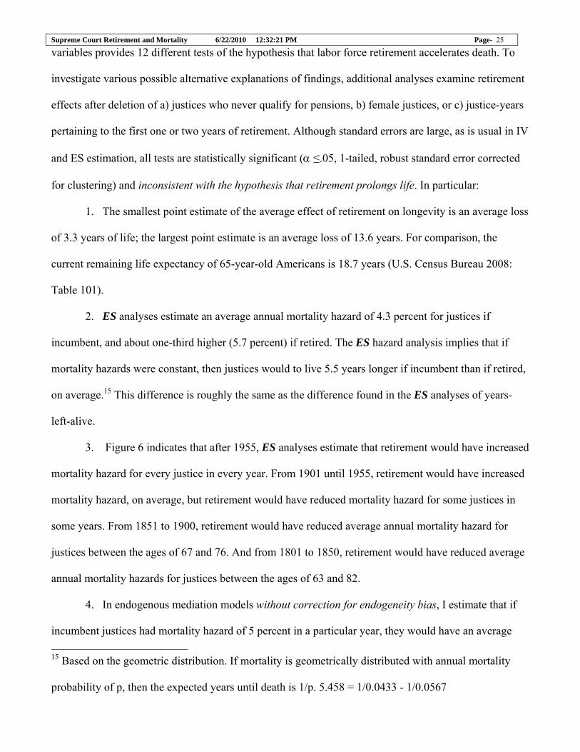
variables provides 12 different tests of the hypothesis that labor force retirement accelerates death. To
investigate various possible alternative explanations of findings, additional analyses examine retirement
effects after deletion of a) justices who never qualify for pensions, b) female justices, or c) justice-years
pertaining to the first one or two years of retirement. Although standard errors are large, as is usual in IV
and ES estimation, all tests are statistically significant (α ≤.05, 1-tailed, robust standard error corrected
for clustering) and inconsistent with the hypothesis that retirement prolongs life. In particular:
1. The smallest point estimate of the average effect of retirement on longevity is an average loss
of 3.3 years of life; the largest point estimate is an average loss of 13.6 years. For comparison, the
current remaining life expectancy of 65-year-old Americans is 18.7 years (U.S. Census Bureau 2008:
Table 101).
2. ES analyses estimate an average annual mortality hazard of 4.3 percent for justices if
incumbent, and about one-third higher (5.7 percent) if retired. The ES hazard analysis implies that if
mortality hazards were constant, then justices would to live 5.5 years longer if incumbent than if retired,
on average.15 This difference is roughly the same as the difference found in the ES analyses of years-
left-alive.
3. Figure 6 indicates that after 1955, ES analyses estimate that retirement would have increased
mortality hazard for every justice in every year. From 1901 until 1955, retirement would have increased
mortality hazard, on average, but retirement would have reduced mortality hazard for some justices in
some years. From 1851 to 1900, retirement would have reduced average annual mortality hazard for
justices between the ages of 67 and 76. And from 1801 to 1850, retirement would have reduced average
annual mortality hazards for justices between the ages of 63 and 82.
4. In endogenous mediation models without correction for endogeneity bias, I estimate that if
incumbent justices had mortality hazard of 5 percent in a particular year, they would have an average 15 Based on the geometric distribution. If mortality is geometrically distributed with annual mortality
probability of p, then the expected years until death is 1/p. 5.458 = 1/0.0433 - 1/0.0567

Supreme Court Retirement and Mortality 6/22/2010 12:32:21 PM Page- 26
hazard of more than 12 percent if they were retired in that year, other things equal. In models with IV
correction for endogeneity bias, if justices had a 5 percent mortality hazard if incumbent, then
retirement would raise that average hazard to more than 18 percent.16
In short, results are consistent with the hypothesis that, on average, voluntary retirement
substantially accelerates death of Supreme Court justices. If justices do indeed lengthen their lives by
working well into old age, then perhaps they are quite rational to eschew retirement, even if it brings a
generous pension.
VI. A CAUTIOUS CONCLUSION
Have these analyses neglected some exogenous variable that both causes retirement and
accelerates mortality? I hope not, but neglected variables are always possible. For example, readers have
suggested Presidential political party as possible confounding omitted variables. Stolzenberg and
Lindgren (forthcoming) do use similar data and methods to consider the effect of Presidential political
party on the timing of retirement from the Supreme Court, but, regardless of the effect of Presidential
16 For comparison, a recent study finds that smoking two or more packs of cigarettes a day (compared to
never smoking) would raise nonsmokers with a 5 percent mortality hazard to a 15.8 percent hazard. That
smoking effect is about midway between our instrumented and uninstrumented probit estimates of the
effect of retirement on one-year mortality hazard. So, even the smallest of the IV point estimates of
hazard effects can be characterized as comparable to the one-year mortality hazard effects of heavy
smoking. Of course, length of exposure matters too: smoking typically starts much earlier than
retirement, so lifetime effects of smoking would be much greater than lifetime effects of retirement,
even if the annual hazard rate effects of smoking and retirement were identical. Computed from Rogers
Hummer Krueger and Pampel (2005: 272), who report that the largest estimated logistic regression
coefficient for a dummy variable for smoking two or more packages of cigarettes a day, compared to
never having smoked, is 1.274.
Supreme Court Retirement and Mortality 6/22/2010 12:32:21 PM Page- 27
party on resignations, I am aware of no suggestion anywhere that the political party of the U.S. President
could directly affect the mortality hazard of individual Supreme Court justices.17 Family caregiving
responsibilities is also cited as a possible omitted variable, because other research reports that workers
sometimes retire to care for sick or disabled relatives (Raymo and Sweeney 2006) and care-giving is
found to reduce the health of care-givers (Reinhard and Horwitz 1995). But the care-givers described in
that research are mostly middle aged women with modest financial resources, demographically and
economically dissimilar to the mostly-male, highly educated, and well-paid individuals who are the past
and present justices of the Supreme Court.18 So it seems improbable, at best, that for Supreme Court
17 A reader asks for this paper “to convince readers why voluntary retirement is a rational decision at
all.” However, this paper is an analysis of an effect of retirement on mortality, not an examination of the
causes of retirement. Using similar data, Stolzenberg and Lindgren (2010) examine determinants of
retirement and death in office by Supreme Court justices.
18 Available information indicates that only one Supreme Court justice has cited care-giving as a reason
for retirement (Sandra Day O’Connor). But Justice O’Connor has placed her husband in a nursing
facility, where he is attended by professional caregivers (Zernike 2007). Further, it is impossible to
know the correspondence between O’Connor’s actual and stated reasons for retirement, and it is difficult
to know what effect, if any, her caregiving responsibilities might have on her mortality, as she remains
alive at this writing. In addition, Supreme Court justices are well-paid, so there is reason to believe that
they could buy caregiver services in place of their own labor, as Justice O’Connor has done. And,
further yet, evidence suggests that Supreme Court justices differ markedly from most contemporary
caregivers: According to a 1997 report (National Alliance for Caregiving and AARP 1997: p. 10),
caregivers are disproportionately female (74 percent), less than 50 years of age (64 percent), have low
household income (median $35000), and lacking professional or graduate education (91 percent). In
short, almost everything that is known about caregiving effects on caregivers applies to a population
segment that is very dissimilar to Supreme Court justices. Finally, the paper now reports that analyses

Supreme Court Retirement and Mortality 6/22/2010 12:32:21 PM Page- 28
justices, the need to perform unpaid family health care work explains the observed association between
justices’ mortality hazard and retirement. In brief, political circumstances and family health care
responsibilities do not seem to be omitted variables that rob our analyses of internal validity.
And there are the usual questions of external validity. Supreme Court data appear to solve
important measurement problems that afflict most other retirement and mortality data, but small
numbers always require caution. Further, Supreme Court justices are not average labor force
participants. Nor is work at the Court comparable to work at construction sites, high schools, coal mines,
or grocery stores, to name just a few places where people work. These and other limitations should be
considered seriously. At best, our findings suggest general patterns in certain other population segments.
For example, Supreme Court justices may resemble others characterized by very high achievement, who
hold jobs with high employment security, high job autonomy, pleasant working conditions, low work-
related physical demands, and high levels of work satisfaction. Although unusual, such persons are a
socially and economically important segment of the working population. Studies suggest that such
workers tend to retire later from the labor force than those who are not so characterized (see Raymo,
Warren, Sweeney, Hauser, and Ho 2008; Raymo and Sweeney 2006; Hayward, Grady, Hardy and
Sommers 1989). It seems reasonable to hypothesize that these talented workers who like to work at their
very good jobs may well react to retirement in much the same way as Supreme Court justices.
Obviously, more data would be needed before generalizing to larger population segments.
As we await that data, our results are added to analyses of other, sometimes larger, portions of
the population that find negative effects of retirement on subsequent health and longevity. Much of what
is known about work and employment effects on health and longevity has been discovered or tested on
seemingly unusual population subgroups, including civil servants in England (Stansfeld et al 1995),
residents of Alameda County, California (Camacho et al 1991), and the Wisconsin high school
were repeated after omitting Justice O’Connor and Justice Ginsburg, with no consequent change in
findings and virtually no change in estimates.

Supreme Court Retirement and Mortality 6/22/2010 12:32:21 PM Page- 29
graduating class of 1957 (Marks and Shinberg 1997). Finally, Preston (1977:171) aptly notes that low
mortality among “elderly leadership groups such as union leaders, Supreme Court justices, and
Communist Party officials” contributes to their grip on power, thereby making their longevity more
consequential than their small numbers might suggest. How interesting, then, that analyses reported here
suggest that, at least for U.S Supreme Court justices, the tenacious grip on power seems to contribute to
longevity, even as longevity prolongs their hold on high office.

Supreme Court Retirement and Mortality 6/22/2010 12:32:21 PM Page- 30
REFERENCES
Amemiya, T. 1985. Advanced econometrics. Cambridge, Mass.: Harvard University Press.
American Heritage. 1996. The American Heritage Dictionary of the English Language, Third Edition 1996
Boston: Houghton Mifflin.
Anderson, Kathryn H. 1985 The effect of mandatory retirement on mortality Journal of Economics and Business
37: 81-88
Ashenfelter, Orley and David Card 2002 Did the Elimination of Mandatory Retirement Affect Faculty
Retirement? The American Economic Review, Vol. 92, No. 4 (Sep., 2002), pp. 957-980
Berkman, Lisa F. 2000 “Social Integration, Social Networks, Social Support, and Health,” in Lisa F. Berkman and
Ichiro Kawachi (Eds.), Social Epidemiology (New York: Oxford University Press, 2000).
Berkman, Lisa F., and S. Leonard Syme, “Social Networks, Host Resistance, and Mortality: A Nine-Year Follow-
up Study of Alameda County Residents,” American Journal of Epidemiology 109 (June 1979), 186–204.
Binder, David A. 1983. On the Variances of Asymptotically Normal Estimators from Complex Surveys.
International Statistical Review 51: 279-292.
Blazer, Dan G. “Social Support and Mortality in an Elderly Community Population,” American Journal of
Epidemiology 115 (May 1982), 684–694
Bortz, W. M. II. 1984. The Disuse Syndrome. West. J. Med. 141(5):691-94
Bound, John 1991 “Self-Reported Versus Objective Measures of Health in Retirement Models” The Journal of
Human Resources, 26: 106-138
Buchner DM, Beresford SAA, Larson EB, LaCroix AZ, Wagner EH. Effects of physical activity on health status
in older adults II: Intervention Studies. Annual Review of Public Health. 1992. 13:469-488.
Calabresi, Steven G., and Lindgren, James. 2006a. “Term Limits for the Supreme Court: Life Tenure
Reconsidered.” Harvard Journal of Law and Public Policy 29: 770-877.
Camacho, T. C., Roberts, R. E., Lazarus, N. B., Kaplan, G. A., Cohen, R. D. 1991. Physical activity and
depression: Evidence from the Alameda County Study. Am. J. Epidemiol. 134(2):220-31
Cameron, John R. 2003. “Longevity Is the Most Appropriate Measure of Health Effects of Radiation” Radiology
229:14–15

Supreme Court Retirement and Mortality 6/22/2010 12:32:21 PM Page- 31
Cohen, Sheldon, W. J. Doyle, D. P. Skoner, B. S. Rabin, and J. M. Gwaltney, “Social Ties and Susceptibility to
the Common Cold.” Journal of the American Medical Association 277 (June 1997),1940–1944.
Colantonio, Angela, Stanislav V. Kasl, Adrian M. Ostfeld, and Lisa F. Berkman, “Psychosocial Predictors of
Stroke Outcome in an Elderly Population,” Journal of Gerontology 48:5 (1993), 261–268.
Crimmins, Eileen M., Mark D. Hayward, and Yasuhiko Saito, “Changing mortality and morbidity rates and the
health status and life expectancy of the older population.” Demography 31 (1994) pp. 119-175.
Farmer, M. E., Locke, B. Z., Moscicki, E. K., Dannenberg, A. L., Larson, D. B., et al. 1988. Physical activity and
depressive symptoms: The NHANES I epidemiologic follow-up study. Am. J. Epidemiol. 128:1340--51
Feng, Ziding, Dale Mclerran and James Grizzle 1998 “A Comparison of Statistical Methods for Clustered Data
Analysis with Gaussian Error” Statistics In Medicine Volume 15 Issue 16, Pages 1793 – 1806 Published
Online: 4 Dec 1998
Field, C.A. and A. H. Welsh 2007 “Bootstrapping clustered data” Journal of the Royal Statistical Society: Series
B (Statistical Methodology) Volume 69 Issue 3, Pages 369 – 390 Published Online: 22 May 2007
Fries, James F. 2005 “The Compression of Morbidity” The Milbank Quarterly 83 (4) , 801–823
Garrow, David J. 2000. “Mental Decrepitude on the U.S. Supreme Court: The Historical Case for a 28th
Amendment.” University of Chicago Law Review 67: 995.
Gerdtham UG, M Johannesson 2003 “A note on the effect of unemployment on mortality” J Health Econ. 2003
May;22(3):505-18
Gokhale, Jagadeesh 2004 “Mandatory Retirement Age Rules: Is It Time To Re-evaluate?” Testimony before the
U.S. Senate Special Committee on Aging Washington D.C. 20510 September 9, 2004
Gould, Lewis L.. 2000 "Moody, William Henry"; http://www.anb.org/articles/06/06-00447.html; Oxford
University Press: American National Biography Online Feb. 2000. Access Date: Mon Jun 29 01:04:35
CDT 2009
Gustman, Alan L. and Thomas L. Steinmeier 2001. “Retirement Outcomes in the Health and Retirement Study”
National Bureau for Economic Research. Research Paper No. 7588. Revised, September, 2001.
Handwerker, Elizabeth W. 2007. "Nixing the Notch: The Effects of the Social Security Notch on Overall
Incomes, Labor Supply, and Mortality in Retirement." Working paper. Washington, D.C.: U.S. Bureau of
Labor Statistics.

Supreme Court Retirement and Mortality 6/22/2010 12:32:21 PM Page- 32
Hjorth, Urban 1980 “A Reliability Distribution with Increasing, Decreasing, Constant and Bathtub-Shaped Failure
Rates” Technometrics, 22: 99-107
House, James S., Karl R. Landis, and Debra Umberson, “Social Relationships and Health,” Science 241 (July
1988), 540–545.
Idler, Ellen L. and Yael Benyamini 1997 Self-Rated Health and Mortality: A Review of Twenty-Seven
Community Studies Journal of Health and Social Behavior, 38: 21-37
Korpelainen, Helena. 2000 “Fitness, Reproduction and Longevity among European Aristocratic and Rural Finnish
Families in the 1700s and 1800s.” Proceedings of the Royal Society: Biological Sciences. Vol. 267, No.
1454, pp. 1765-1770
Leahey, Erin 2005 “Alphas and Asterisks: The Development of Statistical Significance Testing Standards in
Sociology” Social Forces 84:1-24.
Linn, M., R. Sandifer, and S. Stein 1985 “Effects of unemployment on mental and physical health”. Am J Public
Health. 75(5): 502–506
Litwin, Howard 2007 “Does early retirement lead to longer life ?”Ageing & Society 27, 2007, 739–754.
Lochner, Lance and Enrico Moretti 2004 “The Effect of Education on Crime: Evidence from Prison Inmates,
Arrests, and Self-Reports” The American Economic Review, Vol. 94, No. 1 (Mar., 2004), pp. 155-189
Manton, K. G, et. Al., “Time varying covariates of human mortality and aging: Multidimensional generalizations
of the Gompertz.” Journal of Gerontology: Biological Sciences 49:B169-B190.
Manton, K. G. and Stallard, E., “Heterogeneity and its Effect on Mortality Measurement” Chapter 12 in
Methodologies for the Collection and Analysis of Mortality Data. International Union for the Scientific
Study of Population, Vallin J, Pollard JH, Heligman L, Eds. 1984. Ordina Editions
http://www.cds.duke.edu/publications/DocLib/cds_1080.pdf
Mare, Robert D. and Christopher Winship. 1988. "Endogenous Switching Regression Models for the Causes and
Effects of Discrete Variables." Pp. 132-160 in Common Problems/Proper Solutions: Avoiding Error in
Quantitative Research, edited by J. S. Long. Newbury Park, CA: Sage.
Marks N.F. and D.S. Shinberg 1997 Socioeconomic differences in hysterectomy: the Wisconsin Longitudinal
Study. American Journal of Public Health. September; 87(9): 1507–1514.

Supreme Court Retirement and Mortality 6/22/2010 12:32:21 PM Page- 33
Marmot, Michael and Richard G. Wilkinson (eds.) 1999. Social Determinants of Health. Oxford: Oxford
University Press.
McCullagh, Peter 2000 “Resampling and Exchangeable Arrays” Bernoulli, Vol. 6, No. 2 (Apr., 2000), pp. 285-
301
McMahan, C. A.; John K. Folger; Stephen W. Fotis 1956 Retirement and Length of Life Social Forces, 34: 234-
238.
Mein G, P Martikainen, H Hemingway, S Stansfeld, M Marmot 2003 “Is retirement good or bad for mental and
physical health functioning? Whitehall II longitudinal study of civil servants” J Epidemiol Community
Health 2003;57:46–49
Morris, Joan K, Derek G Cook and A Gerald Shaper 1994 “Loss of employment and mortality” BMJ
308:1135-1139”
Munch, J. R. and Svarer, M. 2005. Mortality and socio-economic differences in Denmark: a competing risks
proportional hazard model. Economics and Human Biology, 3, 1, 17–32.
National Alliance for Caregiving and AARP. 1997. Family Caregiving in the US: Findings from a
national survey. Washington, DC: National Alliance for Caregiving & AARP
Olshansky, S. Jay, Bruce A. Carnes, Jacob Brody 2002 “A Biodemographic Interpretation of Life Span”
Population and Development Review, Vol. 28, No. 3, (Sep., 2002), pp. 501-513
Parsons, Donald O. 1980b. "Racial Trends in Male Labor Force Participation." American Economic Review,
70:911-920.
Parsons, Donald O. 1982a. "The Male Labor Force Participation Decision: Health, Reported Health, and
Economic Incentives." Economica, 49:81-91.
Parsons, Donald O. 1980a. "The Decline of Male Labor Force Participation." Journal of Political Economy,
88:117-134.
Peter R ; Siegrist J ; Hallqvist J ; Reuterwall C ; Theorell T .2002 . Psychosocial work environment and
myocardial infarction: improving risk estimation by combining two complementary job stress models in
the SHEEP Study. J Epidemiol Community Health (Journal of epidemiology and community health.)
2002 Apr; 56(4): 294-300

Supreme Court Retirement and Mortality 6/22/2010 12:32:21 PM Page- 34
Polivka, Anna and Jennifer Rothgeb 1993 “Redesigning the CPS Questionnaire” Monthly Labor Review 116: 10-
28.
Putnam, Robert D., Bowling Alone: The Collapse and Revival of American Community (New York: Simon &
Schuster, 2000).
Quandt R. 1972. “A new approach to estimating switching regression” . Journal of the American Statistical
Association 1972; 67: 306-310.
Raymo, James M. and Megan M. Sweeney 2006 “Work–Family Conflict and Retirement Preferences” Journal Of
Gerontology: Social Sciences 61B: S161–S169
Raymo, James M., John R. Warren, Megan M. Sweeney, Robert M. Hauser, and Jeong-Hwa Ho 2008 “Mid-life
Work Experiences and First Retirement” CDE Working Paper No. 2008-14. Madison, Wisconsin: Center
for Demography and Ecology, University of Wisconsin-Madison.
Redelmeier, Donald A and Sheldon M Singh 2001a “Longevity of screenwriters who win an academy award: a
longitudinal study” BMJ 323:1491-1496
Redelmeier, Donald A and Sheldon M Singh 2001b. Survival of academy award winning actors and actresses.
Ann Intern Med 2001;134:955-62.
Reinhard Susan C. and Allan V. Horwitz 1995 “Caregiver Burden: Differentiating the Content and
Consequences of Family Caregiving” Journal of Marriage and Family, 57: 741-750.
Reno, Virginia. 1971. "Why Men Stop Working at or before Age Sixty-five." Social Security Bulletin 34:3-16.
Rogers, Richard G., Robert A. Hummer, Patrick M. Krueger and Fred C. Pampel 2005 “Mortality Attributable to
Cigarette Smoking in the United States” Population and Development Review 31, No. 2 (Jun., 2005), pp.
259-292
Rones, Philip 1985 “Using the CPS to track retirement trends among older men.” Monthly Labor Review 108: 46-
49.
Schwab, Karen. 1974. "Early Labor Force Withdrawal of Men: Participants and Non-participants Aged 58-63."
Social Security Bulletin 37:24-38.

Supreme Court Retirement and Mortality 6/22/2010 12:32:21 PM Page- 35
Seeman, Teresa E., George Kaplan, Lisa Knudson, Richard Cohen, and Jack Guralnik, “Social Network Ties and
Mortality among the Elderly in the Alameda County Study,” American Journal of Epidemiology 126
(1987), 714–723.
Shang, Baoping and Dana Goldman 2008 “Does age or life expectancy better predict health care expenditures?”
Health Economics 17: 487-501
Sherman, Sally R. 1985. "Reported Reasons Retired Workers Left Their Last Job: Findings from the New
Beneficiary Survey." Social Security Bulletin 48:22-30.
Sickles, Robin, and Paul Taubman. 1986. "An Analysis of the Health and Retirement Status of the Elderly."
Econometrica 54:1339-56.
Siegrist, J. R. Peter, P. Cremer, D. Seidel. 1997. “Chronic work stress is associated with atherogenic lipids and
elevated fibrinogen in middle-aged men.” Journal of Internal Medicine. 242: 149-56.
Society of Actuaries. 1992. “Transactions of Society of Actuaries: 1991-92 Reports: Report of the Retirement
Plans Experience Committee: Mortality among members of uninsured pension systems”
Sorokin, Pitirim 1925 “Monarchs and Rulers: A Comparative Statistical Study” Social Forces Vol. 4, No. 1
(Sep., 1925), pp. 22-35
Stansfeld, Stephen, Amanda Feeney, Jenny Head, Robert Canner, Fiona North, Michael Marmot 1995 “Sickness
Absence for Psychiatric Illness: The Whitehall II” Social Science and Medicine 40 (2, Jan), 189-197
Stolzenberg Ross M. 2006 Multiple Regression Analysis. Chicago: The University of Chicago
Tsai, Shan, Judy Wendt, Robin Donnelly, Geert de Jong, and Farah Ahmed. 2005. “Age at retirement and long
term survival of an industrial population: prospective cohort study” British Medical Journal October 29;
331(7523): 995
U.S. Census Bureau, Statistical Abstract of the United States: 2008 (127th Edition) Washington, DC, 2007
Voss, M., Nylen, L., Floderus, B., Diderichsen, F., Terry, P. D. (2004). Unemployment and Early Cause-Specific
Mortality: A Study Based on the Swedish Twin Registry. Am. J. Public Health 94: 2155-2161
Wagner EH, LaCroix AZ, Buchner DM, Larson EB. Effects of physical activity on health status in older adults I:
observational studies. Annual Review of Public health. 1992:(13):145-68.

Supreme Court Retirement and Mortality 6/22/2010 12:32:21 PM Page- 36
Waldron, Hilary 2002 “Do Early Retirees Die Early? Evidence from Three Independent Data Sets” ORES
Working Paper Series,No. 97, Social Security Administration, Office of Policy, Office of Research,
Evaluation, and Statistics.
Waldron, Hilary. 2001. Links Between Early Retirement and Mortality. ORES Working Paper Series,No. 93,
Social Security Administration, Office of Policy, Office of Research, Evaluation, and Statistics. August.
Williams, Juan 1990 “The Thurgood Marshall Nobody Knows” Ebony May 1, 1990.
Wooldridge, Jeffrey M. 2001 Econometric Analysis of Cross Section and Panel Data. Cambridge, MA: The MIT
Press.
Yoon, Albert. 2006. “Pensions, Politics, and Judicial Tenure, An Empirical Study of Federal Judges, 1869-2002.”
American Law and Economics Review 8: 143-180.
Zernike, Kate 2007. New York Times, November 18, 2007 “Love in the Time of Dementia”
Zuckerman, Diana M., Stanislav V. Kasl, and Adrian M. Ostfeld, “Psychosocial Predictors of Mortality among
the Elderly Poor: The Role of Religion, Well-Being and Social Contacts,” American Journal of
Epidemiology 119 (March 1984), 410–123.

Supreme Court Retirement and Mortality 6/22/2010 12:32:21 PM Page- 37
Table 1 – Twelve Analyses of Retirement Effects on Mortality Hazard and Years-
left-alive
Identification and Estimation Methods Dependent Variable
Endogeneity Ignored
Instrumental Variables
Endogenous Switching
Years-left-alive
Model 1 1a Regression 1b Regression* 1c ANCOVA** 1d Tobit
Model 3 3a IVRegression 3b IVRegression* 3c IVTobit
Model 5 5a ES Regression 5b ES Regression*
Mortality Hazard
Model 2 Probit
Model 4 IV Probit
Model 6 ES Probit
Note: *To avoid negative estimates of years-left-alive, regressions are estimated with the following probit transformation of years-left-alive: Where Y is years-left-alive, Ψ is the transformed value of Y, Φ is the Normal cumulative distribution function, and Φ−1 is the inverse Normal cumulative distribution function, Ψ = Φ−1((Y+0.5)/50). For comparison purposes only, those regressions are also estimated with no transformation of remaining length of life. **Analysis of Covariance with probit transformation of years-left-alive; these are separate analyses for retired and incumbent justice years.

Supreme Court Retirement and Mortality 6/22/2010 12:32:21 PM Page- 38
Table 2a Descriptive Statistics for Discrete Time Event History Data, 1801-2006
Variable N Justice-
Years Mean Standard Deviation
Mini- mum
Maxi- mum
Year 2252 1911.467 57.66898 1801 2006 Age 2252 65.2873 10.55461 33 96 Tenure 2252 12.26643 8.387604 1 37 Qualified-for-pension 2252 .2801954 .4491943 0 1 Qualified-for-pension if not retired 1825 .2334247 .4231261 0 1 Retired 2252 .1896092 .3920789 0 1 Years-left-alive 2091 b 12.97131 9.359188 0 42 Age resigned from Court, if resigned 1297 72.54625 10.50579 47 90 Notes: aExcludes 135 justice-years for justices serving on Court in 2006. bExcludes 161 justice-years for justices serving on court in 2006, and the one live former justice in 2006, Sandra Day O’Connor. Table 2b- Historical Descriptive statistics: Characteristics of Former Supreme Court Justices in their Final Year on the Court, by Vitality at End of Service, 1789-2006 Former Justices Current Variable Name and Sta- All All Died in Justices Brief Description tistic Justices Former Office Retired 2006 n except Future Longevity n 110 101 49 52 9 Year Mean 1909.5 1900.9 1880.2 1920.4 2006 (Calendar Year) S.D. 62.82 58.21 48.18 60.51 0 Min 1793 1793 1798 1793 2006 Max 2006 2006 2005 2006 2006 Age Mean 69.58 69.85 68.82 70.83 66.56 (Justice’s Age in Years) S.D. 9.691 9.631 8.381 10.67 10.44 Min 48 48 48 48 51 Max 91 91 87 91 86 Tenure Mean 16.15 16.34 16.67 16.02 14 (Justice’s years of service S.D. 9.84 9.896 9.831 10.04 9.46 on the Supreme Court) Min 0 0 2 0 0 Max 36 36 34 36 31 Pension qualified Mean 0.5182 0.5050 0.3061 0.6923 0.6667 (dummy) S.D. 0.502 0.5025 0.4657 0.466 0.5000 Future Longevity n 100 100 49 51 n/a (Years between current Mean 4.35 4.35 0 8.529 n/a year and year of S.D. 7.258 7.258 0 8.242 n/a Justice’s death; n/a for Min 0 0 0 0 n/a justices now alive) Max 34 34 0 34 n/a Notes: At this time (June, 2006), except for Sandra Day O'Connor, all former justices of the Supreme Court are deceased. Two individuals were appointed to the Supreme Court two times: John Rutledge retired in 1791 and 1795. Charles Evans Hughes retired in 1916 and 1941.

Supreme Court Retirement and Mortality 6/22/2010 12:32:21 PM Page- 39
Table 3 – Robust, Cluster-Corrected Standard Errors and Test Statistics for First
Stage Regression and Probit Analyses of Retired on Exogenous Variables Regression Analysis Probit Analysis Independent variable Coefficient
Standard Error t Coefficient
Standard Error Z
Qualified-for-pension
.1528307 .0185742 8.23 .230499 .1259244 1.83
Age -.0231956 .0055049 -4.21 -.0691558 .0729478 -0.95 Age2 .0005687 .0000404 14.07 .0015023 .0005143 2.92 Age3 -3.61 x 10⁻⁶ 1.36 x 10⁻⁷ -26.57 Year1788 -.002061 .0005303 -3.89 .005611 .0010305 5.44 Year17882 9.98 x 10⁻⁶ 2.23 x 10⁻⁶ 4.48 Tenure -.0098628 .0025242 -3.91 -.0967758 .0081613 -11.86 Tenure2 .0002073 .0000733 2.83 Constant .306169 .1710694 1.79 -3.117741 2.582586 -1.21 N justice-years 1971 1971 R2 or Psueudo R2 0.5603 0.4366 F or Ln(likelihood)
F (8,1962) = 312.52 Ln(likelihood)= -505.261
Notes: The dependent variable in both of these analyses is the dummy variable retired. n for these analyses identical to n’s for IV analyses in Table 4.
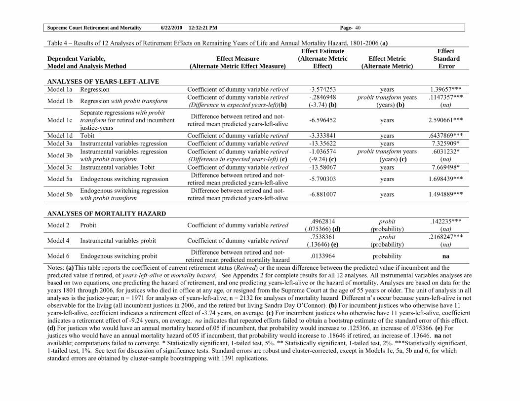
Supreme Court Retirement and Mortality 6/22/2010 12:32:21 PM Page- 40
Table 4 – Results of 12 Analyses of Retirement Effects on Remaining Years of Life and Annual Mortality Hazard, 1801-2006 (a)
Dependent Variable, Model and Analysis Method
Effect Measure (Alternate Metric Effect Measure)
Effect Estimate (Alternate Metric
Effect) Effect Metric
(Alternate Metric)
Effect Standard
Error ANALYSES OF YEARS-LEFT-ALIVE Model 1a Regression Coefficient of dummy variable retired -3.574253 years 1.39657***
Model 1b Regression with probit transform Coefficient of dummy variable retired(Difference in expected years-left)(b)
-.2846948 (-3.74) (b)
probit transform years (years) (b)
.1147357*** (na)
Model 1c Separate regressions with probit transform for retired and incumbent justice-years
Difference between retired and not-retired mean predicted years-left-alive -6.596452 years 2.590661***
Model 1d Tobit Coefficient of dummy variable retired -3.333841 years .6437869*** Model 3a Instrumental variables regression Coefficient of dummy variable retired -13.35622 years 7.325909*
Model 3b Instrumental variables regression with probit transform
Coefficient of dummy variable retired(Difference in expected years-left) (c)
-1.036574 (-9.24) (c)
probit transform years (years) (c)
.6031232* (na)
Model 3c Instrumental variables Tobit Coefficient of dummy variable retired -13.58067 years 7.669498*
Model 5a Endogenous switching regression Difference between retired and not-retired mean predicted years-left-alive -5.790303 years 1.698439***
Model 5b Endogenous switching regression with probit transform
Difference between retired and not-retired mean predicted years-left-alive -6.881007 years 1.494889***
ANALYSES OF MORTALITY HAZARD
Model 2 Probit Coefficient of dummy variable retired .4962814 (.075366) (d)
probit (probability)
.142235*** (na)
Model 4 Instrumental variables probit Coefficient of dummy variable retired .7538361 (.13646) (e)
probit (probability)
.2168247*** (na)
Model 6 Endogenous switching probit Difference between retired and not-retired mean predicted mortality hazard .0133964 probability na
Notes: (a) This table reports the coefficient of current retirement status (Retired) or the mean difference between the predicted value if incumbent and the predicted value if retired, of years-left-alive or mortality hazard, . See Appendix 2 for complete results for all 12 analyses. All instrumental variables analyses are based on two equations, one predicting the hazard of retirement, and one predicting years-left-alive or the hazard of mortality. Analyses are based on data for the years 1801 through 2006, for justices who died in office at any age, or resigned from the Supreme Court at the age of 55 years or older. The unit of analysis in all analyses is the justice-year; n = 1971 for analyses of years-left-alive; n = 2132 for analyses of mortality hazard Different n’s occur because years-left-alive is not observable for the living (all incumbent justices in 2006, and the retired but living Sandra Day O’Connor). (b) For incumbent justices who otherwise have 11 years-left-alive, coefficient indicates a retirement effect of -3.74 years, on average. (c) For incumbent justices who otherwise have 11 years-left-alive, coefficient indicates a retirement effect of -9.24 years, on average. na indicates that repeated efforts failed to obtain a bootstrap estimate of the standard error of this effect. (d) For justices who would have an annual mortality hazard of.05 if incumbent, that probability would increase to .125366, an increase of .075366. (e) For justices who would have an annual mortality hazard of.05 if incumbent, that probability would increase to .18646 if retired, an increase of .13646. na not available; computations failed to converge. * Statistically significant, 1-tailed test, 5%. ** Statistically significant, 1-tailed test, 2%. ***Statistically significant, 1-tailed test, 1%. See text for discussion of significance tests. Standard errors are robust and cluster-corrected, except in Models 1c, 5a, 5b and 6, for which standard errors are obtained by cluster-sample bootstrapping with 1391 replications.

Supreme Court Retirement and Mortality 6/22/2010 12:32:21 PM Page- 41
Table 5 – Coefficient of Retired from IV Models Estimated from only Justices who became Pension-Eligible
Model Analysis Method N
justices N justice-
years Coefficient of Retired
Cluster Corrected Robust Standard Error
3b Instrumental variables regression with probit transform 50 1269 -1.089993 .378642***
3c Instrumental variables Tobit 50 1269 -10.4401 4.832908** 4 Instrumental variables probit 57 1411 .9069707 .2824573***
Notes: This table reproduces the analyses shown in corresponding lines of Table 4, after excluding justices who resigned or died in office before qualifying for pension benefits. See notes for Table 4. Standard errors are robust and cluster-corrected ** Statistically significant, 1-tailed test, 2%. ***Statistically significant, 1-tailed test, 1%.

Supreme Court Retirement and Mortality 6/22/2010 12:32:21 PM Page- 42
Appendix A1 – Simulation Analyses to Address the Question, Are IV Estimates of the Effect of an Endogenous Regressor Necessarily Weaker than Reduced Form Estimates?
A skeptical reader proposes that the estimated effect of retired on mortality must be weaker when
estimated with IV analyses than when estimated in analyses that ignore endogeneity. This appendix uses
simulation to examine that concern by (see also general treatments that permit an entirely mathematical
approach, e.g. Amemiya 1985 and Wooldridge 2001). In a related matter, Lochner and Moretti (2004) show
mathematically that statistical significance levels for IV estimates can be higher than significance levels for
reduced form estimates.
The model represented in figure A1 is used to construct the simulation data. L is the observed dependent
variable of interest, analogous to longevity. R is an observed endogenous regressor, analogous to retirement. Z
is an observed exogenous variable that affects R directly, analogous to qualified for pension in our Supreme
Court analyses. Z affects L only indirectly, through its effect on R, thus making Z suitable for use as an
instrument for R. εRR and ε LL are exogenous disturbances. S is an exogenous variable that is unobservable by
the hypothetical data analyst. Thus, S is relegated to treatment as a component of disturbances εR and εL, and
thereby generates a correlation between them. The analysis depicted in Figure A2 ignores the endogeneity of R.
The effect of R on L in Figure A2 is estimated by ordinary least squares (OLS); Figure A2 is underidentified,
and OLS estimates of its parameters are biased. The analysis in Figure A3 uses Z as an instrument for R. Figure
A3 is just identified and effects are estimated by IV regression. The model is specified mathematically as
follows:
(A1) εRR ~ N0,1 (A2) εLL ~ N0,1 (A3) S ~ N0,1 (A4) Z ~ N0,1 (A5) Σ = I4 where I4 is the identity matrix of order 4 and Σ is the variance-covariance matrix of εRR, εLL, S, Z. (A6) εR = εRR + 0.5ΔS where Δ is a coefficient equal to 1 or -1. (A7) εL = εLL + ΩS where Ω is a coefficient equal to 1 or -1. (A8) R = Z + εR

Supreme Court Retirement and Mortality 6/22/2010 12:32:21 PM Page- 43
(A9) L = ΦR + εL where Φ is a coefficient equal to 1 or -1.
Equation (A10) is used to estimate by OLS the model of L shown in Figure A2. (A10) L̂ ols = β0 + β1 R
Equations (A11) and (A12) are used to estimate by IV regression the model shown in Figure A3. (A11) R̂ = π0 + π1 Z (A12) L̂ IV = α0 + α2 R̂
I estimate simulations under eight conditions corresponding to values of -1 or +1 for each coefficient Δ,
Ω, and Φ. Using Stata 9.2 (with a random number seed X075bcd151f123bb5159a55e5002286574 6ad), I
generate 100,000 replicates of εRR , ε LL , S, and Z, and then use OLS and IV (two stage least squares)
regression to fit the models indicated in Figures A1 and A2. Table A1 shows results. Although the skeptical
reader proposed that the IV estimates would be weaker than the OLS estimates of Φ, results show that in half
the simulations, the absolute size of the OLS estimate is smaller than the absolute size of the IV estimator.
Table A1 – Simulation Results, N=100,000 Each Design Parameter Estimate of Φ
Design Number Δ Ω Φ OLS IV
Larger Absolute Estimate
1 -1 -1 1 1.23 1.01 OLS 2 -1 -1 -1 -0.77 -0.99 IV 3 -1 1 1 0.78 1.00 IV 4 -1 1 -1 -1.22 -1.00 OLS 5 1 1 1 1.23 1.00 OLS 6 1 1 -1 -0.77 -1.00 IV 7 1 -1 1 0.78 1.01 IV 8 1 -1 -1 -1.22 -0.99 OLS

Supreme Court Retirement and Mortality 6/22/2010 12:32:21 PM Page- 44

Supreme Court Retirement and Mortality 6/22/2010 12:32:21 PM Page- 45
APPENDIX 2 COMPLETE ANALYSIS RESULTS FOR TABLE 4
>>>>INCLUDED FOR REVIEWERS, BUT NOT NECESSARILY FOR PUBLICATION<<<<
Model 1a -- OLS Regression of Years Left Alive, with Robust Standard Errors Corrected for Clustering Independent Variable Coefficient Robust S.E. t retired -3.574253 1.39657 -2.56 tenure -.2186793 .0706771 -3.09 year1788 .1025659 .0657349 1.56 year17882 .000191 .0002771 0.69 age -1.678824 .3520718 -4.77 age2 .0109136 .0028048 3.89 age*year1788 -16.50542 10.7429 -1.54 constant 75.7191 10.2454 7.39 N 1971 R2 0.4503 Notes: Estimated over all justice-years 1801-2006 for justices deceased by 2006 who did not retire before age 55. Standard errors are robust and corrected for clustering.
Model 1b -- OLS Regression of Probit-Transformed Years Left Alive, with Robust Standard Errors Corrected for Clustering Independent Variable Coefficient Robust S.E. t Age -.0772333 .0238676 -3.24 Age2 .0003088 .000177 1.74 Age3 6.13e-07 5.98e-07 1.02 year1788 .0010377 .004187 0.25 year17882 8.01e-06 .000016 0.50 tenure -.0017634 .0133526 -0.13 tenure2 -.0005205 .0003079 -1.69 retired -.2846948 .1147357 -2.48 Constant 2.695483 .6648214 4.05 N 1971 R2 .4115 Notes: Estimated over all justice-years 1801-2006 for justices deceased by 2006 who did not retire before age 55. Standard errors are robust and corrected for clustering.

Supreme Court Retirement and Mortality 6/22/2010 12:32:21 PM Page- 46
Model 1c -- Separate regressions of Probit-Transformed Years Left Alive for retired and incumbent justice-years Retired Justices Only Independent Variable Coefficient Robust S.E. t tenure -.0185406 .0075543 -2.45 year1788 .0151861 .0078526 1.93 year17882 -.0000121 .0000279 -0.44 age .08479 .1267269 0.67 age2 -.0005418 .0008467 -0.64 age*year1788 -1.421189 1.290685 -1.10 constant -4.633766 4.483483 -1.03 N 334 R2 0.2467 Notes: Estimated over all justice-years 1801-2006 for justices deceased by 2006 who did not retire before age 55. Standard errors are robust and corrected for clustering.
Incumbent Justices Only Independent Variable Coefficient Robust S.E. t tenure -.0162098 .0067212 -2.41 year1788 .0003398 .004854 0.07 year17882 .0000218 .0000212 1.03 age -.0706071 .0259633 -2.72 age2 .0003379 .0002459 1.37 age*year1788 -.3532584 .8616054 -0.41 constant 2.490507 .6571686 3.79 N 1637 R2 0.3696 Notes: Estimated over all justice-years 1801-2006 for justices deceased by 2006 who did not retire before age 55. Standard errors are robust and corrected for clustering.

Supreme Court Retirement and Mortality 6/22/2010 12:32:21 PM Page- 47
Model 1c -- Separate regressions of Years Left Alive for retired and incumbent justice-years Retired Justices Only Independent Variable Coefficient Robust S.E. t tenure -.1767526 .0845531 -2.09 year1788 .2012675 .1025484 1.96 year17882 -.0003024 .000309 -0.98 age .2642597 1.54243 0.17 age2 -.0017258 .0104017 -0.17 age*year1788 -14.23091 15.50226 -0.92 Constant -7.309449 54.63108 -0.13 N 334 R2 0.2632 Notes: Estimated over all justice-years 1801-2006 for justices deceased by 2006 who did not retire before age 55. Standard errors are robust and corrected for clustering.
Incumbent Justices Only Independent Variable Coefficient Robust S.E. t tenure -.2358315 .0937814 -2.51 year1788 .0701248 .0756628 0.93 year17882 .0003229 .0003019 1.07 age -1.610293 .3359931 -4.79 age2 .0103302 .0029666 3.48 age*year1788 -15.82976 12.32282 -1.28 Constant 75.08222 8.914693 8.42 N 1637 R2 0.4199 Notes: Estimated over all justice-years 1801-2006 for justices deceased by 2006 who did not retire before age 55. Standard errors are robust and corrected for clustering.
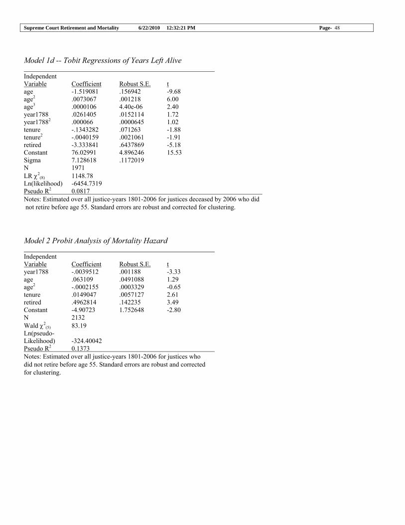
Supreme Court Retirement and Mortality 6/22/2010 12:32:21 PM Page- 48
Model 1d -- Tobit Regressions of Years Left Alive Independent Variable Coefficient Robust S.E. t age -1.519081 .156942 -9.68 age2 .0073067 .001218 6.00 age3 .0000106 4.40e-06 2.40 year1788 .0261405 .0152114 1.72 year17882 .000066 .0000645 1.02 tenure -.1343282 .071263 -1.88 tenure2 -.0040159 .0021061 -1.91 retired -3.333841 .6437869 -5.18 Constant 76.02991 4.896246 15.53 Sigma 7.128618 .1172019 N 1971 LR χ2
(8) 1148.78 Ln(likelihood) -6454.7319 Pseudo R2 0.0817 Notes: Estimated over all justice-years 1801-2006 for justices deceased by 2006 who did not retire before age 55. Standard errors are robust and corrected for clustering.
Model 2 Probit Analysis of Mortality Hazard Independent Variable Coefficient Robust S.E. t year1788 -.0039512 .001188 -3.33 age .063109 .0491088 1.29 age2 -.0002155 .0003329 -0.65 tenure .0149047 .0057127 2.61 retired .4962814 .142235 3.49 Constant -4.90723 1.752648 -2.80 N 2132 Wald χ2
(5) 83.19 Ln(pseudo- Likelihood) -324.40042 Pseudo R2 0.1373 Notes: Estimated over all justice-years 1801-2006 for justices who did not retire before age 55. Standard errors are robust and corrected for clustering.

Supreme Court Retirement and Mortality 6/22/2010 12:32:21 PM Page- 49
Model 3a – Regression of Years Left Alive First-stage regression of Retired Independent Variable Coefficient Robust S.E. t age -.0231956 .0055049 -4.21 age2 .0005687 .0000404 14.07 age3 -3.61e-06 1.36e-07 -26.57 year1788 -.002061 .0005303 -3.89 year17882 9.98e-06 2.23e-06 4.48 tenure -.0098628 .0025242 -3.91 tenure2 .0002073 .0000733 2.83 qual4pen .1528307 .0185742 8.23 Constant .306169 .1710694 1.79 N 1971 R2 0.5603 Notes: Estimated over all justice-years 1801-2006 for justices deceased by 2006 who did not retire before age 55. Standard errors are robust and corrected for clustering. Instrumental variables (2SLS) regression Independent Variable Coefficient Robust S.E. t retired -13.35622 7.325909 -1.82 age -1.914292 .4524699 -4.23 age2 .0144326 .0055055 2.62 age3 -.000024 .0000243 -0.99 year1788 .0123105 .0627544 0.20 year17882 .0001476 .0002517 0.59 tenure -.2095038 .1850819 -1.13 tenure2 -.0018258 .003969 -0.46 Constant 82.83009 12.20146 6.79 N 1971 R2 0.3661 Notes: Estimated over all justice-years 1801-2006 for justices deceased by 2006 who did not retire before age 55. Standard errors are robust and corrected for clustering.

Supreme Court Retirement and Mortality 6/22/2010 12:32:21 PM Page- 50
Model 3b -- IV Regression of Probit Transformed Years Left Alive
First-stage Regression of Retired Independent Variable Coefficient Robust S.E. t age -.0231956 .0055049 -4.21 age2 .0005687 .0000404 14.07 age3 -3.61e-06 1.36e-07 -26.57 year1788 -.002061 .0005303 -3.89 year17882 9.98e-06 2.23e-06 4.48 tenure -.0098628 .0025242 -3.91 tenure2 .0002073 .0000733 2.83 qual4pen .1528307 .0185742 8.23 Constant .306169 .1710694 1.79 N 1971 R2 0.5603 Notes: Estimated over all justice-years 1801-2006 for justices deceased by 2006 who did not retire before age 55. Standard errors are robust and corrected for clustering. Instrumental variables (2SLS) regression Independent Variable Coefficient Robust S.E. t retired -1.036574 .6031232 -1.72 age -.1018938 .0317218 -3.21 age2 .0007896 .0004223 1.87 age3 -1.89e-06 1.95e-06 -0.97 year1788 -.0001655 .0044944 -0.04 year17882 .0000153 .0000185 0.82 tenure -.0059157 .0140778 -0.42 tenure2 -.0004328 .0003397 -1.27 Constant 3.076704 .8184089 3.76 N 1971 R2 0.3354
Notes: Estimated over all justice-years 1801-2006 for justices deceased by 2006 who did not retire before age 55. Standard errors are robust and corrected for clustering.

Supreme Court Retirement and Mortality 6/22/2010 12:32:21 PM Page- 51
Model 3c Instrumental Variables Tobit Regressions of Years Left Alive Instrumental variables Tobit regression of Years left Alive Independent Variable Coefficient Robust S.E. t retired -13.58067 7.669498 -1.77 age -1.857586 .4564751 -4.07 age2 .0138752 .0056318 2.46 age3 -.0000235 .0000252 -0.93 year1788 .0096202 .0651035 0.15 year17882 .0001654 .0002628 0.63 tenure -.1920307 .1921549 -1.00 tenure2 -.0027865 .0042272 -0.66 Constant 81.30999 12.24022 6.64 N 1971 Wald χ2 (8) 373.53 Ln(pseudo- likelihood -6504.8751 Notes: Estimated over all justice-years 1801-2006 for justices deceased by 2006 who did not retire before age 55. Standard errors are robust and corrected for clustering. First-stage Probit Analysis of Retired Independent Variable Coefficient Robust S.E. t age -.0231956 .0183781 -1.26 age2 .0005687 .000168 3.39 age3 -3.61e-06 5.09e-07 -7.08 year1788 -.002061 .0012595 -1.64 year17882 9.98e-06 5.57e-06 1.79 tenure -.0098628 .0047287 -2.09 tenure2 .0002073 .0001231 1.68 qual4pen .1528307 .0565794 2.70 Constant .306169 .4996489 0.61 N 1971 Notes: Estimated over all justice-years 1801-2006 for justices deceased by 2006 who did not retire before age 55. Standard errors are robust and corrected for clustering.

Supreme Court Retirement and Mortality 6/22/2010 12:32:21 PM Page- 52
Model 4 Instrumental Variables Probit Analysis of Mortality Hazard
A. Probit Analysis of Mortality Hazard Independent Variable Coefficient Robust S.E. t retired .7538361 .2168247 3.48 year1788 -.0041319 .0011201 -3.69 age .0862405 .0536082 1.61 age2 -.0004365 .0003811 -1.15 tenure .0202197 .0074704 2.71 Constant -5.534755 1.884165 -2.94 N 2132 Wald χ2
(5) 89.57 Ln(pseudo- Likelihood) -332.88078 Notes: Estimated over all justice-years 1801-2006 for justices who did not retire before age 55. Standard errors are robust and corrected for clustering. B. First Stage Probit Analysis of Retired Independent Variable Coefficient Robust S.E. t year1788 -.0004743 .0010528 -0.45 year17882 2.01e-06 4.28e-06 0.47 age -.0296732 .0171831 -1.73 age2 .0006281 .0001588 3.95 age3 -3.71e-06 5.22e-07 -7.11 tenure -.0101764 .0046932 -2.17 tenure2 .00024 .0001304 1.84 qual4pen .1381422 .051353 2.69 Constant .4392054 .4753172 0.92

Supreme Court Retirement and Mortality 6/22/2010 12:32:21 PM Page- 53
Model 5a – Endogenous Switching Regression Analyses of Years Left Alive
First-stage Regression of Retired Independent Variable Coefficient Robust S.E. t qual4pen .230499 .1259244 1.83 age -.0691558 .0729478 -0.95 age2 .0015023 .0005143 2.92 year1788 .005611 .0010305 5.44 tenure -.0967758 .0081613 -11.86 Constant -3.117741 2.582586 -1.21 LR chi2(5) 783.18 Pseudo R2 0.4366 Log likelihood -505.261 N 1971 Notes: Estimated over all justice-years 1801-2006 for justices deceased by 2006 who did not retire before age 55. Standard errors are robust and corrected for clustering. Endogenous Switching Regression of Years Left Alive, Retired Only Independent Variable Coefficient Robust S.E. t age .6692842 1.600425 0.42 age2 -.0063831 .0098246 -0.65 year1788 .0081152 .0167509 0.48 tenure -.1543455 .0818264 -1.89 Constant -4.431863 64.57724 -0.07 Wald χ2
(4) 10.98 Ln( pseudo- likelihood -1556.475 N 1971 Uncensored N 334 Notes: Estimated over all justice-years 1801-2006 for justices deceased by 2006 who did not retire before age 55. Standard errors are robust and corrected for clustering.
Endogenous Switching Regression of Years Left Alive, Incumbent Only Independent Variable Coefficient Robust S.E. t age -1.89451 .4557748 -4.16 age2 .0117676 .0044845 2.62 year1788 .0466799 .017038 2.74 tenure -.2745009 .1324152 -2.07 Constant 84.64221 12.10133 6.99 N 1971 Wald χ2
(4) 343.86 Uncensored N 1637 Ln(pseudo- likelihood -6030.015 Notes: Estimated over all justice-years 1801-2006 for justices deceased by 2006 who did not retire before age 55. Standard errors are robust and corrected for clustering.

Supreme Court Retirement and Mortality 6/22/2010 12:32:21 PM Page- 54
Model 5b – Endogenous Switching Regression Analyses of Probit-Transformed Years Left Alive Endogenous Switching Regression of Probit Transformed Years Left Alive, Retired Only Independent Variable Coefficient Robust S.E. t age .0740601 .1462538 0.51 age2 -.000717 .0008651 -0.83 year1788 .000472 .0017244 0.27 tenure -.0115464 .0105761 -1.09 Constant -2.386027 6.16838 -0.39 N 1971 Uncensored N 334 Wald χ2
(4) 16.84 Ln(pseudo- likelihood -777.8706 Notes: Estimated over all justice-years 1801-2006 for justices deceased by 2006 who did not retire before age 55. Standard errors are robust and corrected for clustering. Endogenous Switching Regression of Probit Transformed Years Left Alive, Incumbent Only Independent Variable Coefficient Robust S.E. t age -.0748656 .0203591 -3.68 age2 .0003159 .0001846 1.71 year1788 .0029542 .0011001 2.69 tenure -.0132261 .0070124 -1.89 Constant 2.607436 .5710812 4.57 N 1971 Uncensored N 1637 Wald χ2
(4) 322.77 Ln(Pseudo- likelihood) -1769.277 Notes: Estimated over all justice-years 1801-2006 for justices deceased by 2006 who did not retire before age 55. Standard errors are robust and corrected for clustering.

Supreme Court Retirement and Mortality 6/22/2010 12:32:21 PM Page- 55
Model 6 Endogenous Switching Probit Analysis of Mortality Hazard A. First Stage Probit Analysis of Retired Independent Variable Coefficient Robust S.E. t qual4pen .2148681 .1238097 1.74 age -.0462563 .0734785 -0.63 age2 .0013982 .0005168 2.71 year1788 .0036605 .0009559 3.83 tenure -.1017056 .0081515 -12.48 Constant -3.918372 2.611989 -1.50 N 2132 LR χ2
(5) 796.54 Ln(like- lihood -527.21186 Pseudo R2 0.4303 Notes: Estimated over all justice-years 1801-2006 for justices who did not retire before age 55. Standard errors are robust and corrected for clustering. B. Probit Analysis of Mortality Hazard for Retired Only Independent Variable Coefficient Robust S.E. t age -.0608349 .1993165 -0.31 age2 .0006625 .0011915 0.56 year1788 -.0016844 .0022062 -0.76 tenure .013234 .019291 0.69 Constant -.6299868 8.359182 -0.08 N 2132 Censored N 1798 Wald χ2
(4) 15.24 Log likelihood -641.3718
Notes: Estimated over all justice-years 1801-2006 for justices who did not retire before age 55. Standard errors are robust and corrected for clustering. C. Analysis of Mortality Hazard for Incumbent Only Independent Variable Coefficient Robust S.E. t age .1172049 .1118509 1.05 age2 -.0005329 .0008795 -0.61 year1788 -.0042365 .0014241 -2.97 tenure .0058439 .0147427 0.40 Constant -6.850955 3.654688 -1.87 N 2132 Censored N 334 Wald χ2(4) 39.43 Log likelihood -735.6234 Notes: Estimated over all justice-years 1801-2006 for justices who did not retire before age 55. Standard errors are robust and corrected for clustering.