Prepared under Bureau of Ocean Energy Management Award Interagency No. M09PG00025, AK-09-05B

Demographic Composition and Behavior of Polar Bears Summering on Shore in Alaska

By Todd C. Atwood1, Elizabeth M. Peacock1, Melissa A. McKinney2, Kate Lillie3, Ryan R. Wilson4, and Susanne Miller4

1U.S. Geological Survey, Alaska Science Center, Anchorage, AK 2Department of Natural Resources and the Environment and Center for Environmental Sciences and Engineering, University of Connecticut, Storrs, CT 3Department of Wildland Resources, Utah State University, Logan, UT 4U.S. Fish and Wildlife Service, Anchorage, AK

Administrative Report

U.S. Department of the Interior U.S. Geological Survey

U.S. Department of the Interior SALLY JEWELL, Secretary

U.S. Geological Survey Suzette M. Kimball, Acting Director

U.S. Geological Survey, Reston, Virginia: 2015

Any use of trade names is for descriptive purposes only and does not imply endorsement by the U.S. Government

Suggested citation:

Atwood, T.C., Peacock, E.M., McKinney, M.A., Lillie, K., Wilson, R.R., and Miler, S., 2015, Demographic

composition and behavior of polar bears summering on shore in Alaska: U.S. Geological Survey Administrative

Report, 26 p.

iii

Contents

1.0 Executive Summary .............................................................................................................................................. 1

2.0 Introduction ........................................................................................................................................................... 2 3.0. Methods ............................................................................................................................................................... 3

3.1. Data Collection ................................................................................................................................................. 5 3.2. Demographic Composition, Relative Density, and Distribution ........................................................................ 5 3.3. Phenology of Land Use and Length of Stay ..................................................................................................... 6 3.4. Sea Ice Characteristics .................................................................................................................................... 6

3.5. Characterizing Nutritional Condition ................................................................................................................. 8 3.6. Analyses .......................................................................................................................................................... 8

4.0. Results ............................................................................................................................................................... 11 4.1. Demographic Composition and Relative Density ........................................................................................... 11 4.2. Distribution ..................................................................................................................................................... 12 4.3. Phenology of Land Use .................................................................................................................................. 15

4.4. Characterizing Nutritional Condition ............................................................................................................... 18 Discussion ................................................................................................................................................................ 18 Acknowledgments ..................................................................................................................................................... 21

References Cited ...................................................................................................................................................... 22

Figures

Figure 1. Map showing southern Beaufort Sea polar bear study area, Alaska, 1986–2013. ..................................... 4 Figure 2. Map showing spatial distribution of polar bears observed during fall aerial surveys along the coast and over barrier islands prior to the stocking of bowhead whale bone piles with remains from the subsistence harvest, Alaska, 2010–13 ...................................................................................................................................................... 13 Figure 3. Map showing spatial distribution of polar bears observed during fall aerial surveys along the coast and over barrier islands after the stocking of bowhead whale bone piles with remains from the subsistence harvest, Alaska, 2010–13 ...................................................................................................................................................... 14 Figure 4. Graph showing proportion of radiocollared adult female polar bears that spent ≥21 consecutive days on shore, Alaska, 1986–2013 ....................................................................................................................................... 15 Figure 5. Graph showing mean (and standard error) length of stay on shore relative to the length of the open-water season, defined as the time when the proportion of the continental shelf covered by >15% sea ice concentration decreases to ≤15%. ......................................................................................................................... 17

iv

Tables

Table 1. Description of sea ice variables used in the analysis of factors influencing the timing of arrival on shore, length of stay, and timing of departure back to sea ice by polar bears from the Southern Beaufort Sea subpopulation. ........................................................................................................................................................... 7 Table 2. Example of hypotheses and variables used in candidate regression models tested to predict the timing of arrival on shore, length of stay on shore, and departure from shore by adult female polar bears, 1986–2013. ....... 10 Table 3. Aerial transect (coastal and perpendicular segments) survey and total count data for Barter and Cross islands, distance surveyed, and relative density of polar bears observed on shore, 2010–2013. ............................ 11

Table 4. Demography of polar bears observed on shore during fall aerial surveys and island total counts, and captured on sea ice during spring, 2010–2013. ....................................................................................................... 12 Table 5. Response variables, explanatory variables, model rank, AICc value, and significant variables, with individual identity as a random effect for the top generalized additive mixed models. ............................................. 16 Table 6. Ranking of variables retained in top models of length of time spent on shore. ......................................... 16 Table 7. Ranking of variables retained in top models of date of departure from shore back to the sea ice. ........... 17

Conversion Factors

International System of Units to Inch/Pound

Multiply By To obtain

Length

kilometer (km) 0.6214 mile (mi)

meter (m) 3.281 foot (ft)

meter (m) 1.094 yard (yd)

Abbreviations and Acronyms

AIC Akaike information criteria

CRAWL Continuous-time correlated random walk

GIS Geographic information system

GPS Global positioning system

SB Southern Beaufort Sea

1

Demographic Composition and Behavior of Polar Bears Summering on Shore in Alaska

By Todd C. Atwood1, Elizabeth M. Peacock2, Melissa A. McKinney3, Kate Lillie4, Ryan R. Wilson4, and Susanne Miller4

1.0 Executive Summary

In the Arctic Ocean’s southern Beaufort Sea (SB), the length of the sea ice melt season (that is,

the period between the onset of sea ice break-up in summer and freeze-up in fall) has increased

substantially since the late 1990s. Historically, polar bears (Ursus maritimus) of the SB have remained

on the sea ice year-round (except during denning), but recent changes in the extent and phenology of sea

ice habitat have coincided with increased use of terrestrial habitat.

We characterized the demographic composition, spatial behavior, and nutritional condition of

polar bears spending summer on shore along Alaska’s northern coast to better understand the nexus

between rapid environmental change and increased use of terrestrial habitat. We found that the

proportion of the SB subpopulation coming ashore in summer and fall has doubled over time and the

sex and age class composition of polar bears on shore was similar to the composition of bears

encountered in our study area on the sea ice in spring. Moreover, we detected trends of earlier arrival on

shore, increased length of stay, and later departure back to sea ice, all of which were related to declines

in the availability of sea ice habitat over the continental shelf and changes to sea ice phenology.

Since the late 1990s, the duration of the open-water season in the SB increased by 36 days, and

the length of stay on shore increased by 25 days. While on shore, the distribution of polar bears was

influenced by the availability of scavenge subsidies in the form of subsistence-harvested bowhead whale

(Balaena mysticetus) remains aggregated at sites along the coast. Analyses of nutritional condition

suggests bears may derive a benefit from scavenging. The declining availability of sea ice habitat, the

lengthening melt season, and increased availability of human-provisioned resources are likely to result

in continued growing use of land. Increased residency on land is cause for concern given that, while

there, bears may be exposed to a greater array of risk factors including those associated with increased

human activities.

1U.S. Geological Survey.

2Department of Natural Resources and the Environment and Center for Environmental Sciences and

Engineering, University of Connecticut, Storrs. 3Department of Wildland Resources, Utah State University, Logan.

4U.S. Fish and Wildlife Service.

2

2.0 Introduction

Since at least the early 2000s, polar bears (Ursus maritimus) in the southern Beaufort Sea (SB)

subpopulation have been spending increased time on the coastal North Slope of Alaska between July

and October (Gleason and Rode, 2010). From 2000 to 2005, using coastal aerial surveys, Schliebe and

others (2008) observed between 3.7 and 8.0% (about 60–120 of 1,526; Regehr and others, 2006) of

polar bears on land during summer and fall. Although the percentage of the subpopulation estimated to

be coming ashore in the early 2000s was small, it did represent a change in behavior in that prior to

2000 extended use of land was considered rare (for example, Amstrup and others, 2000). This change in

polar bear ecology has relevance for human-bear interactions, subsistence harvest and defense kills, and

disturbance associated with existing and proposed land-based development (for example, National

Petroleum Reserve of Alaska, Arctic National Wildlife Refuge), Native Alaskan communities,

recreation, and tourism (for example, bear viewing in Kaktovik, Alaska). Increased use of terrestrial

habitat by SB polar bears also has the potential to impact, in new ways, the status of the entire

subpopulation by mediating exposure to risk factors associated with terrestrial ecosystems (for example,

novel disease agents, industrial pollutants). Accordingly, a characterization of the demography and

behavior of polar bears summering on shore is needed to help inform decisions regarding the

management (for example, industry permitting under the Endangered Species Act and Marine Mammal

Protection Act) of polar bears and population stressors (for example, Atwood and others, 2015) in a

rapidly changing environment.

In contrast to the SB subpopulation, 5 of the world’s 19 polar bear subpopulations (that is,

western Hudson Bay, southern Hudson Bay, Davis Strait, Baffin Bay, and Foxe Basin) spend significant

periods of time on land (1–5 months) when ice completely melts each summer (Obbard and others,

2010). In these seasonal-ice subpopulations (Amstrup and others, 2008), polar bears are largely in a

hypophagic condition (Hobson and Stirling, 1997; Hobson and others, 2009) while on shore, relying on

fat stores they obtain during the spring hyperphagic season when ringed seal (Phoca hispida) pups and

molting adults are most vulnerable to predation (Stirling and Øritsland, 1995). Generally, the seasonal-

ice subpopulations have been demographically productive (Taylor and others, 2005; Peacock and others,

2013; Stapleton and others, 2015), although an increase in the ice-free season was attributed to a

population decline in western Hudson Bay (WHB; Stirling and others, 1999; Regehr and others, 2007).

Similar to WHB, there have been measured declines in the body condition, productivity, survival, and

abundance of polar bears in the SB, and changes in these parameters have been linked directly and

indirectly to declining availability of sea ice habitat (Hunter and others, 2010; Regehr and others, 2010;

Rode and others, 2010; Bromaghin and others, 2015). However, studies of other subpopulations have

failed to identify links between habitat change and adverse population-level impacts (for example,

Peacock and others, 2013; Rode and others, 2014; Obbard and others, 2015; Stapleton and others,

2015). Geographic variation in productivity and exposure to risk factors may mediate differences in the

response of polar bears to declines in sea ice habitat.

3

Arctic-wide, the sea ice melt season (that is, period between the onset of sea ice break-up in

summer and freeze-up in fall) has increased at a rate of about 5 days per decade since 1979. In the SB,

the melt season has increased at a rate of about 9 days per decade (Stroeve and others, 2014). The

lengthening melt season, and the corresponding reduced availability of sea ice habitat, are expected to

result in increased use of land by SB polar bears during summer and fall. The specter of growing land

use is cause for concern because of the projected increase in human activities due to declining sea ice

extent (for example, Gautier and others, 2009; Smith and Stephenson, 2013). There is considerable

uncertainty regarding the extent to which activities such as increased oil and gas development on shore

will adversely impact polar bears (Atwood and others, 2015). Previous surges of human activity in the

Arctic have been accompanied by increases in bear-human interactions and, ultimately, defense of life

kills (Calvert and others, 2002; Aars and others, 2006; Stirling and Parkinson, 2006). On Alaska’s

northern coast, the potential for human-bear conflict is also modulated by the availability of subsistence-

harvested bowhead whale (Balaena mysticetus) remains located near villages and industry. These

carcass aggregation sites place people and bears in close proximity for extended periods of time. While

bears may benefit nutritionally from the availability of the scavenge subsidies, the risk of adverse

interactions with humans is also elevated.

In this study, our objectives were to: (1) estimate the sex- and age-class composition and

distribution of polar bears summering on land; (2) characterize the phenology of land use relative to sea

ice conditions; and (3) characterize the nutritional condition of bears on land in fall relative to those

sampled on sea ice in spring. We then discuss the implications of increased use of terrestrial habitat and

the potential for polar bears summering on shore to be influenced by human activities.

3.0. Methods

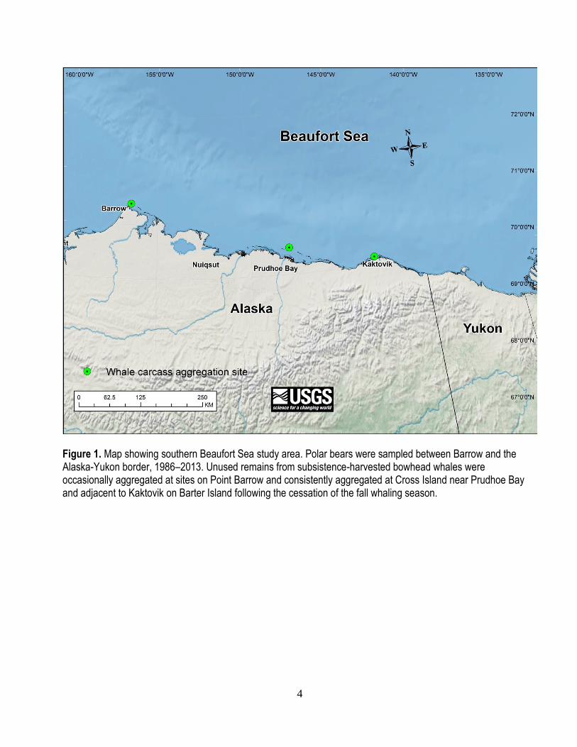
The study area was most of the Alaskan part of the SB, ranging from Demarcation Point (140°

W) at the U.S.−Canada border in the east to Point Barrow (156° W) in the west (fig. 1). The SB is

characterized by a narrow continental shelf with an abrupt shelf-break that gives way to some of the

deepest waters of the Arctic Ocean (Jakobsson and others, 2008). Historically, sea ice has remained over

or adjacent to the continental shelf year-round, even during the period of minimum sea ice extent in

September (Durner and others, 2009). However, over the last 15 years there has been a trend in the SB

of earlier sea ice break-up, reduced summer sea ice extent, and a lengthening of the open-water season

(Stroeve and others, 2014).

The SB coastal region is characterized by an industrial footprint associated with oil and gas

exploration and extraction activities. The Prudhoe Bay and Kuparuk oil fields are situated at the

approximate midpoint along the coast, and the National Petroleum Reserve of Alaska spans a significant

stretch of the western part of the coastal plain. As a result, polar bears that frequent this area can be

exposed to industrial activities (Amstrup and others, 2006). There are three communities on Alaska’s

North Slope (Barrow, Nuiqsut, and Kaktovik) that harvest bowhead whales in the fall. Unwanted

remains from the harvest are sporadically aggregated at Point Barrow (Barrow; west) and consistently

aggregated at Cross Island (Nuiqsut: remains aggregated on Cross Island near Prudhoe Bay; central) and

Barter Island (Kaktovik; east), and the three sites are nearly evenly spaced along the coast (fig. 1) where

they have served as focal attractors for polar bears (Schliebe and others, 2008).

4

Figure 1. Map showing southern Beaufort Sea study area. Polar bears were sampled between Barrow and the Alaska-Yukon border, 1986–2013. Unused remains from subsistence-harvested bowhead whales were occasionally aggregated at sites on Point Barrow and consistently aggregated at Cross Island near Prudhoe Bay and adjacent to Kaktovik on Barter Island following the cessation of the fall whaling season.

5

3.1. Data Collection

Polar bear research in the SB has been ongoing for more than 30 years, and we used both

historical and contemporary data sets to investigate whether land use has changed over time. Since the

mid-1980s, polar bears have been captured on the sea ice (up to 160 km from the coast) nearly every

spring. Additionally, some captures occurred on land in the fall of 2008, 2009, and 2010. All polar bears

were encountered opportunistically from a helicopter and immobilized with the drugs sernylan or

phencyclidine (prior to 1987) and tiletamine hydrochloride plus zolazepam hydrochloride (1987–2013;

Telazol®, Fort Dodge and Warner-Lambert Co.) using a projectile syringe fired from a dart gun. A

subset of adult females was fitted with Argos or global positioning system (GPS) platform transmitter

terminal (PTT) satellite radio collars (for example, Durner and others, 2009). Age was determined by

multiple methods. Cubs-of-the-year (COY) were always with their mothers and could be visually aged

without error (Ramsay and Stirling, 1988). Some bears had been captured and marked in previous years,

so their age was determined from their capture history. For new captures, we extracted a vestigial

premolar and determined age by analysis of cementum annuli (Calvert and Ramsay, 1998). Below, we

describe a sampling design that combined fine-scale satellite radio collar data collected from a relatively

small sample of individuals with coarser scale aerial survey data collected from a much larger sample of

individuals that allowed us to link individual behaviors to population-level responses to changing sea

ice phenology.

3.2. Demographic Composition, Relative Density, and Distribution

Polar bears are easy to detect when on land because of the contrast between the colors of bears

and the snow- and ice-free substrate (Stirling and others, 2004; Stapleton and others, 2014). When polar

bears of the SB come ashore, they mostly stay within a very narrow band of the coast or on barrier

islands (Schliebe and others, 2008), which differs in degree from traditional seasonal-ice subpopulations

(for example, Stapleton and others, 2014). Thus, surveys of the coastline and islands provide an index of

relative density and distribution for bears on shore (Stirling and others, 2004; Schliebe and others,

2008). From 2010 to 2013, we conducted transect-based aerial surveys twice (as much as 7 weeks apart;

range: August 18–October 3) each fall along the coast between Point Barrow and Demarcation Point to

estimate relative density and distribution on shore. In all years but 2013, the first survey was conducted

prior to the placement of bowhead whale remains at the bone piles, while the second survey was

conducted after the placement of remains. In 2013, both surveys were conducted after remains were

placed at bone piles. Transects were mostly 8-km-long and included segments oriented perpendicular to

the coast line connected by alternating inland or coastal segments (that is, a “sawtooth” pattern). A

subset of segments perpendicular to the coast line were 30-km-long to determine the extent to which

bears may be venturing inland. We flew Bell 206B and Aerostar 305A helicopters at an altitude of about

90 m and an airspeed of about 80 knots. Additionally, total counts were conducted over every barrier

island encountered, with the exception of Barter Island. The village of Kaktovik is located on Barter

Island and is adjacent to a bowhead whale carcass aggregation site, which provides opportunities for

commercial polar bear viewing. Commercial bear viewing became common in 2012 and we did not fly

over Barter Island in 2012 and 2013 over concerns that helicopter activity could disrupt viewing

opportunities. We did, however, obtain a ground-based total count of all bears present at the Barter

Island carcass site and local vicinity on the same day as our aerial surveys in 2012 and 2013 from the

U.S. Fish and Wildlife Service, which monitors polar bears in the immediate area. When we

encountered a bear during surveys, we estimated age, sex (for adults and subadults), group size, and

body condition, and collected a geo-referenced location. We estimated age of dependent young (cubs

and yearlings) and subadults (2–4 years old) based primarily on size. We estimated sex of adults and

6

subadults based on sexual dimorphism (males are larger), the absence or presence (males) of long guard

hairs on the forelimbs, and the absence or presence of a “swaying” gait for the hind limbs (males). We

also assigned each observation of sex and age class a confidence level of A (highly confident) or B

(moderately confident) and summarized the proportion observations for each confidence level to

characterize uncertainty of survey classifications. We combined counts from transects and barrier

islands to generate a total uncorrected minimum count for each of the two annual surveys. We expressed

relative density on shore as the total number of polar bears observed per 100 km of transect flown.

3.3. Phenology of Land Use and Length of Stay

We used location data collected from radiocollared adult females from 1986 to 2013 to

determine if bears used terrestrial habitat during summer/fall and, if so, to estimate mean dates of arrival

on shore and departure back to sea ice and duration of time spent on shore. Most locations prior to 2010

were derived from the Argos system, which has variable levels of accuracy, so we used standard

filtering methods (for example, Douglas and others, 2012) to remove spurious locations. We used the

continuous time correlated random walk (CRAWL) movement model (Johnson and others, 2008) to

estimate a regular time-series of daily locations (that is, expressed as latitude and longitude) from the

irregular observations of each animal. We used the R (R Development Core Team, 2013) package

‘crawl’ (Johnson and others, 2008) to implement the CRAWL model and predict daily polar bear

locations from July 1 to October 31. Because the CRAWL model does not provide meaningful results if

observed locations are too temporally dispersed, we excluded predicted locations that occurred between

observed points separated by more than 14 days, which generally precluded the detection of a distinct

movement signal (Hooten and others, 2014).

The CRAWL model allows predicted paths to take into account variable location quality,

sampling intervals, and changes in movement expected in different areas of the environment (for

example, land versus ice). Thus, for Argos locations, we defined location accuracy based on

designations for Telonics Argos collars (that is, L3: 150 m; L2: 350 m; L1: 1,000 m; L0: 1,500 m;

http://www.telonics.com/technotes/argosintro.php). Because location accuracies are not provided for

locations with LA or LB designations, we provided conservative location accuracies of LA: 5,000 m;

LB: 10,000 m. We assigned locations obtained from GPS collars an accuracy of 30 m (Frair and others,

2010). We then used a geographic information system to overlay the resulting daily movement paths on

land coverage shapefiles that included the coastline and barrier islands. We buffered the coastline and

islands by 5 km because the resolution of the coverage was, at times, not sufficient to detect small

barrier islands, which can receive disproportionate use by polar bears in summer (Gleason and Rode,

2009). We considered locations on land or within the buffer as occurring on land. For bears that came

ashore, we noted the ordinal date of arrival and departure, and calculated the total amount of time spent

on shore. We then generated estimates of arrival, departure, and length of stay as mentioned above.

3.4. Sea Ice Characteristics

Polar bears in the SB prefer sea ice habitat over the continental shelf because it provides greater

accessibility to prey than the deeper water of the polar basin (Durner and others, 2009). We

hypothesized that the density of bears on land and the phenology of land use was influenced by sea ice

characteristics, including the distance between the continental shelf break and the edge of the pack ice

and the concentration of ice over the shelf. We used daily sea ice data from the National Sea Ice Data

Center (Boulder, Colorado, USA) to develop concentration and distance metrics. Sea ice concentrations

were estimated from raster-format 25 × 25 km resolution passive microwave satellite imagery (Cavalieri

and others, 1996; updated continually). For July through October, we estimated a number of metrics

7

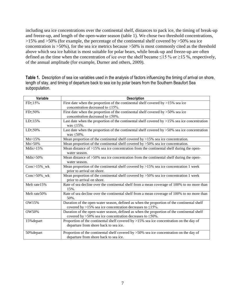
including sea ice concentrations over the continental shelf, distances to pack ice, the timing of break-up

and freeze-up, and length of the open-water season (table 1). We chose two threshold concentrations,

>15% and >50% (for example, the percentage of the continental shelf covered by >50% sea ice

concentration is >50%), for the sea ice metrics because >50% is most commonly cited as the threshold

above which sea ice habitat is most suitable for polar bears, while break-up and freeze-up are often

defined as the time when the concentration of ice over the shelf became ≤15 % or ≥15 %, respectively,

of the annual amplitude (for example, Durner and others, 2009).

Table 1. Description of sea ice variables used in the analysis of factors influencing the timing of arrival on shore, length of stay, and timing of departure back to sea ice by polar bears from the Southern Beaufort Sea subpopulation.

Variable Description

FD≤15% First date when the proportion of the continental shelf covered by >15% sea ice

concentration decreased to ≤15%.

FD≤50% First date when the proportion of the continental shelf covered by >50% sea ice

concentration decreased to ≤50%.

LD≤15% Last date when the proportion of the continental shelf covered by >15% sea ice concentration

was ≤15%.

LD≤50% Last date when the proportion of the continental shelf covered by >50% sea ice concentration

was ≤50%.

Mn>15% Mean proportion of the continental shelf covered by >15% sea ice concentration.

Mn>50% Mean proportion of the continental shelf covered by >50% sea ice concentration.

Mdis>15% Mean distance of >15% sea ice concentration from the continental shelf during the open-

water season.

Mdis>50% Mean distance of >50% sea ice concentration from the continental shelf during the open-

water season.

Conc>15%_wk Mean proportion of the continental shelf covered by >15% sea ice concentration 1 week

prior to arrival on shore.

Conc>50%_wk Mean proportion of the continental shelf covered by >50% sea ice concentration 1 week

prior to arrival on shore.

Melt rate15% Rate of sea decline over the continental shelf from a mean coverage of 100% to no more than

15%.

Melt rate50% Rate of sea decline over the continental shelf from a mean coverage of 100% to no more than

50%.

OW15% Duration of the open-water season, defined as when the proportion of the continental shelf

covered by >15% sea ice concentration decreases to ≤15%.

OW50% Duration of the open-water season, defined as when the proportion of the continental shelf

covered by >50% sea ice concentration decreases to ≤50%.

15%depart Proportion of the continental shelf covered by >15% sea ice concentration on the day of

departure from shore back to sea ice.

50%depart Proportion of the continental shelf covered by >50% sea ice concentration on the day of

departure from shore back to sea ice.

8

3.5. Characterizing Nutritional Condition

Adipose lipid content is an index of individual fat reserves (Cattet and others, 2002) and has

been shown to be an effective biochemical-based index of nutritional condition and health of polar bears

(McKinney and others, 2014). We collected subcutaneous adipose tissue samples with a 6 mm biopsy

punch from the rump region of anesthetized adult polar bears captured on sea ice each spring and on

land each fall between 2008 and 2009. Adipose tissue samples were kept frozen (-80 °C) prior to

analyses. Lipid was extracted from biopsy samples and individual lipid contents, reported as the ratio of

extracted lipid relative to initial wet weight of adipose tissue, were quantified as described in McKinney

and others (2014). We then compared lipid content between bears captured on land in fall to those

captured on the sea ice. The period of spring through the break-up of sea ice is when polar bears are

hyperphagic and feeding on vulnerable seal pups and molting adults (Stirling and Øritsland, 1995),

while the fall is generally the period of time when prey is least accessible due to reduced availability of

sea ice. Although it would be ideal to compare lipid content between bears on land to those on ice

during summer/fall, it was logistically infeasible to sample bears on the sea ice during that time.

Nevertheless, comparing nutritional condition between fall and spring periods may provide some insight

into the potential nutritional benefit or consequences of spending time on land.

3.6. Analyses

From the two annual surveys, we used data from the survey with the highest total count each

year to characterize the demographic composition and to estimate the relative density of bears on shore.

We summarized the proportion of bears observed by demographic class (excluding observations

classified as sex or age unknown) for each selected survey and for each spring capture season, 2010–13.

We then used Cochran-Mantel-Haenszel tests (Agresti, 1996) to examine the proportional representation

of demographic classes among years between fall survey and spring capture data sets. We compared the

composition between bears on shore in fall to those captured on the sea ice in spring to determine if the

former was representative of the population-at-large (that is, bears captured during spring).

We used the paired sets of annual aerial surveys to investigate whether the availability of

bowhead whale scavenge subsidies influenced polar bear distribution. We pooled data among years

from surveys conducted before and after the stocking of carcass aggregation sites (Point Barrow, Cross

Island, and Barter Island) with whale remains following the cessation of the fall whaling season. We

used Moran’s I statistic to test the hypothesis that polar bear sightings were spatially autocorrelated (that

is, individuals were not randomly distributed), and a geographic information system to determine the

Euclidean distance of each geo-referenced bear sighting to the closest carcass aggregation site. We then

used a Kolmogorov-Smirnov test to determine if the distribution of distances from carcass sites differed

between survey sessions―that is, whether the spatial distribution of bears differed prior to and after the

stocking of carcass sites.

We used a generalized additive mixed model (GAMM) with a binomial distribution to determine

whether the proportion of radiocollared polar bears using land ≥21 consecutive days changed over time.

We chose the threshold of ≥21 consecutive days because it has been used previously (Schliebe and

others, 2008) to describe long-term use of land and thus allows for comparison to the current study. The

≥21 consecutive days threshold also allows us to discriminate between short-term and long-term land

use, which is most consequential from an ecological standpoint. Based on the previously mentioned

CRAWL analysis, we coded land use or lack thereof by individuals as a binary response variable (that

is, 1 = individual used land, 0 = individual did not use land). Because some individuals were

radiocollared in multiple years, we used individual as a random factor; year was used as the fixed effect.

9

To determine the relationship between the phenology of onshore use by radiocollared bears and

sea ice dynamics, we examined the influence of sea ice conditions and characteristics on the timing of

arrival on shore, length of stay on shore, and timing of departure from shore back to the sea ice. For this

analysis, we included bears that came ashore for any period of time rather than ≥21 consecutive days.

We used the ordinal dates of arrival and departure, and total days spent on shore, averaged among

individual bears within years, as response variables. Predictor variables included measures of >15%

and >50% sea ice concentrations over the continental shelf (for example, Mn >15%, Mn >50%),

distance from the shelf of >15% and >50% sea ice (Mdis >15%, Mdis >50%), length of the open water

season defined as the periods of time when sea ice concentration remained ≤15 or ≤50% (OW 15%, OW

50%), and the time to reach ≤50% and ≤15% ice concentration thresholds (for example, rate 100 to

15%). We developed, a priori, sets of biologically plausible candidate models (for example, table 2) and

used Akaike’s information criterion values (Akaike, 1973) corrected for small sample bias (AICc) to aid

in determining top models. We considered models with ΔAICc values >2.0 to measurably differ in

information content (Burnham and Anderson, 2002). We used AICc to rank and compare models based

on ΔAICc and normalized Akaike weights wi, and used the sum of all wi for each variable to rank them

in order of importance. When faced with model uncertainty, we used model averaging to include that

uncertainty in the estimate of precision of the parameters of interest (Burnham and Anderson, 2002;

Arnold, 2010). We assessed multicollinearity of predictor variables using variance inflation factors

(VIF) and considered multicollinearity to be high when VIF >10 (Allison, 1999). We used normal

probability plots and coefficients of correlation to ensure that model variables were normally distributed

(Neter and others, 1996).

We used a general linear mixed model to compare lipid concentrations in adipose tissue samples

from bears captured on the sea ice in spring to those captured on land in fall, 2008–09. Because we

sampled some of the same individuals in both years, we included individual identity as a random factor.

Fixed effects included season (fall or spring), demographic class (adult female, adult male), and year.

We tested all two-way interactions of fixed factors and made a posteriori pairwise comparisons using

least squares means tests (Zar, 1999). We used the restricted maximum likelihood (REML) method for

model estimation and Satterthwaite’s F tests to gauge effects (McCullagh and Nelder, 1991). For all

statistical tests, significance was accepted at α ≤ 0.05.

10

Table 2. Example of hypotheses and variables used in candidate regression models tested to predict the timing of arrival on shore, length of stay on shore, and departure from shore by adult female polar bears, 1986–2013.

Model set Model no. Hypothesis Variables Timing of arrival 1 Arrival is influenced by the first date when the proportion

of the continental shelf covered by >15% sea ice

concentration decreased to ≤15%.

FD≤15%

2 Arrival is influenced by the proportion of the continental

shelf covered by >15% sea ice concentration.

Mn>15%

3 Arrival is influenced by the mean proportion of the

continental shelf covered by >15% sea ice concentration

1 week prior to arrival on shore.

Conc>15%_wk

4 Arrival is influenced by the rate of sea ice decline over the

continental shelf from a mean coverage of 100% to no

more than 50%.

Rate>50%

19 Null

Length of stay 1 Length of stay on shore is influenced by the duration of the

open-water season, defined as when the proportion of

the continental shelf covered by >15% sea ice

concentration decreases to ≤15%.

OW15%

2 Length of stay on shore is influenced by the proportion of

the continental shelf covered by >15% sea ice

concentration.

Mn>15% duration

3 Length of stay on shore is influenced by the mean distance

of >15% sea ice concentration from the continental shelf

during the open-water season.

Mdis>15% duration

4 Length of stay on shore is influenced by the mean distance

of >15% sea ice concentration from shore and the

duration of the 15% open-water season.

Mdis>15% duration,

OW15%

14 Null

Timing of

departure

1 Departure is influenced by the last date when the

proportion of the continental shelf covered by >15% sea

ice concentration was <15%.

LD≤15%

2 Departure is influenced by the mean distance of >15% sea

ice concentration from shore.

Mdis>15%

3 Arrival is influenced by the last date when the proportion

of the continental shelf covered by >15% sea ice

concentration was <15%, and the proportion of the shelf

covered by >15% sea ice concentration.

LD≤15%, >15%depart

4 Arrival is influenced by the last date when the proportion

of the continental shelf covered by >15% sea ice

concentration was <15%, and the proportion of the

continental shelf covered by >50% sea ice

concentration.

LD≤15%, >50%depart

15 Null

11

4.0. Results

During 2010–2013 fall aerial surveys, we flew a total of 9,820 km (mean = 1,226 km, SE = 134

km) on transect and searched an average of 31 barrier islands (table 3). The number of bears observed

differed within and between years, with the greatest number of bears detected during September

surveys. Distance surveyed was not related to the number of bears encountered per kilometer of transect

flown (Spearman’s r = -0.38, n = 8, P = 0.35), indicating that effort was likely sufficient to estimate

relative density.

Table 3. Aerial transect (coastal and perpendicular segments) survey and total count data for Barter and Cross islands, distance surveyed, and relative density of polar bears observed on shore, 2010–2013.

Survey date Survey count (total)

Barter Island count

Cross Island count Distance surveyed (kilometers)

Relative density

9/9/2010 29 12 9 1,626 0.018

10/3/2010 95 30 56 2,024 0.047

8/18/2011 74 18 19 1,192 0.062

9/23/2011 98 47 17 1,032 0.091

9/24/2012 140 43 69 832 0.168

9/29/2012 141 52 72 880 0.160

9/11/2013 93 50 21 1,040 0.089

9/22/2013 113 61 29 1,184 0.095

4.1. Demographic Composition and Relative Density

The proportions of sex/age classes observed on land in fall and on sea ice in spring were similar

across years (χ2 = 0.09, df = 1, P = 0.75), although minor differences existed (table 4). Adult males

made up the greatest proportion of individuals observed for both fall onshore surveys (0.30 ± 0.11) and

spring sea ice captures (0.32 ± 0.05). For fall surveys, the mean proportion of solitary adult females

(0.22 ± 0.16) was greater than the mean proportion of adult females with dependent young (0.15 ±

0.09). For spring captures, the mean proportion of adult females with dependent young (0.20 ± 0.01)

was greater than the mean proportion of solitary adult females (0.13 ± 0.04). Mean proportions of

subadults and dependent young were similar between fall surveys and spring captures (table 4). For fall

surveys, >88% of observations of sex and age class were assigned to confidence level A (highly

confident).

The relative density of bears observed on shore increased from the baseline (2000–2005)

average of 4 ± 2 bears/100 km (that is, 3.7% of the estimated population [1,526], as reported in Schliebe

and others, 2008) to an average of 9 ± 2 bears/100 km for the recent period (2010–2013; that is, 11.8%

of the estimated population [907] per Bromaghin and others, 2015). For the latter, the annual high

density estimates ranged from a minimum of 9 bears/100 km (10.4% of the estimated population) in

2011, to a maximum of about 17 bears/100 km (15.4% of the estimated population) in 2012. We

observed no polar bears beyond 8-km inland from the coast. During September 2000–2005, the distance

from the continental shelf to the leading edge of >15% sea ice concentration averaged 86 km (SE = 16

km), while the distance to >50% sea ice concentration averaged 171 km (SE = 17 km). For 2010–2013,

the distances from the shelf to >15% and >50% sea ice concentrations averaged 301 km (SE = 54 km)

and 458 km (SE = 66 km), respectively.

12

Table 4. Demography of polar bears observed on shore during fall aerial surveys and island total counts, and captured on sea ice during spring, 2010–2013.

Year

Adult females without

dependent young

Adult females with dependent

young

Adult males

Subadult females

Subadult males

Dependent young

Fall surveys

2010 0.18 0.22 0.18 0.03 0.02 0.38

2011 0.26 0.18 0.15 0.00 0.02 0.29

2012 0.03 0.17 0.42 0.04 0.04 0.05

2013 0.41 0.02 0.03 0.04 0.03 0.26

Spring captures

2010 0.13 0.18 0.30 0.02 0.02 0.29

2011 0.10 0.20 0.26 0.08 0.06 0.24

2012 0.11 0.21 0.37 0.08 0.06 0.16

2013 0.19 0.20 0.36 0.05 0.06 0.14

4.2. Distribution

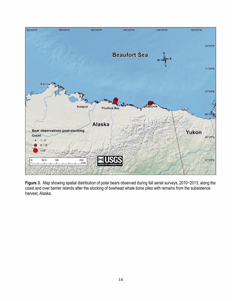
Moran’s I statistic indicated that polar bears were not randomly distributed when observed

during aerial surveys conducted prior to (z = 8.51, P <0.0001; fig. 2) and after (z = 15.08, P <0.0001;

fig. 3) the stocking of carcass aggregation sites. The percentage of polar bears located in close proximity

to bone piles was greater following the stocking of carcass sites (D = 0.14, P = 0.001). Prior to the

provisioning of bone piles, 64% of polar bear observations occurred within 16 km (that is, mean daily

distance traveled by SB polar bears; Amstrup and others, 2000) of an aggregation site. After scavenge

subsidies became available, 78% of all bears observed were within 16 km of an aggregation site. During

both sessions, we observed the greatest percentage of bears near Barter Island (40%), followed by Cross

Island (33%). Relatively few bears were observed in the vicinity of Point Barrow (<2%). The mean

distance from the coast for all bears observed on the mainland (rather than those observed on barrier

islands) was 0.38 km (range: 0.02–1.03 km) before scavenge subsidies became available and 1.73 km

after (range 0.05–9.05 km).

13

Figure 2. Map showing spatial distribution of polar bears observed during fall aerial surveys along the coast and over barrier islands prior to the stocking of bowhead whale bone piles with remains from the subsistence harvest, Alaska, 2010–13.

14

Figure 3. Map showing spatial distribution of polar bears observed during fall aerial surveys, 2010−2013, along the coast and over barrier islands after the stocking of bowhead whale bone piles with remains from the subsistence harvest, Alaska.

15

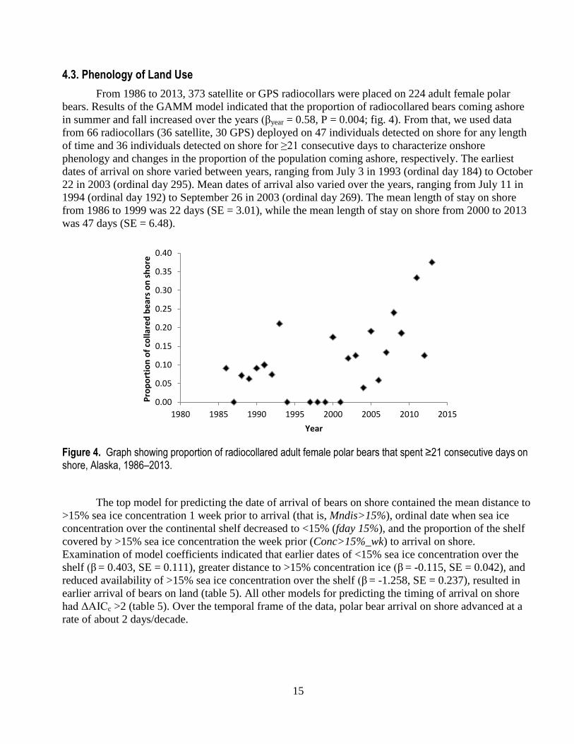
4.3. Phenology of Land Use

From 1986 to 2013, 373 satellite or GPS radiocollars were placed on 224 adult female polar

bears. Results of the GAMM model indicated that the proportion of radiocollared bears coming ashore

in summer and fall increased over the years (βyear = 0.58, P = 0.004; fig. 4). From that, we used data

from 66 radiocollars (36 satellite, 30 GPS) deployed on 47 individuals detected on shore for any length

of time and 36 individuals detected on shore for ≥21 consecutive days to characterize onshore

phenology and changes in the proportion of the population coming ashore, respectively. The earliest

dates of arrival on shore varied between years, ranging from July 3 in 1993 (ordinal day 184) to October

22 in 2003 (ordinal day 295). Mean dates of arrival also varied over the years, ranging from July 11 in

1994 (ordinal day 192) to September 26 in 2003 (ordinal day 269). The mean length of stay on shore

from 1986 to 1999 was 22 days (SE = 3.01), while the mean length of stay on shore from 2000 to 2013

was 47 days (SE = 6.48).

Figure 4. Graph showing proportion of radiocollared adult female polar bears that spent ≥21 consecutive days on shore, Alaska, 1986–2013.

The top model for predicting the date of arrival of bears on shore contained the mean distance to

>15% sea ice concentration 1 week prior to arrival (that is, Mndis>15%), ordinal date when sea ice

concentration over the continental shelf decreased to <15% (fday 15%), and the proportion of the shelf

covered by >15% sea ice concentration the week prior (Conc>15%_wk) to arrival on shore.

Examination of model coefficients indicated that earlier dates of <15% sea ice concentration over the

shelf (β = 0.403, SE = 0.111), greater distance to >15% concentration ice (β = -0.115, SE = 0.042), and

reduced availability of >15% sea ice concentration over the shelf (β = -1.258, SE = 0.237), resulted in

earlier arrival of bears on land (table 5). All other models for predicting the timing of arrival on shore

had ΔAICc >2 (table 5). Over the temporal frame of the data, polar bear arrival on shore advanced at a

rate of about 2 days/decade.

0.00

0.05

0.10

0.15

0.20

0.25

0.30

0.35

0.40

1980 1985 1990 1995 2000 2005 2010 2015

Pro

po

rtio

n o

f co

llare

d b

ear

s o

n s

ho

re

Year

16

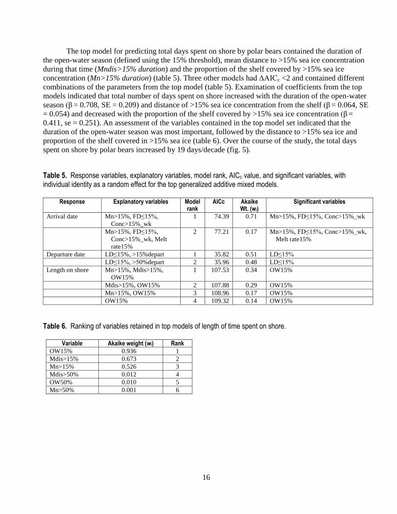
The top model for predicting total days spent on shore by polar bears contained the duration of

the open-water season (defined using the 15% threshold), mean distance to >15% sea ice concentration

during that time (Mndis>15% duration) and the proportion of the shelf covered by >15% sea ice

concentration (Mn>15% duration) (table 5). Three other models had ΔAICc <2 and contained different

combinations of the parameters from the top model (table 5). Examination of coefficients from the top

models indicated that total number of days spent on shore increased with the duration of the open-water

season (β = 0.708, SE = 0.209) and distance of >15% sea ice concentration from the shelf (β = 0.064, SE

= 0.054) and decreased with the proportion of the shelf covered by >15% sea ice concentration (β =

0.411, se = 0.251). An assessment of the variables contained in the top model set indicated that the

duration of the open-water season was most important, followed by the distance to >15% sea ice and

proportion of the shelf covered in >15% sea ice (table 6). Over the course of the study, the total days

spent on shore by polar bears increased by 19 days/decade (fig. 5).

Table 5. Response variables, explanatory variables, model rank, AICc value, and significant variables, with individual identity as a random effect for the top generalized additive mixed models.

Response Explanatory variables Model rank

AICc Akaike Wt. (wi)

Significant variables

Arrival date Mn>15%, FD≤15%,

Conc>15%_wk

1 74.39 0.71 Mn>15%, FD≤15%, Conc>15%_wk

Mn>15%, FD≤15%,

Conc>15%_wk, Melt

rate15%

2 77.21 0.17 Mn>15%, FD≤15%, Conc>15%_wk,

Melt rate15%

Departure date LD≤15%, >15%depart 1 35.82 0.51 LD≤15%

LD≤15%, >50%depart 2 35.96 0.48 LD≤15%

Length on shore Mn>15%, Mdis>15%,

OW15%

1 107.53 0.34 OW15%

Mdis>15%, OW15% 2 107.88 0.29 OW15%

Mn>15%, OW15% 3 108.96 0.17 OW15%

OW15% 4 109.32 0.14 OW15%

Table 6. Ranking of variables retained in top models of length of time spent on shore.

Variable Akaike weight (wi) Rank

OW15% 0.936 1

Mdis>15% 0.673 2

Mn>15% 0.526 3

Mdis>50% 0.012 4

OW50% 0.010 5

Mn>50% 0.001 6

17

Figure 5. Graph showing mean (and standard error) length of stay on shore relative to the length of the open-water season, defined as the time when the proportion of the continental shelf covered by >15% sea ice concentration decreases to ≤15%.

The top model for predicting the date of departure of bears from shore back to the sea ice

contained the ordinal date when sea ice concentration over the shelf first increased to >15% (lday 15%;

β = 0.127, SE = 0.048) and the proportion of the shelf covered by >15% sea ice concentration the week

prior to departure (shelf>15% depart; β = -0.117, SE = 0.191) (table 5). The second ranked model

contained lday 15% (β = 0.131, SE = 0.051) and the proportion of the shelf covered by >50% sea ice

concentration the week prior to departure (shelf>15% depart; β = -0.097, SE = 0.218). Evidentiary

weights of the two top models were similar, and assessment of the variable set indicated that the ordinal

date variable was most important (table 7). Over the duration of the study, the date of departure of bears

from shore became later by 10 days/decade.

Table 7. Ranking of variables retained in top models of date of departure from shore back to the sea ice.

Variable Akaike weight (wi) Rank

LD<15% 0.999 1

>15%depart 0.517 2

>50%depart 0.483 3

Mdis>50% <0.001 4

LD<50% <0.001 5

Mdis<15% <0.001 6

18

4.4. Characterizing Nutritional Condition

Lipid content of adipose tissue samples differed by season of collection (GLMM: F1,45 = 35.31,

P < 0.001) but not by demographic class (F1,45 = 0.27, P = 0.60) or year (F1,45 = 1.59, P = 0.21). Mean

lipid contents were higher for bears sampled on land in the fall (adult females: 0.56 ± 0.11; adult males:

0.51 ± 0.15) than for those sampled during the hyperphagic period in the spring (adult females: 0.36 ±

0.19; adult males: 0.39 ± 0.15). Pairwise comparisons indicated that mean lipid contents were

significantly higher in fall for adult females and adult males. No two-way interactions were significant.

Discussion

Historical (that is, pre-2000) use of terrestrial habitat during the open-water season by SB polar

bears was relatively rare and limited to short durations (for example, Amstrup and others, 2000). The

patterns of use from the early 2000s (that is, Schliebe and others, 2008) and those that we observed

during our study suggest this behavior has become more prevalent, although most of the SB population

still remains on sea ice during summer. We detected an increase in the relative density of polar bears on

shore, an increase in the percentage of radiocollared bears coming ashore, later dates of departure, and

lengthening land tenure over time. Furthermore, increased use of terrestrial habitat was related to

declines in sea ice extent and changing sea ice phenology. Since the late 1990s, the duration of the open-

water season in the SB increased by an average of 32 and 36 days based on >50% and >15% sea ice

concentrations over the continental shelf, respectively, while the amount of time spent on land increased

by about 3 weeks.

The relatively infrequent historical use of onshore habitat by SB polar bears was likely due to the

persistent availability of sea ice over the continental shelf, even during the period of minimum sea ice

extent in September, although we cannot rule out the availability of scavenge subsidies as a contributing

causative factor. Since the late 1990s, the duration of the open-water season in the SB increased by 66%

or 82% (depending on sea ice concentration threshold), while the mean distance from shore to pack ice

in September increased by as much as 120%. The most dramatic changes have occurred recently with

the seven lowest September Arctic-wide sea ice extents observed over the last 7 years of our time series

(Stroeve and others, 2014). From 2006 to 2013, the distance from shore to September pack ice increased

by 66%, which placed the leading edge of the ice an average of 458 km from the continental shelf. Polar

bears prefer to forage from sea ice over shallow, biologically productive continental shelf waters

(Durner and others, 2009). The extended seasonal loss of sea ice over the shelf equates to a functional

loss of preferred foraging habitat. Evidence suggests that displaced polar bears are increasingly coming

ashore in response.

19

Previous work in the SB (Schliebe and others, 2008) and elsewhere (for example, WHB; Stirling

and others, 1999) has found that the timing of arrival and relative density of bears on shore were

correlated with ≥50% sea ice concentrations. More recently, Cherry and others (2013) evaluated

multiple sea ice concentration thresholds in WHB to determine that dates of arrival were best correlated

with the timing of 30% sea ice concentration, while departure occurred after ice concentrations reached

>10%. Our findings that the availability of sea ice concentrations >15% are best correlated with the

timing of arrival, length of stay, and timing of departure of SB bears, are qualitatively similar to the

findings of Cherry and others (2013). It appears that in both subpopulations, polar bears delay the

transition from ice to shore as long as possible―that is, until sea ice declines to less than a

concentration where its use as a reliable hunting platform is untenable. This information is important

quantitative evidence of the relationship between sea ice phenology and use of terrestrial habitat by

polar bears. Monitoring the timing and rate of seasonal ice disappearance may be an effective,

logistically tractable, way for managers and industry to prepare for the annual arrival of bears on shore.

Aerial surveys indicated that the relative density of bears on shore during summer has increased

since the early to mid-2000s (Schliebe and others, 2008). Our survey methodology differed from

Schliebe and others (2008) in that we included 8-km and 30-km segments that ran perpendicular to the

coast rather than only segments parallel to the coast. If those perpendicular segments are removed, the

coastal densities listed in table 3 would be even higher. From 2005 to 2008, there was a notable decline

in the survival and abundance of SB polar bears, followed by 2 years (2009–2010) of apparent stability

(Bromaghin and others, 2015). The declines and subsequent stability of survival and abundance

occurred while use of terrestrial habitat was increasing. Although there is no causal link between the

patterns in polar bear vital rates and increased use of terrestrial habitat, there is precedence for

behavioral shifts ameliorating some of the adverse effects of rapid environmental change. For example,

Charmentier and others (2008) found that individual adjustment of behavior allowed a population of

great tits (Parus major) to closely track changes in prey phenology and maintain the temporal match

between clutch hatch date and peak availability of prey. This suggests that behavioral adjustments that

closely track key phenological shifts may lessen some impacts of rapid environmental change, at least in

the short term. The decision to exploit terrestrial habitat, rather than remain with the retreating pack ice,

is clearly a behavioral response to the loss of sea ice habitat over the continental shelf. Whether bears

benefit from that behavioral response will likely hinge on the trade-off between the availability of food

resources and increased exposure to human-related activities.

Distribution data obtained from aerial surveys suggests that bowhead whale bone piles in the SB

are focal attractors for bears on shore. Rogers and others (2015) found evidence of a shift in foraging

behavior by some SB polar bears marked by fidelity to the nearshore region of sea ice during spring and

consumption of bowhead whale tissue during summer and fall. Most bowhead whale tissue likely is

consumed by bears visiting bone piles that have been stocked with remains following fall whaling

(Herreman and Peacock, 2013), although scavenging on beach-cast whales also occurs. Regardless of

whether bears scavenge beach-cast or human-provisioned remains, they appear to be in better nutritional

condition than bears sampled on the ice in the spring, although it is important to note that polar bears are

known to reach minimum body mass in late March (Stirling, 2002), which coincides with the start of

our spring sampling period. Furthermore, the timing of collection of adipose tissue samples from bears

in the fall likely was not ideal for capturing the effect that feeding on bowhead whale remains might

have on body condition. Nevertheless, the availability of marine mammal food resources to bears on

shore is an important distinction between the SB and the five seasonal ice subpopulations. For the latter,

entire subpopulations come ashore when the annual ice melts completely each summer and bears enter a

hypophagic state until the ice reforms in the fall (Amstrup and others, 2008). In WHB, the open-water

20

season lasts upwards of 4 months (for example, Stirling and Parkinson, 2006), and model-based

estimates suggest that an increase beyond 5 months could trigger declines in reproductive potential and

survival (for example, Molnar and others, 2010 and 2014; Robbins and others, 2012). Currently in the

SB, bears are spending upwards of 2.5 months on shore and have access to food for the latter portion of

that period. If the trend of increasing use of terrestrial habitat and lengthening open-water season

increase in the SB, then the relative benefits of scavenging at bone piles should diminish over time.

Although changes in sea ice availability and phenology may be mediating the density and length

of time bears spend on shore, the predictable availability of scavenge subsidies at bone piles are likely

facilitating the extended use of onshore habitats. Increased use of terrestrial habitat and exploitation of

human-provisioned resources by polar bears has attendant risks, including a greater potential for human-

polar bear interactions. Wildlife-human conflict can have wide-ranging effects, including adversely

impacting wildlife populations, causing economic losses to stakeholders and endangering public safety

(Thirgood and others, 2005). The northern coast of Alaska includes several villages and an industrial

footprint associated with oil exploration and extraction activities, all of which are in relatively close

proximity to bowhead whale bone piles (particularly at Barter and Cross Islands) where most bears were

detected during aerial surveys. Polar bears that are highly motivated to obtain food appear more willing

to risk interacting with humans (for example, Towns and others, 2009), and the increased frequency of

bears on land, coupled with an increase in human activity enabled by retreating sea ice, is expected to

result in a greater risk of human-polar bear interaction and conflict.

The juxtaposition of aggregated bears and humans at Barter and Cross Islands exemplifies the

potential breadth of risks that SB bears may be exposed to if their reliance on terrestrial habitat

increases. In the case of Barter Island, the bone pile is adjacent to the community of Kaktovik

(population 293; 2010 U.S. Census), where commercial bear viewing and food attractants raise the risk

of contest-based (that is, a “scramble” to partition finite resources; Isbell, 1991) human-polar bear

interactions and increased potential for defense of life kills. Additionally, the area around Cross Island is

dominated by human activities related to resource extraction, which also exposes bears to risks,

including exposure to contaminants/industrial solvents (for example, Amstrup and others, 1989) and oil

spills (Amstrup and others, 2006). Mitigating the risks to polar bears and humans is further complicated

by the fact that interaction and conflict are often clustered in space and time (for example, Baruch-

Mordo and others, 2008) because of the availability and distribution of focal attractors. Given that the

extent of summer sea ice is projected to decline through the 21st century (Overland and Wang, 2013),

terrestrial habitat and human-provisioned resources are likely to become increasingly important for SB

polar bears. Although some efforts to minimize human-polar bear interactions are already underway,

increased efforts to proactively manage food attractants and exposure to pollutants will be needed to

reduce the risk of conflict to communities and industry.

Our study suggests that SB polar bears have become more reliant on terrestrial habitat and

human-provisioned marine mammal resources. The ecological consequences of this behavioral shift are

largely unknown, but are likely to be manifested as altered community interactions in both marine and

terrestrial ecosystems. Polar bears are an apex predator in the marine ecosystem, and seasonal shifts in

diet to terrestrial resources and the resulting release of marine prey from predation may induce changes

in primary prey behavior and alter the distribution of scavengers that rely on polar bear kills (for

example, Roth, 2003). Likewise, increased use of terrestrial habitat may lead to novel interactions with

land-based prey and putative competitor species. For example, Prop and others (2015) found that the

increased occurrence of bears on land at Svalbard and east Greenland led to high rates of nest predation

on some colonially nesting bird species, particularly when bears arrived well in advance of the hatch.

Lastly, increasing use of terrestrial habitats by polar bears may increase the likelihood of competitive

21

interactions with sympatric brown bears (Ursus arctos; Miller and others, 2015). Changing distributions

and behaviors of polar bears and brown bears in the Arctic in response to climate change have the

potential to increase their interactions including increase competition for terrestrial space and food

resources.

Since the mid-2000s, the estimated proportion of the SB subpopulation coming ashore (for

example, Schliebe and others, 2008) has increased substantially, and the behavior should no longer be

considered trivial, even though most of the population still remains with the sea ice during the open-

water season. Indeed, there is reason to hypothesize that use of terrestrial habitat may be adaptive, at

least for the short-term. When summer sea ice persists in the SB, it is now relegated to the deep water of

the polar basin, which is less biologically productive than the continental shelf region. As a result, polar

bears that remain with the ice may have fewer opportunities to encounter ringed and bearded

(Erignathus barbatus) seals, which may explain reports of decreased kill rates, increased frequency of

fasting (Cherry and others, 2009; Pilfold and others, 2015), and declining body condition (Rode and

others, 2010). By contrast, polar bears that come ashore and scavenge at bone piles may be able to

maximize energy intake while minimizing energy expended, thereby reducing the likelihood of fasting

and staving off declines in body condition.

Polar bears have evolved preferences for sea ice habitat and marine mammal prey. In the SB,

those preferences are informing two seemingly disparate strategies for coping with the loss of summer

sea ice habitat: displace to shore and scavenge on predictably available marine mammal prey or remain

with the sea ice as it retracts over the polar basin and risk nutritional restriction (Rogers and others,

2015). It is unknown whether one or both strategies may be maladaptive over time. Human-induced

rapid environmental change is having profound effects on the quality and quantity of Arctic sea ice (for

example, Lindsay and Zhang, 2005; Maslanik and others, 2007), which is likely to make it difficult for

polar bears and other ice-adapted species to reliably select suitable habitats for maintaining fitness (Hale

and others, 2015). Behavioral plasticity is the initial response to dramatic environmental perturbations,

followed by transmission of innovative behaviors within and across generations, eventually leading to

evolution of the behavioral response over time (Tuomainen and Candolin, 2011). However, behavioral

plasticity may be an effective response by polar bears only if the rate of environmental change does not

outpace transmission of behavioral innovations.

Acknowledgments

We thank Dave Yokel (Bureau of Land Management) and Brian Glaspell (Arctic National

Wildlife Refuge) for continued support of our research program. George Durner, Kristin Simac,

Anthony Pagano, Tyrone Donnelly, Geoff York, and Steve Amstrup of the U.S. Geological Survey were

instrumental in collecting long-term data. Michelle St. Martin and Charles Hamilton of the U.S. Fish

and Wildlife Service assisted with the collection of count data on Barter Island. We thank Dave Douglas

and Jeff Bromaghin of the U.S. Geological Survey for providing sea ice data and advice on statistical

analyses, respectively. Lastly, we thank Doc Gohmert (Prism Helicopters), Howard Reed (Maritime

Aviation), and Joe Fieldman (Soloy Helicopters) for their skillful and safe piloting of helicopters.

Additional funding was provided by the Bureau of Land Management and the U.S. Geological

Survey’s Changing Arctic Ecosystems, Wildlife Program of the Ecosystems and Climate and Land Use

Change mission areas. We thank Karen Oakley, John Pearce, William Beatty of the U.S. Geological

Survey, and Stewart Breck of the National Wildlife Research Center for reviewing earlier drafts of this

report.

22

References Cited

Aars, J., Lunn, N.J., and Derocher, A.E., eds., 2006, Polar bears—Proceedings of the 14th Working

Meeting of the IUCN/SSC Polar Bear Specialist Group, June 20−24, 2005, Seattle, Washington,

USA: Gland, Switzerland and Cambridge, United Kingdom, IUCN, 189 p.

Agresti, A., 1996, An introduction to categorical analysis: New York, John Wiley and Sons, 290 p.

Akaike, H., 1973, Maximum likelihood identification of Gaussian autoregressive moving average

models: Biometrika, v. 60, p. 255−265.

Allison, P.D., 1999, Multiple regression—A primer: Newbury Park, California, Pine Forge Press, 202 p.

Amstrup, S.C., Durner, G.M., McDonald, T.L., and Johnson, W.R., 2006, Estimating potential effects of

hypothetical oil spills on polar bears: U.S. Geological Survey Open-File Report 2006-1337.

Amstrup, S.C., Durner, G.M., Stirling, I., Lunn, N.J., and Messier, F., 2000, Movements and

distribution of polar bears in the Beaufort Sea: Canadian Journal of Zoology, v. 78, p. 948–966.

Amstrup, S.C., Gardner, C., Meyers, K.C., and Oehme, F.W., 1989, Ethylene glycol (antifreeze)

poisoning of a free-ranging polar bear: Veterinary and Human Toxicology, v. 3, p. 317–319.

Amstrup, S.C., Marcot, B.G., and Douglas, D.C., 2008, A Bayesian network modeling approach to

forecasting the 21st century worldwide status of polar bears, in DeWeaver, E.T., Bitz, C.M., and

Tremblay, L.- B., eds., Arctic sea ice decline—Observations, projections, mechanisms, and

implications: Washington, D.C., American Geophysical Union Geophysical Monograph No. 180, p.

213–268.

Arnold, T.W., 2010, Uninformative parameters and model selection using Akaike's Information

Criterion: The Journal of Wildlife Management, v. 74, p. 1175−1178.

Atwood, T.C., Marcot, B., Douglas, D., Amstrup, S., Rode, K., Durner, G., and Bromaghin, J., 2015,

Evaluating and ranking threats to the long-term persistence of polar bears: U.S. Geological Survey

Open-File Report 2014-1254.

Baruch-Mordo, S., Breck, S.W., Wilson, K.R., and Theobald, D.M., 2008, Spatiotemporal distribution

of black bear-human conflicts in Colorado, USA: Journal of Wildlife Management, v. 72, p.

1,853−1,862.

Bromaghin, J.F., McDonald, T.L., Stirling, I., Derocher, A.E., Richardson, E.S., Regehr, E.V., Douglas,

D.C., Durner, G.M., Atwood, T.C., and Amstrup, S.C., 2015, Polar bear population dynamics in the

southern Beaufort Sea during a period of sea ice decline: Ecological Applications, v. 25, p. 634−651.

Burnham, K.P., and Anderson, D.R., 2002, Model selection and multimodel inference—A practical

information-theoretic approach (2nd ed.): New York, Springer, New York, 488 p.

Calvert, W., Branigan, M., Cattet, M., Doidge, W., Elliott, C., Lunn, N.J., Messier, F., Obbard, M.,

Otto, R., Ramsay, M., Stirling, I., Taylor, M., and Vandal, D., 2002, Polar bear management in

Canada 1997–2000, in Lunn, N.J., Schliebe, S., and Born, E.W., eds., Polar bears—Proceedings of the

13th Working Meeting of the IUCN/SSC Polar Bear Specialist Group, June 23–28, 2001, Nuuk,

Greenland: Gland, Switzerland and Cambridge, United Kingdom, IUCN, p. 41–52.

Calvert, W., and Ramsay, M.A., 1998, Evaluation of age determination of polar bears by counts of

cementum growth layer groups: Ursus, v. 10, p. 449−453.

Cattet, M.R., Caulkett, N.A., Obbard, M.E., and Stenhouse, G.B., 2002, A body-condition index for

ursids: Canadian Journal of Zoology, v. 80, p. 1156−1161.

23

Cavalieri, D.J., Parkinson, C.L., Gloersen, P., and Zwally, H., 1996 (updated continually), Sea ice

concentrations from Nimbus-7 SMMR and DMSP SSM/I-SSMIS passive microwave data: Boulder,

Colorado, NASA National Snow and Ice Data Center Distributed Active Archive Center.

Charmantier, A., McCleery, R.H., Cole, L.R., Perrins, C., Kruuk, L.E.B., and Sheldon, B.C., 2008,

Adaptive phenotypic plasticity in response to climate change in a wild bird population: Science,

v. 320, p. 800−803.

Cherry, S.G., Derocher, A.E., Stirling, I., and Richardson, E.S., 2009, Fasting physiology of polar bears

in relation to environmental change and breeding behavior in the Beaufort Sea: Polar Biology, v. 32,

p. 383−391.

Cherry, S.G., Derocher, A.E., Thiemann, G.W., and Lunn, N.J., 2013, Migration phenology and

seasonal fidelity of an Arctic marine predator in relation to sea ice dynamics: Journal of Animal

Ecology, v. 82, p. 912–921.

Douglas, D.C., Weinzierl, R.C., Davidson, S., Kays, R., Wikelski, M., and Bohrer, G., 2012,

Moderating Argos location errors in animal tracking data: Methods in Ecology and Evolution, v. 3,

p. 999–1,007.

Durner, G.M., Douglas, D.C., Nielson, R.M., Amstrup, S.C., McDonald, T.L., Stirling, I., Mauritzen,

M., Born, E.W., Wiig, O., DeWeaver, E., Serreze, M.C., Belikov, S., Holland, M., Maslanik, J.A.,

Aars, J., Bailey, D.A., and Derocher, A.E., 2009, Predicting 21st-Century polar bear habitat

distribution from global climate models: Ecological Monographs, v. 79, p. 25–58.

Frair, J.L., Fieberg, J., Hebblewhite, M., Cagnacci, F., DeCesare, N.J., and Pedrotti, L., 2010, Resolving

issues of imprecise and habitat-biased locations in ecological analyses using GPS telemetry data:

Philosophical Transactions of the Royal Society B, v. 365, p. 2,187–2,200.

Gautier, D.L., Bird, K.J., Charpentier, R.R., Grantz, A., Houseknecht, D.W., Klett, T.R., Moore, T.E.,

Pitman, J.K., Schenk, C.J., Schuenemeyer, J.H., Sorenson, K., Tennyson, M.E., Valin, Z.C., and

Wandrey, C.J., 2009, Assessment of undiscovered oil and gas in the arctic: Science, v. 324, p. 1,175–

1,179.

Gleason, J.S., and Rode, K.D., 2009, Polar bear distribution and habitat association reflect long-term

changes in fall sea ice conditions in the Alaskan Beaufort Sea: Arctic, v. 62, p. 405−417.

Herreman, J., and Peacock, E., 2013, Polar bear use of a persistent food subsidy—Insights from non-

invasive genetic sampling in Alaska: Ursus, v. 24, p. 148−163.

Hale, R., Treml, E.A., and Swearer, S.E., 2015, Evaluating the metapopulation consequences of

ecological traps—Proceedings of the Royal Society of London B: Biological Sciences, v. 282,

doi:10.1098/rspb.2014.2930.

Hobson, K.A., and Stirling, I., 1997, Low variation in blood δ13C among Hudson Bay polar bears—

Implications for metabolism and tracing terrestrial foraging: Marine Mammal Science, v. 13,

p. 359−367.

Hobson, K.A., Stirling, I., and Andriashek, D.S., 2009, Isotopic homogeneity of breath CO2 from

fasting and berry-eating polar bears—Implications for tracing reliance on terrestrial foods in a

changing Arctic: Canadian Journal of Zoology, v. 87, p. 50−55.

Hooten, M.B., Hanks, E.M., Johnson, D.S., and Alldredge, M.W., 2014, Temporal variation and scale in

movement-based resource selection functions: Statistical Methodology, v. 17, p. 82−98.

24

Hunter, C.M., Caswell, H., Runge, M.C., Regehr, E.V., Amstrup, S.C., and Stirling, I., 2010, Climate

change threatens polar bear populations—A stochastic demographic analysis: Ecology, v. 91,

p. 2,883−2,897.

Isbell, L.A., 1991, Contest and scramble competition—Patterns of female aggression and ranging

behavior among primates: Behavioral Ecology, v. 2, p. 143–155.

Jakobsson, M., Macnab, R., Mayer, L., Anderson, R., Edwards, M., Hatzky, J., Schenke, H.W., and

Johnson, P., 2008, An improved bathymetric portrayal of the Arctic Ocean—Implications for ocean

modeling and geological, geophysical and oceanographic analyses: Geophysical Research Letters,

v. 35, L07602, doi:10.1029/2008GL033520.

Johnson, D.S., London, J.M., Lea, M.-A., and Durban, J.W., 2008, Continuous-time correlated random

walk model for animal telemetry data: Ecology, v. 89, p. 1028−1215.

Lindsay, R.W., and Zhang, J., 2005, The thinning of Arctic sea ice, 1988-2003—Have we passed a

tipping point?: Journal of Climate, v. 18, p. 4879−4894.

Maslanik, J.A., Fowler, C., Stroeve, J., Drobot, S., Zwally, J., Yi, D., and Emery, W., 2007, A younger,

thinner Arctic ice cover—Increased potential for rapid, extensive sea-ice loss: Geophysical Research

Letters, v. 34, L24501, doi:10.1029/2007GL032043.

McCullagh, P., and Nelder, J.A., 1991, Generalized linear models: London, Chapman and Hall.

McKinney, M.A., Atwood, T., Dietz, R., Sonne, C., Iverson, S.J., and Peacock, E., 2014, Validation of

adipose lipid content as a body condition index for polar bears: Ecology and Evolution, v. 4,

p. 516−527.

Miller, S., Wilder, J., and Wilson, R.R., 2015, Polar bear-grizzly bear interactions during the autumn

open-water period in Alaska: Journal of Mammalogy, http://dx.doi.org/10.1093/jmammal/gyv140.

Molnár, P.K., Derocher, A.E., Thiemann, G.W., and Lewis, M.A., 2010, Predicting survival,

reproduction and abundance of polar bears under climate change: Biological Conservation, v. 143, p.

1,612–1,622.

Molnár, P.K., Derocher, A.E., Thiemann, G.W., and Lewis, M.A., 2014, Corrigendum to “Predicting

survival, reproduction and abundance of polar bears under climate change” [Biol. Conserv. 143

(2010) 1612−1622]: Biological Conservation, v. 177, p. 230−231.

Neter, J., Kutner, M.H., Nachtsheim, C.J., and Wasserman, W., 1996, Applied linear statistical models:

Boston, McGraw-Hill, 1,408 p.

Obbard, M.E., Stapleton, S., Middel, K.R., Thibault, I., Brodeur, V., and Jutras, C., 2015, Estimating the

abundance of the Southern Hudson Bay polar bear subpopulation with aerial surveys: Polar Biology,

doi:10.1007/s00300-015-1737-5.

Obbard, M.E., Thiemann, G.W., Peacock, E., and DeBruyn, T.D., eds., 2010, Polar bears—Proceedings

of the 15th Working Meeting of the IUCN/SSC Polar Bear Specialist Group, June 29–July 3, 2009,

Copenhagen, Denmark: Gland, Switzerland and Cambridge, United Kingdom, IUCN, 235 p.

Overland, J.E., and Wang, M., 2013, When will the summer Arctic be nearly ice free?: Geophysical

Research Letters, v. 40, p. 2,097−2,101.

Peacock, E., Taylor, M.K., Laake, J., and Stirling, I. 2013, Population ecology of polar bears in Davis

Strait, Canada and Greenland: The Journal of Wildlife Management, v. 77, p. 463–476.

Pilfold, N.W., Derocher, A.E., Stirling, I., and Richardson, E., 2015, Multi-temporal factors influence

predation for polar bears in a changing climate: Oikos, doi: 10.1111/oik.02000.

25

Prop, J., Aars, J., Bårdsen, B.J., Hanssen, S.A., Bech, C., Bourgeon, S., de Fouw, J., Gabrielsen, G.W.,

Land, J., Noreen, E., Oudman, T., Sittler, B., Stempniewicz, L., Tombre, I., Wolters, E., and Moe, B.,

2015, Climate change and the increasing impact of polar bears on bird populations: Frontiers in

Ecology and Evolution, v. 3, no. 33., doi: 10.3389/fevo.2015.00033.

R Development Core Team, 2013, R—A language and environment for statistical computing: Vienna,

Austria, R Foundation for Statistical Computing.

Ramsay, M.A., and Stirling, I., 1988, Reproductive biology and ecology of female polar bears (Ursus

maritimus): Journal of Zoology, v. 214, p. 601−634.

Regehr, E.V., Amstrup, S.C., and Stirling, I., 2006, Polar bear population status in the southern Beaufort

Sea: U.S. Geological Survey Open-File Report 2006-1337.

Regehr, E.V., Hunter, C.M., Caswell, H., Amstrup, S.C., and Stirling, I., 2010, Survival and breeding of

polar bears in the southern Beaufort Sea in relation to sea ice: Journal of Animal Ecology, v. 79,

p. 117−127.

Robbins, C.T., Lopez-Alfaro, C., Rode, K.D., Tøien, Ø., and Nelson, L.O., 2012, Hibernation and

seasonal fasting in bears—The energetic costs and consequences for polar bears: Journal of

Mammalogy, v. 93, p. 1,493−1,503.

Rode, K.D., Amstrup, S.C., and Regehr, E.V., 2010, Reduced body size and cub recruitment in polar

bears associated with sea ice decline: Ecological Applications, v. 20, p. 768−782.

Rode, K.D., Regehr, E.V., Douglas, D.C., Durner, G., Derocher, A.E., Thiemann, G.W., and Budge,

S.M., 2014, Variation in the response of an Arctic top predator experiencing habitat loss—Feeding

and reproductive ecology of two polar bear populations: Global Change Biology, v. 20, p. 76–88.

Rogers, M.C., Peacock, E., Simac, K., O’Dell, M.B., and Welker, J.M., 2015, Diet of female polar bears

in the southern Beaufort Sea of Alaska: evidence for an emerging alternative foraging strategy in

response to environmental change: Polar Biology, v. 38, p. 1–13.

Roth, J.D., 2003, Variability in marine resources affects arctic fox population dynamics: Journal of

Animal Ecology, v. 72, p. 668−676.

Schliebe, S., Rode, K.D., Gleason, J.S., Wilder, J., Proffitt, K., Evans, T.J., and Miller, S., 2008, Effects

of sea ice extent and food availability on spatial and temporal distribution of polar bears during the

fall open-water period in the Southern Beaufort Sea: Polar Biology, v. 31, p. 999−1,010.

Smith, L.C., and Stephenson, S.R., 2013, New Trans-Arctic shipping routes navigable by midcentury:

Proceedings of the National Academy of Sciences, v. 110, p. 4,871–4,872.

Stapleton, S., Atkinson, S., Hedman, D., and Garshelis, D., 2014, Revisiting Western Hudson Bay:

Using aerial surveys to update polar bear abundance in a sentinel population: Biological

Conservation, v. 170, p. 38−47.

Stapleton, S., Peacock, E., and Garshelis, D., 2015, Aerial surveys suggest long-term stability in the

seasonally ice-free Foxe Basin (Nunavut) polar bear population: Marine Mammal Science,

doi:10.1111/mms.12251.

Stirling, I., and Øritsland, N.A., 1995, Relationships between estimates of ringed seal (Phoca hispida)

and polar bear (Ursus maritimus) populations in the Canadian Arctic: Canadian Journal of Fisheries

and Aquatic Sciences, v. 52, p. 2,594−2,612.

26

Stirling, I., Lunn, N.J., and Iacozza, J., 1999, Long-term trends in the population ecology of polar bears

in western Hudson Bay in relation to climatic change: Arctic, v. 52, p. 294–306.

Stirling, I., 2002, Polar bears and seals in the eastern Beaufort Sea and Amundsen Gulf—A synthesis of

population trends and ecological relationships over three decades: Arctic, v. 55, p. 59–76.

Stirling, I., Lunn, N.J., Iacozza, J., Elliott, C., and Obbard, M., 2004, Polar bear distribution and

abundance on the southwestern Hudson Bay coast during open water season, in relation to population

trends and annual ice patterns: Arctic, v. 57, p. 15−26.

Stirling, I., and Parkinson, C.L., 2006, Possible effects of climate warming on selected populations of

polar bears (Ursus maritimus) in the Canadian Arctic: Arctic, v. 59, p. 261−275.

Stroeve, J.C., Markus, T., Boisvert, L., Miller, J., and Barrett, A., 2014, Changes in Arctic melt season

and implications for sea ice loss: Geophysical Research Letters, v. 41, p. 1,216−1,225.

Taylor, M.K., Laake, J., McLoughlin, P.D., Born, E.W., Cluff, H.D., Ferguson, S.H., Rosing-Asvid, A.,

Schweinsburg, R., and Messier, F., 2005, Demography and viability of a hunted population of polar

bears: Arctic, v. 58, p. 203−214.

Thirgood, S., Woodroffe, R., and Rabinowitz, A., 2005, The impact of human-wildlife conflict on

human lives and livelihoods, in Woodroffe, R., Thirgood, S., and Rabinowitz, A., eds., People and

wildlife—Conflict or coexistence: New York, Cambridge University Press, p. 13–26.

Towns, L., Derocher, A.E., Stirling, I., Lunn, N.J., and Hedman, D., 2009, Spatial and temporal patterns

of problem polar bears in Churchill, Manitoba: Polar Biology, v. 32, p. 1,529−1,537.Tuomainen, U.,

and Candolin, U., 2011, Behavioral responses to human-induced environmental change: Biological

Reviews, v. 86, p. 640−657.

Zar, J.H., 1999, Biostatistical analysis (4th ed.): Upper Saddle River, New Jersey, Prentice Hall.