Embed Size (px)
Citation preview
Demetris ZeinalipourMHS: Minimum-Hot-Spot Query Treesfor Wireless Sensor Networks
Georgios ChatzimilioudisUniversity of California - Riverside, USA
Demetrios Zeinalipour-YaztiUniversity of Cyprus, Cyprus
Dimitrios GunopulosUniversity of Athens, Greece
MobiDE’10 (collocated with ACM SIGMOD’10), Indianapolis, Indiana, USA © G.Chatzimilioudis, D. Zeinalipour-Yazti, D. Gunopulos
(Online Presentation)
Demetris Zeinalipour
2
Introduction• Query Routing Trees (QRTs) are structures
for percolating query answers to a query processor in a wide range of networks (i.e., as a primitive mechanism)• e.g., Sensor Networks, Smartphone Networks,
Vehicular Networks, etc.
Query Processor

Demetris Zeinalipour
Introduction• Another futuristic application of Query Routing
Trees in the Context of a Mobile Sensor Network (BikeNet: Mobile Sensing for Cyclists.)
– E.g., Find routes with low CO2 levels.
Left Graphic courtesy of: S. B. Eisenman et. al., "The BikeNet Mobile Sensing System for Cyclist Experience Mapping", In Sensys'07 (Dartmouth’s MetroSense Group)
3
Demetris Zeinalipour
4
Motivation• Predominant data acquisition frameworks
designed for sensor networks (e.g., TAG (TinyDB), Cougar, MINT), construct Query Routing Trees in an ad-hoc manner• i.e., nodes identify their parents in a First-
Heard-First manner.• We found that this yields unbalanced query
routing tree structures.
Increases data transmission collisions (10 children nodes yield 50% loss rate)
Decreases network lifetime and coverage.
Demetris Zeinalipour
5
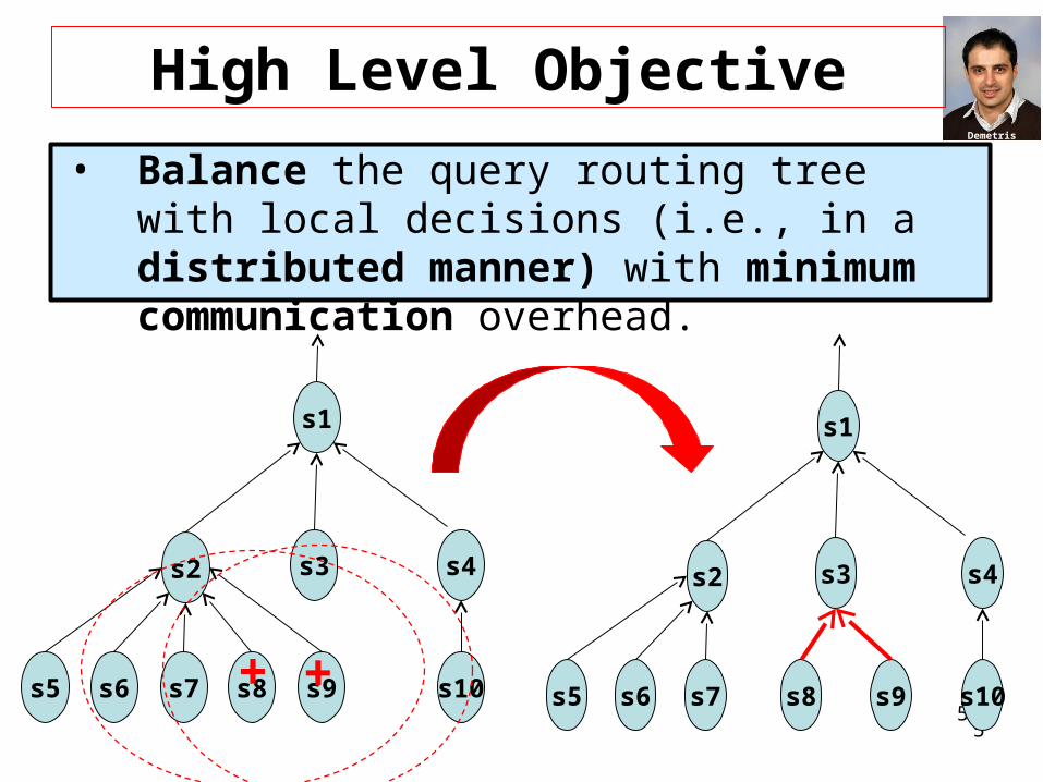
High Level Objective
• Balance the query routing tree with local decisions (i.e., in a distributed manner) with minimum communication overhead.
5s5
s1
s3s2 s4
s6 s7 s8 s9 s10 s5
s1
s3s2 s4
s6 s7 s8 s9 s10++

Demetris Zeinalipour
6
Presentation Outline
Motivation Definitions & Background The MHS Framework
• Dissemination Phase• Parent Selection Phase
Experimentation Conclusions & Future Work
Demetris Zeinalipour
7
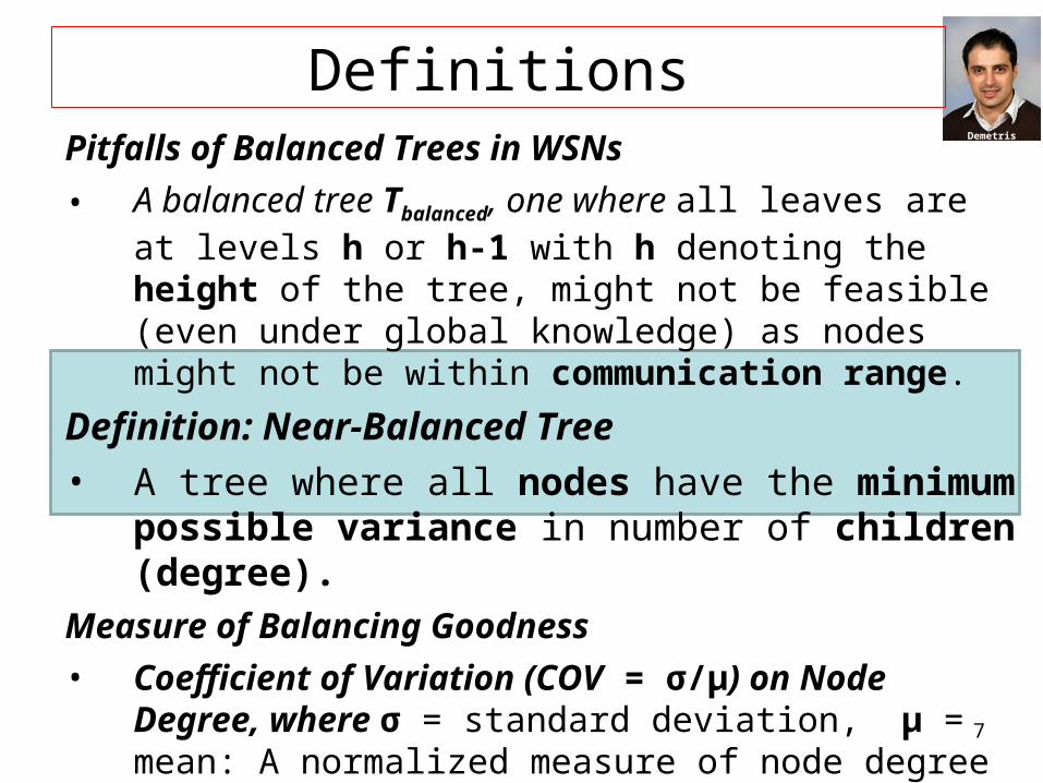
DefinitionsPitfalls of Balanced Trees in WSNs
• A balanced tree Tbalanced, one where all leaves are at levels h or h-1 with h denoting the height of the tree, might not be feasible (even under global knowledge) as nodes might not be within communication range.
Definition: Near-Balanced Tree
• A tree where all nodes have the minimum possible variance in number of children (degree).
Measure of Balancing Goodness
• Coefficient of Variation (COV = σ/μ) on Node Degree, where σ = standard deviation, μ = mean: Α normalized measure of node degree dispersion.
• Low COV is good (as it implies that the variation in degree is low, thus balancing is high)

Demetris Zeinalipour
8
Background: The ETC Algorithm• ETC* (Energy-driven Tree Construction), a
framework for balancing arbitrary query routing trees in an in-network and distributed manner.
• Basic Idea: Attempt to provide each node with approximately β = ⌊d√n⌋ children nodes.
• ETC Basic Phases:– Phase 1: Discover the network topology.– Phase 2: Distributed Network Reorganization.
• Visual Intuition presented next … * P. Andreou, A. Pamboris, D. Zeinalipour-Yazti, P. K. Chrysanthis, G. Samaras, "ETC: Energy-
driven Tree Construction in Wireless Sensor Networks'', In SeNTIE'09, with MDM'09.
“Optimized Query Routing Trees for Wireless Sensor Networks", P. Andreou, D. Zeinalipour-Yazti, A. Pamboris, P. Chrysanthis, G. Samaras, Information Systems (InfoSys), Elsevier, June 2010.
Demetris Zeinalipour
9
ETC: Discovery Phase
s5
s1
s3s2 s4
s6 s7 s8 s9 s10
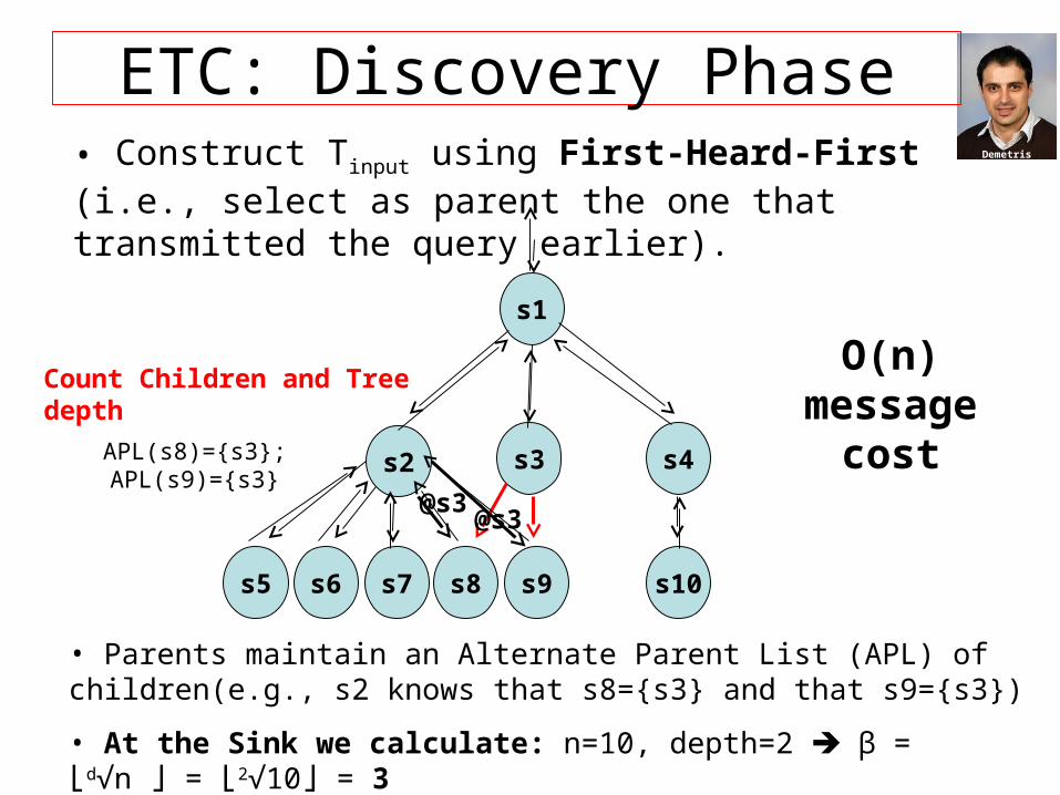
• Construct Tinput using First-Heard-First (i.e., select as parent the one that transmitted the query earlier).
@s3@s3
• Parents maintain an Alternate Parent List (APL) of children(e.g., s2 knows that s8={s3} and that s9={s3})
• At the Sink we calculate: n=10, depth=2 β = ⌊d√n ⌋ = ⌊2√10⌋ = 3
O(n) message
costAPL(s8)={s3}; APL(s9)={s3}
Count Children and Tree depth
Demetris Zeinalipour
#s3 #s3
10
ETC: Balancing Phase
s5
s1
s3s2 s4
s6 s7 s8 s9 s9
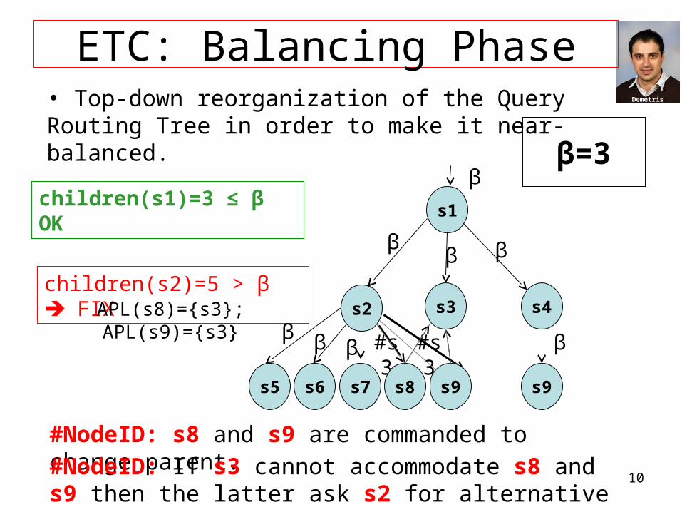
• Top-down reorganization of the Query Routing Tree in order to make it near-balanced.
children(s1)=3 ≤ β OK
children(s2)=5 > β FIX
β=3
βββ
β
APL(s8)={s3}; APL(s9)={s3}β β β
#NodeID: s8 and s9 are commanded to change parent.
β
#NodeID: If s3 cannot accommodate s8 and s9 then the latter ask s2 for alternative parents.

Demetris Zeinalipour
11
Background: The ETC Algorithm
Drawbacks of ETC1. ETC is based on the global branching
factor β of the Tree, which works well in uniform degree distributions (i.e., all nodes approx. same number of children) but not well in random degree distributions.
2. Although better than a centralized algorithm, ETC might add significant communication overhead in order to balance the Tree (especially in the 2nd step)

Demetris Zeinalipour
12
Presentation Outline
Motivation Definitions & Background The MHS Framework
• Dissemination Phase• Parent Selection Phase
Experimentation Conclusions

Demetris Zeinalipour
13
The MHS Framework• MHS stands for Minimum-Hot-Spot Trees Basic Idea: Balance the query routing tree level-
by-level, by having nodes snoop the choices of neighboring nodes. (i.e., purely distributed)
MHS has 2 phases:– Phase 1: Disseminate the Query– Phase 2: Parent Selection by Snooping.
• Visual Intuition behind algorithms will be presented next …

Demetris Zeinalipour
14
MHS Phase 1: Dissemination
A) Disseminate Query
B) Count Parents: Children count their candidate parents.
C) Set Timeout: Use ordering to set a timeout for each node that is proportional to the number of candidate parents (i.e., if more parents => choose last!)
s5
s1
s3s2 s4
s6 s7 s8 s9 s10
APL(s9)= {s2,s3,s4}
Conceptual Order of Parent Selection1)s5, s6 and s10 (AP=1)2)s7, s8 (AP=2)3)s9 (AP=3)
Demetris Zeinalipour
15
MHS Phase 2: Parent Selection
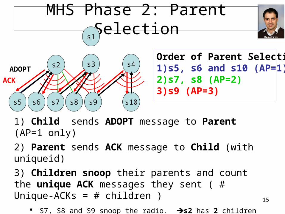
1) Child sends ADOPT message to Parent (AP=1 only)
2) Parent sends ACK message to Child (with uniqueid)
3) Children snoop their parents and count the unique ACK messages they sent ( # Unique-ACKs = # children )
• S7, S8 and S9 snoop the radio. s2 has 2 children while s4 has 1 child.
4) Next order nodes select parent with the min # of ACKs• i.e., first s8, then s7 (rand. delta delay, like TDMA, provides ordering)• finally s9 selects s4 as parent.
s5
s1
s3s2 s4
s6 s7 s8 s9 s10
Order of Parent Selection1)s5, s6 and s10 (AP=1)2)s7, s8 (AP=2)3)s9 (AP=3)
ADOPT
ACK
Demetris Zeinalipour
16
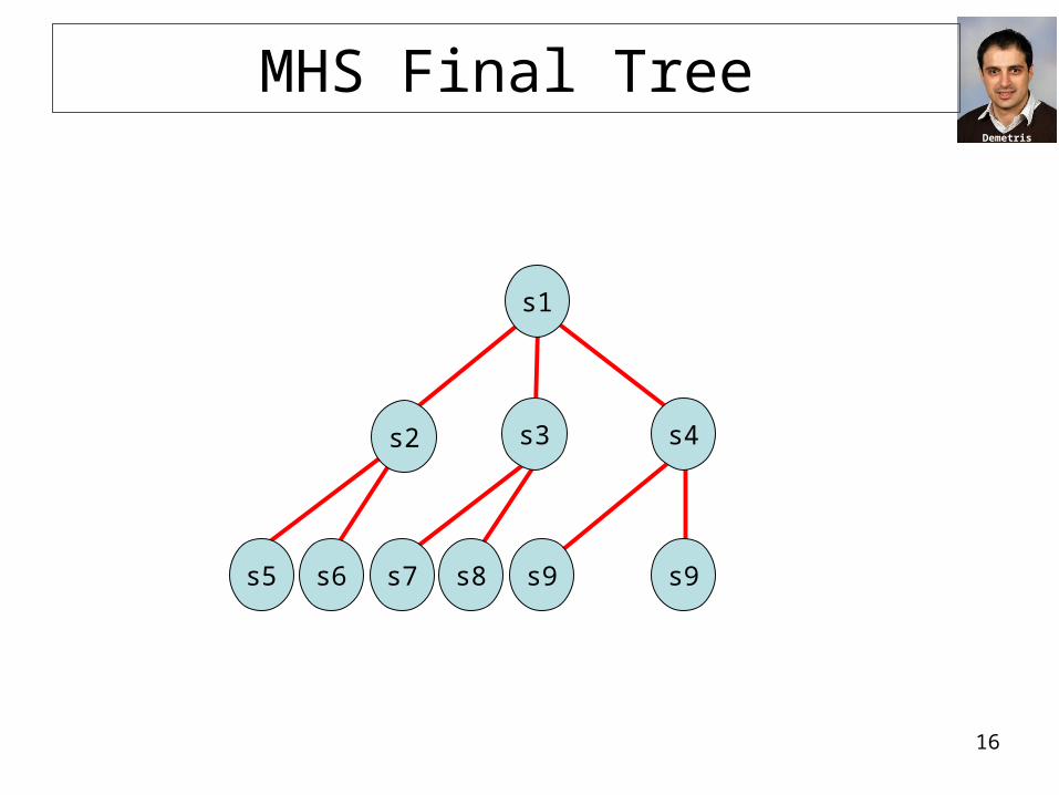
MHS Final Tree
s5
s1
s3s2 s4
s6 s7 s8 s9 s9

Demetris Zeinalipour
17
Presentation Outline
Motivation Definitions & Background The MHS Framework
• Dissemination Phase• Parent Selection Phase
Experimentation Conclusions
Demetris Zeinalipour
18
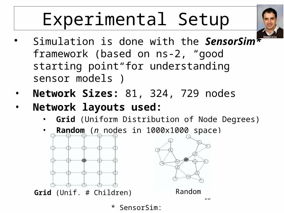
Experimental Setup Simulation is done with the SensorSim* framework
(based on ns-2, “good starting point for understanding sensor models”)
• Network Sizes: 81, 324, 729 nodes• Network layouts used:
• Grid (Uniform Distribution of Node Degrees)• Random (n nodes in 1000x1000 space)
Random
* SensorSim: http://nesl.ee.ucla.edu/projects/sensorsim/
Grid (Unif. # Children)

Demetris Zeinalipour
19
ExperimentsCompared Algorithms1. COPT: Centralized OPTimal algorithm that constructs an
optimally balanced query routing tree.
2. ETC: Balancing based on the global branching factor β
3. MHS: Our proposed algorithm, level-wise balancing based on parent selection snooping.
Evaluation Metrics: Balance Quality: Node Degree Coefficient of Variation
COV = σ/μ , where σ = standard deviation of node degree, μ = mean value of node degree
Energy Consumption: measured in Joules

Demetris Zeinalipour
20
Experiment: Balancing Quality(Grid Network)
81 324 729 # of nodes
a) MHS and ETC are only slightly worse than COPT (i.e., 0.16 COV on average)
b) ETC performs better than MHS for larger networks (β performs well in uniform dist.)
Grid network

Demetris Zeinalipour
21
Experiment: Balancing Quality(Random Network)
81 324 729 # of nodes
a) MHS only marginally worse than COPT (optimal) and better than ETC (i.e., by 0.5 COV)
Random Network
Demetris Zeinalipour
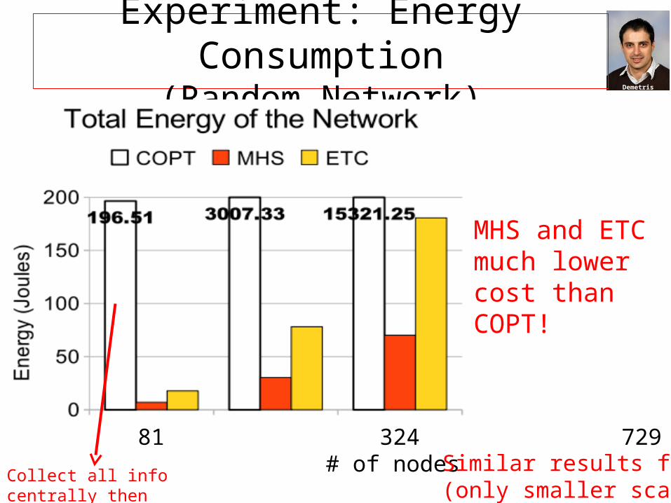
Experiment: Energy Consumption(Random Network)
81 324 729 # of nodes Similar results for grid
(only smaller scale)
MHS and ETC much lower cost than COPT!
Collect all info centrally then disseminate solution back
Demetris ZeinalipourMHS: Minimum-Hot-SpotQuery Trees
for Wireless Sensor Networks
Thanks!
Questions?

Demetris Zeinalipour
26
Motivation
[AZP10] “Optimized Query Routing Trees for Wireless Sensor Networks", P. Andreou, D. Zeinalipour-Yazti, A. Pamboris, P. Chrysanthis, G. Samaras, Information Systems (InfoSys), Elsevier Press, June 2010.
• Unbalanced Communication Topologies impose a significant network overhead (i.e., increase in Loss Rate)
• Right: Microbenchmark in TOSSIM that shows how the loss rate increases by increasing the sink degree [AZP10]
Degree of Sink
57%
Demetris Zeinalipour
27
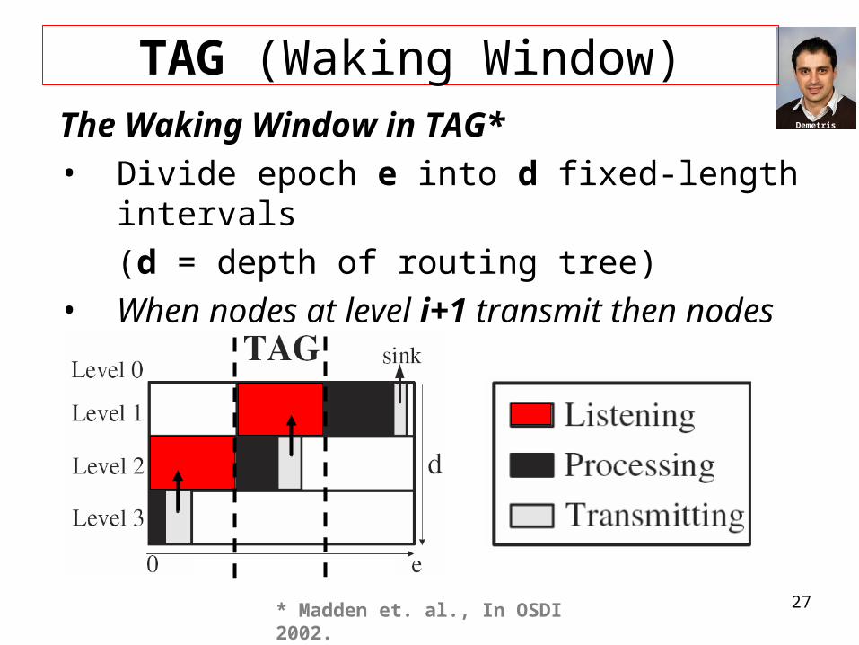
TAG (Waking Window)The Waking Window in TAG*• Divide epoch e into d fixed-length intervals
(d = depth of routing tree)• When nodes at level i+1 transmit then nodes
at level i listen.
* Madden et. al., In OSDI 2002.
Demetris Zeinalipour
28
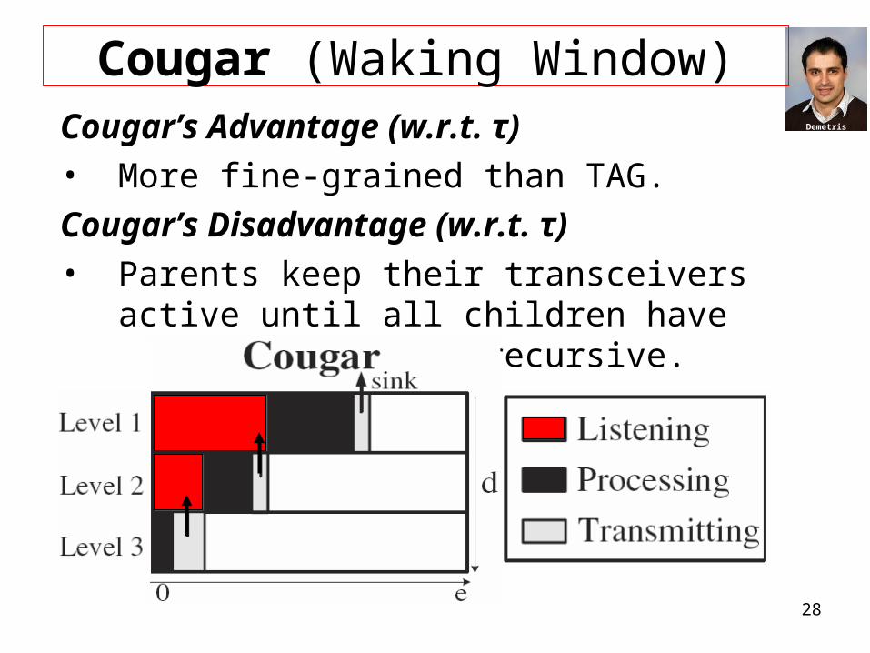
Cougar (Waking Window)Cougar’s Advantage (w.r.t. τ)• More fine-grained than TAG.
Cougar’s Disadvantage (w.r.t. τ)• Parents keep their transceivers active until all
children have answered….this is recursive.

Demetris Zeinalipour
29
A Query Routing Tree in TinyDBExample: The Query Routing Tree in TinyDB• epoch=31, d (depth)=3
yields a window τi = e/d= 31/3 = 10
Transmit: [20..30)Listen: [10..20)
A
C
level 1
B
D E
level 2
level 3
Transmit: [10..20)Listen: [0..10)
Transmit: [0..10)Listen: [0..0)
Demetris Zeinalipour
30
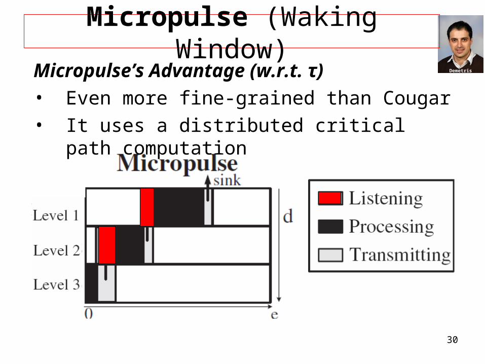
Micropulse (Waking Window)Micropulse’s Advantage (w.r.t. τ)• Even more fine-grained than Cougar• It uses a distributed critical path computation


![Indexing and Searching in Wireless Sensor Networks Demetris Zeinalipour [ zeinalipour@ouc.ac.cy ] School of Pure and Applied Sciences Open University of](https://img.pdfslide.us/doc/110x75/56649e6c5503460f94b6b9b8/indexing-and-searching-in-wireless-sensor-networks-demetris-zeinalipour-zeinalipouroucaccy.jpg)


![MicroHash:An Efficient Index Structure for Flash-Based Sensor Devices Demetris Zeinalipour [ zeinalipour@ouc.ac.cy ] School of Pure and Applied Sciences](https://img.pdfslide.us/doc/110x75/56649eca5503460f94bd8cc0/microhashan-efficient-index-structure-for-flash-based-sensor-devices-demetris.jpg)