Demand system estimation with individual heterogeneity: an analysis using panel data on

households*

José M. Labeagaa

and

Jordi Puigb

First draft: October 1998

This revision: December 2003

Abstract

The main goal of this paper is to assess the importance of controlling individual unobservable effects and measurement errors when analysing demand patterns at the microeconomic level. We provide empirical evidence on the demand for non-durable goods using a panel of households from the Spanish Continuous Family Expenditure Survey. The functional form we adopt is based upon the Almost Ideal Model. We describe how heterogeneity among consumers and measurement errors affect inferences on expenditure and price effects. We cannot reject the presence of correlated unobserved heterogeneity that could bias pooled estimates. In general, income effects show a downward bias and price effects an upward bias. We also describe specific patterns for the bias derived from each source of error, by using suitable instruments.

Keywords: Demand analysis, heterogeneity, panel data.

JEL Class.: C33, D12.

* We wish to thank participants in a seminar at the Centre for Applied Microeconometrics in Copenhagen and specially Martin Browning, Richard Blundell, Jaume García, Bo Honorè, Tsusumu Imai, Angel López, Ian Preston and Eva Ventura for their comments and suggestions. José M. Labeaga acknowledges the hospitality while visiting the CAM and the Ministry of Finance and CICYT projects PB98-1058-C03-02 and BEC2002-04294-C03-02 for financial support. All remaining errors are ours. a UNED, Madrid. b ESCI and Universitat Pompeu Fabra.

1. Introduction

The increasing number of surveys on individual or household data, collecting information

on consumption and also including socioeconomic variables, has raised the interest for

microeconomic consumer behavior. Papers as Blundell (1988), Browning and Meghir

(1991) or Blundell, Pashardes and Weber (1993), among others, show the relevance of

using microeconomic data to approach the analysis of consumer demand. The advantages

of using disaggregated data are mainly that we avoid the problem of aggregation and

therefore its implied bias. However, this sort of information is associated to measurement

errors as well as zero expenditure records, which complicates the estimation. This problem

becomes more important the more disaggregated are the categories of expenditure that we

analyze. Nevertheless, considering data at the household level, we can focus on

idiosyncratic measurement errors, namely, unobserved heterogeneity.

The shortage of data has conditioned very much the empirical work in demand

analysis. The almost exclusive focus on cross-section data for estimating demand systems

could be explained by the limited availability of panel databases or the difficulty for

handling panel data from an econometric point of view. But individuals (households) are

heterogeneous and panel data provide a useful source for testing consumption behaviour

(see Calvet and Comon, 2000). While it is common to use panel when modelling single

goods1, or an aggregate of consumption (see for instance Browning and Collado, 2001), it

is not as usual to do so for estimating complete demand systems (Labeaga, Preston and

Sanchis-Llopis, 2000 and Christensen, 2002, are exceptions). Panel data has obvious

advantages for adjusting individual behaviour regarding demand for commodities. First, we

can control time invariant individual effects. Second, we can estimate dynamic

specifications or use suitable instruments in static ones.

The main goal of this paper is to assess the importance of controlling individual

unobservable effects and measurement error due to infrequency of purchases when

analysing demand patterns at the microeconomic level. Specifically, we produce empirical

evidence on the demand for non-durable goods in Spain, using a panel of households taken

from the Continuous Family Expenditure Survey (ECPF). The functional form we adopt is 1 See Labeaga and López (1997) for a private transport demand equation, or Labeaga (1999) and Jones and Labeaga (2002) for the estimation of rational addiction models of tobacco consumption.

1

based upon the Almost Ideal Model (AIM, Deaton and Muellbauer, 1980) or its Quadratic

extension (Banks, Blundell and Lewbel, 1997). Hence, we are able to analyse how budget

and price changes affect household behaviour. We also try to describe how heterogeneity

among consumers affects inferences on expenditure and price effects.

We concentrate the analysis on the specification and estimation of a demand system

for nine aggregated categories of non-durable expenditure. The analysis of decisions on

those goods is assumed to be independent of decisions on durables and leisure, following

the two-stage budgeting approach (Gorman, 1981). This procedure requires invoking weak

separability. Alternatively, it would be possible to model expenditure on non-durables

conditional on durable decisions and on labour supply (Browning and Meghir, 1991) but

our data does not contain information on either tenure of durable goods and we have

variables relative to the labour status of the head and spouse but the survey does not

provide the number of hours worked by them. In these circumstances, we are forced to

invoke weak separability, except for the inclusion of an aggregate of durable expenditure

and some dummies controlling the labour market status.

In longitudinal data of individuals or households, an important part of the variation

in the consumption pattern of the household can be attributable to individual effects both

observable and unobservable (see Calvet and Comon, 2000 or Christensen, 2002), since the

presence of heterogeneity among individuals is obvious. If this is the case, its control is a

crucial part of the analysis. If this heterogeneity remains relatively constant over time, the

panel structure allows us to control for it. Cross-section analysis cannot either control or

estimate these time invariant effects. The observable effects are measurable specific

characteristics of the household, such as occupational and labour market status and their

inclusion overcomes partly the restriction of the imposed separability between consumption

and leisure. The individual unobservable effects are specific factors for the household units

(differences in tastes) and are assumed to be constant.

The presence of zero expenditure records is quite common when working with

disaggregated categories of expenditure. In this paper, the constructed aggregates, as well

as the treatment of the data, allows us to consider that all zeros can be associated to

infrequency of purchase. This source of zero expenditures has usually been analysed by

introducing the distinction between non-observed desired consumption and observed

expenditure (Keen, 1986). According to this difference, both variables are related through a

2

policy of purchase for each household, which depends on the purchase probabilities.

Usually, these probabilities have been modelled as dependent on socio-economic and

demographic variables.2 We also allow for the presence of errors in variables that are not

explained in terms of infrequent purchases. The distinction between observed expenditure

and desired consumption leads to a relation between observable quantities plus an error in

variables. Considering also the presence of unobservable heterogeneity, correlation

between some regressors and the error structure may arise from different sources.

Nevertheless, given the dependence of the household policy of purchase on family

characteristics and purchase habits, it seems reasonable to think that when controlling for

those individual unobservable effects, we take into account, at least partly, the effects of

infrequent purchases.

We present Ordinary Least Squares (OLS) and Instrumental Variables (IV) results

for different specifications estimated both in levels and first differences. We derive and

compare the income and price elasticity figures from the different models. We confirm that

the presence of correlated heterogeneity bias the pooled estimations. Moreover, we also

describe specific patterns for the bias derived from each source of error, using suitable

instrument for total non-durable expenditure. We find that income effects from pooled

models are downwardly biased for most of the categories of expenditure while price effects

generally present an upward bias.

The rest of the paper contains five sections. Section 2 presents the theoretical

framework in which the analysis is developed. The description of the sample, the treatment

of infrequency and its association to the latent effects are analysed in section 3. Section 4 is

devoted to the econometric methods and section 5 to discuss the results. Section 6

concludes.

2. Modelling framework

2.1. Separability assumptions

The analysis of consumer choices takes into account decisions between consumption and

leisure, as well as the allocation of expenditure over commodities. The study of the

3

2See Meghir and Robin (1991) for an example on a joint model for frequency of purchase and consumer demand. Labeaga and López (1997) argue that in a short time period the purchase policy can be considered a fixed effect. This is obviously a restrictive assumption when a housing change or a change in the composition of the family happens during the period.

disaggregated categories of expenditure implies several complementary and substitutability

relationships. In order to reduce the problem to a tractable one, consumer patterns are

usually analysed for broad groups. The logical approach is that consumption is partitioned

into subsets that include commodities that are closer substitutes or complements among

them. Weak separability has been the usual hypothesis in empirical demand analysis since

it provides an approach for studying broad groups. According to this idea, the marginal rate

of substitution among goods belonging to the same group is independent of any other good

outside the group.

For a utility function V, this assumption allows to write the same preference

ordering:

V( [1] ))c(V),...,c(VF(=)c,...,c nn11n1

being V1 ,..., Vn sub-utility functions, F some increasing function and ci the consumption on

good i.

Weak separability is a pre-requisite for two-stage budgeting. According to the idea

of two-stage budgeting, consumers proceed first to allocate total income among broad

groups. In a second step, consumers decide how to distribute expenditure on individual

goods. If a subset of goods appears in a separable sub-utility function, we can obtain

demand functions for those goods as a function of expenditure on the group and prices of

the different individual goods. In the opposite direction, the existence of a subgroup of

individual demand functions depending only on prices of individual goods included in that

group and on expenditure on the aggregate implies weak separability. The advantages of

this approach are obvious. Since it reduces the original problem to a sequence of decisions,

each step requires only information on prices and expenditure on that specific decision

level. Therefore, the maximization of V requires each ci, depending on the n-prices and

total expenditure, to be the solution for the maximization of each Vi. Although weak

separability is very useful from an empirical point of view, it is not exempt from critiques

as Blundell and Robin (2000) show with the concept of latent separability (see also

Labeaga and Puig, 2002, for some empirical implications of using latent instead of weak

separability). We also invoke along the paper intertemporal separability on preferences so

4

that the distribution of current consumption can be decided independently of the

assignment of life-cycle expenditure.3

We concentrate exclusively on decisions over non-durable goods. Durable goods

require specific models such as stock adjustment or probability of expenditure models. The

analysis of these goods is out of the scope of this paper. Considering only non-durables we

are also assuming separability between consumption and leisure. If leisure is weakly

separable from consumption, decisions on leisure, and therefore on income, will be

independent of the assignment of expenditure. This is a rather restrictive hypothesis.

Browning and Meghir (1991) propose an alternative approach to overcome this problem.

They model demand decisions conditional on hours and participation dummies, which

characterize labour supply. Even though we include some participation variables in a non-

restricted way, we cannot model the suggested reduced form since our data does not

contain information on hours. The number of worked hours may be proxied by

introducing a participation dummies since most of male workers are full-time

employed, although this is not the case for females.

2.2. The Almost Ideal Model (AIM)

We apply this formalization to the AIM of Deaton and Muellbauer (1980) or a quadratic

generalization. Three reasons may qualify this specification for the demand functions. First,

it is a first order approximation to the demand functions that relates expenditure shares for

each good with prices and expenditure with the form:

)PX( log + p log + ijijj βγ∑ = w ii α [2]

where P is a price index defined as:

p log p log 21 + p log + = P log lkkllkkkk0 γαα ∑∑∑ [3]

This functional form is almost linear except for the price index. Most of the

empirical works approximate linearly this function using a Stone price index.4 Since this

5

3 The acceptance of this hypothesis depends very much on the good analyzed and on the period of time of expenditure we consider (see Attfield and Browning, 1985 or Browning, 1991). There is also evidence in microeconomic analysis that supports this hypothesis (Meghir and Weber, 1996). Nevertheless, Carrasco, Labeaga and López-Salido (2002) reject it with data taken from this same survey.

price index enters all equations as a deflator for expenditure, we have a linear estimation

problem. Also, the demand system for our problem is not constrained to expenditure or

income but non-durable expenditure. Thus, the different analyzed goods form a separable

group respect to the durable goods in the budget of the consumer. Our attention focuses in

specifying the second step of a two-step budgeting procedure.

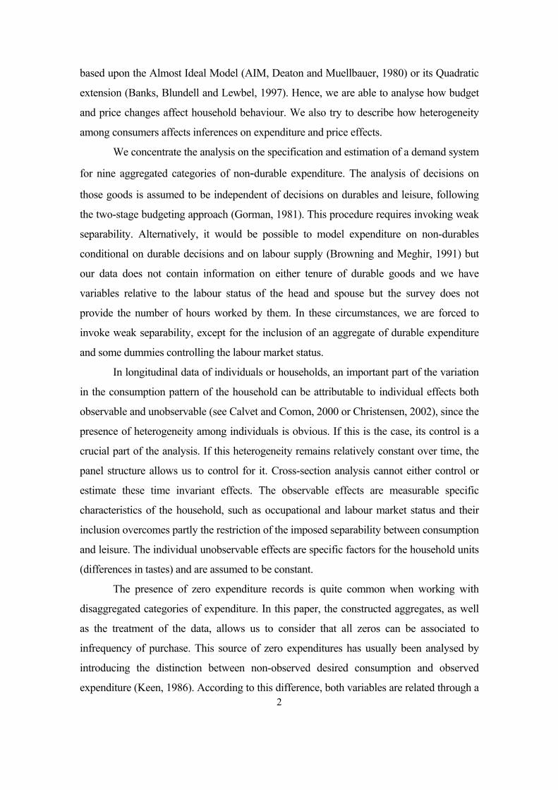
The second advantage is that theoretical restrictions can be imposed and tested very

easily. The unrestricted estimation of the AIM is going to satisfy only additivity to keep full

rank of the system. The rest of conditions will be testable in a simple way via parameter

restrictions. These restrictions are:

. :symmetry

, :y homogeneit

, , , : additivity

ijji

jkk

kkkjkkk

γγ

γ

βγα

=

=∑

=∑=∑=∑

0

001

Thirdly, this functional form is derived from a PIGLOG class of preferences that

permit exact aggregation over consumers. These preferences are characterized by a cost

function that in our case takes the form:

p = b(p) and

p log p log 21 + p log + = a(p) being

,b(p) U + a(p) = p)c(U, log

kkk0

lk*kllkkkk0

βΠβ

γαα ∑∑∑ [4]

where α, β, and γ* are parameters. This is a very flexible specification in terms of the

income and price responses. This model also allows for an easy and flexible inclusion of

demographic and socio-economic variables, which have revealed as significant

determinants of household consumption patterns (see Pollak and Wales, 1981).

Another important issue concerning the demand model is the rank of the system.

Gorman (1981) demonstrates that the rank of the matrix of coefficients for the polynomial

terms in income is at most three. Extending the AIM, which is initially rank two, to a rank

three specification we obtain the following functional form:

4 We define log Ph = Σi wih log pi, being wih the budget share of good i for household h. Pashardes (1993) shows that using such approximation, price effects estimates on the AIM may display parameter bias specially if applied to individual data. Nevertheless, this bias depends mostly on the correlation between the expenditure parameters and the intercepts in the budget share equations. Estimations in first differences will overcome this inconvenient.

6

))PX(log( + )

PX( log + p log + = w 2

iijijjii δβγα ∑ [5]

which is the simplest quadratic extension of PIGLOG demands. Notice that integrability for

a demand system with the above form requires δI = β i* ε for all categories of expenditure.5

Although this is a very simple extension, it will allow us to detect up to what point a rank

two specification is too restrictive to impose on our data. However, this non-integrable rank

three model is regularly used in practice (see Blundell, Pashardes and Weber, 1993 or

Labeaga and López, 1996), whenever we are not interested in welfare analysis.

3. Sample design

3.1. Description of the sample

The sample used in this paper comes from the ECPF. This is a quarterly survey conducted

by the Instituto Nacional de Estadística (INE, 1985) since 1985. The sample we work with

covers the period 1985-1991. The survey established the interview of households

throughout 8 quarters. Thus, the original design implied a rate of substitution of 1/8. Data

analysis shows that there exists a higher level of attrition, which leads to a higher rate of

substitution and fewer observations per household. Therefore, the actual sample is an

unbalanced panel in the sense that we do not have the same number of temporal

observations for each household. If families leave the survey according to a specific

pattern, non-random attrition will imply biased and inconsistent estimates. Nonetheless,

representativeness is preserved throughout all the considered period and hence, we may

think that attrition is random concerning the estimation of demand functions.

When working with microeconomic data, we must deal with an important the

problem of zero records on several categories of consumption. This constitutes an

important justification for grouping goods. Several reasons may generate zero

expenditure: first, as a result of a corner solution; second, non-participation; third,

infrequency of purchase. We can add missreporting or individual effects. The nature of

observed zeros depends very much on the category of expenditure we consider. As

5 An integrable Quadratic Almost Ideal Demand System that did not verify such a condition might be formulated as suggest Banks, Blundell and Lewbel (1997):

∏=

∑N

ik

kp = b(p) being,)))p(fX(log( b(p))/ ( + ))p(f

X( log + p log + =w 2iijijjii

1

βλβγα

7

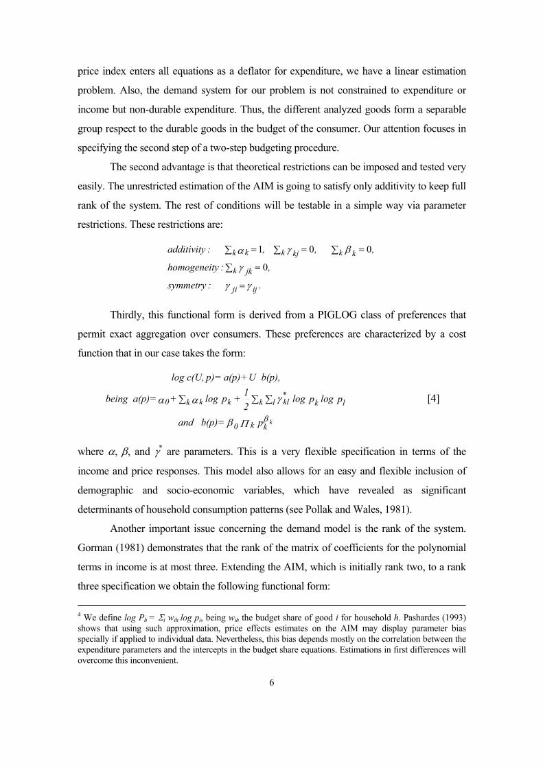
suggested by Blundell and Meghir (1987a), a suitable assumption is that there is only

one source of zeros for each good. However, categories with zeros mainly due to non-

participation require specifications that include the participation decision. A conditional

demand system is the most suitable framework to model demands on these goods.6

Since we are interested in evaluating the potential biases that infrequent purchases

might generate, we restrict our attention to goods for which infrequency of purchase can

be reasonably assumed to be the unique source generating zeros. In this sense, we do

not explicitly model tobacco and petrol.

We select 9 groups of expenditure on non-durables. These groups do not cover total

expenditure on non-durables since we exclude consumption on those goods for which

expenditure may be conditional on participation variables. The expenditure goods we

consider are: food and non-alcoholic beverages, alcoholic beverages, clothing and

footwear, rents and house keeping expenditures, fuel for housing, transport and

communications, services and leisure expenses, household non-durables and other non-

durable goods.

The final sample we work has 4372 households observed throughout 6 quarters. It

has been selected according to two criteria: first, we maintain those households that stay at

least 6 quarters. A cohort analysis shows that none of the households that enter the survey

in 1985 and the first 3 quarters of 1986 complete the 8 quarters. Selecting only those

households that respond 8 quarters, we loose representativeness of an important period in

terms of price variation. Moreover, most of the families stay in the survey 6 quarters or

less. In order to have a balanced panel we drop the last two observations for those

households who report 8 quarters and the last one for those that report 7. This temporal

profile gives enough lags of the variables that may be used as instruments.

The second sample selection criterion is that we require consumption participation

on the goods analysed. Panel data allows the identification of zeros due to non-

participation. We assume that a single non-zero expenditure observation throughout the

observed period identifies the household as a consumer on that group. By doing so, we

associate the remaining zero expenditures to infrequency of purchase. For food and non-

alcoholic beverages we require expenditures to be positive in every quarter.

8

6 See, for instance Lee and Pitt (1986). These approaches are not feasible when analyzing more than 3 goods.

3.2. Infrequency of purchase

Infrequent zeros arise due to the indivisibility of expenditure in such a way that the specific

moment of purchase does not fall within the monitoring period covered by the survey (that

is a week for most of the good we model). Moreover, infrequency can also be due to

searching costs. In the absence of these costs (or highly storage costs) and perfect

divisibility, consumers would distribute their expenditure in such a way that household

desired consumption would coincide with observed expenditure whatever the period we

considered.

The framework we consider to analyse infrequency of purchase is based on the

differentiation between desired non-observed consumption chk and observed real

expenditure ehk for household h on good k (Kay, Keen and Morris, 1984 and Blundell and

Meghir, 1987b). The stochastic relationship among both takes the form:

[6] u +pr / } c{ hkhkhkhkd = ehk

where uhk is an error; dhk is a random variable distributed as a Bernouilli and prhk, is the

probability of purchase of good k by household h during the interview period. Two sources

of measurement error come up from this distinction. The purchase decision implies an error

that explains itself the presence of zeros. The implied consequence is that real observed

expenditures are biased estimators of desired consumption. The usual approach has been to

instrument expenditure with income as proposed by Keen (1986). This procedure does not

require the knowledge of the purchase probabilities. Also, we introduce the possibility that

observed real expenditure does not coincide with desired consumption due to other

circumstances different than infrequency. Considering this model, we take into account

both the effects of the household purchase policy and other errors in variables which are

not determined by infrequent purchases.

Meghir and Robin (1991) suggest a method to deal with unobserved consumption

that takes into account the purchase probabilities and also allows to deal with non-linear

models. The suggested procedure requires obtaining those probabilities of purchase over

the whole sample, conditional on demographic characteristics. In a second step, those

households that have positive expenditures are selected and desired consumption is

constructed for them by re-weighting observed expenditures with the estimated

probabilities. Working with a panel data, this approach implies a high cost in terms of the

9

number of observations we loose since the selection of positive expenditures will withdraw

those households for whom continuous in time observations are not available.7

The distinction between observed expenditure and desired non-observed

consumption according to equation [6] for the AIM leads to a stochastic relationship with

the form:

qp

qp =

u +pr/ } qp{du +pr/ } qp{d

*hktktk

*hktkt

hktkhkhktkthkk

hkthkhktkthk

∑∑∑ [7]

being pktqhkt* and pktqhkt observed and desired expenditure for period t on good k by

household h. As pointed out, the purchase policy is modelled through the probability of

observing a positive expenditure and the dummy variable. Notice that we assume that both

are time invariant since these probabilities are assumed to be dependent on household

characteristics. Since it is not usual to observe important changes coming along in six

quarters, we propose a time invariant purchase policy. Introducing this purchase policy into

the demand equations, we obtain the following relationship between observables:

ηεα

ββγα

hkthkthk

tkhktkhk

hk*hktkt

kkjtkjk*hktktk

*hktkt

+

+ p ln - ])u-d

pr* qp[ ln(+p ln+=

qp

qp

+

∑∑∑∑ [8]

being .qp

qp -

u +pr/ } qp{du +pr/ } qp{d

= hktktk

hktkt

hktkhkhktkthkk

hkthkhktkthkhkt ∑∑∑

η

We also include the parameters αhk, which represent the individual unobserved

effects. Notice also that we are considering time variant errors in variables for expenditure

on each individual category and for total non-durable expenditure. Moreover, the error

structure has been derived accounting also for errors in variables in the left-hand-side. As

far as the error in variables occurs in a specific good, no special problem comes up.

However, since the denominator is total expenditure, under a problem of errors in variables,

it has a non-polynomial structure and no obvious solution exists. We recall Hausman,

Newey and Powell (1995). They do not find significant differences specifying the 7 The number of periods we observe a household purchasing could be used as the purchase probability to apply the method proposed by Meghir and Robin (1991). Labeaga and López (1997) apply this method as

10

dependent variable in levels and in budget shares when estimating Engel curves. This

empirical evidence is used to assess that the errors in variables in the denominator of the

left-hand-side variable in a budget share specification do not create an important problem.

Therefore, omitting this source of error and assuming a linear structure we can account for

an instrumental variables estimation procedure and the above expression becomes:

qp

qp -u + pr/] qp[ d = hktktk

hktkthkthkhktkthkhkt ∑

η [9]

Appending [9] to the error, we can write its complete structure as:

hkthkt + w1 εεqp

u + prd

= hktktk

hkt

hk

hkhkt

∑

−η + hkt

[10]

The first component collects information about the purchase policy. In fact, it

consists of an interaction between the policy of purchase and the desired budget shares.

Notice that the latter depends on prices and total non-durable desired expenditure and

hence, it displays individual and time variation. Besides, the probabilities of purchase are

usually assumed to be dependent on household characteristics. Under these circumstances,

we may conclude that the error component related to the policy of purchase must affect all

categories of expenditure in the same way. The second term refers to errors in variables

different than those generated by infrequency, while the third corresponds to the usual

stochastic term. Notice that we do not include time specific components since the data has a

reduced temporal span and we will capture their effects by time dummies.

Correlation between this error structure and the regressors is obvious. The implied

inconsistency may come up from correlation between total expenditure and infrequency

and from the errors in variables component. As pointed out, the derived effect from

infrequency of purchase must be the same on all expenditure categories. However, the

direction of the implied bias from correlation between expenditure and errors in variables is

not well determined. Additionally, we must add another source of bias derived from the

potential correlation between individual unobserved effects and the regressors. Considering

the different sources of inconsistency, we can predict that the direction of the bias will not

be the same for all categories of expenditure. OLS estimates will be affected by all these

11

well as a model where the purchase policy is captured by the fixed effects to the estimation of a petrol demand equation.

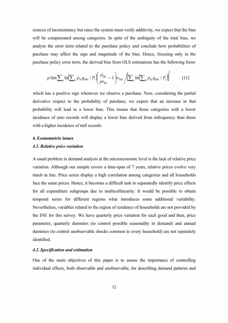
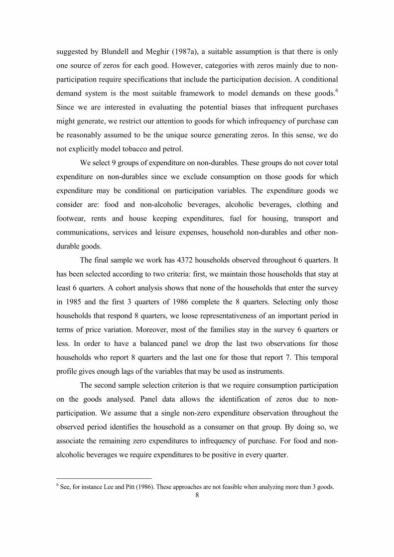
sources of inconsistency but since the system must verify additivity, we expect that the bias

will be compensated among categories. In spite of the ambiguity of the total bias, we

analyse the error term related to the purchase policy and conclude how probabilities of

purchase may affect the sign and magnitude of the bias. Hence, focusing only in the

purchase policy error term, the derived bias from OLS estimations has the following form:

( ) ([ ])2

/ln1/lnlim ∑ ∑∑ ∑

−

n k thktkthkthk

hkn k thktkt Pqpw

prdPqpp [11]

which has a positive sign whenever we observe a purchase. Now, considering the partial

derivative respect to the probability of purchase, we expect that an increase in that

probability will lead to a lower bias. This means that those categories with a lower

incidence of zero records will display a lower bias derived from infrequency than those

with a higher incidence of null records.

4. Econometric issues

4.1. Relative price variation

A usual problem in demand analysis at the microeconomic level is the lack of relative price

variation. Although our sample covers a time-span of 7 years, relative prices evolve very

much in line. Price series display a high correlation among categories and all households

face the same prices. Hence, it becomes a difficult task to separatedly identify price effects

for all expenditure subgroups due to multicollinearity. It would be possible to obtain

temporal series for different regions what introduces some additional variability.

Nevertheless, variables related to the region of residence of households are not provided by

the INE for this survey. We have quarterly price variation for each good and then, price

parameter, quarterly dummies (to control possible seasonality in demand) and annual

dummies (to control unobservable shocks common to every household) are not separately

identified.

4.2. Specification and estimation

One of the main objectives of this paper is to assess the importance of controlling

individual effects, both observable and unobservable, for describing demand patterns and

12

derive expenditure and price elasticities. According to the points considered above, the

final expression for the specification of the demand equation is:

hkthktkt

hktktNjtkjkjkhkt )

PX(+pp +=w ευαλβγα +++∑ hkh +Zlog/log [14]

where αhk captures unobserved heterogeneity and νhkt is the error term related to

infrequency of purchase.

There are several econometric techniques that, applied on panel data sets, control

for unobserved heterogeneity among individuals. The treatment of these latent effects either

as fixed or random does not imply any gain in terms of specification. Working with

samples with a wide cross-section variation, it is desirable to make unconditional

inferences to the sample and therefore, to treat individual unobservable effects as random.

This assumption implies that error terms will have a mixed structure. The GLS estimator

(Balestra and Nerlove, 1966) is going to be consistent and efficient under the hypothesis of

absence of correlation between regressors and errors.

However, when using individual data it is quite usual to detect the presence of

correlation between the error and the regressors. In our analysis, this correlation may arise,

first of all, from the individual unobservable effects and expenditure since the former can

be described as a function of the latter. Estimating equations in levels, we do not remove

these individual unobservable effects and therefore we should detect presence of

correlation. The usual treatment for this problem is to instrument expenditure. An available

straightforward instrument under two stage budgeting seems to be income, which is highly

correlated with expenditure. Nonetheless, this instrument may also be correlated with

unobservable heterogeneity. Notice that using income as instrument we do not take into

account the invariant nature of the latent effects. Other possible invariant in time

instruments refer to characteristics of the family, but they are usually included in the

equation as observable individual effects and then there are identification problems. This

problem may be overcome by using as instruments the individual means of those variables

that are not correlated with the latent effect (Hausman and Taylor, 1981). In our case, we

do not have any regressor uncorrelated with the effects which is variable across individuals

and time. Moreover, correlation between the observable and unobservable individual

effects is expected. For this sort of correlation we do not have any available instrument

13

since these effects are time invariant. If they were not, first differences of the socio-

economic variables could be suitable instruments although sometimes they do not produce

good results.

Finally, another possibility to deal with the presence of time invariant individual

random effects, which are correlated with the regressors, is to remove them by taking first

differences. Estimating by OLS the equations in first differences, we can obtain consistent

estimators, given the static nature of the specification under the assumption of exogeneity

of total expenditure. In fact, dealing with regressors linearly correlated with the latent

effects, the optimal estimator (Minimum Distance or Maximum Likelihood estimator)

coincides with the OLS estimator applied to equations in first differences (Chamberlain,

1984). In fact, if we are dealing only with unobservable effects, the within-groups (WG)

procedure will also provide consistent estimators.

The above analysis has only taken into account correlation between the individual

latent effects and the regressors. We settled the distinction between unobserved

consumption and observed expenditure. From this difference, we deduced the presence of

time dependent errors derived from infrequency. We also considered the presence of

measurement errors in variables. Once more, the implied bias can be solved by

instrumenting those variables from which correlation arise. Again, non-durable expenditure

may be proxied with income. Nonetheless, income may be correlated with infrequency of

purchase since probabilities of purchase mainly depend on household specific variables.

First differences of non-durable expenditure lagged one period may be a suitable

instrument for the estimation in levels if the infrequency errors are i.i.d. Equations in

differences, again under the null of uncorrelated measurement errors, will display first

order but not second order serial correlation. In this case, differences of expenditure lagged

two or more periods will be orthogonal to the first differences errors. Note that if errors of

measurement have a time invariant nature, they will be dropped out in the first differences

estimation and hence, we will not need to use instrumental variables techniques (see the

discussion in Labeaga and López, 1997, in the context of a single demand equation).

Income is the usual instrument either if there is correlation between individual

effects and expenditure or in the presence of error measurement due to infrequency.8 As

14

8 Income appears regularly as underestimated in databases at the microeconomic level and the ECPF is not an exception. Expenditure may come up as misreported as well but this is already captured by the error

pointed out, dependence of the probabilities of purchase on socio-economic characteristics

may translate into correlation between income and infrequency. Moreover, it is worth to

mention that income is going to be a meaningful instrument only if we accept weak

separability between consumption and leisure. If this is the case, the decision on leisure,

and therefore on income, can be considered exogenous related to the consumption on non-

durable goods. Summers (1959) and Liviatan (1961), among others, assume that income is

uncorrelated with the error term associated to a linear Engel curve. Their assumption is

based on the Friedman assessment that permanent income and transitory consumption are

uncorrelated. Under the null of absence of correlation between income and the stochastic

disturbance, a test of exogeneity of expenditure can be derived. Opposite, Attfield (1978)

points out that this is a very strong assumption working with individual data. Household

data will display a high correlation between income and specific unobservable effects. In

this case, possible alternative instruments are lags or leads of expenditure.

For the rank three model, we specify the simple quadratic extension [5]. Working in

a non-linear context and in the presence of measurement errors, the IV procedure will not

provide consistent estimates whatever set of instruments we use (Amemiya, 1985 or

Hausman, Newey and Powell, 1995). The reason has to be found in the fact that the

measurement error is not separable from the true variable. Nevertheless, if this error term is

time invariant, first differentiation will cancel it and despite of the non-separability

structure, the observed regressor will not be correlated with the error in first differences. If

it varies with time, we can still use the Hausman, Newey and Powell (1995) repeated

measurement procedure.9

5. Results

5.1. Discussion upon rank two and rank three specifications

Estimations in levels, either considering data as a pool (OLS), or introducing the presence

of random heterogeneity (GLS) generate certainly different results from those obtained in measurement term. Nevertheless, underestimation of the former exceeds the latter, specially considering that most of the samples, including ours, are designed in order to study the structure of expenditure. Therefore, we must cast doubts about the adequacy of income as a proxy for expenditure.

15

9 This technique proposes to use alternative variables to construct adjusted expenditure, and use it as instrument. Possible variables are education and age which proxy expenditure and will not be correlated with the non-linear stochastic disturbance. Other possible instruments are lagged expenditure or even future expenditure. Under rational expectations, observations located in the following future will be independent of current information and will also proxy current consumption.

estimations in differences (either WG or first differences). We first present an F-test for the

presence of individual effects, which rejects the null of homogeneity (see Table 3).

According to these tests, we need to take account of individual unobservable effects. This

also suggests that their presence could bias the estimations in levels whenever these effects

are correlated with the regressors. We perform a Haussman test to detect more formally the

presence of correlation between individual effects and regressors by comparing GLS and

WG estimators. Notice however that the former will only be consistent under the null of

absence of measurement errors while consistency of the WG estimates requires time

invariant measurement errors. Still, the hypothesis of absence of correlation is rejected for

all the equations. The presence of latent heterogeneity as well as measurement errors from

any source will require to instrument expenditure.

First, we present results of estimations in levels by OLS including as explanatory

variables socio-economic characteristics of the household. They refer to the labour situation

and activity of the head of the household (dummies for non active, self-employed or

unskilled workers), the number of members of the family, number of members under 14

years old and number of earners. We also include 3 quarterly dummies to capture possible

seasonality in consumption. Columns 1 and 2 in Tables A.3 through A.10 report OLS

results, those in column 1 are obtained without instrumenting total expenditure while

column 2 presents results using the lag of total non-durable expenditure (in first

differences) as well as first differences of the mentioned characteristics of the household as

instruments for total non-durable expenditure.

As a general pattern for all estimations, most of the price parameters turn out to be

non-significant, whereas the quarterly dummies are highly significant. Although some of

the coefficients are non-significant, the own price elasticities derived from the values fall

within the expected range and are significantly different from zero (standard errors are

calculated by bootstrapping). Moreover, these price effects are jointly significant for most

of the categories (see tests on Table 3 and Tables A.3 to A.10). We are analysing a period

of 28 quarters; for this short period, the price variation is small, and we also detect a high

correlation between the different price series. Partly, the variation of the relative prices

might be associated to seasonality but the quarterly dummies already pick up this effect.

So, we are capturing disaggregated price effects with a small time series variation. The

parameters for quarterly dummies characterize perfectly seasonality, especially on those

16

categories that follow a different consumption pattern depending on the quarter. When we

do not introduce quarterly dummies, price effects are significant, but their sign and

magnitude are in many cases counterintuitive. On the other hand, parameters corresponding

to total expenditure are estimated with precision as is usual with this kind of data. Their

sign and magnitude are in accordance with a priori expectations, as we will see below.

Socio-economic variables are highly significant for the OLS estimation. The relevance of

these variables for the IV estimation depends on the category of expenditure we analyse.

Labour variables do not seem to affect very much in none of the categories. However,

family composition comes up as very significant on all equations, especially on luxury

goods.

Going to estimations in first differences, column 3 in Tables A.3 to A.10 show OLS

estimates, column 4 present IV coefficients using the second lag of differentiated

expenditure as instrument for total expenditure while column 5 report coefficients using

income as instrument for total expenditure. Since first differentiation implies dropping out

all the variables without time variation, we do not include the socio-economic variables.

We analyse changes in these variables along the 6 quarters and we observe that most of

them show small variation along time (see Table A.1). Price effects are, as above, non-

significant for approximately 50 per cent of the coefficients, whereas total expenditure

effects are well defined. Again, a specification with price variables and without quarterly

dummies raises very much the significance of the former, but instead, the derived

elasticities present some non-intuitive values, because most of the price variation is

captured by seasonality.

Results in column 3 controls for unobserved heterogeneity, but they do not take into

account the possible correlation between first differences of the infrequency error term or

other errors in variables and differences of total expenditure. A test on the comparison of

both sets of instruments provides information about the possible correlation of expenditure

and measurement errors, which is an indirect diagnostic about the endogeneity of

expenditure. Notice first that the results obtained are very similar both for income and price

effects. The value of the Hausman test is 0.01 that must be compared with a χ2 with 96

degrees of freedom. So, we do not reject the absence of correlation among differences of

expenditure and measurement errors. However, since they are correlated in the levels

equations, measurement errors may not be time dependent and hence, they cancel out in the

17

first differences specifications. The same conclusion can be derived if we compare both

sets of estimates with WG coefficients.10

We now turn to a levels specification using first differences of lagged expenditure

as instrument for total expenditure (column 2). If the measurement error structure is i.i.d.,

orthogonality between the proposed instrument and the error components is ensured; hence,

any difference must be explained in terms of correlation between the individual effects and

the regressors. We observe that estimators in the levels equations by OLS (column 1) are

quite close to estimators in the first differences equations by IV (column 2), although the

former are relatively downwardly biased except for housing and domestic fuel. On the

other hand, price effects seem to be upward biased. If we use first differences of income

instead of expenditure (not reported here either), we obtain very similar results. This

supports that correlation between measurement error and differences of expenditure is not

very relevant. Once more, this supports that measurement errors may be time invariant, but

differences in tastes matter.

The specification in levels, without controlling for any source of error, implies

correlation between expenditure, individual effects and/or measurement errors. We now try

to describe the direction of the bias implied from the former source of correlation, by

comparing consistent estimates on column 4 with OLS pooled estimates in column 1. We

observe that the direction of the bias implied only from measurement errors depends on the

category of expenditure. We detect an upward bias on housing, domestic fuel, services and

house non-durables and a downward bias for the rest. As we outlined previously, the

expected bias from the household policy of purchase has an upward effect on the

parameters, especially on those categories with a higher incidence of zeros. This pattern is

only followed by 4 of the analysed categories from which only house non-durable

expenditure is significantly affected by the presence of zero records. Hence, we conclude

that there are also errors in variables or unobserved heterogeneity, different than errors

arising from infrequent purchases, included in the error measurement structure, which bias

the results in the opposite direction.

Back to IV estimations in first differences, if instead of lagged differences of total

expenditure, we use differences on income (column 5), we also control for unobservable

heterogeneity, but we do not take into account either the possible correlation between

1810 These results are not reported here but they are available upon request.

income and infrequency of purchase. Nevertheless, from the previous results we deduce

that measurement errors display an invariant in time nature and hence they cancel out in

this specification in first differences. Comparing both OLS and IV estimators, using income

as instrument for expenditure, all in first differences, we obtain again a test for endogeneity

of total expenditure. This test can also be reinterpreted as a test for the validity of income as

instrument, that is, a test on weak separability. We obtain a value of 4.96, which must be

compared with a χ2 with 96 d.f. This result implies a non-rejection of income as a suitable

instrument. Nonetheless, if we perform the same test only upon the subset of expenditure

parameters, this value raises up to 55.3 (8 df), which clearly rejects the null. As pointed out,

the hypothesis of orthogonality between the stochastic disturbance, εikt, and income seems

questionable when working with data at the individual level. This result could be due either

to measurement errors correlated with income but it could also constitute evidence of non-

separability between consumption and leisure.

We finally present rank three estimates of equation (5). Under time invariant

measurement errors, maximum likelihood (ML) estimation of (5) in first differences will

provide consistent estimates (column 7). We also present non-linear IV by minimum

distance (column 8) using the repeated measurement procedure of Hausman, Newey and

Powell (1995). Adjusted total expenditure is constructed by regressing expenditure on the

previously described socio-economic variables and dummies of education and age and on

future total expenditure. ML coefficients of the linear and quadratic terms are significantly

different from zero, except for transport and communications. Results using the repeated

measurement method suggest that adjusted expenditure on its exogenous determinants is

not a good proxy for current expenditure.

5.2. Income and price effects

Table 1 summarizes price and total expenditure elasticities for all specifications. Our

reference starting point is a specification in first differences, using as instrument for total

expenditure the second lag of differentiated expenditure (column 4), because it controls for

all sources of error. The figures presented are obtained evaluating elasticities at sample

means. However, dependence of expenditure elasticities on total expenditure in a rank three

model, allows a distribution of these values that might be relevant for analysis on welfare

when implementing tax reforms, for instance. Also, the error measurement procedure gives

19

similar expenditure elasticities although most of the parameters from whom they are

derived are non-significant.

The main result we obtain is the great importance of controlling heterogeneity.

There are important differences when moving from an OLS specification in levels to

specification in first differences in which unobserved effects are ruled out. These effects are

important determinants of household demand, and they are potentially correlated with some

regressors. A test also confirm presence of measurement errors but, on one hand, they are

not as important as fixed effects and, on the other hand, they seem to have a time invariant

nature and first differencing the data rule out them. There is only one change in the

classification of goods when passing from results in column 1 to results in column 4.

Alcoholic drinks are a necessity in a model without heterogeneity and they are luxury when

fixed effects are controlled for. Concerning price effects, there are some changes in the

magnitude of the elasticities, although it is very significant the change in the housing

expenses. When comparing results in specifications where we deal with unobserved effects

with those in which both unobserved effects and measurement errors are controlled for, the

changes are not as significant as before. This establishes the relevance of controlling

unobserved heterogeneity when estimating demand equations.

Calvet and Comon (2000) find that in the British Family Expenditure Survey the

correlation between income and individual effects permits to explain most of the variation

of budget shares through tastes rather than through income. Christensen (2002) establishes

differences in the income elasticity when demand systems are estimated on panel data

because part of the income effect is just an individual unobserved effect. In this sense, only

part of the variation in expenditure shares are due to tastes while there remains an

important income effect for most of the goods. We reach this same conclusion in a model

in which we also control for measurement errors.

[Insert Table 1 around here]

Table 2 reports expenditure and price elasticities from our selected model together

with parameters from other studies that use Spanish data. Although the sets of parameters

are obtained on data from different periods, they all employ the same functional form and

are comparable, except for the fact that some groups are differently defined in those

studies. Our results classify alcoholic drinks, clothing and footwear, transport and

communications and services as luxuries, while food and non-alcoholic drinks, housing

20

expenses and fuel for housing are necessities. The total expenditure elasticity for household

non-durables is not statistically different from one. The results in Labeaga and López

(1996) are obtained from a pool of cross-sections combining the Family Expenditure

Survey from 1980-81 and the ECPF for the period 1985-89. The main differences in

income elasticities are in the fuel for housing and in the fact that income elasticities

corresponding to luxuries are underestimated when comparing them with those obtained in

this paper. The difference in the figure for household non-durables is based on the different

definition used in both studies. However, we observe closer results if instead, we compare

income and price elasticities derived from our pooled estimation and those reported in

column 2 of Table 2. Again, this confirms the importance of controlling for unobserved

heterogeneity. Christensen (2002) finds the same classification for necessities and luxuries,

except in the services expenses whose definition is very different to ours. Price elasticities

are also different, although both results in Labeaga and López (1996) and ours identify the

same elastic and inelastic commodities, except for household non-durables.

As a very general pattern, we might say that our estimates are more extreme. This

means that we characterize necessities with lower expenditure elasticities and luxuries with

greater ones. There is neither a typical pattern for price elasticities nor a close relationship

to the infrequency of purchase problem. It is expected since prices are not affected by

errors in variables. We interpret these differences due to price variation along the different

periods analysed in both studies. The main objective in Labeaga and López (1996) for

combining two surveys was to extend the period from 1980 to 1989 in order to get

sufficient price variation to identify price effects.

[Insert Table 2 around here]

5.3. Statistical assumption, theoretical restrictions and preferred model

After testing for presence of correlated unobserved heterogeneity, measurement errors and

validity of the instruments (see Table 3), our preferred specification is that presented in

column 4 in Tables A3 to A10. It has been obtained by estimating budget shares in first

differences using the second lag of differenced total expenditure as instrument. Our

estimation in first differences is motivated by the presence of individual unobserved

heterogeneity. Our choice of instruments is due to the consideration of measurement errors

in total expenditure. However, the time invariant nature of measurement errors makes these

21

coefficients very similar to those presented in column 3 where we only control for

unobserved heterogeneity. Moreover, we do not find significant differences on expenditure

and price elasticities between rank 2 and rank 3 models for the first differences estimations.

Again, this points towards the importance of considering unobserved heterogeneity when

adjusting household behaviour.

Once consistency of estimates is ensured, we focus our attention in obtaining a set

of parameters that verify all the integrability conditions. In fact, these theoretical

restrictions may be accomplished if we want to use the derived parameters for simulation

purposes that need to use utility or cost functions. When estimating a complete demand

system, additivity is directly verified to keep full rank to N-1, being N the number of goods

we are considering. The parameters of the last equation can be recovered from this

property. Moreover, all the above estimations impose homogeneity, which in fact is

regularly accepted on empirical grounds (see, for instance, Labeaga, Preston and Sanchis-

Llopis, 2000). From the initial parameters obtained for the estimation in first differences,

we impose symmetry by Minimum Distance and reject this hypothesis (see Table 3). The

set of total expenditure and price elasticities derived from the parameters that verify

symmetry (column 6 in Tables A.3 to A.10) are also shown in Table 1, column 6.

Expenditure elasticities do not differ very much from those obtained before whereas price

elasticities come up all as upwardly biased for the categories with a high percentage of

zeros and downwardly biased for the rest except for services and non-durables.

The rank three specification carries an additional integrability condition which

implies the same polynomial structure in ln(X/P) for all expenditure shares. We analyse if

this is a strong assumption to impose on our data. Comparing all linear and quadratic

expenditure parameters, we observe that despite the differences among the parameters for

each equation, their ratios are very close except for transport and communications, but

these coefficients are not significant. We have also imposed the linear integrability

restriction ε = δi * β i on all categories and derived ε by minimum distance. The χ2 (7) test

yields a relative high statistic (206.5) for ML estimates, which must be attributed to the

high significance of the linear and quadratic parameters. The ratios obtained from repeated

measurement estimates are non-significant due to the poor precision of the estimates. The

similarities between rank two and rank three specifications suggest that a rank two demand

22

system is not a bad choice to describe demand analysis once controlling individual

unobserved heterogeneity and measurement errors.

6. Summary and conclusions

In this paper, we assess the importance of controlling individual effects, both observable

and unobservable, on the estimation of price and income elasticities. Individual observable

effects are described with demographic and socioeconomic characteristics whereas the

latent effects refer to unobserved heterogeneity. Moreover, we use the distinction between

observed expenditure and desired consumption in order to capture the errors that may be

associated to infrequent purchases. Besides infrequency, we consider that observed

expenditure may differ from desired expenditure due also to stochastic errors in

expenditure variables.

We specify and estimate rank two and rank three Almost Ideal Models and we

derive price and income elasticities. We use panel data at household level drawn from the

ECPF. We follow each household throughout 6 quarters. Given such a short profile, we

assume that heterogeneity displays an invariant in time pattern. Using panel data, we

control for the different components of the error structure, and we also describe the pattern

of the biases derived from each source of error. Finally, the obtained set of consistent

parameters from our selected model is compared with previous similar studies on Spanish

data.

After estimating the model under different hypothesis, we choose a specification in

first differences estimated by IV, using the first or second lag of differences of expenditure

as instruments for total expenditure. Different specifications and estimations allow testing

for endogeneity of expenditure and income as well as the effects of unobservable

heterogeneity and infrequency. First of all, we reject endogeneity of expenditure and we

fail to reject endogeneity of income. Furthermore, infrequency depends on the probabilities

of purchase, which are usually modelled as dependent on household demographics. Since

we observe that in our data these variables are time invariant, we check out whether

infrequency displays an invariant in time behaviour and conclude that effectively, once we

control for invariant in time factors, the effects of infrequency of purchase vanish. Besides,

it is usual to detect correlation between latent individual effects and expenditure in demand

23

analysis. We assess that effectively there is such a correlation and confirm that pooled

estimations lead to biased income and price elasticities.

The results obtained for our preferred rank two specification confirm intuition about

whether goods are necessities or luxuries. Although some price coefficients are not well

identified, they are jointly significant and present the expected sign and size. These

estimations that control for all the components of the whole error structure add some

evidence on the direction of the bias derived when we do not control for any of the different

sources of error. Hence, we are able to describe that latent effects tend to bias downwards

the income parameters and upwards the price ones. The expected effects of the error

implied by the policy of purchase are in the opposite direction, especially on those

categories with a higher incidence of zeros. Nonetheless, we observe that this pattern is

only followed by housing expenses, fuel for domestic use, services and household non-

durables, and from this evidence, we can conclude that a problem of errors in variables

different from infrequent purchases is also present on our data, especially on some

categories.

We observe that income and price estimates obtained in rank three models do not

significantly differ from those obtained in rank two ones, once we control for the presence

of individual unobservable effects and errors in variables. The high significance of income

parameters seems to be the reason for rejecting the rank three integrability conditions.

Therefore, we can conclude that adjusting demand behaviour of Spanish households using

a rank two demand system does not seem to be very restrictive using the ECPF and these

categories of expenditure. However, rank three models have some advantages because they

allow us to derive a distribution of income elasticities, which depend on total expenditure

and it could be useful for doing applied welfare analysis.

24

References

Amemiya, Y. (1985), “Instrumental variable estimator for the non-linear errors-in.variables model”, Journal of Econometrics, 28, 273-90.

Attfield, C.L.F. (1985), “Homogeneity and endogeneity in systems of demand equations”, Journal of Econometrics, 27, 197-210.

Attfield, C.L.F. and M. Browning (1985), “Differential demand systems in a life cycle context with rational expectations”, Econometrica, 53, 31-48.

Balestra, P. and M. Nerlove (1966): “Pooling cross-section and time series data in the estimation of a dynamic model: the demand for natural gas”. Econometrica 34, 585-612.

Banks, J., R. Blundell and A. Lewbel (1997): “Quadratic Engel curves, welfare measurement and consumer demand”. The Review of Economics and Statistics 79, 527-539.

Blundell, R. (1988): “Consumer behaviour: Theory and empirical evidence – A survey”. The Economic Journal 98, 16-65.

Blundell, R. and C. Meghir (1987a): “Engel curve estimation with individual data”. The practice of econometrics. Heijmans and Neudecker eds.

Blundell, R. and C. Meghir (1987b): ”Bivariate alternatives to the Tobit model”. Journal of Econometrics 34, 179-200.

Blundell, R., P. Pashardes and G. Weber (1993): “What do we learn about consumer demand patterns form micro data?”, American Economic Review, 83, 570-97.

Blundell, R. and J.M. Robin (2000), “Latent separability: grouping goods without weak separability”, Econometrica, 68, 53-84.

Browning, M. (1991): “A Simple, Non Additive Preference Structure for models of household behavior over time”. Journal of Political Economy 99, 607-637.

Browning, M. and D. Collado (2001), “The response of expenditures to anticipated income changes: Panel data estimates," American Economic Review, 91, 681-692.

Browning, M and C. Meghir (1991): “The effects of male and female labor supply on commodity demands”. Econometrica 59, 925-951

Calvet, L.E. and E. Comon (2000), “Behavioral heterogeneity and the income effect”, Harvard Institute of Economic Research, DP 1892.

Carrasco, R., J.M. Labeaga y J.D. López-Salido (2002), “Consumption and habits: evidence from panel data”, WP 2002, Universidad Carlos III de Madrid.

Chamberlain, G. (1984): “Panel Data”. In Z. Griliches and M.D. Intriligator eds. Handbook of Econometrics. Vol. II. Elsevier Science Publishers.

Christensen, M.L. (2002), “Heterogeneity in consumer demands and the income effect”, Institute of Economics, University of Copenhagen, mimeo.

Deaton, A. and J. Muellbauer (1980): “An almost ideal demand system”. American Economic Review 70, 312-26.

Gorman, W.M. (1981): “Some Engel curves”. In A.S. Deaton ed. Essays in the theory and measurement of consumer behaviour. Cambridge University Press.

Hausman, J.A., W.K. Newey and J.L. Powell (1995): “Non-linear errors in variables. Estimation of some Engel curves”. Journal of Econometrics 65, 205-33.

25

Hausman, J.A. and W.E. Taylor (1981): “Panel data and unobservable individual effects”. Econometrica 49, 1377-98.

INE (1985): Encuesta Continua de Presupuestos Familiares. Metodología. Instituto Nacional de Estadística. Madrid.

Jones, A.M. and J.M. Labeaga (2002), “Individual heterogeneity and censoring in panel data estimates of tobacco expenditures”. Forthcoming Journal of Applied Econometrics.

Kay, J.M., M. Keen and N. Morris (1984), “Estimating consumption from expenditure data”, Journal of Public Economics, 23, 169-82.

Keen, M. (1986), “Zero expenditures and the estimation of Engel curves”, Journal of Applied Econometrics, 1, 277-86.

Labeaga, J.M. (1999), “A double-hurdle rational addiction model with heterogeneity: estimating the demand for tobacco”, Journal of Econometrics, 93, 49-72.

Labeaga, J.M. and A. López (1996), “Flexible demand system estimation and the Revenue and Welfare Effects of the 1995 Vat Reform on Spanish households”, Revista Española de Economía, 13, 181-197.

Labeaga, J.M. and A. López (1997): “A study of petrol consumption using Spanish panel data”, Applied Economics 29, 795-802.

Labeaga, J.M., I. Preston and J. Sanchis-Llopis (2000), “Children and demand patterns: evidence from panel data”, WP 0002, UNED, Madrid.

Labeaga, J.M. and J. Puig (2002): “Some practical implications of latent separability with application to Spanish data”,mimeo.

Lee, L.F. and M.M. Pitt (1986): “Microeconomic demand systems with binding non negativity constrains: The dual approach”. Econometrica, 54, 1237-42.

Liviatan, N. (1961): “Errors in variables and Engel curve analysis”. Econometrica 29, 336-362.

Meghir, C. and G. Weber (1996), “Intertemporal non-separability or borrowing restrictions? A disaggregate analysis using a U.S. consumption panel”, Econometrica, 64, 1151-1182.

Meghir C. and J.M. Robin (1991), “Frequency of purchase and the estimation of demand systems”, Journal of Econometrics, 53, 53-85.

Pashardes, P. (1993): “Bias in estimating the Almost Ideal Demand System with the Stone index approximation”. Economic Journal 103, 908-915.

Pollak, R.A. and T. Wales (1981), ”Demographic variables in demand analysis”, Econometrica, 49, 1533-1552.

Summers, R. (1959): “A note on least squares bias in household expenditure analysis”. Econometrica 27, 121-134.

26

Table 1. Elasticities

1 2 3 4 5 6 7 8 Total expenditure

Food 0.652 0.687 0.693 0.699 0.629 0.696 0.698 0.700 (0.011) (0.050) (0.016) (0.023) (0.063) (0.013) (0.018) (0.021) Alcoholic drinks 0.825 0.992 1.023 1.053 0.861 1.021 1.044 1.170 (0.081) (0.366) (0.163) (0.151) (0.491) (0.135) (0.143) (0.205) Clothing 1.388 1.582 1.642 1.619 1.671 1.640 1.660 1.593 (0.060) (0.292) (0.122) (0.129) (0.335) (0.123) (0.123) (0.144) Housing 0.844 1.763 0.711 0.707 0.927 0.710 0.677 0.729 (0.337) (0.368) (0.322) (0.329) (0.375) (0.116) (0.114) (0.233) Fuel for housing 0.480 0.374 0.349 0.357 0.234 0.353 0.333 0.377 (0.180) (0.290) (0.117) (0.116) (0.313) (0.114) (0.115) (0.236) Transport and com.. 1.407 1.599 1.616 1.673 1.383 1.593 1.599 1.491 (0.329) (0.528) (0.247) (0.253) (0.567) (0.249) (0.235) (0.277) Services 1.275 1.192 1.242 1.230 1.567 1.248 1.248 1.256 (0.041) (0.171) (0.114) (0.122) (0.180) (0.117) (0.116) (0.136) House non-durables 1.027 0.946 0.947 0.959 0.621 0.949 0.958 0.975 (0.017) (0.110) (0.019) (0.026) (0.106) (0.015) (0.015) (0.052)

Own price Food -0.636 -0.651 -0.767 -0.769 -0.729 -0.585 -0.773 -0.949 (0.011) (0.013) (0.019) (0.019) (0.020) (0.015) (0.0117) (0.027) Alcoholic drinks -1.772 -1.804 -1.652 -1.660 -1.603 -2.115 -1.756 -2.583 (0.360) (0.375) (0.387) (0.387) (0.389) (0.353) (0.381) (0.306) Clothing -0.128 -0.159 -0.105 -0.115 -0.079 -1.291 -0.035 -0.984 (0.136) (0.139) (0.154) (0.153) (0.155) (0.184) (0.160) (0.196) Housing -0.949 -0.962 -1.774 -1.780 -1.499 -1.075 -1.990 -2.096 (0.110) (0.114) (0.121) (0.129) (0.134) (0.100) (0.115) (0.177) Fuel for housing -0.668 -0.673 -0.988 -0.987 -1.006 -0.929 -0.986 -0.626 (0.115) (0.116) (0.122) (0.125) (0.126) (0.128) (0.123) (0.122) Transport and com. -0.569 -1.671 -0.971 -1.030 -0.732 -1.207 -0.969 -0.600 (0.349) (0.348) (0.351) (0.361) (0.362) (0.353) (0.370) (0.502) Services -1.205 -1.277 -1.032 -1.022 -1.329 -1.270 -1.029 -0.531 (0.030) (0.030) (0.042) (0.047) (0.045) (0.045) (0.042) (0.052) House non-durables -2.154 -2.196 -2.197 -2.187 -2.475 -2.077 -2.070 -2.358 (0.732) (0.744) (0.795) (0.850) (0.864) (0.894) (0.872) (0.871)

Note: Standard errors are in parentheses

27

Table 2. Elasticities from other studies

1 2 3 Total expenditure

Food and non alcoholic drinks 0.70 0.76 0.93 Alcoholic drinks 1.05 0.88 1.05 Clothing and footwear 1.62 1.32 1.08 Housing expenses 0.71 -- -- Fuel for housing 0.36 0.86 0.90 Transport and communications 1.67 1.13 1.17 Services 1.23 -- 0.38 Household non-durables 0.96 1.49 -- Own price Food and non alcoholic drinks -0.77 -0.87 -- Alcoholic drinks -1.66 -1.03 -- Clothing and footwear -0.11 -0.89 -- Housing expenses -1.78 -- -- Fuel for housing -0.99 -0.53 -- Transport and communications -1.03 -1.27 -- Services -1.02 -- -- Household non-durables -2.19 0.14 --

Notes.

1. Estimates from our selected rank 2 model. 2. Estimates obtained from an AIM on a combination of surveys

(Family Expenditure Survey and ECPF) covering the period 1980-1989 (Labeaga and López, 1996).

3. Estimates from an AIM on the EPC for the period 1978-83 (Christensen, 2002). She does not provide price elasticities.

28

Table 3. Diagnostics

1 2 3 4 5 6 Food and non alc. drinks 5.03 148.26 5.89 41.80 -0.115 -0.262 (0.00) (0.00) (0.02) (0.00) (0.02) (2.43) Alcoholic drinks 3.17 100.19 1.51 9.50 -0.062 -0.063 (0.00) (0.00) (0.22) (0.30) (0.00) (0.00) Clothing and footwear 2.27 378.51 4.87 11.60 -0.050 -0.102 (0.00) (0.00) (0.03) (0.17) (0.00) (0.13) Housing expenses 8.76 504.04 3.84 18.30 -0.058 -0.097 (0.00) (0.00) (0.05) (0.02) (0.00) (0.14) Fuel for housing 2.94 163.89 4.35 110.90 -0.047 -0.096 (0.00) (0.00) (0.04) (0.00) (0.00) (0.08) Transport and commuc. 2.06 128.56 5.39 10.90 -1.006 -0.067 (0.00) (0.00) (0.02) (0.21) (18.0) (0.00) Services 4.11 156.42 4.99 18.80 -0.053 -0.059 (0.00) (0.00) (0.03) (0.02) (0.00) (0.00) Household non-durables 4.18 108.65 5.15 17.60 -0.064 -0.064 (0.00) (0.00) (0.02) (0.02) (0.00) (0.00) Symmetry test 88.68

Notes.

1. Presence of unobserved effects, distributed as an F with 5377, 26872 degrees of freedom. P-value in parenthesis.

2. Hausman test for presence of measurement errors, distributed as a χ2 with 18 degrees of freedom. P-value in parenthesis. It compares WG and GLS estimates.

3. Sargan test, distributed as a χ2 with 1 degree of freedom. P-value in parenthesis. 4. Joint significance of price coefficients of our preferred specification (column 4 in

Tables A.1 to A.10), distributed as a χ2 with 8 degrees of freedom. P-value in parenthesis.

5. Rank three integrability test on ML estimates (column 7 in Tables A.1 to A.10). It is computed as δi/βi. T-ratio in parenthesis.

6. Rank three integrability test on the repeated measurement IV estimates (column 8 in Tables A.1 to A.10). It is computed as δi/βi. T-ratio in parenthesis.

7. Symmetry test is distributed as a χ2 with 28 degrees of freedom.

29

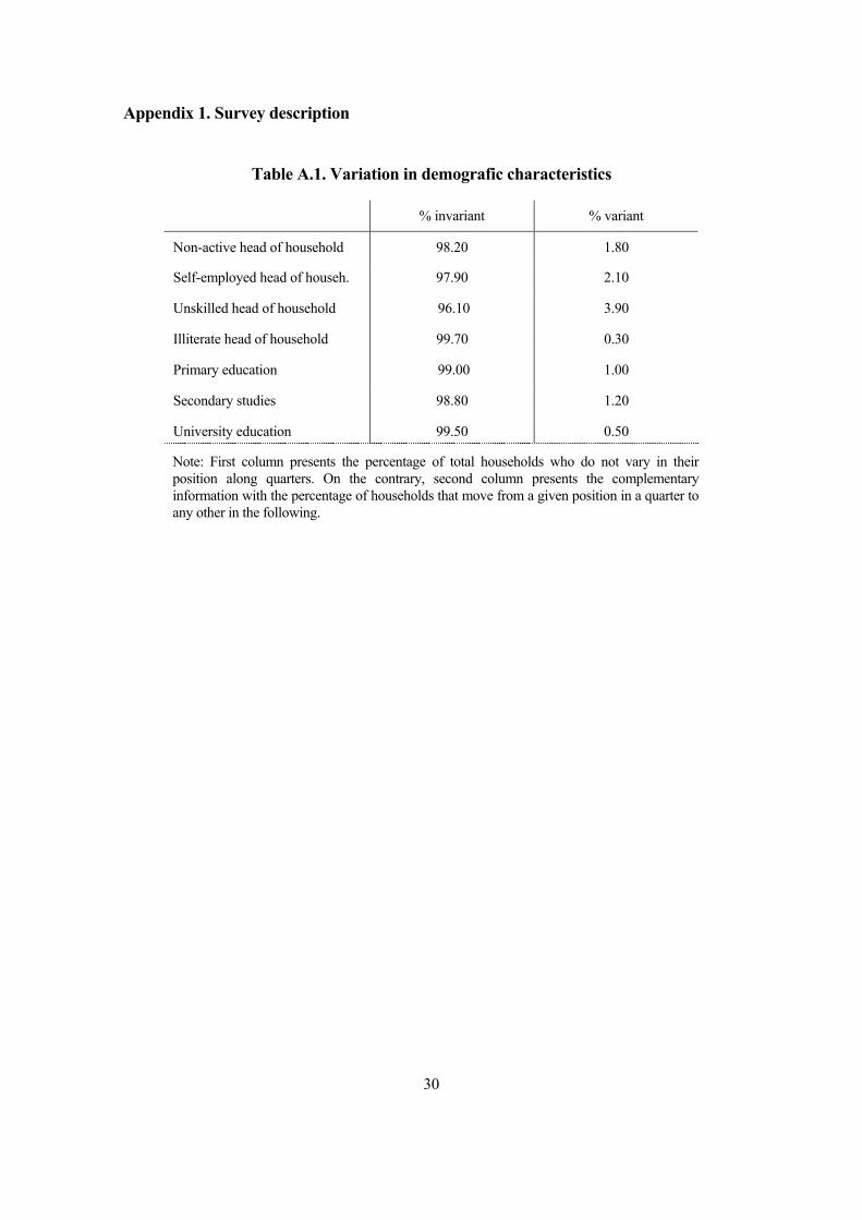
Appendix 1. Survey description

Table A.1. Variation in demografic characteristics

% invariant % variant

Non-active head of household 98.20 1.80

Self-employed head of househ. 97.90 2.10

Unskilled head of household 96.10 3.90

Illiterate head of household 99.70 0.30

Primary education 99.00 1.00

Secondary studies 98.80 1.20

University education 99.50 0.50

Note: First column presents the percentage of total households who do not vary in their position along quarters. On the contrary, second column presents the complementary information with the percentage of households that move from a given position in a quarter to any other in the following.

30

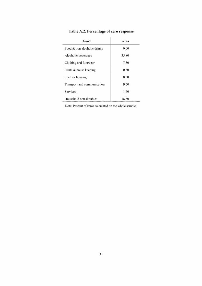
Table A.2. Percentage of zero response

Good zeros

Food & non alcoholic drinks 0.00

Alcoholic beverages 35.80

Clothing and footwear 7.30

Rents & house keeping 0.30

Fuel for housing 0.50

Transport and communication 9.60

Services 1.40

Household non-durables 18.60

Note: Percent of zeros calculated on the whole sample.

31

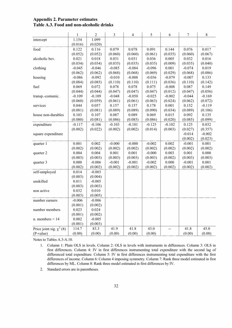
Appendix 2. Parameter estimates Table A.3. Food and non-alcoholic drinks

1 2 3 4 5 6 7 8 intercept 1.154 1.099 (0.016) (0.020) food 0.122 0.116 0.079 0.078 0.091 0.144 0.076 0.017 (0.052) (0.052) (0.060) (0.060) (0.061) (0.035) (0.060) (0.067) alcoholic bev. 0.021 0.018 0.031 0.031 0.036 0.005 0.032 0.016 (0.034) (0.034) (0.035) (0.035) (0.035) (0.009) (0.035) (0.040) clothing -0.045 -0.046 -0.085 -0.084 -0.096 0.001 -0.074 0.019 (0.062) (0.062) (0.068) (0.068) (0.069) (0.029) (0.068) (0.086) housing -0.086 -0.092 -0.010 -0.008 -0.036 -0.079 -0.007 0.133 (0.084) (0.085) (0.110) (0.110) (0.111) (0.036) (0.110) (0.142) fuel 0.069 0.072 0.078 0.078 0.075 -0.008 0.087 0.149 (0.044) (0.044) (0.047) (0.047) (0.047) (0.012) (0.047) (0.056) transp.-comunic. -0.109 -0.109 -0.048 -0.050 -0.025 -0.002 -0.044 -0.169 (0.060) (0.059) (0.061) (0.061) (0.063) (0.024) (0.062) (0.072) services 0.044 0.057 0.157 0.157 0.178 0.001 0.152 -0.119 (0.081) (0.081) (0.089) (0.089) (0.090) (0.034) (0.089) (0.106) house non-durables 0.103 0.107 0.087 0.089 0.069 0.015 0.092 0.135 (0.080) (0.081) (0.086) (0.085) (0.086) (0.020) (0.085) (0.099) expenditure -0.117 -0.106 -0.103 -0.101 -0.125 -0.102 0.125 0.032 (0.002) (0.022) (0.002) (0.002) (0.014) (0.003) (0.027) (0.357) square expenditure -0.014 -0.002 (0.002) (0.023) quarter 1 0.001 0.002 -0.000 -0.000 -0.002 0.002 -0.001 0.001 (0.002) (0.002) (0.002) (0.002) (0.002) (0.002) (0.002) (0.002) quarter 2 0.004 0.004 0.001 0.001 -0.000 0.003 0.001 0.000 (0.003) (0.003) (0.003) (0.003) (0.003) (0.002) (0.003) (0.003) quarter 3 0.000 -0.006 -0.001 -0.001 -0.002 0.000 -0.001 0.001 (0.002) (0.002) (0.002) (0.002) (0.002) (0.002) (0.002) (0.002) self-umployed 0.014 -0.003 (0.003) (0.004) unskilled 0.011 -0.005 (0.003) (0.003) non active 0.032 0.010 (0.003) (0.005) number earners -0.006 -0.006 (0.001) (0.002) number members 0.023 0.024 (0.001) (0.002) n. members < 14 0.002 -0.005 (0.001) (0.003) Price joint sig. χ2 (8) 114.7 83.3 41.9 41.8 43.0 -- 41.8 45.0 (P-value) (0.00) (0.00) (0.00) (0.00) (0.00) (0.00) (0.00) Notes to Tables A.3-A.10.

1. Column 1: Plain OLS in levels. Column 2: OLS in levels with instruments in differences. Column 3: OLS in first differences. Column 4: IV in first differences instrumenting total expenditure with the second lag of differenced total expenditure. Column 5: IV in first differences instrumenting total expenditure with the first differences of income. Column 6: Column 4 imposing symmetry. Column 7: Rank three model estimated in first differences by ML. Column 8: Rank three model estimated in first differences by IV.

2. Standard errors are in parentheses.

32

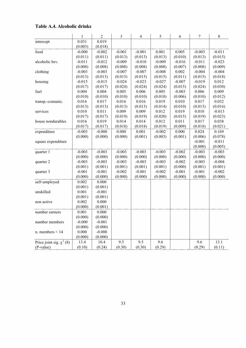
Table A.4. Alcoholic drinks

1 2 3 4 5 6 7 8 intercept 0.031 0.019 (0.003) (0.018) food -0.000 -0.002 -0.001 -0.001 0.001 0.005 -0.003 -0.011 (0.011) (0.011) (0.013) (0.013) (0.013) (0.010) (0.013) (0.015) alcoholic bev. -0.011 -0.012 -0.009 -0.010 -0.009 -0.016 -0.011 -0.023 (0.008) (0.008) (0.008) (0.008) (0.008) (0.007) (0.008) (0.009) clothing -0.003 -0.003 -0.007 -0.007 -0.008 0.002 -0.004 -0.004 (0.013) (0.013) (0.015) (0.015) (0.015) (0.011) (0.015) (0.018) housing -0.015 -0.015 -0.024 -0.023 -0.027 -0.007 -0.019 0.012 (0.017) (0.017) (0.024) (0.024) (0.024) (0.015) (0.024) (0.030) fuel 0.004 0.004 0.005 0.006 0.005 -0.003 0.006 0.009 (0.010) (0.010) (0.010) (0.010) (0.010) (0.006) (0.010) (0.012) transp.-comunic. 0.016 0.017 0.016 0.016 0.019 0.010 0.017 0.032 (0.013) (0.013) (0.013) (0.013) (0.014) (0.010) (0.013) (0.016) services 0.010 0.011 0.009 0.009 0.012 0.019 0.010 -0.013 (0.017) (0.017) (0.019) (0.019) (0.020) (0.015) (0.019) (0.023) house nondurables 0.016 0.019 0.014 0.014 0.012 0.011 0.017 0.038 (0.017) (0.017) (0.018) (0.018) (0.019) (0.009) (0.018) (0.021) expenditure -0.003 -0.000 0.000 0.001 -0.002 0.000 0.024 0.169 (0.000) (0.000) (0.000) (0.001) (0.003) (0.001) (0.006) (0.078) square expenditure -0.001 -0.011 (0.000) (0.005) quarter 1 -0.003 -0.003 -0.003 -0.003 -0.003 -0.002 -0.003 -0.003 (0.000) (0.000) (0.000) (0.000) (0.000) (0.000) (0.000) (0.000) quarter 2 -0.003 -0.003 -0.003 -0.003 -0.003 -0.002 -0.003 -0.004 (0.001) (0.001) (0.001) (0.001) (0.001) (0.000) (0.001) (0.001) quarter 3 -0.001 -0.001 -0.002 -0.001 -0.002 -0.001 -0.001 -0.002 (0.000) (0.000) (0.000) (0.000) (0.000) (0.000) (0.000) (0.000) self-umployed 0.002 0.000 (0.001) (0.001) unskilled 0.001 -0.001 (0.001) (0.001) non active 0.002 0.000 (0.000) (0.001) number earners 0.001 0.000 (0.000) (0.000) number members -0.000 -0.001 (0.000) (0.000) n. members < 14 0.000 -0.000 (0.000) (0.000) Price joint sig. χ2 (8) 13.4 10.4 9.5 9.5 9.6 9.6 13.1 (P-value) (0.10) (0.24) (0.30) (0.30) (0.29) (0.29) (0.11)

33

Table A.5. Clothing and footwear

1 2 3 4 5 6 7 8 intercept -0.226 -0.400 (0.014) (0.078) Food -0.016 -0.024 -0.088 -0.086 -0.087 0.001 -0.091 -0.096 (0.049) (0.049) (0.059) (0.059) (0.060) (0.029) (0.059) (0.068) alcoholic bev. -0.030 -0.031 -0.042 -0.041 -0.043 0.002 -0.042 -0.018 (0.034) (0.034) (0.035) (0.035) (0.035) (0.011) (0.035) (0.042) clothing 0.102 0.099 0.105 0.104 0.108 -0.034 0.113 0.002 (0.056) (0.057) (0.066) (0.066) (0.066) (0.045) (0.066) (0.084) housing -0.021 -0.015 0.267 0.265 0.267 -0.054 0.281 0.322 (0.073) (0.073) (0.108) (0.108) (0.109) (0.040) (0.108) (0.143) Fuel 0.042 0.042 0.033 0.032 0.034 -0.044 0.046 -0.013 (0.043) (0.043) (0.046) (0.046) (0.046) (0.014) (0.046) (0.056) transp.-comunic. 0.047 0.032 0.008 0.011 0.006 0.011 0.019 0.109 (0.058) (0.057) (0.060) (0.060) (0.062) (0.029) (0.060) (0.072) services -0.014 -0.019 -0.074 -0.072 -0.078 0.086 -0.089 0.024 (0.079) (0.079) (0.087) (0.087) (0.088) (0.040) (0.087) (0.107) house nondurables 0.187 0.212 0.213 0.211 0.214 -0.012 0.219 0.211 (0.077) (0.077) (0.083) (0.083) (0.084) (0.020) (0.083) (0.098) expenditure 0.045 0.069 0.076 0.073 0.079 0.075 0.376 -0.116 (0.001) (0.002) (0.002) (0.002) (0.013) (0.003) (0.027) (0.361) square expenditure -0.019 0.012 (0.002) (0.023) quarter 1 -0.001 -0.001 0.001 0.001 0.001 0.003 0.000 -0.002 (0.002) (0.002) (0.002) (0.002) (0.002) (0.002) (0.002) (0.002) quarter 2 -0.006 -0.007 -0.011 -0.007 -0.007 -0.004 -0.008 -0.010 (0.002) (0.003) (0.003) (0.003) (0.003) (0.002) (0.003) (0.003) quarter 3 -0.017 -0.018 -0.016 -0.016 -0.016 -0.017 -0.016 -0.019 (0.002) (0.002) (0.002) (0.002) (0.002) (0.002) (0.002) (0.002) self-umployed 0.005 0.008 (0.002) (0.004) unskilled 0.010 0.003 (0.002) (0.003) non active 0.001 -0.003 (0.002) (0.005) number earners 0.006 0.008 (0.001) (0.002) number members 0.001 -0.002 (0.001) (0.002) n. members < 14 -0.006 -0.001 (0.001) (0.002) Price joint sig. χ2 (8) 33.4 25.3 11.8 11.6 11.7 12.6 24.1 (P-value) (0.00) (0.00) (0.16) (0.17) (0.17) (0.13) (0.00)

34

Table A.6. Housing expenses

1 2 3 4 5 6 7 8 intercept 0.476 0.564 (0.016) (0.018) food -0.080 -0.074 -0.073 -0.073 -0.101 -0.079 -0.046 -0.065 (0.047) (0.047) (0.051) (0.051) (0.053) (0.036) (0.051) (0.052) alcoholic bev. 0.052 0.056 0.064 0.064 0.055 -0.007 0.067 0.085 (0.030) (0.030) (0.030) (0.030) (0.031) (0.015) (0.030) (0.059) clothing -0.086 -0.089 -0.101 -0.101 -0.084 -0.054 -0.107 -0.070 (0.058) (0.058) (0.061) (0.061) (0.063) (0.040) (0.060) (0.036) housing 0.010 0.007 -0.146 -0.147 -0.094 -0.014 -0.188 -0.207 (0.082) (0.083) (0.098) (0.098) (0.101) (0.076) (0.097) (0.079) fuel -0.062 -0.062 -0.050 -0.050 -0.044 -0.070 -0.058 -0.006 (0.039) (0.039) (0.041) (0.041) (0.042) (0.019) (0.041) (0.132) transp.-comunic. -0.024 -0.020 -0.035 -0.035 -0.076 0.001 -0.041 -0.127 (0.054) (0.054) (0.055) (0.055) (0.057) (0.038) (0.054) (0.051) services 0.024 0.017 0.008 0.009 -0.030 0.060 0.026 -0.074 (0.074) (0.075) (0.079) (0.079) (0.081) (0.054) (0.078) (0.067) house nondurables -0.168 -0.179 -0.084 -0.085 -0.045 0.007 -0.116 -0.123 (0.073) (0.073) (0.076) (0.076) (0.078) (0.031) (0.075) (0.097) expenditure -0.029 -0.044 -0.055 -0.055 -0.014 -0.054 -0.710 0.096 (0.001) (0.019) (0.002) (0.002) (0.012) (0.004) (0.023) (0.316) square expenditure 0.041 -0.009 (0.001) (0.020) quarter 1 -0.007 -0.003 -0.008 -0.008 -0.005 -0.009 -0.007 -0.007 (0.002) (0.002) (0.002) (0.002) (0.002) (0.001) (0.002) (0.002) quarter 2 -0.008 -0.004 -0.009 -0.009 -0.006 -0.010 -0.007 -0.007 (0.002) (0.003) (0.002) (0.002) (0.003) (0.002) (0.002) (0.003) quarter 3 0.000 0.004 -0.001 -0.001 0.002 -0.000 -0.000 -0.001 (0.002) (0.002) (0.002) (0.002) (0.002) (0.001) (0.002) (0.002) self-umployed -0.008 -0.002 (0.003) (0.004) unskilled -0.011 -0.002 (0.002) (0.003) non active -0.002 0.009 (0.003) (0.004) number earners -0.006 -0.005 (0.001) (0.002) number members -0.011 -0.014 (0.001) (0.003) n. members < 14 -0.002 -0.003 (0.001) (0.003) Price joint sig. χ2 (8) 53.9 33.5 18.3 18.3 17.9 20.1 22.8 (P-value) (0.00) (0.00) (0.02) (0.02) (0.02) (0.01) (0.00)

35

Table A.7. Fuel for housing

1 2 3 4 5 6 7 8 intercept 0.202 0.234 (0.004) (0.023) Food -0.025 -0.024 0.000 0.000 0.004 -0.008 0.002 -0.006 (0.014) (0.014) (0.017 (0.017) (0.017) (0.012) (0.017) (0.020) alcoholic bev. -0.028 -0.028 -0.019 -0.020 -0.018 -0.003 -0.020 -0.024 (0.009) (0.009) (0.010 (0.010) (0.010) (0.006) (0.010) (0.012) Clothing -0.018 -0.018 -0.040 -0.040 -0.043 -0.044 -0.041 -0.014 (0.016) (0.016) (0.018 (0.018) (0.018) (0.014) (0.018) (0.024) Housing -0.030 -0.029 -0.086 -0.086 -0.092 -0.070 -0.088 -0.054 (0.021) (0.021) (0.029 (0.023) (0.030) (0.019) (0.029) (0.041) fuel 0.013 0.012 0.001 0.001 -0.000 0.003 0.001 0.015 (0.012) (0.012) (0.013 (0.013) (0.013) (0.010) (0.013) (0.016) transp.-comunic. 0.034 0.036 0.062 0.061 0.067 0.048 0.063 0.036 (0.016) (0.016) (0.017 (0.017) (0.017) (0.014) (0.017) (0.021) services 0.053 0.053 0.111 0.111 0.117 0.078 0.113 0.071 (0.022) (0.022) (0.024 (0.024) (0.024) (0.020) (0.024) (0.031) house nondurables 0.038 0.034 0.007 0.008 0.003 0.003 0.006 -0.001 (0.021) (0.021) (0.023 (0.023) (0.023) (0.012) (0.023) (0.028) expenditure -0.021 -0.024 -0.026 -0.026 -0.030 -0.026 -0.108 0.048 (0.000) (0.003) (0.001 (0.001) (0.004) (0.001) (0.007) (0.103) square expenditure 0.005 -0.005 (0.000) (0.007) quarter 1 0.005 0.005 0.004 0.004 0.004 0.004 0.004 0.005 (0.000) (0.001) (0.001) (0.001) (0.001) (0.001) (0.001) (0.001) quarter 2 0.002 0.002 0.002 0.002 0.001 0.002 0.002 0.002 (0.001) (0.001) (0.001) (0.001) (0.001) (0.001) (0.001) (0.001) quarter 3 -0.002 -0.003 -0.003 -0.003 -0.003 -0.003 -0.003 -0.003 (0.000) (0.001) (0.001) (0.001) (0.001) (0.000) (0.001) (0.002) self-umployed -0.000 -0.001 (0.001) (0.001) unskilled -0.002 0.000 (0.001) (0.001) non active 0.001 0.001 (0.001) (0.001) number earners 0.000 -0.000 (0.000) (0.000) number members 0.000 -0.000 (0.000) (0.001) n. members < 14 0.000 0.000 (0.000) (0.001) Price joint sig. χ2 (8) 71.7 65.5 111.4 110.9 88.4 113.9 34.7 (P-value) (0.00) (0.00) (0.00) (0.00) (0.00) (0.00) (0.00)

36

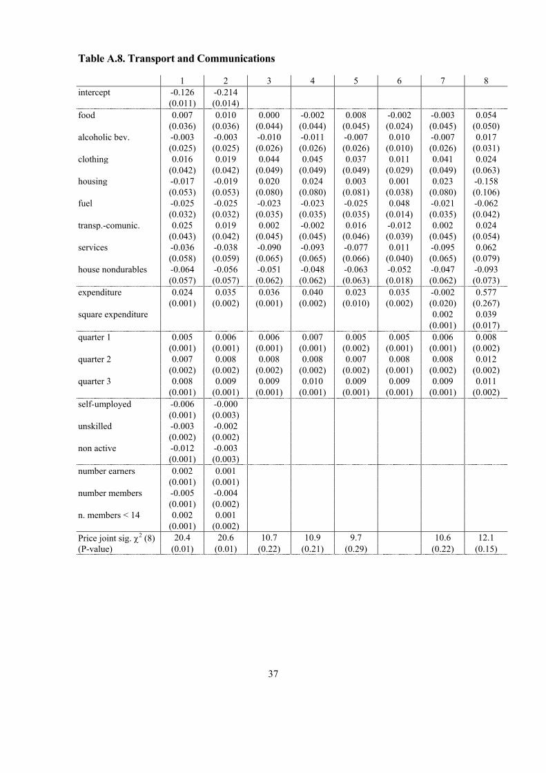
Table A.8. Transport and Communications

1 2 3 4 5 6 7 8 intercept -0.126 -0.214 (0.011) (0.014) food 0.007 0.010 0.000 -0.002 0.008 -0.002 -0.003 0.054 (0.036) (0.036) (0.044) (0.044) (0.045) (0.024) (0.045) (0.050) alcoholic bev. -0.003 -0.003 -0.010 -0.011 -0.007 0.010 -0.007 0.017 (0.025) (0.025) (0.026) (0.026) (0.026) (0.010) (0.026) (0.031) clothing 0.016 0.019 0.044 0.045 0.037 0.011 0.041 0.024 (0.042) (0.042) (0.049) (0.049) (0.049) (0.029) (0.049) (0.063) housing -0.017 -0.019 0.020 0.024 0.003 0.001 0.023 -0.158 (0.053) (0.053) (0.080) (0.080) (0.081) (0.038) (0.080) (0.106) fuel -0.025 -0.025 -0.023 -0.023 -0.025 0.048 -0.021 -0.062 (0.032) (0.032) (0.035) (0.035) (0.035) (0.014) (0.035) (0.042) transp.-comunic. 0.025 0.019 0.002 -0.002 0.016 -0.012 0.002 0.024 (0.043) (0.042) (0.045) (0.045) (0.046) (0.039) (0.045) (0.054) services -0.036 -0.038 -0.090 -0.093 -0.077 0.011 -0.095 0.062 (0.058) (0.059) (0.065) (0.065) (0.066) (0.040) (0.065) (0.079) house nondurables -0.064 -0.056 -0.051 -0.048 -0.063 -0.052 -0.047 -0.093 (0.057) (0.057) (0.062) (0.062) (0.063) (0.018) (0.062) (0.073) expenditure 0.024 0.035 0.036 0.040 0.023 0.035 -0.002 0.577 (0.001) (0.002) (0.001) (0.002) (0.010) (0.002) (0.020) (0.267) square expenditure 0.002 0.039 (0.001) (0.017) quarter 1 0.005 0.006 0.006 0.007 0.005 0.005 0.006 0.008 (0.001) (0.001) (0.001) (0.001) (0.002) (0.001) (0.001) (0.002) quarter 2 0.007 0.008 0.008 0.008 0.007 0.008 0.008 0.012 (0.002) (0.002) (0.002) (0.002) (0.002) (0.001) (0.002) (0.002) quarter 3 0.008 0.009 0.009 0.010 0.009 0.009 0.009 0.011 (0.001) (0.001) (0.001) (0.001) (0.001) (0.001) (0.001) (0.002) self-umployed -0.006 -0.000 (0.001) (0.003) unskilled -0.003 -0.002 (0.002) (0.002) non active -0.012 -0.003 (0.001) (0.003) number earners 0.002 0.001 (0.001) (0.001) number members -0.005 -0.004 (0.001) (0.002) n. members < 14 0.002 0.001 (0.001) (0.002) Price joint sig. χ2 (8) 20.4 20.6 10.7 10.9 9.7 10.6 12.1 (P-value) (0.01) (0.01) (0.22) (0.21) (0.29) (0.22) (0.15)

37

Table A.9. Services

1 2 3 4 5 6 7 8 intercept -0.211 -0.127 (0.016) (0.020) food -0.020 -0.012 0.075 0.076 0.043 0.001 0.071 0.084 (0.051) (0.051) (0.059) (0.060) (0.060) (0.034) (0.060) (0.066) alcoholic bev. 0.024 0.025 0.013 0.013 0.001 0.019 0.012 -0.020 (0.035) (0.035) (0.035) (0.035) (0.035) (0.015) (0.035) (0.040) clothing -0.001 0.006 0.037 0.036 0.062 0.086 0.042 0.006 (0.061) (0.061) (0.068) (0.068) (0.069) (0.040) (0.068) (0.085) housing 0.085 0.088 -0.087 -0.089 -0.023 0.060 -0.076 -0.048 (0.082) (0.083) (0.110) (0.110) (0.111) (0.054) (0.110) (0.141) fuel -0.015 -0.019 -0.061 -0.062 -0.055 0.078 -0.056 -0.076 (0.044) (0.044) (0.047) (0.047) (0.047) (0.020) (0.047) (0.056) transp.-comunic. 0.065 0.069 0.067 0.069 0.009 0.011 0.077 0.187 (0.059) (0.060) (0.061) (0.061) (0.063) (0.040) (0.061) (0.072) services -0.034 -0.046 -0.005 -0.004 -0.054 -0.045 -0.005 0.077 (0.081) (0.081) (0.088) (0.088) (0.090) (0.075) (0.089) (0.105) house nondurables -0.073 -0.082 -0.153 -0.155 -0.108 -0.021 -0.148 -0.071 (0.080) (0.081) (0.085) (0.085) (0.086) (0.027) (0.085) (0.098) expenditure 0.045 0.032 0.040 0.038 0.094 0.041 0.260 0.605 (0.002) (0.002) (0.002) (0.002) (0.013) (0.003) (0.027) (0.355) square expenditure -0.014 -0.036 (0.002) (0.022) quarter 1 -0.001 -0.002 0.001 0.000 0.005 -0.001 0.000 -0.002 (0.002) (0.002) (0.002) (0.002) (0.002) (0.002) (0.002) (0.002) quarter 2 0.002 0.001 0.006 0.006 0.009 0.004 0.005 0.003 (0.003) (0.003) (0.003) (0.003) (0.003) (0.002) (0.003) (0.003) quarter 3 0.014 0.013 0.015 0.015 0.019 0.015 0.015 0.014 (0.002) (0.002) (0.002) (0.002) (0.002) (0.002) (0.002) (0.002) self-umployed -0.006 0.005 (0.003) (0.004) unskilled -0.003 0.005 (0.002) (0.003) non active -0.033 -0.008 (0.002) (0.005) number earners 0.006 0.003 (0.001) (0.002) number members -0.001 -0.001 (0.001) (0.003) n. members < 14 0.008 0.011 (0.001) (0.003) Price joint sig. χ2 (8) 65.5 57.7 18.7 18.8 10.1 18.4 23.3 (P-value) (0.00) (0.00) (0.02) (0.02) (0.26) (0.02) (0.00)

38

Table A.10. Household non-durables

1 2 3 4 5 6 7 8 intercept 0.025 0.046 (0.006) (0.031) food 0.028 0.026 0.019 0.019 0.025 0.015 0.017 0.009 (0.018) (0.018) (0.021) (0.021) (0.021) (0.020) (0.021) (0.023) alcoholic bev. 0.006 0.005 0.006 0.007 0.009 0.011 0.006 0.003 (0.012) (0.012) (0.012) (0.012) (0.012) (0.009) (0.012) (0.014) clothing -0.025 -0.024 -0.040 -0.040 -0.044 0.007 -0.039 -0.040 (0.022) (0.022) (0.024) (0.024) (0.024) (0.031) (0.024) (0.030) housing -0.022 -0.018 -0.012 -0.011 -0.023 0.007 -0.009 0.010 (0.029) (0.029) (0.039) (0.039) (0.040) (0.031) (0.039) (0.050) fuel -0.009 -0.009 -0.001 -0.001 -0.002 0.003 0.000 0.004 (0.015) (0.015) (0.017) (0.017) (0.017) (0.012) (0.017) (0.019) transp.-comunic. -0.051 -0.047 -0.054 -0.054 -0.043 -0.052 -0.052 -0.074 (0.021) (0.021) (0.022) (0.022) (0.022) (0.018) (0.022) (0.025) services 0.025 0.023 0.024 0.023 0.032 -0.021 0.021 0.020 (0.028) (0.029) (0.031) (0.031) (0.032) (0.027) (0.031) (0.037) house non-durables -0.035 -0.039 -0.036 -0.036 -0.045 -0.033 -0.032 -0.041 (0.028) (0.028) (0.030) (0.030) (0.030) (0.027) (0.030) (0.034) expenditure -0.001 -0.172 -0.002 -0.001 -0.011 -0.002 0.072 0.135 (0.001) (0.001) (0.001) (0.001) (0.005) (0.001) (0.009) (0.124) square expenditure -0.005 -0.009 (0.001) (0.008) quarter 1 0.002 0.002 0.002 0.002 0.001 0.002 0.001 0.002 (0.001) (0.001) (0.001) (0.001) (0.001) (0.001) (0.001) (0.001) quarter 2 0.003 0.003 0.002 0.002 0.002 0.003 0.002 0.002 (0.001) (0.001) (0.001) (0.001) (0.001) (0.001) (0.001) (0.001) quarter 3 0.002 0.002 0.001 0.001 0.001 0.002 0.001 0.002 (0.001) (0.001) (0.001) (0.001) (0.001) (0.001) (0.001) (0.001) self-umployed -0.001 -0.002 (0.001) (0.002) unskilled -0.000 -0.001 (0.001) (0.001) non active 0.004 -0.000 (0.001) (0.002) number earners 0.001 -0.001 (0.000) (0.001) number members 0.001 -0.001 (0.000) (0.001) n. members < 14 -0.004 -0.001 (0.000) (0.001) Price joint sig. χ2 (8) 34.9 23.6 17.6 17.6 12.6 17.4 22.6 (P-value) (0.00) (0.00) (0.02) (0.02) (0.13) (0.03) (0.00)

39