Demand Side Management opportunities for a typical South

Demand Side Management opportunities for a

typical South African cement plant

Raine Tamsin Lidbetter

22647554

Dissertation submitted in fulfilment of the requirements for the degree

Magister in Mechanical Engineering at the Potchefstroom campus of

the North-West University

Supervisor: Professor Leon Liebenberg

November 2010

i

ABSTRACT

The South African electrical system is under threat of supply shortage. This is because, in the last

decade, the maximum electrical demand has been encroaching on the net maximum capacity and the

reserve storage margin has become smaller. Eskom, the country’s electricity utility, has implemented a

demand side management (DSM) programme in an attempt to alleviate the threat. Investigations into

demand side reductions have been encouraged by the utility in sectors with high electricity

consumption, such as the cement industry. As part of the non-metallic minerals sector, it is responsible

for 5% of the electrical consumption for the mining and industrial division of the country. It has also

been estimated that by 2020 the sector will be ranked as fifth for energy savings potential. Therefore,

there may be opportunities to reduce the power demand of cement plants thus assisting Eskom in

reducing the country’s electrical consumption. This can be done by implementing DSM programmes,

such as energy efficiency and load management. This dissertation investigates the global opportunities

for energy efficiency in cement plants and determines their feasibility for the South African cement

industry. It also investigates the potential of a load-shifting scheme to reduce evening peak loads and

save electrical costs. To evaluate DSM potential for an undisclosed South African cement plant, historical

data on electrical consumption was used in a simulation programme which the author wrote. This was

done to determine a possible load-shifting scheme which could be implemented to save costs and

reduce peak-period demand. A pilot study was performed to evaluate how shifting the load of raw and

cement mills would affect the production and electrical costs of the plant. Results showed that, although

in theory there is good opportunity for cost savings, it is highly dependent on the reliability of the mills

and the change in production demand. Therefore, load-shifting schemes have to be highly adaptable on

a daily basis to shift load when possible.

ii

PREFACE AND ACKNOWLEDGEMENTS

It is my hope that this dissertation motivates energy efficiency in the South African and global cement

industry. Whoever wishes to increase their knowledge, continue research in the topic or implement the

strategies, I wish you the best of success.

I would firstly like to thank my mom and dad, Essie and Dave, who have encouraged me and stood by

me my entire life. Your support has made me believe I can achieve anything I put my mind and heart

into.

A special thanks to Prof Leon Liebenberg for his indispensable guidance and advice throughout the

study. You have spent many, many hours helping me and proof reading the document, for which I am

extremely grateful.

Thank you to Prof Eddie Mathews and Dr Marius Kleingeld for giving me the opportunity to do my

masters. I have thoroughly enjoyed working on this dissertation and project.

Thank you to Mr Douglas Velleman for proof reading and helping with the technical side of the

document.

Thanks to the cement plant engineers who provided me with the data and performed the pilot study,

without which the study could not have been conducted.

Thank you to Dave Taylor for affording me the opportunity to pursue my master’s studies.

Thanks to my sister, brothers and friends for being there. Your love and support has kept me sane in

times of stress and pressure.

And finally, I would like to thank God for blessing me with the opportunities, family, friends and

colleagues I have been given. It is only through His love that I am able to be who I am.

iii

TABLE OF CONTENTS

Abstract i

Preface and Acknowledgements ii

Table of contents iii

List of figures vi

List of tables viii

List of equations ix

List of symbols ix

List of abbreviations x

Nomenclature xi

Chapter 1 Introduction to study Page

1.1 Background: Electrical energy situation 1

Global electricity usage trends 2

South African electricity situation 3

Eskom’s new build and recovery programmes 4

Demand Side Management (DSM) 5

DSM motivation 7

DSM initiatives in the residential sector 8

Energy service company and project scopes 9

DSM initiatives in industrial, commercial and mining sectors 10

1.2 Motivation for the study 11

South African energy saving case study 11

Determining the value of a DSM initiative investigation 12

Cement plant energy consumption 14

Cement plant DSM opportunity overview 14

1.3 Objectives of the study 16

1.4 Scope of the study 16

1.5 Layout of dissertation 16

1.6 References 17

Chapter 2 Energy efficiency and load-shifting opportunities in the cement industry

2.1 South African cement production plants 19

Portland cement 20

Dry process cement production 20

Obtaining raw materials 20

Raw mill and silo 22

Preheating 23

Kiln, cooler and clinker silo 23

iv

Cement/finishing mill 25

Cement silos and packaging 25

2.2 Electrical consumption by department 25

2.3 Potential for energy efficiency 26

Overall potential classification 27

Energy efficiency opportunities in the cement industry 27

Raw material process 29

Clinker burning process 30

Finishing process 30

Plant Wide Measures 31

2.4 Priorities and barriers in DSM initiatives 31

Influential factors 33

2.5 Evaluating validity of opportunities 34

2.6 Scope of ESCO contracts for the cement industry 35

2.7 Conclusion 37

2.8 References 37

Chapter 3 Evaluation and simulation of a typical South African cement plant

3.1 The cement plant under investigation 41

Plant information 42

Energy efficiency opportunities 42

Load-shifting opportunities 44

3.2 Baselines 46

3.3 Load-shifting functions 49

Silo simulation 50

Raw meal silo 51

Clinker silo simulation 55

Silo simulation results 57

3.4 Optimised baseline 57

3.5 Savings potential 61

Theoretical results 65

3.6 Pilot study 66

3.7 Conclusion 66

3.8 References 66

Chapter 4 Pilot study

4.1 Pilot study 68

Aim of the pilot study 69

Assumptions and contingencies 69

Method 69

Required information 70

v

4.2 Power consumption and baselines of the mills during the pilot study 70

Cement mill 1 71

Cement mill 2 72

Raw mill 4 73

Raw mill 3 75

4.3 Performance of the silo simulation 76

4.4 Change in cost 77

4.5 Change in peak period consumption 82

4.6 Additional pilot study 82

4.7 Conclusion 84

Chapter 5 Conclusion

5.1 Revision of the goal 86

5.2 Energy efficiency options for the typical South African cement industry 87

5.3 Load-shifting opportunities for the typical South African cement plant 87

5.4 Recommendations 89

5.5 Final Conclusion 90

List of References 92

Appendix

A Cement plant questionnaire 97

B Data collection and summary 102

Stoppage hours 102

Flow rates 104

C Simulation software 105

Raw meal silo 105

Clinker silo 107

Baseline 110

D Probability of a positive silo change 112

E Recommended simulation software 113

vi

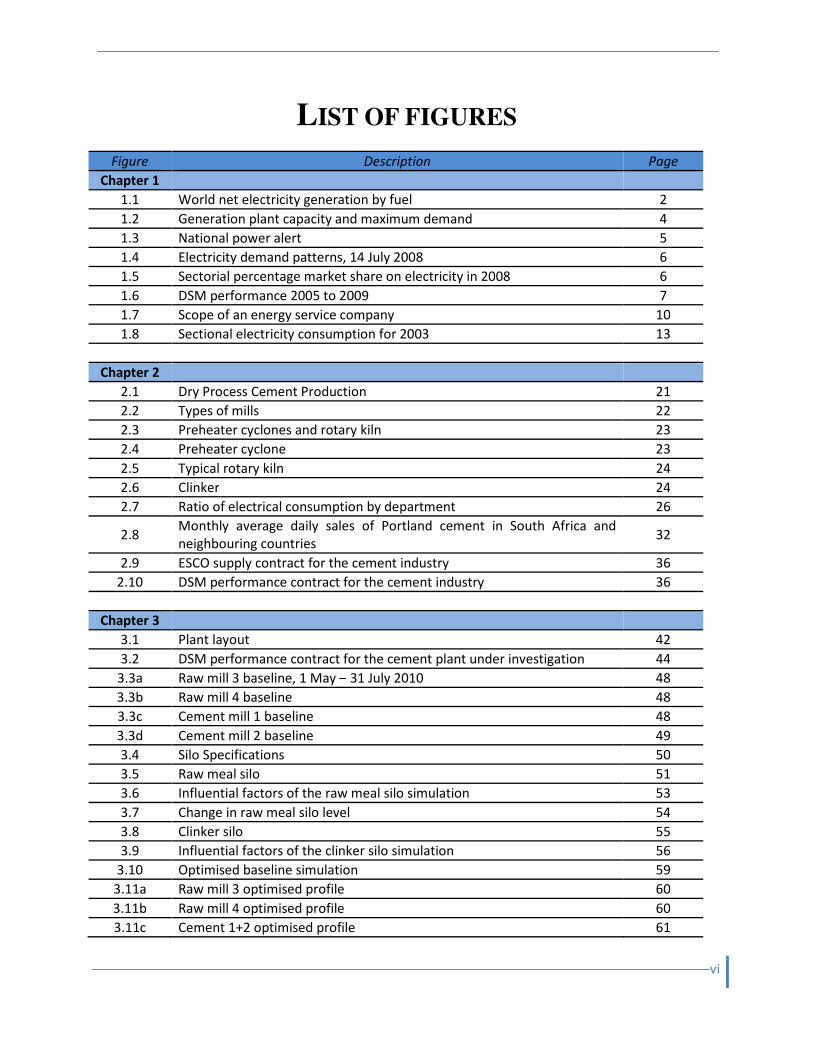
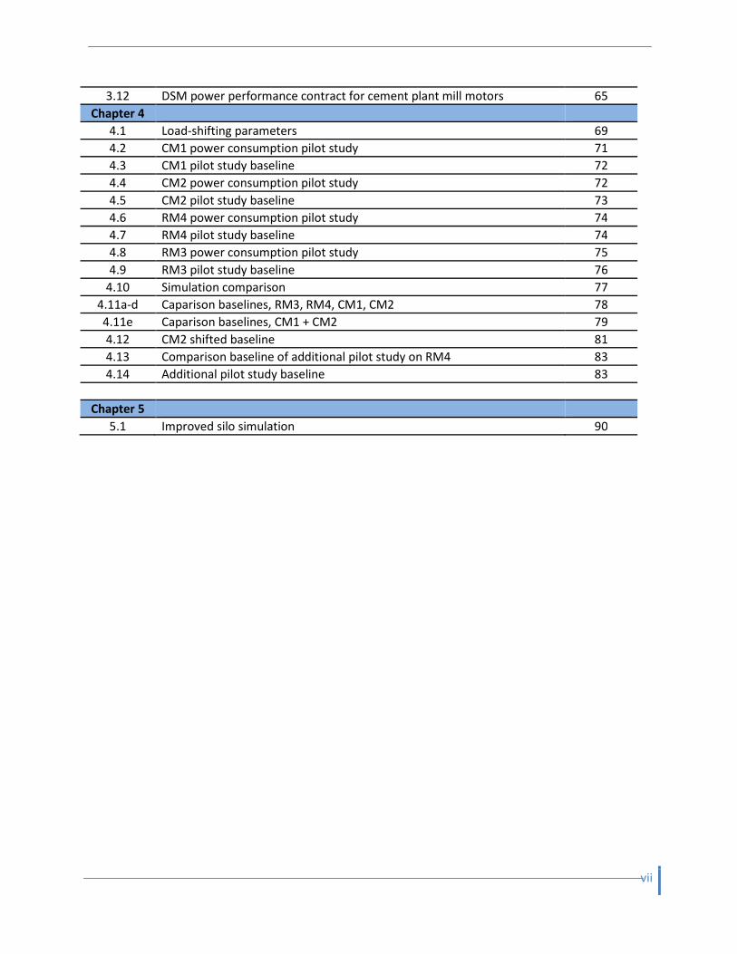
LIST OF FIGURES

Figure Description Page

Chapter 1

1.1 World net electricity generation by fuel 2

1.2 Generation plant capacity and maximum demand 4

1.3 National power alert 5

1.4 Electricity demand patterns, 14 July 2008 6

1.5 Sectorial percentage market share on electricity in 2008 6

1.6 DSM performance 2005 to 2009 7

1.7 Scope of an energy service company 10

1.8 Sectional electricity consumption for 2003 13

Chapter 2

2.1 Dry Process Cement Production 21

2.2 Types of mills 22

2.3 Preheater cyclones and rotary kiln 23

2.4 Preheater cyclone 23

2.5 Typical rotary kiln 24

2.6 Clinker 24

2.7 Ratio of electrical consumption by department 26

2.8 Monthly average daily sales of Portland cement in South Africa and

neighbouring countries 32

2.9 ESCO supply contract for the cement industry 36

2.10 DSM performance contract for the cement industry 36

Chapter 3

3.1 Plant layout 42

3.2 DSM performance contract for the cement plant under investigation 44

3.3a Raw mill 3 baseline, 1 May – 31 July 2010 48

3.3b Raw mill 4 baseline 48

3.3c Cement mill 1 baseline 48

3.3d Cement mill 2 baseline 49

3.4 Silo Specifications 50

3.5 Raw meal silo 51

3.6 Influential factors of the raw meal silo simulation 53

3.7 Change in raw meal silo level 54

3.8 Clinker silo 55

3.9 Influential factors of the clinker silo simulation 56

3.10 Optimised baseline simulation 59

3.11a Raw mill 3 optimised profile 60

3.11b Raw mill 4 optimised profile 60

3.11c Cement 1+2 optimised profile 61

vii

3.12 DSM power performance contract for cement plant mill motors 65

Chapter 4

4.1 Load-shifting parameters 69

4.2 CM1 power consumption pilot study 71

4.3 CM1 pilot study baseline 72

4.4 CM2 power consumption pilot study 72

4.5 CM2 pilot study baseline 73

4.6 RM4 power consumption pilot study 74

4.7 RM4 pilot study baseline 74

4.8 RM3 power consumption pilot study 75

4.9 RM3 pilot study baseline 76

4.10 Simulation comparison 77

4.11a-d Caparison baselines, RM3, RM4, CM1, CM2 78

4.11e Caparison baselines, CM1 + CM2 79

4.12 CM2 shifted baseline 81

4.13 Comparison baseline of additional pilot study on RM4 83

4.14 Additional pilot study baseline 83

Chapter 5

5.1 Improved silo simulation 90

viii

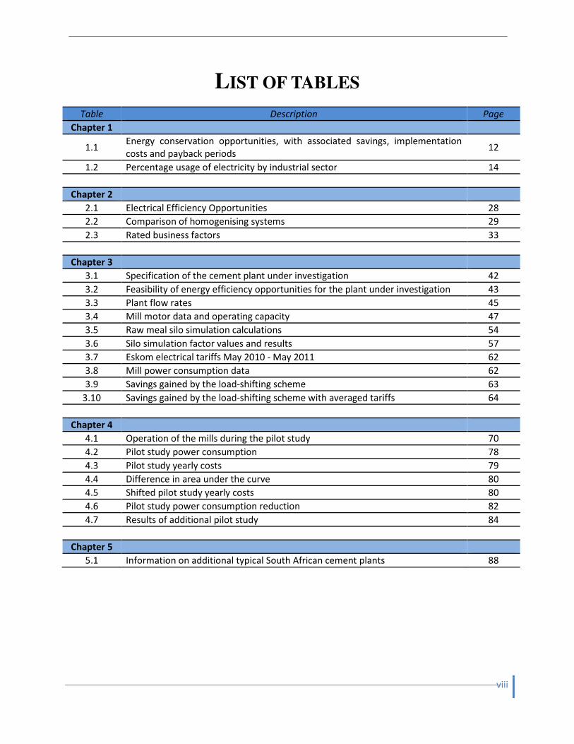
LIST OF TABLES

Table Description Page

Chapter 1

1.1 Energy conservation opportunities, with associated savings, implementation

costs and payback periods 12

1.2 Percentage usage of electricity by industrial sector 14

Chapter 2

2.1 Electrical Efficiency Opportunities 28

2.2 Comparison of homogenising systems 29

2.3 Rated business factors 33

Chapter 3

3.1 Specification of the cement plant under investigation 42

3.2 Feasibility of energy efficiency opportunities for the plant under investigation 43

3.3 Plant flow rates 45

3.4 Mill motor data and operating capacity 47

3.5 Raw meal silo simulation calculations 54

3.6 Silo simulation factor values and results 57

3.7 Eskom electrical tariffs May 2010 - May 2011 62

3.8 Mill power consumption data 62

3.9 Savings gained by the load-shifting scheme 63

3.10 Savings gained by the load-shifting scheme with averaged tariffs 64

Chapter 4

4.1 Operation of the mills during the pilot study 70

4.2 Pilot study power consumption 78

4.3 Pilot study yearly costs 79

4.4 Difference in area under the curve 80

4.5 Shifted pilot study yearly costs 80

4.6 Pilot study power consumption reduction 82

4.7 Results of additional pilot study 84

Chapter 5

5.1 Information on additional typical South African cement plants 88

ix

LIST OF EQUATIONS

Equation Description Page

1 �� – �� 50

2 �� 24 – �� – �� – �� 52

3 � �1 � �2 � �3 64

4 �1

�1

� 64

5

�2 �2

� 64

6 � �1 1 � �2 2 � !1 " �1 " �2# 3 64

7 � � $ ∆� 64

LIST OF SYMBOLS

Symbol Description Unit

Q Energy consumption kWh

S Energy consumption ratio

W Tariff weighted average R

w Tariff R

C Cost savings R

Subscript

1 Peak period

2 Off-peak

3 Standard

x

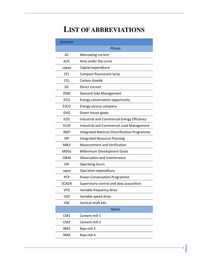
LIST OF ABBREVIATIONS

Acronym

Phrase

AC Alternating current

AUC Area under the curve

capex Capital expenditure

CFL Compact fluorescent lamp

CO2 Carbon dioxide

DC Direct current

DSM Demand Side Management

ECO Energy conservation opportunity

ESCO Energy service company

GHG Green house gases

ICEE Industrial and Commercial Energy Efficiency

ICLM Industrial and Commercial Load Management

INEP Integrated National Electrification Programme

IRP Integrated Resource Planning

M&V Measurement and Verification

MDGs Millennium Development Goals

O&M Observation and maintenance

OH Operating hours

opex Operation expenditure

PCP Power Conservation Programme

SCADA Supervisory control and data acquisition

VFD Variable frequency drive

VSD Variable speed drive

VSK Vertical shaft kiln

Name

CM1 Cement mill 1

CM2 Cement mill 2

RM3 Raw mill 3

RM4 Raw mill 4

xi

GLOSSARY

Object Description

Cement Cement is a bonding agent which hardens and binds building materials

Chalk A soft, white, powdery limestone consisting of fossil shells

Clay A natural earthy material that is plastic when wet

Concrete A stone-like material used for various structural purposes, made by mixing

cement and various aggregate

ESCO contract scope The areas of focus during an ECSO investigation into DSM opportunities

Fly ash Fine particles of ash of a solid fuel carried out of the flue of a furnace with

the waste gases produced during combustion

Grout A fine plaster used as a finishing coat

Mortar Used as a bonding agent between bricks and stones

Prehomogenising pile A stock pile where materials are mixed to an even consistency

Shale A dark fine-grained rock formed by compression of successive layers of

clay-rich sediment

Slag A mixture of shale, clay, coal dust, and other mineral waste produced

during coal mining

Stucco Used in decorative mouldings on buildings

1 Chapter 1

Chapter 1

Introduction to Study

1.1. Background: Electrical energy situation

It is said that the prime mover for economic growth and development of a country is its energy

consumption (Alam, et al., 1991). Regarding this, the total energy used per capita is a measure for

the standard of living or quality of life achieved in all communities (Sheffield, 1998). It has therefore

been encouraged in modern society to consume available energy without constraint to achieve the

highest quality of life.

As one looks at the global usage of non-renewable energy and the implications on the ecology, it is

evident that present energy utilisation rates cannot be sustained without future consequences. This

chapter investigates opportunities of energy saving programmes in South African industry to

participate in lowering global energy consumption.

2 Chapter 1

Global electricity usage trends

In terms of end use, electricity is the most efficient form of energy (Kim and Starr, 2000). It provides

a means in achieving many of the basic needs of humans. With the natural progression of technology

and the instinct to reproduce, people are forced to produce and consume an increasing amount of

electricity to meet these needs.

The world population has increased considerably since the discovery of electricity in the 18th

century. With an increase from 700 million in 1750 to 6.8 billion in 2009, and a projected estimate of

9.4 billion people by 2050, it is clear that humans are fast reaching alarming numbers (Matt, 2010).

This growing population along with the improvement of information technology, biotechnology,

advanced manufacturing and other technologies will result in growth of global electrical demand

(Kim and Starr, 2000). If the demand is to be supplied by renewable sources, it would allow for a

sustainable future. Currently, however, it is projected that only 10% of required electricity by 2020

will be generated by renewable sources (Bozon et al., 2007).

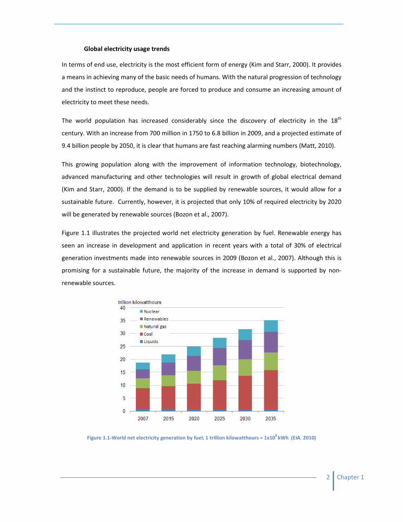
Figure 1.1 illustrates the projected world net electricity generation by fuel. Renewable energy has

seen an increase in development and application in recent years with a total of 30% of electrical

generation investments made into renewable sources in 2009 (Bozon et al., 2007). Although this is

promising for a sustainable future, the majority of the increase in demand is supported by non-

renewable sources.

Figure 1.1-World net electricity generation by fuel; 1 trillion kilowatthours = 1x109

kWh (EIA, 2010)

3 Chapter 1

Not only will the unprecedented consumption of these resources result in their eventual depletion,

but the burning of fuel contributes considerably to the emission of green house gases (GHG) and

ecological problems (IEA, 2009).

Carbon dioxide (CO2) is among the greenhouse gases which cause global warming. Since the

beginning of the industrial revolution, the burning of fossil fuels for energy has substantially

increased the amount of CO2 in the atmosphere. Energy production is responsible for 65% of global

CO2 emissions and is considered as a prime culprit in the global warming crisis (IEA, 2009).

With a dilemma between sustaining development, providing basic needs, and ecological

degradation, there is a great need for improving the manner in which energy is created and used.

This relies strongly on the strategies of both the consumer and the provider.

South African electricity situation

Eskom is the state-owned utility that provides South Africa with grid-electricity. It produces

approximately 95% of electricity used in South Africa and 45% of electricity used in Africa through

the Southern African Power Pool (Eskom, 2009).

In 2009 Eskom had a nominal generation capacity of 44 193 MW making it the largest producer of

electricity in Africa and among the top seven utilities in the world in terms of generation capacity.

Eskom was also among the top nine utilities in terms of electrical sales (Eskom, 2009).

Through the Integrated National Electrification Programme (INEP) of the Department of Minerals

and Energy, Eskom has been committed to the electrification of households, clinics, and schools of

previously disadvantaged communities. Since the beginning of the programme, approximately

4.9 million households, 163 clinics and 4957 schools have been electrified (DME, 2009).

As a result of such programmes, as well as the country’s economic growth, South Africa’s electrical

demand has increased considerably in the last decade. Figure 1.2 illustrates this growth in

comparison to maximum electrical generation capacity. As can be seen, the maximum demand has

been encroaching on the net maximum capacity, while reserve storage margin has become smaller.

4 Chapter 1

Figure 1.2-Generation plant capacity and maximum demand (Eskom, 2009)

In 2008 the consequence of operating a power system with a limited reserve margin was realised

when Eskom was forced to introduce load shedding. This is the systematic interruption of electrical

supply to different locations to reduce total demand. The electricity shortage was rotated between

locations to ensure that not only a few areas bore the brunt of the impact. If the trend line in Figure

1.2 continues without intervention, electrical demand would begin to exceed maximum capacity and

would result in a power system failure.

Many supply-side initiatives have been introduced by Eskom to assist in avoiding this under capacity

in the future. Several of these measures, such as the re-commissioning of power stations, will

possibly become operational only in 2012 (Eskom, 2009). Until then, a reduction in demand on the

system needs to be achieved. A number of recovery and purchasing programmes have been

undertaken to increase capacity and reduce the demand in the short term.

Eskom’s new build and recovery programmes

Under the new build and recovery programme, Eskom aims to increase its supply-side capacity. This

includes co-generation, the building of two open-cycle gas turbines and the reopening of three

power stations that were “mothballed” in the 1990’s (Eskom, 2009).

Co-generation is the encouragement of third parties to generate electricity for sale to the national

grid. This includes the Pilot National Co-generators Programme and the Medium-Term Power

Purchase Programme (Eskom, 2009). These resort under a power purchase agreement and cater for

a wide variety of technologies and contribution sizes starting from 5 MW up to a total of 3000 MW

(Eskom, 2009). Since the recommissioning of the mothballed power stations started in 2005, an

5 Chapter 1

additional capacity of 4,454 MW has been achieved, while the open-cycle gas turbines provide an

additional 150 MW each (Eskom, 2009). All of these contributed significantly to the alleviation of the

2008 electricity shortage.

In response to immense electricity challenges experienced in January 2008, Eskom established a

short term Stability and Recovery Programme (Eskom, 2009). This was divided into three phases;

phase 1, was to stabilise the supply demand for electricity; phase 2 involves re-establishing an

adequate reserve margin by managing demand; and phase 3 involves the plan to establish a

sustained load reduction through the Power Conservation Programme (PCP) (Eskom, 2009).

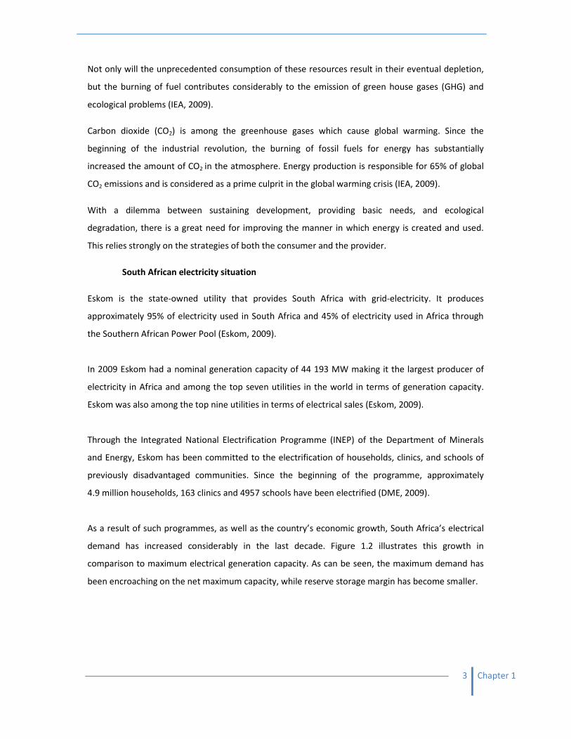
Phases 1 and 2 of the recovery programme saw the introduction of load shedding. The impact of the

limited supply caused a shift in electrical energy saving behaviour of South Africans. In promotion of

this shift, national power alerts, such as shown in Figure 1.3, were aired on national television. This

provided awareness among consumers and assisted in the recovery of the Eskom power system

between January 2008 and October 2008 (Eskom, 2009).

Figure 1.3-National power alert (Eskom, 2009)

Phase 3 involved the introduction of Demand Side Management (DSM) in order to establish a

sustainable reduction in load. This will be discussed in the following section.

Demand Side Management (DSM)

DSM is the programme by which Eskom aims to modify the electrical demand profile of the country.

Through a comprehensive implementation of available electricity and supervision of customer use, it

aims to reduce large “peaks” and “dips” in the electricity flow.

The typical daily demand profile for 2008 can be seen in Figure 1.4. The profile illustrates the large

peaks and dips in concern for DSM. In times of peak electricity usage, between 19:00 and 21:00,

Eskom needs the capacity to generate enough electricity to meet the needs of the consumers.

However, when the peaks reduce, the load on some power stations have to be reduced dramatically

before it has to be increased for the next peak. This is a complex control issue and an unwise

utilisation of resources.

6 Chapter 1

Figure 1.4-Electricity demand patterns, 14 July 2008 (Eskom, 2009)

Therefore, DSM aims to install energy-efficient technologies to reduce and alter the demand profile.

In the short term, DSM provides a measure to reduce the severity of the peaks and reduce costs of

expensive peaking plants. In the long run, it is an alternative to future extensive supply-side

investments. DSM aims to achieve a reduction in peak demand of 3000 MW by March 2011 and a

further 5000 MW by March 2026 (Eskom, 2009).

To achieve DSM objectives, attention is paid to the different sectors of the electricity market. The pie

graph in Figure 1.5 illustrates the percentages of electricity usage per sector for 2008 (DME, 2008).

The main contributors are the residential, commercial, mining and industrial sectors of South Africa

and are therefore areas of focus.

Figure 1.5 - Sectorial percentage market share on electricity in 2008 (DME, 2009)

The sensitivity of the market to the residential sector became evident when a 2% drop in demand

was experienced in 2008 in reponse to the national power alert initiative (Eskom, 2009). Due to the

increased awareness, it was possible to promote the installation of energy saving equipment in all

7 Chapter 1

sectors. It is speculated that many DSM initiatives have been initiating a culture of energy saving

throughout South Africa.

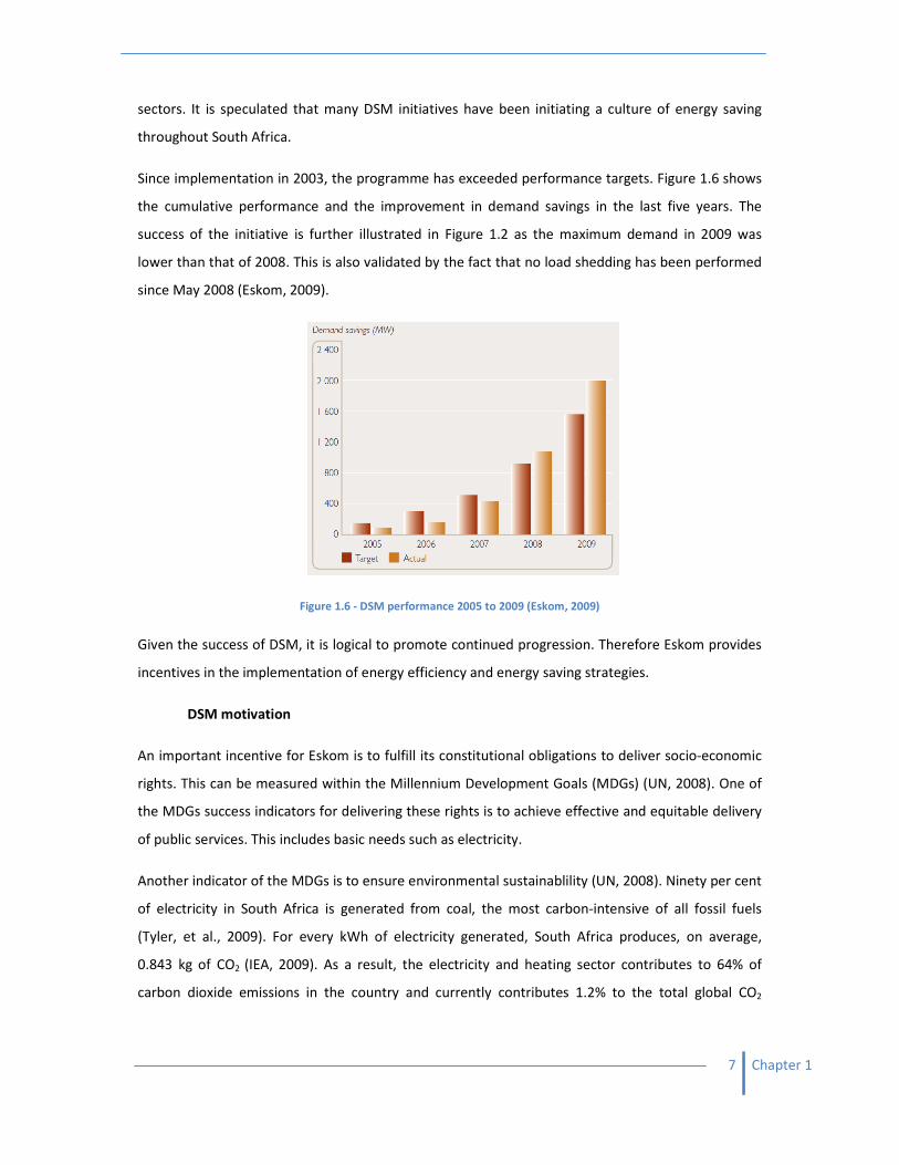
Since implementation in 2003, the programme has exceeded performance targets. Figure 1.6 shows

the cumulative performance and the improvement in demand savings in the last five years. The

success of the initiative is further illustrated in Figure 1.2 as the maximum demand in 2009 was

lower than that of 2008. This is also validated by the fact that no load shedding has been performed

since May 2008 (Eskom, 2009).

Figure 1.6 - DSM performance 2005 to 2009 (Eskom, 2009)

Given the success of DSM, it is logical to promote continued progression. Therefore Eskom provides

incentives in the implementation of energy efficiency and energy saving strategies.

DSM motivation

An important incentive for Eskom is to fulfill its constitutional obligations to deliver socio-economic

rights. This can be measured within the Millennium Development Goals (MDGs) (UN, 2008). One of

the MDGs success indicators for delivering these rights is to achieve effective and equitable delivery

of public services. This includes basic needs such as electricity.

Another indicator of the MDGs is to ensure environmental sustainablility (UN, 2008). Ninety per cent

of electricity in South Africa is generated from coal, the most carbon-intensive of all fossil fuels

(Tyler, et al., 2009). For every kWh of electricity generated, South Africa produces, on average,

0.843 kg of CO2 (IEA, 2009). As a result, the electricity and heating sector contributes to 64% of

carbon dioxide emissions in the country and currently contributes 1.2% to the total global CO2

8 Chapter 1

emissions (IEA, 2009). By reducing the demand for electricity and making provision for future

efficiency, Eskom can reduce its carbon footprint in global industry.

Consumers experience the same incentive for preserving the environment. With increased

awareness of global warming and green house gases, an increasing number of people are changing

their lifestyles to save energy. This natural incentive for people will motivate and promote the

energy efficiency that Eskom strives for.

In addition to global ecological preservation, financial incentives play a strong role in initiating

energy efficiency. Increases above inflation were needed, by Eskom, to fund capacity expansion. As a

result, the cost of electricity increased by 31.3% in 2009 and a further 24.8% in April 2010 (Lourens

and Seria, 2010). This enormous increase made electricity a much more expensive commodity for

South African consumers in comparison to previous years.

In addition to the overall increase, Eskom charges different tariffs at different times of the day to

better reflect the costs of electricity generation for its larger customers. This is because additional

peak-time generators are required during high consumption periods and are expensive to run, such

as the open cycle gas turbines which operate on diesel fuel. The tariffs are higher during these times

of peak demand and are further increased during winter periods when the demand is higher in

general.

In response to the increase in cost, consumers are trying to use electricity more wisely to save

money. This goes in hand with avoiding the prospect of load-shedding. After the 2008 load-shedding

programme, South Africans were made aware of the consequences of reckless energy use, and as

load-shedding is still a prospect until 2013, consumers are motivated into saving electricity to avoid

further disruption by load-shedding.

As the attitudes of South Africans are directed towards electricity savings, the method by which they

achieve it can be through DSM initiative programmes. Some of these are discussed in the following

sections.

DSM initiatives in the residential sector

In many countries, an area highlighted to have significant potential for electrical savings is the

domestic/residential sector (Clinch, 2001).

9 Chapter 1

To reduce consumption in the residential sector, Eskom implemented a mass roll out of 19 million

compact fluorescent lamps (CFL). This entailed the free exchange of incandescent light bulbs for CFL

across the country, as they typically use five times less electricity. The programme contributed to

389.9 MW of savings in 2008 and implementation continued until May 2010 (Eskom, 2009).

In other DSM programmes aimed at the residential sector, Eskom encourages the spread of the

energy burden to other sources of energy. Many campaigns and competitions have been run to

promote the use of solar water heaters and liquid petroleum gas for cooking. Other initiatives

included the implementation of efficient shower heads and smart electricity meters.

Due to the increased awareness of South Africans, business opportunities improved for companies

that provide solutions to consumers looking to implement energy savings projects. Such

corporations are known as energy service companies (ESCOs).

Energy service companies and their project scopes

ESCOs employ a form of outsourcing to design and implement energy savings projects for a broad

range of comprehensive energy solutions. They can provide a cost effective route to overcome

barriers in energy efficiency and DSM.

The ESCO analyses the consumer’s property, creates an energy efficiency solution, installs the

required equipment and maintains the system until the end of the contract or payback period. The

risk of the project is transferred from the consumer to the ESCO while they reduce operating costs.

This results in the production of valuable private energy saving projects in large industrial and

commercial consumers (Eskom, 2009).

The scope of the ESCO contract is defined by what the customer requires in terms of technologies

and systems. An illustration of such requirements can be seen in Figure 1.7. An ESCO can be involved

in total energy management from the import of energy to the final end use, or only subsections of

the system, such as a supply contract on the delivered energy or a performance contract on the

energy service (Sorrell, 2007). This would determine to what degree savings are achievable and also

the payback period of the contract.

10 Chapter 1

Figure 1.7-Scope of an energy service company. Adapted from Sorrell (2007)

DSM initiatives in industrial, commercial and mining sectors

The selling of DSM projects to consumers in the business sector may be difficult to achieve for

ESCOs. This is because there is a low return on investment in terms of monthly electrical bill savings

(Eskom, 2004a). Therefore, Eskom established the Industrial and Commercial Energy Efficiency (ICEE)

and Load Management (ICLM) initiatives. These ensure that participants receive benefits from the

installation of energy efficient technology and load management systems (Eskom, 2004b).

Energy efficiency aims at using less energy to achieve the same outcome as previously, thereby

reducing overall electrical consumption. Load management projects help to reduce only peak time

usage by either load-shifting or peak clipping. These spread the consumer electrical baseline more

evenly over the daily demand profile or improve utilisation of cheaper off-peak tariffs (Orans, et al.,

2010). Projects such as these are funded 100% by Eskom (Eskom, 2004b).

Eskom has agreed to fund, either partially or fully, the equipment that leads directly to energy

reduction. This depends on the type of savings achieved. DSM is about saving MW’s through load-

shifting and MWh’s through energy efficiency. This is the only deliverable for ESCOs and therefore

the equipment that is installed is the means to achieve the saving targets (Eskom, 2004a).

Energy efficiency projects help to reduce the entire baseline of the consumer. Fifty per cent of the

capital expenditure (capex) must be paid by the client benefiting from the equipment. Eskom covers

the remaining capex, as well as 100% of operation expenditure (opex) and measurement and

verification (M&V) costs (Eskom, 2004b).

11 Chapter 1

After the installation of the equipment, the client assumes ownership of all assets and the ESCO is

responsible for the maintenance of the project to ensure sustainability until the end of the useful life

time of the project (Eskom, 2004b).

Through these DSM initiatives, Eskom can reduce the rate of increase in the carbon footprint due to

South African electrical consumption. An improved generation capacity can then be projected. As a

result DSM projects should be promoted and conducted for economical and ecological sustainability

for both the country and the globe.

1.2. Motivation for this study

South Africa has large reserves of minerals which are found to be a primary source of energy and

trade. For example, the country has 3.7% of the total world coal resources for 2010 (BP, 2010). In

2003 South Africa was the fifth largest coal producing country in the world, and was the fourth

largest coal exporter (WCI, 2009). The industry is therefore dominated by large-scale minerals

extraction and processing.

The energy intensive nature of this minerals extraction and processing results in large quantities of

energy being used per unit of value produced. For this reason, a significant fraction of production

costs is taken up by energy purchases. By reducing energy costs, industries are able to increase their

profit and the financial incentives for conducting a DSM project are made apparent.

South African energy saving case study

To provide an example of the possible energy efficiency opportunities and their significant savings,

the following case study is presented.

The Energy Research Institute of the University of Cape Town was approached by a non-disclosed

South African manufacturing company to conduct an energy assessment. The assessment comprised

of energy conservation opportunities (ECO) and their respective savings and payback periods

(Fawkes, 2005). A summary of the assessment can be seen in Table 1.1.

Results showed that approximately R10.7 million could be saved per annum, amounting to 25% of

total energy costs with a short payback period of the capital required of 0.82 years (Fawkes, 2005).

This illustrates that there is enormous opportunity for energy savings should one consider an

appropriate industry.

12 Chapter 1

Table 1.1 - Energy conservation opportunities, with associated savings, implementation costs and payback periods

(Fawkes, 2005)

Eco Description

Potential

savings

(R/year)

Implementation

cost (R)

Payback

period

(years)

1 Repair compressed air leaks and faulty blow-

down valves to achieve 10% leakage targets 1 262 000 60 000 0.04

2 Avoid and discourage misuse of compressed air 263 189 30 000 0.11

3 Switch off compressors and maintain cooling

towers during non-production time 268 075 0 0

4 Install suitable power factor correction

equipment 516 690 1 007 500 2

5 Use waste heat to heat phosphate bath 190 000 300 000 1.58

6 Install high-efficiency lighting 179 803 628 198 3.4

7 Turn off bay lights during non-production hours 446 190 0 0

8 Install direct acting electric heaters to air

replacement plants 4 355 536 4 000 000 0.92

9

Make use of heat pump heat recovery between

air replacement plant exhaust and supply air

streams

3 187 385 2 750 000 0.87

Total 10 668 868 8 775 698 0.82

Determining the value of a DSM investigation

When an ESCO is approached to conduct an energy cost savings investigation, there is a need to

establish whether the DSM project is worth the investment. Company features, such as market

share, flexibility of production lines, ease of implementation, and others can be used to determine

the potential of DSM interventions. Howells (2006) conducted a study to develop a ranking for

industrial sectors according to these features. For the present study, the author was approached by

a South African cement production company to conduct an energy cost savings investigation.

The classification of cement production resorts in the class of non-metallic minerals processing,

along with brick making and others. Figure 1.8 illustrates the portions of electrical consumption in

the industrial and mining sectors for 2003. As can be seen, non-metallic minerals processing holds a

5% share, and as a result is ranked as seventh for overall electrical consumption (Howells, 2006).

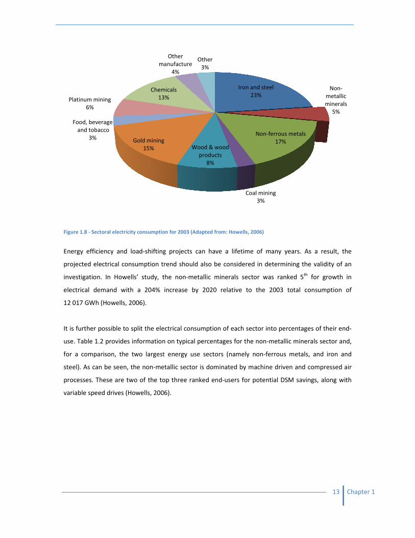
Figure 1.8 - Sectoral electricity consumption for 2003 (Adapted from:

Energy efficiency and load-shifting projects can have

projected electrical consumption trend should also be considered in determining the validity o

investigation. In Howells’ study, the non

electrical demand with a 204% increase by 2020 relative to the 2003 total consumption of

12 017 GWh (Howells, 2006).

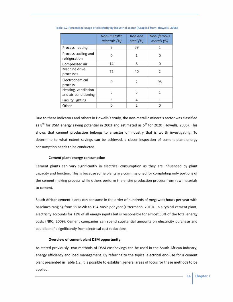
It is further possible to split the electrical consumption of each sector into percentages

use. Table 1.2 provides information on typical percentages for the non

for a comparison, the two largest energy use sectors

steel). As can be seen, the non-metallic sector is dominated by machine drive

processes. These are two of the top three ranked end

variable speed drives (Howells, 2006).

Gold mining

15%

Food, beverage

and tobacco

3%

Platinum mining

6%

Chemicals

13%

manufacture

on for 2003 (Adapted from: Howells, 2006)

shifting projects can have a lifetime of many years. As a result, the

projected electrical consumption trend should also be considered in determining the validity o

study, the non-metallic minerals sector was ranked 5th


electrical consumption of each sector into percentages

ovides information on typical percentages for the non-metallic minerals sector

largest energy use sectors (namely non-ferrous metals,

metallic sector is dominated by machine driven and compressed air

. These are two of the top three ranked end-users for potential DSM savings,

(Howells, 2006).

Iron and steel

23%

Non-ferrous metals

17%

Coal mining

3%

Wood & wood

products

8%

Gold mining

Chemicals

13%

Other

manufacture

4%

Other

3%

13 Chapter 1

years. As a result, the

projected electrical consumption trend should also be considered in determining the validity of an

for growth in


electrical consumption of each sector into percentages of their end-

metallic minerals sector and,

, and iron and

and compressed air

savings, along with

Non-

metallic

minerals

5%

14 Chapter 1

Table 1.2-Percentage usage of electricity by industrial sector (Adapted from: Howells, 2006)

Non- metallic

minerals (%)

Iron and

steel (%)

Non- ferrous

metals (%)

Process heating 8 39 1

Process cooling and

refrigeration 0 1 0

Compressed air 14 8 0

Machine drive

processes 72 40 2

Electrochemical

process 0 2 95

Heating, ventilation

and air-conditioning 3 3 1

Facility lighting 3 4 1

Other 0 2 0

Due to these indicators and others in Howells’s study, the non-metallic minerals sector was classified

as 8th

for DSM energy saving potential in 2003 and estimated as 5th

for 2020 (Howells, 2006). This

shows that cement production belongs to a sector of industry that is worth investigating. To

determine to what extent savings can be achieved, a closer inspection of cement plant energy

consumption needs to be conducted.

Cement plant energy consumption

Cement plants can vary significantly in electrical consumption as they are influenced by plant

capacity and function. This is because some plants are commissioned for completing only portions of

the cement making process while others perform the entire production process from raw materials

to cement.

South African cement plants can consume in the order of hundreds of megawatt hours per year with

baselines ranging from 55 MWh to 194 MWh per year (Ottermann, 2010). In a typical cement plant,

electricity accounts for 13% of all energy inputs but is responsible for almost 50% of the total energy

costs (NRC, 2009). Cement companies can spend substantial amounts on electricity purchase and

could benefit significantly from electrical cost reductions.

Overview of cement plant DSM opportunity

As stated previously, two methods of DSM cost savings can be used in the South African industry;

energy efficiency and load management. By referring to the typical electrical end-use for a cement

plant presented in Table 1.2, it is possible to establish general areas of focus for these methods to be

applied.

15 Chapter 1

As noted, the major portion of the electrical demand is taken by machine driven processes. In

cement plants these are commonly involved in driving fans, crushers, mills, conveyors, compressors

and turning kilns. This indicates, that should it be possible to implement a DSM programme to this

one area of focus, it would provide great savings to the total electrical consumption of a plant.

Currently, electric motors and their associated systems account for 60% of South African electricity

consumption (Eskom, 2008b). As this is recognised by Eskom, an Energy Efficient Motors Programme

was initiated to create awareness of the impact motors can have on national electricity savings.

Following this initiative it may be advantageous to investigate the improvement of energy efficiency

of machine driven processes in the plant.

When considering this possibility, constraints have been presented by Hughes (2006) at an energy

conference. He proposed that opportunity for improving motor efficiency in the cement industry is

limited due to the specialised nature of the motors and the extremely dusty environment in which

they operate. It is worthy to consider these perspectives and conduct further investigations into a

particular cement plant to establish the limitations.

To determine whether the load management method of savings is possible, it is necessary to

consider the basic processes of a cement plant. One needs to understand flow rates of materials,

limitations of equipment, minimum production rates, quality constraints and many other aspects.

This is to determine whether the production process provides flexibility during operating hours in

which to apply load-shifting. For example: as in many non-metallic materials processing, the kiln is

the slowest process of the cement making procedure. Therefore, there is a possibility to shift the

electric motors’ load before and after the kiln into periods with lower electrical tariffs, should the

productivity of the kiln allow this. This would reduce peak time energy purchase and therefore

reduce costs.

An investigation into these possibilities needs to be conducted to establish the availability for load

management in the production and opportunity for energy efficiency of electric motors. Again

referring to the end-use breakdown, other DSM opportunities may be found in compressed air

management; heating processes; heating, ventilation, air conditioning; and lighting control. All of

these could reduce electrical consumption of a plant should it be economically viable. These

opportunities should be investigated to determine their validity and potential savings.

16 Chapter 1

1.3. Objectives of the study

The primary objective for this study is to establish DSM opportunities within a typical South African

cement plant. Specifically, energy efficiency opportunities relevant to the country’s cement industry

will be investigated. The work will focus on load-shifting in an attempt to reduce peak-time

consumption and energy costs.

1.4. Scope of the study

Energy efficiency options in the cement industry will be investigated and the validity for the South

African industry will be examined. The emphasis of the work will however be on energy

management in the form of load-shifting.

To determine a viable load-shifting scheme, the study will optimise operating hours in typical

cement plant mills. This is to reduce the amount of electricity consumption during Eskom’s peak

period while maintaining production rates and standard time consumption.

1.5. Layout of dissertation

Chapter 1 provides a background to the study. This includes an overview of the global and national

electricity consumption problems and the environmental impact and, motivation and opportunities

behind conducting DSM initiatives in the cement production industry.

Chapter 2 investigates the state-of-the-art in energy efficiency and cost saving opportunities at

cement plants. Comparisons are made to establish viable options for typical South African cement

plants.

Chapter 3 investigates the operation of a typical cement plant. Historical data on production is used

in simulations to determine load-shifting options for the plant.

Chapter 4 provides results of a pilot study conducted on a plant with the load-shifting scheme

developed in Chapter 3.

Chapter 5 concludes the study with recommendations for viable DSM opportunities for a typical

South African cement plant.

17 Chapter 1

1.6. References

Alam, M., Bala, B., Huo, A., Matin, M., 1991. A model for the quality of life as a function of electrical

energy consumption. Energy 16 (4), 739-745.

Bozon, I.J.H., Campbell, W.J., Lindstrand, M., 2007. Global trends in energy. McKinsey Quarterly,

February 2007.

BP [British Petroleum], 2010. Statistical Review of World Energy June 2010. bp.com/

Statisticalreview. (Accessed on: October 2010)

Clinch, J.P., Healy, J.D., 2001. Cost-benefit analysis of domestic energy efficiency. Energy Policy 29

(2), 113-124.

DME [Department of Minerals and Energy], 2008. National Response to South Africa’s Electricity

Shortage. South African Government, Private Bag X19, Arcadia, 0007.

DME [Department of Minerals and Energy], 2009. Electrification Statistics 2009. South African

Government, Private Bag X19, Arcadia, 0007.

EIA [Energy Information Administration], 2010. International Energy Outlook 2010 – Highlights.

Independent Statistics and Analysis, United States.

Eskom, 2004a. The 12 Commandments for Energy Service Companies (ESCOs). Eskom, PO Box 1091,

Johannesburg, 2000, South Africa. www.eskomdsm.co.za/sites/default/files/u1

/12CommandESCOg.pdf (Accessed on: July 2010)

Eskom, 2004b. Demand Side Management’s Project Information Guide. Eskom, PO Box 1091,

Johannesburg,2000, South Africa. http://dsm.eskom.co.za/standardisation

/esco_guidev8.pdf (Accessed on: July 2010)

Eskom, 2008a. Eskom Annual Report 2008. Eskom, PO Box 1091, Johannesburg, 2000, South Africa.

Eskom, 2008b. Energy efficiency and demand side management programme overview 2008. Eskom,

PO Box 1091, Johannesburg, 2000, South Africa.

Eskom, 2009. Eskom Annual Report 2009. Eskom, PO Box 1091, Johannesburg, 2000, South Africa.

Fawkes, H., 2005. Energy Efficiency in South African Industry. Journal of Energy in Southern Africa 16

(4), 18-25.

Howells, M. I. 2006. The targeting of industrial energy audits for DSM planning. Journal of Energy in

Southern Africa 17 (1), 58-65.

Hughes, A., Howells, M.I., Trikam, A., Kenny, A.R., Van ES, D., 2006. A study of demand side

management potential in South African industries. Industrial and Commercial Use of Energy

Conference. University of Cape Town, Cape Town, South Africa.

IEA [International Energy Agency], 2009. CO2 emissions from fuel combustion – highlights (2009

Edition). France.

18 Chapter 1

Kim, J., Starr, C., 2000. Global Electrification and Nuclear Power: Toward Sustainable Growth in the

New Millennium. Progress in Nuclear Energy 37 (4), 1-18.

Lourens, C., Seria, N., 2010. South Africa to Lift Electricity Tariffs by 24.8% (Update 3), Bloomberg

Business Week, 24 February 2010.

NRC [Natural Resources Canada], 2009. Canadian cement industry energy benchmarking summary

report. Canadian Industry Programme for Energy Conservation. c/o Natural Resources

Canada, 580 Booth Street, 12th

floor, Ottawa, ON, K1A 0E4.

Orans, R., Woo, C.L., Horii, B., Chait, M., DeBenedicits, A., 2010. Electricity Pricing for Conservation

and Load-shifting. The Electricity Journal 23 (3), 7-14.

Otterman, E., 2010. Personnel communication with group energy manager at PPC head office. PPC

Building, 180 Katherine Street, Barlow Park Extention, Sandton, Johannesburg, South Africa.

Rosenberg, M., 2010. Current World Population. http://geography.about.com/od/

obtainpopulationdata/a/worldpopulation.htm (Accessed 22 June 2010).

Sheffield, J., 1998. World Population Growth and the Role of Annual Energy Use per Capita.

Technological Forecasting and Social Change 59 (1), 55-87.

Sorrell, S., 2007. The economics of energy service contracts. Energy Policy 33 (1), 507-521.

Tyler, E., Dunn, Z., du Toit, M., 2009. Economics of Climate Change: Context and Concepts Related to

Mitigation, Energy Research Centre, University of Cape Town, South Africa.

UN [United Nations], 2008. High level event on the Millennium Development Goals, 25 September

2008. United Nations Headquarters, East 42nd Street, New York City, United States.

WCI [World Coal Institute], 2009. The Coal Resource: A Comprehensive Overview of Coal. 5th Floor,

Heddon House, 149 - 151 Regent Street, London, W1B 4JD, United Kingdom.

19 Chapter 2

Chapter 2

Energy efficiency and load-shifting

opportunities in the cement industry

2.1. South African cement production plants

To determine the opportunities in DSM savings within a cement plant, the cement making process

needs to be understood. This chapter provides an overview of the cement making process in South

Africa, including a description of equipment and the management skills involved.

The local industry will be compared with the global industry to establish where South Africa ranks

within the growing international trend of energy savings and ecological impact reduction. By

researching successful case studies of energy efficiency and load-shifting, both nationally and

internationally, it can be determined whether similar projects can be applied to the cement plant

under investigation.

20 Chapter 2

Portland cement

Cement is a bonding agent which hardens and binds building materials. It is usually a fine grey

powder and when mixed with water or other hydraulic material undergoes a chemical reaction. Over

time the mixture “dries out” and hardens. Depending on the type of cement, the conditions under

which the chemical reactions take place, can differ.

There are two types of cement: hydraulic, which is able to set under wet conditions, and non-

hydraulic, which needs to remain dry in order to harden. An example of the hydraulic type is

Portland cement and its various blends. The South African cement industry, which is currently

accountable for 0.57% of the World’s cement production, produces only Portland cement. It is

commonly used around the globe for its general use in concrete, mortars, stucco and grout (Tatum,

2010).

Portland cement consists primarily of limestone and other additives. Depending on the purity of the

limestone, secondary raw materials such as clay, chalk, shale, sand, iron ore and others may be

added to meet production standards (Hassaan, 2001).

Wet or dry processes are used for the production of Portland cement depending on characteristics

and availability of the raw materials used in the manufacture. Only the dry process is used in South

Africa.

Dry process cement production

Figure 2.1 illustrates the basic process taken during the dry production of Portland cement, and will

be briefly discussed.

Obtaining raw materials

Limestone is obtained from a mine or quarry usually situated close to the cement mill. It is then

transported to a crusher where is it crushed to smaller segments approximately 50mm in size. If

secondary raw material is needed, it is mixed together in a prehomogenising pile. To produce a good

quality product and to maintain efficient combustion conditions in the kiln, it is crucial that the raw

meal is completely homogenised.

21 Chapter 2

Figure 2.1 - Dry Process Cement Production. Adapted from Choate (2003)

22 Chapter 2

Raw mill and silo

The raw materials are then ground together in a raw mill. This is to reduce particle size into a fine

powder and form what is known as the raw meal. Four different types of mills may be used in this

stage, which varies from one cement production company to the next. There are ball mills,

consisting of a rotating horizontal cylinder partly filled with steel balls (NSI, 2010), vertical roller

mills, using vertical spindles on a rotary table (Alstom, 2010), hammer mills, which implement a shaft

mounted with hammers in a rotary drum (MS,2010), and high-pressure roll presses, which crushes

material between two rollers (ALF-Cemind, 2010). Figure 2.2 illustrate these mills.

Figure 2.2 - Types of mills. Adapted from NSI (2010), Alstom (2010) MS (2010) and ALF-Cemind (2007)

The material entering the mills may contain moisture and can form an undesirable mud as it is

crushed. To avoid this, hot air is blown through the mill from either a furnace or as waste gases from

the clinker kiln. This ensures that the raw meal created is in a dust-like composition.

Once a minimum particle size is reached it is possible for raw meal to pass through a particle size

separator or classifier. Classifiers separate the finely ground particles from the coarse particles. The

large particles are then recycled back to the mill. This can be achieved by, for example, blowing the

lighter dust particles through a series of screens. It may also be separated and collected by an

electrostatic precipitator, a device highly effective in filtration by means of an applied electrostatic

charge (Q-filter, 2010). The raw meal is then stored in a silo where it is monitored to stay within a

specified capacity level in the silo. It is then fed into the kiln.

23 Chapter 2

Preheating

The exhaust of hot gases from the kiln can be used to preheat the raw meal. This is to evaporate any

moisture that might have remained after the milling, or, that may have been absorbed from the

atmosphere during storage. It is also used for the beginning process of sintering the raw meal. The

material can be heated from 70°C to 800°C where de-carbonation can begin. This is where the

limestone releases carbon dioxide in the process of forming clinker, the main compound of cement

before it is ground (Wansbrough, 2008).

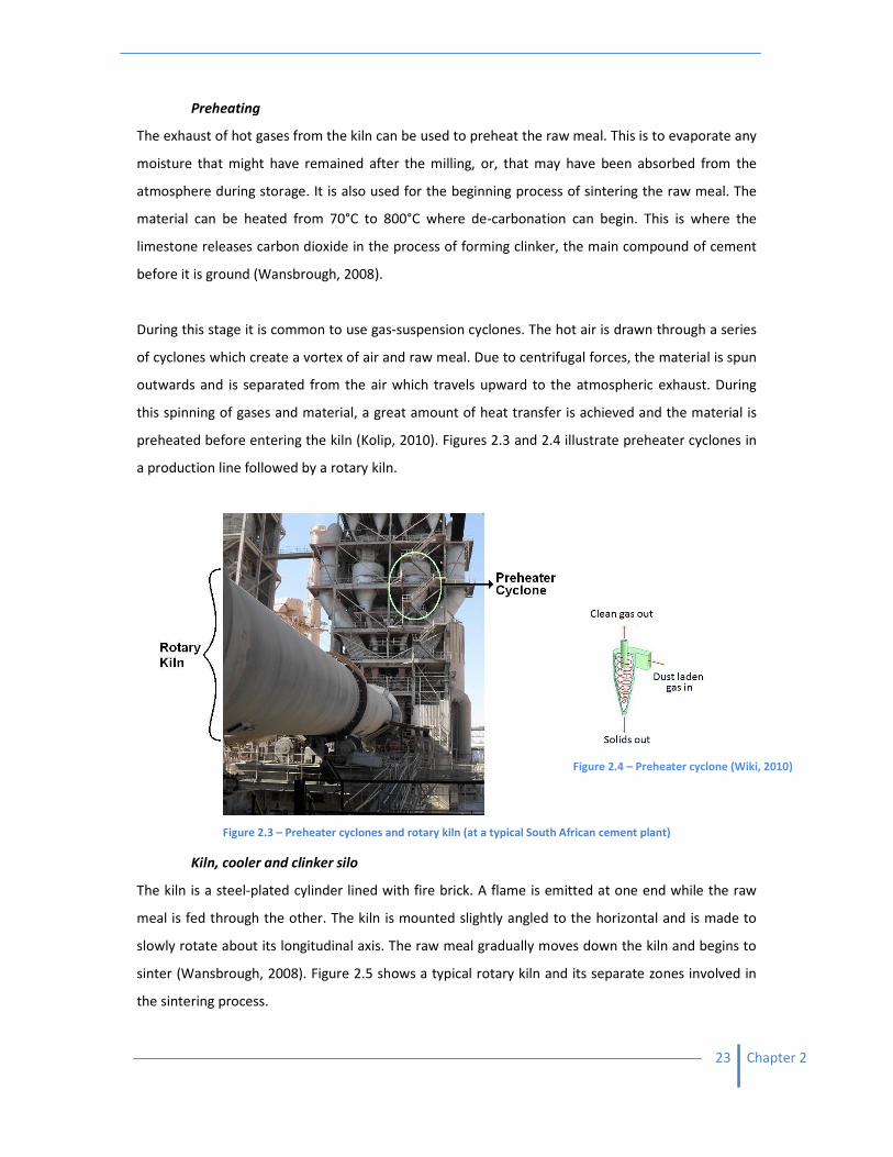
During this stage it is common to use gas-suspension cyclones. The hot air is drawn through a series

of cyclones which create a vortex of air and raw meal. Due to centrifugal forces, the material is spun

outwards and is separated from the air which travels upward to the atmospheric exhaust. During

this spinning of gases and material, a great amount of heat transfer is achieved and the material is

preheated before entering the kiln (Kolip, 2010). Figures 2.3 and 2.4 illustrate preheater cyclones in

a production line followed by a rotary kiln.

Figure 2.3 – Preheater cyclones and rotary kiln (at a typical South African cement plant)

Kiln, cooler and clinker silo

The kiln is a steel-plated cylinder lined with fire brick. A flame is emitted at one end while the raw

meal is fed through the other. The kiln is mounted slightly angled to the horizontal and is made to

slowly rotate about its longitudinal axis. The raw meal gradually moves down the kiln and begins to

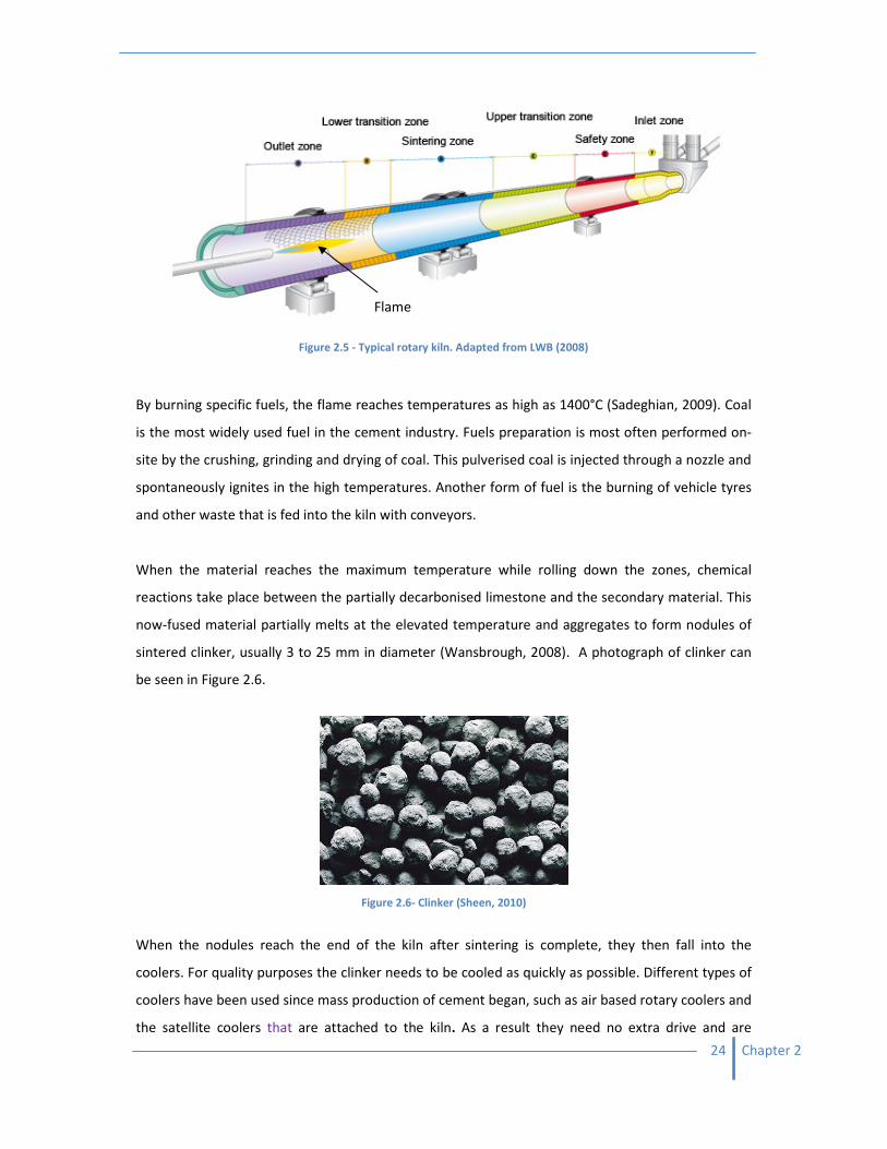
sinter (Wansbrough, 2008). Figure 2.5 shows a typical rotary kiln and its separate zones involved in

the sintering process.

Figure 2.4 – Preheater cyclone (Wiki, 2010)

24 Chapter 2

Figure 2.5 - Typical rotary kiln. Adapted from LWB (2008)

By burning specific fuels, the flame reaches temperatures as high as 1400°C (Sadeghian, 2009). Coal

is the most widely used fuel in the cement industry. Fuels preparation is most often performed on-

site by the crushing, grinding and drying of coal. This pulverised coal is injected through a nozzle and

spontaneously ignites in the high temperatures. Another form of fuel is the burning of vehicle tyres

and other waste that is fed into the kiln with conveyors.

When the material reaches the maximum temperature while rolling down the zones, chemical

reactions take place between the partially decarbonised limestone and the secondary material. This

now-fused material partially melts at the elevated temperature and aggregates to form nodules of

sintered clinker, usually 3 to 25 mm in diameter (Wansbrough, 2008). A photograph of clinker can

be seen in Figure 2.6.

Figure 2.6- Clinker (Sheen, 2010)

When the nodules reach the end of the kiln after sintering is complete, they then fall into the

coolers. For quality purposes the clinker needs to be cooled as quickly as possible. Different types of

coolers have been used since mass production of cement began, such as air based rotary coolers and

the satellite coolers that are attached to the kiln. As a result they need no extra drive and are

Flame

25 Chapter 2

therefore advantageous over stationary coolers. Due to their lower rate of cooling, however, they

have been replaced by grate coolers (UNIDO, 1994).

A grate cooler houses perforated plates that are able to slide back and forth. This shuffles the clinker

to the end of the cooler while air is blown through the perforated holes. The temperature of the

clinker is reduced to 100°C before it is transported to a silo to be stored (UNIDO, 1994).

The sintering process in the kiln is usually the slowest stage of manufacture. Often the capacity of

the kiln can determine the capacity of the plant. As a result, the kiln typically runs 24 hours, 7 days a

week, and the levels of clinker are closely monitored in the silo.

Cement/finishing mill

The clinker is transported from the silo and combined with a small quantity of gypsum and fly ash.

This is a material that retards the setting time of the cement. Quantities of gypsum and fly ash can

determine the characteristics of the cement and can qualify different grades (Kavas, et al., 2005). In

this final stage, the mixture is then ground together often using ball mills. As the mill drum rotates,

steel balls cascade onto the clinker and gypsum. Usually different sized steel balls are used in

succession and as the material passes through different chambers it is reduced gradually. This

crushes and mixes the material into the fine grey powder known as cement (UNIDO, 1994).

Cement silos and packaging

Once the particles are fine enough to pass product standards they are removed and stored in

cement silos. They are then packaged into cement bags or loaded for bulk transport in trucks or

trains. The cement mill is directly related to the production rate of the cement plant and is therefore

integral to the success of the plant.

To help maintain and control the processes around the plant, a supervisory control and data

acquisition (SCADA) system can be used to monitor performance. Examples of information that

could be captured by the system would be the flow rates of materials, motor power consumption,

operating hours, kiln temperature, level of silos and others.

To evaluate where energy efficiency and load-shedding can be applied during the production

process, one should comprehend processes which have a large demand for electricity.

2.2. Electrical consumption by department

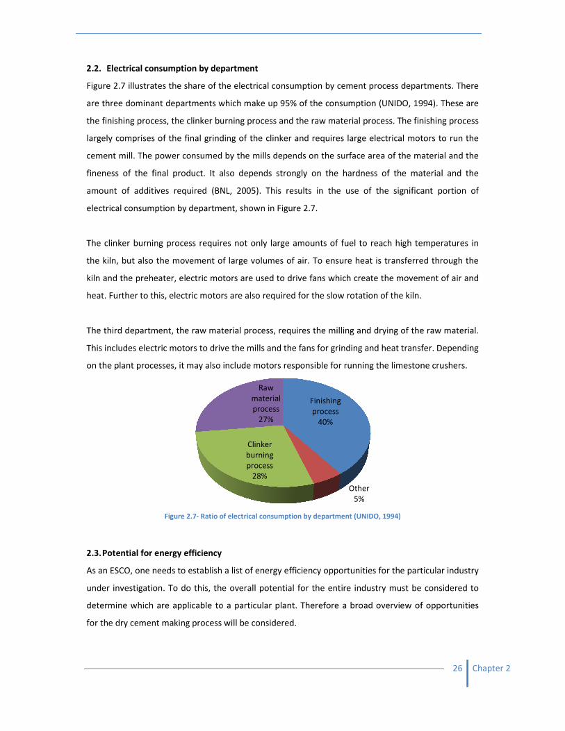
Figure 2.7 illustrates the share of the electrical consumption by

are three dominant departments which make up 95% of the

the finishing process, the clinker burning process and the raw material process. The finishing process

largely comprises of the final grinding of the clinker and requires large electrical motors to run the

cement mill. The power consumed by the mills depends on the surface area of the material and the

fineness of the final product. It also depends strongly on the hardness of the material a

amount of additives required (BNL, 2005). This results in the use of the significant portion of

electrical consumption by department, shown in Figure 2.7.

The clinker burning process requires not only large amounts of fuel to reach high temperatur

the kiln, but also the movement of large volumes of air. To ensure heat is tr

kiln and the preheater, electric motors are used to drive fans which create

heat. Further to this, electric motors are also req

The third department, the raw material process, requires the milling and drying of the raw material.

This includes electric motors to drive the mills and the fans for grinding and heat transfer. Depending

on the plant processes, it may also include motors responsible for running the limestone crushers.

Figure 2.7- Ratio of electrical consumption by department (UNIDO, 1994)

2.3. Potential for energy efficiency

As an ESCO, one needs to establish a list of energy

under investigation. To do this, the overall potential for the entire industry must be considered to

determine which are applicable to a particular plant. Therefore a broad overview of opportunities

for the dry cement making process will be considered.

Electrical consumption by department

illustrates the share of the electrical consumption by cement process departments. There

are three dominant departments which make up 95% of the consumption (UNIDO, 1994). These are


inding of the clinker and requires large electrical motors to run the


fineness of the final product. It also depends strongly on the hardness of the material a

(BNL, 2005). This results in the use of the significant portion of

electrical consumption by department, shown in Figure 2.7.

The clinker burning process requires not only large amounts of fuel to reach high temperatur

the kiln, but also the movement of large volumes of air. To ensure heat is transferred through the

motors are used to drive fans which create the movement of air and

Further to this, electric motors are also required for the slow rotation of the kiln.



processes, it may also include motors responsible for running the limestone crushers.

Ratio of electrical consumption by department (UNIDO, 1994)

As an ESCO, one needs to establish a list of energy efficiency opportunities for the particular industry



ing process will be considered.

Finishing

process

40%

Other

5%

Clinker

burning

process

28%

Raw

material

process

27%

26 Chapter 2

process departments. There

(UNIDO, 1994). These are


inding of the clinker and requires large electrical motors to run the


fineness of the final product. It also depends strongly on the hardness of the material and the

(BNL, 2005). This results in the use of the significant portion of

The clinker burning process requires not only large amounts of fuel to reach high temperatures in

ansferred through the

the movement of air and

for the slow rotation of the kiln.



processes, it may also include motors responsible for running the limestone crushers.

efficiency opportunities for the particular industry



27 Chapter 2

Overall potential classification

Energy efficiency opportunities can be classified into three general categories (KEMA, 2005). These

are listed below and brief examples for the cement industry are given:

1. High-efficiency equipment/processes - These involve modifications of major processes or

equipment that are industry-specific and highly specialised. For a cement plant, some

measures include: conversion of ball mills to roller mills for grinding, efficient materials

transport systems, high-efficiency classifiers, conversion to more efficient kilns such as

vertical precalciner kilns, variable speed drives (VSDs) for fans and other variable load drives,

and improvements in compressed air system used to transport and mix material.

2. Controls - These present opportunities for improving process controls involved in, for

example, clinker production and finish grinding, as well as operation of compressed air

systems, and the shifting of electrical load.

3. Observation and maintenance (O&M) - O&M energy efficiency includes projects such as

motor belt replacement, motor and bearing lubrication, fan blade cleaning, fan wheel

balancing, and compressed air system maintenance.

Energy efficiency opportunities in the cement industry

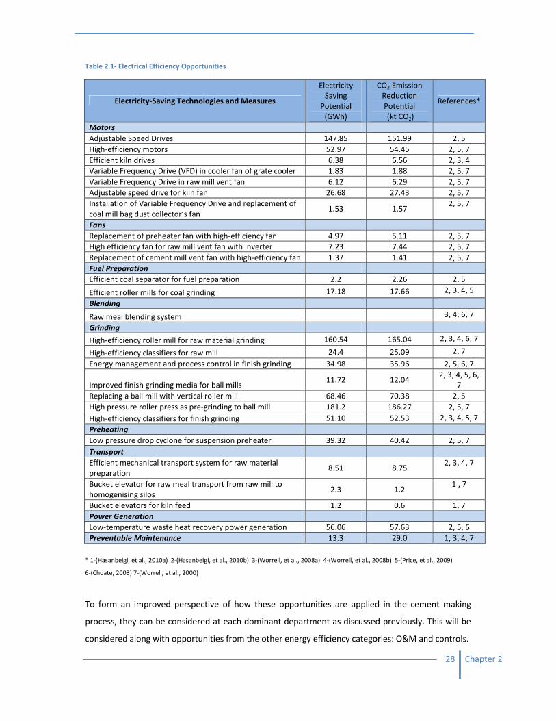
For the first category, high-efficiency equipment/processes, Table 2.1 presents a list of plausible

energy efficiency opportunities. These are established by a combination of case studies conducted

for the cement industry worldwide (Hasanbeigi, et al., 2010a, b; Worrell, et al., 2000, 2008a, b; Price,

et al., 2009; Choate, 2003). It includes the values of electricity savings potential and CO2 reduction

potential for two case studies in particular, Shandong Province, China (Hasanbeigi, et al., 2010b), and

Thailand (Hasanbeigi, et al., 2010a).

The table lists opportunities for both major and minor changes in equipment and processes for a

plant. For example, it includes the complete replacement of large machinery with higher efficiency

models as well as the upgrade of subsystems. At a later stage, the relevance of each opportunity to

the specific plant/s under investigation will be established.

28 Chapter 2

Table 2.1- Electrical Efficiency Opportunities

Electricity-Saving Technologies and Measures

Electricity

Saving

Potential

(GWh)

CO2 Emission

Reduction

Potential

(kt CO2)

References*

Motors

Adjustable Speed Drives 147.85 151.99 2, 5

High-efficiency motors 52.97 54.45 2, 5, 7

Efficient kiln drives 6.38 6.56 2, 3, 4

Variable Frequency Drive (VFD) in cooler fan of grate cooler 1.83 1.88 2, 5, 7

Variable Frequency Drive in raw mill vent fan 6.12 6.29 2, 5, 7

Adjustable speed drive for kiln fan 26.68 27.43 2, 5, 7

Installation of Variable Frequency Drive and replacement of

coal mill bag dust collector’s fan 1.53 1.57

2, 5, 7

Fans

Replacement of preheater fan with high-efficiency fan 4.97 5.11 2, 5, 7

High efficiency fan for raw mill vent fan with inverter 7.23 7.44 2, 5, 7

Replacement of cement mill vent fan with high-efficiency fan 1.37 1.41 2, 5, 7

Fuel Preparation

Efficient coal separator for fuel preparation 2.2 2.26 2, 5

Efficient roller mills for coal grinding 17.18 17.66 2, 3, 4, 5

Blending

Raw meal blending system

3, 4, 6, 7

Grinding

High-efficiency roller mill for raw material grinding 160.54 165.04 2, 3, 4, 6, 7

High-efficiency classifiers for raw mill 24.4 25.09 2, 7

Energy management and process control in finish grinding 34.98 35.96 2, 5, 6, 7

Improved finish grinding media for ball mills 11.72 12.04

2, 3, 4, 5, 6,

7

Replacing a ball mill with vertical roller mill 68.46 70.38 2, 5

High pressure roller press as pre-grinding to ball mill 181.2 186.27 2, 5, 7

High-efficiency classifiers for finish grinding 51.10 52.53 2, 3, 4, 5, 7

Preheating

Low pressure drop cyclone for suspension preheater 39.32 40.42 2, 5, 7

Transport

Efficient mechanical transport system for raw material

preparation 8.51 8.75

2, 3, 4, 7

Bucket elevator for raw meal transport from raw mill to

homogenising silos 2.3 1.2

1 , 7

Bucket elevators for kiln feed 1.2 0.6 1, 7

Power Generation

Low-temperature waste heat recovery power generation 56.06 57.63 2, 5, 6

Preventable Maintenance 13.3 29.0 1, 3, 4, 7

* 1-(Hasanbeigi, et al., 2010a) 2-(Hasanbeigi, et al., 2010b) 3-(Worrell, et al., 2008a) 4-(Worrell, et al., 2008b) 5-(Price, et al., 2009)

6-(Choate, 2003) 7-(Worrell, et al., 2000)

To form an improved perspective of how these opportunities are applied in the cement making

process, they can be considered at each dominant department as discussed previously. This will be

considered along with opportunities from the other energy efficiency categories: O&M and controls.

29 Chapter 2

Raw material process

1. Use of roller mills - It is customary to use ball mills for the grinding of the raw meal. These

can be replaced by high-efficiency roller mills, ball mills combined with high-pressure roller

presses, or vertical roller mills, to save energy without compromising quality. An additional

advantage of the inline vertical roller mills is that they can combine raw material drying with

the grinding process by using large quantities of low-grade waste heat from the kilns or

clinker coolers (Worrell, et al., 2008a).

2. Raw meal process control – A problem exists with vertical roller mills tripping as a result of

elevated vibration. Operation at high throughput makes manual vibration control difficult

and the mill can trip. When it does so, it cannot be re-started until the motor windings cool

down. A multivariable controller can manage total feed while maintaining a production

target and keep within a safe range for trip-level vibration (Worrell, et al., 2008a).

3. Raw meal blending (homogenising) systems - To blend the raw meal, most plants use

compressed air or use mechanical systems to agitate the powdered meal. A reduction in

electrical consumption can be found by converting to gravity-type homogenising silos. In

these silos, material funnels down one of many discharge points, where it is mixed in an

inverted cone. Table 2.2 lists the relative electrical consumption of the types of blenders

showing the large difference in demand (Fujimoto, 1993).

Table 2.2 - Comparison of homogenising systems (Fujimoto, 1993)

Homogenising system kWh/ton of raw meal

Mechanical system 2.00 - 2.50

Air fluidised system 1.00 - 1.50

Gravity - inverted cone 0.25 - 0.50

Gravity - multi outlet 0.10 - 0.13

4. Efficient transport systems - Transport systems are required to convey powdered materials

such as kiln feed, kiln dust, and finished cement throughout the plant. These materials are

usually transported by means of either pneumatic or mechanical conveyors. Conversion to

mechanical conveyors is cost-effective when replacement of conveyor systems is needed to

increase reliability and reduce downtime (Worrell, et al., 2008a).

5. High-efficiency classifiers/separators - A recent development in efficient grinding

technologies is the use of high-efficiency classifiers or separators. Standard classifiers may

have a low separation efficiency, which leads to the recycling of fine particles, and results in

extra power use in the grinding mill. High-efficiency classifiers can be used in both the raw

materials mill and in the finish grinding mill (Worrell, et al., 2008a).

30 Chapter 2

Clinker burning process

1. Adjustable speed drive for kiln fan - Adjustable or VSD for the kiln fan can result in reduced

electrical use and reduced maintenance costs (Worrell, et al., 2008a).

2. Efficient kiln drives - A substantial amount of power is used to rotate the kiln. High

efficiencies can be achieved using a single pinion drive with an air clutch and a synchronous

motor (Regitz, 1996). Also, the use of alternating current (AC) motors is advocated to replace

the traditionally used direct current (DC) drive. The AC motor system can result in 1.5%

higher efficiencies (Holland, 2001).

3. Other energy-efficiency technologies and measures have great potential for overall energy

savings. However, they do not have a direct influence on electricity demand. These include

kiln combustion system improvements, reciprocating grate coolers, optimising heat recovery

and upgrading the clinker cooler, seal replacement, low-temperature waste heat recovery

for power generation, high-temperature waste heat recovery for power generation, multi-

stage preheater/precalciner kiln and low pressure drop cyclones for suspension pre-heaters

(Worrell, et al., 2008a).

Finishing process (Worrell, et al., 2008a)

1. Process control and management - Improved systems control can be implemented to

monitor and maintain the flow in the cement mills and classifiers. This results in achieving a

stable and high quality product while avoiding unnecessary electricity consumption.

2. Advanced grinding concepts - Energy efficiency is relatively low for ball mills in finish

grinding. Several new mill concepts exist that can significantly reduce power consumption in

the finish mill, including roller presses, roller mills, and roller presses used for pre-grinding in

combination with ball mills. Roller mills employ a mix of compression and shearing to

pressurise the material, where ball mills adopt specific feed charge and particle size. Both

improve the grinding efficiency dramatically (Touil, et al., 2006). Today, high-pressure roller

presses are most often used to expand the capacity of existing grinding mills, and are found

especially in countries with high electricity costs or with poor power supply (Worrell, et al.,

2008a).

3. Improved grinding media - Improved wear resistant materials can be installed for grinding

media, especially in ball mills. Grinding media are usually selected according to the wear

characteristics of the material as there is potential for reducing wear as well as energy

consumption by increasing the ball charge distribution and surface hardness of grinding

media (Choate, 2003).

31 Chapter 2

4. High-efficiency classifiers - A recent development in efficient grinding technologies is the use

of high-efficiency classifiers or separators which have great impact on improving product

quality and reducing electricity consumption (Worrell, et al., 2008a).

Plant Wide Measures

1. Preventative maintenance - Preventative maintenance includes the training of personnel to

be attentive to energy consumption and- efficiency. While many processes in cement

production are primarily automated, there are still opportunities, requiring minimal training

of employees, to increase energy savings.

2. High-efficiency motors and drives - Motors and drives are used throughout a cement plant

to rotate the kiln, run fans, transport materials and grinding. In a typical cement plant, there

can be 500-700 electric motors in operation, ranging from a few kW to MW-size (Vleuten,

1994). By improving control strategies, installing variable speed drives or high-efficiency

motors, the power consumption of an entire plant can be reduced.

3. Compressed air systems - Compressed air systems are used for many different operations in

the plant, for example in mixing and transporting material, dust collector filters, packaging

and others. Total energy consumption by compressed air systems is relatively small in

comparison to drive systems; however, it can amount to an unnecessary expense if the

systems runs continuously and end-users are offline. In addition, compressed air is an

expensive commodity for its poor efficiency; therefore management and maintenance

systems can be implemented to minimise unnecessary expenses (Worrell, et al., 2008a).

4. Lighting – Energy efficiency in lighting can cost-effectively reduce energy consumption even

though energy used for lighting in the cement industry is relatively low.

2.4. Priorities and barriers in DSM initiatives

Although there are great opportunities for energy efficiency and energy cost savings, one may ask

why a cement company in particular might engage in the projects listed above. How important is

energy efficiency to cement companies and what prevents them from embarking on such projects?

By answering these questions, it would be possible to eliminate any inapplicable projects at a later

stage.

By employing ESCOs, companies are looking to improve company performance. By taking on such

measures, a cement plant can avoid future unnecessary costs, as well as governmental constraints.

For example, vertical shaft kilns (VSK) have a poorer efficiency than rotary kilns and may contribute

32 Chapter 2

to unnecessary energy consumption (Cho, et al., 2007). In an attempt to enforce energy efficiency of

the country’s cement plants, an official Chinese government policy was adopted in 2006 to phase

out VSK and completely replace them with more modern kilns (Hasanbeigi, et al., 2010b). However,

in 2010 nearly 40% of China’s cement plants still use VSK and the Chinese energy efficiency level

compared to the global benchmark is relatively low (Hasanbeigi, et al., 2010b).

As a result, cement output in China became restricted in several provinces as they adopted

electricity-use controls on cement producers from September to the end of December 2010. This is

to fulfil their energy-saving goal of reducing energy consumption per gross domestic profit unit by

20% before the end of 2010. Because of this, some provinces, such as Guangxi, had to cut cement

production by at least 50% and raise prices of cement by up to 30% (CC, 2010).

This would be detrimental to business and public relations. If more of the cement plants were able

to adopt the energy efficiency opportunities discussed previously, energy consumption may have

been lowered and such constraints may have been avoided.

In other cases, initiating electricity cost savings can be beneficial during economic recessions or

market declines. For example, a boom in South African cement sales was experienced in 2007 as

government invested in large infrastructure projects such as highways, the Gautrain, electricity

plants and dams (Lourens, 2007). This is in addition to the preparations undertaken for the South

African Fifa World Cup 2010, such as the construction of stadiums and airports (Mokopanele, 2010).

Since then, however, due to the completion of many of the projects, the cement industries in South

Africa have experienced a significant decline in sales (BD, 2010). The reduction in sales between

January 2007and October 2010 is illustrated in Figure 2.8.

Figure 2.8- Monthly average daily sales of Portland cement in South Africa and neighbouring countries (CNCI, 2009)

40000

45000

50000

55000

60000

65000

70000

Jan Feb Mar Apr May Jun Jul Aug Sep Oct Nov Dec

Sa

les

pe

r d

ay

(to

ns)

2007

2008

2009

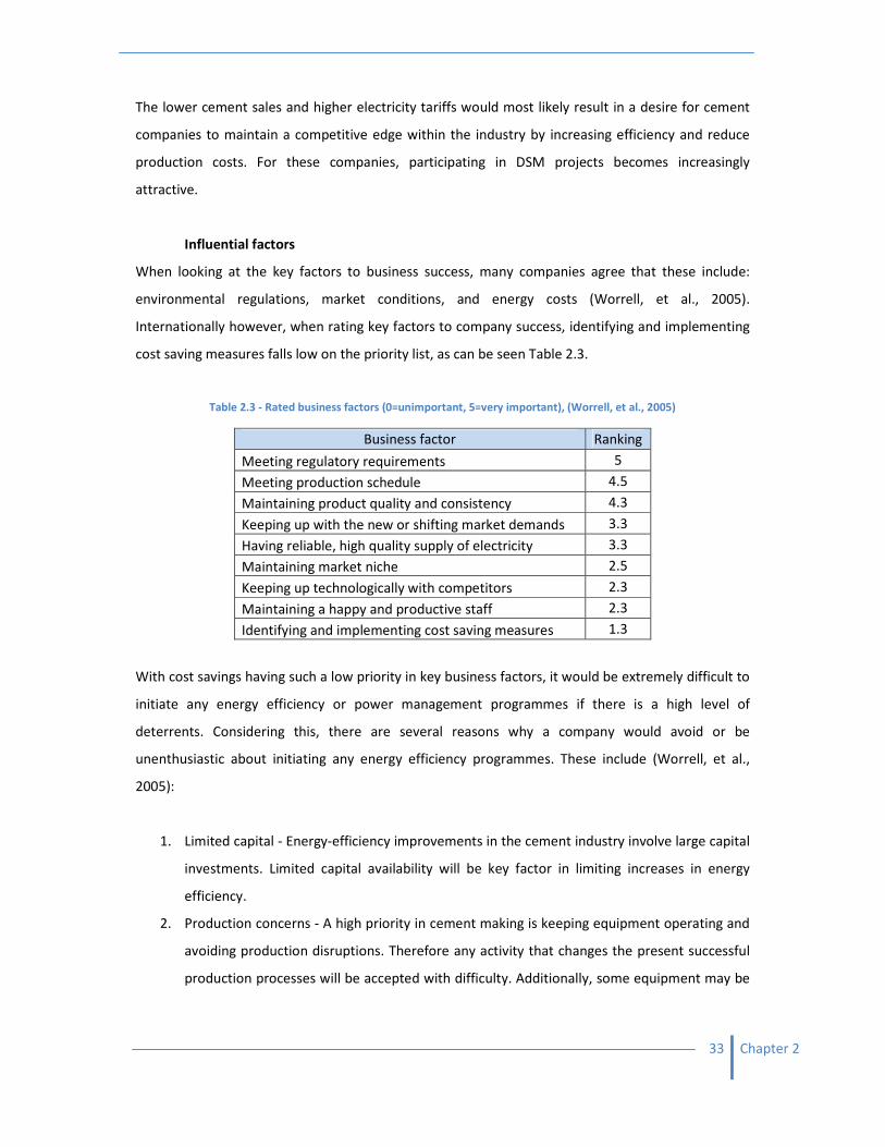
33 Chapter 2

The lower cement sales and higher electricity tariffs would most likely result in a desire for cement

companies to maintain a competitive edge within the industry by increasing efficiency and reduce

production costs. For these companies, participating in DSM projects becomes increasingly

attractive.

Influential factors

When looking at the key factors to business success, many companies agree that these include:

environmental regulations, market conditions, and energy costs (Worrell, et al., 2005).

Internationally however, when rating key factors to company success, identifying and implementing

cost saving measures falls low on the priority list, as can be seen Table 2.3.

Table 2.3 - Rated business factors (0=unimportant, 5=very important), (Worrell, et al., 2005)

Business factor Ranking

Meeting regulatory requirements 5

Meeting production schedule 4.5

Maintaining product quality and consistency 4.3

Keeping up with the new or shifting market demands 3.3

Having reliable, high quality supply of electricity 3.3

Maintaining market niche 2.5

Keeping up technologically with competitors 2.3

Maintaining a happy and productive staff 2.3

Identifying and implementing cost saving measures 1.3

With cost savings having such a low priority in key business factors, it would be extremely difficult to

initiate any energy efficiency or power management programmes if there is a high level of

deterrents. Considering this, there are several reasons why a company would avoid or be

unenthusiastic about initiating any energy efficiency programmes. These include (Worrell, et al.,

2005):

1. Limited capital - Energy-efficiency improvements in the cement industry involve large capital

investments. Limited capital availability will be key factor in limiting increases in energy

efficiency.

2. Production concerns - A high priority in cement making is keeping equipment operating and

avoiding production disruptions. Therefore any activity that changes the present successful

production processes will be accepted with difficulty. Additionally, some equipment may be

34 Chapter 2

damaged from recurring stoppages, such as stresses in the ceramic insulation of the kiln

during shutdown.

3. Limited staff time - implementing energy efficiency may require additional staff and staff

time. This will not be a priority over keeping production running.

4. Information - Information on energy-efficiency improvements is readily available. However it

may be time consuming to focus on the information and to make decisions.

5. Reliability concerns - Maintaining production is a high priority, therefore, cement making

companies may be concerned about the reliability of all new equipment.

6. Inconvenience - if staff time is limited, smaller energy-efficiency projects are not pursued

because they “are not worth the trouble.”

There may also be deterrents against a company working with an ESCO. These are (Worrell, et al.,

2005):

1. Short programme period - It can take three to five years for customers to develop and

implement a project. The time period may interfere with other plant plans or operations.

2. Limited incentives - many of the cement plant projects cost hundreds of millions of Rand.

Projects saving a few million Rand may not provide enough incentive.

3. M&V (measurement and verification) requirements - many M&V requirements have

favoured equipment change outs, where pre and post equipment efficiencies are easy to

measure. Projects that require more “holistic” measurement, and which affect energy use of

an entire system, are harder to justify savings and thus have limited acceptance.

4. Program administration: The collaboration with Eskom may deter companies from

participation in DSM projects as the protocol is time consuming and a burden on customer

staff.

The above adversely affect the validity of energy efficiency opportunities. They can determine

whether taking on an endeavour would be feasible. An evaluation process can help to establish

which opportunities are feasible.

2.5. Evaluating validity of opportunities

Three steps can be taken to evaluate the validity of an energy efficiency project. The steps can be

classified as follows: intuitive screening, preliminary screening, and an integrated approach (Boake,

2003).

35 Chapter 2

Intuitive screening: this is a basic evaluation of the cost-effectiveness of a programme.

Straightforward calculations are done for benchmark comparisons, such as the cost of equipment

compared against the marginal capacity costs saved from an “average” programme.

Preliminary screening: the expected cost savings of the DSM programmes are calculated and

compared to the supply-side alternatives. The supply-side alternatives would be considered as the

least expensive option to generate additional energy at various times of the day and year, and the

least expensive option needed if the load were to grow. Should the savings outweigh the

alternatives, then the programme can progress to the next evaluation step.

Integrated approach: This is called the Integrated Resource Planning (IRP) approach where new

energy resource alternatives are considered in comparison to new generating capacity, power

purchase, cogeneration, energy conservation and efficiency, renewable energy sources and

heating/cooling applications to provide a consumer with reliable electricity at the lowest possible

cost.

Using these steps, it is possible to reject energy efficiency projects which will not greatly benefit a

plant overall. An ESCO can use such an evaluation process to establish a scope for any endeavours

taken at a plant.

2.6. Scope of ESCO contracts for the cement industry

After intuitive screening, it is possible to determine the preliminary energy efficiency options in the

cement industry. Thereafter, an ESCO contract scope, such as discussed in Chapter 1, can be

determined.

For example, the efficiency in fuel preparation and power generation would resort under a supply

contract, and would cover the scope represented in Figure 2.9. Another example would be for the

performance contract regime, shown in Figure 2.10. This is where there is an investigation into

electricity efficiencies, such as replacing ball mills with vertical roller mills, kiln waste gas heat

recovery and replacing pneumatic transport systems with bucket elevators.

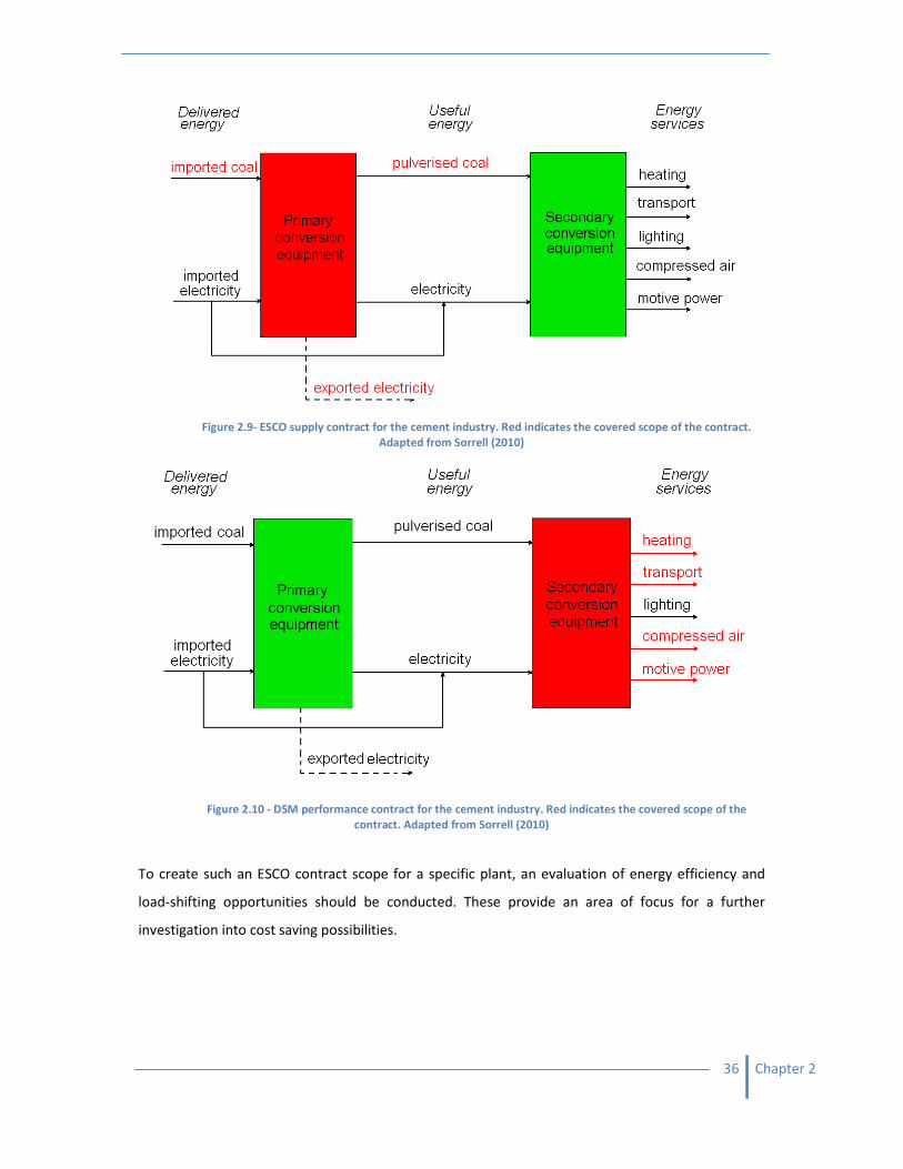
36 Chapter 2

Figure 2.9- ESCO supply contract for the cement industry. Red indicates the covered scope of the contract.

Adapted from Sorrell (2010)

Figure 2.10 - DSM performance contract for the cement industry. Red indicates the covered scope of the

contract. Adapted from Sorrell (2010)

To create such an ESCO contract scope for a specific plant, an evaluation of energy efficiency and

load-shifting opportunities should be conducted. These provide an area of focus for a further

investigation into cost saving possibilities.

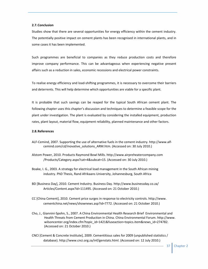
37 Chapter 2

2.7. Conclusion

Studies show that there are several opportunities for energy efficiency within the cement industry.

The potentially positive impact on cement plants has been recognised in international plants, and in

some cases it has been implemented.

Such programmes are beneficial to companies as they reduce production costs and therefore

improve company performance. This can be advantageous when experiencing negative present

affairs such as a reduction in sales, economic recessions and electrical power constraints.

To realise energy efficiency and load-shifting programmes, it is necessary to overcome their barriers

and deterrents. This will help determine which opportunities are viable for a specific plant.

It is probable that such savings can be reaped for the typical South African cement plant. The

following chapter uses this chapter’s discussion and techniques to determine a feasible scope for the

plant under investigation. The plant is evaluated by considering the installed equipment, production

rates, plant layout, material flow, equipment reliability, planned maintenance and other factors.

2.8. References

ALF-Cemind, 2007. Supporting the use of alternative fuels in the cement industry. http://www.alf-

cemind.com/cd/inovative_solutions_ARM.htm. (Accessed on: 30 July 2010.)

Alstom Power, 2010. Products Raymond Bowl Mills. http://www.airpreheatercompany.com

/Products/Category.aspx?cat=4&subcat=15. (Accessed on: 30 July 2010.)

Boake, I. G., 2003. A strategy for electrical load management in the South African mining

industry. PhD Thesis, Rand Afrikaans University, Johannesburg, South Africa

BD [Business Day], 2010. Cement Industry. Business Day. http://www.businessday.co.za/

Articles/Content.aspx?id=111495. (Accessed on: 21 October 2010.)

CC [China Cement], 2010. Cement price surges in response to electricity controls. http://www.

cementchina.net/news/shownews.asp?id=7772. (Accessed on: 21 October 2010.)

Cho, J., Giannini-Spohn, S., 2007. A China Environmental Health Research Brief Environmental and

Health Threats from Cement Production in China. China Environmental Forum. http://www.

wilsoncenter.org/index.cfm?topic_id=1421&fuseaction=topics.item&news_id=274782.

(Accessed on: 21 October 2010.)

CNCI [Cement & Concrete Institute], 2009. Cementitious sales for 2009 (unpublished statistics /

database). http://www.cnci.org.za/inf/genstats.html. (Accessed on: 12 July 2010.)

38 Chapter 2

Choate, W.T., 2003. Energy and Emission Reduction Opportunities for the Cement Industry.

BCS, Incorporated, 5550 Sterrett Place, Suite 306, Columbia, MD 21044.

Hasanbeigi, A., Menkea, C., Therdyothin, A., 2010a. The use of conservation supply curves in energy

policy and economic analysis: The case study of Thai cement industry. Energy Policy 38, 392–

405.

Hasanbeigi, A., Price, L., Lu, H., Lan, W., 2010b. Analysis of energy-efficiency opportunities for the

cement industry in Shandong Province, China: A case study of 16 cement plants. Energy 35,

3461-3473.

Hassaan, M.Y., 2001. Basalt rock as an alternative raw material in Portland cement manufacture.

Materials Letters 50, 172–178.

Holland, M. 2001. AC DC Kilns, Proc. 2001 IEEE-IAS/PCA Cement Industry Technical Conference: 75-

84, Vancouver, Canada.

Kavas, T., Olgan, A., Erdogan, Y., 2005. Setting and hardening of borogypsum–Portland cement

clinker–fly ash blends. Studies on effects of molasses on properties of mortar containing

borogypsum. Cement and Concrete Research 35, 711 –718

KEMA, 2005. Industrial Case Study: The Cement Industry, CALMAC Study ID: PGE0251.01, Final

Report. KEMA Inc., Oakland, California.

Kolip, A. 2010, Energy and exergy analyses of a serial flow four cyclone Stages precalciner type

cement plant. The University of Sakarya, Technical Education Faculty 54187, Esentepe,

Sakarya, Turkey.

LWB refractories, 2008. Cement and Lime Industry. http://www.lwbref.de/en/markets/cement-

lime-industry. (Accessed on: 30 July 2010.)

Lourens, C. 2007. Cement Sales ‘set to grow’. Business Day. http://www.businessday.co.za

/Articles/Content.aspx?id=41770. (Accessed on: 21 October 2010.)

Mokopanele, T., 2010. Infrastructure slowdown worries PPC. Business Day. http://www.businessday

.co.za/Articles/Content.aspx?id=108669. (Accessed on: 21 October 2010)

MS [Manfredini & Schianchi], 2010. Hammer mills type slammer. http://www.manfredinieschianchi.

com /301-12-2EN-hammer-mills-slammer.htm. (Accessed on: 30 July 2010.)

NSI Equipments, 2010. Ribbon Blenders & Ball Mills. http://www.nsiequipments.com/ribbon-

blenders-ball-mills.html. (Accessed on: 30 July 2010.)

PCA [Portland Cement Association], 2010. How Portland cement is made. Cement and Concrete

Basics. http://www.cement.org/basics/howmade.asp. (Accessed on: 10 June 2010.)

39 Chapter 2

Price, L., Hasanbeigi, A., Lu, H., 2009. Analysis of Energy-Efficiency Opportunities for the Cement

Industry in Shandong Province, China. Ernest Orlando Lawrence Berkeley National

Laboratory, Environmental Energy Technologies Division, Berkeley, CA, USA.

Q-filter, 2010. The encyclopedia of filters- dust collection. http://www.qfilter.com/Resource/

DocumentDetail/15. (Accessed on: November 2010.)

Regitz, J., 1996. Evaluation of Mill Drive Options IEEE Transactions on Industry Applications 3 32:

653.

Sadeghian, M., Fatehi, A., 2009. Identification of Nonlinear Predictor and Simulator Models of a

Cement Rotary Kiln by Locally Linear Neuro-Fuzzy Technique. World Academy of Science,

Engineering and Technology. http://www.waset.org/journals/waset/v58/v58-192.pdf

(Accessed on: November 2010.)

Sheen International, 2010. Clinker. http://sheeninternationalchemical.tradeindia.com/Exporters_

Suppliers/Exporter7403.95447/Clinker.html. (Accessed on: 30 July 2010.)


Tatum, M., 2010. What is Portland cement?. Wise Geek. http://www.wisegeek.com/what-is

-portland-cement.htm. (Accessed on: 22 October 2010)

Touil, D., Belaadi, S., Frances, C., 2006. Energy efficiency of cement finish grinding in a dray batch ball

mill. Cement and Concrete Research 36, 416-421.

UNIDO [United Nations Industrial Development Organisation], 1994. Output of a Seminar on Energy

Conservation in Cement Industry. P.O. Box 300, A-1400 Vienna, Austria.

Vleuten F.P. van der, 1994. Cement in Development: Energy and Environment Netherlands Energy

Research Foundation, Petten, The Netherlands.

Wansbrough, H., 2008. The Manufacture of Portland Cement. NZ Institute of Chemistry, PO

Box 39-112, Harewood, Christchurch, New Zealand.

Worrell, E., Price F.L., Powell, C., Powell, F., 2005. Case Study of the California Cement Industry.

Ernest Orlando Lawrence Berkeley National Laboratory, Environmental Energy Technologies

Division, Berkeley, CA, USA.

Worrell, E., Martin, N., Price, L., 2000. Potentials for energy efficiency improvement in the US

cement industry. Energy 25 (12), 1189-1214

Worrell, E., Galitsky, C., Price, L., 2008a. Energy Efficiency Improvement Opportunities

for the Cement Industry. Ernest Orlando Lawrence Berkeley National Laboratory,

Environmental Energy Technologies Division, Berkeley, CA, USA.

Worrell, E., Galitsky, C., Price, L., 2008b. Energy Efficiency Improvement and Cost Savings

Opportunities for Cement Making. Ernest Orlando Lawrence Berkeley National Laboratory,


40 Chapter 2

NDRC [National Development and Reform Commission], 2006. Industrial policy for the cement

industry. NDRC; Number 50 Directive, 38.S.Yuetan Street, Beijing, China.

41 Chapter 3

Chapter 3

Evaluation and simulation of a typical

South African cement plant

3.1. The cement plant under investigation

This chapter provides information on the cement plant under investigation. A completed questionnaire

and SCADA data from production lines are used to determine feasible energy efficiency opportunities

for the plant. As the particular plant represents a typical cement plant in South Africa, the same

procedure can be applied across the country to determine the energy saving possibilities.

As confidentiality of the plant will be respected, the name and location of the plant will remain

anonymous. It will therefore be referred to as the “plant under investigation” for the remainder of the

study.

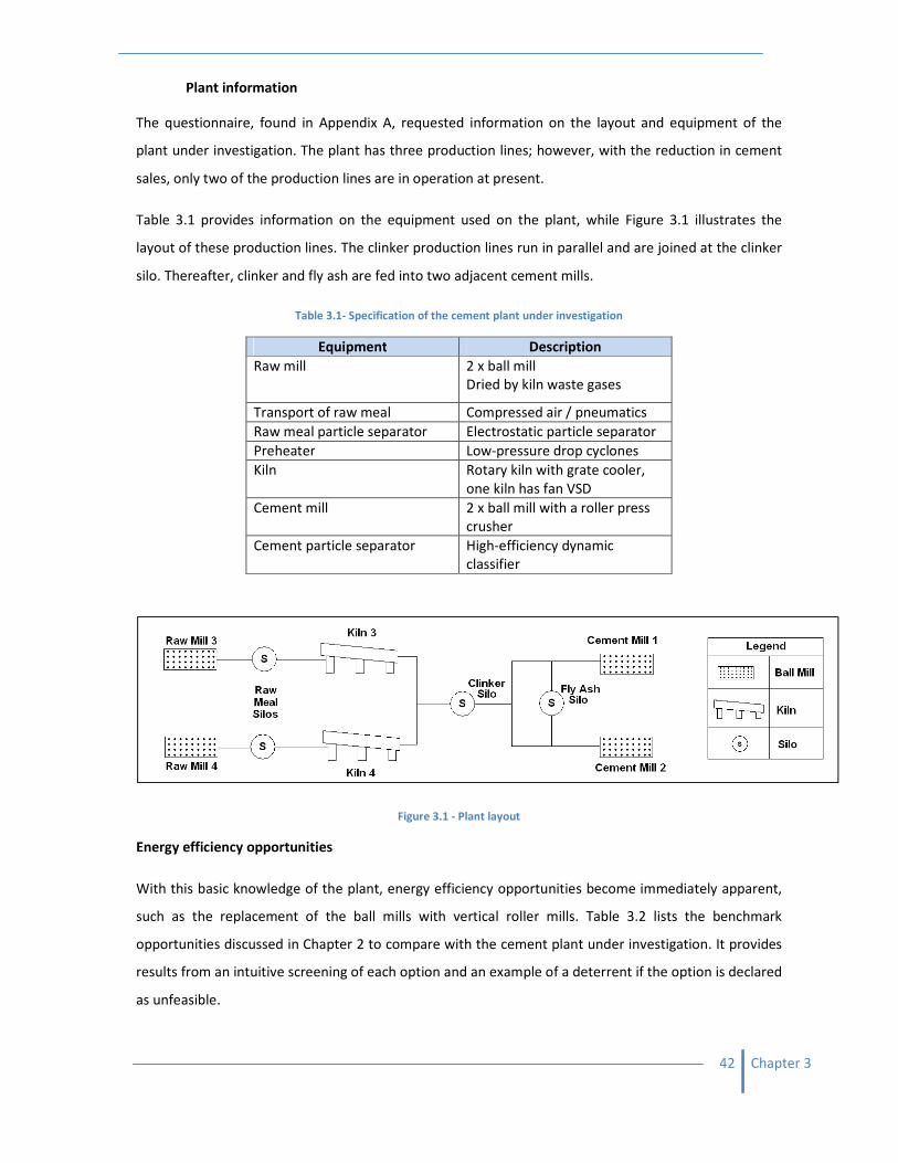
42 Chapter 3

Plant information

The questionnaire, found in Appendix A, requested information on the layout and equipment of the

plant under investigation. The plant has three production lines; however, with the reduction in cement

sales, only two of the production lines are in operation at present.

Table 3.1 provides information on the equipment used on the plant, while Figure 3.1 illustrates the

layout of these production lines. The clinker production lines run in parallel and are joined at the clinker

silo. Thereafter, clinker and fly ash are fed into two adjacent cement mills.

Table 3.1- Specification of the cement plant under investigation

Equipment Description

Raw mill 2 x ball mill

Dried by kiln waste gases

Transport of raw meal Compressed air / pneumatics

Raw meal particle separator Electrostatic particle separator

Preheater Low-pressure drop cyclones

Kiln Rotary kiln with grate cooler,

one kiln has fan VSD

Cement mill 2 x ball mill with a roller press

crusher

Cement particle separator High-efficiency dynamic

classifier

Figure 3.1 - Plant layout

Energy efficiency opportunities

With this basic knowledge of the plant, energy efficiency opportunities become immediately apparent,

such as the replacement of the ball mills with vertical roller mills. Table 3.2 lists the benchmark

opportunities discussed in Chapter 2 to compare with the cement plant under investigation. It provides

results from an intuitive screening of each option and an example of a deterrent if the option is declared

as unfeasible.

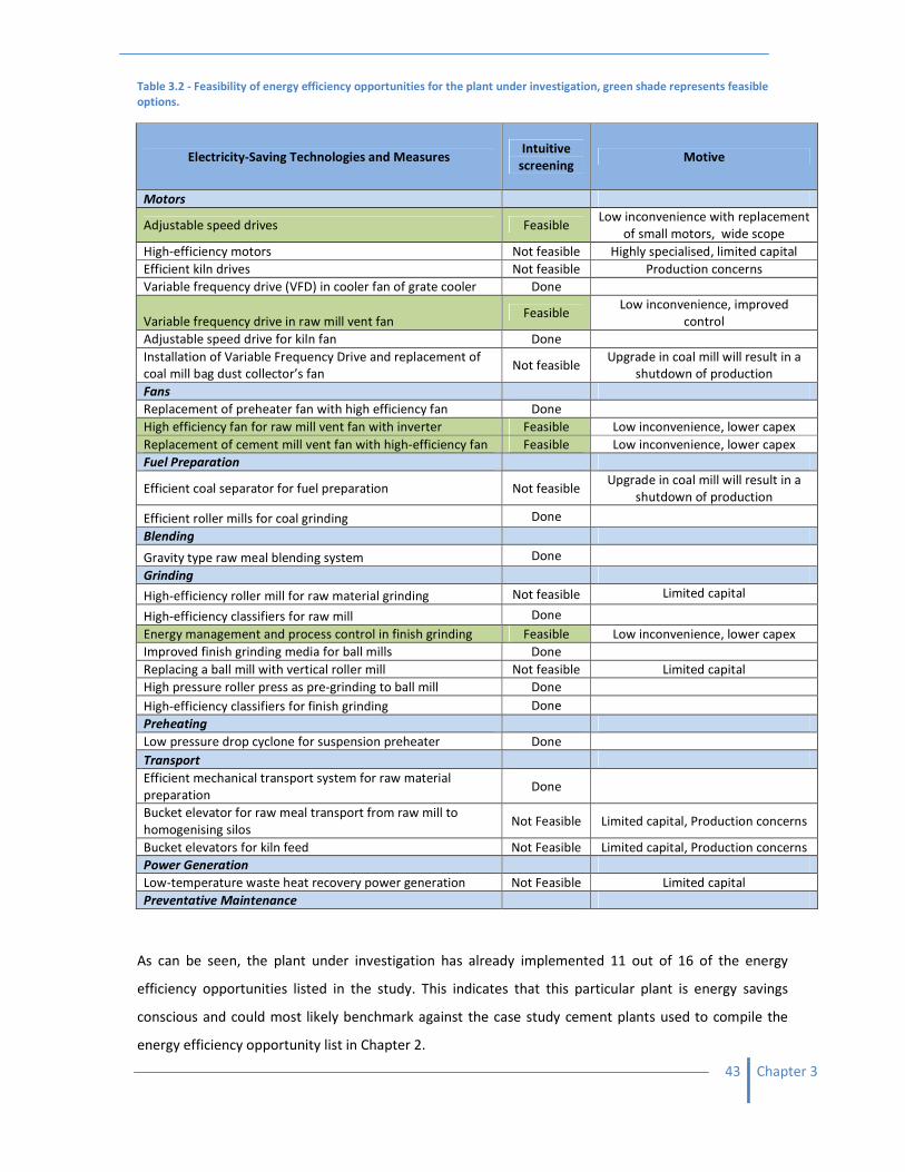
43 Chapter 3

Table 3.2 - Feasibility of energy efficiency opportunities for the plant under investigation, green shade represents feasible

options.

Electricity-Saving Technologies and Measures Intuitive

screening Motive

Motors

Adjustable speed drives Feasible Low inconvenience with replacement

of small motors, wide scope

High-efficiency motors Not feasible Highly specialised, limited capital

Efficient kiln drives Not feasible Production concerns

Variable frequency drive (VFD) in cooler fan of grate cooler Done

Variable frequency drive in raw mill vent fan Feasible

Low inconvenience, improved

control

Adjustable speed drive for kiln fan Done

Installation of Variable Frequency Drive and replacement of

coal mill bag dust collector’s fan Not feasible

Upgrade in coal mill will result in a

shutdown of production

Fans

Replacement of preheater fan with high efficiency fan Done

High efficiency fan for raw mill vent fan with inverter Feasible Low inconvenience, lower capex

Replacement of cement mill vent fan with high-efficiency fan Feasible Low inconvenience, lower capex

Fuel Preparation

Efficient coal separator for fuel preparation Not feasible Upgrade in coal mill will result in a

shutdown of production

Efficient roller mills for coal grinding Done

Blending

Gravity type raw meal blending system Done

Grinding

High-efficiency roller mill for raw material grinding Not feasible Limited capital

High-efficiency classifiers for raw mill Done

Energy management and process control in finish grinding Feasible Low inconvenience, lower capex

Improved finish grinding media for ball mills Done

Replacing a ball mill with vertical roller mill Not feasible Limited capital

High pressure roller press as pre-grinding to ball mill Done

High-efficiency classifiers for finish grinding Done

Preheating

Low pressure drop cyclone for suspension preheater Done

Transport

Efficient mechanical transport system for raw material

preparation Done

Bucket elevator for raw meal transport from raw mill to

homogenising silos Not Feasible Limited capital, Production concerns

Bucket elevators for kiln feed Not Feasible Limited capital, Production concerns

Power Generation

Low-temperature waste heat recovery power generation Not Feasible Limited capital

Preventative Maintenance

As can be seen, the plant under investigation has already implemented 11 out of 16 of the energy

efficiency opportunities listed in the study. This indicates that this particular plant is energy savings

conscious and could most likely benchmark against the case study cement plants used to compile the

energy efficiency opportunity list in Chapter 2.

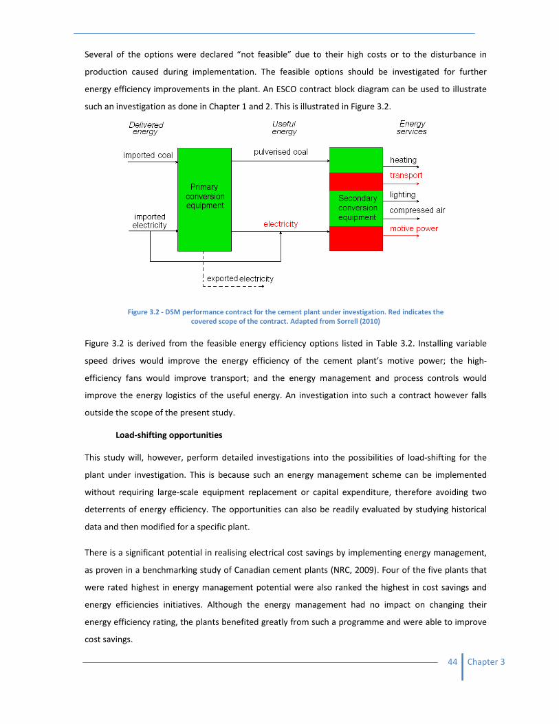
44 Chapter 3

Several of the options were declared “not feasible” due to their high costs or to the disturbance in

production caused during implementation. The feasible options should be investigated for further

energy efficiency improvements in the plant. An ESCO contract block diagram can be used to illustrate

such an investigation as done in Chapter 1 and 2. This is illustrated in Figure 3.2.

Figure 3.2 - DSM performance contract for the cement plant under investigation. Red indicates the

covered scope of the contract. Adapted from Sorrell (2010)

Figure 3.2 is derived from the feasible energy efficiency options listed in Table 3.2. Installing variable

speed drives would improve the energy efficiency of the cement plant’s motive power; the high-

efficiency fans would improve transport; and the energy management and process controls would

improve the energy logistics of the useful energy. An investigation into such a contract however falls

outside the scope of the present study.

Load-shifting opportunities

This study will, however, perform detailed investigations into the possibilities of load-shifting for the

plant under investigation. This is because such an energy management scheme can be implemented

without requiring large-scale equipment replacement or capital expenditure, therefore avoiding two

deterrents of energy efficiency. The opportunities can also be readily evaluated by studying historical

data and then modified for a specific plant.

There is a significant potential in realising electrical cost savings by implementing energy management,

as proven in a benchmarking study of Canadian cement plants (NRC, 2009). Four of the five plants that

were rated highest in energy management potential were also ranked the highest in cost savings and

energy efficiencies initiatives. Although the energy management had no impact on changing their

energy efficiency rating, the plants benefited greatly from such a programme and were able to improve

cost savings.

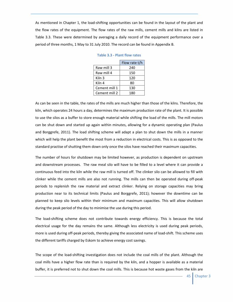
45 Chapter 3

As mentioned in Chapter 1, the load-shifting opportunities can be found in the layout of the plant and

the flow rates of the equipment. The flow rates of the raw mills, cement mills and kilns are listed in

Table 3.3. These were determined by averaging a daily record of the equipment performance over a

period of three months, 1 May to 31 July 2010. The record can be found in Appendix B.

Table 3.3 - Plant flow rates

As can be seen in the table, the rates of the mills are much higher than those of the kilns. Therefore, the

kiln, which operates 24 hours a day, determines the maximum production rate of the plant. It is possible

to use the silos as a buffer to store enough material while shifting the load of the mills. The mill motors

can be shut down and started up again within minutes, allowing for a dynamic operating plan (Paulus

and Borggrefe, 2011). The load shifting scheme will adapt a plan to shut down the mills in a manner

which will help the plant benefit the most from a reduction in electrical costs. This is as opposed to the

standard practise of shutting them down only once the silos have reached their maximum capacities.

The number of hours for shutdown may be limited however, as production is dependent on upstream

and downstream processes. The raw meal silo will have to be filled to a level where it can provide a

continuous feed into the kiln while the raw mill is turned off. The clinker silo can be allowed to fill with

clinker while the cement mills are also not running. The mills can then be operated during off-peak

periods to replenish the raw material and extract clinker. Relying on storage capacities may bring

production near to its technical limits (Paulus and Borggrefe, 2011); however the downtime can be

planned to keep silo levels within their minimum and maximum capacities. This will allow shutdown

during the peak period of the day to minimise the use during this period.

The load-shifting scheme does not contribute towards energy efficiency. This is because the total

electrical usage for the day remains the same. Although less electricity is used during peak periods,

more is used during off-peak periods, thereby giving the associated name of load-shift. This scheme uses

the different tariffs charged by Eskom to achieve energy cost savings.

The scope of the load-shifting investigation does not include the coal mills of the plant. Although the

coal mills have a higher flow rate than is required by the kiln, and a hopper is available as a material

buffer, it is preferred not to shut down the coal mills. This is because hot waste gases from the kiln are

Flow rate t/h

Raw mill 3 240

Raw mill 4 150

Kiln 3 120

Kiln 4 80

Cement mill 1 130

Cement mill 2 180

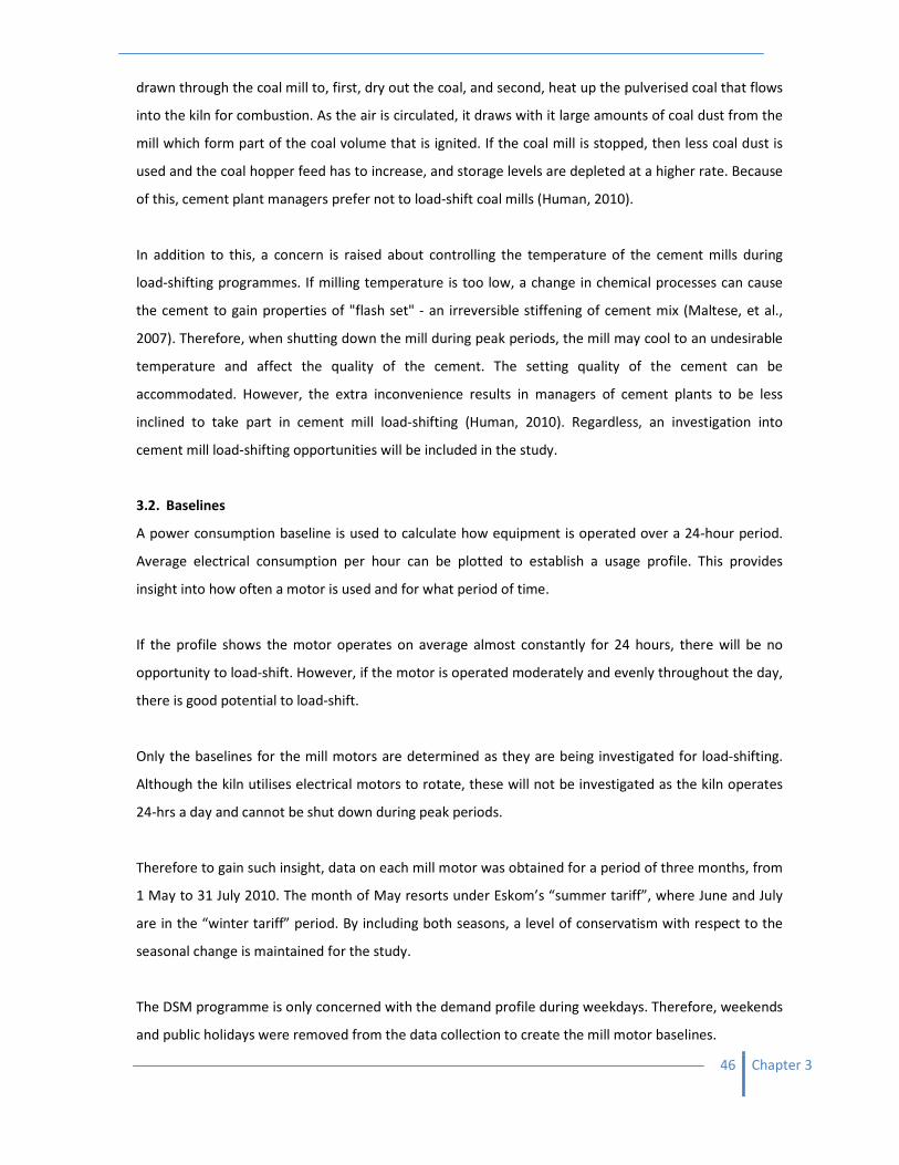
46 Chapter 3

drawn through the coal mill to, first, dry out the coal, and second, heat up the pulverised coal that flows

into the kiln for combustion. As the air is circulated, it draws with it large amounts of coal dust from the

mill which form part of the coal volume that is ignited. If the coal mill is stopped, then less coal dust is

used and the coal hopper feed has to increase, and storage levels are depleted at a higher rate. Because

of this, cement plant managers prefer not to load-shift coal mills (Human, 2010).

In addition to this, a concern is raised about controlling the temperature of the cement mills during

load-shifting programmes. If milling temperature is too low, a change in chemical processes can cause

the cement to gain properties of "flash set" - an irreversible stiffening of cement mix (Maltese, et al.,

2007). Therefore, when shutting down the mill during peak periods, the mill may cool to an undesirable

temperature and affect the quality of the cement. The setting quality of the cement can be

accommodated. However, the extra inconvenience results in managers of cement plants to be less

inclined to take part in cement mill load-shifting (Human, 2010). Regardless, an investigation into

cement mill load-shifting opportunities will be included in the study.

3.2. Baselines

A power consumption baseline is used to calculate how equipment is operated over a 24-hour period.

Average electrical consumption per hour can be plotted to establish a usage profile. This provides

insight into how often a motor is used and for what period of time.

If the profile shows the motor operates on average almost constantly for 24 hours, there will be no

opportunity to load-shift. However, if the motor is operated moderately and evenly throughout the day,

there is good potential to load-shift.

Only the baselines for the mill motors are determined as they are being investigated for load-shifting.

Although the kiln utilises electrical motors to rotate, these will not be investigated as the kiln operates

24-hrs a day and cannot be shut down during peak periods.

Therefore to gain such insight, data on each mill motor was obtained for a period of three months, from

1 May to 31 July 2010. The month of May resorts under Eskom’s “summer tariff”, where June and July

are in the “winter tariff” period. By including both seasons, a level of conservatism with respect to the

seasonal change is maintained for the study.

The DSM programme is only concerned with the demand profile during weekdays. Therefore, weekends

and public holidays were removed from the data collection to create the mill motor baselines.

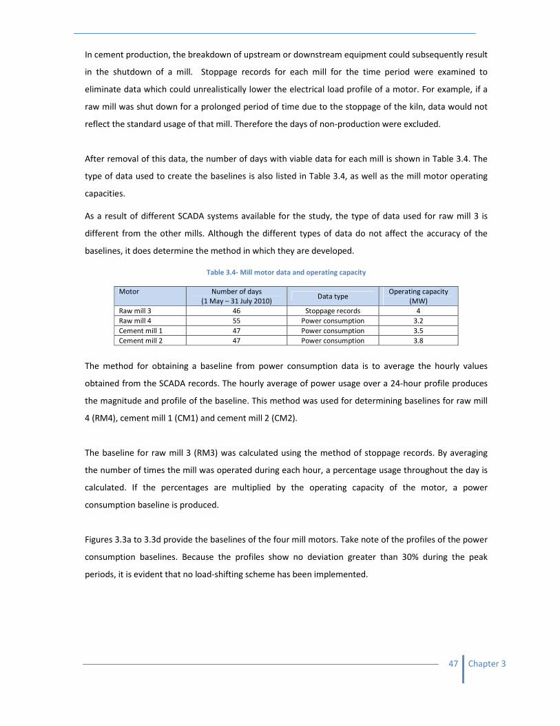
47 Chapter 3

In cement production, the breakdown of upstream or downstream equipment could subsequently result

in the shutdown of a mill. Stoppage records for each mill for the time period were examined to

eliminate data which could unrealistically lower the electrical load profile of a motor. For example, if a

raw mill was shut down for a prolonged period of time due to the stoppage of the kiln, data would not

reflect the standard usage of that mill. Therefore the days of non-production were excluded.

After removal of this data, the number of days with viable data for each mill is shown in Table 3.4. The

type of data used to create the baselines is also listed in Table 3.4, as well as the mill motor operating

capacities.

As a result of different SCADA systems available for the study, the type of data used for raw mill 3 is

different from the other mills. Although the different types of data do not affect the accuracy of the

baselines, it does determine the method in which they are developed.

Table 3.4- Mill motor data and operating capacity

The method for obtaining a baseline from power consumption data is to average the hourly values

obtained from the SCADA records. The hourly average of power usage over a 24-hour profile produces

the magnitude and profile of the baseline. This method was used for determining baselines for raw mill

4 (RM4), cement mill 1 (CM1) and cement mill 2 (CM2).

The baseline for raw mill 3 (RM3) was calculated using the method of stoppage records. By averaging

the number of times the mill was operated during each hour, a percentage usage throughout the day is

calculated. If the percentages are multiplied by the operating capacity of the motor, a power

consumption baseline is produced.

Figures 3.3a to 3.3d provide the baselines of the four mill motors. Take note of the profiles of the power

consumption baselines. Because the profiles show no deviation greater than 30% during the peak

periods, it is evident that no load-shifting scheme has been implemented.

Motor Number of days

(1 May – 31 July 2010) Data type

Operating capacity

(MW)

Raw mill 3 46 Stoppage records 4

Raw mill 4 55 Power consumption 3.2

Cement mill 1 47 Power consumption 3.5

Cement mill 2 47 Power consumption 3.8

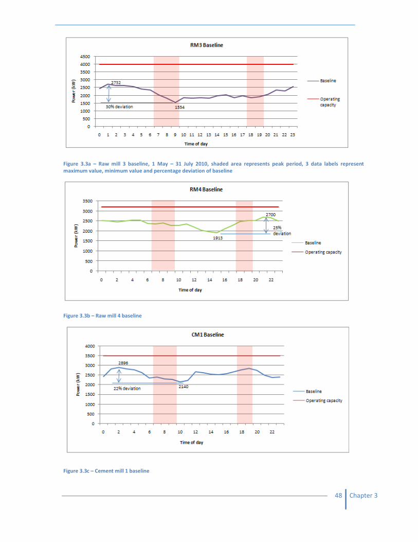
48 Chapter 3

Figure 3.3a – Raw mill 3 baseline, 1 May – 31 July 2010, shaded area represents peak period, 3 data labels represent

maximum value, minimum value and percentage deviation of baseline

Figure 3.3b – Raw mill 4 baseline

Figure 3.3c – Cement mill 1 baseline

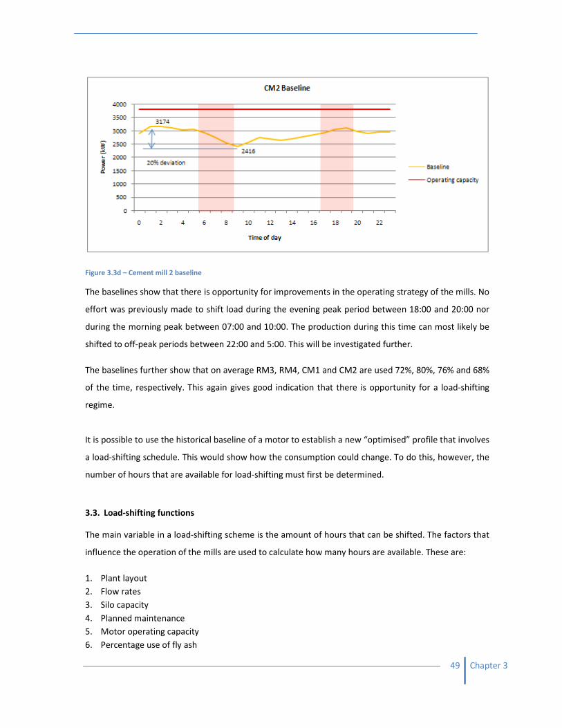
49 Chapter 3

Figure 3.3d – Cement mill 2 baseline

The baselines show that there is opportunity for improvements in the operating strategy of the mills. No

effort was previously made to shift load during the evening peak period between 18:00 and 20:00 nor

during the morning peak between 07:00 and 10:00. The production during this time can most likely be

shifted to off-peak periods between 22:00 and 5:00. This will be investigated further.

The baselines further show that on average RM3, RM4, CM1 and CM2 are used 72%, 80%, 76% and 68%

of the time, respectively. This again gives good indication that there is opportunity for a load-shifting

regime.

It is possible to use the historical baseline of a motor to establish a new “optimised” profile that involves

a load-shifting schedule. This would show how the consumption could change. To do this, however, the

number of hours that are available for load-shifting must first be determined.

3.3. Load-shifting functions

The main variable in a load-shifting scheme is the amount of hours that can be shifted. The factors that

influence the operation of the mills are used to calculate how many hours are available. These are:

1. Plant layout

2. Flow rates

3. Silo capacity

4. Planned maintenance

5. Motor operating capacity

6. Percentage use of fly ash

50 Chapter 3

7. Equipment reliability (incident hours)

8. Regulations of DSM load-shifting

9. Weekend operating hours

A simulation can be used to determine how many hours are available for the load-shifting of equipment

feeding into or out of a silo. Flow rates, percentage fly ash and reliability are factors that are variable.

The simulation can be used in different scenarios to calculate how many load-shifting hours are

available as the factors change.

Silo Simulation

The number of hours load-shifted, directly affects the operating hours (OH) of equipment preceding and

following the silo. OH is the dominant variable that influences the change in silo level. This is because it

determines the amount of material flowing into and out of the silo. The changes in silo level may be

calculated by multiplying the flow rates of equipment with the operating hours of the day as can be

seen in Equation 1:

– Eq. 1

The major constraint for the simulation is that the silo level has to stay within the capacity range for a

specified duration of time. The range is defined as the array between maximum silo capacity and

minimum silo capacity, as illustrated in Figure 3.4.

The simulation calculates available shut-down time of equipment for 31 days. The load-shifting hours

are determined for either the inflow material or the outflow material depending on which silo is being

simulated; either the raw meal silo or the clinker silo. The simulations for the silos differ slightly and will

therefore be discussed separately.

Figure 3.4 - Silo Specifications

51 Chapter 3

Raw Meal Silo

Figure 3.5 illustrates the equipment involved in the raw meal silo simulation. Since the kiln needs to

operate 24 hours a day, load-shifting is only calculated for the raw mill in the raw meal silo simulation.

This determines how much material is fed into the silo. Therefore the simulation needs to calculate how

many hours are available for load-shifting without the raw meal silo reducing beyond minimum capacity.

Figure 3.5 - Raw meal silo

To do this, the following information needs to be obtained: operating hours of equipment, flow rates,

actual silo level, planned maintenance, and equipment reliability.

The simulation begins by using data from SCADA readings from three sources: 1) the silo, 2) the raw mill

and 3) the kiln.

1) The silo SCADA provides the actual silo level. This gives a starting point from which to run the

simulation of changing silo level.

2) The raw mill SCADA provides a) the inflow rate of material into the silo and b) the recent

reliability factor for the mill.

a. The flow rate value is calculated by averaging the flow rate readings for the previous week.

This considers the recent performance of the mill.

b. The reliability factor of the mill is expressed as average daily incident hours over the last

month.

3) The SCADA data from the mill would also provide a) outflow rate and b) average incident hours.

a. The flow rate out of the silo is again calculated from the average readings for the previous

week. The values averaged may be either the rate of material fed into the kiln, or the rate at

which clinker is produced by the kiln while taking into consideration the percentage weight-

loss during the sintering process.

b. Incident hours will again express the reliability of the kiln. However, it is acceptable to

assume the kiln incident hours are equal to zero. This is because the kiln usually operates

24-hours a day if the production line is functioning.

52 Chapter 3

The simulation takes into account the reliability factor of the mills by subtracting incident hours from

the daily OH. The incident hours are dependent on the reliability of not only the mills, but also the

auxiliary equipment and the equipment of upstream and downstream processes. The incident hours

used in the daily OH calculation differ on a daily basis. This is because the simulation programme

randomly generates numbers per day that are within a range around the historical average.

The range is determined from the standard deviation of the historical incident hours. For the plant

under investigation, a range of 30% was used. This is because the standard deviation of the incident

hours in the historic data equals to 27% and was rounded up for conservatism. The chances of the

simulation providing unrealistic results are reduced by influencing the daily OH with changing incident

hours. Then the probability of the silo level leaving the capacity range can be calculated.

OH is further affected by planned stoppages for the maintenance of equipment. Planned maintenance

occurs on a regular basis and can be put into the simulation as an unchanging characteristic.

Maintenance is performed for a certain amount of hours, on a specific day of the week, for a number of

times during the month. The simulation keeps track of time and date to consider planned stoppages in

the future. The OH on a day of maintenance would be calculated as 24 hours minus the incident hours,

load-shifting and maintenance hours as seen in Equation 2.

�� 24 – �� – �� – �� )*. 2

The simulation can vary the load-shifting hours of the raw mill to alter the OH. This will result in

predicting how silo levels will change as incident hours vary. Because of the large increments between

full-load-shifting hours, the change in the simulation from one amount to another is significant. It can

therefore be easily seen if the mill load can be shifted for, for instance, two or three hours. This is while

taking into consideration the present production and performance. The maximum available load-shifting

hours are later used for calculating an optimised baseline.

Figure 3.6 provides a flow diagram of the factors involved in the simulation as discussed above. Table

3.5 and Figure 3.7 show the salient calculations of the simulation and the resulting silo level graph for a

period of a month. Appendix C provides a further description of the simulation.

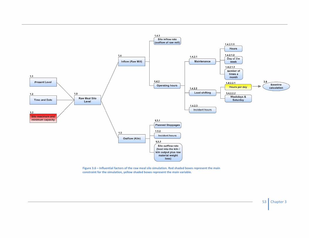
53 Chapter 3

Figure 3.6 – Influential factors of the raw meal silo simulation. Red shaded boxes represent the main

constraint for the simulation, yellow shaded boxes represent the main variable.

54 Chapter 3

Table 3.5 - Raw meal silo simulation calculations

Raw Mill 3

Kiln 3

Silo (t)

Silo (t) D

ay

Inci

de

nt

(h)

Ma

inte

na

nce

(h)

Loa

d-s

hif

t (h

)

OH

(h

)

Ou

tpu

t (t

)

OH

(h

)

Ou

tpu

t (t

)

sta

rt

12000

Max capacity 16000 1 6.04 6 11.96 2811 ## 21.67 2600 12210

Starting level (%) 80

2 6.87

6 11.13 2616 ## 24.00 2880

11947

Min level 10000

3 5.54

6 12.46 2929 ## 24.00 2880

11995

4 4.50

6 13.50 3172 ## 21.76 2612

12555

5 5.04

6 12.96 3045 ## 24.00 2880

12720

Flow rate (t/h)

6 4.12

0 15.88 3731 ## 24.00 2880

13572

RM3 output (t/h) 235

7 7.24

0 12.76 2998 ## 22.64 2717

13853

Kiln3 input (t/h) 120 1 5.35 6 12.65 2974 ## 22.33 2679 14148

2 6.67 9 6 2.33 547 ## 21.16 2540

12155

3 4.85

6 13.15 3089 ## 24.00 2880

12365

4 7.77

6 10.23 2404 ## 24.00 2880

11888

Load-shift (h) 6 5 6.26 6 11.74 2759 ## 22.14 2657 11990

Weekend OH 20

6 5.55

0 14.45 3396 ## 19.66 2359

13027

Incident (h) 7 7.90 0 12.10 2843 ## 22.04 2645 13225

Raw mill 3 Kiln 3 1 4.80 6 13.20 3101 ## 24.00 2880 13446

5.6 1.23

2 6.04

6 11.96 2810 ## 24.00 2880

13376

3 5.59

6 12.41 2916 ## 20.55 2466

13826

4 6.86

6 11.14 2617 ## 24.00 2880

13563

5 6.35

6 11.65 2737 ## 24.00 2880

13420

6 5.99 0 14.01 3292 ## 24.00 2880 13832

7 7.29

0 12.71 2986 ## 23.37 2805

14014

1 5.31

6 12.69 2981 ## 19.03 2284

14711

2 4.91 9 6 4.09 962 ## 21.40 2568

13105

3 7.48

6 10.52 2472 ## 20.12 2414

13163

4 4.57

6 13.43 3156 ## 24.00 2880

13439

5 7.03

6 10.97 2577 ## 21.64 2597

13419

6 6.09 0 13.91 3268 ## 23.98 2877 13810

7 4.56

0 15.44 3629 ## 24.00 2880

14559

1 5.10

6 12.90 3031 ## 21.18 2541

15049

2 7.01

6 10.99 2584 ## 20.30 2436

15197

3 5.86

6 12.14 2852 ## 24.00 2880

15169

Figure 3.7- Change in raw meal silo level

9500

10500

11500

12500

13500

14500

15500

16500

1 3 5 7 9 11 13 15 17 19 21 23 25 27 29 31

Sil

o c

ap

aci

ty (

t)

Days of the month

Raw mill 3 silo level

Silo level

Maximum

capacity

Minimum

capacity

Incident hours – Randomly generated numbers between 30% brackets of average incident hours of the mill

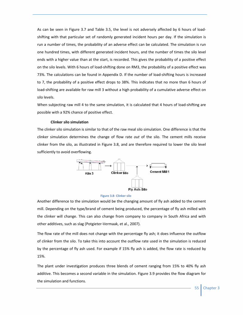
55 Chapter 3

As can be seen in Figure 3.7 and Table 3.5, the level is not adversely affected by 6 hours of load-

shifting with that particular set of randomly generated incident hours per day. If the simulation is

run a number of times, the probability of an adverse effect can be calculated. The simulation is run

one hundred times, with different generated incident hours, and the number of times the silo level

ends with a higher value than at the start, is recorded. This gives the probability of a positive effect

on the silo levels. With 6 hours of load-shifting done on RM3, the probability of a positive effect was

73%. The calculations can be found in Appendix D. If the number of load-shifting hours is increased

to 7, the probability of a positive effect drops to 38%. This indicates that no more than 6 hours of

load-shifting are available for raw mill 3 without a high probability of a cumulative adverse effect on

silo levels.

When subjecting raw mill 4 to the same simulation, it is calculated that 4 hours of load-shifting are

possible with a 92% chance of positive effect.

Clinker silo simulation

The clinker silo simulation is similar to that of the raw meal silo simulation. One difference is that the

clinker simulation determines the change of flow rate out of the silo. The cement mills receive

clinker from the silo, as illustrated in Figure 3.8, and are therefore required to lower the silo level

sufficiently to avoid overflowing.

Another difference to the simulation would be the changing amount of fly ash added to the cement

mill. Depending on the type/brand of cement being produced, the percentage of fly ash milled with

the clinker will change. This can also change from company to company in South Africa and with

other additives, such as slag (Potgieter-Vermaak, et al., 2007).

The flow rate of the mill does not change with the percentage fly ash; it does influence the outflow

of clinker from the silo. To take this into account the outflow rate used in the simulation is reduced

by the percentage of fly ash used. For example if 15% fly ash is added, the flow rate is reduced by

15%.

The plant under investigation produces three blends of cement ranging from 15% to 40% fly ash

additive. This becomes a second variable in the simulation. Figure 3.9 provides the flow diagram for

the simulation and functions.

Figure 3.8- Clinker silo

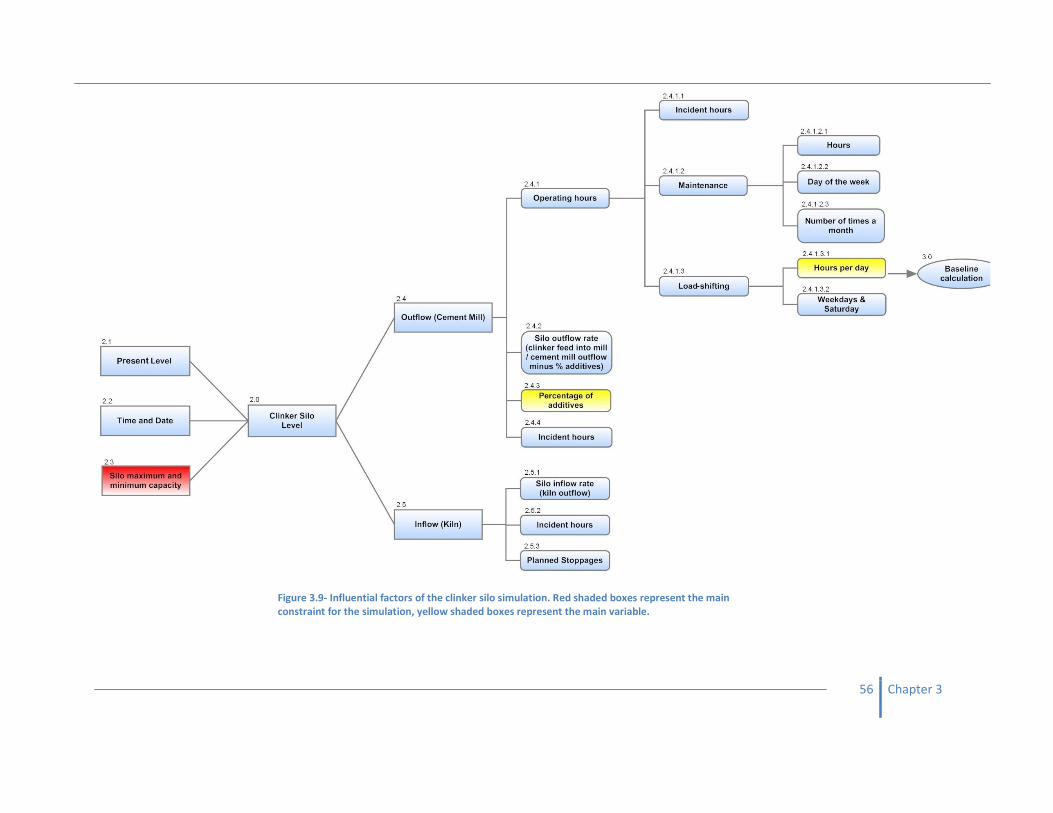
56 Chapter 3

Figure 3.9- Influential factors of the clinker silo simulation. Red shaded boxes represent the main

constraint for the simulation, yellow shaded boxes represent the main variable.

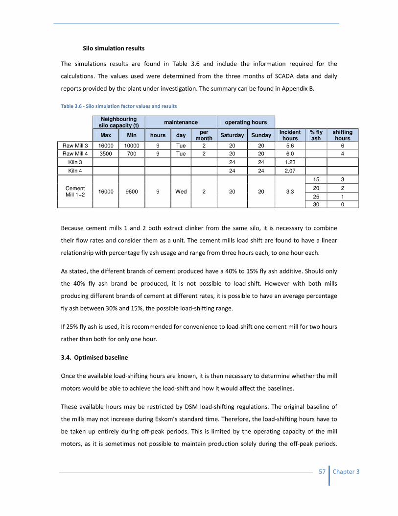
57 Chapter 3

Silo simulation results

The simulations results are found in Table 3.6 and include the information required for the

calculations. The values used were determined from the three months of SCADA data and daily

reports provided by the plant under investigation. The summary can be found in Appendix B.

Table 3.6 - Silo simulation factor values and results

Neighbouring silo capacity (t)

maintenance operating hours

Max Min hours day

per month

Saturday Sunday Incident hours

% fly ash

shifting hours

Raw Mill 3 16000 10000 9 Tue 2 20 20 5.6

6

Raw Mill 4 3500 700 9 Tue 2 20 20 6.0

4

Kiln 3

24 24 1.23

Kiln 4

24 24 2.07

Cement

Mill 1+2 16000 9600 9 Wed 2 20 20 3.3

15 3

20 2

25 1

30 0

Because cement mills 1 and 2 both extract clinker from the same silo, it is necessary to combine

their flow rates and consider them as a unit. The cement mills load shift are found to have a linear

relationship with percentage fly ash usage and range from three hours each, to one hour each.

As stated, the different brands of cement produced have a 40% to 15% fly ash additive. Should only

the 40% fly ash brand be produced, it is not possible to load-shift. However with both mills

producing different brands of cement at different rates, it is possible to have an average percentage

fly ash between 30% and 15%, the possible load-shifting range.

If 25% fly ash is used, it is recommended for convenience to load-shift one cement mill for two hours

rather than both for only one hour.

3.4. Optimised baseline

Once the available load-shifting hours are known, it is then necessary to determine whether the mill

motors would be able to achieve the load-shift and how it would affect the baselines.

These available hours may be restricted by DSM load-shifting regulations. The original baseline of

the mills may not increase during Eskom’s standard time. Therefore, the load-shifting hours have to

be taken up entirely during off-peak periods. This is limited by the operating capacity of the mill

motors, as it is sometimes not possible to maintain production solely during the off-peak periods.

58 Chapter 3

The degree to which the available hours are limited can be determined by optimising baseline

profiles to remain below operating capacity.

Another simulation is used to determine the best possible load-shifting strategy without exceeding

motor installed capacity or raising the standard time usage. The simulation calculates an updated

baseline for the preceding 31 day range. This is to determine how performance compares to the

original baseline.

If the standard time values of the updated baseline are not above the original values, load may be

shifted from peak periods. If not, an amount of load-shifting would also have to occur during

standard time for the following days to lower the baseline.

The new baseline must have the same total area under the curve (AUC). This is because the AUC

indicates how often the mill motors are run and therefore, the production of the mill. If the AUC is

lowered, the production will be adversely affected.

The new baseline consists of the original baseline with two changes:

1) A number of peak period hours are equated to zero. These are the load-shifted hours. The

maximum number of hours is calculated by the previous silo simulations;

2) The off-peak usage is increased to insure the AUC is not reduced during the load-shifting

scheme.

If the off-peak values are higher than the operating capacity of the mill motors, then the baseline is

not achievable and less load-shifting hours need to be implemented. The new off-peak power

consumption should be marginally, say 2%, lower than the operating capacity of the motors to allow

for unplanned breakages. With a 2% margin, an extra 14.4 hours of unplanned breakages can occur

during off-peak periods without affecting production.

With the above logic an optimised baseline is developed. Figure 3.10 provides the flow diagram for

the optimised baseline simulation.

59 Chapter 3

Figure 3.10 – Optimised baseline simulation. Red shaded boxes represent the

main constraint for the simulation, yellow shaded boxes represent the main

variable and black shaded boxes show tariff times periods.

60 Chapter 3

Figures 3.11a to 3.11c present the achievable load-shifting profiles for the mills calculated by the

baseline simulation.

Figure 3.11a - Raw mill 3 optimised profile

Figure 3.11b - Raw mill 4 optimised profile

0

500

1000

1500

2000

2500

3000

3500

4000

4500

0 1 2 3 4 5 6 7 8 9 10 11 12 13 14 15 16 17 18 19 20 21 22 23

Po

we

r (k

W)

Time of day

Raw Mill 3 Optimised Profile

Actual Baseline

Optimise Baseline

0

500

1000

1500

2000

2500

3000

3500

0 1 2 3 4 5 6 7 8 9 10 11 12 13 14 15 16 17 18 19 20 21 22 23

Po

we

r (k

W)

Time of day

Raw Mill 4 Optimised Profile

Actual Baseline

Optimise Baseline

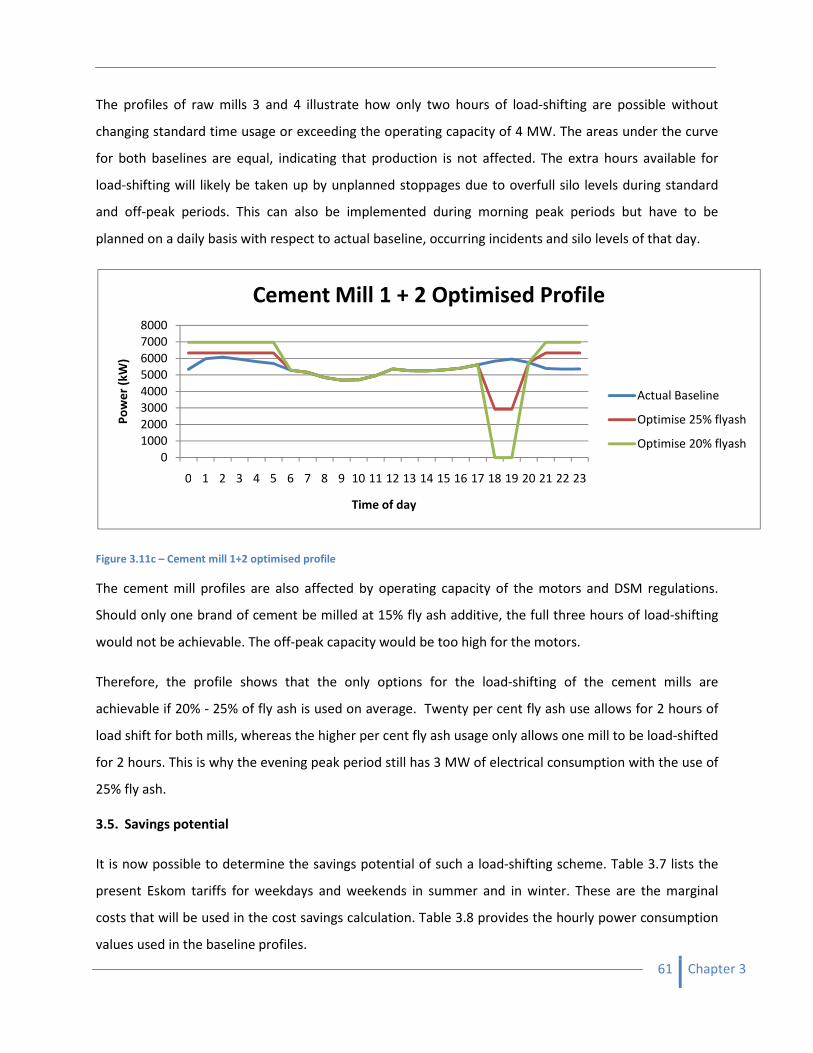
61 Chapter 3

The profiles of raw mills 3 and 4 illustrate how only two hours of load-shifting are possible without

changing standard time usage or exceeding the operating capacity of 4 MW. The areas under the curve

for both baselines are equal, indicating that production is not affected. The extra hours available for

load-shifting will likely be taken up by unplanned stoppages due to overfull silo levels during standard

and off-peak periods. This can also be implemented during morning peak periods but have to be

planned on a daily basis with respect to actual baseline, occurring incidents and silo levels of that day.

Figure 3.11c – Cement mill 1+2 optimised profile

The cement mill profiles are also affected by operating capacity of the motors and DSM regulations.

Should only one brand of cement be milled at 15% fly ash additive, the full three hours of load-shifting

would not be achievable. The off-peak capacity would be too high for the motors.

Therefore, the profile shows that the only options for the load-shifting of the cement mills are

achievable if 20% - 25% of fly ash is used on average. Twenty per cent fly ash use allows for 2 hours of

load shift for both mills, whereas the higher per cent fly ash usage only allows one mill to be load-shifted

for 2 hours. This is why the evening peak period still has 3 MW of electrical consumption with the use of

25% fly ash.

3.5. Savings potential

It is now possible to determine the savings potential of such a load-shifting scheme. Table 3.7 lists the

present Eskom tariffs for weekdays and weekends in summer and in winter. These are the marginal

costs that will be used in the cost savings calculation. Table 3.8 provides the hourly power consumption

values used in the baseline profiles.

0

1000

2000

3000

4000

5000

6000

7000

8000

0 1 2 3 4 5 6 7 8 9 10 11 12 13 14 15 16 17 18 19 20 21 22 23

Po

we

r (k

W)

Time of day

Cement Mill 1 + 2 Optimised Profile

Actual Baseline

Optimise 25% flyash

Optimise 20% flyash

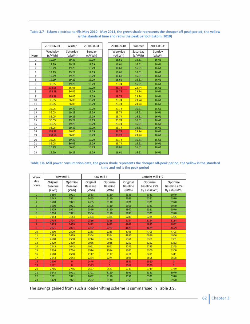
62 Chapter 3

Table 3.7 - Eskom electrical tariffs May 2010 - May 2011, the green shade represents the cheaper off-peak period, the yellow

is the standard time and red is the peak period (Eskom, 2010)

2010-06-01 Winter 2010-08-31

2010-09-01 Summer 2011-05-31

Hour

Weekday

(c/kWh)

Saturday

(c/kWh)

Sunday

(c/kWh)

Weekday

(c/kWh)

Saturday

(c/kWh)

Sunday

(c/kWh)

0 19.29 19.29 19.29 16.61 16.61 16.61

1 19.29 19.29 19.29 16.61 16.61 16.61

2 19.29 19.29 19.29 16.61 16.61 16.61

3 19.29 19.29 19.29 16.61 16.61 16.61

4 19.29 19.29 19.29 16.61 16.61 16.61

5 19.29 19.29 19.29 16.61 16.61 16.61

6 36.05 19.29 19.29 23.74 16.61 16.61

7 138.58 36.05 19.29 38.73 23.74 16.61

8 138.58 36.05 19.29 38.73 23.74 16.61

9 138.58 36.05 19.29 38.73 23.74 16.61

10 36.05 36.05 19.29 23.74 23.74 16.61

11 36.05 36.05 19.29 23.74 23.74 16.61

12 36.05 19.29 19.29 23.74 16.61 16.61

13 36.05 19.29 19.29 23.74 16.61 16.61

14 36.05 19.29 19.29 23.74 16.61 16.61

15 36.05 19.29 19.29 23.74 16.61 16.61

16 36.05 19.29 19.29 23.74 16.61 16.61

17 36.05 19.29 19.29 23.74 16.61 16.61

18 138.58 36.05 19.29 38.73 23.74 16.61

19 138.58 36.05 19.29 38.73 23.74 16.61

20 36.05 19.29 19.29 23.74 16.61 16.61

21 36.05 36.05 19.29 23.74 16.61 16.61

22 19.29 36.05 19.29 16.61 16.61 16.61

23 19.29 19.29 19.29 16.61 16.61 16.61

Table 3.8- Mill power consumption data, the green shade represents the cheaper off-peak period, the yellow is the standard

time and red is the peak period

Week

day

hours

Raw mill 3 Raw mill 4 Cement mill 1+2

Original

Baseline

(kWh)

Optimise

Baseline

(kWh)

Original

Baseline

(kWh)

Optimise

Baseline

(kWh)

Original

Baseline

(kWh)

Optimise

Baseline 25%

fly ash (kWh)

Optimise

Baseline 20%

fly ash (kWh)

0 3286 3921 2533 3110 5336 6321 6970

1 3643 3921 2495 3110 5982 6321 6970

2 3500 3921 2455 3110 6071 6321 6970

3 3500 3921 2506 3110 5951 6321 6970

4 3429 3921 2556 3110 5800 6321 6970

5 3214 3921 2564 3110 5690 6321 6970

6 3143 3143 2384 2384 5285 5285 5285

7 2714 2714 2366 2366 5154 5154 5154

8 2429 2429 2412 2412 4842 4842 4842

9 2071 2071 2287 2287 4679 4679 4679

10 2500 2500 2283 2283 4703 4703 4703

11 2429 2429 2354 2354 4956 4956 4956

12 2500 2500 2214 2214 5361 5361 5361

13 2429 2429 2036 2036 5252 5252 5252

14 2643 2643 1961 1961 5245 5245 5245

15 2714 2714 1914 1914 5300 5300 5300

16 2500 2500 2117 2117 5411 5411 5411

17 2643 2643 2274 2274 5608 5608 5608

18 2500 0 2470 0 5833 2920 0

19 2571 0 2523 0 5962 2920 0

20 2786 2786 2527 2527 5749 5749 5749

21 3143 3921 2701 3110 5391 6321 6970

22 3071 3921 2682 3110 5351 6321 6970

23 3429 3921 2502 3110 5359 6321 6970

The savings gained from such a load-shifting scheme is summarised in Table 3.9.

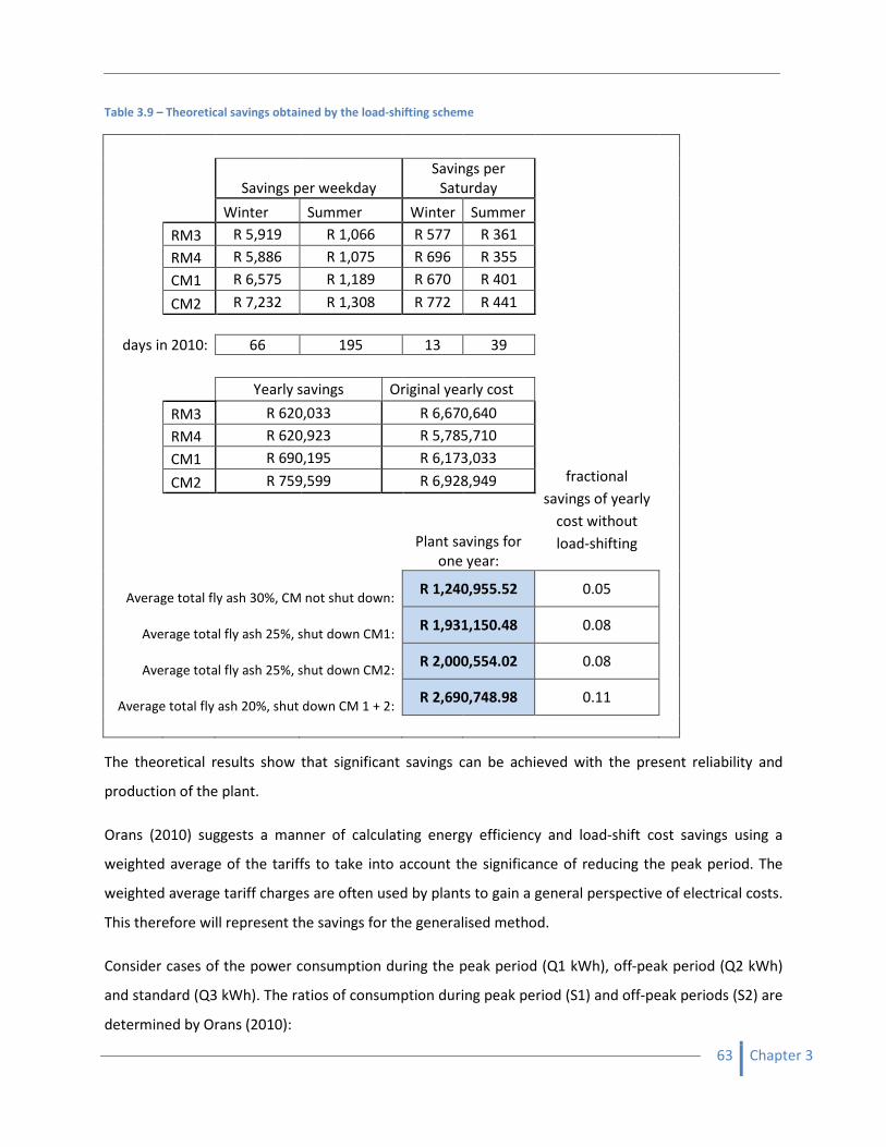
63 Chapter 3

Table 3.9 – Theoretical savings obtained by the load-shifting scheme

Savings per weekday

Savings per

Saturday

Winter Summer Winter Summer

RM3 R 5,919 R 1,066 R 577 R 361

RM4 R 5,886 R 1,075 R 696 R 355

CM1 R 6,575 R 1,189 R 670 R 401

CM2 R 7,232 R 1,308 R 772 R 441

days in 2010: 66 195 13 39

Yearly savings Original yearly cost

RM3 R 620,033 R 6,670,640

RM4 R 620,923 R 5,785,710

CM1 R 690,195 R 6,173,033

fractional

savings of yearly

cost without

load-shifting

CM2 R 759,599 R 6,928,949

Plant savings for

one year:

Average total fly ash 30%, CM not shut down: R 1,240,955.52 0.05

Average total fly ash 25%, shut down CM1: R 1,931,150.48 0.08

Average total fly ash 25%, shut down CM2: R 2,000,554.02 0.08

Average total fly ash 20%, shut down CM 1 + 2: R 2,690,748.98 0.11

The theoretical results show that significant savings can be achieved with the present reliability and

production of the plant.

Orans (2010) suggests a manner of calculating energy efficiency and load-shift cost savings using a

weighted average of the tariffs to take into account the significance of reducing the peak period. The

weighted average tariff charges are often used by plants to gain a general perspective of electrical costs.

This therefore will represent the savings for the generalised method.

Consider cases of the power consumption during the peak period (Q1 kWh), off-peak period (Q2 kWh)

and standard (Q3 kWh). The ratios of consumption during peak period (S1) and off-peak periods (S2) are

determined by Orans (2010):

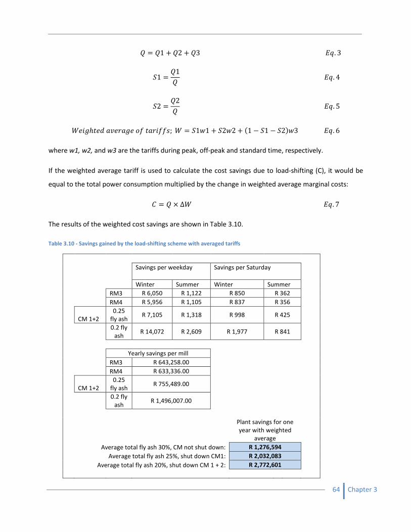
64 Chapter 3

� �1 � �2 � �3 )*. 3

�1 �1

� )*. 4

�2 �2

� )*. 5

�� ; � �1 1 � �2 2 � !1 " �1 " �2# 3 )*. 6

where w1, w2, and w3 are the tariffs during peak, off-peak and standard time, respectively.

If the weighted average tariff is used to calculate the cost savings due to load-shifting (C), it would be

equal to the total power consumption multiplied by the change in weighted average marginal costs:

� � $ ∆� )*. 7

The results of the weighted cost savings are shown in Table 3.10.

Table 3.10 - Savings gained by the load-shifting scheme with averaged tariffs

Savings per weekday

Savings per Saturday

Winter Summer Winter Summer

RM3 R 6,050 R 1,122 R 850 R 362

RM4 R 5,956 R 1,105 R 837 R 356

CM 1+2

0.25

fly ash R 7,105 R 1,318 R 998 R 425

0.2 fly

ash R 14,072 R 2,609 R 1,977 R 841

Yearly savings per mill

RM3 R 643,258.00

RM4 R 633,336.00

CM 1+2

0.25

fly ash R 755,489.00

0.2 fly

ash R 1,496,007.00

Plant savings for one

year with weighted

average

Average total fly ash 30%, CM not shut down: R 1,276,594

Average total fly ash 25%, shut down CM1: R 2,032,083

Average total fly ash 20%, shut down CM 1 + 2: R 2,772,601

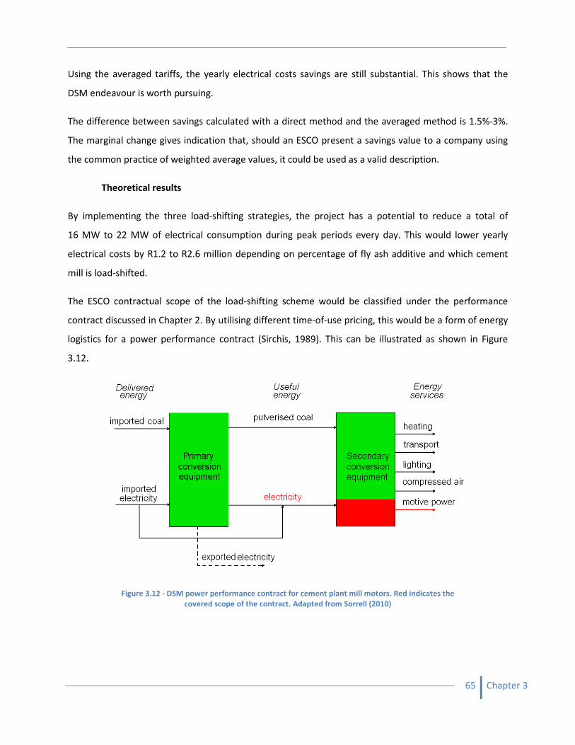
65 Chapter 3

Using the averaged tariffs, the yearly electrical costs savings are still substantial. This shows that the

DSM endeavour is worth pursuing.

The difference between savings calculated with a direct method and the averaged method is 1.5%-3%.

The marginal change gives indication that, should an ESCO present a savings value to a company using

the common practice of weighted average values, it could be used as a valid description.

Theoretical results

By implementing the three load-shifting strategies, the project has a potential to reduce a total of

16 MW to 22 MW of electrical consumption during peak periods every day. This would lower yearly

electrical costs by R1.2 to R2.6 million depending on percentage of fly ash additive and which cement

mill is load-shifted.

The ESCO contractual scope of the load-shifting scheme would be classified under the performance

contract discussed in Chapter 2. By utilising different time-of-use pricing, this would be a form of energy

logistics for a power performance contract (Sirchis, 1989). This can be illustrated as shown in Figure

3.12.

Figure 3.12 - DSM power performance contract for cement plant mill motors. Red indicates the

covered scope of the contract. Adapted from Sorrell (2010)

66 Chapter 3

The load-shifting scheme of the mill motors does not improve the motive power energy efficiency of the

plant. It does however improve the logistics of the useful energy that is used in the motive power,

hence, resulting in the ESCO contract block diagram shown in Figure 3.12.

3.6. Pilot study

A pilot study can be performed on the plant to verify whether the load-shifting scheme can achieve the

predicted cost savings. The cement plant under investigation currently has an integrated operating and

monitoring system. The load-shifting strategy can be implemented by using this system.

If all the influential factors discussed show that load-shifting is possible, the mills can be turned off

during peak periods and used more regularly during off-peak periods for a number of hours. The SCADA

system used to supply the plant data will again be used to record how the load-shifting affects the

production and power consumption. Using this data, the verification of the simulation model can be

achieved.

3.7. Conclusion

The investigation shows that there is great potential for reducing peak time usage for both the raw mills

and cement mills in the plant. The strategy is dynamic in that it can be chosen to be implemented if

conditions are appropriate. It can also be increased to the morning peak periods should there be a lower

level of incident hours.

The daily calculation of the baseline and adjustment to the load-shifting strategy will allow production to

continue while adhering to the DSM regulations. This will result in a flexible load-shifting project which

has the potential for substantial electrical cost savings.

3.8. References

Eskom, 2010. Tariffs & Charges 2010/11. Eskom, PO Box 1091, Johannesburg, 2000, South Africa.

Human, M., 2010. Personnel communication with electrical manager at Lafarge Lichtenburg. Manana

Road, Industrial Sites, Lichtenburg 2740, South Africa.

Meltese, C., Pistolesi, C., Bravo, A., Cella, F., Cerulli, T., Salvioni, D., 2007. A case history: Effect of

moisture on the setting behaviour of a Portland cement reacting with an alkali-free accelerator.

Cement and Concrete Research 37 (6), 856-865.

67 Chapter 3


report. Canadian Indusrty Programme for Energy Conservation. c/o Natural Resources Canada,

580 Booth Street, 12th




Paulus, M., Borggrefe, F., 2011. The potential of demand-side management in energy-intensive

industries for electricity markets in Germany. Applied Energy 88 (2), 432-44.

Potgieter-Vermaak, S.S., Potgieter, J.H., Worobiec, A., van Grieken, R., Marjanovic, L., Moeketsi, S., 2007.

Fingerprinting of South African ordinary Portland cements, cement blends and mortars for

identification purposes – Discrimination with starplots and PCA. Cement and Concrete Research

37, 834-843.

Sirchis, J., 1989. Energy efficiency in the cement industry. Proceedings of a seminar organized by the

Commission of the European Communities, Directorate-General from Energy and CIMPOR

Cimentos de Portugal E.P. with the co-operation of Cembureau European Cement Association,

Oporto, Portugal.


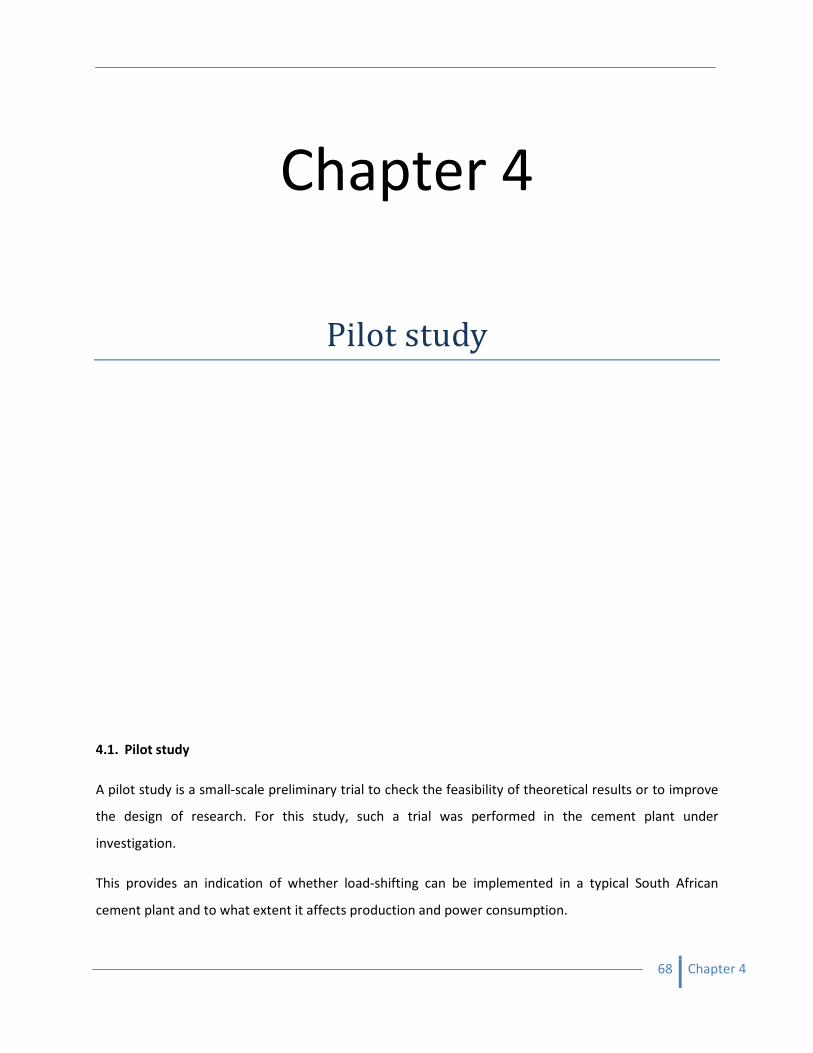
68 Chapter 4

Chapter 4

Pilot study

4.1. Pilot study

A pilot study is a small-scale preliminary trial to check the feasibility of theoretical results or to improve

the design of research. For this study, such a trial was performed in the cement plant under

investigation.

This provides an indication of whether load-shifting can be implemented in a typical South African

cement plant and to what extent it affects production and power consumption.

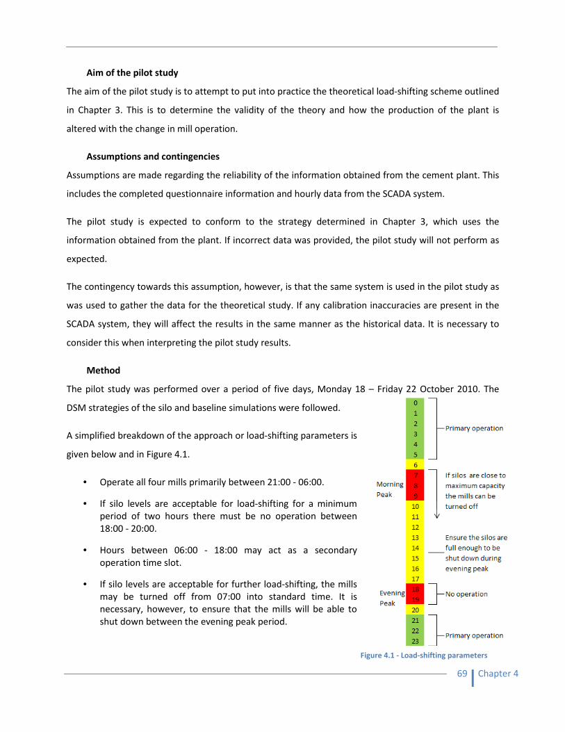
69 Chapter 4

Aim of the pilot study

The aim of the pilot study is to attempt to put into practice the theoretical load-shifting scheme outlined

in Chapter 3. This is to determine the validity of the theory and how the production of the plant is

altered with the change in mill operation.

Assumptions and contingencies

Assumptions are made regarding the reliability of the information obtained from the cement plant. This

includes the completed questionnaire information and hourly data from the SCADA system.

The pilot study is expected to conform to the strategy determined in Chapter 3, which uses the

information obtained from the plant. If incorrect data was provided, the pilot study will not perform as

expected.

The contingency towards this assumption, however, is that the same system is used in the pilot study as

was used to gather the data for the theoretical study. If any calibration inaccuracies are present in the

SCADA system, they will affect the results in the same manner as the historical data. It is necessary to

consider this when interpreting the pilot study results.

Method

The pilot study was performed over a period of five days, Monday 18 – Friday 22 October 2010. The

DSM strategies of the silo and baseline simulations were followed.

A simplified breakdown of the approach or load-shifting parameters is

given below and in Figure 4.1.

• Operate all four mills primarily between 21:00 - 06:00.

• If silo levels are acceptable for load-shifting for a minimum

period of two hours there must be no operation between

18:00 - 20:00.

• Hours between 06:00 - 18:00 may act as a secondary

operation time slot.

• If silo levels are acceptable for further load-shifting, the mills

may be turned off from 07:00 into standard time. It is

necessary, however, to ensure that the mills will be able to

shut down between the evening peak period.

Figure 4.1 - Load-shifting parameters

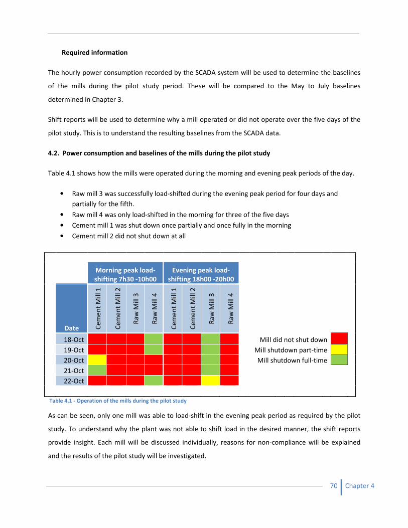
70 Chapter 4

Required information

The hourly power consumption recorded by the SCADA system will be used to determine the baselines

of the mills during the pilot study period. These will be compared to the May to July baselines

determined in Chapter 3.

Shift reports will be used to determine why a mill operated or did not operate over the five days of the

pilot study. This is to understand the resulting baselines from the SCADA data.

4.2. Power consumption and baselines of the mills during the pilot study

Table 4.1 shows how the mills were operated during the morning and evening peak periods of the day.

• Raw mill 3 was successfully load-shifted during the evening peak period for four days and

partially for the fifth.

• Raw mill 4 was only load-shifted in the morning for three of the five days

• Cement mill 1 was shut down once partially and once fully in the morning

• Cement mill 2 did not shut down at all

Table 4.1 - Operation of the mills during the pilot study

As can be seen, only one mill was able to load-shift in the evening peak period as required by the pilot

study. To understand why the plant was not able to shift load in the desired manner, the shift reports

provide insight. Each mill will be discussed individually, reasons for non-compliance will be explained

and the results of the pilot study will be investigated.

Morning peak load-

shifting 7h30 -10h00

Evening peak load-

shifting 18h00 -20h00

Date Ce

me

nt

Mil

l 1

Ce

me

nt

Mil

l 2

Ra

w M

ill

3

Ra

w M

ill

4

Ce

me

nt

Mil

l 1

Ce

me

nt

Mil

l 2

Ra

w M

ill

3

Ra

w M

ill

4

18-Oct

Mill did not shut down

19-Oct

Mill shutdown part-time

20-Oct

Mill shutdown full-time

21-Oct

22-Oct

71 Chapter 4

Cement mill 1

SCADA data were used to develop Figure 4.2. The figure presents the power consumption, and therefore

the operation, of cement mill 1 during the pilot study. The light red shaded area represents the evening

peak periods when the mill should have been shut down and electrical consumption equal to zero. The

graph also provides indication as to when and why incident hours occurred.

Figure 4.2 - CM1 power consumption pilot study

As can be seen in the graph, cement mill 1 did not once shut down during the evening peak period. At

the time of the pilot study, the plant production manager increased production of the cement mills. As a

result they were not allowed to be shut down for load-shifting so as to meet the raised production

demand.

However, cement mill 1 had a total of 23.75 incident hours during the week and as a result produced the

baseline shown in Figure 4.3. Fewer incident hours were experienced during the evening peak period

and as a result were used to make up for the unscheduled, lost production time. Coincidentally, this

caused a very high electrical usage during the peak period which is completely opposite to what was

sought in the pilot study. Because of this, it is most likely that the cost to operate the mill is higher than

that experienced during the investigation. This will be addressed later in the chapter.

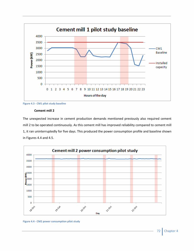
72 Chapter 4

Figure 4.3 - CM1 pilot study baseline

Cement mill 2

The unexpected increase in cement production demands mentioned previously also required cement

mill 2 to be operated continuously. As this cement mill has improved reliability compared to cement mill

1, it ran uninterruptedly for five days. This produced the power consumption profile and baseline shown

in Figures 4.4 and 4.5.

Figure 4.4 - CM2 power consumption pilot study

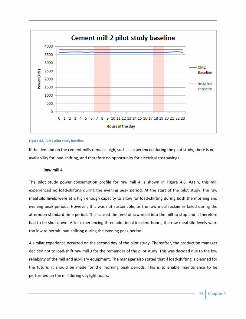
73 Chapter 4

Figure 4.5 - CM2 pilot study baseline

If the demand on the cement mills remains high, such as experienced during the pilot study, there is no

availability for load-shifting, and therefore no opportunity for electrical cost savings.

Raw mill 4

The pilot study power consumption profile for raw mill 4 is shown in Figure 4.6. Again, this mill

experienced no load-shifting during the evening peak period. At the start of the pilot study, the raw

meal silo levels were at a high enough capacity to allow for load-shifting during both the morning and

evening peak periods. However, this was not sustainable, as the raw meal reclaimer failed during the

afternoon standard time period. This caused the feed of raw meal into the mill to stop and it therefore

had to be shut down. After experiencing three additional incident hours, the raw meal silo levels were

too low to permit load-shifting during the evening peak period.

A similar experience occurred on the second day of the pilot study. Thereafter, the production manager

decided not to load-shift raw mill 3 for the remainder of the pilot study. This was decided due to the low

reliability of the mill and auxiliary equipment. The manager also stated that if load-shifting is planned for

the future, it should be made for the morning peak periods. This is to enable maintenance to be

performed on the mill during daylight hours.

74 Chapter 4

Figure 4.6 - RM4 power consumption pilot study

The baseline of raw mill 4 produced during the pilot study can be seen in Figure 4.7. It shows that

although there was a 58% reduction in consumption for a portion of the morning peak period, there was

none in the evening. This again does not meet the objectives of the load-shifting scheme. With the high

level of unreliability of the mill, it is difficult to achieve planned load-shifting and cost savings.

Figure 4.7 - RM4 pilot study baseline

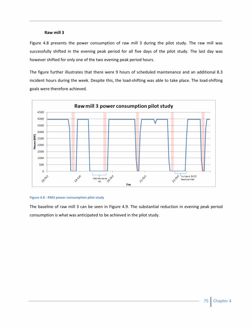
75 Chapter 4

Raw mill 3

Figure 4.8 presents the power consumption of raw mill 3 during the pilot study. The raw mill was

successfully shifted in the evening peak period for all five days of the pilot study. The last day was

however shifted for only one of the two evening peak period hours.

The figure further illustrates that there were 9 hours of scheduled maintenance and an additional 8.3

incident hours during the week. Despite this, the load-shifting was able to take place. The load-shifting

goals were therefore achieved.

Figure 4.8 - RM3 power consumption pilot study

The baseline of raw mill 3 can be seen in Figure 4.9. The substantial reduction in evening peak period

consumption is what was anticipated to be achieved in the pilot study.

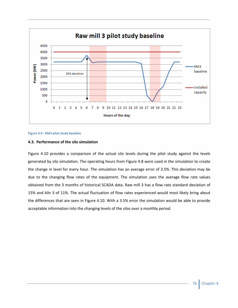
76 Chapter 4

Figure 4.9 - RM3 pilot study baseline

4.3. Performance of the silo simulation

Figure 4.10 provides a comparison of the actual silo levels during the pilot study against the levels

generated by silo simulation. The operating hours from Figure 4.8 were used in the simulation to create

the change in level for every hour. The simulation has an average error of 3.5%. This deviation may be

due to the changing flow rates of the equipment. The simulation uses the average flow rate values

obtained from the 3 months of historical SCADA data. Raw mill 3 has a flow rate standard deviation of

15% and kiln 3 of 11%. The actual fluctuation of flow rates experienced would most likely bring about

the differences that are seen in Figure 4.10. With a 3.5% error the simulation would be able to provide

acceptable information into the changing levels of the silos over a monthly period.

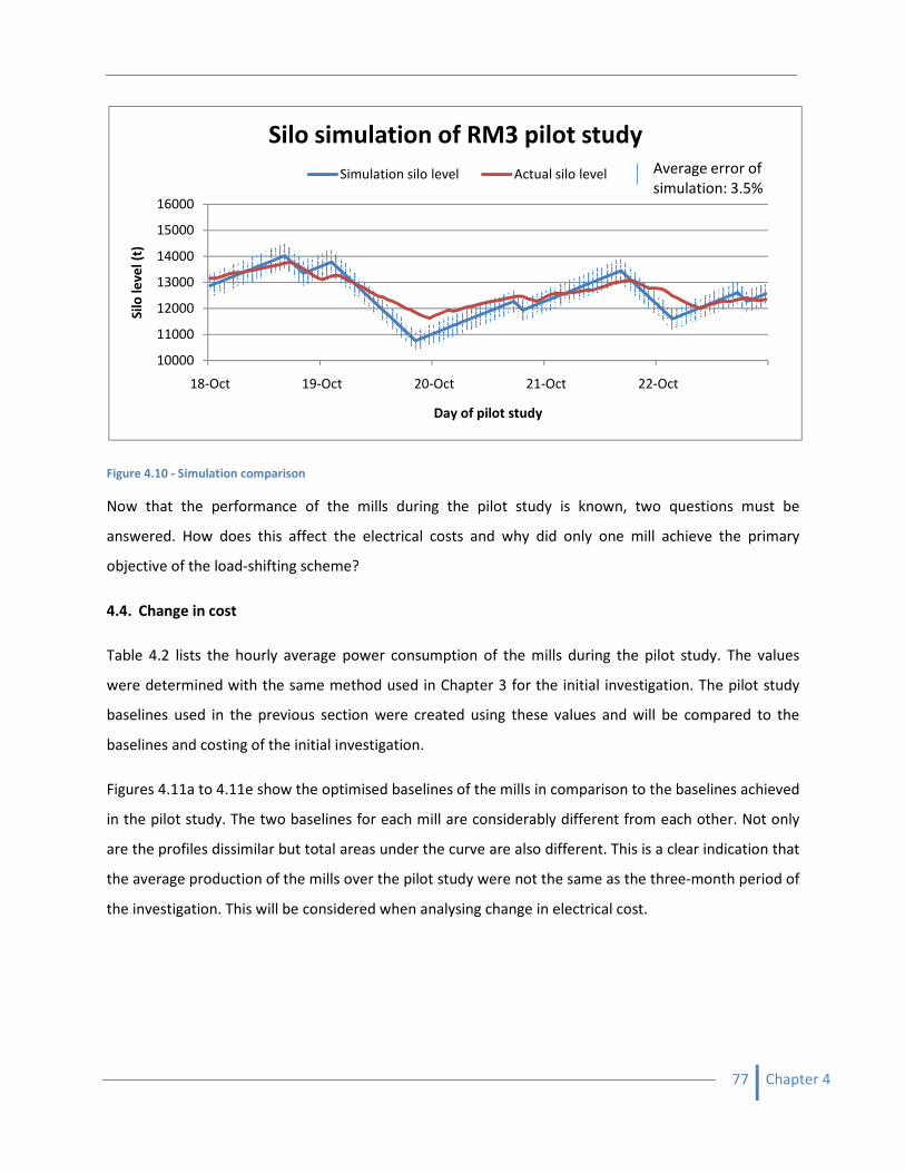
Figure 4.10 - Simulation comparison

Now that the performance of the mills during the pilot study is know

answered. How does this affect the electrical costs and why did only one mill achieve the

objective of the load-shifting scheme?

4.4. Change in cost

Table 4.2 lists the hourly average power consumption of the mills during the pilot study. The values

were determined with the same method

baselines used in the previous section were created using these values and will be compared to the

baselines and costing of the initial investigation.

Figures 4.11a to 4.11e show the optimised baselines of the mills in comparison to the baselines

in the pilot study. The two baselines for each mill are considerably different from each other. Not only

are the profiles dissimilar but total area

the average production of the mills over the pilot study were not the same as the three

the investigation. This will be considered

10000

11000

12000

13000

14000

15000

16000

18-Oct 19-Oct

Sil

o l

ev

el

(t)

Silo simulation of RM3 pilot study

Now that the performance of the mills during the pilot study is known, two questions must be

ow does this affect the electrical costs and why did only one mill achieve the

shifting scheme?

4.2 lists the hourly average power consumption of the mills during the pilot study. The values

etermined with the same method used in Chapter 3 for the initial investigation. The pi


baselines and costing of the initial investigation.

optimised baselines of the mills in comparison to the baselines


are the profiles dissimilar but total areas under the curve are also different. This is a clear indication that

mills over the pilot study were not the same as the three

considered when analysing change in electrical cost.

Oct 20-Oct 21-Oct 22-Oct

Day of pilot study

Silo simulation of RM3 pilot study

Simulation silo level Actual silo level Average error

simulation: 3.5%

77 Chapter 4

two questions must be

ow does this affect the electrical costs and why did only one mill achieve the primary

4.2 lists the hourly average power consumption of the mills during the pilot study. The values

used in Chapter 3 for the initial investigation. The pilot study


optimised baselines of the mills in comparison to the baselines achieved


also different. This is a clear indication that

mills over the pilot study were not the same as the three-month period of

Oct

Average error of

simulation: 3.5%

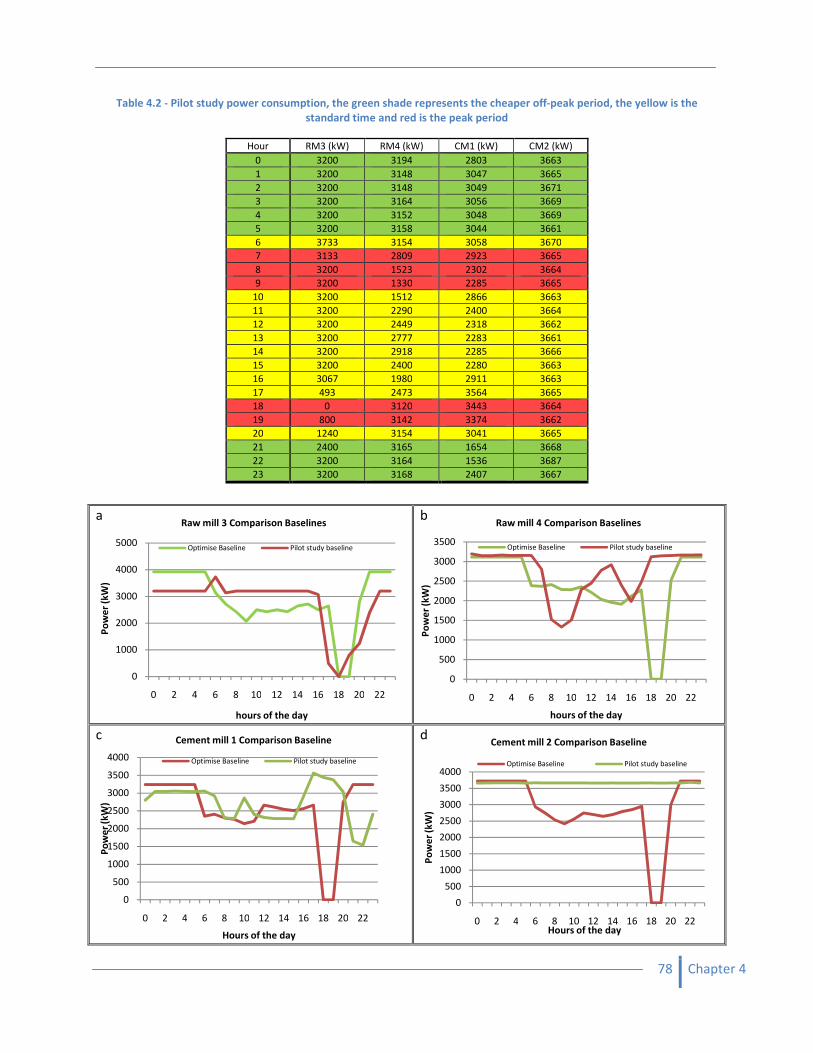
78 Chapter 4

0

500

1000

1500

2000

2500

3000

3500

4000

0 2 4 6 8 10 12 14 16 18 20 22

Po

we

r (k

W)

Hours of the day

Cement mill 1 Comparison Baseline

Optimise Baseline Pilot study baseline

0

500

1000

1500

2000

2500

3000

3500

4000

0 2 4 6 8 10 12 14 16 18 20 22

Po

we

r (k

W)

Hours of the day

Cement mill 2 Comparison Baseline


0

1000

2000

3000

4000

5000

0 2 4 6 8 10 12 14 16 18 20 22

Po

we

r (k

W)

hours of the day

Raw mill 3 Comparison Baselines


0

500

1000

1500

2000

2500

3000

3500

0 2 4 6 8 10 12 14 16 18 20 22

Po

we

r (k

W)

hours of the day

Raw mill 4 Comparison Baselines


Table 4.2 - Pilot study power consumption, the green shade represents the cheaper off-peak period, the yellow is the

standard time and red is the peak period

Hour RM3 (kW) RM4 (kW) CM1 (kW) CM2 (kW)

0 3200 3194 2803 3663

1 3200 3148 3047 3665

2 3200 3148 3049 3671

3 3200 3164 3056 3669

4 3200 3152 3048 3669

5 3200 3158 3044 3661

6 3733 3154 3058 3670

7 3133 2809 2923 3665

8 3200 1523 2302 3664

9 3200 1330 2285 3665

10 3200 1512 2866 3663

11 3200 2290 2400 3664

12 3200 2449 2318 3662

13 3200 2777 2283 3661

14 3200 2918 2285 3666

15 3200 2400 2280 3663

16 3067 1980 2911 3663

17 493 2473 3564 3665

18 0 3120 3443 3664

19 800 3142 3374 3662

20 1240 3154 3041 3665

21 2400 3165 1654 3668

22 3200 3164 1536 3687

23 3200 3168 2407 3667

a b

c d

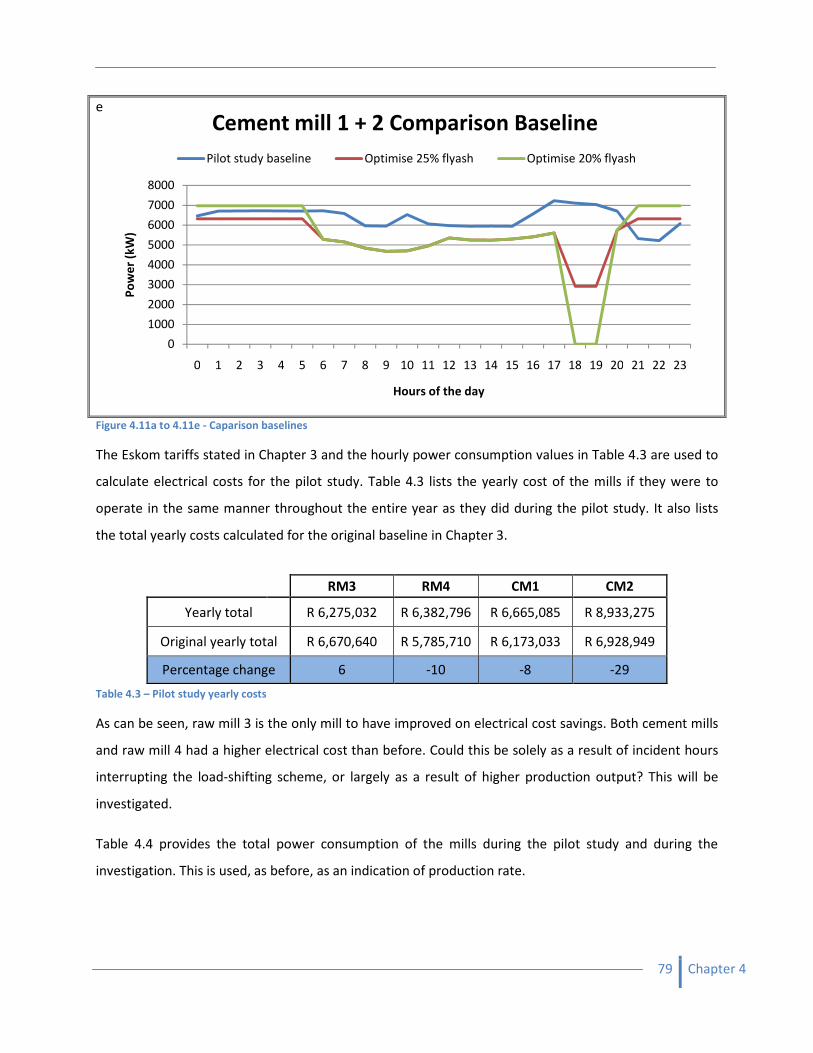
79 Chapter 4

0

1000

2000

3000

4000

5000

6000

7000

8000

0 1 2 3 4 5 6 7 8 9 10 11 12 13 14 15 16 17 18 19 20 21 22 23

Po

we

r (k

W)

Hours of the day

Cement mill 1 + 2 Comparison Baseline

Pilot study baseline Optimise 25% flyash Optimise 20% flyash

e

Figure 4.11a to 4.11e - Caparison baselines

The Eskom tariffs stated in Chapter 3 and the hourly power consumption values in Table 4.3 are used to

calculate electrical costs for the pilot study. Table 4.3 lists the yearly cost of the mills if they were to

operate in the same manner throughout the entire year as they did during the pilot study. It also lists

the total yearly costs calculated for the original baseline in Chapter 3.

Table 4.3 – Pilot study yearly costs

As can be seen, raw mill 3 is the only mill to have improved on electrical cost savings. Both cement mills

and raw mill 4 had a higher electrical cost than before. Could this be solely as a result of incident hours

interrupting the load-shifting scheme, or largely as a result of higher production output? This will be

investigated.

Table 4.4 provides the total power consumption of the mills during the pilot study and during the

investigation. This is used, as before, as an indication of production rate.

RM3 RM4 CM1 CM2

Yearly total R 6,275,032 R 6,382,796 R 6,665,085 R 8,933,275

Original yearly total R 6,670,640 R 5,785,710 R 6,173,033 R 6,928,949

Percentage change 6 -10 -8 -29

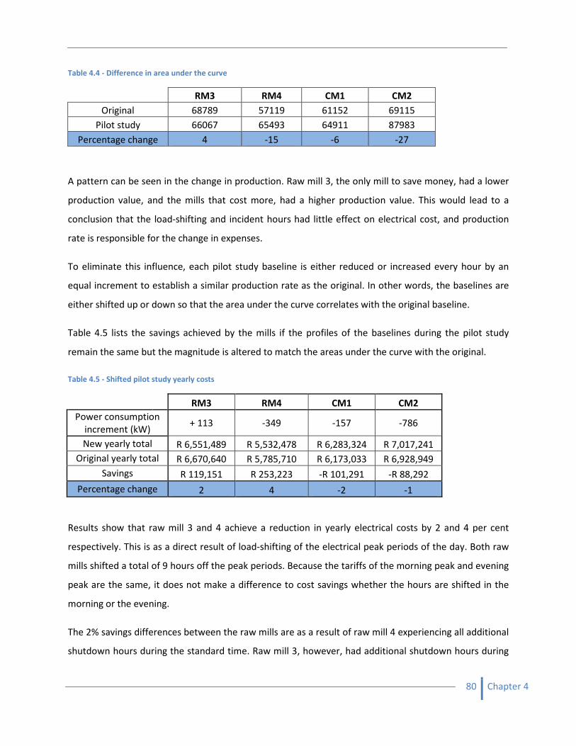
80 Chapter 4

Table 4.4 - Difference in area under the curve

RM3 RM4 CM1 CM2

Original 68789 57119 61152 69115

Pilot study 66067 65493 64911 87983

Percentage change 4 -15 -6 -27

A pattern can be seen in the change in production. Raw mill 3, the only mill to save money, had a lower

production value, and the mills that cost more, had a higher production value. This would lead to a

conclusion that the load-shifting and incident hours had little effect on electrical cost, and production

rate is responsible for the change in expenses.

To eliminate this influence, each pilot study baseline is either reduced or increased every hour by an

equal increment to establish a similar production rate as the original. In other words, the baselines are

either shifted up or down so that the area under the curve correlates with the original baseline.

Table 4.5 lists the savings achieved by the mills if the profiles of the baselines during the pilot study

remain the same but the magnitude is altered to match the areas under the curve with the original.

Table 4.5 - Shifted pilot study yearly costs

RM3 RM4 CM1 CM2

Power consumption

increment (kW) + 113 -349 -157 -786

New yearly total R 6,551,489 R 5,532,478 R 6,283,324 R 7,017,241

Original yearly total R 6,670,640 R 5,785,710 R 6,173,033 R 6,928,949

Savings R 119,151 R 253,223 -R 101,291 -R 88,292

Percentage change 2 4 -2 -1

Results show that raw mill 3 and 4 achieve a reduction in yearly electrical costs by 2 and 4 per cent

respectively. This is as a direct result of load-shifting of the electrical peak periods of the day. Both raw

mills shifted a total of 9 hours off the peak periods. Because the tariffs of the morning peak and evening

peak are the same, it does not make a difference to cost savings whether the hours are shifted in the

morning or the evening.

The 2% savings differences between the raw mills are as a result of raw mill 4 experiencing all additional

shutdown hours during the standard time. Raw mill 3, however, had additional shutdown hours during

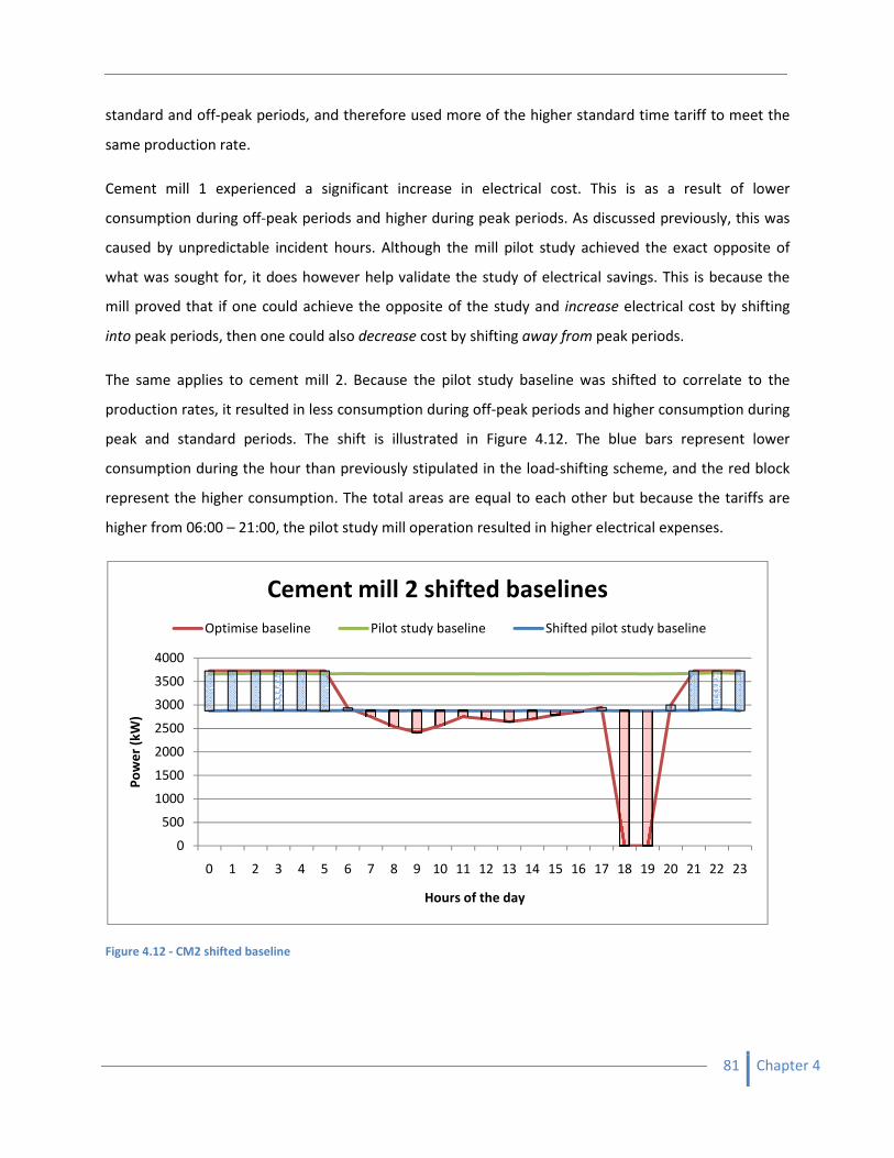
standard and off-peak periods, and therefore used

same production rate.

Cement mill 1 experienced a significant increase in electrical cost

consumption during off-peak perio

caused by unpredictable incident hours. Although the mill pilot study achieved the exact opposite of

what was sought for, it does however help validate the study of electrical savings. This is because the

mill proved that if one could achieve the opposite of the study and

into peak periods, then one could also

The same applies to cement mill 2. Because the pilot study baseline was shifted to correlate to

production rates, it resulted in less consumption during off

peak and standard periods. The shift is illustrated in Figure 4.1

consumption during the hour than previously stipu

represent the higher consumption. The total areas are equal to each other but because the tariffs are

higher from 06:00 – 21:00, the pilot study mill operation resulted in higher electrical expenses.

Figure 4.12 - CM2 shifted baseline

0

500

1000

1500

2000

2500

3000

3500

4000

0 1 2 3 4 5

Po

we

r (k

W)

Cement mill 2 shifted baselines

Optimise baseline

peak periods, and therefore used more of the higher standard time tariff to meet the

Cement mill 1 experienced a significant increase in electrical cost. This is as a result of

peak periods and higher during peak periods. As discussed pre

incident hours. Although the mill pilot study achieved the exact opposite of


ieve the opposite of the study and increase electrical cost by shifting

peak periods, then one could also decrease cost by shifting away from peak periods.

The same applies to cement mill 2. Because the pilot study baseline was shifted to correlate to

production rates, it resulted in less consumption during off-peak periods and higher consumption during

peak and standard periods. The shift is illustrated in Figure 4.12. The blue bars represent l

consumption during the hour than previously stipulated in the load-shifting scheme, and the red block


the pilot study mill operation resulted in higher electrical expenses.

6 7 8 9 10 11 12 13 14 15 16 17 18 19 20

Hours of the day

Cement mill 2 shifted baselines

Pilot study baseline Shifted pilot study baseline

81 Chapter 4

more of the higher standard time tariff to meet the

as a result of lower

s discussed previously, this was

incident hours. Although the mill pilot study achieved the exact opposite of


electrical cost by shifting

peak periods.

The same applies to cement mill 2. Because the pilot study baseline was shifted to correlate to the

peak periods and higher consumption during

. The blue bars represent lower

ing scheme, and the red block


the pilot study mill operation resulted in higher electrical expenses.

20 21 22 23

Shifted pilot study baseline

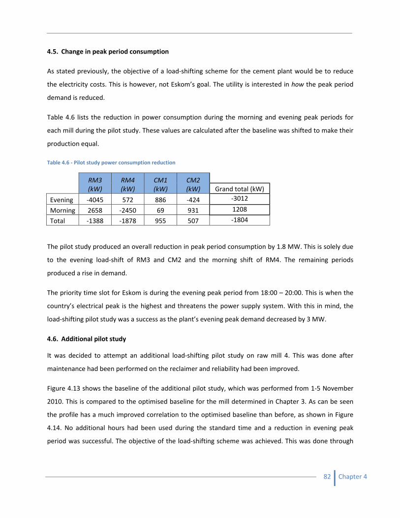
82 Chapter 4

4.5. Change in peak period consumption

As stated previously, the objective of a load-shifting scheme for the cement plant would be to reduce

the electricity costs. This is however, not Eskom’s goal. The utility is interested in how the peak period

demand is reduced.

Table 4.6 lists the reduction in power consumption during the morning and evening peak periods for

each mill during the pilot study. These values are calculated after the baseline was shifted to make their

production equal.

Table 4.6 - Pilot study power consumption reduction

RM3

(kW)

RM4

(kW)

CM1

(kW)

CM2

(kW)

Grand total (kW)

Evening -4045 572 886 -424 -3012

Morning 2658 -2450 69 931 1208

Total -1388 -1878 955 507 -1804

The pilot study produced an overall reduction in peak period consumption by 1.8 MW. This is solely due

to the evening load-shift of RM3 and CM2 and the morning shift of RM4. The remaining periods

produced a rise in demand.

The priority time slot for Eskom is during the evening peak period from 18:00 – 20:00. This is when the

country’s electrical peak is the highest and threatens the power supply system. With this in mind, the

load-shifting pilot study was a success as the plant’s evening peak demand decreased by 3 MW.

4.6. Additional pilot study

It was decided to attempt an additional load-shifting pilot study on raw mill 4. This was done after

maintenance had been performed on the reclaimer and reliability had been improved.

Figure 4.13 shows the baseline of the additional pilot study, which was performed from 1-5 November

2010. This is compared to the optimised baseline for the mill determined in Chapter 3. As can be seen

the profile has a much improved correlation to the optimised baseline than before, as shown in Figure

4.14. No additional hours had been used during the standard time and a reduction in evening peak

period was successful. The objective of the load-shifting scheme was achieved. This was done through

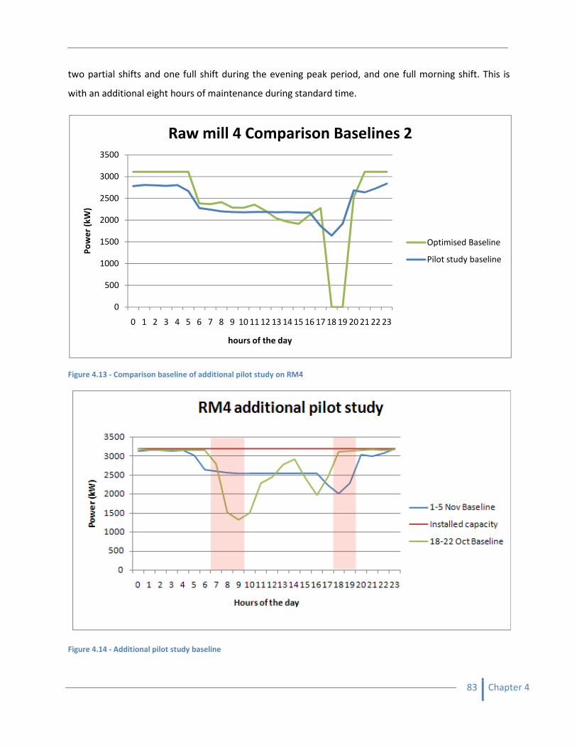
83 Chapter 4

two partial shifts and one full shift during the evening peak period, and one full morning shift. This is

with an additional eight hours of maintenance during standard time.

Figure 4.13 - Comparison baseline of additional pilot study on RM4

Figure 4.14 - Additional pilot study baseline

0

500

1000

1500

2000

2500

3000

3500

0 1 2 3 4 5 6 7 8 9 10 11 12 13 14 15 16 17 18 19 20 21 22 23

Po

we

r (k

W)

hours of the day

Raw mill 4 Comparison Baselines 2

Optimised Baseline

Pilot study baseline

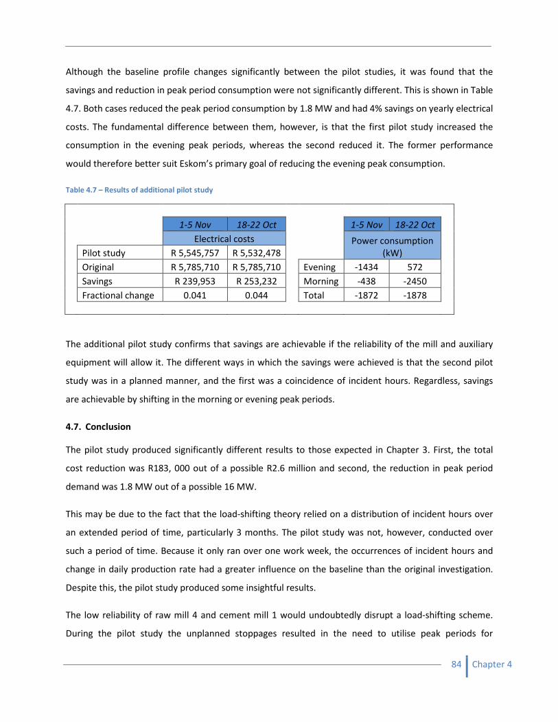
84 Chapter 4

Although the baseline profile changes significantly between the pilot studies, it was found that the

savings and reduction in peak period consumption were not significantly different. This is shown in Table

4.7. Both cases reduced the peak period consumption by 1.8 MW and had 4% savings on yearly electrical

costs. The fundamental difference between them, however, is that the first pilot study increased the

consumption in the evening peak periods, whereas the second reduced it. The former performance

would therefore better suit Eskom’s primary goal of reducing the evening peak consumption.

Table 4.7 – Results of additional pilot study

1-5 Nov 18-22 Oct

1-5 Nov 18-22 Oct

Electrical costs

Power consumption

(kW)

Pilot study R 5,545,757 R 5,532,478

Original R 5,785,710 R 5,785,710

Evening -1434 572

Savings R 239,953 R 253,232

Morning -438 -2450

Fractional change 0.041 0.044

Total -1872 -1878

The additional pilot study confirms that savings are achievable if the reliability of the mill and auxiliary

equipment will allow it. The different ways in which the savings were achieved is that the second pilot

study was in a planned manner, and the first was a coincidence of incident hours. Regardless, savings

are achievable by shifting in the morning or evening peak periods.

4.7. Conclusion

The pilot study produced significantly different results to those expected in Chapter 3. First, the total

cost reduction was R183, 000 out of a possible R2.6 million and second, the reduction in peak period

demand was 1.8 MW out of a possible 16 MW.

This may be due to the fact that the load-shifting theory relied on a distribution of incident hours over

an extended period of time, particularly 3 months. The pilot study was not, however, conducted over

such a period of time. Because it only ran over one work week, the occurrences of incident hours and

change in daily production rate had a greater influence on the baseline than the original investigation.

Despite this, the pilot study produced some insightful results.

The low reliability of raw mill 4 and cement mill 1 would undoubtedly disrupt a load-shifting scheme.

During the pilot study the unplanned stoppages resulted in the need to utilise peak periods for

85 Chapter 4

production. In the case of the cement mills, it resulted in an increase in electrical costs compared to

those calculated with the original baseline. This does not however provide grounds to dismiss savings

opportunities. They are unfortunately highly dependent on a daily adaption based on incident hours and

silo levels. The mills, although unreliable, are still capable of load-shifting and energy savings. This was

shown in the additional pilot study performed on raw mill 4.

Further to this, the increase in production demand on the cement mills resulted in a planned

cancellation of the load-shifting scheme. If a change in cement production demand requires an increase

in production, and material silos can support it, then the cement mills will not be shut down. During this

time, there is no opportunity for energy cost savings. Should demand be reduced the cement mills may

be able to shift load. This was not the case, however, during the pilot study.

Raw mill 3 produced promising results. The evening peak period shutdowns reduced the anticipated

yearly electrical costs by 2% and reduced demand by 1.88 MW. The mill was still able to achieve the

load-shifting scheme with an additional 8.3 hours of incidents and scheduled maintenance.

The pilot study, therefore, provided three cases:

• Successful load-shifting

• Unsuccessful load-shifting due to incident hours

• Unsuccessful load-shifting due to raised production demand

In conclusion, the pilot study was successful in providing insight into how load-shifting may affect, or be

affected, by plant operation and equipment reliability.

86 Chapter 5

Chapter 5

Conclusion

5.1. Revision of the research goal

South Africa is under threat of electricity shortages in the near future, and Eskom hopes to reduce the

demand to avoid future implications, such as rolling blackouts. After performing a literature survey on

global energy efficiency, it became evident that there are several opportunities for electrical energy

savings within the cement industry. To what extent can the South African industry exploit these benefits

and help Eskom reduce the demand? This is what was set out to be investigated in this study.

The research scope covered an investigation into electricity efficiency options that are applicable to the

typical South African cement plant. It also evaluated the opportunity of load-shifting for a particular

cement plant. Following these investigations, it is now possible to establish what opportunities there are

for South Africa, and to provide recommendations for the future. This is what is discussed in this final

chapter of the dissertation.

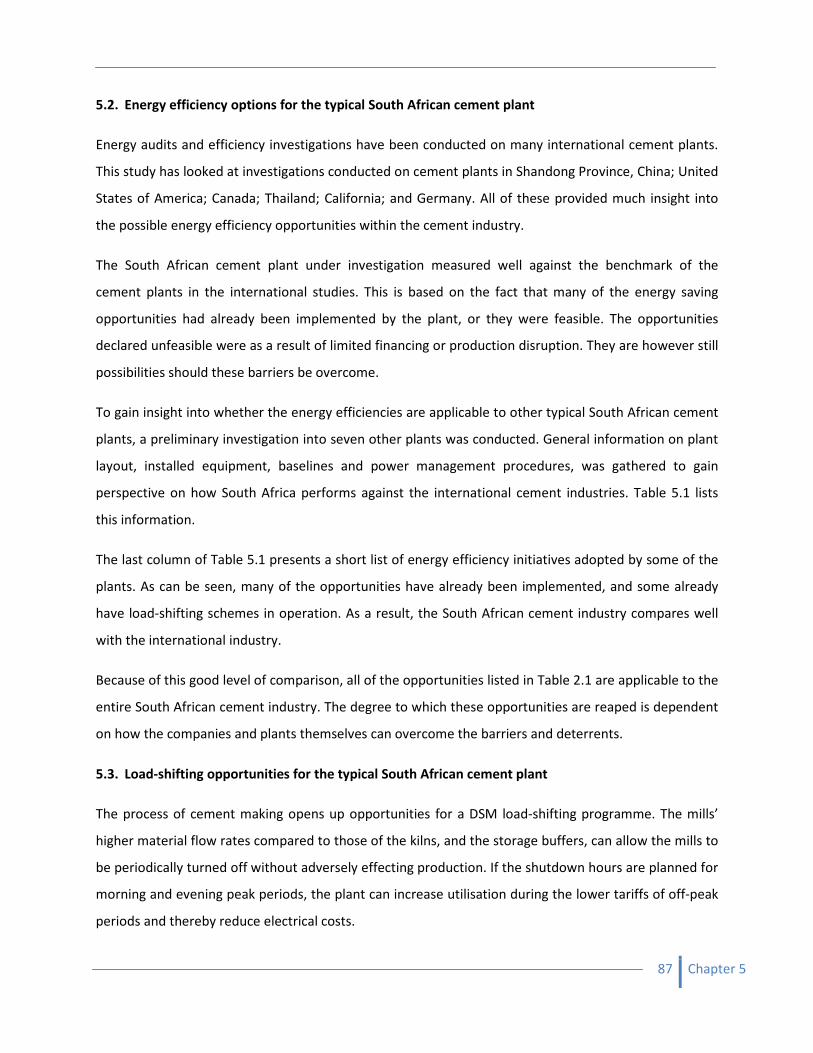
87 Chapter 5

5.2. Energy efficiency options for the typical South African cement plant

Energy audits and efficiency investigations have been conducted on many international cement plants.

This study has looked at investigations conducted on cement plants in Shandong Province, China; United

States of America; Canada; Thailand; California; and Germany. All of these provided much insight into

the possible energy efficiency opportunities within the cement industry.

The South African cement plant under investigation measured well against the benchmark of the

cement plants in the international studies. This is based on the fact that many of the energy saving

opportunities had already been implemented by the plant, or they were feasible. The opportunities

declared unfeasible were as a result of limited financing or production disruption. They are however still

possibilities should these barriers be overcome.

To gain insight into whether the energy efficiencies are applicable to other typical South African cement

plants, a preliminary investigation into seven other plants was conducted. General information on plant

layout, installed equipment, baselines and power management procedures, was gathered to gain

perspective on how South Africa performs against the international cement industries. Table 5.1 lists

this information.

The last column of Table 5.1 presents a short list of energy efficiency initiatives adopted by some of the

plants. As can be seen, many of the opportunities have already been implemented, and some already

have load-shifting schemes in operation. As a result, the South African cement industry compares well

with the international industry.

Because of this good level of comparison, all of the opportunities listed in Table 2.1 are applicable to the

entire South African cement industry. The degree to which these opportunities are reaped is dependent

on how the companies and plants themselves can overcome the barriers and deterrents.

5.3. Load-shifting opportunities for the typical South African cement plant

The process of cement making opens up opportunities for a DSM load-shifting programme. The mills’

higher material flow rates compared to those of the kilns, and the storage buffers, can allow the mills to

be periodically turned off without adversely effecting production. If the shutdown hours are planned for

morning and evening peak periods, the plant can increase utilisation during the lower tariffs of off-peak

periods and thereby reduce electrical costs.

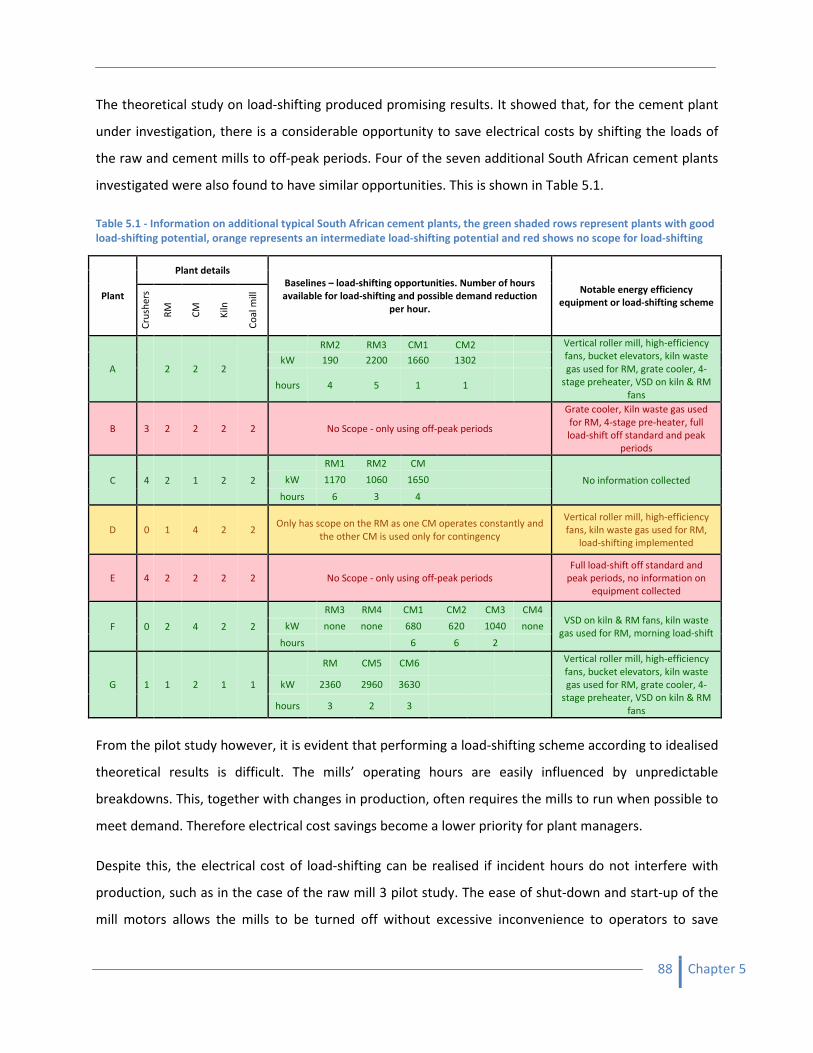
88 Chapter 5

The theoretical study on load-shifting produced promising results. It showed that, for the cement plant

under investigation, there is a considerable opportunity to save electrical costs by shifting the loads of

the raw and cement mills to off-peak periods. Four of the seven additional South African cement plants

investigated were also found to have similar opportunities. This is shown in Table 5.1.

Table 5.1 - Information on additional typical South African cement plants, the green shaded rows represent plants with good

load-shifting potential, orange represents an intermediate load-shifting potential and red shows no scope for load-shifting

From the pilot study however, it is evident that performing a load-shifting scheme according to idealised

theoretical results is difficult. The mills’ operating hours are easily influenced by unpredictable

breakdowns. This, together with changes in production, often requires the mills to run when possible to

meet demand. Therefore electrical cost savings become a lower priority for plant managers.

Despite this, the electrical cost of load-shifting can be realised if incident hours do not interfere with

production, such as in the case of the raw mill 3 pilot study. The ease of shut-down and start-up of the

mill motors allows the mills to be turned off without excessive inconvenience to operators to save

Plant

Plant details

Baselines – load-shifting opportunities. Number of hours

available for load-shifting and possible demand reduction

per hour.

Notable energy efficiency

equipment or load-shifting scheme

Cru

she

rs

RM

CM

Kiln

Co

al m

ill

A 2 2 2

RM2 RM3 CM1 CM2 Vertical roller mill, high-efficiency

fans, bucket elevators, kiln waste

gas used for RM, grate cooler, 4-

stage preheater, VSD on kiln & RM

fans

kW 190 2200 1660 1302

hours 4 5 1 1

B 3 2 2 2 2 No Scope - only using off-peak periods

Grate cooler, Kiln waste gas used

for RM, 4-stage pre-heater, full

load-shift off standard and peak

periods

C 4 2 1 2 2

RM1 RM2 CM

No information collected kW 1170 1060 1650

hours 6 3 4

D 0 1 4 2 2 Only has scope on the RM as one CM operates constantly and

the other CM is used only for contingency

Vertical roller mill, high-efficiency

fans, kiln waste gas used for RM,

load-shifting implemented

E 4 2 2 2 2 No Scope - only using off-peak periods

Full load-shift off standard and

peak periods, no information on

equipment collected

F 0 2 4 2 2

RM3 RM4 CM1 CM2 CM3 CM4 VSD on kiln & RM fans, kiln waste

gas used for RM, morning load-shift kW none none 680 620 1040 none

hours 6 6 2

G 1 1 2 1 1

RM CM5 CM6 Vertical roller mill, high-efficiency

fans, bucket elevators, kiln waste

gas used for RM, grate cooler, 4-

stage preheater, VSD on kiln & RM

fans

kW 2360 2960 3630

hours 3 2 3

89 Chapter 5

money. For cement mills, however, the influence of mill temperature over the cement setting quality

may deter cement plants from initiating a load-shifting scheme.

5.4. Recommendations

It is therefore suggested that a flexible load-shifting scheme be developed with more focus on load-

shifting hours than used in Chapter 3. The previous silo simulation took into account the changing

incident hours of the mills and auxiliary equipment, but it did not allow for an adjustable load-shifting

scheme.

For example, previous results suggested that although 4 hours of load-shifting were possible, the

baselines would only allow 2 hours of evening peak period shutdown every day, with a few hours

available during the month to allow for extra incidents or other load-shifting during morning peak

periods. A new simulation was created to adjust for the part of the day during which the load-shifting

hours occur, morning or evening, and how many times during the month.

In this way, the simulation can be used in a supplementary, dynamic manner and not only calculate a

number of hours for every weekday. This would also improve relevance to the morning load-shifts

required by the less reliable mills, such as preferred for raw mill 4 in the investigated plant.

Figure 5.1 is a snap shot of the simulation operating window. A full description can be found in Appendix

E. As can be seen in the expansion box, it provides a choice as to when the load-shifting shutdowns

occur. In this example, the mill can, not only, be shut down every weekday for 2 hours during the

evening peak period, but also 3 hours in the morning for three days a week.

This would provide improved flexibility to incident hours that prevent planned load-shifting from

occurring. The simulation still relies on an averaging of incident hours over the 31 days, but the

improved resolution does, however, serves as an aid to improve the flexibility of the load-shifting

scheme.

90 Chapter 5

Figure 5.1 - Improved silo simulation

5.5. Final Conclusion

There are substantial opportunities for energy efficiency and cost savings within the cement industry.

Many of the energy efficiency options, however, require large financial expenditures and are highly

disruptive to production during installation. If the barriers against such opportunities are overcome, the

companies can reap the benefits of significant electrical demand reductions.

Load-shifting provides a good opportunity in the cement making process to save electrical cost. This is

however highly dependent on the reliability of the mills, levels of material and the current market

demand. Load-shifting schemes should therefore be highly adaptable on a daily basis to shift load when

possible.

91 Chapter 5

Because most raw and cement mill motors have power outputs in the order of megawatts, when they

are able to shift load, they can greatly reduce demand during peak periods. This is a goal Eskom aims for

in a DSM programme. By promoting a habitual procedure of shutting down mills during peak periods,

the typical cement plant can help the country avoid power shortages in the near future.

92 References

LIST OF REFERENCES

Alam, M., Bala, B., Huo, A., Matin, M., 1991. A model for the quality of life as a function of electrical

energy consumption. Energy 16 (4), 739-745.

ALF-Cemind, 2007. Supporting the use of alternative fuels in the cement industry. http://www.alf-

cemind.com/cd/inovative_solutions_ARM.htm. (Accessed on: 30 July 2010.)

Alstom Power, 2010. Products Raymond Bowl Mills. http://www.airpreheatercompany.com

/Products/Category.aspx?cat=4&subcat=15. (Accessed on: 30 July 2010.)

BD [Business Day], 2010. Cement Industry. Business Day. http://www.businessday.co.za/

Articles/Content.aspx?id=111495. (Accesseded on: 21 October 2010.)

Boake, I. G., 2003. A strategy for electrical load management in the South African mining

industry. PhD Thesis, Rand Afrikaans University, Johannesburg, South Africa

Bozon, I.J.H., Campbell, W.J., Lindstrand, M., 2007. Global trends in energy. McKinsey Quarterly,

February 2007.

BP [British Petroleum], 2010. Statistical Review of World Energy June 2010. bp.com/

Statisticalreview. (Access on: October 2010)

CC [China Cement], 2010. Cement price surges in response to electricity controls. http://www.

cementchina.net/news/shownews.asp?id=7772. (Accessed on: 21 October 2010.)

Cho, J., Giannini-Spohn, S., 2007. A China Environmental Health Research Brief Environmental and

Health Threats from Cement Production in China. China Environmental Forum. http://www.

wilsoncenter.org/index.cfm?topic_id=1421&fuseaction=topics.item&news_id=274782.

(Accessed on: 21 October 2010.)

Choate, W.T., 2003. Energy and Emission Reduction Opportunities for the Cement Industry.

BCS, Incorporated, 5550 Sterrett Place, Suite 306, Columbia, MD 21044.

Clinch, J.P., Healy, J.D., 2001. Cost-benefit analysis of domestic energy efficiency. Energy Policy 29

(2), 113-124.

CNCI [Cement & Concrete Institute], 2009. Cementitious sales for 2009 (unpublished statistics /

database). http://www.cnci.org.za/inf/genstats.html. (Accessed on: 12 July 2010.)

DME [Department of Minerals and Energy], 2008. National Response to South Africa’s Electricity

Shortage. South African Government, Private Bag X19, Arcadia, 0007.

93 References

DME [Department of Minerals and Energy], 2009. Electrification Statistics 2009. South African

Government, Private Bag X19, Arcadia, 0007.

EIA [Energy Information Administration], 2010. International Energy Outlook 2010 – Highlights.

Independent Statistics and Analysis, United States.

Eskom, 2004a. The 12 Commandments for Energy Service Companies (ESCOs). Eskom, PO Box 1091,

Johannesburg, 2000, South Africa. www.eskomdsm.co.za/sites/default/files/u1

/12CommandESCOg.pdf (Accessed on: July 2010)

Eskom, 2004b. Demand Side Management’s Project Information Guide. Eskom, PO Box 1091,

Johannesburg,2000, South Africa. http://dsm.eskom.co.za/standardisation

/esco_guidev8.pdf (Accessed on: July 2010)

Eskom, 2008a. Eskom Annual Report 2008. Eskom, PO Box 1091, Johannesburg, 2000, South Africa.

Eskom, 2008b. Energy efficiency and demand side management programme overview 2008. Eskom,

PO Box 1091, Johannesburg, 2000, South Africa.

Eskom, 2009. Eskom Annual Report 2009. Eskom, PO Box 1091, Johannesburg, 2000, South Africa.

Eskom, 2010. Tariffs & Charges 2010/11. Eskom, PO Box 1091, Johannesburg, 2000, South Africa.

Fawkes, H., 2005. Energy Efficiency in South African Industry. Journal of Energy in Southern Africa 16

(4), 18-25.

Hasanbeigi, A., Menkea, C., Therdyothin, A., 2010a. The use of conservation supply curves in energy

policy and economic analysis: The case study of Thai cement industry. Energy Policy 38, 392–

405.

Hasanbeigi, A., Price, L., Lu, H., Lan, W., 2010b. Analysis of energy-efficiency opportunities for the

cement industry in Shandong Province, China: A case study of 16 cement plants. Energy 35,

3461-3473.

Hassaan, M.Y., 2001. Basalt rock as an alternative raw material in Portland cement manufacture.

Materials Letters 50, 172–178.

Howells, M. I. 2006. The targeting of industrial energy audits for DSM planning. Journal of Energy in

Southern Africa 17 (1), 58-65.

Holland, M. 2001. AC DC Kilns, Proc. 2001 IEEE-IAS/PCA Cement Industry Technical Conference: 75-

84, Vancouver, Canada.

Hughes, A., Howells, M.I., Trikam, A., Kenny, A.R., Van ES, D., 2006. A study of demand side

management potential in South African industries. Industrial and Commercial Use of Energy

Conference. University of Cape Town, Cape Town, South Africa.

Human, M., 2010. Personnel communication with electrical manager at Lafarge Lichtenburg.

94 References

Manana Road, Industrial Sites, Lichtenburg 2740, South Africa.

IEA [International Energy Agency], 2009. CO2 emissions from fuel combustion – highlights (2009

Edition). France.

Kavas, T., Olgan, A., Erdogan, Y., 2005. Setting and hardening of borogypsum–Portland cement

clinker–fly ash blends. Studies on effects of molasses on properties of mortar containing

borogypsum. Cement and Concrete Research 35, 711 –718

KEMA, 2005. Industrial Case Study: The Cement Industry, CALMAC Study ID: PGE0251.01, Final

Report. KEMA Inc., Oakland, California.

Kim, J., Starr, C., 2000. Global Electrification and Nuclear Power: Toward Sustainable Growth in the

New Millennium. Progress in Nuclear Energy 37 (4), 1-18.

Kolip, A. 2010, Energy and exergy analyses of a serial flow four cyclone Stages precalciner type cement

plant. The University of Sakarya, Technical Education Faculty 54187, Esentepe, Sakarya, Turkey.

Lourens, C. 2007. Cement Sales ‘set to grow’. Business Day. http://www.businessday.co.za

/Articles/Content.aspx?id=41770. (Accessed on: 21 October 2010.)

Lourens, C., Seria, N., 2010. South Africa to Lift Electricity Tariffs by 24.8% (Update 3), Bloomberg

Business Week, 24 February 2010.

LWB refractories, 2008. Cement and Lime Industry. http://www.lwbref.de/en/markets/cement-

lime-industry. (Accessed on: 30 July 2010.)

Meltese, C., Pistolesi, C., Bravo, A., Cella, F., Cerulli, T., Salvioni, D., 2007. A case history: Effect of

moisture on the setting behaviour of a Portland cement reacting with an alkali-free accelerator.

Cement and Concrete Research 37 (6), 856-865.

Mokopanele, T., 2010. Infrastructure slowdown worries PPC. Business Day. http://www.businessday

.co.za/Articles/Content.aspx?id=108669. (Accessed on: 21 October 2010)

MS [Manfredini & Schianchi], 2010. Hammer mills type slammer. http://www.manfredinieschianchi.

com /301-12-2EN-hammer-mills-slammer.htm. (Accessed on: 30 July 2010.).

NDRC [National Development and Reform Commission], 2006. Industrial policy for the cement

industry. NDRC; Number 50 Directive, 38.S.Yuetan Street, Beijing, China.


report. Canadian Industry Programme for Energy Conservation. c/o Natural Resources Canada,

580 Booth Street, 12th


95 References

NSI Equipments, 2010. Ribbon Blenders & Ball Mills. http://www.nsiequipments.com/ribbon-

blenders-ball-mills.html. (Accessed on: 30 July 2010.)



Otterman, E., 2010. Personnel communication with group energy manager at PPC head office. PPC

Building, 180 Katherine Street, Barlow Park Extention, Sandton, Johannesburg, South Africa.

Paulus, M., Borggrefe, F., 2011. The potential of demand-side management in energy-intensive

industries for electricity markets in Germany. Applied Energy 88 (2), 432-44.

PCA [Portland Cement Association], 2010. How Portland cement is made. Cement and Concrete

Basics. http://www.cement.org/basics/howmade.asp. (Accessed on: 10 June 2010.)

Potgieter-Vermaak, S.S., Potgieter, J.H., Worobiec, A., van Grieken, R., Marjanovic, L., Moeketsi, S.,

2007. Fingerprinting of South African ordinary Portland cements, cement blends and mortars for

identification purposes – Discrimination with starplots and PCA. Cement and Concrete Research

37, 834-843.

Price, L., Hasanbeigi, A., Lu, H., 2009. Analysis of Energy-Efficiency Opportunities for the Cement

Industry in Shandong Province, China. Ernest Orlando Lawrence Berkeley National Laboratory,


Q-filter, 2010. The encyclopedia of filters- dust collection. http://www.qfilter.com/Resource/

DocumentDetail/15. (Accessed on: November 2010.)

Regitz, J., 1996. Evaluation of Mill Drive Options IEEE Transactions on Industry Applications 3 32:

653.

Rosenberg, M., 2010. Current World Population. http://geography.about.com/od/

obtainpopulationdata/a/worldpopulation.htm (Accessed 22 June 2010).

Sadeghian, M., Fatehi, A., 2009. Identification of Nonlinear Predictor and Simulator Models of a

Cement Rotary Kiln by Locally Linear Neuro-Fuzzy Technique. World Academy of Science,

Engineering and Technology. http://www.waset.org/journals/waset/v58/v58-192.pdf (Accessed

on: November 2010.)

Sheen International, 2010. Clinker. http://sheeninternationalchemical.tradeindia.com/Exporters_

Suppliers/Exporter7403.95447/Clinker.html. (Accessed on: 30 July 2010.)

Sheffield, J., 1998. World Population Growth and the Role of Annual Energy Use per Capita.

Technological Forecasting and Social Change 59 (1), 55-87.

Sirchis, J., 1989. Energy efficiency in the cement industry. Proceedings of a seminar organized by the

Commission of the European Communities, Directorate-General from Energy and CIMPOR

Cimentos de Portugal E.P. with the co-operation of Cembureau European Cement Association,

Oporto, Portugal.

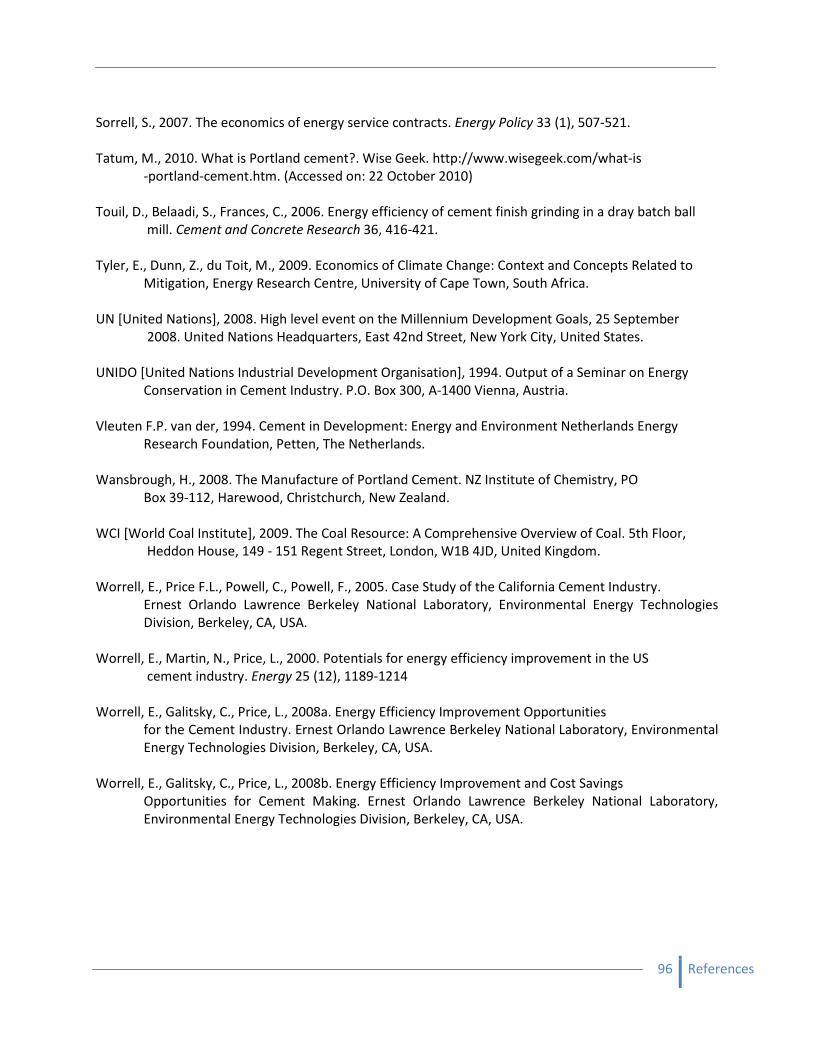
96 References


Tatum, M., 2010. What is Portland cement?. Wise Geek. http://www.wisegeek.com/what-is

-portland-cement.htm. (Accessed on: 22 October 2010)

Touil, D., Belaadi, S., Frances, C., 2006. Energy efficiency of cement finish grinding in a dray batch ball

mill. Cement and Concrete Research 36, 416-421.

Tyler, E., Dunn, Z., du Toit, M., 2009. Economics of Climate Change: Context and Concepts Related to

Mitigation, Energy Research Centre, University of Cape Town, South Africa.

UN [United Nations], 2008. High level event on the Millennium Development Goals, 25 September

2008. United Nations Headquarters, East 42nd Street, New York City, United States.

UNIDO [United Nations Industrial Development Organisation], 1994. Output of a Seminar on Energy

Conservation in Cement Industry. P.O. Box 300, A-1400 Vienna, Austria.

Vleuten F.P. van der, 1994. Cement in Development: Energy and Environment Netherlands Energy

Research Foundation, Petten, The Netherlands.

Wansbrough, H., 2008. The Manufacture of Portland Cement. NZ Institute of Chemistry, PO

Box 39-112, Harewood, Christchurch, New Zealand.

WCI [World Coal Institute], 2009. The Coal Resource: A Comprehensive Overview of Coal. 5th Floor,

Heddon House, 149 - 151 Regent Street, London, W1B 4JD, United Kingdom.

Worrell, E., Price F.L., Powell, C., Powell, F., 2005. Case Study of the California Cement Industry.

Ernest Orlando Lawrence Berkeley National Laboratory, Environmental Energy Technologies

Division, Berkeley, CA, USA.

Worrell, E., Martin, N., Price, L., 2000. Potentials for energy efficiency improvement in the US

cement industry. Energy 25 (12), 1189-1214

Worrell, E., Galitsky, C., Price, L., 2008a. Energy Efficiency Improvement Opportunities

for the Cement Industry. Ernest Orlando Lawrence Berkeley National Laboratory, Environmental

Energy Technologies Division, Berkeley, CA, USA.

Worrell, E., Galitsky, C., Price, L., 2008b. Energy Efficiency Improvement and Cost Savings

Opportunities for Cement Making. Ernest Orlando Lawrence Berkeley National Laboratory,


97 Appendix

APPENDIX A – QUESTIONNAIRE

Eskom DSM Feasibility Questionnaire for Cement Plants

General Date:

Name of plant:

Plant capacity:

Baseline (MWh/year):

Contact Person:

Contact Details: email:

Basic Plant Layout Please list the following

Number of crushers: ____

Number of raw mills: ____ Type: vertical roller mill / ball mill / hammer mill

/other (please specify) ___________________

Are the raw mills provided hot air from: a furnace / kiln waste gases / other yes / no

Type of transport system between raw mill and stock: mechanical /pneumatic.

. /other _____________________

Type of particle size separator following raw mill:

Type of pre-heater:

Number of kilns: _____ Type: ______ _

If more than one, are they fed by separate silos? yes / no

Do they feed into one set of silos? yes / no

If not, please explain layout_______________________________________

Type of clinker cooler: (example: grate cooler)

Number of cement mills:__ __ Type: vertical roller mill / ball mill /

roller press (crusher) /other (please specify)

Type of particle size separator following cement mill:

Do you prepare your kiln fuel on site, i.e. coal mills? yes / no

98 Appendix

Please draw a basic layout of the plant

SCADA Data

Does the SCADA display information on the:

Crushers yes / no

Raw mills yes / no

Silo levels -Raw meal yes / no

-Clinker yes / no

Kiln yes / no

Cement mills yes / no

Coal mills yes / no

What information does the SCADA log? (Example: electrical demand, flow rate)

Does it provide historic profiles?

It is possible to provide at least 3 months of SCADA data?

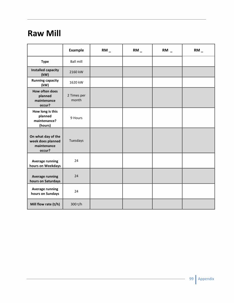
99 Appendix

Raw Mill

Example RM _ RM _ RM _ RM _

Type Ball mill

Installed capacity

(kW) 2160 kW

Running capacity

(kW) 1620 kW

How often does

planned

maintenance

occur?

2 Times per

month

How long is this

planned

maintenance?

(hours)

9 Hours

On what day of the

week does planned

maintenance

occur?

Tuesdays

Average running

hours on Weekdays

24

Average running

hours on Saturdays

24

Average running

hours on Sundays 24

Mill flow rate (t/h) 300 t/h

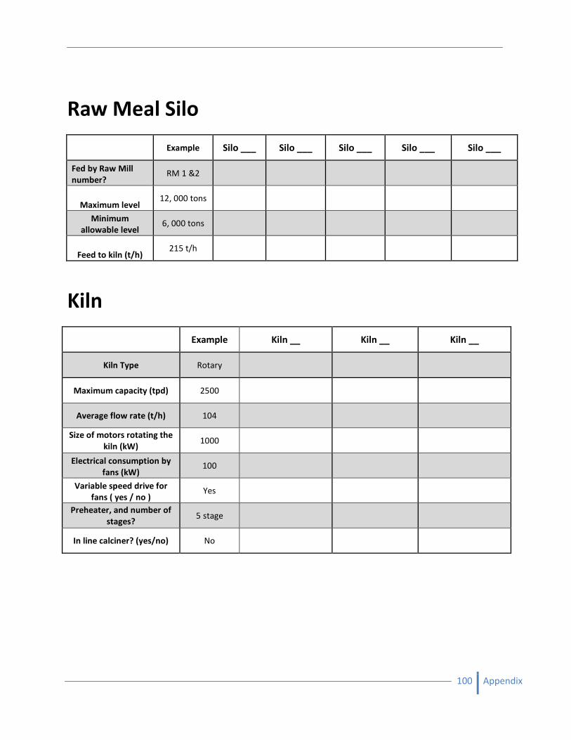
100 Appendix

Raw Meal Silo

Example Silo ___ Silo ___ Silo ___ Silo ___ Silo ___

Fed by Raw Mill

number? RM 1 &2

Maximum level 12, 000 tons

Minimum

allowable level 6, 000 tons

Feed to kiln (t/h) 215 t/h

Kiln

Example Kiln __ Kiln __ Kiln __

Kiln Type Rotary

Maximum capacity (tpd) 2500

Average flow rate (t/h) 104

Size of motors rotating the

kiln (kW) 1000

Electrical consumption by

fans (kW) 100

Variable speed drive for

fans ( yes / no ) Yes

Preheater, and number of

stages? 5 stage

In line calciner? (yes/no) No

101 Appendix

Finishing Mills

Clinker Silo

Example FM _ FM _ FM _ FM _

Type of mill Vertical roller mill

Installed capacity of mill

motor (kW) 1044 kW

Running capacity of mill

motor (kW) 783 kW

How often does planned

maintenance occur? 2 Times per month

How long is this planned

maintenance? (hours) 9 Hours

On what day of the week

does planned

maintenance occur?

Tuesday

Average running hours on

weekdays 24


Saturdays 24


Sundays 24

Mill flow rate (t/h) 350 t/h

Example Silo__ Silo __ Silo __ Silo __ Silo ___

Fed by Kiln

number? Kiln 1

Maximum level 12, 000 tons

Minimum

allowable level 6, 000 tons

Feeds into

finishing mill

number?

FM 1 & 2

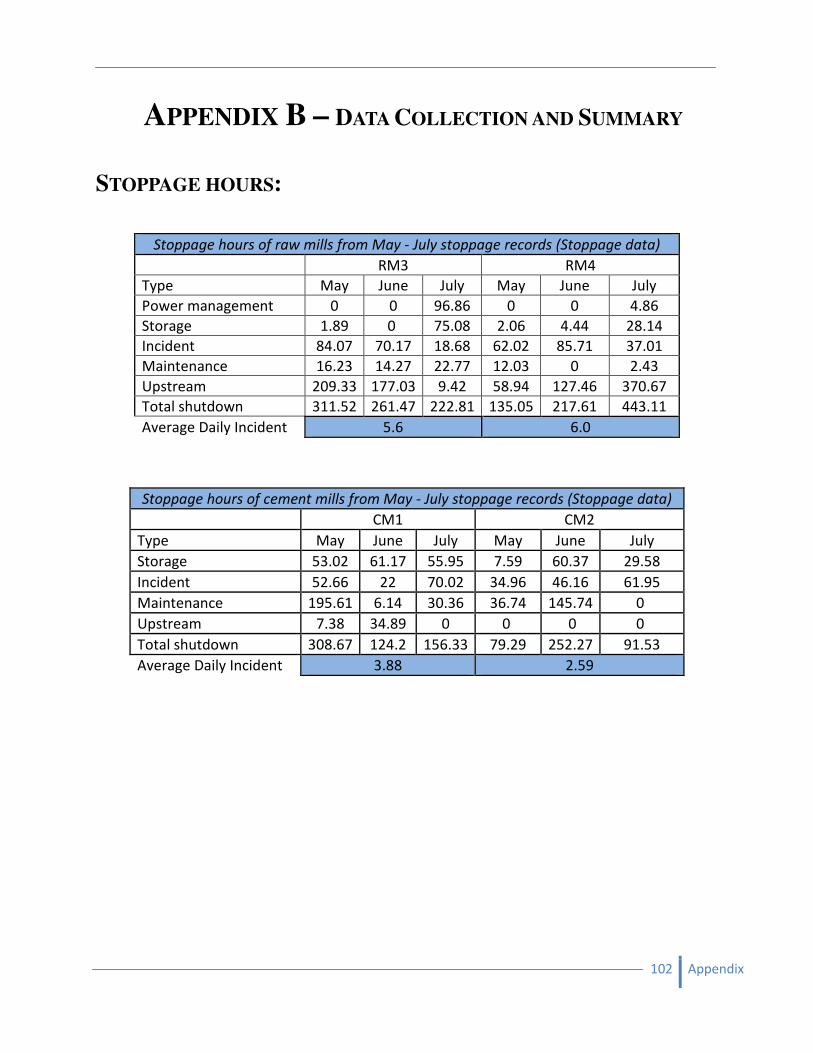
102 Appendix

APPENDIX B – DATA COLLECTION AND SUMMARY

STOPPAGE HOURS:

Stoppage hours of raw mills from May - July stoppage records (Stoppage data)

RM3 RM4

Type May June July May June July

Power management 0 0 96.86 0 0 4.86

Storage 1.89 0 75.08 2.06 4.44 28.14

Incident 84.07 70.17 18.68 62.02 85.71 37.01

Maintenance 16.23 14.27 22.77 12.03 0 2.43

Upstream 209.33 177.03 9.42 58.94 127.46 370.67

Total shutdown 311.52 261.47 222.81 135.05 217.61 443.11

Average Daily Incident 5.6 6.0

Stoppage hours of cement mills from May - July stoppage records (Stoppage data)

CM1 CM2

Type May June July May June July

Storage 53.02 61.17 55.95 7.59 60.37 29.58

Incident 52.66 22 70.02 34.96 46.16 61.95

Maintenance 195.61 6.14 30.36 36.74 145.74 0

Upstream 7.38 34.89 0 0 0 0

Total shutdown 308.67 124.2 156.33 79.29 252.27 91.53

Average Daily Incident 3.88 2.59

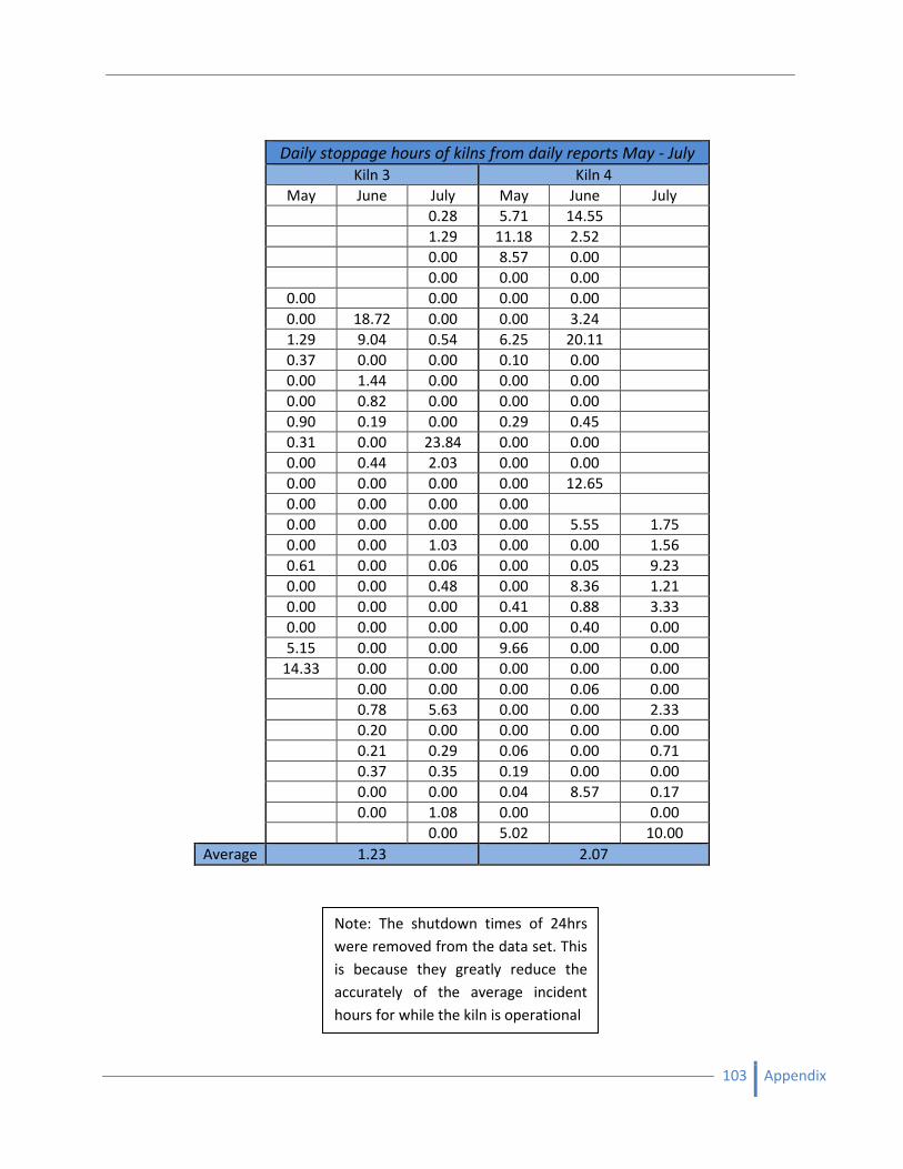
103 Appendix

Daily stoppage hours of kilns from daily reports May - July

Kiln 3 Kiln 4

May June July May June July

0.28 5.71 14.55

1.29 11.18 2.52

0.00 8.57 0.00

0.00 0.00 0.00

0.00

0.00 0.00 0.00

0.00 18.72 0.00 0.00 3.24

1.29 9.04 0.54 6.25 20.11

0.37 0.00 0.00 0.10 0.00

0.00 1.44 0.00 0.00 0.00

0.00 0.82 0.00 0.00 0.00

0.90 0.19 0.00 0.29 0.45

0.31 0.00 23.84 0.00 0.00

0.00 0.44 2.03 0.00 0.00

0.00 0.00 0.00 0.00 12.65

0.00 0.00 0.00 0.00

0.00 0.00 0.00 0.00 5.55 1.75

0.00 0.00 1.03 0.00 0.00 1.56

0.61 0.00 0.06 0.00 0.05 9.23

0.00 0.00 0.48 0.00 8.36 1.21

0.00 0.00 0.00 0.41 0.88 3.33

0.00 0.00 0.00 0.00 0.40 0.00

5.15 0.00 0.00 9.66 0.00 0.00

14.33 0.00 0.00 0.00 0.00 0.00

0.00 0.00 0.00 0.06 0.00

0.78 5.63 0.00 0.00 2.33

0.20 0.00 0.00 0.00 0.00

0.21 0.29 0.06 0.00 0.71

0.37 0.35 0.19 0.00 0.00

0.00 0.00 0.04 8.57 0.17

0.00 1.08 0.00

0.00

0.00 5.02

10.00

Average 1.23 2.07

Note: The shutdown times of 24hrs

were removed from the data set. This

is because they greatly reduce the

accurately of the average incident

hours for while the kiln is operational

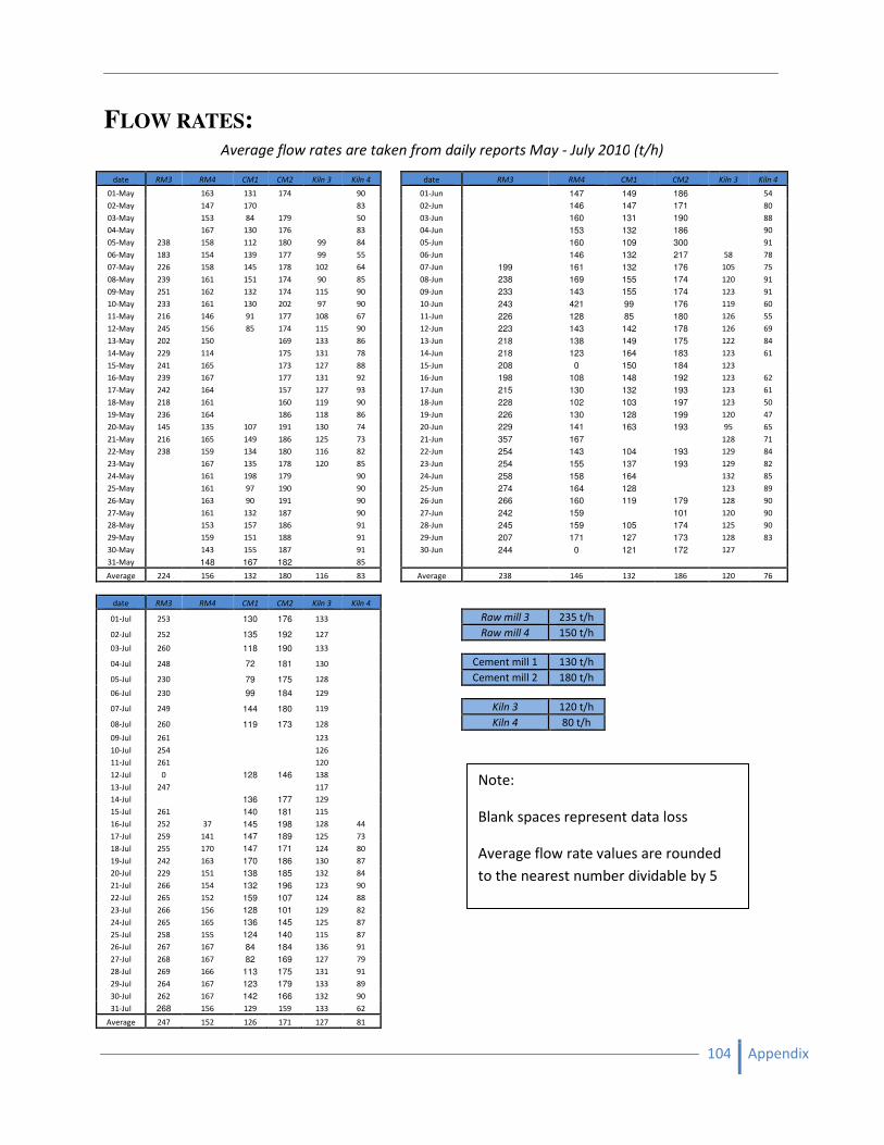
104 Appendix

FLOW RATES: Average flow rates are taken from daily reports May - July 2010 (t/h)

date RM3 RM4 CM1 CM2 Kiln 3 Kiln 4 date RM3 RM4 CM1 CM2 Kiln 3 Kiln 4

01-May 163 131 174 90 01-Jun 147 149 186 54

02-May 147 170 83 02-Jun 146 147 171 80

03-May 153 84 179 50 03-Jun 160 131 190 88

04-May 167 130 176 83 04-Jun 153 132 186 90

05-May 238 158 112 180 99 84 05-Jun 160 109 300 91

06-May 183 154 139 177 99 55 06-Jun 146 132 217 58 78

07-May 226 158 145 178 102 64 07-Jun 199 161 132 176 105 75

08-May 239 161 151 174 90 85 08-Jun 238 169 155 174 120 91

09-May 251 162 132 174 115 90 09-Jun 233 143 155 174 123 91

10-May 233 161 130 202 97 90 10-Jun 243 421 99 176 119 60

11-May 216 146 91 177 108 67 11-Jun 226 128 85 180 126 55

12-May 245 156 85 174 115 90 12-Jun 223 143 142 178 126 69

13-May 202 150 169 133 86 13-Jun 218 138 149 175 122 84

14-May 229 114 175 131 78 14-Jun 218 123 164 183 123 61

15-May 241 165 173 127 88 15-Jun 208 0 150 184 123

16-May 239 167 177 131 92 16-Jun 198 108 148 192 123 62

17-May 242 164 157 127 93 17-Jun 215 130 132 193 123 61

18-May 218 161 160 119 90 18-Jun 228 102 103 197 123 50

19-May 236 164 186 118 86 19-Jun 226 130 128 199 120 47

20-May 145 135 107 191 130 74 20-Jun 229 141 163 193 95 65

21-May 216 165 149 186 125 73 21-Jun 357 167 128 71

22-May 238 159 134 180 116 82 22-Jun 254 143 104 193 129 84

23-May 167 135 178 120 85 23-Jun 254 155 137 193 129 82

24-May 161 198 179 90 24-Jun 258 158 164 132 85

25-May 161 97 190 90 25-Jun 274 164 128 123 89

26-May 163 90 191 90 26-Jun 266 160 119 179 128 90

27-May 161 132 187 90 27-Jun 242 159 101 120 90

28-May 153 157 186 91 28-Jun 245 159 105 174 125 90

29-May 159 151 188 91 29-Jun 207 171 127 173 128 83

30-May 143 155 187 91 30-Jun 244 0 121 172 127

31-May 148 167 182 85

Average 224 156 132 180 116 83 Average 238 146 132 186 120 76

date RM3 RM4 CM1 CM2 Kiln 3 Kiln 4

01-Jul 253 130 176 133 Raw mill 3 235 t/h

02-Jul 252 135 192 127 Raw mill 4 150 t/h

03-Jul 260 118 190 133

04-Jul 248 72 181 130 Cement mill 1 130 t/h

05-Jul 230 79 175 128 Cement mill 2 180 t/h

06-Jul 230 99 184 129

07-Jul 249 144 180 119 Kiln 3 120 t/h

08-Jul 260 119 173 128 Kiln 4 80 t/h

09-Jul 261 123

10-Jul 254 126

11-Jul 261 120

12-Jul 0 128 146 138

13-Jul 247 117

14-Jul 136 177 129

15-Jul 261 140 181 115

16-Jul 252 37 145 198 128 44

17-Jul 259 141 147 189 125 73

18-Jul 255 170 147 171 124 80

19-Jul 242 163 170 186 130 87

20-Jul 229 151 138 185 132 84

21-Jul 266 154 132 196 123 90

22-Jul 265 152 159 107 124 88

23-Jul 266 156 128 101 129 82

24-Jul 265 165 136 145 125 87

25-Jul 258 155 124 140 115 87

26-Jul 267 167 84 184 136 91

27-Jul 268 167 82 169 127 79

28-Jul 269 166 113 175 131 91

29-Jul 264 167 123 179 133 89

30-Jul 262 167 142 166 132 90

31-Jul 268 156 129 159 133 62

Average 247 152 126 171 127 81

Note:

Blank spaces represent data loss

Average flow rate values are rounded

to the nearest number dividable by 5

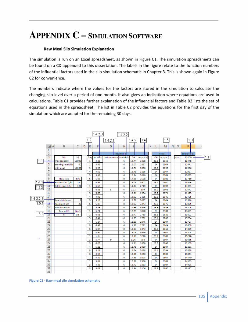
105 Appendix

APPENDIX C – SIMULATION SOFTWARE

Raw Meal Silo Simulation Explanation

The simulation is run on an Excel spreadsheet, as shown in Figure C1. The simulation spreadsheets can

be found on a CD appended to this dissertation. The labels in the figure relate to the function numbers

of the influential factors used in the silo simulation schematic in Chapter 3. This is shown again in Figure

C2 for convenience.

The numbers indicate where the values for the factors are stored in the simulation to calculate the

changing silo level over a period of one month. It also gives an indication where equations are used in

calculations. Table C1 provides further explanation of the influencial factors and Table B2 lists the set of

equations used in the spreadsheet. The list in Table C2 provides the equations for the first day of the

simulation which are adapted for the remaining 30 days.

Figure C1 - Raw meal silo simulation schematic

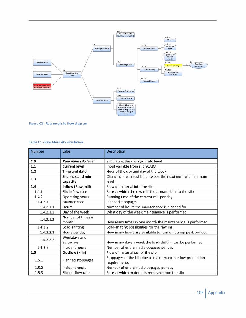
106 Appendix

Figure C2 - Raw meal silo flow diagram

Table C1 - Raw Meal Silo Simulation

Number Label Description

1.0 Raw meal silo level Simulating the change in silo level

1.1 Current level Input variable from silo SCADA

1.2 Time and date Hour of the day and day of the week

1.3 Silo max and min

capacity

Changing level must be between the maximum and minimum

level

1.4 Inflow (Raw mill) Flow of material into the silo

1.4.1 Silo inflow rate Rate at which the raw mill feeds material into the silo

1.4.2 Operating hours Running time of the cement mill per day

1.4.2.1 Maintenance Planned stoppages

1.4.2.1.1 Hours Number of hours the maintenance is planned for

1.4.2.1.2 Day of the week What day of the week maintenance is performed

1.4.2.1.3 Number of times a

month How many times in one month the maintenance is performed

1.4.2.2 Load-shifting Load-shifting possibilities for the raw mill

1.4.2.2.1 Hours per day How many hours are available to turn off during peak periods

1.4.2.2.2 Weekdays and

Saturdays How many days a week the load-shifting can be performed

1.4.2.3 Incident hours Number of unplanned stoppages per day

1.5 Outflow (Kiln) Flow of material out of the silo

1.5.1 Planned stoppages Stoppages of the kiln due to maintenance or low production

requirements

1.5.2 Incident hours Number of unplanned stoppages per day

1.5.3 Silo outflow rate Rate at which material is removed from the silo

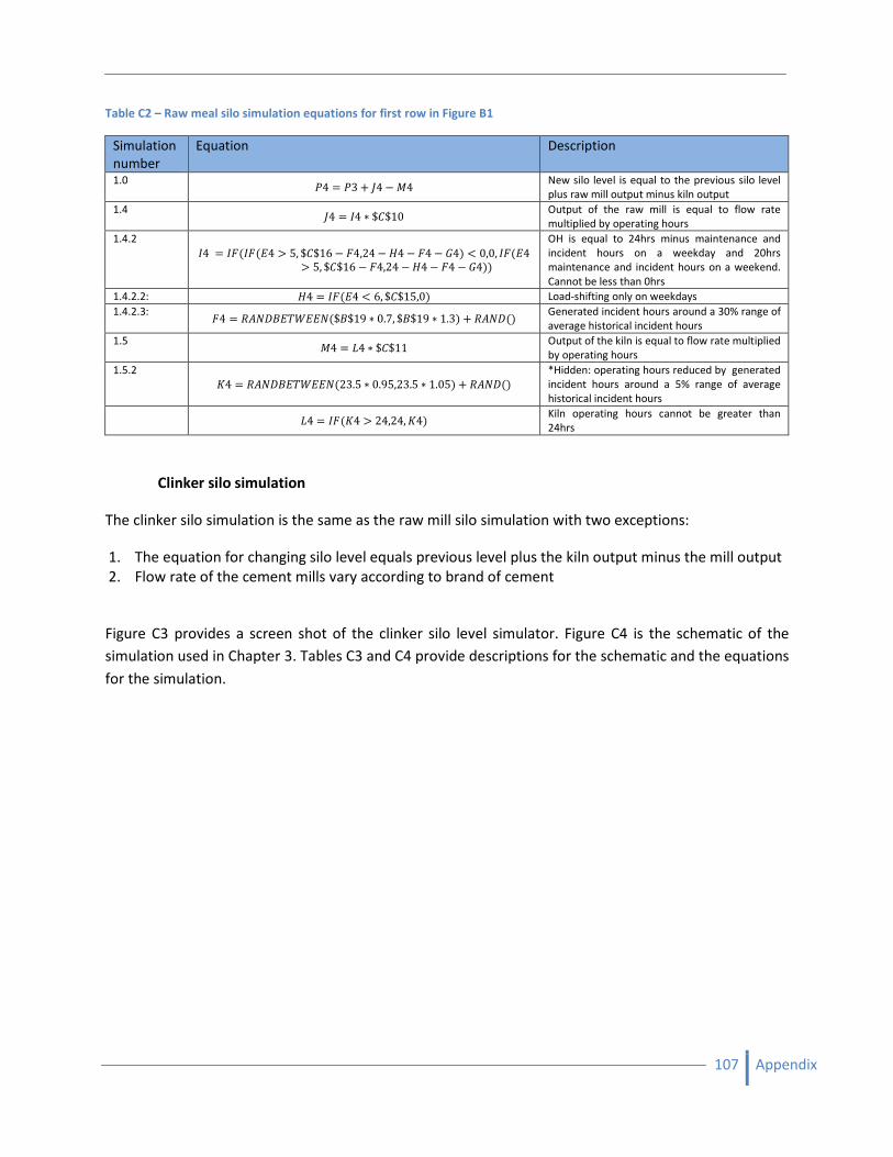
107 Appendix

Table C2 – Raw meal silo simulation equations for first row in Figure B1

Simulation

number

Equation Description

1.0 /4 /3 � 04 " 14

New silo level is equal to the previous silo level

plus raw mill output minus kiln output

1.4 04 24 3 $�$10

Output of the raw mill is equal to flow rate

multiplied by operating hours

1.4.2

24 26!26!)4 7 5, $�$16 " 64,24 " �4 " 64 " 94# : 0,0, 26!)47 5, $�$16 " 64,24 " �4 " 64 " 94##

OH is equal to 24hrs minus maintenance and

incident hours on a weekday and 20hrs

maintenance and incident hours on a weekend.

Cannot be less than 0hrs

1.4.2.2: �4 26!)4 : 6, $�$15,0# Load-shifting only on weekdays

1.4.2.3: 64 ;<=>?)@�))=!$?$19 3 0.7, $?$19 3 1.3# � ;<=>!#

Generated incident hours around a 30% range of

average historical incident hours

1.5 14 B4 3 $�$11

Output of the kiln is equal to flow rate multiplied

by operating hours

1.5.2

C4 ;<=>?)@�))=!23.5 3 0.95,23.5 3 1.05# � ;<=>!#

*Hidden: operating hours reduced by generated

incident hours around a 5% range of average

historical incident hours

B4 26!C4 7 24,24, C4#

Kiln operating hours cannot be greater than

24hrs

Clinker silo simulation

The clinker silo simulation is the same as the raw mill silo simulation with two exceptions:

1. The equation for changing silo level equals previous level plus the kiln output minus the mill output

2. Flow rate of the cement mills vary according to brand of cement

Figure C3 provides a screen shot of the clinker silo level simulator. Figure C4 is the schematic of the

simulation used in Chapter 3. Tables C3 and C4 provide descriptions for the schematic and the equations

for the simulation.

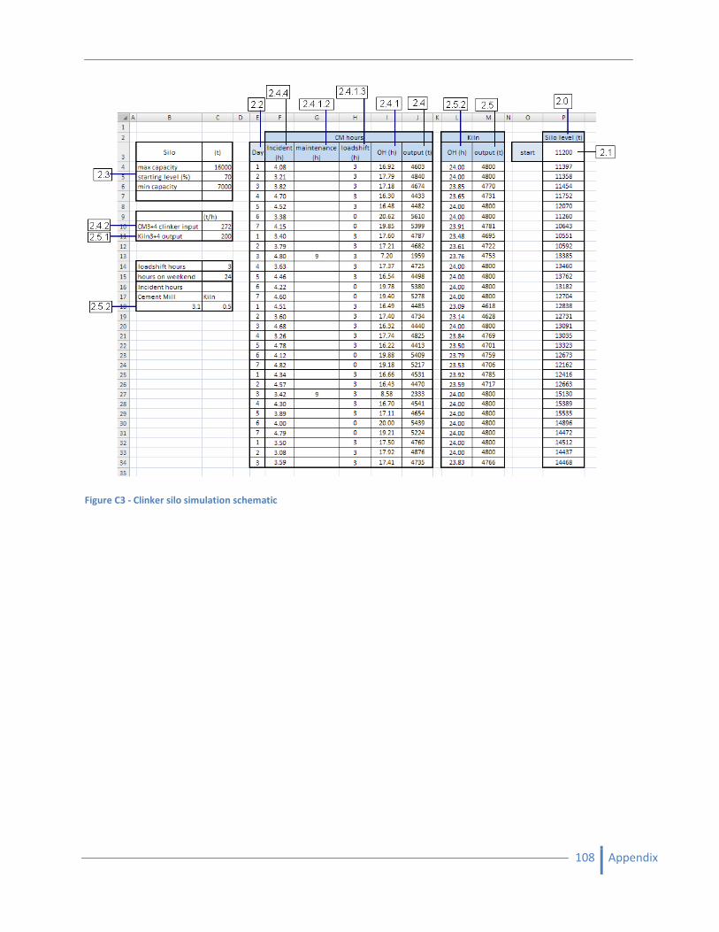
108 Appendix

Figure C3 - Clinker silo simulation schematic

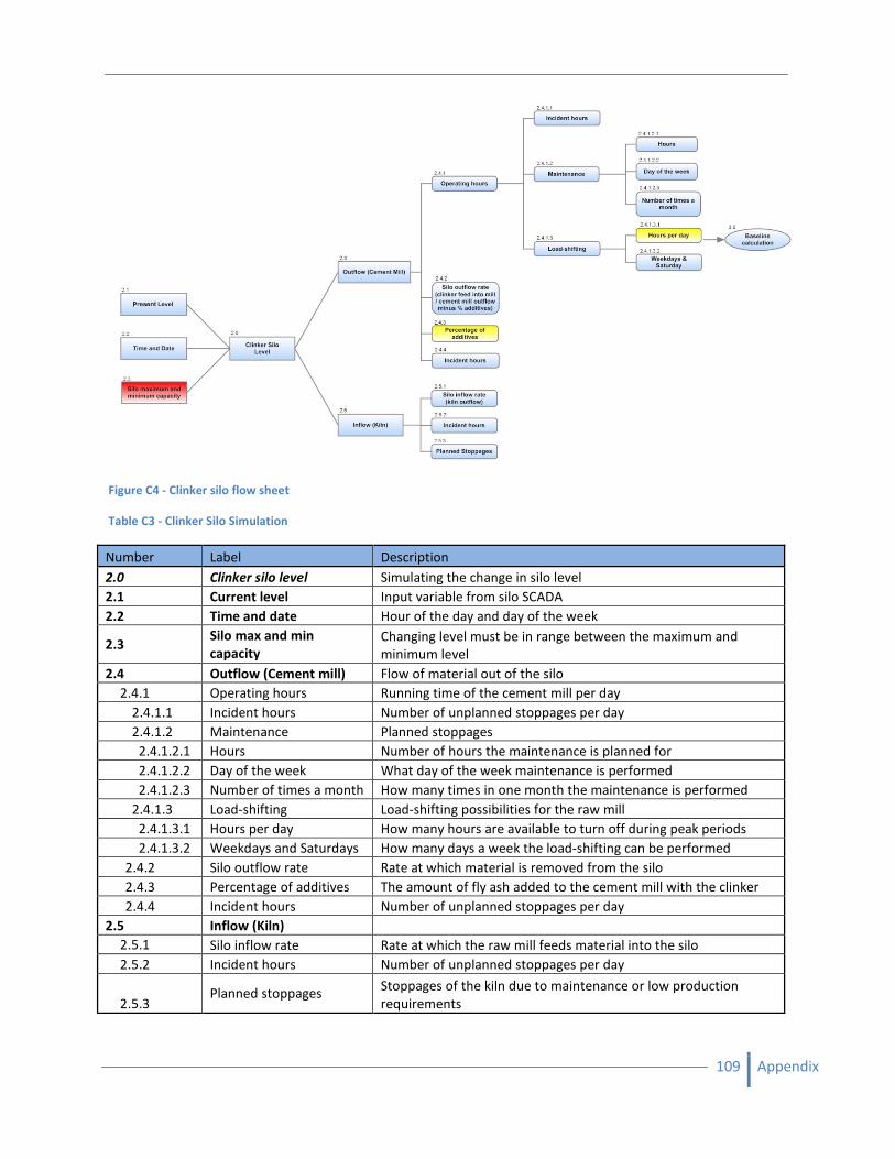
109 Appendix

Figure C4 - Clinker silo flow sheet

Table C3 - Clinker Silo Simulation


2.0 Clinker silo level Simulating the change in silo level

2.1 Current level Input variable from silo SCADA


2.3 Silo max and min

capacity

Changing level must be in range between the maximum and

minimum level

2.4 Outflow (Cement mill) Flow of material out of the silo

2.4.1 Operating hours Running time of the cement mill per day

2.4.1.1 Incident hours Number of unplanned stoppages per day

2.4.1.2 Maintenance Planned stoppages

2.4.1.2.1 Hours Number of hours the maintenance is planned for

2.4.1.2.2 Day of the week What day of the week maintenance is performed

2.4.1.2.3 Number of times a month How many times in one month the maintenance is performed

2.4.1.3 Load-shifting Load-shifting possibilities for the raw mill

2.4.1.3.1 Hours per day How many hours are available to turn off during peak periods

2.4.1.3.2 Weekdays and Saturdays How many days a week the load-shifting can be performed

2.4.2 Silo outflow rate Rate at which material is removed from the silo

2.4.3 Percentage of additives The amount of fly ash added to the cement mill with the clinker


2.5 Inflow (Kiln)

2.5.1 Silo inflow rate Rate at which the raw mill feeds material into the silo


2.5.3 Planned stoppages

Stoppages of the kiln due to maintenance or low production

requirements

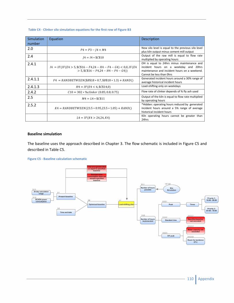
110 Appendix

Table C4 - Clinker silo simulation equations for the first row of Figure B3

Baseline simulation

The baseline uses the approach described in Chapter 3. The flow schematic is included in Figure C5 and

described in Table C5.

Figure C5 - Baseline calculation schematic

Simulation

number

Equation Description

2.0 /4 /3 " 04 � 14 New silo level is equal to the previous silo level

plus kiln output minus cement mill output

2.4 04 24 3 $�$10 Output of the raw mill is equal to flow rate

multiplied by operating hours

2.4.1 24 26!26!)4 7 5, $�$16 " 64,24 " �4 " 64 " 94# : 0,0, 26!)4

7 5, $�$16 " 64,24 " �4 " 64 " 94##

OH is equal to 24hrs minus maintenance and

incident hours on a weekday and 20hrs

maintenance and incident hours on a weekend.

Cannot be less than 0hrs

2.4.1.1 64 ;<=>?)@�))=!$?$18 3 0.7, $?$18 3 1.3# � ;<=>!# Generated incident hours around a 30% range of

average historical incident hours

2.4.1.3 �4 26!)4 : 6, $�$14,0# Load-shifting only on weekdays

2.4.2 �10 302 3 %��F�� !0.85; 0.8; 0.75# Flow rate of clinker depends of % fly ash used

2.5 14 B4 3 $�$11 Output of the kiln is equal to flow rate multiplied

by operating hours

2.5.2 C4 ;<=>?)@�))=!23.5 3 0.95,23.5 3 1.05# � ;<=>!#

*Hidden: operating hours reduced by generated

incident hours around a 5% range of average

historical incident hours

B4 26!C4 7 24,24, C4# Kiln operating hours cannot be greater than

24hrs

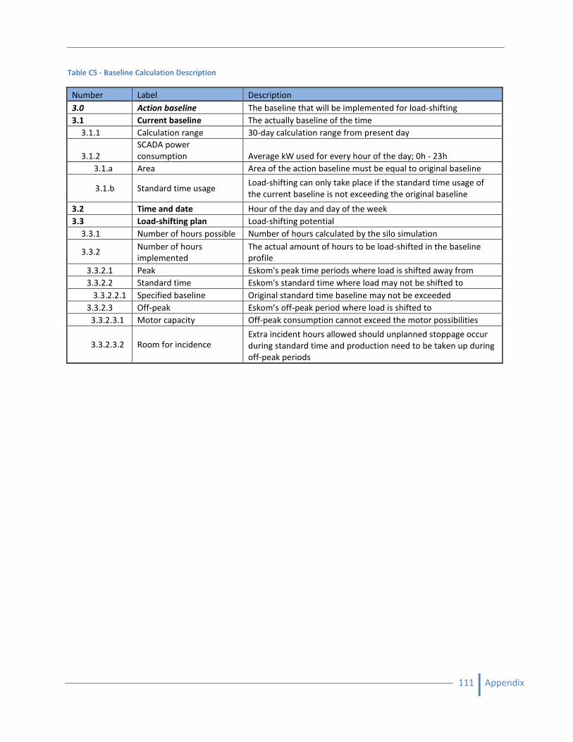
111 Appendix

Table C5 - Baseline Calculation Description


3.0 Action baseline The baseline that will be implemented for load-shifting

3.1 Current baseline The actually baseline of the time

3.1.1 Calculation range 30-day calculation range from present day

3.1.2

SCADA power

consumption Average kW used for every hour of the day; 0h - 23h

3.1.a Area Area of the action baseline must be equal to original baseline

3.1.b Standard time usage Load-shifting can only take place if the standard time usage of

the current baseline is not exceeding the original baseline


3.3 Load-shifting plan Load-shifting potential

3.3.1 Number of hours possible Number of hours calculated by the silo simulation

3.3.2 Number of hours

implemented

The actual amount of hours to be load-shifted in the baseline

profile

3.3.2.1 Peak Eskom's peak time periods where load is shifted away from

3.3.2.2 Standard time Eskom's standard time where load may not be shifted to

3.3.2.2.1 Specified baseline Original standard time baseline may not be exceeded

3.3.2.3 Off-peak Eskom’s off-peak period where load is shifted to

3.3.2.3.1 Motor capacity Off-peak consumption cannot exceed the motor possibilities

3.3.2.3.2 Room for incidence Extra incident hours allowed should unplanned stoppage occur

during standard time and production need to be taken up during

off-peak periods

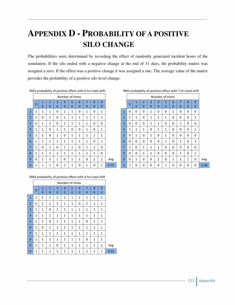
112 Appendix

APPENDIX D - PROBABILITY OF A POSITIVE

SILO CHANGE

The probabilities were determined by recording the effect of randomly generated incident hours of the

simulation. If the silo ended with a negative change at the end of 31 days, the probability matrix was

assigned a zero. If the effect was a positive change it was assigned a one. The average value of the matrix

provides the probability of a positive silo level change.

RM3 probability of positive effect with 6 hrs load-shift RM3 probability of positive effect with 7 hrs load-shift

Number of times

Number of times

0

1

0

2

0

3

0

4

0

5

0

6

0

7

0

8

0

9

0 0

1

0

2

0

3

0

4

0

5

0

6

0

7

0

8

0

9

0

1 1 1 1 0 1 1 0 1 0 1

1 0 0 0 1 0 0 1 0 0 0

2 1 0 1 0 1 1 1 1 1 1

2 1 1 0 1 1 1 0 0 0 1

3 0 1 1 0 1 1 1 1 0 0

3 0 0 0 1 1 0 0 1 0 0

4 1 1 0 1 1 0 0 1 0 1

4 1 1 1 0 1 1 0 0 0 1

5 1 1 0 1 0 1 1 1 1 1

5 0 1 0 1 0 1 0 0 0 0

6 1 1 1 1 1 1 1 1 0 1

6 0 0 0 0 0 1 0 1 0 1

7 1 0 1 0 1 1 0 1 1 0

7 1 0 1 1 1 0 0 0 0 0

8 1 1 1 1 1 1 1 1 1 0

8 0 0 1 1 0 0 0 1 0 1

9 0 1 1 1 0 1 1 0 1 1 Avg

9 0 1 0 0 1 0 1 1 1 0 Avg

0 1 1 1 0 1 1 0 1 0 1 0.73

0 1 0 0 0 0 1 0 0 0 0 0.38

RM4 probability of positive effect with 4 hrs load-shift

Number of times

0

1

0

2

0

3

0

4

0

5

0

6

0

7

0

8

0

9

0

1 1 1 1 1 1 1 1 1 1 1

2 0 1 1 1 1 1 0 1 1 1

3 1 1 0 1 1 1 1 1 1 1

4 1 1 1 1 1 1 1 1 1 1

5 1 1 0 1 1 1 1 0 1 1

6 1 0 1 1 1 1 1 1 1 1

7 1 1 1 1 1 1 1 1 1 1

8 1 1 1 1 1 1 1 0 1 1

9 1 1 1 0 1 1 1 1 1 1 Avg

0 1 1 1 1 1 1 1 1 1 1 0.92

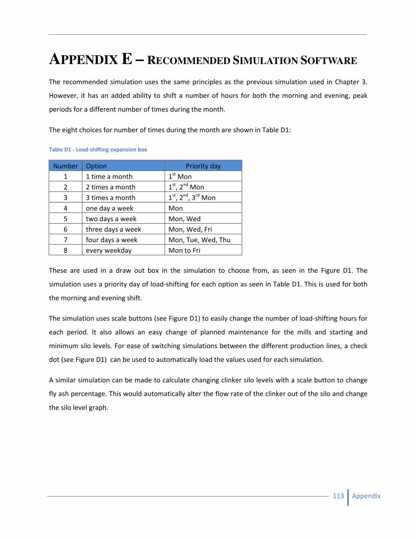
113 Appendix

APPENDIX E – RECOMMENDED SIMULATION SOFTWARE

The recommended simulation uses the same principles as the previous simulation used in Chapter 3.

However, it has an added ability to shift a number of hours for both the morning and evening, peak

periods for a different number of times during the month.

The eight choices for number of times during the month are shown in Table D1:

Table D1 - Load-shifting expansion box

Number Option Priority day

1 1 time a month 1st

Mon

2 2 times a month 1st

, 2nd

Mon

3 3 times a month 1st

, 2nd

, 3rd

Mon

4 one day a week Mon

5 two days a week Mon, Wed

6 three days a week Mon, Wed, Fri

7 four days a week Mon, Tue, Wed, Thu

8 every weekday Mon to Fri

These are used in a draw out box in the simulation to choose from, as seen in the Figure D1. The

simulation uses a priority day of load-shifting for each option as seen in Table D1. This is used for both

the morning and evening shift.

The simulation uses scale buttons (see Figure D1) to easily change the number of load-shifting hours for

each period. It also allows an easy change of planned maintenance for the mills and starting and

minimum silo levels. For ease of switching simulations between the different production lines, a check

dot (see Figure D1) can be used to automatically load the values used for each simulation.

A similar simulation can be made to calculate changing clinker silo levels with a scale button to change

fly ash percentage. This would automatically alter the flow rate of the clinker out of the silo and change

the silo level graph.

114 Appendix

Scale buttons

Total change in

silo level

Graph of the

changing silo

level

Automatic change between

clinker production lines

Figure D1 - Recommended simulation

Documents

Demand Side Management opportunities for a typical South