DEMAND SIDE MANAGEMENT:

LOAD PROFILE ANALYSIS FOR CAMPUS BUILDING

ROBIN TING FANG YUAN

A project report submitted in partial fulfilment of the

requirements for the award of Bachelor of Engineering

(Hons.) Electrical and Electronic Engineering

Faculty of Engineering and Science

Universiti Tunku Abdul Rahman

April 2013

ii

DECLARATION

I hereby declare that this project report is based on my original work except for

citations and quotations which have been duly acknowledged. I also declare that it

has not been previously and concurrently submitted for any other degree or award at

UTAR or other institutions.

Signature :

Name : Robin Ting Fang Yuan

ID No. : 09UEB06526

Date :

iii

APPROVAL FOR SUBMISSION

I certify that this project report entitled “DEMAND SIDE MANAGEMENT:

LOAD PROFILE ANALYSIS FOR CAMPUS BUILDING” was prepared by

ROBIN TING FANG YUAN has met the required standard for submission in

partial fulfilment of the requirements for the award of Bachelor of Engineering

(Hons.) Electrical and Electronic Engineering at Universiti Tunku Abdul Rahman.

Approved by,

Signature :

Supervisor : Mr. Chua Kein Huat

Date :

iv

The copyright of this report belongs to the author under the terms of the

copyright Act 1987 as qualified by Intellectual Property Policy of Universiti Tunku

Abdul Rahman. Due acknowledgement shall always be made of the use of any

material contained in, or derived from, this report.

© 2013, Robin Ting Fang Yuan. All right reserved.

v

Specially dedicated to

my beloved family,

supervisor Mr. Chua Kein Huat,

and partners Mr. Teo Teck Cheong, Mr. Khor Wei Peng

vi

ACKNOWLEDGEMENTS

I would like to express my utmost gratitude to my research supervisor, Mr. Chua

Kein Huat for his invaluable advice, guidance and his enormous patience throughout

the development of the research. Participation of various competitions under his

supervision had indeed sharpened my skills in my field of research.

In addition, I would also like to express my gratitude to my partners, Mr. Teo

Teck Cheong and Mr. Khor Wei Peng who had helped and worked alongside me to

bring the project into completion. It is without doubt that I have gained much

experiences from working with them.

Again, I own a big thank to my beloved family who had provided me both

physical and mental support from time to time. They gave me untiring support along

the progress, and it has been of great value to me in order to complete the final year

project. I am grateful to their help, courage and support.

Finally, I would like to thank everyone who had contributed to the successful

completion of this project.

vii

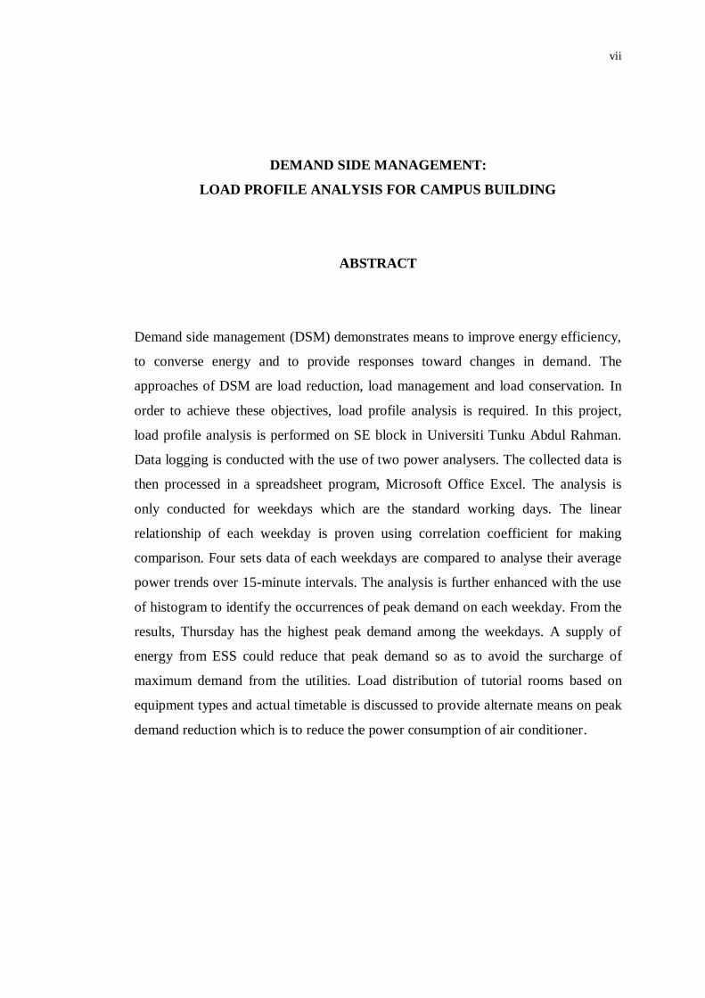
DEMAND SIDE MANAGEMENT:

LOAD PROFILE ANALYSIS FOR CAMPUS BUILDING

ABSTRACT

Demand side management (DSM) demonstrates means to improve energy efficiency,

to converse energy and to provide responses toward changes in demand. The

approaches of DSM are load reduction, load management and load conservation. In

order to achieve these objectives, load profile analysis is required. In this project,

load profile analysis is performed on SE block in Universiti Tunku Abdul Rahman.

Data logging is conducted with the use of two power analysers. The collected data is

then processed in a spreadsheet program, Microsoft Office Excel. The analysis is

only conducted for weekdays which are the standard working days. The linear

relationship of each weekday is proven using correlation coefficient for making

comparison. Four sets data of each weekdays are compared to analyse their average

power trends over 15-minute intervals. The analysis is further enhanced with the use

of histogram to identify the occurrences of peak demand on each weekday. From the

results, Thursday has the highest peak demand among the weekdays. A supply of

energy from ESS could reduce that peak demand so as to avoid the surcharge of

maximum demand from the utilities. Load distribution of tutorial rooms based on

equipment types and actual timetable is discussed to provide alternate means on peak

demand reduction which is to reduce the power consumption of air conditioner.

viii

TABLE OF CONTENTS

DECLARATION ii

APPROVAL FOR SUBMISSION iii

ACKNOWLEDGEMENTS vi

ABSTRACT vii

TABLE OF CONTENTS viii

LIST OF TABLES x

LIST OF FIGURES xi

LIST OF SYMBOLS / ABBREVIATIONS xiii

CHAPTER

1 INTRODUCTION 1

1.1 Background 1

1.2 Aims and Objectives 2

2 LITERATURE REVIEW 3

2.1 Demand Side Management 3

2.1.1 DSM Concepts 4

2.1.2 Types of DSM Approaches 7

2.2 Peak Demand 12

2.2.1 Energy Storage System 12

2.2.2 Prediction Model 13

2.3 Load Management 16

2.3.1 System Architecture 16

2.3.2 Types of Load 18

2.3.3 Load Distribution 19

ix

2.3.4 Load Scheduling 20

2.4 Adaptive Energy Forecasting 20

2.5 Demand Response Management 21

2.5.1 Information Integration Pipelines 22

2.5.2 Machine Learned Demand Forecasting Models 22

2.5.3 Information Diffusion Portal 23

3 METHODOLOGY 24

3.1 Site Investigation 24

3.2 Data Logging 25

3.3 Graph Tools 32

4 RESULTS AND DISCUSSION 34

4.1 Introduction 34

4.2 Total Power Consumption 34

4.3 Weekdays Analysis 35

4.3.1 Correlation Coefficient and Graph 35

4.4 Occurrence of Peak Demand 42

4.4.1 Use of Histogram 42

4.5 Load Distribution of Tutorial Rooms in SE Block 47

4.5.1 Types of Load 48

4.5.2 Power Consumption Based on Timetable 49

4.6 Load Shedding 49

4.6.1 Essential and Non-essential Loads 50

4.6.2 Alternate Mean to Reduce Peak Demand 50

4.7 Maximum Demand Surcharge 51

5 CONCLUSION AND RECOMMENDATIONS 53

5.1 Conclusion 53

5.2 Recommendations 54

REFERENCES 55

x

LIST OF TABLES

TABLE TITLE PAGE

3.1 Data Filtered According to Date 32

4.1 Correlation Coefficients of Mondays 35

4.2 Correlation Coefficients of Tuesdays 36

4.3 Correlation Coefficients of Wednesdays 37

4.4 Correlation Coefficients of Thursdays 38

4.5 Correlation Coefficients of Fridays 39

4.6 Correlation Coefficient of Weekdays 41

xi

LIST OF FIGURES

FIGURE TITLE PAGE

2.1 Three concept of DSM 5

2.2 Classic Forms of Load Levelling 9

2.3 Strategic Load Conservation 11

2.4 Strategic Load Growth 11

3.1 TES-3600 3P4W Power Analyser 25

3.2 Complete Setup of Data Logging Process 26

3.3 Clamping Onto Live Busbars 27

3.4 Two Power Analysers in Action 28

3.5 Close up View of Power Analyser 29

3.6 Graphical User Interface of Power Analyser 30

3.7 Status of Internal Memory 31

4.1 Average Power over 15-Minute Intervals on

Mondays 36

4.2 Average Power over 15-Minute Intervals on

Tuesdays 37

4.3 Average Power over 15-Minute Intervals on

Wednesdays 38

4.4 Average Power over 15-Minute Intervals on

Thursdays 39

4.5 Average Power over 15-Minute Intervals on

Fridays 40

xii

4.6 Average Powers over 15-Minute Intervals on

Weekdays 42

4.7 Histogram of Monday 43

4.8 Histogram of Tuesday 44

4.9 Histogram of Wednesday 44

4.10 Histogram of Thursday 45

4.11 Histogram of Friday 45

4.12 Occurrence Frequency of Power Consumption on

Weekdays 47

4.13 Load Distribution of Tutorial Rooms 48

4.14 Total Power Consumption of Tutorial Rooms on

Weekdays 49

xiii

LIST OF SYMBOLS / ABBREVIATIONS

kWh kilowatts-hours

DSM demand side management

DG distributed generation

ESS energy storage system

EE energy efficiency

EC energy conversation

DR demand response

BESS battery energy storage system

SVR support vector regression

LS-SVR least squares support vector regression

ANN artificial neural network

AC admission control

LB load balancer

LF load forecaster

DRM demand response manager

HVAC heating, ventilation and air conditioning

GUI graphical user interface

TKWh total power consumption

MD maximum demand

1

1 INTRODUCTION

1.1 Background

The ever increasing electricity bills due to poor energy management has raised a

concern among consumers who wish to cut down the electricity cost yet maintaining

the productivity. It is rather crucial to identify the possible causes and to tackle them

specifically to achieve desired results. There are more and more methods surfacing in

the market nowadays on how to study the behaviour of energy usage so to implement

efficient and effective solutions. It is no longer an issue of consumers whereby the

utilities come into play to work together with customers in executing the best

possible way to maintain power quality and stability.

One of the plausible and exciting methods will be demand side management

(DSM). It applies largely to the energy usage in order to bring a significant reduction

of cost to energy users. Demand side management provides opportunities to reduce

energy demand. There are many low cost or even no cost approaches that most

companies or individuals could learn to apply within a short period or long period, if

good practices of energy management. Several case studies shows the promising

potential of demand side management on saving costs and mitigating other power

issues around the globe. Two DSM case studies are drawn below for reference, one

from the United States and one from the Sultanate of Oman.

DSM programmes has been taken part by 459 large electricity utilities in the

United States in 1999. 50.6 billion kilowatt hours (kWh) of energy generation by the

large utilities was saved by these programme. This represented 1.5 % of the annual

electricity sales of that year. Moreover, New York shows great potential in reducing

demand by 1,300 MW in 2002 through DSM programmes. The amount is enough to

supply power to 1.3 million homes (Cogeneration Technologies, n.d.).

2

By 2012, the electrical energy demands in Sultanate of Oman are expected to

increase by about 60 % due to its fast growth in industrialization and country’s multi-

dimensional expansion activities. It has become vital for the government to look into

the mutual benefit of both utility and the customer by regulating the energy demands

and drafting suitable policies under DSM. A recommendation and implementation of

suitable policies to regulate energy demands would result a total annual energy

saving of 25.6% and a cost saving of $138,447 (Venkateswara, Parmal and Yousif,

2011).

1.2 Aims and Objectives

This project aims to integrate the application of demand side management to

university campus buildings. The main objective of this project is to undertake a load

profile analysis for a building in University Tunku Abdul Rahman, namely SE Block

and make analysis on how energy costs could be reduced. To examine the possibility

of the application of even load distribution and scheduling at reducing electricity

bills and thus avoiding the maximum demand penalty from energy supplier.

The key elements of load profile analysis comprised of the following:

1) To identify the energy consuming unit;

2) To estimate the quantity of energy consumed by each unit;

3) To analyse energy consumption patterns;

4) To identify energy savings opportunities;

5) To recommend conservation measures

3

CHAPTER 2

2 LITERATURE REVIEW

2.1 Demand Side Management

Demand side management (DSM) has been regarded as means of reducing peak

electricity demands so that utilities can delay the expansion of supply capacity. A

concept deals with energy efficiency measures that adjust and reduce energy demand

of end users. It introduces peak demand management which does not necessarily cut

down total energy consumption but shed loads to achieve optimum energy demands.

The adjustment applies not only to electricity loads but also to demands of all types

of energy. The clear benefit here is reduced energy costs for a given output.

Nowadays, it has become essential to access power in an efficient and

effective manner in order to save on cost. Demand side management is said to play

an important role in delaying high investment costs in generation, transmission and

distribution of power while still providing various practical benefits such as

mitigating electrical system outbreaks, reducing system blackouts and increasing

system reliability. Managing energy demands can substantially reduce dependency of

expensive fuels import, reduce high energy prices and reduce harmful environmental

impacts. All these in combination help to bring significant energy cost benefits.

4

Energy demands at wherever places can easily hit the peak load consumption

without prior load management. This can tell when electricity bill each months is

surcharged with an additional cost of maximum demand. It could be seen as a form

of penalty that could have easily been avoided if the exact figure of load

consumption is known. The two types of maximum demand surcharges are during

peak period and off peak period according to the pricing and tariff by Tenaga

Nasional Berhad.

On the other hand, DSM is greatly promoted with aims to provide cost

reduction, social and environmental improvement and network and reliability issues.

To save on the cost, DSM has introduced resources planning to reduce overall energy

demands so to reduce cost. Less energy consumption leads to a cleaner environment

because greenhouse gas emission and other environmental issues are reduced.

Reduction in energy demands improves power system reliability in the immediate

term. It also defers the need to upgrade power system which will save costs and

maintain the reliability (Palensky and Dietrich, 2011).

2.1.1 DSM Concepts

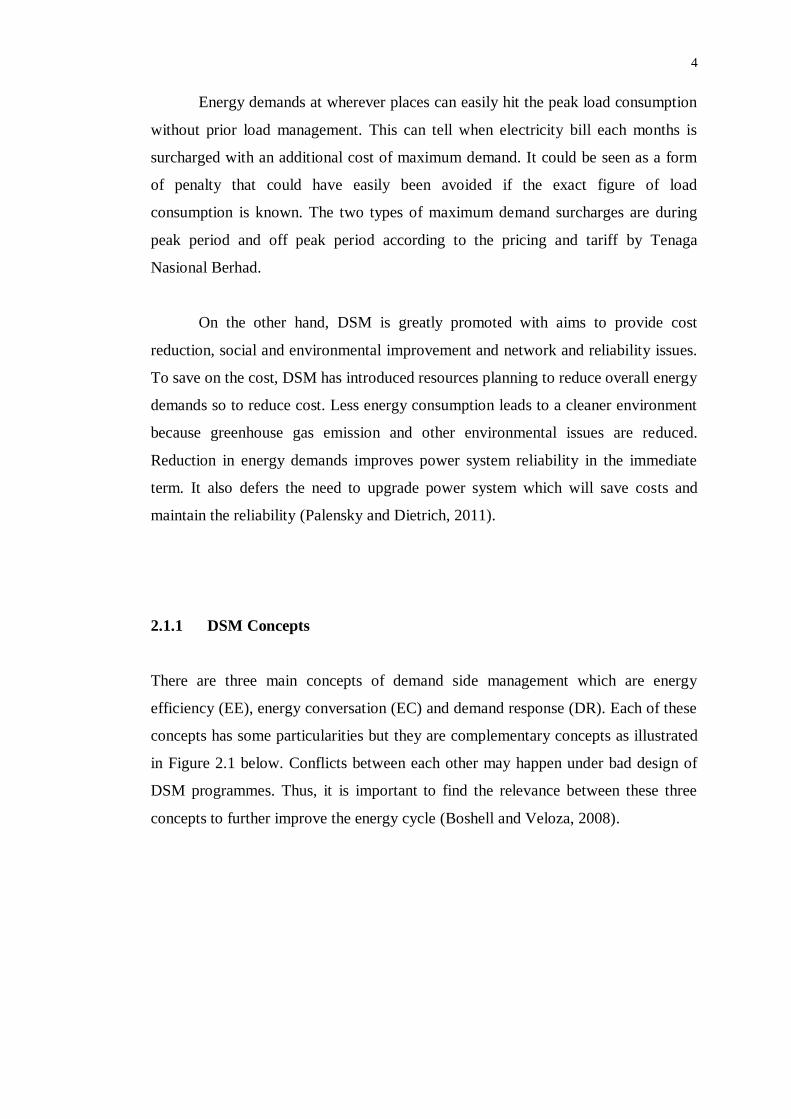
There are three main concepts of demand side management which are energy

efficiency (EE), energy conversation (EC) and demand response (DR). Each of these

concepts has some particularities but they are complementary concepts as illustrated

in Figure 2.1 below. Conflicts between each other may happen under bad design of

DSM programmes. Thus, it is important to find the relevance between these three

concepts to further improve the energy cycle (Boshell and Veloza, 2008).

5

Figure 2.1: Three concept of DSM

In simpler terms, energy efficiency is related to solutions from technological

advancements, whilst energy conversation is to achieve energy-saving through the

study of consumer’s behaviour, and finally demand response is based on the market

demand on electricity and its changeable price. Since they are complementary and

relevant to save energy, it is essential to promote adequate energy management

programmes within an electricity liberalized community.

2.1.1.1 Energy Efficiency

Energy efficiency are introduced to eliminate energy losses in existing power system

through the permanent installation of energy efficient technologies. The importance

of energy efficiency is to reduce energy usage and not to compromise on the level of

service provided.

6

Several approaches are promoted for better energy efficiency. It could be the

replacement of incandescent light bulbs with compact fluorescent bulbs, the

implementation of variable speed air conditioners that cool buildings using less

energy than typical air conditioners or the maintenance on leaky compressed air

networks.

2.1.1.2 Energy Conversation

Energy conversation promotes behavioural changes to use less resources in order to

achieve energy-saving. The effect could be for a short term or may last for a long

term as daily habits. It is a gradual change on the side of consumer’s behaviours to

integrate an energy-saving lifestyle. More resources and energy could be conserved

in the process and they could then be put into greater use in future.

It could a simple act like increasing cooling temperature from 16°C to 24°C

for air conditioning system, waiting until the washing machine is fully loaded with

clothes and wearing light clothes during hot seasons to cut down the use of air

conditioners.

2.1.1.3 Demand Response

Demand response is often related to current market of electricity and its price.

Consumers are exposed with two strategies which are load management and load

shifting. Total loads are curtailed in response to signals received from the service

provider to avoid surcharges. It is also possible to shift loads from peak periods to

another time periods for a lower tariff of electricity cost.

7

Dynamic pricing is a new approach to load management which will induce

customers to cut down power consumption at specific times or shift loads to other

time periods, usually when the energy is at its highest price. Customers are made

aware of their power consumptions and the related charges through demand response

initiatives of information and communication technologies.

2.1.2 Types of DSM Approaches

2.1.2.1 Load Reduction

It aims to reduce demands through efficient processes, buildings and equipment. It

mainly revolves around energy saving tips for the existing so-called household

appliances. Most of them can be implemented at little or no cost, but some requires a

significant capital investment due to their particular connection to industrial and

commercial businesses.

A common practice to produce hot water and water with the use of relevant

technology is perhaps a major activity for most enterprises. Inefficient steam systems

and boiler operation represent a significant source of energy losses. Poor

maintenance as well as poor original design could also incur significant losses.

Performance improvement steps which are practical and at low cost are often

considered. Adequate controls to adjust the configuration are required to routinely

monitor conditions of the systems in order to keep the efficiency as high as possible.

Lighting often consumes 10% or more of electricity in industrial plant or 50%

or more in commercial buildings. A great opportunity to save is possible in lighting

system. The improvement could either be applied to a lesser or greater extent to the

domestic sector. The common practice to improve lighting efficiency is to replace the

existing type with energy efficient fluorescent tubes, CFL, and other low energy light

sources. Other alternative is to consider using energy efficient electronic ballasts.

The implementation of lighting control can set appropriate luminosity for different

8

parts of the area. Perhaps, cleaning of fluorescent tube on a regular basic is essential

to maintain the luminosity it can provide.

However, lighting system does not consume as much electricity as air

conditioning system and laboratory machineries when referring to the university

setting. In fact, major portion of electricity is spent on air conditioning system and

followed by laboratory machineries. The energy saving tips for previous listed two

items rely much on regular maintenances and services to keep them performed at

high efficiency at all times. Laboratories machineries consist mostly motors and

drive systems. These high power motors should be used properly and only run when

needed. Electronic variable speed controls can be used where motor loads are

variable in normal operation. Checking power factor regularly to ensure optimum

operation of those machineries (REEEP/UNIDO Training Package, n.d.).

2.1.2.2 Load Management

Reducing demand at peak time and peak rates and varying the load pattern would

definitely help in reducing electricity costs while having evenly distributed loads

across the network. End-users can apply load management to achieve the

redistribution of the demands and time of electricity usage under the influence of

electricity suppliers. Normal production and operation generally will not be affected

under the execution of load management programmes while having the utility to

achieve a modified load curve. Load levelling, load control and tariff incentives and

penalties are the types of load management techniques involved.

2.1.2.2.1 Load Levelling

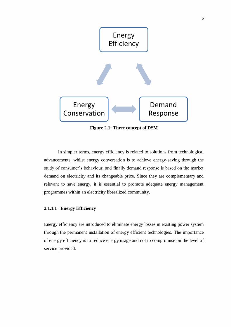
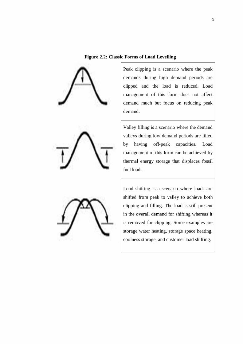
Load levelling helps to regulate the base load of current generation without the need

for additional supply to meet the peak demand periods. Table 2.2 below shows the

classic forms of load levelling (Alyasin, et al., 1994).

9

Figure 2.2: Classic Forms of Load Levelling

Peak clipping is a scenario where the peak

demands during high demand periods are

clipped and the load is reduced. Load

management of this form does not affect

demand much but focus on reducing peak

demand.

Valley filling is a scenario where the demand

valleys during low demand periods are filled

by having off-peak capacities. Load

management of this form can be achieved by

thermal energy storage that displaces fossil

fuel loads.

Load shifting is a scenario where loads are

shifted from peak to valley to achieve both

clipping and filling. The load is still present

in the overall demand for shifting whereas it

is removed for clipping. Some examples are

storage water heating, storage space heating,

coolness storage, and customer load shifting.

10

2.1.2.2.2 Load Control

Load control is where loads such as lighting, ventilation, heating and cooling can be

switched on or off remotely depending on the situations. In a situation when the

supply is cut off by the utility, customers may need back-up generators or energy

storage system to face the electricity cut-off. Generally, they may have asked for a

special rate from the utility on the interruption. Moreover, on-site generators could

be called by the utilities to meet peak demand on the gird. This creates alternate

means to deal with the peak demand and to reduce the heavy burden at utility side.

Rolling blackouts is one of the many ways to cut down demand when the

demand exceeds the capacity. It is commonly practised in energy distribution

industry. By definition, rolling blackouts are the systematic cutting off of supply to

areas within a supplied region such that each area takes turns to lose supply. Prior

announcements or schedule notices could be made so that companies and homes can

plan their energy usage for that period. Effective communication is essential at both

sides to prevent mass confusion, lost production and even lost goods.

2.1.2.2.3 Tariff Penalties

Utilities could use tariff penalties to warn customers a certain energy usage pattern at

certain times to avoid the penalties. These include:

1. Maximum demand charges

Utilities have different charges for maximum demand. Higher maximum

demand charges would encourage a user to distribute loads in an even fashion

to avoid the penalty.

2. Power factor charges

Surcharges are applied if users are having power factors below a fixed

threshold of 0.85.

11

2.1.2.3 Load Conservation and Growth

Since environmental health is at great dire, inevitably the world is turning to

sustainable green solutions to conserve energy. Conventional methods which cause

greenhouse gases emission will eventually be replaced with electric products which

offer a switch from the use of polluting fuels to non-polluting electricity without

sacrificing the performance factor.

Load conservation programmes are generally utility-stimulated and directed

at consumption of end users. The programme is further enhanced by having a

reduction in loads, a change in the pattern of energy usage and an improvement on

efficiency of electrical appliances. Strategic conservation shown in Figure 2.3 below

is the change of load shape which results from programmes stimulated by utilities

directed at consumption of end users.

Figure 2.3: Strategic Load Conservation

Implementation of load growth programmes aims to improve customer

productivity and environmental compliance while increasing the sale of power for

the utilities. The market share of the utility increases and this enables an ability to

increase peaks and fill valleys. These programmes can often divert unsustainable

energy practices to better and more efficient practices such as the reduction of the

use of fossil fuels and raw materials. Strategic load growth shown in Figure 2.4

below is the change of load shape which refers to a general sales increase beyond the

valley filling.

Figure 2.4: Strategic Load Growth

12

2.2 Peak Demand

Peak demand is the highest power consumption at any given time. The expensive

infrastructural costs of extra power plants would be deferred with a reduction in peak

demand. At the same time, this would help lower the generation cost and electricity

prices. Energy storage system and a prediction model are proposed to achieve peak

demand reduction.

Energy storage system offers a wide range of application besides the

reduction of peak demand. It is largely used with distributed generation to store and

dispatch energy. The latter one require an accurate prediction of peak and mean

demand. The use of machine learning techniques are investigated to develop

predictive model that uses observable characteristics such as past load values, day,

time, season and weather associated with their occurrence, to predict the next peak

demand. It is essential to model the expected behaviour of loads accurately in order

to allow such system to operate efficiently.

2.2.1 Energy Storage System

Energy storage system (ESS) could be charged or discharged intelligently if the peak

demand can be predicted, leading to a better power utilisation. Energy storage aims

to reduce peak load by allowing the building to consume stored energy during peak

hours. With the use of peak load prediction model, energy can be used in a way that

serves the interests of grid while maximizing the consumer’s comfort.

Electricity generation based on renewable sources has become increasingly

important for the sake of a greener and cleaner environment. Distributed generation

(DG) is generally site generation that is closer to demands. There have been several

DG settings put into operation around the globe in recent years. They include wind

turbines, solar cells, and hydro plants. The dependency of DG could be inconsistent

due to the unpredictable nature of the sources. Therefore, ESS is used in DG to store

energy directly from the generation and dispatch energy to support the grid whenever

necessary (Choi, Tseng, Vilathgamuwa and Nguyen, 2008).

13

One common ESS would be battery energy storage system (BESS). A battery

uses chemical reaction of its electrochemical components to store electrical energy.

When charging a battery, the energy is stored in chemical form due to reactions in

the compounds. On the other hand, reverse chemical reactions can supply electricity

out of the battery and back to the grid upon demand. The highlight of a battery would

be its quick response as some batteries can respond to load changes in about 20ms.

Depending on the types of electrochemical used and the frequency of cycle, the

efficiency of batteries is in the range of 60 to 80% (Schainker, 2004).

2.2.2 Prediction Model

Singh, Peter and Daniel (2012) describes and employs regression based prediction.

Different properties that drive peak load are studied through a set of five relevant

features of each measured peak load value . Subsections below describe their

definition, physical meaning and motivation.

2.2.2.1 Time of Day ( )

In a campus, occupancy and activities of consumer typically follows an underlying

routine. For instance, students attend classes from the morning to the evening, use air

conditioning and lighting throughout the sessions. This intrinsic pattern is likely to

repeat across different days. In relation to hourly peak load , time of day ( ) is

defined as a feature, where

14

2.2.2.2 Day of week ( )

Consumer occupancy and activity patterns remain active on weekdays (Monday to

Friday) as compared to weekend days (Saturday and Sunday). Thus, in addition to

considering the time t of the peak load yt, the day of the week ( ) is defined as a

feature, where .

2.2.2.3 Ambient temperature ( )

Energy consumption is greatly affected by weather and seasonality. It has been used

to model it. This is due to the use of air conditioners in hot weather. Extending this

approach, is defined as the average ambient air temperature, and is used as a

feature for the hour because is not noticeable until the hour.

2.2.2.4 Variance ( )

Most devices undergo a cycle of different modes of operation and varying

consumption. Examples include using several types of machinery together. These

different modes of operation result a large variation in the total load when in

operation. Thus, the variance of measured load values is defined during the

hour as a feature of for hour to capture consumer activity.

15

2.2.2.5 Last peak load ( )

The activity period of a user normally spans across hours. If the peak load of

previous hour was high, a consumer is more likely to cause the hourly peak load to

be high due to his activity. This is supported by the dataset which shows a high

correlation of 0:52 between consecutive hours’ peak load values.

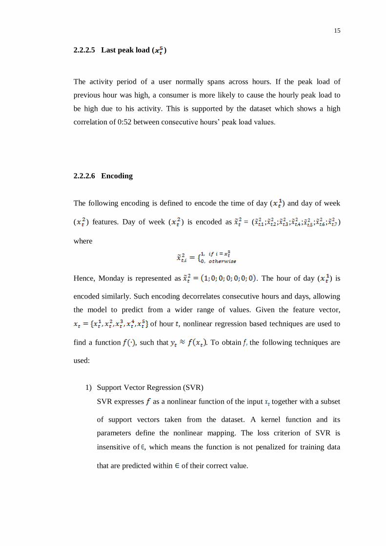
2.2.2.6 Encoding

The following encoding is defined to encode the time of day ( ) and day of week

( ) features. Day of week ( ) is encoded as = ( ; ; ; ; ; ; )

where

Hence, Monday is represented as . The hour of day ( ) is

encoded similarly. Such encoding decorrelates consecutive hours and days, allowing

the model to predict from a wider range of values. Given the feature vector,

of hour , nonlinear regression based techniques are used to

find a function , such that . To obtain the following techniques are

used:

1) Support Vector Regression (SVR)

SVR expresses as a nonlinear function of the input together with a subset

of support vectors taken from the dataset. A kernel function and its

parameters define the nonlinear mapping. The loss criterion of SVR is

insensitive of , which means the function is not penalized for training data

that are predicted within of their correct value.

16

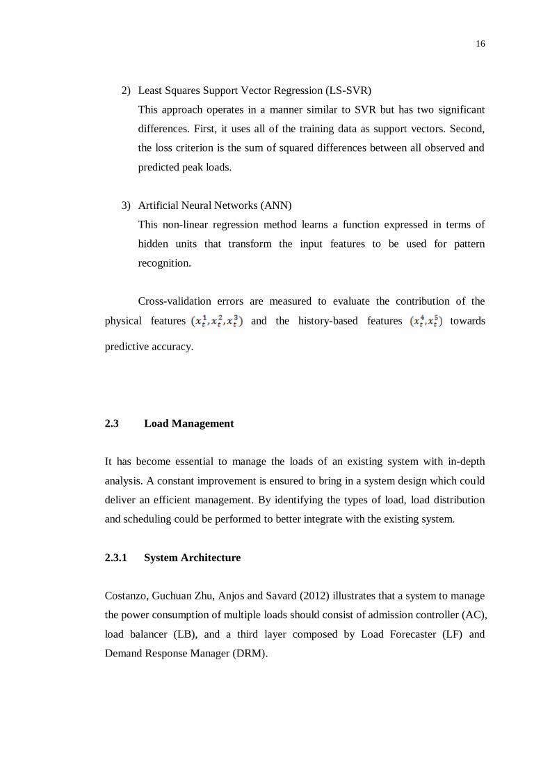
2) Least Squares Support Vector Regression (LS-SVR)

This approach operates in a manner similar to SVR but has two significant

differences. First, it uses all of the training data as support vectors. Second,

the loss criterion is the sum of squared differences between all observed and

predicted peak loads.

3) Artificial Neural Networks (ANN)

This non-linear regression method learns a function expressed in terms of

hidden units that transform the input features to be used for pattern

recognition.

Cross-validation errors are measured to evaluate the contribution of the

physical features and the history-based features towards

predictive accuracy.

2.3 Load Management

It has become essential to manage the loads of an existing system with in-depth

analysis. A constant improvement is ensured to bring in a system design which could

deliver an efficient management. By identifying the types of load, load distribution

and scheduling could be performed to better integrate with the existing system.

2.3.1 System Architecture

Costanzo, Guchuan Zhu, Anjos and Savard (2012) illustrates that a system to manage

the power consumption of multiple loads should consist of admission controller (AC),

load balancer (LB), and a third layer composed by Load Forecaster (LF) and

Demand Response Manager (DRM).

17

The bottom layer is the AC applying real-time load control by interacting

with physical equipment. The middle layer is the LB coordinating admission control

and demand response management using optimization that distribute the load to

reduce the operational cost while considering capacity limits defined by DRM and

operational constraints specified for each device. The LB provides also the DRM

with information such as rejection rate and capacity utilization, which are among the

basic performance parameters required for effective demand response management.

The DSM system has the DRM as the entry point at the upper layer and functions as

an interface to the grid. This module can process various pricing strategies such as

maximum demand pricing and real time pricing. The LF provides the LB and the

DRM with information to take advantage of the benefits from the pricing and the

efficiency of power consumption.

Besides the proposed benefits of layered architecture, such as ease of

integration, high interoperability, and modularity, the proposed framework highlights

the following important characteristics:

1) Composability

The utilities or energy whole sellers can implement the mechanism of pricing

rules and demand response management for individual consumers or for

group of users. A hierarchical organizing manner can be applied in the system

to carry out the price bidding at different levels. Thus, coexistence of

different pricing strategies in the same system is made possible through that

integration.

2) Extensibility

This system structure does not only integrate renewable resources and handle

energy storage and exchange, but it is also suitable to be used for typical

electricity load management. Incorporation of diverse objectives and

constraints into the model of optimization and scheduling is made possible.

18

3) Scalability

The proposed system provides an architecture which covers a wide range of

consumers, ranging from homes to buildings, commercial centres, campuses,

factories, military bases, and even micro-grids. The components come with

different complexity, while the system structure remains the same.

2.3.2 Types of Load

Appropriate classifications of power consumption modes are essential for efficient

load management, loads are divided into three types based on their intrinsic

characteristics (Costanzo, Guchuan Zhu, Anjos and Savard, 2012).

1) Baseline Load

This type of load must be served immediately at any time or maintained on

standby. Baseline loads include lighting, projectors, computers and network

devices. Baseline load should be considered while computing the available

capacity to balance loads and control admission. Power consumption and

operation mode of these loads could be recorded and retrieved by central

management system with the use of smart meters,

2) Burst Load

This types of load is required to start and stop its operation within a fixed

amount of given time. Burst loads include motors, air compressors and

machineries in laboratories. Accumulation of burst loads could easily result

an increase of peak demand. It is a critical issue to carefully manage a burst

load to avoid high power consumption and energy cost.

3) Regular Load

This type of load is always in running mode for a long period of time.

Regular loads include heating, ventilation and air conditioning system

(HVAC), refrigerator and water heater. Regular load allows sporadic

19

interruption on its operation which could be managed through admission

control. Such characteristic makes burst load a particular case for regular load.

2.3.3 Load Distribution

Out of the big picture of DSM, load distribution by customers affects greatly the

monthly electricity bill payment. To further study the topic, commercial building

model is considered with the implementation of load scheduling.

Commercial building is undoubtedly one of the major energy consumption

building blocks with complete lighting and air conditioning system. It is however

operated at a fixed interval of hours per day. It could be the case for most office

buildings but more factors are to be considered for research based buildings.

University is one type of those commercial buildings which consist laboratories with

high power equipment. If all these function together, the cost in fact will suffer from

high penalty of maximum demand due to improper load distribution.

In energy demand management simulation, Ying Guo, Rongxin Li, Poulton

and Zeman (2008) proposed that there are various components for electricity

consumption. They include controllable load component, non-controllable load

component and human behaviour component. Each components interacts with one

another in different level of details. Load distribution profile for controllable load

component could be shaped according to demand on request. Direct control is

possible for this component. Non-controllable load component vary greatly

depending on the type of load. Average profile of power consumption is taken to

derive variance to create a load distribution profile. It is very difficult to produce a

precise human behaviour model because it is very dependent on the content level of

users. Conditions of controllable loads becomes the determining factor for user

satisfaction.

20

2.3.4 Load Scheduling

Load scheduling can help to shape a better energy demand graph as the expected

load consumption of specific time frame is obtained and studied so that heavy loads

could be relocated or redistributed. This is to avoid the maximum demand penalty

while maintaining a good energy usage practice. An integration of programme to

bring up the capability to perform load profile matching.

Load profile is a compilation of overall consumption of each item listed with

their specific power rating and the total amount of each item. It provides an overview

of load distribution map across the network. The programme will sort of the best

combination of different types of loads to avoid hitting the maximum demand which

will later incur additional charges. A piece of intelligent programme that will provide

the best scenario of how each specific load is distributed across a time period without

overlapping each other while maintaining the freedom to choose from all the

available combination suggestion list generated by the programme.

2.4 Adaptive Energy Forecasting

A smart system that can react to user inputs on the types of load available within the

campus which is the subject used to collect the real power data series. The system

must exhibit dynamic, distributed and data intensive (D3) characteristics along with

an always-on paradigm to support operational needs. Instrumental tools such as

Smart Power Meter and Phasor Measurement Units have been deployed across the

transmission and distribution network of electric network. Smart grids are an

outcome of instrumentation. Sensors of these tools provide utilities with enhanced

real time electricity usage by individual consumers, and the information of power

quality and stability of the transmission network (Yogesh, et al., 2012).

21

Demand response optimization (DR) is one of the highlighted characteristic

applications of Smart Grids. The goal here is to use the power consumption time

series data from the instrumentation process to reliably forecast the future

consumption profile for individual consumers, and to use this information to detect

any potential demand-supply mismatch. Then, such detection should trigger load

curtailment strategies at the consumer side to shape, shift or shed load during the

predicted peak period to avoid blackouts. Investigation on scalable software to

support DR applications in a larger scale. The software will be deployed and tested

on the DR components and algorithms, with the intent to scale these applications to

be used in university campus setting.

Specifically, DR software must be able to address the:

Adaptive scalability required by the information integration pipeline to

continuously ingest sensor data

Ensemble scaling required to train machine learned forecasting models on

accumulated sensor data

The former utilizes the continuous data flow engine to scale on private Cloud

services to dynamically meet application quality of service needs. Meanwhile, the

later utilizes OpenPlanet, an open-source implementation of the PLANET regression

tree algorithm on the Hadoop MapReduce framework using a hybrid approach for

ensemble training in a cluster. The integrated information and training models are

accessible through web portal for decision support to the microgrid operations and

for information diffusion in the community for energy awareness

2.5 Demand Response Management

The DR application is decomposed into three phases:

1. Information ingest

2. Data analytics

3. Information Diffusion

22

2.5.1 Information Integration Pipelines

The DR application uses a variety of information sources that characterize the Smart

Grid for improved situation awareness and analytics. These sources pass through an

information processing pipeline that retrieves data from real time sources, parses the

response into a canonical data structure, annotates the data tuple with semantics, and

inserts the RDF triples into semantic respiratory. Semantics help manage the

information complexity of diverse entitles that affect energy use, such as the power

grid, electrical equipment, building, academic and facility schedules, organizational

details and weather.

The information integration pipelines need to adapt several forms of

dynamism. Real time sources are the primary data source in the microgrid and

include power analysers in individual buildings and floors. In the current campus

setting, the possible integration will be lightning report, operational status and

Heating, Ventilation and Air Conditioning (HVAC) units emitting set point and

ambient temperature. The collective data are monitored at a point in time depend on

the current DR application needs. During peak load time period, additional sources to

be monitored. The sampling rate of the analyser is set at one minute and the data is

collected throughout the day for a week period. These information is later retrieved

from the memory of analyser and is used for DR application to optimize resource

usage and operations.

2.5.2 Machine Learned Demand Forecasting Models

The robust forecasting of power demand over time within the DR application is

required as the microgrid behaviour changes. The approach here is to adopt machine

learned forecasting models that indirect indicators for power usage prediction.

Specifically, regression tree learning is used to predict building and campus level

power consumption at daily granularities. The model operates on features like power

consumption, academic semester, weekday/holiday and building type to make the

forecast on the load distribution graph.

23

The regression tree model construction requires training on historical time

series data. The data itself is extracted from the semantic repository being updated by

the pipeline. A huge set of training data of the buildings on campus and using

specific time granularities to achieve the accuracy. Moreover, distinct models can be

constructed for different combinations of spatial collections (individual building,

collection of buildings, the whole campus), temporal granularities (minute, hour, day)

and combinations of features to determine the ones that offer the best prediction

accuracy. The ability to perform ensemble runs of training is required whenever

newer sets of data is accumulated.

2.5.3 Information Diffusion Portal

There are three primary types of consumer information within the campus microgrid

which are campus facility operations, power data series analysts and the faculty staff

and students. The system visualize the realtime information in the repository and

energy forecasts to decide on the operational changes such as initiating direct energy

curtailment in specific building by reducing its loads. Analyst evaluate the

effectiveness of different forecasting models to select appropriate one for use. Users

within the campus will have access to the current energy profile of buildings through

web portal servers for information diffusion. They can then voluntarily take action to

limit their energy impact for sustainability.

24

CHAPTER 3

3 METHODOLOGY

3.1 Site Investigation

To research on demand side management, Universisti Tunku Abdul Rahamn Setapak

branch campus has been chosen to conduct a series of raw power data collection. The

inside out electrical power point distribution of each buildings is analysed through

field trips to the place. Several types of major electrical loads including lighting, air-

conditioner, computer and laboratory machinery are taken into account to calculate

the expected load consumption.

Each building layout is surveyed thoroughly to obtain the total items being

connected to the grid. Specific power rating of each load is taken to compute the total

power consumption of the building. The detailed load distribution map of every

floors is carefully sketched. This is to obtain separate load profile according to the

type of facilities. With that, specific adjustment (load shedding or load scheduling)

could be made to that particular section without affecting the whole operation. It also

helps to identify potential loads which suffer from poor efficiency and cause energy

loss. Upon investigating the load distribution pattern, better load graph could be

shaped to avoid hitting maximum demand penalty and to reduce the likelihood of any

unforeseen power crisis. Substantial effort will be taken towards loads identified with

great contribution to the overall power consumption. The data is also used to plot a

graph of expected load consumption to be matched with the load graph plotted with

real time power data.

25

3.2 Data Logging

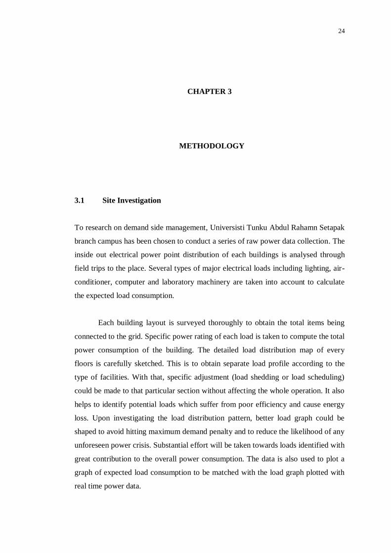
In order to collect real time power data series, a power analyser which is capable of

tapping real time voltage and current is installed in each existing building within the

campus. The model is TES-3600 3P4W Power Analyser as shown in Figure 3.1. The

display of the power analyser is completed with real power, reactive power and also

neutral current besides showing the fed in three phase voltages and currents. A

functional power analyser has four crocodile clips and four clamps which are for

voltage and current instrumentation respectively. The supported operating modes are

1P2W, 1P3W, 3P3W2M and 3P3W. It also comes with internal memory to store up a

maximum of 10,000 sets of data at any given time interval.

Figure 3.1: TES-3600 3P4W Power Analyser

Before proceeding to switchyards to deploy power analysers, permission

from utility personnel is a must to bring the device along with a laptop to read the

data in graphical form through a user interface designed using NI LabVIEW. All the

four clamps are clamped onto wires directly for current readings while having live

busbars clipped with the crocodile clips to obtain voltage readings. Both sets of

instrumentation must come together so that the device can properly register the

values. The power analyser will be placed inside the switchyard for roughly a week

in order to fill up its maximum capacity. The data is retrieved by connecting the

device to any computer supported with RS232 port and can be saved into any

readable spreadsheet format. It not only consists of current and voltage readings, but

also a comprehensive list of other useful parameters.

26

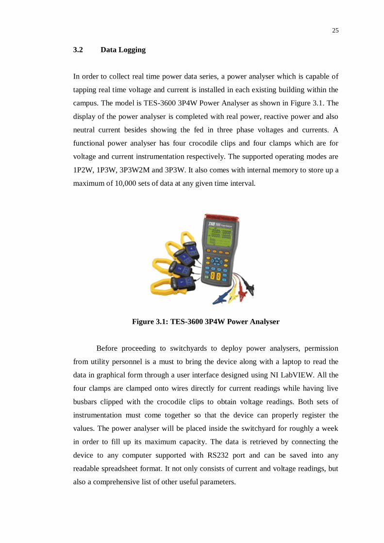
The complete setup of data logging process is shown in Figure 3.2 which

includes a unit of laptop and two units of power analysers. There will be a total of

10080 (60 x 24 x 7) sets of data. Since the collection of data is limited to 10,000 per

unit of power analyser, we have placed in two units of power analysers to record the

extra 80 sets. The two analysers are initiated at two different time so to cover the

extra sets for each other. Power analyser is able to operate without an active

connection to a computer unit. A computer unit is only required upon the collection

of data from the power analyser. The retrieval of data could also be done after the

disconnection of power analyser from the live busbar because the device has its own

internal memory to store the data even it is not powered on. The use of two power

analysers allows us to perform a check on the data if any one set of the data is not

correctly recorded. One of them could always serve as a backup to the other if one of

them fails to operate.

Figure 3.2: Complete Setup of Data Logging Process

27

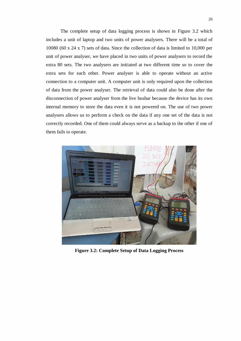
There are four current clamps and four voltage crocodile clips on each unit of

power analyser. The first three pairs of clamp and clip are used to measure three

phase power, namely phase A, phase B and phase C. The reading of neutral current is

taken using the last pair of clamp and clip. In order to measure power, both clamp

and clip must be installed together. Each of them is put onto live busbars with

extreme care to prevent short circuit within the busbars as shown in Figure 3.3.

Wearing insulating rubber gloves is a must under normal proceedings.

Figure 3.3: Clamping Onto Live Busbars

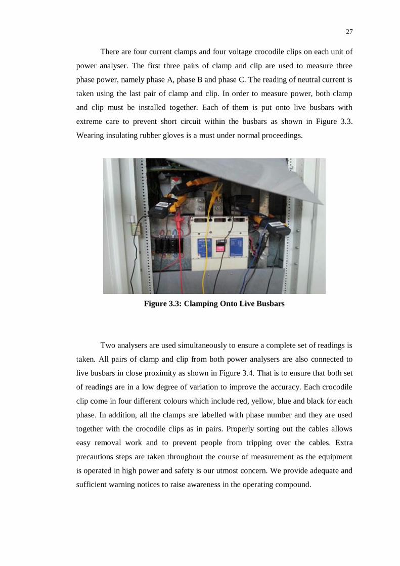
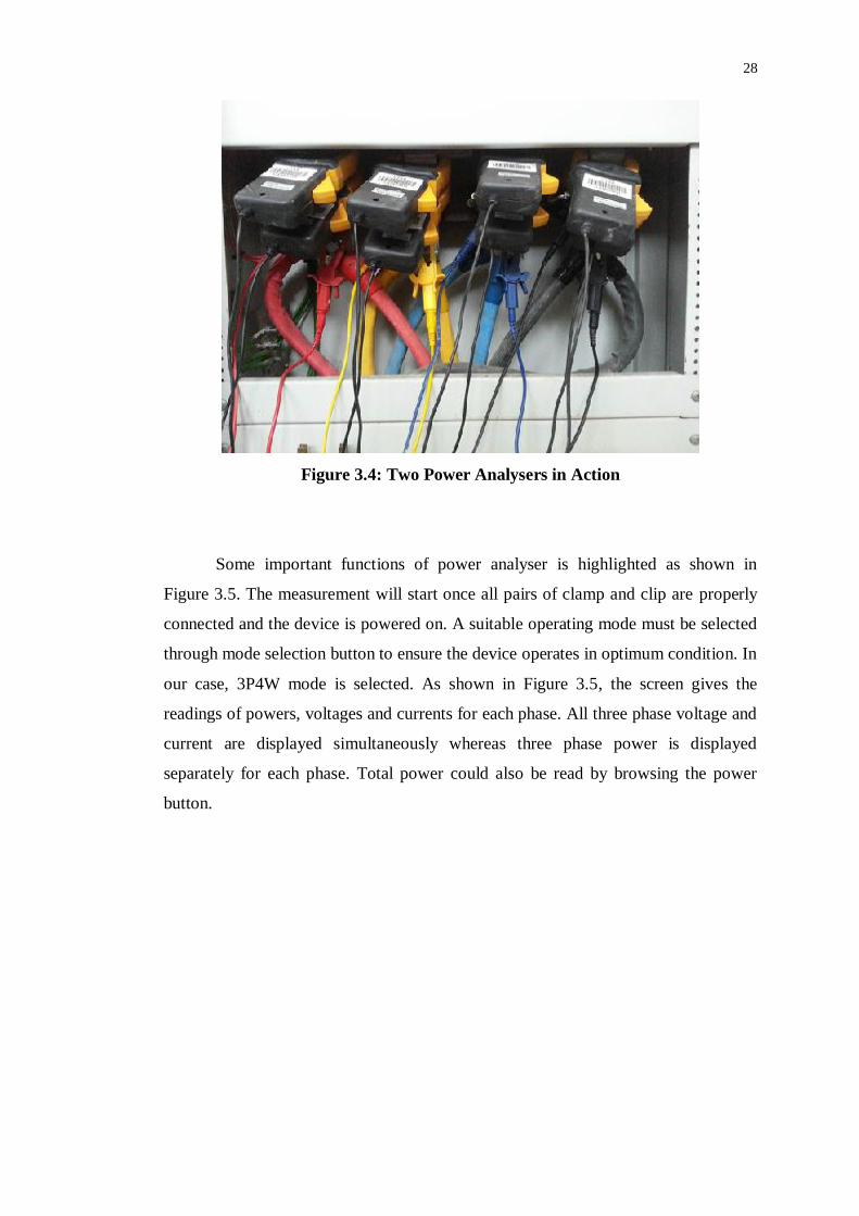
Two analysers are used simultaneously to ensure a complete set of readings is

taken. All pairs of clamp and clip from both power analysers are also connected to

live busbars in close proximity as shown in Figure 3.4. That is to ensure that both set

of readings are in a low degree of variation to improve the accuracy. Each crocodile

clip come in four different colours which include red, yellow, blue and black for each

phase. In addition, all the clamps are labelled with phase number and they are used

together with the crocodile clips as in pairs. Properly sorting out the cables allows

easy removal work and to prevent people from tripping over the cables. Extra

precautions steps are taken throughout the course of measurement as the equipment

is operated in high power and safety is our utmost concern. We provide adequate and

sufficient warning notices to raise awareness in the operating compound.

28

Figure 3.4: Two Power Analysers in Action

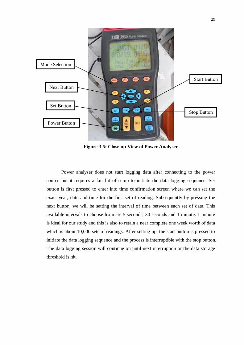
Some important functions of power analyser is highlighted as shown in

Figure 3.5. The measurement will start once all pairs of clamp and clip are properly

connected and the device is powered on. A suitable operating mode must be selected

through mode selection button to ensure the device operates in optimum condition. In

our case, 3P4W mode is selected. As shown in Figure 3.5, the screen gives the

readings of powers, voltages and currents for each phase. All three phase voltage and

current are displayed simultaneously whereas three phase power is displayed

separately for each phase. Total power could also be read by browsing the power

button.

29

Figure 3.5: Close up View of Power Analyser

Power analyser does not start logging data after connecting to the power

source but it requires a fair bit of setup to initiate the data logging sequence. Set

button is first pressed to enter into time confirmation screen where we can set the

exact year, date and time for the first set of reading. Subsequently by pressing the

next button, we will be setting the interval of time between each set of data. This

available intervals to choose from are 5 seconds, 30 seconds and 1 minute. 1 minute

is ideal for our study and this is also to retain a near complete one week worth of data

which is about 10,000 sets of readings. After setting up, the start button is pressed to

initiate the data logging sequence and the process is interruptible with the stop button.

The data logging session will continue on until next interruption or the data storage

threshold is hit.

Set Button

Start Button

Stop Button

Next Button

Mode Selection

Power Button

30

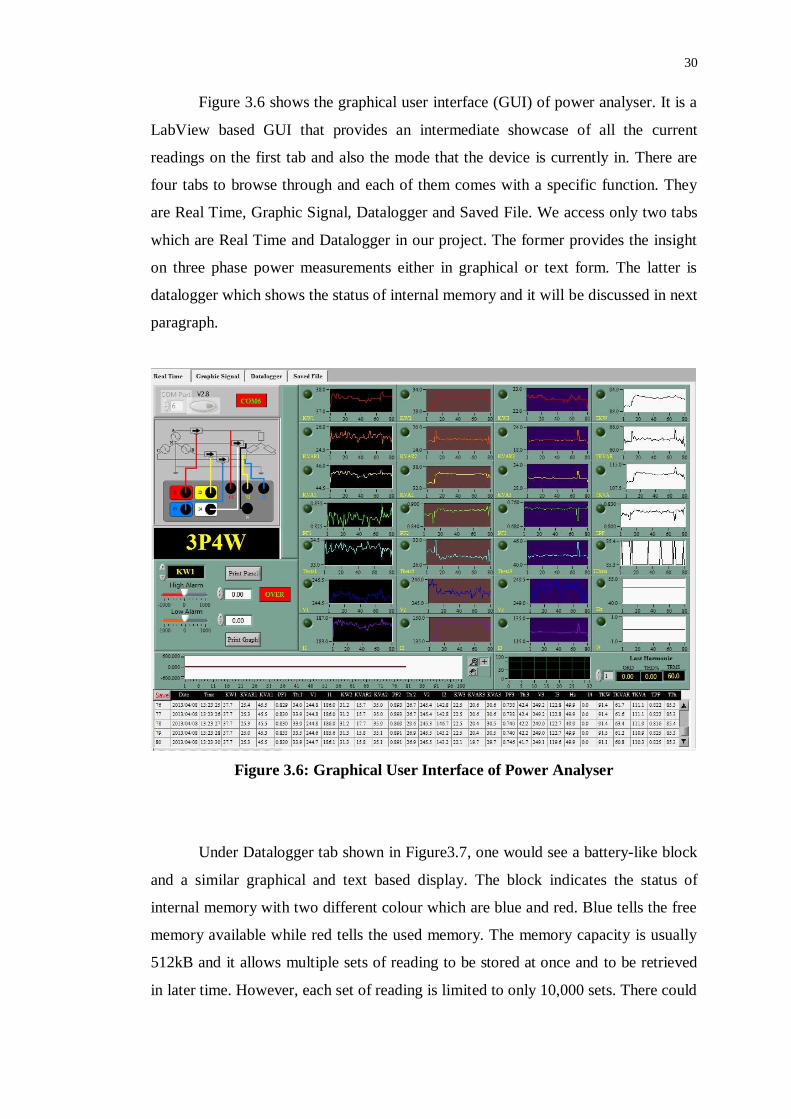
Figure 3.6 shows the graphical user interface (GUI) of power analyser. It is a

LabView based GUI that provides an intermediate showcase of all the current

readings on the first tab and also the mode that the device is currently in. There are

four tabs to browse through and each of them comes with a specific function. They

are Real Time, Graphic Signal, Datalogger and Saved File. We access only two tabs

which are Real Time and Datalogger in our project. The former provides the insight

on three phase power measurements either in graphical or text form. The latter is

datalogger which shows the status of internal memory and it will be discussed in next

paragraph.

Figure 3.6: Graphical User Interface of Power Analyser

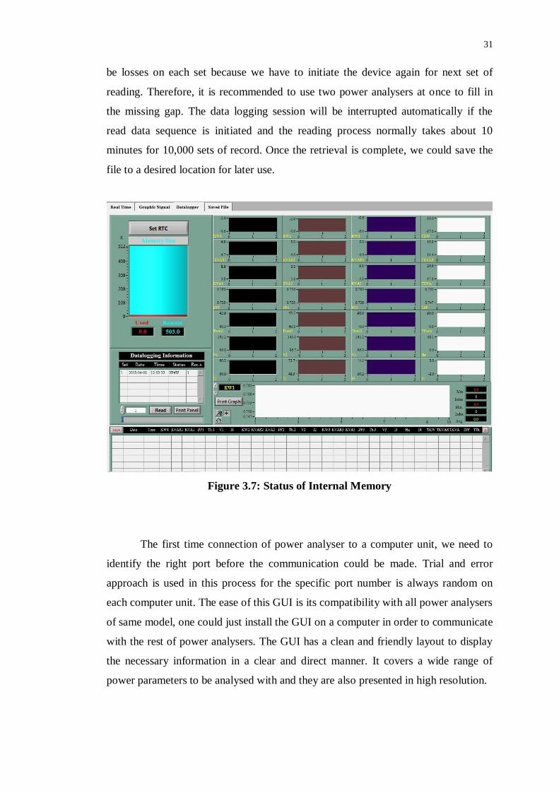
Under Datalogger tab shown in Figure3.7, one would see a battery-like block

and a similar graphical and text based display. The block indicates the status of

internal memory with two different colour which are blue and red. Blue tells the free

memory available while red tells the used memory. The memory capacity is usually

512kB and it allows multiple sets of reading to be stored at once and to be retrieved

in later time. However, each set of reading is limited to only 10,000 sets. There could

31

be losses on each set because we have to initiate the device again for next set of

reading. Therefore, it is recommended to use two power analysers at once to fill in

the missing gap. The data logging session will be interrupted automatically if the

read data sequence is initiated and the reading process normally takes about 10

minutes for 10,000 sets of record. Once the retrieval is complete, we could save the

file to a desired location for later use.

Figure 3.7: Status of Internal Memory

The first time connection of power analyser to a computer unit, we need to

identify the right port before the communication could be made. Trial and error

approach is used in this process for the specific port number is always random on

each computer unit. The ease of this GUI is its compatibility with all power analysers

of same model, one could just install the GUI on a computer in order to communicate

with the rest of power analysers. The GUI has a clean and friendly layout to display

the necessary information in a clear and direct manner. It covers a wide range of

power parameters to be analysed with and they are also presented in high resolution.

32

As a conclusion, the operating mode must be 3P4W for the supply side

provides three phase power. The date and time stored in power analysers are

corrected to keep an accurate data logging period. Meanwhile, the time interval is set

to read the values every one minute until it reaches 10,000 sets of records. All the

readings of each parameter will then be converted to graphical form in excel

spreadsheet to study their trends.

3.3 Graph Tools

All the data are eventually loaded into a spreadsheet program which is Micros to be

processed. The expected outcome would be analysis in tabular or graphical form.

Several approaches are introduced to deal with such large amount of data. All data

are loaded in spreadsheet format where they are divided and arranged by rows and

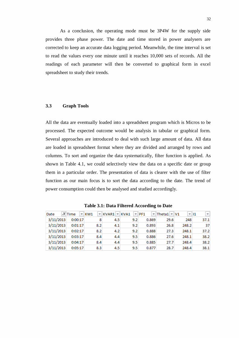
columns. To sort and organize the data systematically, filter function is applied. As

shown in Table 4.1, we could selectively view the data on a specific date or group

them in a particular order. The presentation of data is clearer with the use of filter

function as our main focus is to sort the data according to the date. The trend of

power consumption could then be analysed and studied accordingly.

Table 3.1: Data Filtered According to Date

33

However, there are 1440 sets of data point recorded for each day for the time

interval set between data is 1 minute. To further reduce the data points, we consider

to find the average of every 15 sets of data points. The resultant amount of data point

would be 96 sets which is greatly reduced down from the original 1440 sets. The

reduction is to find relevance of data points to the analysis later. The average of

every 15 sets or 30 sets could then be used to study the occurrence peak demand

which is the highest amount of electricity used within any consecutive period of

thirty minutes.

The average of every 15 sets of data points is calculated with the use of the

spreadsheet program’s built in formula function. The precise calculation of the

average is performed on the 1440 sets of data points for each day. The resultant 96

sets of data points are calculated with ease with the formula shown below. The

formula is built upon the basic math function of average which is provided within the

spreadsheet program. It is modified to start reading the column, C2 to the end and

display the result in the column, D2. The specific interval of the average is stated at

the end.

=AVERAGE(OFFSET(C$2,(ROW()-ROW(D$2))*15,,15,)) (3.1)

Correlation coefficient is used to tell the linear relationship between two sets

of variable whether they could be put together for comparison. The correlation

coefficient is automatically calculated by selecting the data by columns or by rows.

Meanwhile, histogram is used to find out the occurrence frequency for a given range

of value. The range of value is categorized into several groups with an increment of

5kW, starting from 0 to 140kW. The frequency of each group is displayed in both

tabular and graphical forms. Both of these analytical function could be accessed from

Data Analysis packs provided within the spreadsheet program.

34

CHAPTER 4

4 RESULTS AND DISCUSSION

4.1 Introduction

A month of raw power data is logged using the power analyser. The load profile

analysis is performed solely on the total power consumption. They are processed in

Microsoft Excel to obtain an average reading of every 15 minute for each weekday.

Correlation coefficients on each weekday are tabulated along with a combined graph

to show the strong relation between weekdays.

Furthermore, the processed data are presented in histogram to identify the

frequencies of peak power consumption on each successive day. The result consists

only the occurrence of peak power on weekdays because the total power

consumption on weekend falls below the average. Maximum demand surcharges

could be avoided by supplying the calculated required energy. Besides, a regulation

on the power consumption of air conditioning could also save on electricity bills.

4.2 Total Power Consumption

Total power consumption (TKWh) is of importance in the load profile analysis

because the occurrence of maximum power is observed from the total power

consumption. It is the sum of average powers from all three phases. A total of 1440

sets of data were taken through power analyser at the time interval of 1 minute.

35

In order to scale down the data size, the data recorded at the interval of 1

minute are further reduced by taking the average of every 15 sets of the overall data.

There are a total of 96 sets of data are used for the load profile analysis on each day.

Four sets of data are collected for each weekday and their average are taken to do the

comparison on their power consumption trends.

4.3 Weekdays Analysis

4.3.1 Correlation Coefficient and Graph

Table 4.1 shows the correlation coefficient between any two days of weekdays. It is

defined as the measure of the strength of the straight-line or linear dependency of

two variables or sets of data. The correlation coefficient takes on a number between 1

and -1 calculated. A strong positive linear relationship is expected when the values

fall between 0.7 and 1.0.

4.3.1.1 Correlation Coefficient of Mondays

Table 4.1 shows the correlation coefficient of four Mondays. Each pair of them has

strong positive linear relationship with correlation coefficients all above 0.7 as

calculated using the spreadsheet program, ranges from 0.9539 to 0.9842. This allows

us to combine all four sets into a set by finding their average.

Table 4.1: Correlation Coefficients of Mondays

Monday March 11 March 18 March 25 April 1

March 11 1.0000

March 18 0.9765 1.0000

March 25 0.9539 0.9824 1.0000

April 1 0.9661 0.9807 0.9715 1.0000

36

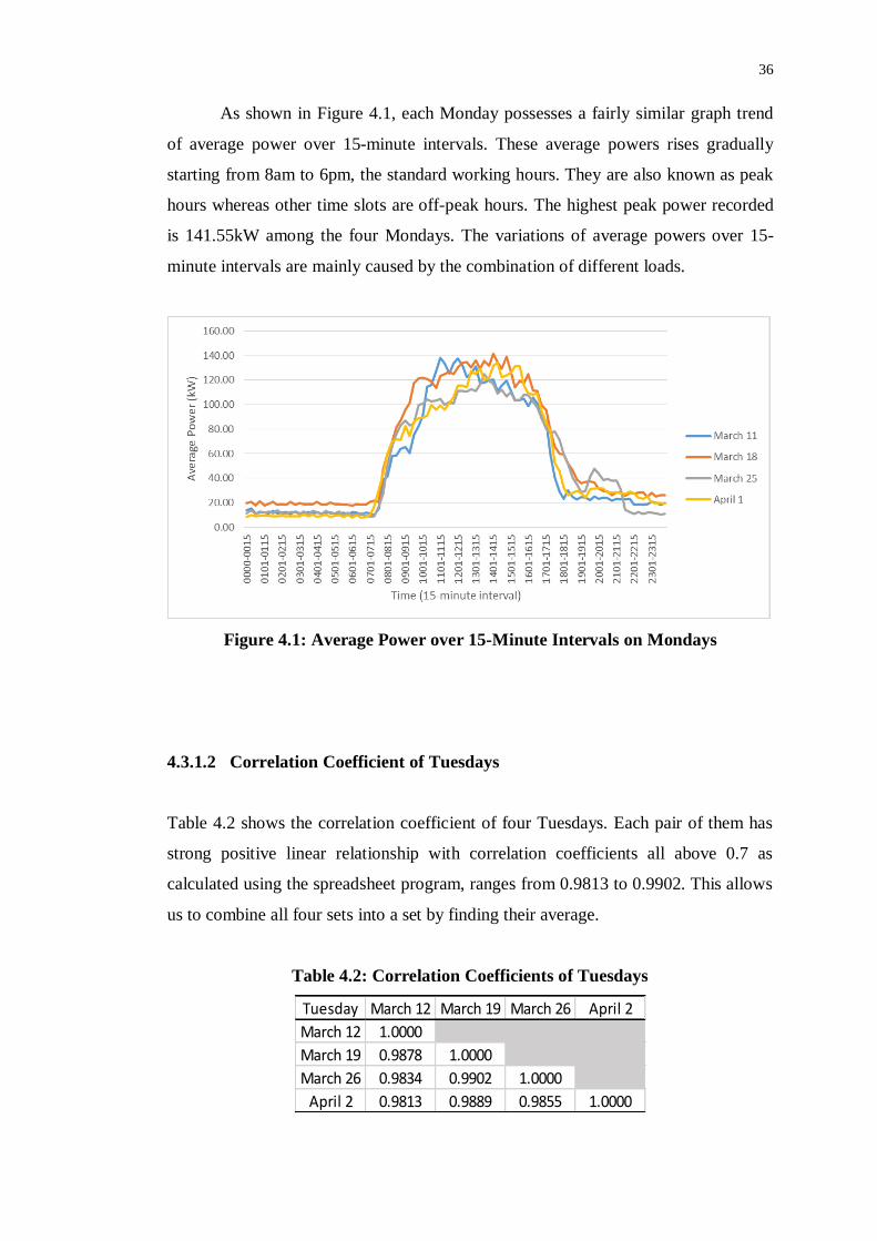
As shown in Figure 4.1, each Monday possesses a fairly similar graph trend

of average power over 15-minute intervals. These average powers rises gradually

starting from 8am to 6pm, the standard working hours. They are also known as peak

hours whereas other time slots are off-peak hours. The highest peak power recorded

is 141.55kW among the four Mondays. The variations of average powers over 15-

minute intervals are mainly caused by the combination of different loads.

Figure 4.1: Average Power over 15-Minute Intervals on Mondays

4.3.1.2 Correlation Coefficient of Tuesdays

Table 4.2 shows the correlation coefficient of four Tuesdays. Each pair of them has

strong positive linear relationship with correlation coefficients all above 0.7 as

calculated using the spreadsheet program, ranges from 0.9813 to 0.9902. This allows

us to combine all four sets into a set by finding their average.

Table 4.2: Correlation Coefficients of Tuesdays

Tuesday March 12 March 19 March 26 April 2

March 12 1.0000

March 19 0.9878 1.0000

March 26 0.9834 0.9902 1.0000

April 2 0.9813 0.9889 0.9855 1.0000

37

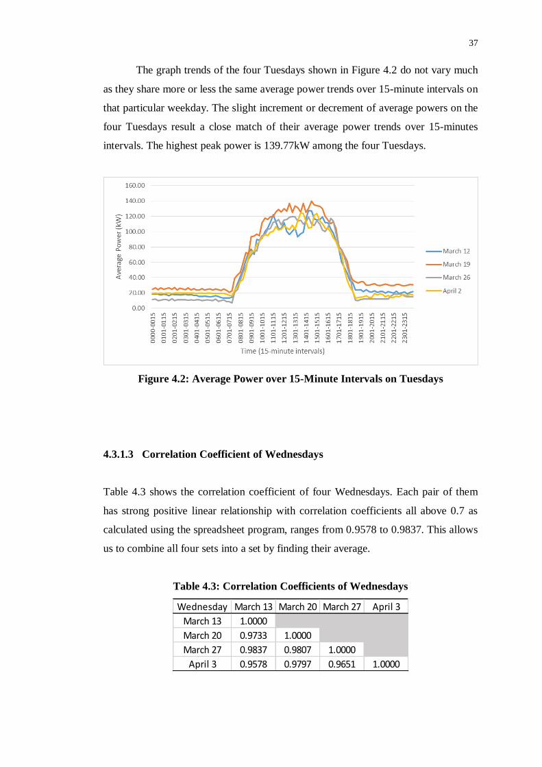
The graph trends of the four Tuesdays shown in Figure 4.2 do not vary much

as they share more or less the same average power trends over 15-minute intervals on

that particular weekday. The slight increment or decrement of average powers on the

four Tuesdays result a close match of their average power trends over 15-minutes

intervals. The highest peak power is 139.77kW among the four Tuesdays.

Figure 4.2: Average Power over 15-Minute Intervals on Tuesdays

4.3.1.3 Correlation Coefficient of Wednesdays

Table 4.3 shows the correlation coefficient of four Wednesdays. Each pair of them

has strong positive linear relationship with correlation coefficients all above 0.7 as

calculated using the spreadsheet program, ranges from 0.9578 to 0.9837. This allows

us to combine all four sets into a set by finding their average.

Table 4.3: Correlation Coefficients of Wednesdays

Wednesday March 13 March 20 March 27 April 3

March 13 1.0000

March 20 0.9733 1.0000

March 27 0.9837 0.9807 1.0000

April 3 0.9578 0.9797 0.9651 1.0000

38

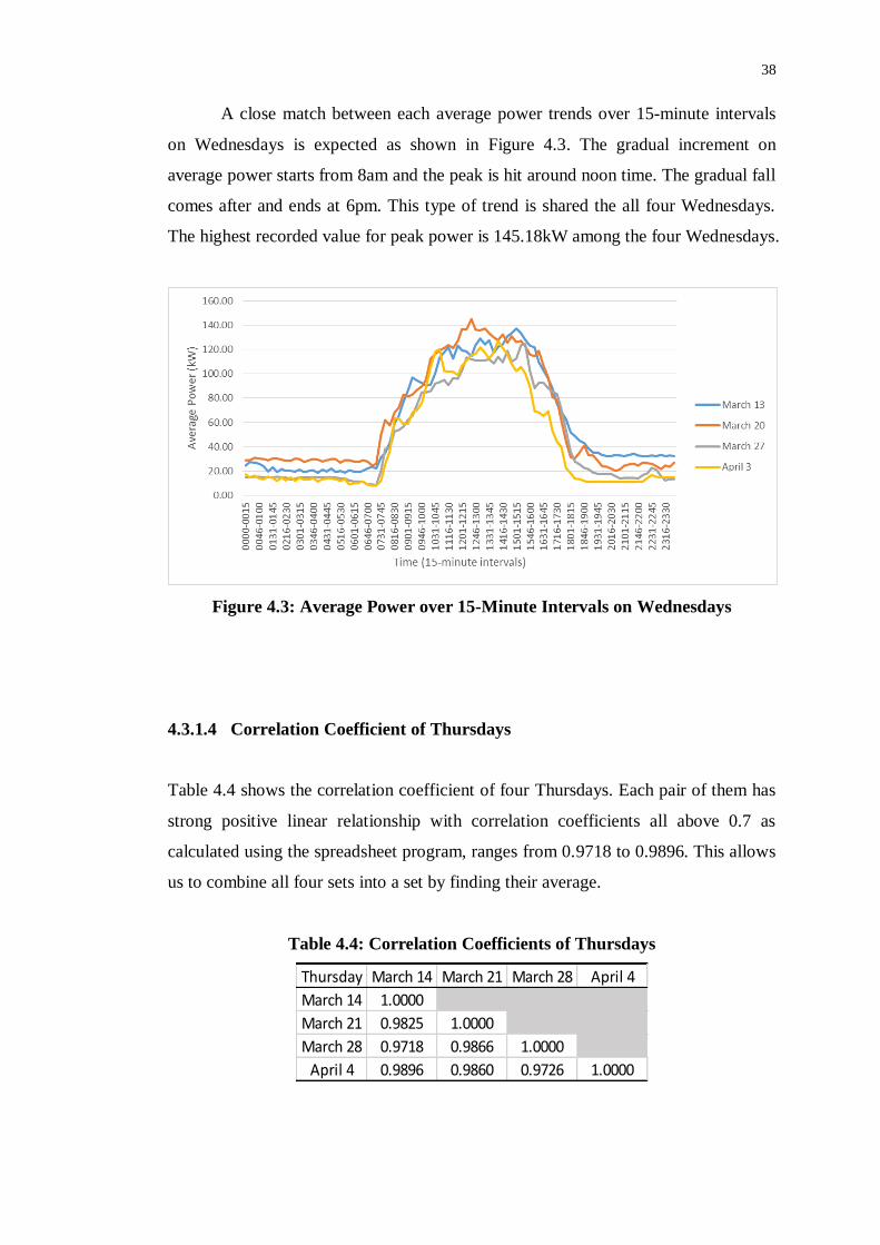
A close match between each average power trends over 15-minute intervals

on Wednesdays is expected as shown in Figure 4.3. The gradual increment on

average power starts from 8am and the peak is hit around noon time. The gradual fall

comes after and ends at 6pm. This type of trend is shared the all four Wednesdays.

The highest recorded value for peak power is 145.18kW among the four Wednesdays.

Figure 4.3: Average Power over 15-Minute Intervals on Wednesdays

4.3.1.4 Correlation Coefficient of Thursdays

Table 4.4 shows the correlation coefficient of four Thursdays. Each pair of them has

strong positive linear relationship with correlation coefficients all above 0.7 as

calculated using the spreadsheet program, ranges from 0.9718 to 0.9896. This allows

us to combine all four sets into a set by finding their average.

Table 4.4: Correlation Coefficients of Thursdays

Thursday March 14 March 21 March 28 April 4

March 14 1.0000

March 21 0.9825 1.0000

March 28 0.9718 0.9866 1.0000

April 4 0.9896 0.9860 0.9726 1.0000

39

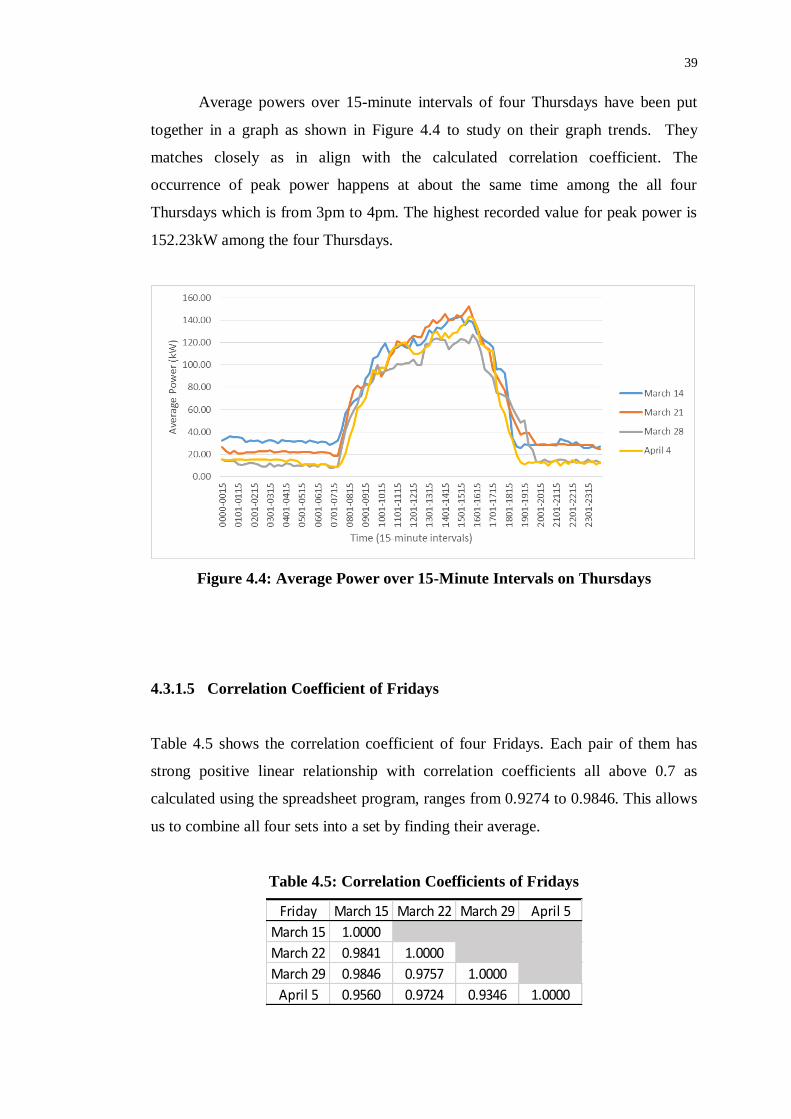
Average powers over 15-minute intervals of four Thursdays have been put

together in a graph as shown in Figure 4.4 to study on their graph trends. They

matches closely as in align with the calculated correlation coefficient. The

occurrence of peak power happens at about the same time among the all four

Thursdays which is from 3pm to 4pm. The highest recorded value for peak power is

152.23kW among the four Thursdays.

Figure 4.4: Average Power over 15-Minute Intervals on Thursdays

4.3.1.5 Correlation Coefficient of Fridays

Table 4.5 shows the correlation coefficient of four Fridays. Each pair of them has

strong positive linear relationship with correlation coefficients all above 0.7 as

calculated using the spreadsheet program, ranges from 0.9274 to 0.9846. This allows

us to combine all four sets into a set by finding their average.

Table 4.5: Correlation Coefficients of Fridays

Friday March 15 March 22 March 29 April 5

March 15 1.0000

March 22 0.9841 1.0000

March 29 0.9846 0.9757 1.0000

April 5 0.9560 0.9724 0.9346 1.0000

40

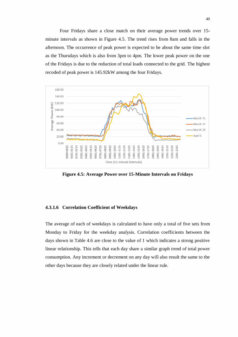
Four Fridays share a close match on their average power trends over 15-

minute intervals as shown in Figure 4.5. The trend rises from 8am and falls in the

afternoon. The occurrence of peak power is expected to be about the same time slot

as the Thursdays which is also from 3pm to 4pm. The lower peak power on the one

of the Fridays is due to the reduction of total loads connected to the grid. The highest

recoded of peak power is 145.92kW among the four Fridays.

Figure 4.5: Average Power over 15-Minute Intervals on Fridays

4.3.1.6 Correlation Coefficient of Weekdays

The average of each of weekdays is calculated to have only a total of five sets from

Monday to Friday for the weekday analysis. Correlation coefficients between the

days shown in Table 4.6 are close to the value of 1 which indicates a strong positive

linear relationship. This tells that each day share a similar graph trend of total power

consumption. Any increment or decrement on any day will also result the same to the

other days because they are closely related under the linear rule.

41

Table 4.6: Correlation Coefficient of Weekdays

Day Monday Tuesday Wednesday Thursday Friday

Monday 1.0000

Tuesday 0.9903 1.0000

Wednesday 0.9881 0.9951 1.0000

Thursday 0.9808 0.9870 0.9901 1.0000

Friday 0.9760 0.9840 0.9778 0.9580 1.0000

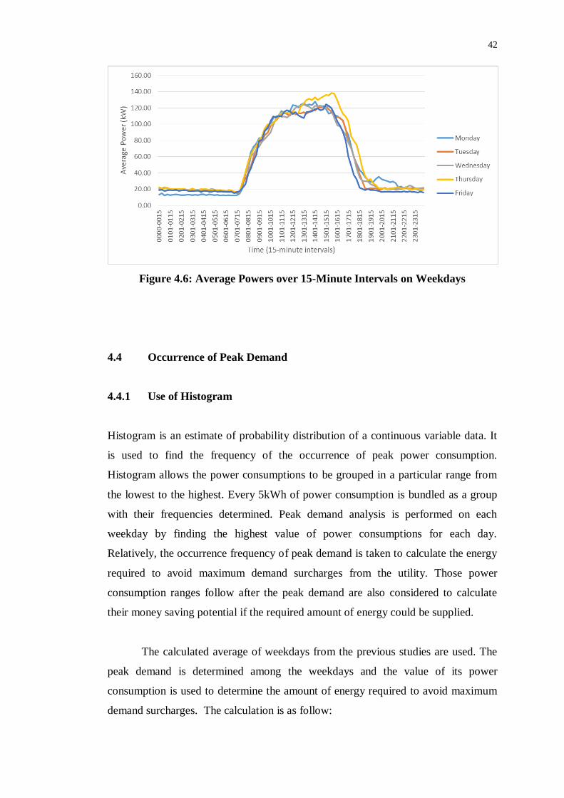
The combined graph shown in Figure 4.6 shows a fairly similar trend of

average power over 15-minute intervals on weekdays. The uprising trend starts at

about 8 in the morning and ends at around 6 in the evening. That period of time is the

standard operating hours for a campus based commercial buildings. Similar

adaptation applies throughout the week. The average power increases gradually over

time and saturates after the noon time. The saturation contributes to the peak demand

whereby the highest peak recorded is on Thursday at 138.59kW around 1530. The

peak demands on other days mostly fall around 120kW or more.

The average power trends over 15-minute intervals on weekdays are very

much affected by the timetable of each day. A day packed with both lab sessions and

tutorial classes will result in higher average powers and also high peak demands due

to the operation of machineries and air-conditioner over long hours. This effect is

prominent on Thursday because it has the highest peak demand across the week.

This analysis could lead to a predictable point of occurrence of peak demand if

enough data points are collected and studied over a several weeks under normal

circumstances.

42

Figure 4.6: Average Powers over 15-Minute Intervals on Weekdays

4.4 Occurrence of Peak Demand

4.4.1 Use of Histogram

Histogram is an estimate of probability distribution of a continuous variable data. It

is used to find the frequency of the occurrence of peak power consumption.

Histogram allows the power consumptions to be grouped in a particular range from

the lowest to the highest. Every 5kWh of power consumption is bundled as a group

with their frequencies determined. Peak demand analysis is performed on each

weekday by finding the highest value of power consumptions for each day.

Relatively, the occurrence frequency of peak demand is taken to calculate the energy

required to avoid maximum demand surcharges from the utility. Those power

consumption ranges follow after the peak demand are also considered to calculate

their money saving potential if the required amount of energy could be supplied.

The calculated average of weekdays from the previous studies are used. The

peak demand is determined among the weekdays and the value of its power

consumption is used to determine the amount of energy required to avoid maximum

demand surcharges. The calculation is as follow:

43

Energy Required = Occurrence Frequency x 5kWh (4.1)

Potential Saving = Energy Required x RM25.90/kWh (4.2)

4.4.1.1 Histograms of Weekdays

Power consumption of weekdays are categorised with their occurrence frequencies

specified. These power consumption groups are set in the range of 0kWh to 140kWh

with a step of 5kWh for each group.

Histograms shown in Figure 4.7, Figure 4.8, Figure 4.9, Figure 4.10 and

Figure 4.11 show the occurrence frequency of each power consumption group from

Monday to Friday. This is to provide the ease of comparing the highest power

consumptions among the weekdays. The relative occurrence frequency is used to

calculate the energy required to save from maximum demand surcharges.

Figure 4.7: Histogram of Monday

44

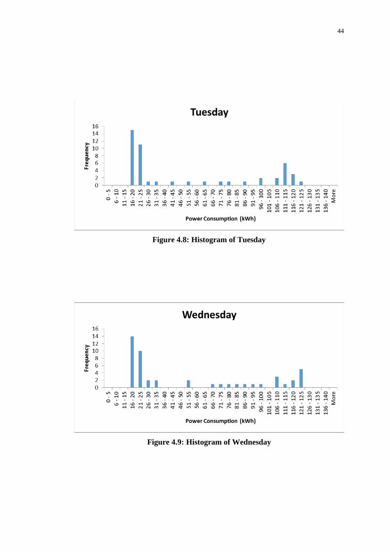
Figure 4.8: Histogram of Tuesday

Figure 4.9: Histogram of Wednesday

45

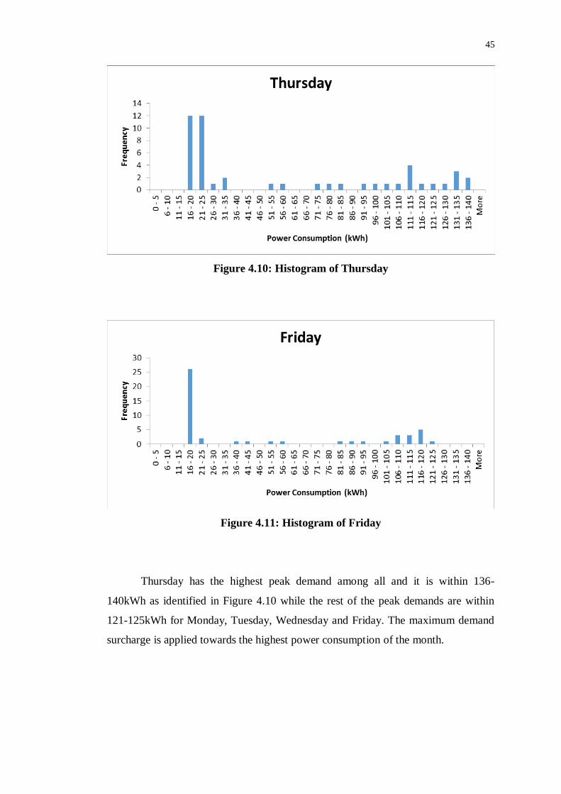
Figure 4.10: Histogram of Thursday

Figure 4.11: Histogram of Friday

Thursday has the highest peak demand among all and it is within 136-

140kWh as identified in Figure 4.10 while the rest of the peak demands are within

121-125kWh for Monday, Tuesday, Wednesday and Friday. The maximum demand

surcharge is applied towards the highest power consumption of the month.

46

In order to avoid that maximum demand surcharge, peak demand on

Thursday could be brought down from 136-140kWh to 131-135kWh. Whenever the

power consumption of that day falls between 136-140kWh, 5kWh of energy will be

supplied to bring down the power consumption from 136-140kWh to 131-135kWh.

The occurrence frequency of peak demand on Thursday is 2 where energy is supplied

for that two occurrences of peak demand.

Energy Required = 2 x 5kWh = 10kWh

Potential Saving = 10kWh x RM25.90/kWh = RM259.00

The amount of energy required to avoid peak demand is 10kWh. By bringing

down the power consumption from 136-140kWh to 131-135kWh, we can avoid the

maximum demand surcharge and achieve a potential saving of RM259.00.

4.4.1.2 Combined Histogram of Weekdays

The histogram in Figure 4.12 shows a combined occurrence frequency of each power

consumption range on weekdays. Each day shares a relatively high frequency of

power consumption from 11kWh to 20kWh. These power consumptions occur

mainly during the off-peak period and they appear to be uniform across weekdays.

The power consumption within 136-140kW is considered to be the peak demand.

From the combined histograms, Thursday has proven to have the highest peak

demand as compared to the other days.

47

Figure 4.12: Occurrence Frequency of Power Consumption on Weekdays

With the use of histogram, power consumption is divided into groups. The

supply of energy is performed whenever the power consumption falls into the group

which constitutes the occurrence of peak demand. Energy is supplied whenever the

power consumption falls within the group which is labelled as the occurrence of peak

demand. On the other hand, by knowing the exact value of peak demand, the energy

is only supplied whenever the peak demand is hit to avoid maximum demand

surcharge for that instance.

4.5 Load Distribution of Tutorial Rooms in SE Block

Another effective way to study the power consumption of a building over a specific

period of time is to breakdown the power consumption onto specific load types. Each

type of load will have different load profile which will result in a different amount of

power consumption. In every session, there will be several types of load being put

together to bring upon the optimum operation.

48

4.5.1 Types of Load

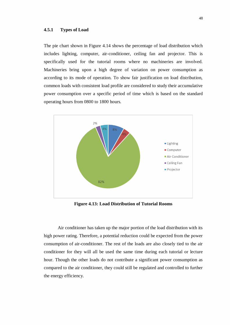
The pie chart shown in Figure 4.14 shows the percentage of load distribution which

includes lighting, computer, air-conditioner, ceiling fan and projector. This is

specifically used for the tutorial rooms where no machineries are involved.

Machineries bring upon a high degree of variation on power consumption as

according to its mode of operation. To show fair justification on load distribution,

common loads with consistent load profile are considered to study their accumulative

power consumption over a specific period of time which is based on the standard

operating hours from 0800 to 1800 hours.

Figure 4.13: Load Distribution of Tutorial Rooms

Air conditioner has taken up the major portion of the load distribution with its

high power rating. Therefore, a potential reduction could be expected from the power

consumption of air-conditioner. The rest of the loads are also closely tied to the air

conditioner for they will all be used the same time during each tutorial or lecture

hour. Though the other loads do not contribute a significant power consumption as

compared to the air conditioner, they could still be regulated and controlled to further

the energy efficiency.

49

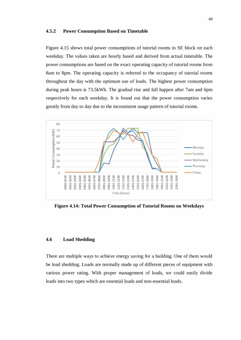
4.5.2 Power Consumption Based on Timetable

Figure 4.15 shows total power consumptions of tutorial rooms in SE block on each

weekday. The values taken are hourly based and derived from actual timetable. The

power consumptions are based on the exact operating capacity of tutorial rooms from

8am to 8pm. The operating capacity is referred to the occupancy of tutorial rooms

throughout the day with the optimum use of loads. The highest power consumption

during peak hours is 73.5kWh. The gradual rise and fall happen after 7am and 6pm

respectively for each weekday. It is found out that the power consumption varies

greatly from day to day due to the inconsistent usage pattern of tutorial rooms.

Figure 4.14: Total Power Consumption of Tutorial Rooms on Weekdays

4.6 Load Shedding

There are multiple ways to achieve energy saving for a building. One of them would

be load shedding. Loads are normally made up of different pieces of equipment with

various power rating. With proper management of loads, we could easily divide

loads into two types which are essential loads and non-essential loads.

50

4.6.1 Essential and Non-essential Loads

Essential loads require active power source to maintain its optimum operation and

they are normally non-interruptible. Non-essential loads are turned on when there is a

demand over a particular period of time. So, essential loads will always be prioritized

over non-essential loads under normal circumstances.

Load shedding scheme has put emphasis on shedding non-essential loads. For

an instance, air-conditioners and lighting in tutorial rooms should be turned off

whenever the rooms are not in use. Non-essential loads can provide immediate relief

towards reduction in power consumption for their characteristics. Essential loads

would also be arranged in such that no two essential loads operate at their maximum

capacities the same time because there is high chance to hit above the maximum

demand threshold. The solution would be to shift the loads to off-peak periods or to

alternate the essential loads to take turn running in their full capacities.

Turning on and off loads based on the requirements would greatly reduce the

power consumption because predictable pattern could be observed to always have the

optimum power consumption. With certain degree of prediction, the loads could be

efficiently scheduled or shed to avoid peak power consumption especially during

peak hours. The unnecessary surcharges could be only avoided if we could have seen

it coming. Nevertheless, loads should be monitored and regulated to operate at their

optimum conditions to achieve better energy efficiency.

4.6.2 Alternate Mean to Reduce Peak Demand

Air conditioner is one of the major power consuming units in overall. This is due to

its high power rating and a large number of units to be installed within a building.

The main purpose is to keep a closed space cool under a certain a low temperature.

Lower temperature setting would require an active exchange of air to bring down the

room temperature and maintain the low temperature. This has in fact made up a

higher power consumption over time.

51

Load shedding could be performed on air conditioner by reducing its power

consumption accordingly. The necessity to power on all units of air conditioner could

be avoided through proper load management. Whenever a class ends, air conditioner

should be switched off to converse the energy. In a small class setting, turning on one

air conditioner would be sufficient instead of more to achieve in reduction of overall

power consumption. In practical, the real power consumption according to the

timetable varies from 45kWh to 50kWh from Monday to Friday. The difference of

the variation provides the possible amount of money could be saved from the

maximum demand surcharges through a reduction in total power consumption of air

conditioner. The reduction could help reduce the peak power and avoid hitting the

maximum demand threshold.

As the power consumption of air conditioner varies from 45kWh to 50kWh,

the maximum possible energy reduction is 5kWh. The energy reduction could be

performed in the step of 1kWh until it reaches the maximum. The reduction will

directly help lower the peak demand of any day. For an instance, an energy reduction

of 5kWh can reduce the peak demand of 136.93kWh on Thursday to 131.93kWh.

Thus, the amount of maximum demand surcharge to be avoided is RM RM3546.49.

4.7 Maximum Demand Surcharge

The occurrence of peak demand within any consecutive period of thirty minutes in a

month will incur a surcharge of maximum demand. By all means, the surcharge is to

be avoided in order to save on the electricity bill. Maximum demand is measured in

kilowatts, and it is calculated as double the highest amount of electricity used (kWh)

within any consecutive period of thirty minutes in a month (Tenaga Nasional Berhad,

n.d.).

52

As identified in the combined graph of weekdays, Thursday shares the most

occurrence of peak demand and also the highest peak demand in value. The

surcharge of maximum demand could be avoided through the clipping of peak

demand. To be specific, the power consumption is maintained below the specific

maximum demand threshold. The additional power demand is supplied by a separate

power grid either from a distributed generator (DG) or a micro-grid. The system to

perform all those is regarded as energy storage system (ESS). It does not only help

prevent maximum surcharge, but also as a backup supply during power outages. It

gives an output of energy to prevent the occurrence of peak demand.

On the other term, the amount of electricity to be penalised would in fact be

the highest power consumption within a specific period. For an example, the amount

of energy required to lower the peak demand would be dependent on the size of ESS.

The surcharge of maximum demand is calculated as RM25.90 per kilowatts-hour of

electricity. Thus, 10kWh of energy is supplied to avoid the maximum demand of

136.93kWh on Thursday. The potential saving will be RM259.00. It would be a large

amount to pay if the occurrence of peak demand is taken on every building. By

injecting power to the grid during peak hours with energy storage system would save

much on the electricity cost in long term. The accumulative amount of surcharges

could also be diverted through proper load management by shifting the major loads

to operate during off peak hours.

53

CHAPTER 5

5 CONCLUSION AND RECOMMENDATIONS

5.1 Conclusion

The analysis presented is considered to be straightforward after having the data

points reduced to its minimum amount. The analysis started off by looking into the

correlation coefficients between any two days because much studies are taken from

the comparison of any two sets of data. Graphical and tabular forms are largely used

to analyse load profiles of SE block where the main focus is on the average powers

trends over 15-minute intervals of weekdays. Load distribution of tutorial rooms is

investigated based the types of load and their power consumption trends.

The occurrence of peak demand is observed through the trend of power

consumption on weekdays. This could be resulted from the packed timetable on that

day and the loads used are with high power rating. The possible occurrence of peak

demand could be predicted based on the past occurrence of peak demand pattern.

The occurrence frequency of peak demand on each weekday is also determined with

the use of histogram. From the results, possible reduction in peak demand is

performed in a step of 5kWh. The uniform power consumption of 11kWh to 20kWh

has the highest frequency for all weekdays which is during off-peak periods.

The peak demand is later suggested to be reduced with the use of energy

storage system to avoid the surcharge of maximum demand. A weekday analysis is

conducted on each weekday to learn the occurrences of peak demand which would

later be used to determine the highest peak demand. We can save on the maximum

54

demand surcharge if we are able to clip away the peak demand by supplying required

energy to maintain the peak demand below the maximum demand threshold. Possible

reduction in power consumption of air conditioner is also investigated to bring down

the peak demand so to avoid maximum demand surcharges.

5.2 Recommendations

Currently, the data logging is limited to manual collection after each session. The

data logged in the power analyser is also restricted to only 10,000 sets. It requires

consistent labour work to check the condition of power analysers on site and to

collect the data manually through a computer unit which has to be brought around

during each session. The recommendation here is to bring the data logging to next

level whereby everything could be done remotely and automatically without moving

much of the existing device.

A central management system would be useful to constantly monitor and

regulate the data logging process remotely. The measurements on three phase power

could be retrieved in real time and monitored from a distant computer unit. This

removes the requirement of consistent visit to the site to check the condition of

power analyser. Consistent health checking signal can be sent to the device from

time to time. If a problem is identified through remote monitoring, immediate action

could be taken right after. This in fact ensures the continuity of data logging process

and to retrieve data at ease. By implementing advanced control algorithms, the

system could perform self-regulation towards external stimuli. For an instance, the

system would know when to raise an alert to the consumer if the power consumption

has hit a certain limit which would incur surcharges. This smart system is

reconfigurable to suit the needs of consumer towards multiple scenarios. On a higher

level, controls could be exerted from the central management system to solve the

problem without the need to alert consumers. However, the activity of the system

would still be monitored by the consumer to ensure an optimum operation.

55

REFERENCES

REEEP/UNIDO Training Package, n.d. Sustainable Energy Regulation and

Policymaking for Africa: Demand Side Management. [Online]. Available at:

http://africa-toolkit.reeep.org/modules/Module14.pdf [Accessed 30 March 2013].

Cogeneration Technologies, n.d. Demand Side Management. [Online]. Available at:

http://cogeneration.net/demand-side-management [Accessed 30 March 2013].

Venkateswara Sarma Mallela, Parmal Singh Solanki and Yousif Juma Ali Al-Harasi,

2011. Regulation of Energy Demands via DSM Policies: A Case Study in Oman,

[E-journal] 1, 1, 54(6), Available through AM Publishers website

http://www.ampublisher.com/. [Accessed 30 March 2013].

Palensky, P. and Dietrich, D., 2011. Demand Side Management: Demand Response,

Intelligent Energy Systems, and Smart Loads, [E-journal] 7, 3, 381(8), Available

through IEEE Xplore Digital Library website http://ieeexplore.ieee.org/.

[Accessed 31 March 2013].

Boshell, F. and Veloza, O.P., 2008. Review of developed demand side management

programs including different concepts and their results. Transmission and

Distribution Conference and Exposition, Bogota, 20- 13-15 Aug. Available at:

http://ieeexplore.ieee.org.libezp.utar.edu.my/stamp/stamp.jsp?tp=&arnumber=464

1792. [Accessed 31 March 2013].

S. Alyasin, et al., 1994. Selected Topics on Demand Side Management. Purdue

University. Available through Purdue University Library website http://

docs.lib.purdue.edu/cgi/viewcontent.cgi?article=1186&context=ecetr [Accessed

31 March 2013].

Choi, S.S., Tseng, K.J., Vilathgamuwa, D.M. and Nguyen, T.D., 2008. Energy

storage systems in distributed generation schemes. Power and Energy Society

General Meeting - Conversion and Delivery of Electrical Energy in the 21st

Century, Pittsburgh, 20-24 July. Available at:

http://ieeexplore.ieee.org.libezp.utar.edu.my/stamp/stamp.jsp?tp=&arnumber=459

6169/. [Accessed 6 April 2013].

Schainker, Robert B., 2004. Executive overview: energy storage options for a

sustainable energy future. Power Engineering Society General Meeting, Denver,

10 June. Available at: http://ieeexplore.ieee.org.libezp.utar.edu.my/stamp/

stamp.jsp?tp=&arnumber=1373298/. [Accessed 6 April 2013].

56

Singh, Rayman Preet, Gao, Peter Xiang and Lizotte, Daniel J., 2012. On hourly home

peak load prediction. Smart Grid Communications in 2012 IEEE Third

International Conference, Tainan, 5-8 Nov. Available at:

http://ieeexplore.ieee.org.libezp.utar.edu.my/stamp/stamp.jsp?tp=&arnumber=648

5977/. [Accessed 6 April 2013].

Costanzo, G.T., Guchuan Zhu; Anjos, M.F. and Savard, G., 2012. A System

Architecture for Autonomous Demand Side Load Management in Smart Buildings,

[E-journal] 3, 4, 2157(9), Available through IEEE Xplore Digital Library website

http://ieeexplore.ieee.org/. [Accessed 7 April 2013].

Ying Guo, Rongxin Li, Poulton, G. and Zeman, A., 2008. A Simulator for Self-

Adaptive Energy Demand Management. Self-Adaptive and Self-Organizing

Systems in Second IEEE International Conference, Venezia, 20-24 Oct. Available

at: http://ieeexplore.ieee.org.libezp.utar.edu.my/stamp/stamp.jsp?tp=&arnumber=

4663411/. [Accessed 7 April 2013].

Yogesh Simmhan, et al., 2012. Adaptive Energy Forecasting and Information

Diffusion for Smart Power Grids. IEEE International Scalable Computing

Challenge (SCALE), 1(4), Available at: http://ceng.usc.edu/~simmhan/

pubs/simmhan-scale-2012.pdf/. [Accessed 30 March 2013]

Tenaga Nasional Berhad, n.d. Maximum Demand. [Online]. Available at:

http://www.tnb.com.my/business/for-commercial/maximum-demand.html

[Accessed 7 April 2013].