Embed Size (px)
Citation preview
Model Linear equilibrium Demand and supply shocks Monetary Policy Welfare Transparency Wrapping up
Demand Shocks with Dispersed Information
Guido Lorenzoni (MIT)
Class notes, 06 March 2007
Cite as: Guido Lorenzoni, course materials for 14.462 Advanced Macroeconomics II, Spring 2007. MIT OpenCourseWare (http://ocw.mit.edu/), Massachusetts Institute of Technology. Downloaded on [DD Month YYYY].
Model Linear equilibrium Demand and supply shocks Monetary Policy Welfare Transparency Wrapping up
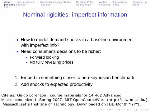
Nominal rigidities: imperfect information
How to model demand shocks in a baseline environment •
with imperfect info?Need consumer’s decisions to be richer:•
• Forward looking • No fully revealing prices
1. Embed in something closer to neo-keynesian benchmark
2. Add shocks to expected productivity
Cite as: Guido Lorenzoni, course materials for 14.462 Advanced Macroeconomics II, Spring 2007. MIT OpenCourseWare (http://ocw.mit.edu/), Massachusetts Institute of Technology. Downloaded on [DD Month YYYY].
Model Linear equilibrium Demand and supply shocks Monetary Policy Welfare Transparency Wrapping up
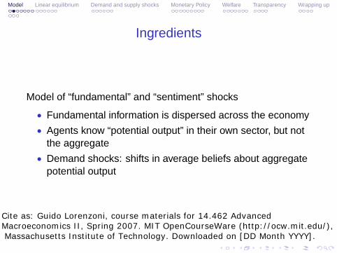
Ingredients
Model of “fundamental” and “sentiment” shocks
• Fundamental information is dispersed across the economy
• Agents know “potential output” in their own sector, but not the aggregate
• Demand shocks: shifts in average beliefs about aggregate potential output
Cite as: Guido Lorenzoni, course materials for 14.462 Advanced Macroeconomics II, Spring 2007. MIT OpenCourseWare (http://ocw.mit.edu/), Massachusetts Institute of Technology. Downloaded on [DD Month YYYY].
� �
Model Linear equilibrium Demand and supply shocks Monetary Policy Welfare Transparency Wrapping up
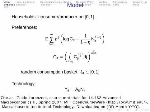
Model
Households: consumer/producer on [0,1].
Preferences:
∞
∑ β t logCit − 1 +
1 η
Nit 1+ηE
t=0 �� � σ σ −1 σ−1
Cit = Jit
Cijt σ dj
random consumption basket: Jit ⊂ [0,1]
Technology: Yit = AitNit
Cite as: Guido Lorenzoni, course materials for 14.462 Advanced Macroeconomics II, Spring 2007. MIT OpenCourseWare (http://ocw.mit.edu/), Massachusetts Institute of Technology. Downloaded on [DD Month YYYY].
Model Linear equilibrium Demand and supply shocks Monetary Policy Welfare Transparency Wrapping up
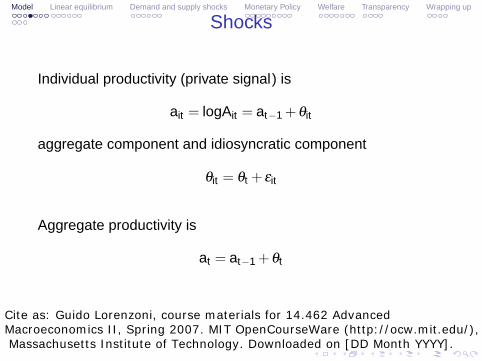
Shocks
Individual productivity (private signal) is
ait = logAit = at−1 + θit
aggregate component and idiosyncratic component
θit = θt + εit
Aggregate productivity is
at = at−1 + θt
Cite as: Guido Lorenzoni, course materials for 14.462 Advanced Macroeconomics II, Spring 2007. MIT OpenCourseWare (http://ocw.mit.edu/), Massachusetts Institute of Technology. Downloaded on [DD Month YYYY].
Wrapping up
Model Linear equilibrium Demand and supply shocks Monetary Policy Welfare Transparency
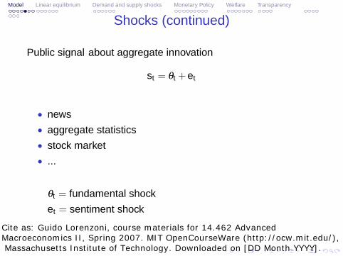
Shocks (continued)
Public signal about aggregate innovation
st = θt + et
• news
• aggregate statistics
stock market•
...•
θt = fundamental shock
et = sentiment shock
Cite as: Guido Lorenzoni, course materials for 14.462 Advanced Macroeconomics II, Spring 2007. MIT OpenCourseWare (http://ocw.mit.edu/), Massachusetts Institute of Technology. Downloaded on [DD Month YYYY].
Model Linear equilibrium Demand and supply shocks Monetary Policy Welfare Transparency Wrapping up
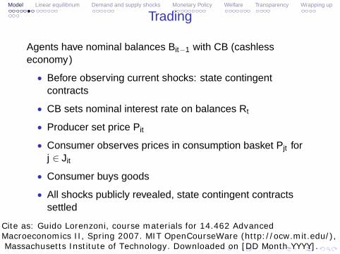
Trading
Agents have nominal balances Bit−1 with CB (cashless economy )
• Before observing current shocks: state contingentcontracts
• CB sets nominal interest rate on balances Rt
• Producer set price Pit
• Consumer observes prices in consumption basket Pjt for j ∈ Jit
• Consumer buys goods
• All shocks publicly revealed, state contingent contracts settled
Cite as: Guido Lorenzoni, course materials for 14.462 Advanced Macroeconomics II, Spring 2007. MIT OpenCourseWare (http://ocw.mit.edu/), Massachusetts Institute of Technology. Downloaded on [DD Month YYYY].

� �
Model Linear equilibrium Demand and supply shocks Monetary Policy Welfare Transparency Wrapping up
Budget constraint
Bit = Rt Bit−1 +(1 + τ)PitYit − PitCit + Zit (ht ) − Tt
− �
qt � ht
� Zit
� ht
� dh̃t . ˜ ˜
• Pit price index for goods in Jit
• Z state contingent contracts
• subsidy τ to correct for monopolistic distortion
• Tt lump sum tax to finance subsidy
Cite as: Guido Lorenzoni, course materials for 14.462 Advanced Macroeconomics II, Spring 2007. MIT OpenCourseWare (http://ocw.mit.edu/), Massachusetts Institute of Technology. Downloaded on [DD Month YYYY].
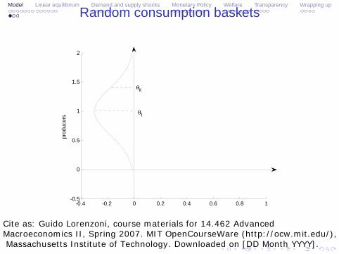
Model Linear equilibrium Demand and supply shocks Monetary Policy Welfare Transparency Wrapping up
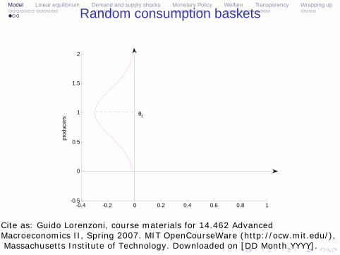
Random consumption baskets
-0.4 -0.2 0 0.2 0.4 0.6 0.8 1-0.5
0
0.5
1
1.5
2
prod
ucer
s θt
Figure 1:
1
Cite as: Guido Lorenzoni, course materials for 14.462 Advanced Macroeconomics II, Spring 2007. MIT OpenCourseWare (http://ocw.mit.edu/), Massachusetts Institute of Technology. Downloaded on [DD Month YYYY].
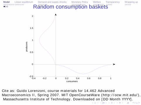
Model Linear equilibrium Demand and supply shocks Monetary Policy Welfare Transparency Wrapping up
Random consumption baskets
-0.4 -0.2 0 0.2 0.4 0.6 0.8 1-0.5
0
0.5
1
1.5
2
prod
ucer
s θt
θit
Figure 2:
2
Cite as: Guido Lorenzoni, course materials for 14.462 Advanced Macroeconomics II, Spring 2007. MIT OpenCourseWare (http://ocw.mit.edu/), Massachusetts Institute of Technology. Downloaded on [DD Month YYYY].
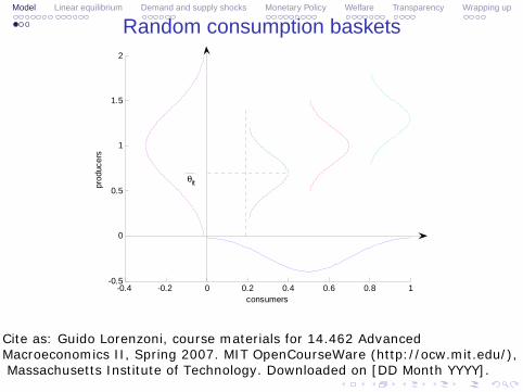
Model Linear equilibrium Demand and supply shocks Monetary Policy Welfare Transparency Wrapping up
Random consumption baskets
-0.4 -0.2 0 0.2 0.4 0.6 0.8 1-0.5
0
0.5
1
1.5
2
consumers
prod
ucer
s
Figure 3:
3
Cite as: Guido Lorenzoni, course materials for 14.462 Advanced Macroeconomics II, Spring 2007. MIT OpenCourseWare (http://ocw.mit.edu/), Massachusetts Institute of Technology. Downloaded on [DD Month YYYY].
Model Linear equilibrium Demand and supply shocks Monetary Policy Welfare Transparency Wrapping up
Random consumption baskets
-0.4 -0.2 0 0.2 0.4 0.6 0.8 1-0.5
0
0.5
1
1.5
2
consumers
prod
ucer
s
θit
Figure 4:
4
Cite as: Guido Lorenzoni, course materials for 14.462 Advanced Macroeconomics II, Spring 2007. MIT OpenCourseWare (http://ocw.mit.edu/), Massachusetts Institute of Technology. Downloaded on [DD Month YYYY].
� �
Model Linear equilibrium Demand and supply shocks Monetary Policy Welfare Transparency Wrapping up
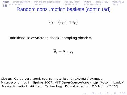
Random consumption baskets (continued)
=θ it θjt : j ∈ Jit
additional idiosyncratic shock: sampling shock vit
θ it = θt + vit
Cite as: Guido Lorenzoni, course materials for 14.462 Advanced Macroeconomics II, Spring 2007. MIT OpenCourseWare (http://ocw.mit.edu/), Massachusetts Institute of Technology. Downloaded on [DD Month YYYY].
� �
Model Linear equilibrium Demand and supply shocks Monetary Policy Welfare Transparency Wrapping up
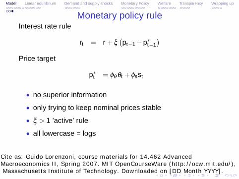
Monetary policy rule Interest rate rule
rt = r + ξ pt−1 − pt ∗−1
Price target
pt ∗ = φθ θt + φsst
• no superior information
• only trying to keep nominal prices stable
ξ > 1 ’active’ rule •
• all lowercase = logs
Cite as: Guido Lorenzoni, course materials for 14.462 Advanced Macroeconomics II, Spring 2007. MIT OpenCourseWare (http://ocw.mit.edu/), Massachusetts Institute of Technology. Downloaded on [DD Month YYYY].
Model Linear equilibrium Demand and supply shocks Monetary Policy Welfare Transparency Wrapping up
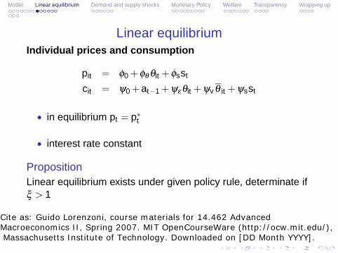
Linear equilibrium Individual prices and consumption
=pit φ0 + φθ θit + φsst
=cit ψ0 + at−1 + ψεθit + ψv θ it + ψsst
• in equilibrium pt = pt ∗
interest rate constant •
Proposition Linear equilibrium exists under given policy rule, determinate if ξ > 1
Cite as: Guido Lorenzoni, course materials for 14.462 Advanced Macroeconomics II, Spring 2007. MIT OpenCourseWare (http://ocw.mit.edu/), Massachusetts Institute of Technology. Downloaded on [DD Month YYYY].
Model Linear equilibrium Demand and supply shocks Monetary Policy Welfare Transparency Wrapping up
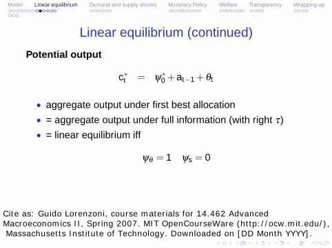
Linear equilibrium (continued)
Potential output
ct ∗ = ψ0
∗ + at−1 + θt
• aggregate output under first best allocation
• = aggregate output under full information (with right τ)
• = linear equilibrium iff
ψθ = 1 ψs = 0
Cite as: Guido Lorenzoni, course materials for 14.462 Advanced Macroeconomics II, Spring 2007. MIT OpenCourseWare (http://ocw.mit.edu/), Massachusetts Institute of Technology. Downloaded on [DD Month YYYY].
Model Linear equilibrium Demand and supply shocks Monetary Policy Welfare Transparency Wrapping up
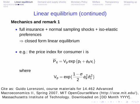
Linear equilibrium (continued) Mechanics and remark 1
• full insurance + normal sampling shocks + iso-elastic preferences
closed form linear equilibrium⇒
• e.g.: the price index for consumer i is
Pit = Vp exp{pt + φθ vi }
where
Vp = exp{ 1 −
2 σ
φθ 2σ̂ε
2}
Cite as: Guido Lorenzoni, course materials for 14.462 Advanced Macroeconomics II, Spring 2007. MIT OpenCourseWare (http://ocw.mit.edu/), Massachusetts Institute of Technology. Downloaded on [DD Month YYYY].
• → information structure is independent of monetary policy
Model Linear equilibrium Demand and supply shocks Monetary Policy Welfare Transparency Wrapping up
Linear equilibrium (continued)
Mechanics and remark 2
• consumers observe whole distribution Pjt for j ∈ Jit
• a sufficient statistic is θ it
• this is like having two noisy signals of θt :
θit = θt + εit
θ it = θt + vit
Cite as: Guido Lorenzoni, course materials for 14.462 Advanced Macroeconomics II, Spring 2007. MIT OpenCourseWare (http://ocw.mit.edu/), Massachusetts Institute of Technology. Downloaded on [DD Month YYYY].
Model Linear equilibrium Demand and supply shocks Monetary Policy Welfare Transparency Wrapping up
Linear equilibrium (continued) Mechanics and remark 2
• consumers observe whole distribution Pjt for j ∈ Jit
• a sufficient statistic is θ it
• this is like having two noisy signals of θt :
θit = θt + εit
θ it = θt + vit
information structure is independent of monetary policy • →
Cite as: Guido Lorenzoni, course materials for 14.462 Advanced Macroeconomics II, Spring 2007. MIT OpenCourseWare (http://ocw.mit.edu/), Massachusetts Institute of Technology. Downloaded on [DD Month YYYY].
� �
� � � �
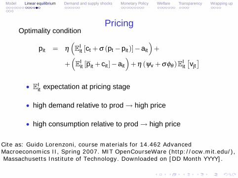
Model Linear equilibrium Demand and supply shocks Monetary Policy Welfare Transparency Wrapping up
Pricing Optimality condition
pit = η EitI [ct + σ (pt − pit )] − ait +
+ EIit [pit + cit ] − ait + η (ψv + σφθ )EI
it vjt
EIit expectation at pricing stage •
high demand relative to prod high price • →
• high consumption relative to prod high price →
Cite as: Guido Lorenzoni, course materials for 14.462 Advanced Macroeconomics II, Spring 2007. MIT OpenCourseWare (http://ocw.mit.edu/), Massachusetts Institute of Technology. Downloaded on [DD Month YYYY].
Cite as: Guido Lorenzoni, course materials for 14.462 Advanced Macroeconomics II, Spring 2007. MIT OpenCourseWare (http://ocw.mit.edu/), Massachusetts Institute of Technology. Downloaded on [DD Month YYYY].
����
Model Linear equilibrium Demand and supply shocks Monetary Policy Welfare Transparency Wrapping up
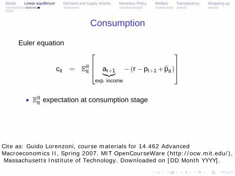
Consumption
Euler equation ⎡ ⎤
cit = EitII ⎣⎢ at+1 − (r − pt+1 + pit )⎦⎥
exp. income
• EitII expectation at consumption stage
Model Linear equilibrium Demand and supply shocks Monetary Policy Welfare Transparency Wrapping up
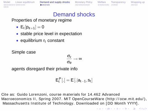
Demand shocks Properties of monetary regime
• Et [pit+1] = 0
• stable price level in expectation
• equilibrium rt constant
Simple case σε ∞σθ
→
agents disregard their private info
EP [.] = E [.|at−1,st ]t
Cite as: Guido Lorenzoni, course materials for 14.462 Advanced Macroeconomics II, Spring 2007. MIT OpenCourseWare (http://ocw.mit.edu/), Massachusetts Institute of Technology. Downloaded on [DD Month YYYY].
Model Linear equilibrium Demand and supply shocks Monetary Policy Welfare Transparency Wrapping up
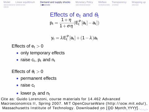
Effects of et and θt 1 + η
pt = 1 + ση
(EtP [at ] − at ])
yt = λ EP [at ]+ (1 − λ )att
Effects of et > 0
• only temporary effects
• raise ct , pt and nt
Effects of θt > 0
• permanent effects
• raise ct
• lower pt and nt
Cite as: Guido Lorenzoni, course materials for 14.462 Advanced Macroeconomics II, Spring 2007. MIT OpenCourseWare (http://ocw.mit.edu/), Massachusetts Institute of Technology. Downloaded on [DD Month YYYY].
0 2 4 6 8 100
0.02
0.04
0.06
0.08
0.1
y t
0 2 4 6 8 10-0.06
-0.04
-0.02
0
0.02
0.04
n t
0 2 4 6 8 10-0.04
-0.02
0
0.02
0.04
p t
0 2 4 6 8 100
0.02
0.04
0.06
0.08
0.1
a t|t
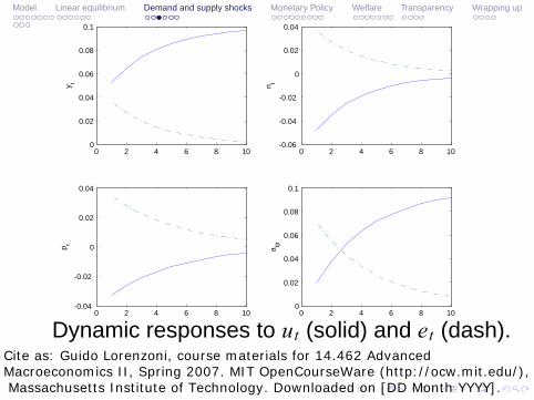
Dynamic responses to ut (solid) and et (dash).
Model Linear equilibrium Demand and supply shocks Monetary Policy Welfare Transparency Wrapping up
Cite as: Guido Lorenzoni, course materials for 14.462 Advanced Macroeconomics II, Spring 2007. MIT OpenCourseWare (http://ocw.mit.edu/), Massachusetts Institute of Technology. Downloaded on [DD Month YYYY].
Model Linear equilibrium Demand and supply shocks Monetary Policy Welfare Transparency Wrapping up
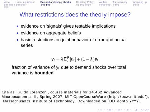
What restrictions does the theory impose?
• evidence on ’signals’ gives testable implications
• evidence on aggregate beliefs
• basic restrictions on joint behavior of error and actual series
= λ EP [at ]+ (1 − λ )atyt t
fraction of variance of yt due to demand shocks over totalvariance is bounded
Cite as: Guido Lorenzoni, course materials for 14.462 Advanced Macroeconomics II, Spring 2007. MIT OpenCourseWare (http://ocw.mit.edu/), Massachusetts Institute of Technology. Downloaded on [DD Month YYYY].
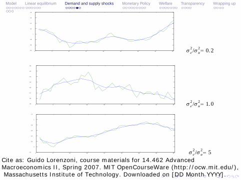
0 5 10 15 20 25 30 35 400.4
0.6
0.8
1
1.2
1.4
1.6
1.8
e2/u
2 0. 2
0 5 10 15 20 25 30 35 40-0.9
-0.8
-0.7
-0.6
-0.5
-0.4
-0.3
-0.2
e2/u
2 1. 0
0 5 10 15 20 25 30 35 40-0.2
0
0.2
0.4
0.6
0.8
1
1.2
e2/u
2 5
Model Linear equilibrium Demand and supply shocks Monetary Policy Welfare Transparency Wrapping up
Cite as: Guido Lorenzoni, course materials for 14.462 Advanced Macroeconomics II, Spring 2007. MIT OpenCourseWare (http://ocw.mit.edu/), Massachusetts Institute of Technology. Downloaded on [DD Month YYYY].
Model Linear equilibrium Demand and supply shocks Monetary Policy Welfare Transparency Wrapping up
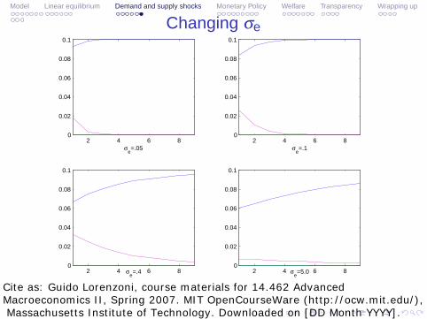
Changing σe
2 4 6 80
0.02
0.04
0.06
0.08
0.1
σe=.052 4 6 8
0
0.02
0.04
0.06
0.08
0.1
σe=.1
2 4 6 80
0.02
0.04
0.06
0.08
0.1
σe=.4 2 4 6 80
0.02
0.04
0.06
0.08
0.1
σe=5.0
Cite as: Guido Lorenzoni, course materials for 14.462 Advanced Macroeconomics II, Spring 2007. MIT OpenCourseWare (http://ocw.mit.edu/), Massachusetts Institute of Technology. Downloaded on [DD Month YYYY].
� �
Model Linear equilibrium Demand and supply shocks Monetary Policy Welfare Transparency Wrapping up
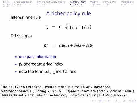
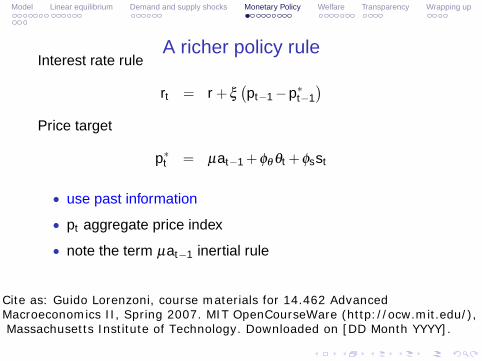
A richer policy rule Interest rate rule
rt = r + ξ pt−1 − pt ∗−1
Price target
pt ∗ = µat−1 + φθ θt + φsst
• use past information
• pt aggregate price index
• note the term µat−1 inertial rule
Cite as: Guido Lorenzoni, course materials for 14.462 Advanced Macroeconomics II, Spring 2007. MIT OpenCourseWare (http://ocw.mit.edu/), Massachusetts Institute of Technology. Downloaded on [DD Month YYYY].
Cite as: Guido Lorenzoni, course materials for 14.462 Advanced Macroeconomics II, Spring 2007. MIT OpenCourseWare (http://ocw.mit.edu/), Massachusetts Institute of Technology. Downloaded on [DD Month YYYY].
Model Linear equilibrium Demand and supply shocks Monetary Policy Welfare Transparency Wrapping up
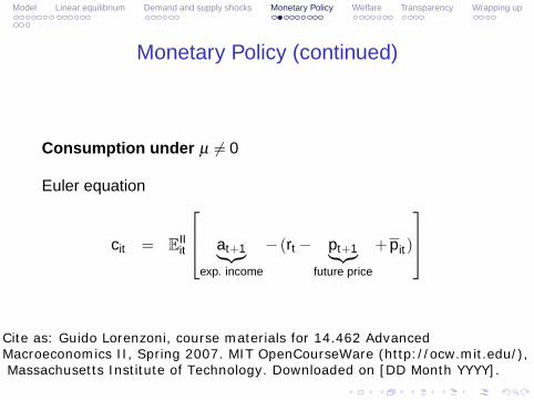
Monetary Policy (continued)
Consumption under µ =� 0
Euler equation ⎡ ⎤
cit EitII ⎢ − (rt − + pit )
⎥ = ⎣ at+1 pt+1 ⎦���� ���� exp. income future price
� �
Model Linear equilibrium Demand and supply shocks Monetary Policy Welfare Transparency Wrapping up
A richer policy rule Interest rate rule
rt = r + ξ pt−1 − pt ∗−1
Price target
pt ∗ = µat−1 + φθ θt + φsst
• use past information
• pt aggregate price index
• note the term µat−1 inertial rule
Cite as: Guido Lorenzoni, course materials for 14.462 Advanced Macroeconomics II, Spring 2007. MIT OpenCourseWare (http://ocw.mit.edu/), Massachusetts Institute of Technology. Downloaded on [DD Month YYYY].
Cite as: Guido Lorenzoni, course materials for 14.462 Advanced Macroeconomics II, Spring 2007. MIT OpenCourseWare (http://ocw.mit.edu/), Massachusetts Institute of Technology. Downloaded on [DD Month YYYY].
Model Linear equilibrium Demand and supply shocks Monetary Policy Welfare Transparency Wrapping up
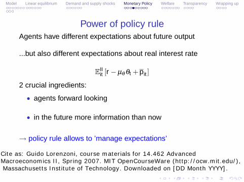
Power of policy rule Agents have different expectations about future output
...but also different expectations about real interest rate
EIIit [r − µθ θt + pit ]
2 crucial ingredients:
• agents forward looking
in the future more information than now •
policy rule allows to ’manage expectations’ →
Model Linear equilibrium Demand and supply shocks Monetary Policy Welfare Transparency Wrapping up
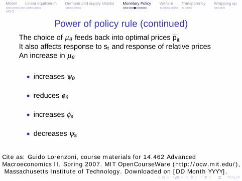
Power of policy rule (continued) The choice of µθ feeds back into optimal prices pit It also affects response to st and response of relative prices An increase in µθ
• increases ψθ
• reduces φθ
• increases φs
• decreases ψs
Cite as: Guido Lorenzoni, course materials for 14.462 Advanced Macroeconomics II, Spring 2007. MIT OpenCourseWare (http://ocw.mit.edu/), Massachusetts Institute of Technology. Downloaded on [DD Month YYYY].
Model Linear equilibrium Demand and supply shocks Monetary Policy Welfare Transparency Wrapping up
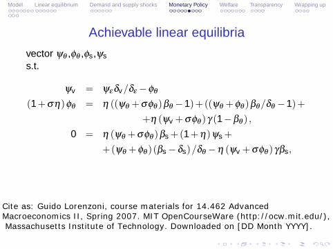
Achievable linear equilibria
vector ψθ ,φθ ,φs,ψs
s.t.
ψv = ψεδv /δε − φθ
(1 + ση)φθ = η ((ψθ + σφθ )βθ − 1)+((ψθ + φθ )βθ /δθ − 1)+
+η (ψv + σφθ )γ (1 − βθ ) , 0 = η (ψθ + σφθ )βs +(1 + η)ψs +
+(ψθ + φθ )(βs − δs)/δθ − η (ψv + σφθ )γβs,
Cite as: Guido Lorenzoni, course materials for 14.462 Advanced Macroeconomics II, Spring 2007. MIT OpenCourseWare (http://ocw.mit.edu/), Massachusetts Institute of Technology. Downloaded on [DD Month YYYY].
Model Linear equilibrium Demand and supply shocks Monetary Policy Welfare Transparency Wrapping up
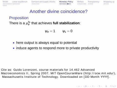
Another divine coincidence?PropositionThere is a µ
θ fs that achieves full stabilization:
ψθ = 1 ψs = 0
• here output is always equal to potential
• induce agents to respond more to private productivity
Cite as: Guido Lorenzoni, course materials for 14.462 Advanced Macroeconomics II, Spring 2007. MIT OpenCourseWare (http://ocw.mit.edu/), Massachusetts Institute of Technology. Downloaded on [DD Month YYYY].
0
0
1
μθ
ψθ
ψs
μθfs
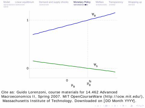
Figure 1: Monetary policy and aggregate stabilization.
4.4 Full stabilization
As noticed above, monetary policy can affect equilibrium behavior, but its scope is limited by the fact
that prices and consumption decisions are individually optimal. The following proposition shows that,
in spite of that, monetary policy can achieve full aggregate stabilization, that is, a path for aggregate
output, yt, which is identical to potential output, y∗t .
Proposition 5 There exist a subsidy, τfs, and a monetary policy rule, μfs, that, jointly, achieve fullaggregate stabilization, yt = y∗t . This corresponds to a linear equilibrium with parameters:
ψs = 0, ψθ = 1.
To illustrate this result Figure 1 shows the equilibrium relation between μθ and the parameters
(ψθ, , ψs). As discussed above, a positive value for μθ increases the response of the economy to the
fundamental shock. However, due to the equilibrium response of optimal prices, an increase in μθ also
reduces the response of the economy to the public signal. The surprising result is that when μθ = μfs
we reach an equilibrium where, at the same time, ψθ reaches 1 and ψs reaches 0.
13
Model Linear equilibrium Demand and supply shocks Monetary Policy Welfare Transparency Wrapping up
Cite as: Guido Lorenzoni, course materials for 14.462 Advanced Macroeconomics II, Spring 2007. MIT OpenCourseWare (http://ocw.mit.edu/), Massachusetts Institute of Technology. Downloaded on [DD Month YYYY].
Model Linear equilibrium Demand and supply shocks Monetary Policy Welfare Transparency Wrapping up
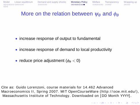
More on the relation between ψθ and φθ
• increase response of output to fundamental
• increase response of demand to local productivity
• reduce price adjustment (φθ < 0)
Cite as: Guido Lorenzoni, course materials for 14.462 Advanced Macroeconomics II, Spring 2007. MIT OpenCourseWare (http://ocw.mit.edu/), Massachusetts Institute of Technology. Downloaded on [DD Month YYYY].
� �
Model Linear equilibrium Demand and supply shocks Monetary Policy Welfare Transparency Wrapping up
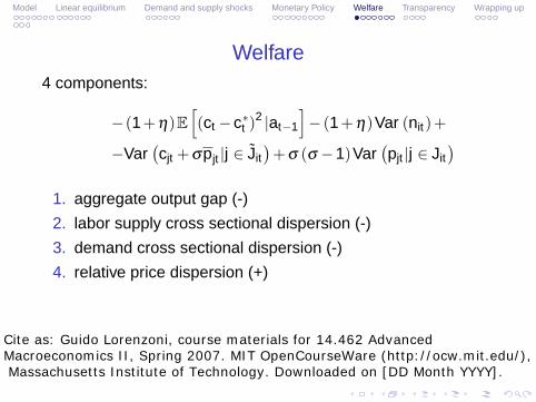
Welfare 4 components:
−(1 + η)E (ct − ct ∗)2 |at−1 − (1 + η)Var (nit )+
−Var � cjt + σpjt |j ∈ J̃it
� + σ (σ − 1)Var
� pjt |j ∈ Jit
�
1. aggregate output gap (-)
2. labor supply cross sectional dispersion (-)
3. demand cross sectional dispersion (-)
4. relative price dispersion (+)
Cite as: Guido Lorenzoni, course materials for 14.462 Advanced Macroeconomics II, Spring 2007. MIT OpenCourseWare (http://ocw.mit.edu/), Massachusetts Institute of Technology. Downloaded on [DD Month YYYY].
Cite as: Guido Lorenzoni, course materials for 14.462 Advanced Macroeconomics II, Spring 2007. MIT OpenCourseWare (http://ocw.mit.edu/), Massachusetts Institute of Technology. Downloaded on [DD Month YYYY].
Model Linear equilibrium Demand and supply shocks Monetary Policy Welfare Transparency Wrapping up
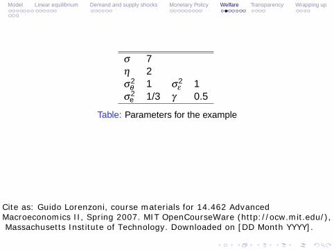
σ 7 η 2 σ
θ 2 1 σε
2 1 σ2 1/3 γ 0.5e
Table: Parameters for the example
-0.2 0 0.2 0.4 0.6 0.8 1 1.2-0.1
-0.05
0
-0.2 0 0.2 0.4 0.6 0.8 1 1.2-1
-0.5
0
-0.2 0 0.2 0.4 0.6 0.8 1 1.2
1
1.5
2
μθ
w1
w2,w3
w4
μθfs
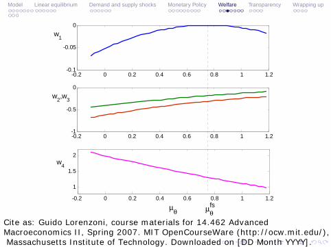
Figure 2: Monetary policy and welfare.
of prices observed by a given consumer, in particular the variance of the (log) prices in the basket of
consumer i is (1− γ) times the aggregate cross-sectional price variance. A value of 0.5 is chosen as a
conventional middle point.
σ 7η 2σ2θ 1 σ2 1σ2e 1/3 γ 0.5
Table 1: Parameters for the benchmark example
To illustrate the properties of optimal monetary policy Figure 2 plots the four elements in (12)
for this example. The first panel depicts w1, capturing the gains associated with the stabilization of
aggregate output. The maximum for this curve is reached at μfsθ , that is, at the point where aggregate
output is equal to potential. In accordance with Proposition 5, w1 is zero at μfsθ .
The effects on the remaining three components can be interpreted considering the effects of monetary
policy on equilibrium price dispersion. An increase in μθ, starting from the simple price-targeting rule,
μθ = 0, has the effect of reducing the dispersion of relative prices by reducing the value of |φθ|, whichdetermines the response of individual prices to individual productivity shock.15 This reduction in price
dispersion can be interepreted as follows. A household facing a positive productivty shock, θit > 0,
15Lemma ?? in the appendix shows that φθ < 0 as long as ψθ ≤ 1 and that the relation between μθ and φθ is monotone
15
Model Linear equilibrium Demand and supply shocks Monetary Policy Welfare Transparency Wrapping up
Cite as: Guido Lorenzoni, course materials for 14.462 Advanced Macroeconomics II, Spring 2007. MIT OpenCourseWare (http://ocw.mit.edu/), Massachusetts Institute of Technology. Downloaded on [DD Month YYYY].
-0.2 0 0.2 0.4 0.6 0.8 1 1.20.65
0.7
0.75
0.8
0.85
0.9
μθ
w
μθfsμθ
*
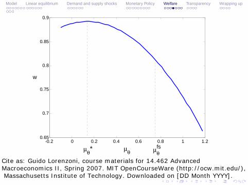
Figure 3: Optimal monetary policy
increases its consumption more if μθ > 0. As a consequence the incentive to increase labor effort is
dulled, and, at the price-setting stage, household i has a smaller incentive to reduce prices. Therefore,
relative prices respond less. This reduction in price dispersion has several effects. Given the assumptions
made about parameters it tends to reduce the dispersion in demand, although there is a countervailing
effect due to the fact that consumption is more responsive to the idiosyncratic shock. Moreover, it tends
to reduce the dispersion in labor supply. Both effects have positive welfare effects. This can be seen in
the second panel of Figure 2, where both curves w2 and w3 are increasing at μθ = 0. Finally, from the
point of view of the consumer, the reduction in price dispersion decreases welfare, as I argued above.
This effect is illustrated in the last panel curve of Figure 2.
In the example considered, the first component and the last component are the relevant ones from a
quantitative point of view. The optimal monetary policy μ∗θ balances the welfare costs of reducing pricedispersion, against the welfare gains of increasing aggregate volatility. As a consequence, μ∗θ is smallerthan μfsθ . In this case, it is optimal to reduce the aggregate volatility due to demand disturbances, but it
is not optimal to completely eliminate this source of volatility. This is illustrated in Figure 3 that plots
total welfare and shows that μ∗θ < μfsθ . Note that at the optimal monetary policy the corresponding
decreasing if the following inequality holds:
βθδθ+ ηβθ > ηγ (1− βθ)
µ1− δ
δθ
¶.
Both conditions are satisfied in this example, in a neighborhood of μθ = 0.
16
Model Linear equilibrium Demand and supply shocks Monetary Policy Welfare Transparency Wrapping up
Cite as: Guido Lorenzoni, course materials for 14.462 Advanced Macroeconomics II, Spring 2007. MIT OpenCourseWare (http://ocw.mit.edu/), Massachusetts Institute of Technology. Downloaded on [DD Month YYYY].
Model Linear equilibrium Demand and supply shocks Monetary Policy Welfare Transparency Wrapping up
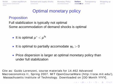
Optimal monetary policy
PropositionFull stabilization is typically not optimalSome accommodation of demand shocks is optimal
It is optimal µ∗ < µ fs •
• It is optimal to partially accomodate ψs > 0
• Price dispersion is larger at optimal monetary policy than under full stabilization
Cite as: Guido Lorenzoni, course materials for 14.462 Advanced Macroeconomics II, Spring 2007. MIT OpenCourseWare (http://ocw.mit.edu/), Massachusetts Institute of Technology. Downloaded on [DD Month YYYY].
Model Linear equilibrium Demand and supply shocks Monetary Policy Welfare Transparency Wrapping up
Special case
η = 0
• now it is optimal ψθ = 1
• φθ = −1
• decreasing prices proportionally to productivity gives:
1. right relative prices
2. right response of consumption
Cite as: Guido Lorenzoni, course materials for 14.462 Advanced Macroeconomics II, Spring 2007. MIT OpenCourseWare (http://ocw.mit.edu/), Massachusetts Institute of Technology. Downloaded on [DD Month YYYY].
� �
Model Linear equilibrium Demand and supply shocks Monetary Policy Welfare Transparency Wrapping up
Special case (continued)
=pit EiI [pit + cit ] − ait
cit = EiII [at+1 + pt+1] − pit
• unit intertemporal elasticity of substitution
• proportional response is optimal
Cite as: Guido Lorenzoni, course materials for 14.462 Advanced Macroeconomics II, Spring 2007. MIT OpenCourseWare (http://ocw.mit.edu/), Massachusetts Institute of Technology. Downloaded on [DD Month YYYY].

Model Linear equilibrium Demand and supply shocks Monetary Policy Welfare Transparency Wrapping up
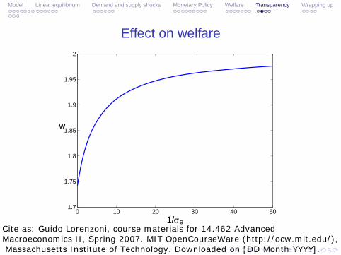
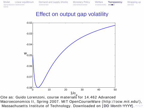
Transparency
Is better public information good? (Morris and Shin (2002))
• Effect on output gap may be bad
• Total effect always good
Cite as: Guido Lorenzoni, course materials for 14.462 Advanced Macroeconomics II, Spring 2007. MIT OpenCourseWare (http://ocw.mit.edu/), Massachusetts Institute of Technology. Downloaded on [DD Month YYYY].
Model Linear equilibrium Demand and supply shocks Monetary Policy Welfare Transparency Wrapping up
Effect on welfare
0 10 20 30 40 501.7
1.75
1.8
1.85
1.9
1.95
2
1/σe
w
Cite as: Guido Lorenzoni, course materials for 14.462 Advanced Macroeconomics II, Spring 2007. MIT OpenCourseWare (http://ocw.mit.edu/), Massachusetts Institute of Technology. Downloaded on [DD Month YYYY].
Model Linear equilibrium Demand and supply shocks Monetary Policy Welfare Transparency Wrapping up
Effect on output gap volatility
0 10 20 30 40 50-0.08
-0.07
-0.06
-0.05
-0.04
-0.03
-0.02
1/σe
w
Cite as: Guido Lorenzoni, course materials for 14.462 Advanced Macroeconomics II, Spring 2007. MIT OpenCourseWare (http://ocw.mit.edu/), Massachusetts Institute of Technology. Downloaded on [DD Month YYYY].
Model Linear equilibrium Demand and supply shocks Monetary Policy Welfare Transparency Wrapping up
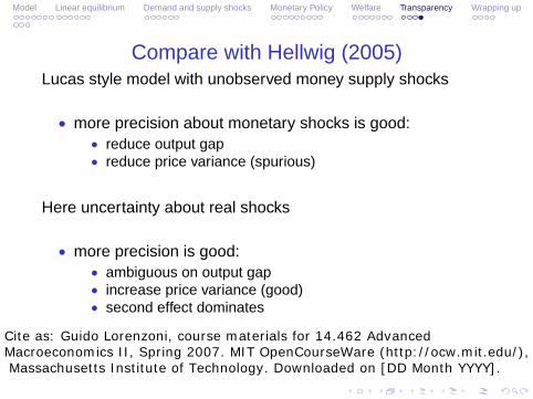
Compare with Hellwig (2005) Lucas style model with unobserved money supply shocks
• more precision about monetary shocks is good: • reduce output gap • reduce price variance (spurious)
Here uncertainty about real shocks
• more precision is good: • ambiguous on output gap • increase price variance (good)
second effect dominates•
Cite as: Guido Lorenzoni, course materials for 14.462 Advanced Macroeconomics II, Spring 2007. MIT OpenCourseWare (http://ocw.mit.edu/), Massachusetts Institute of Technology. Downloaded on [DD Month YYYY].
����
Model Linear equilibrium Demand and supply shocks Monetary Policy Welfare Transparency Wrapping up
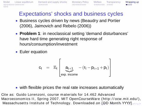
Expectations’ shocks and business cycles • Business cycles driven by news (Beaudry and Portier
(2006), Jaimovich and Rebelo (2006))
• Problem 1: in neoclassical setting ’demand disturbances’ have hard time generating right response of hours/consumption/investment
• Euler equation ⎡ ⎤
ct = Et ⎢⎣ at+1 − (rt − pt+1 + pt )
⎥⎦
exp. income
• with flexible prices the real rate increases automatically
Cite as: Guido Lorenzoni, course materials for 14.462 Advanced Macroeconomics II, Spring 2007. MIT OpenCourseWare (http://ocw.mit.edu/), Massachusetts Institute of Technology. Downloaded on [DD Month YYYY].
����
Model Linear equilibrium Demand and supply shocks Monetary Policy Welfare Transparency Wrapping up
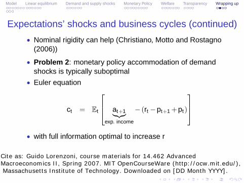
Expectations’ shocks and business cycles (continued)
• Nominal rigidity can help (Christiano, Motto and Rostagno (2006))
• Problem 2: monetary policy accommodation of demand shocks is typically suboptimal
• Euler equation ⎡ ⎤
ct = Et ⎢⎣ at+1 − (rt − pt+1 + pt )
⎥⎦
exp. income
• with full information optimal to increase r
Cite as: Guido Lorenzoni, course materials for 14.462 Advanced Macroeconomics II, Spring 2007. MIT OpenCourseWare (http://ocw.mit.edu/), Massachusetts Institute of Technology. Downloaded on [DD Month YYYY].
Model Linear equilibrium Demand and supply shocks Monetary Policy Welfare Transparency Wrapping up
Expectations’ shocks and business cycles (continued)
• Imperfect information + nominal rigidity can help
• Problem 3: policy rules still able to wipe out demand shocks
• ...but this is not optimal
• a theory of demand shocks that survive optimal policy
Cite as: Guido Lorenzoni, course materials for 14.462 Advanced Macroeconomics II, Spring 2007. MIT OpenCourseWare (http://ocw.mit.edu/), Massachusetts Institute of Technology. Downloaded on [DD Month YYYY].
• �
Model Linear equilibrium Demand and supply shocks Monetary Policy Welfare Transparency Wrapping up
Concluding • Future superior information + forward looking consumers
policy can induce efficient use of dispersed information →
• Related themes: King (1982), Svensson and Woodford (2003), Aoki (2003)
Efficient use of dispersed information = full stabilization output gap
• Still some offsetting of demand shocks is feasible and desirable
• Clearly this requires commitment, which may be tough (bubble example)
Cite as: Guido Lorenzoni, course materials for 14.462 Advanced Macroeconomics II, Spring 2007. MIT OpenCourseWare (http://ocw.mit.edu/), Massachusetts Institute of Technology. Downloaded on [DD Month YYYY].


![Preparation and characterization of very highly dispersed ... · pient wetness method resulted in well dispersed alumina-supported systems [16] but less well dispersed silica-supported](https://img.pdfslide.us/doc/110x75/5edc8590ad6a402d666736ef/preparation-and-characterization-of-very-highly-dispersed-pient-wetness-method.jpg)