Demand response strategies in residential buildings

Demand response strategies in residential buildings clusters to limit HVAC peak demand

Alice Mugnini1,*, Fabio Polonara1,2, and Alessia Arteconi3,1

1Università Politecnica delle Marche, Dipartimento di Ingegneria Industriale e Scienze Matematiche, Via Brecce Bianche 12, 60131, Ancona, Italy 2Consiglio Nazionale delle Ricerche, Istituto per le Tecnologie della Costruzione, Viale Lombardia 49, 20098, San Giuliano Milanese (MI), Italy 3KU Leuven, Department of Mechanical Engineering, B-3000, Leuven, Belgium

Abstract. Due to the increasing spread of residential heating systems electrically powered, buildings show a great potential in producing demand side management strategies addressing their thermal loads. Indeed, exploiting the intrinsic characteristics of the heating/cooling systems (i.e. the thermal inertia level), buildings could represent an interesting solution to reduce the electricity peak demand and to optimize the balance between demand and supply. The objective of this paper is to analyse the potential benefits that can be obtained if the electricity demand derived from the heating systems of a building cluster is managed with demand response strategies. A simulation-based analysis is presented in which a cluster of residential archetypal buildings are investigated. The buildings differ from each other for construction features and type of heating system (e.g. underfloor heating or with fan coil units). By supposing to be able to activate the energy flexibility of the single building with thermostatic load control, an optimized logic is implemented to produce programmatically an hourly electricity peak reduction. Results show how the involvement of buildings with different characteristics depends on the compromise that wants to be achieved in terms of minimization of both the rebound effects and the variation of the internal temperature setpoint.

1 Introduction To achieve the energy transition, there are two main objectives to be pursued: reducing

the energy consumption through energy efficiency policies and minimizing the use of fossil fuels. This entails the transition to a generation system based mainly on renewable sources. However, the most widespread among them (e.g. wind and photovoltaic) have an intermittent and hardly predictable nature which could undermine the security of energy supply.

One of the most promising solutions to improve the reliability of the energy supply is based on the development of policies aimed at making the energy system flexible. The idea is to make the energy demand adjustable depending on the availability of the generated

* Corresponding author: [email protected]

© The Authors, published by EDP Sciences. This is an open access article distributed under the terms of the Creative Commons Attribution License 4.0 (http://creativecommons.org/licenses/by/4.0/).

E3S Web of Conferences 312, 09001 (2021) https://doi.org/10.1051/e3sconf/20213120900176° Italian National Congress ATI

energy. Strategies to achieve such changes are known as Demand Side Management (DSM) [1]. Among them one of the most interesting programs is the Demand Response (DR). A DR event is defined as a mechanism aimed at producing changes in electric usage by end-use customers from their normal consumption patterns in response to changes in the price of electricity over time [2].

Buildings can play a very important role in enabling the implementation of such programs. The reasons are different. Firstly, they account for a very large proportion of total energy demand. It is estimated that they are responsible for around 33 % of the whole energy consumption [3]. In addition, thanks to the increasing use of electrically powered heating and cooling systems (i.e. heat pumps), it is also possible to benefit from the management of their thermal loads. This latter represents a great reserve of flexibility. Indeed, buildings have different ways to produce a decoupling between demand and generatio. The thermostatically controlled loads [4] can be exploited, or the thermal inertia of the thermal mass of the envelope [5] or of an added device as thermal energy storage [6] can be activated.

For all these reasons, the interest of the scientific community in assessing energy flexibility in buildings has grown more and more in recent years. For instance, Yongbao et. al. [7] summarized all the possible measured for improving the flexibility of commercial and residential buildings. In particular they identified five measures of flexibility: renewable energy to heating, ventilation, and air conditioning (HVAC) systems, energy storage, building thermal mass, appliances, and occupant behaviors. In addition Arteconi et al. [8] proposed a standard methodology to rate buildings according to their energy flexibility potential. With the calculation of a single indicator (the Flexibility Performance Indicator), they highlighted the different reserves of flexibility that buildings with different features in terms of construction characteristics and HVAC system can provide.

There are also many works that demonstrate the potential of buildings to operatively realize a DR events. An example is represented by the work proposed by D’Ettore et al. [9]. They investigated the flexibility potential associated with a building equipped with an optimally controlled hybrid generator (an electrically driven air source heat pump and a gas boiler) and a thermal energy storage under different demand response measures. In their results they showed how a high cost reduction associated with different DR actions can be obtained. It is between 45% and 75% in configuration with a Thermal Energy Storage (TES) of 0.5 m3 and between 50% and 78% for that with 0.75 m3.

These are just some examples of the many works available in the literature on the topic of energy flexibility in buildings. However, as Hu and Xiao [10] also point out, many of them relate to the assessment of the individual building. On the other hand, widening the context to the aggregated level may be fundamental to produce significant energy displacements and to reduce the undesirable effects (i.e., rebound effects) derived by a request for flexibility.

In a previous work, the authors began to approach this issue with an analysis that aimed to investigate the role of the differentiation of the users involved in a DR event [11]: the users were differentiated according to the occupancy profile patters. In this work the goal is to extend the analysis by considering the role of the construction characteristics (level of thermal insulation) and the type of heating system (thermal inertia levels provided) of buildings when they are involved in a DR event at the aggregate level.

Modeling a cluster of archetypal buildings [12], a peak shaving strategy is simulated as DR event. The energy flexibility of the individual users involved is activated allowing the variation of the internal temperature setpoint in a given band (flexibility of thermostatically controlled loads, TCLs). The way in which the individual buildings participate in the realization of the event is investigated. In this way it is possible to extrapolate guidelines for planning large-scale scenarios.

The paper is organized as follows. Section 2 describes the methodology followed to develop the model of the buildings’ clusters and to evaluate their behavior during an imposed

2


energy. Strategies to achieve such changes are known as Demand Side Management (DSM) [1]. Among them one of the most interesting programs is the Demand Response (DR). A DR event is defined as a mechanism aimed at producing changes in electric usage by end-use customers from their normal consumption patterns in response to changes in the price of electricity over time [2].

Buildings can play a very important role in enabling the implementation of such programs. The reasons are different. Firstly, they account for a very large proportion of total energy demand. It is estimated that they are responsible for around 33 % of the whole energy consumption [3]. In addition, thanks to the increasing use of electrically powered heating and cooling systems (i.e. heat pumps), it is also possible to benefit from the management of their thermal loads. This latter represents a great reserve of flexibility. Indeed, buildings have different ways to produce a decoupling between demand and generatio. The thermostatically controlled loads [4] can be exploited, or the thermal inertia of the thermal mass of the envelope [5] or of an added device as thermal energy storage [6] can be activated.

For all these reasons, the interest of the scientific community in assessing energy flexibility in buildings has grown more and more in recent years. For instance, Yongbao et. al. [7] summarized all the possible measured for improving the flexibility of commercial and residential buildings. In particular they identified five measures of flexibility: renewable energy to heating, ventilation, and air conditioning (HVAC) systems, energy storage, building thermal mass, appliances, and occupant behaviors. In addition Arteconi et al. [8] proposed a standard methodology to rate buildings according to their energy flexibility potential. With the calculation of a single indicator (the Flexibility Performance Indicator), they highlighted the different reserves of flexibility that buildings with different features in terms of construction characteristics and HVAC system can provide.

There are also many works that demonstrate the potential of buildings to operatively realize a DR events. An example is represented by the work proposed by D’Ettore et al. [9]. They investigated the flexibility potential associated with a building equipped with an optimally controlled hybrid generator (an electrically driven air source heat pump and a gas boiler) and a thermal energy storage under different demand response measures. In their results they showed how a high cost reduction associated with different DR actions can be obtained. It is between 45% and 75% in configuration with a Thermal Energy Storage (TES) of 0.5 m3 and between 50% and 78% for that with 0.75 m3.

These are just some examples of the many works available in the literature on the topic of energy flexibility in buildings. However, as Hu and Xiao [10] also point out, many of them relate to the assessment of the individual building. On the other hand, widening the context to the aggregated level may be fundamental to produce significant energy displacements and to reduce the undesirable effects (i.e., rebound effects) derived by a request for flexibility.

In a previous work, the authors began to approach this issue with an analysis that aimed to investigate the role of the differentiation of the users involved in a DR event [11]: the users were differentiated according to the occupancy profile patters. In this work the goal is to extend the analysis by considering the role of the construction characteristics (level of thermal insulation) and the type of heating system (thermal inertia levels provided) of buildings when they are involved in a DR event at the aggregate level.

Modeling a cluster of archetypal buildings [12], a peak shaving strategy is simulated as DR event. The energy flexibility of the individual users involved is activated allowing the variation of the internal temperature setpoint in a given band (flexibility of thermostatically controlled loads, TCLs). The way in which the individual buildings participate in the realization of the event is investigated. In this way it is possible to extrapolate guidelines for planning large-scale scenarios.

The paper is organized as follows. Section 2 describes the methodology followed to develop the model of the buildings’ clusters and to evaluate their behavior during an imposed

DR event. The case study is described in Section 3. In this section, a hypothetical cluster of archetypal buildings is selected. The results and their discussion are provided in Section 4 while in the last Section the main conclusions are summarized.

2 Methodology Following the cluster level assessments presented in [11], also in this paper a short-term

peak shaving event is modelled in the DR scenario. However more detailed building models representing archetypal buildings have been implemented in Python [13]. They are described in Section 2.1. For clarity in Section 2.2 a short description of the DR event modelling technique is repeated.

2.1 Building model

As for the single user model described in [11] also in this analysis a lumped-parameter model based on the thermal-electricity analogy is selected. However, to allow the modelling of different cases in terms of level and position of thermal insulation and type of heating system, more detailed models have been implemented.

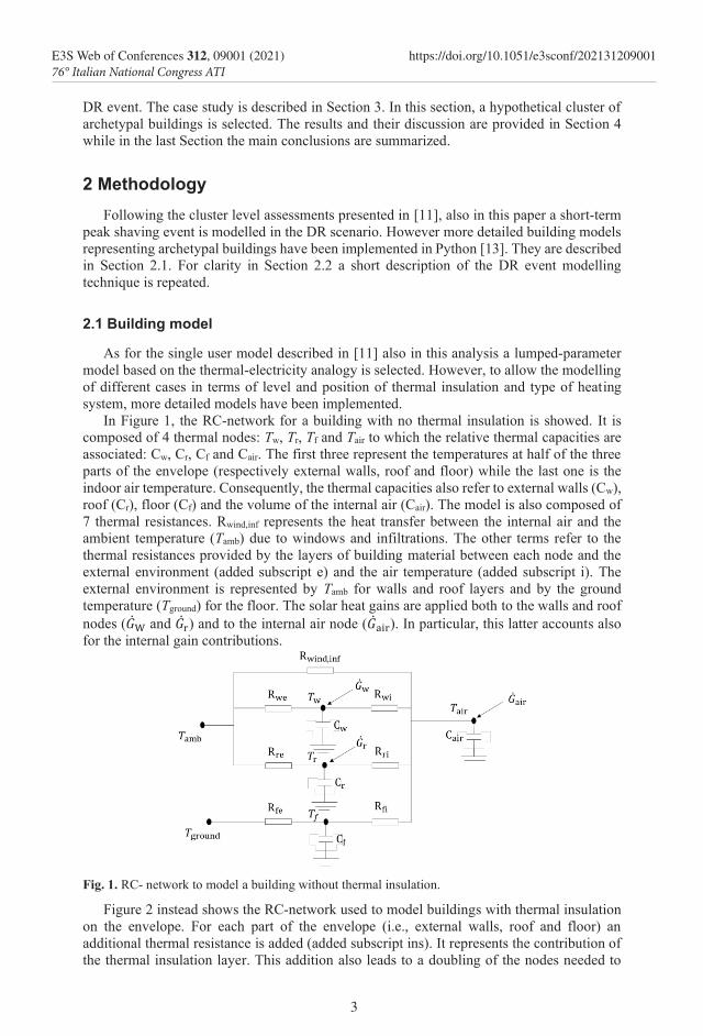
In Figure 1, the RC-network for a building with no thermal insulation is showed. It is composed of 4 thermal nodes: Tw, Tr, Tf and Tair to which the relative thermal capacities are associated: Cw, Cr, Cf and Cair. The first three represent the temperatures at half of the three parts of the envelope (respectively external walls, roof and floor) while the last one is the indoor air temperature. Consequently, the thermal capacities also refer to external walls (Cw), roof (Cr), floor (Cf) and the volume of the internal air (Cair). The model is also composed of 7 thermal resistances. Rwind,inf represents the heat transfer between the internal air and the ambient temperature (Tamb) due to windows and infiltrations. The other terms refer to the thermal resistances provided by the layers of building material between each node and the external environment (added subscript e) and the air temperature (added subscript i). The external environment is represented by Tamb for walls and roof layers and by the ground temperature (Tground) for the floor. The solar heat gains are applied both to the walls and roof nodes (��𝐺W and ��𝐺r) and to the internal air node (��𝐺air). In particular, this latter accounts also for the internal gain contributions.

Fig. 1. RC- network to model a building without thermal insulation.

Figure 2 instead shows the RC-network used to model buildings with thermal insulation on the envelope. For each part of the envelope (i.e., external walls, roof and floor) an additional thermal resistance is added (added subscript ins). It represents the contribution of the thermal insulation layer. This addition also leads to a doubling of the nodes needed to

3


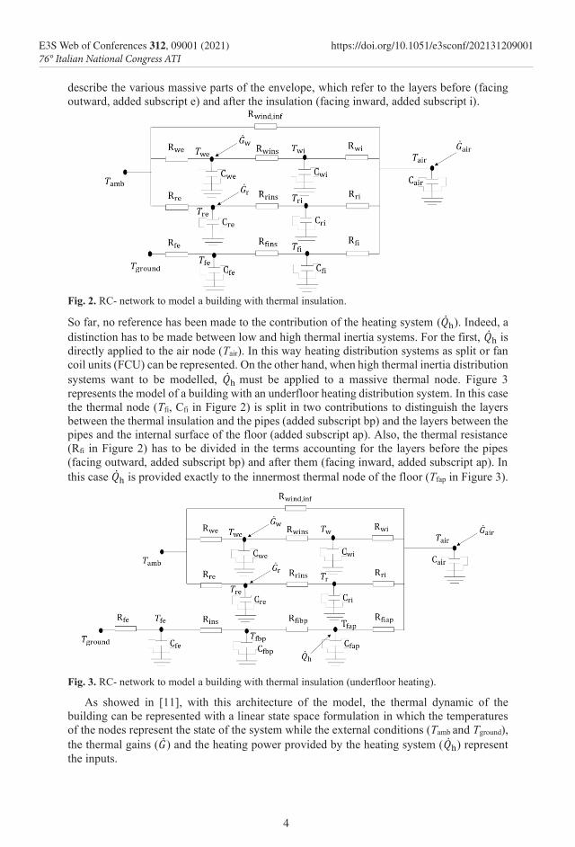
describe the various massive parts of the envelope, which refer to the layers before (facing outward, added subscript e) and after the insulation (facing inward, added subscript i).

Fig. 2. RC- network to model a building with thermal insulation.

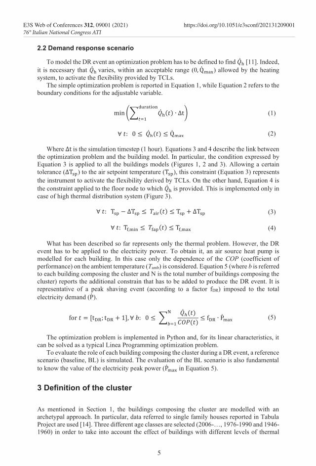
So far, no reference has been made to the contribution of the heating system (��𝑄h). Indeed, a distinction has to be made between low and high thermal inertia systems. For the first, ��𝑄h is directly applied to the air node (Tair). In this way heating distribution systems as split or fan coil units (FCU) can be represented. On the other hand, when high thermal inertia distribution systems want to be modelled, ��𝑄h must be applied to a massive thermal node. Figure 3 represents the model of a building with an underfloor heating distribution system. In this case the thermal node (Tfi, Cfi in Figure 2) is split in two contributions to distinguish the layers between the thermal insulation and the pipes (added subscript bp) and the layers between the pipes and the internal surface of the floor (added subscript ap). Also, the thermal resistance (Rfi in Figure 2) has to be divided in the terms accounting for the layers before the pipes (facing outward, added subscript bp) and after them (facing inward, added subscript ap). In this case ��𝑄h is provided exactly to the innermost thermal node of the floor (Tfap in Figure 3).

Fig. 3. RC- network to model a building with thermal insulation (underfloor heating).

As showed in [11], with this architecture of the model, the thermal dynamic of the building can be represented with a linear state space formulation in which the temperatures of the nodes represent the state of the system while the external conditions (Tamb and Tground), the thermal gains (��𝐺) and the heating power provided by the heating system (��𝑄h) represent the inputs.

4


describe the various massive parts of the envelope, which refer to the layers before (facing outward, added subscript e) and after the insulation (facing inward, added subscript i).

Fig. 2. RC- network to model a building with thermal insulation.

So far, no reference has been made to the contribution of the heating system (��𝑄h). Indeed, a distinction has to be made between low and high thermal inertia systems. For the first, ��𝑄h is directly applied to the air node (Tair). In this way heating distribution systems as split or fan coil units (FCU) can be represented. On the other hand, when high thermal inertia distribution systems want to be modelled, ��𝑄h must be applied to a massive thermal node. Figure 3 represents the model of a building with an underfloor heating distribution system. In this case the thermal node (Tfi, Cfi in Figure 2) is split in two contributions to distinguish the layers between the thermal insulation and the pipes (added subscript bp) and the layers between the pipes and the internal surface of the floor (added subscript ap). Also, the thermal resistance (Rfi in Figure 2) has to be divided in the terms accounting for the layers before the pipes (facing outward, added subscript bp) and after them (facing inward, added subscript ap). In this case ��𝑄h is provided exactly to the innermost thermal node of the floor (Tfap in Figure 3).

Fig. 3. RC- network to model a building with thermal insulation (underfloor heating).

As showed in [11], with this architecture of the model, the thermal dynamic of the building can be represented with a linear state space formulation in which the temperatures of the nodes represent the state of the system while the external conditions (Tamb and Tground), the thermal gains (��𝐺) and the heating power provided by the heating system (��𝑄h) represent the inputs.

2.2 Demand response scenario

To model the DR event an optimization problem has to be defined to find ��𝑄h [11]. Indeed, it is necessary that ��𝑄h varies, within an acceptable range (0, Qmax) allowed by the heating system, to activate the flexibility provided by TCLs.

The simple optimization problem is reported in Equation 1, while Equation 2 refers to the boundary conditions for the adjustable variable.

min (∑ ��𝑄h(𝑡𝑡) ∙ ∆tduration

𝑡𝑡=1) (1)

∀ 𝑡𝑡: 0 ≤ ��𝑄h(𝑡𝑡) ≤ Qmax (2)

Where ∆t is the simulation timestep (1 hour). Equations 3 and 4 describe the link between

the optimization problem and the building model. In particular, the condition expressed by Equation 3 is applied to all the buildings models (Figures 1, 2 and 3). Allowing a certain tolerance (∆Tsp) to the air setpoint temperature (Tsp), this constraint (Equation 3) represents the instrument to activate the flexibility derived by TCLs. On the other hand, Equation 4 is the constraint applied to the floor node to which ��𝑄h is provided. This is implemented only in case of high thermal distribution system (Figure 3).

∀ 𝑡𝑡: Tsp − ∆Tsp ≤ 𝑇𝑇air(𝑡𝑡) ≤ Tsp + ∆Tsp (3)

∀ 𝑡𝑡: Tf,min ≤ 𝑇𝑇fap(𝑡𝑡) ≤ Tf,max (4)

What has been described so far represents only the thermal problem. However, the DR

event has to be applied to the electricity power. To obtain it, an air source heat pump is modelled for each building. In this case only the dependence of the COP (coefficient of performance) on the ambient temperature (Tamb) is considered. Equation 5 (where b is referred to each building composing the cluster and N is the total number of buildings composing the cluster) reports the additional constrain that has to be added to produce the DR event. It is representative of a peak shaving event (according to a factor fDR) imposed to the total electricity demand (P).

for 𝑡𝑡 = [tDR; tDR + 1], ∀ 𝑏𝑏: 0 ≤ ∑��𝑄ℎ(𝑡𝑡)

𝐶𝐶𝐶𝐶𝐶𝐶(𝑡𝑡)

N

𝑏𝑏=1≤ fDR ∙ Pmax (5)

The optimization problem is implemented in Python and, for its linear characteristics, it

can be solved as a typical Linea Programming optimization problem. To evaluate the role of each building composing the cluster during a DR event, a reference

scenario (baseline, BL) is simulated. The evaluation of the BL scenario is also fundamental to know the value of the electricity peak power (Pmax in Equation 5).

3 Definition of the cluster

As mentioned in Section 1, the buildings composing the cluster are modelled with an archetypal approach. In particular, data referred to single family houses reported in Tabula Project are used [14]. Three different age classes are selected (2006-…, 1976-1990 and 1946-1960) in order to take into account the effect of buildings with different levels of thermal

5


insulation. Tables 1, 2 and 3 report the values of the thermal transmittances (U-values), surface area and the building structure for each part of the envelope suggested by Tabula for each archetype. Table 1. Description of the archetypal building with construction age 2006-… (SFH in Tabula Project).

Roof External walls Floor Windows U-values

(W m-2 K-1) 0.28 0.34 0.33 2.20

Area (m2) 96.4 223.3 96.4 21.7

Description

Ceiling with reinforced brick-

concrete slab, high insulation

Honeycomb bricks masonry (high

thermal resistance), high

insulation

Concrete floor on soil, high insulation

Low-e double glass, air or other gas filled, wood

frame

Table 2. Description of the archetypal building with construction age 1976-1990 (SFH in Tabula Project).


(W m-2 K-1) 1.14 0.76 0.76 2.80

Area (m2) 132.9 243.8 115.1 24.9

Description Pitched roof with

brick-concrete slab, low insulation

Hollow wall brick masonry (40 cm),

low insulation

Floor with reinforced brick-

concrete slab, low insulation

Double glass, air filled,

wood frame



(W m-2 K-1) 2.20 1.48 2.0 4.9

Area (m2) 97.6 232.1 84.6 20.3

Description Pitched roof with brick-concrete slab

Solid brick masonry (38 cm)

Concrete floor on soil

Single glass, wood frame

From the values reported in Tables 1, 2 and 3 the numerical values of the RC-networks parameters (Figures 1, 2 and 3) are identified with a white box approaches as showed in [15].

To model the variability of the external environment a climatic file is used and Rome, Italy (41°54’ N, 12°28' E), is selected as locality. According to [16], for a design outside temperature of 0 °C, a maximum heating load of 3.5 kWth is evaluated for the newest building (2006-…), 9.96 kWth for the archetypal building built between 1976-1990 and 15.4 kWth for the oldest archetypal building (1946-1960). These values are assumed as Qmax in Equation 2. Each archetypal building is modelled with a low thermal inertia heating system (i.e. FCU) according to the architectures showed in Figures 1 and 2. On the contrary, the high inertia distribution system (indicated with FLOOR) is applied only to the newest building (2006-…). Therefore, a cluster composed of 4 archetypal building is analysed.

The BL scenario is obtained with a fixed setpoint of 20 °C (Tsp in Equation 3) for each building composing the cluster (Equation 3). As far as the high inertia building is concerned, the numerical values of the floor node constraints expressed in Equation 4 are 18 °C for the

6


insulation. Tables 1, 2 and 3 report the values of the thermal transmittances (U-values), surface area and the building structure for each part of the envelope suggested by Tabula for each archetype. Table 1. Description of the archetypal building with construction age 2006-… (SFH in Tabula Project).


(W m-2 K-1) 0.28 0.34 0.33 2.20

Area (m2) 96.4 223.3 96.4 21.7

Description

Ceiling with reinforced brick-

concrete slab, high insulation

Honeycomb bricks masonry (high

thermal resistance), high

insulation

Concrete floor on soil, high insulation

Low-e double glass, air or other gas filled, wood

frame



(W m-2 K-1) 1.14 0.76 0.76 2.80

Area (m2) 132.9 243.8 115.1 24.9

Description Pitched roof with

brick-concrete slab, low insulation

Hollow wall brick masonry (40 cm),

low insulation

Floor with reinforced brick-

concrete slab, low insulation

Double glass, air filled,

wood frame



(W m-2 K-1) 2.20 1.48 2.0 4.9

Area (m2) 97.6 232.1 84.6 20.3

Description Pitched roof with brick-concrete slab

Solid brick masonry (38 cm)

Concrete floor on soil

Single glass, wood frame

From the values reported in Tables 1, 2 and 3 the numerical values of the RC-networks parameters (Figures 1, 2 and 3) are identified with a white box approaches as showed in [15].

To model the variability of the external environment a climatic file is used and Rome, Italy (41°54’ N, 12°28' E), is selected as locality. According to [16], for a design outside temperature of 0 °C, a maximum heating load of 3.5 kWth is evaluated for the newest building (2006-…), 9.96 kWth for the archetypal building built between 1976-1990 and 15.4 kWth for the oldest archetypal building (1946-1960). These values are assumed as Qmax in Equation 2. Each archetypal building is modelled with a low thermal inertia heating system (i.e. FCU) according to the architectures showed in Figures 1 and 2. On the contrary, the high inertia distribution system (indicated with FLOOR) is applied only to the newest building (2006-…). Therefore, a cluster composed of 4 archetypal building is analysed.

The BL scenario is obtained with a fixed setpoint of 20 °C (Tsp in Equation 3) for each building composing the cluster (Equation 3). As far as the high inertia building is concerned, the numerical values of the floor node constraints expressed in Equation 4 are 18 °C for the

minimum temperature (Tf,min) and 29 °C for the maximum (Tf,max). Instead, the DR scenario is evaluated with a setpoint tolerance of 1 °C (∆Tsp in Equation 3) for each building.

To model the dependence of the COP on the external air temperature data available for a commercial air source heat pump are used [17].

4 Results A representative day is selected to discuss the results. It is the day in which the average

temperature equals the average daily monthly temperature for the selected location. Since the analysis is realized for the heating season, the 23 January is selected (deviation from the average temperature less than 0.2 %).

To minimize the influence of the initial conditions imposed for the temperatures of the thermal nodes of RC-networks (Figures 1, 2 and 3), the solution of the optimization problem started on the previous day. This choice allows to evaluate also solutions in which the strategy of pre-heating (increase of the internal air temperature in the time before the event) can happen also for all the previous day. Even with this assumption, not all the possible load reduction events can be realized in the cluster. In fact, there is a limit to the value of fDR (Equation 5) due to the minimum thermal demand required to maintain the minimum setpoint of 19 °C during the event by buildings with low inertia heating system (i.e. FCU). This minimum value is assessed to be 48 % (fDR). Lower values of fDR in case of setpoint tolerance of 1 °C do not allow the optimization problem to find feasible solutions.

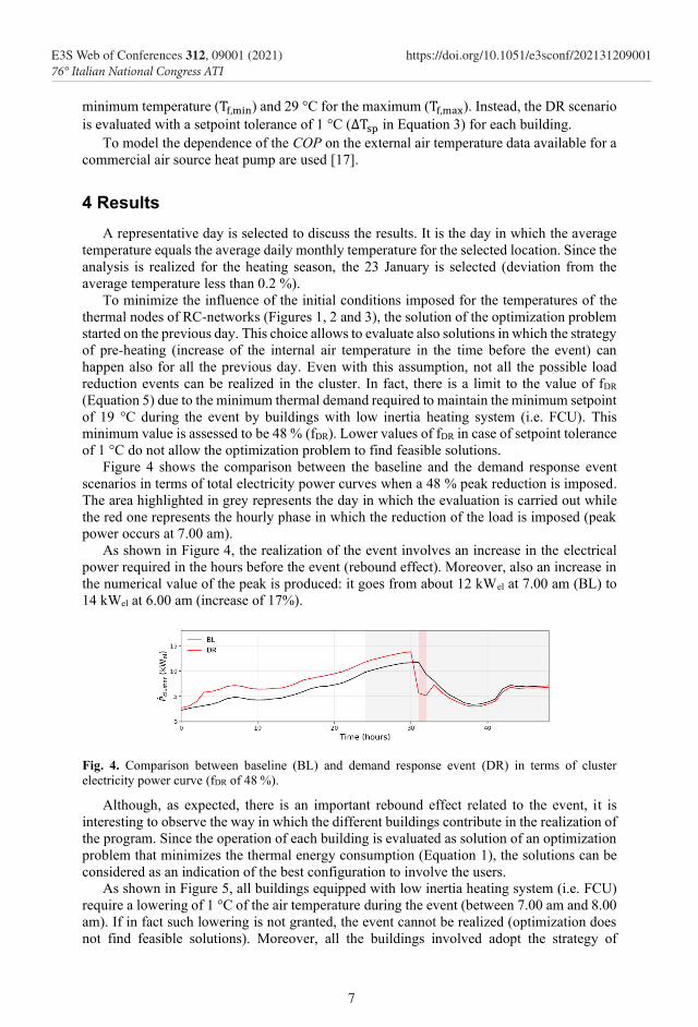
Figure 4 shows the comparison between the baseline and the demand response event scenarios in terms of total electricity power curves when a 48 % peak reduction is imposed. The area highlighted in grey represents the day in which the evaluation is carried out while the red one represents the hourly phase in which the reduction of the load is imposed (peak power occurs at 7.00 am).

As shown in Figure 4, the realization of the event involves an increase in the electrical power required in the hours before the event (rebound effect). Moreover, also an increase in the numerical value of the peak is produced: it goes from about 12 kWel at 7.00 am (BL) to 14 kWel at 6.00 am (increase of 17%).

Fig. 4. Comparison between baseline (BL) and demand response event (DR) in terms of cluster electricity power curve (fDR of 48 %).

Although, as expected, there is an important rebound effect related to the event, it is interesting to observe the way in which the different buildings contribute in the realization of the program. Since the operation of each building is evaluated as solution of an optimization problem that minimizes the thermal energy consumption (Equation 1), the solutions can be considered as an indication of the best configuration to involve the users.

As shown in Figure 5, all buildings equipped with low inertia heating system (i.e. FCU) require a lowering of 1 °C of the air temperature during the event (between 7.00 am and 8.00 am). If in fact such lowering is not granted, the event cannot be realized (optimization does not find feasible solutions). Moreover, all the buildings involved adopt the strategy of

7


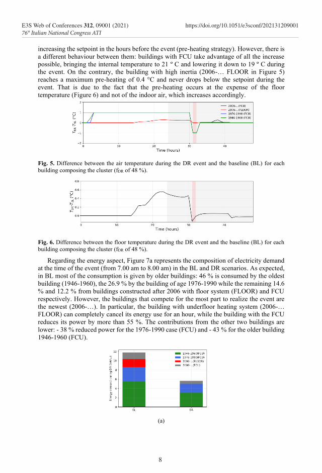
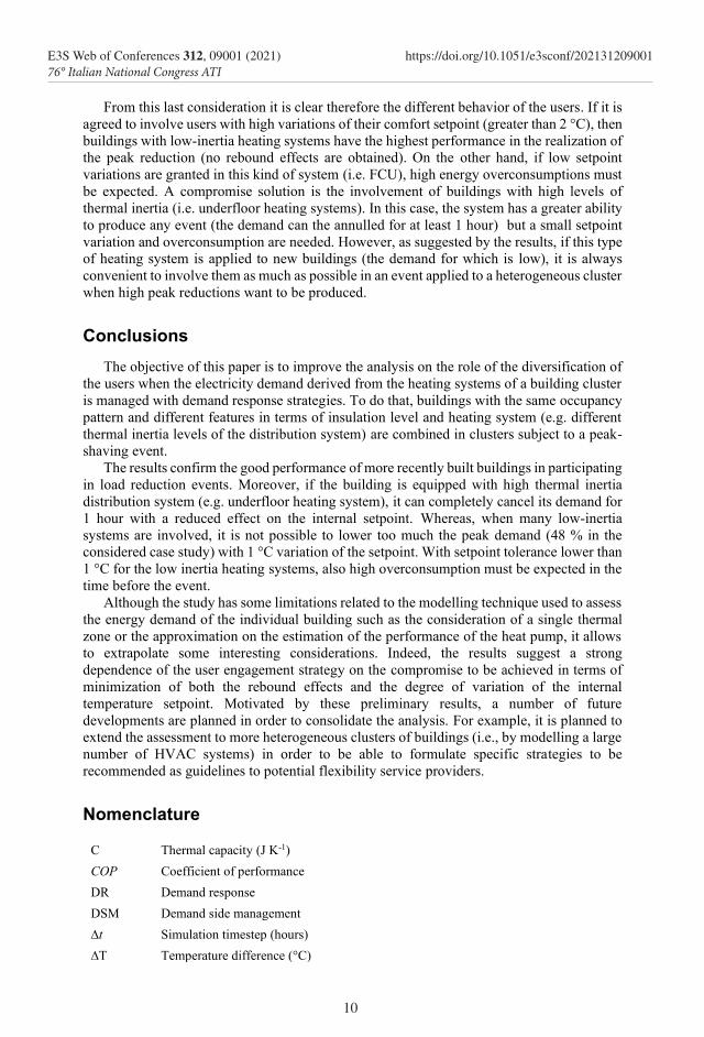
increasing the setpoint in the hours before the event (pre-heating strategy). However, there is a different behaviour between them: buildings with FCU take advantage of all the increase possible, bringing the internal temperature to 21 º C and lowering it down to 19 º C during the event. On the contrary, the building with high inertia (2006-… FLOOR in Figure 5) reaches a maximum pre-heating of 0.4 °C and never drops below the setpoint during the event. That is due to the fact that the pre-heating occurs at the expense of the floor temperature (Figure 6) and not of the indoor air, which increases accordingly.

Fig. 5. Difference between the air temperature during the DR event and the baseline (BL) for each building composing the cluster (fDR of 48 %).

Fig. 6. Difference between the floor temperature during the DR event and the baseline (BL) for each building composing the cluster (fDR of 48 %).

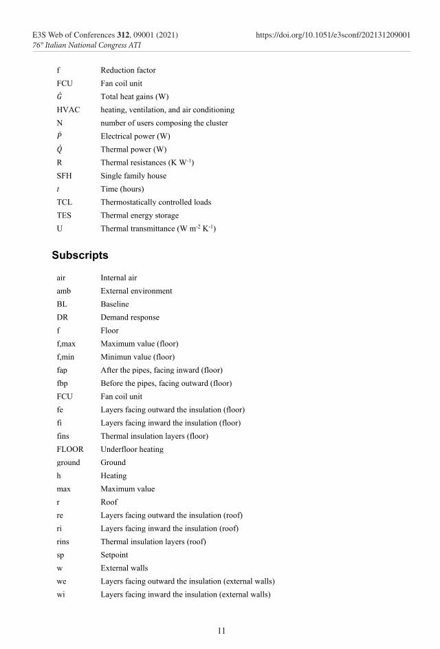
Regarding the energy aspect, Figure 7a represents the composition of electricity demand at the time of the event (from 7.00 am to 8.00 am) in the BL and DR scenarios. As expected, in BL most of the consumption is given by older buildings: 46 % is consumed by the oldest building (1946-1960), the 26.9 % by the building of age 1976-1990 while the remaining 14.6 % and 12.2 % from buildings constructed after 2006 with floor system (FLOOR) and FCU respectively. However, the buildings that compete for the most part to realize the event are the newest (2006-…). In particular, the building with underfloor heating system (2006-… FLOOR) can completely cancel its energy use for an hour, while the building with the FCU reduces its power by more than 55 %. The contributions from the other two buildings are lower: - 38 % reduced power for the 1976-1990 case (FCU) and - 43 % for the older building 1946-1960 (FCU).

(a)

8


increasing the setpoint in the hours before the event (pre-heating strategy). However, there is a different behaviour between them: buildings with FCU take advantage of all the increase possible, bringing the internal temperature to 21 º C and lowering it down to 19 º C during the event. On the contrary, the building with high inertia (2006-… FLOOR in Figure 5) reaches a maximum pre-heating of 0.4 °C and never drops below the setpoint during the event. That is due to the fact that the pre-heating occurs at the expense of the floor temperature (Figure 6) and not of the indoor air, which increases accordingly.

Fig. 5. Difference between the air temperature during the DR event and the baseline (BL) for each building composing the cluster (fDR of 48 %).

Fig. 6. Difference between the floor temperature during the DR event and the baseline (BL) for each building composing the cluster (fDR of 48 %).

Regarding the energy aspect, Figure 7a represents the composition of electricity demand at the time of the event (from 7.00 am to 8.00 am) in the BL and DR scenarios. As expected, in BL most of the consumption is given by older buildings: 46 % is consumed by the oldest building (1946-1960), the 26.9 % by the building of age 1976-1990 while the remaining 14.6 % and 12.2 % from buildings constructed after 2006 with floor system (FLOOR) and FCU respectively. However, the buildings that compete for the most part to realize the event are the newest (2006-…). In particular, the building with underfloor heating system (2006-… FLOOR) can completely cancel its energy use for an hour, while the building with the FCU reduces its power by more than 55 %. The contributions from the other two buildings are lower: - 38 % reduced power for the 1976-1990 case (FCU) and - 43 % for the older building 1946-1960 (FCU).

(a)

(b)

Fig. 7. Electricity demand composition in case of baseline (BL) and demand response (DR) scenarios: (a) focus in the hour of the event and (b) focus on the time before the event (fDR of 48 %).

Looking instead at the behavior in the hours before the event, Figure 7b compares the total consumption in the two scenarios distinguishing the contributions of the various buildings. It immediately appears as each plant increases its overall electricity consumption: + 42 % for 2006-... FCU, + 9 % for 2006-... FLOOR, + 31 % for 1976-1990 FCU and + 36 % for 1946-1960 FCU. Although the energy consumption of the newest buildings with FCU increases more than the other cases, they are only minimally responsible for the rebound effect in the total electricity power (Figure 4). Indeed, looking at Figure 8, in which the differences between DR and BL scenarios in term of electricity power consumption for each building involved are showed, it is possible to note that in terms of electric power the most important contributions are given by the older buildings.

Fig.8. Difference between electricity power curves during the DR event and in the baseline (BL) for each building composing the cluster (fDR of 48 %).

Results show that such rebound effects could be mitigated if higher tolerances are imposed on the setpoint during the event. If for example, the temperature is allowed to drop to 18 º C (∆Tsp in Equation 3) there is no excess of electricity (Figure 9). However, a high involvement of the users with low thermal inertia has to be taken into account.

Fig. 8. Comparison between baseline (BL) and demand response event (DR) in terms of cluster electricity power curve (fDR of 48 %, tolerance of 2 °C for the air temperature during the event).

9


From this last consideration it is clear therefore the different behavior of the users. If it is agreed to involve users with high variations of their comfort setpoint (greater than 2 °C), then buildings with low-inertia heating systems have the highest performance in the realization of the peak reduction (no rebound effects are obtained). On the other hand, if low setpoint variations are granted in this kind of system (i.e. FCU), high energy overconsumptions must be expected. A compromise solution is the involvement of buildings with high levels of thermal inertia (i.e. underfloor heating systems). In this case, the system has a greater ability to produce any event (the demand can the annulled for at least 1 hour) but a small setpoint variation and overconsumption are needed. However, as suggested by the results, if this type of heating system is applied to new buildings (the demand for which is low), it is always convenient to involve them as much as possible in an event applied to a heterogeneous cluster when high peak reductions want to be produced.

Conclusions The objective of this paper is to improve the analysis on the role of the diversification of

the users when the electricity demand derived from the heating systems of a building cluster is managed with demand response strategies. To do that, buildings with the same occupancy pattern and different features in terms of insulation level and heating system (e.g. different thermal inertia levels of the distribution system) are combined in clusters subject to a peak-shaving event.

The results confirm the good performance of more recently built buildings in participating in load reduction events. Moreover, if the building is equipped with high thermal inertia distribution system (e.g. underfloor heating system), it can completely cancel its demand for 1 hour with a reduced effect on the internal setpoint. Whereas, when many low-inertia systems are involved, it is not possible to lower too much the peak demand (48 % in the considered case study) with 1 °C variation of the setpoint. With setpoint tolerance lower than 1 °C for the low inertia heating systems, also high overconsumption must be expected in the time before the event.

Although the study has some limitations related to the modelling technique used to assess the energy demand of the individual building such as the consideration of a single thermal zone or the approximation on the estimation of the performance of the heat pump, it allows to extrapolate some interesting considerations. Indeed, the results suggest a strong dependence of the user engagement strategy on the compromise to be achieved in terms of minimization of both the rebound effects and the degree of variation of the internal temperature setpoint. Motivated by these preliminary results, a number of future developments are planned in order to consolidate the analysis. For example, it is planned to extend the assessment to more heterogeneous clusters of buildings (i.e., by modelling a large number of HVAC systems) in order to be able to formulate specific strategies to be recommended as guidelines to potential flexibility service providers.

Nomenclature

C Thermal capacity (J K-1) COP Coefficient of performance DR Demand response DSM Demand side management ∆t Simulation timestep (hours) ∆T Temperature difference (°C)

10


From this last consideration it is clear therefore the different behavior of the users. If it is agreed to involve users with high variations of their comfort setpoint (greater than 2 °C), then buildings with low-inertia heating systems have the highest performance in the realization of the peak reduction (no rebound effects are obtained). On the other hand, if low setpoint variations are granted in this kind of system (i.e. FCU), high energy overconsumptions must be expected. A compromise solution is the involvement of buildings with high levels of thermal inertia (i.e. underfloor heating systems). In this case, the system has a greater ability to produce any event (the demand can the annulled for at least 1 hour) but a small setpoint variation and overconsumption are needed. However, as suggested by the results, if this type of heating system is applied to new buildings (the demand for which is low), it is always convenient to involve them as much as possible in an event applied to a heterogeneous cluster when high peak reductions want to be produced.

Conclusions The objective of this paper is to improve the analysis on the role of the diversification of

the users when the electricity demand derived from the heating systems of a building cluster is managed with demand response strategies. To do that, buildings with the same occupancy pattern and different features in terms of insulation level and heating system (e.g. different thermal inertia levels of the distribution system) are combined in clusters subject to a peak-shaving event.

The results confirm the good performance of more recently built buildings in participating in load reduction events. Moreover, if the building is equipped with high thermal inertia distribution system (e.g. underfloor heating system), it can completely cancel its demand for 1 hour with a reduced effect on the internal setpoint. Whereas, when many low-inertia systems are involved, it is not possible to lower too much the peak demand (48 % in the considered case study) with 1 °C variation of the setpoint. With setpoint tolerance lower than 1 °C for the low inertia heating systems, also high overconsumption must be expected in the time before the event.

Although the study has some limitations related to the modelling technique used to assess the energy demand of the individual building such as the consideration of a single thermal zone or the approximation on the estimation of the performance of the heat pump, it allows to extrapolate some interesting considerations. Indeed, the results suggest a strong dependence of the user engagement strategy on the compromise to be achieved in terms of minimization of both the rebound effects and the degree of variation of the internal temperature setpoint. Motivated by these preliminary results, a number of future developments are planned in order to consolidate the analysis. For example, it is planned to extend the assessment to more heterogeneous clusters of buildings (i.e., by modelling a large number of HVAC systems) in order to be able to formulate specific strategies to be recommended as guidelines to potential flexibility service providers.

Nomenclature

C Thermal capacity (J K-1) COP Coefficient of performance DR Demand response DSM Demand side management ∆t Simulation timestep (hours) ∆T Temperature difference (°C)

f Reduction factor FCU Fan coil unit ��𝐺 Total heat gains (W) HVAC heating, ventilation, and air conditioning N number of users composing the cluster ��𝑃 Electrical power (W) ��𝑄 Thermal power (W) R Thermal resistances (K W-1) SFH Single family house t Time (hours) TCL Thermostatically controlled loads TES Thermal energy storage U Thermal transmittance (W m-2 K-1)

Subscripts

air Internal air amb External environment BL Baseline DR Demand response f Floor f,max Maximum value (floor) f,min Minimun value (floor) fap After the pipes, facing inward (floor) fbp Before the pipes, facing outward (floor) FCU Fan coil unit fe Layers facing outward the insulation (floor) fi Layers facing inward the insulation (floor) fins Thermal insulation layers (floor) FLOOR Underfloor heating ground Ground h Heating max Maximum value r Roof re Layers facing outward the insulation (roof) ri Layers facing inward the insulation (roof) rins Thermal insulation layers (roof) sp Setpoint w External walls we Layers facing outward the insulation (external walls) wi Layers facing inward the insulation (external walls)

11


wind,inf Windows and infiltrations wins Thermal insulation layers (external walls)

References

1. L. Gelazanskas K. A.A.Gamage, Demand side management in smart grid: A review

and proposals for future direction, Sustain Cities Soc, 11, 22–30 (2014) 2. R. Aazami, K. Aflaki, M. R. Haghifam, A demand response based solution for LMP

management in power markets, Int J Electr Power Energy Syst, 33, 125–1132 (2011) 3. IEA. Buildings. A source of enormous untapped efficiency potentia (2021) 4. D. Fischera, H. Madani, On heat pumps in smart grids: A review, Renew.

Sustain. Energy Rev, 70, 342-357 (2017) 5. S. Verbeke, A. Audenaert, Thermal inertia in buildings : A review of impacts across

climate and building use. Renew Sustain Energy Rev, 82, 2300–2318. (2020) 6. A. Arteconi, N.J. Hewitt, F. Polonara, Domestic demand-side management (DSM):

Role of heat pumps and thermal energy storage (TES) systems, Appl Therm Eng, 51, 155-165 (2013)

7. C. Yongbao, X. Peng, G. Jiefan, S. Ferdinand, L. Weilin. Measures to improve energy demand flexibility in buildings for demand response (DR): A review, Energy Build, 177, 125–139 (2018)

8. A. Arteconi, A. Mugnini, F. Polonara, Energy flexible buildings: A methodology for rating the flexibility performance of buildings with electric heating and cooling systems, Appl Energy, 251, 113387, (2019)

9. F. D’Ettorre, M. De Rosa, P. Conti, D. testi, D. Finn, Mapping the energy flexibility potential of single buildings equipped with optimally-controlled heat pump, gas boilers and thermal storage, Sustain Cities Soc, 50, 101689 (2019)

10. M. Hu, F. Xiao, Quantifying uncertainty in the aggregate energy flexibility of high-rise residential building clusters considering stochastic occupancy and occupant behavior, Energy, 194, 116838, (2020)

11. A. Mugnini, F. Polonara, A. Arteconi, Energy flexibility in residential buildings clusters, E3S Web Conf, 197, 10 (2020)

12. G. Buttitta, W. Turner, D. Finn, Clustering of Household Occupancy Profiles for Archetype Building Models, Energy Procedia, 111, 161-170 (2017)

13. M. Lutz, Learning Python, (2007) 14. V. Corrado, I. Ballarini, S.P. Corgnati. Typology Approach for Building Stock: D6.2

National scientific report on the TABULA activities in Italy (2012) 15. A. Mugnini, G. Coccia, F. Polonara, A. Arteconi, Energy Flexibility as Additional

Energy Source in Multi-Energy Systems with District Cooling, Energies, 14, 519 (2021)

16. UNI/TR, 10349-2. Heating and cooling of buildings - Climatic data - Part 2: Data for design load (2016)

17. Viessmann, VITOCAL 200-S AWB/AWB-AC 201.B04/ .B07/ .B10 / .B13 /.B16, Commercial datasheet catalogue (2017)

12


Documents

Demand response strategies in residential buildings