Demand for Post-compulsory Education: The Choice BetweenAcademic and Vocational Tracks∗

Cristina Lopez-Mayan†

CEMFI and UIMP

January 31, 2010

Abstract

I develop a discrete choice structural model of individual schooling decisions followingcompulsory education, to analyse the effect of expected life-time earnings. The model isestimated using Spanish data on educational histories. I study the two paths available toa Spanish young person considering post-compulsory education: academic high school andvocational high school. In my model the options open to an individual following completionof one of these two high school tracks are linked to their expected life-cycle earnings. Iuse the estimated model to assess how school attendance and dropout rates respond tochanges in expected earnings. I find that the largest impact in decreasing the dropout ratein post-compulsory high school is associated with raising the annual wage corresponding toa vocational diploma. I also find that the Spanish wage structure in 2006 discourages post-compulsory education attendance. It also affects the qualification of high school graduatesby reducing the share of workers with a vocational qualification.

Keywords: High school education, vocational education, expected life-cycle earnings, dropoutrate, discrete choice structural model, NPL algorithm.

JEL codes: I21, I28, J24.∗I would like to thank Manuel Arellano, Samuel Bentolila, Pedro Mira and Victor Aguirregabiria for very

helpful comments. Special thanks are also due to Dante Amengual, Laura Crespo, Laura Hospido and MichaelManove. I acknowledge financial support from Fundacion Ramon Areces. For the most recent version of thepaper, please see: http://www.cemfi.es/∼clopezmayan/†Contact: crislopezmaya@gmail.com

1

1 Introduction

This paper studies the effect of expected life-cycle earnings on schooling choices of Spanish youthfollowing compulsory education. To accomplish this, I formulate and estimate a sequential deci-sion model that accomodates the choices available to an individual after completing compulsoryschooling. Each year, the individual chooses the option that maximizes her expected life-timeutility. I use a rich microdataset on schooling histories elaborated by the Spanish StatisticsInstitute in 2005. This dataset has not been used for this purpose in previous research.

In the Spanish system, following compulsory schooling, the individual chooses between enter-ing the labor market and attending high school education. In the latter, she chooses between twopossible paths: vocational high school and academic high school. Individuals attend educationto accumulate completed grades towards the diploma. Graduation is a probabilistic outcomebecause, when the individual decides what option to choose, she faces uncertainty about theprobability of completing the grade. This probability depends on previous performance and onobserved individual characteristics.

Once the individual completes academic or vocational high school, she has available a newset of choices that include the option of entering the labor market and the option of continuing infurther education. In the latter case, the alternatives differ depending on the diploma obtained.I model the first decision following high school education because it is important in order tounderstand the preceding choices. For example, most individuals choose to attend academichigh school because this diploma is required to enter university. In my model, the optionsavailable to an individual following completion of one of the two high school tracks are alsolinked to their expected life-cycle earnings.

The contributions of this paper to the literature on human capital investment decisions aretwofold. This is the first time that a structural model on schooling decisions reflecting thedifferent tracks (academic and vocational) available in post-compulsory education is estimated.In addition, as suggested by human capital theory, the model establishes the link between thosedecisions and the expected life-time earnings corresponding to each of the options availablefollowing completion of these tracks. This model is of interest because it allows to quantifywhether changes in the expected life-time earnings generate changes in the track choice and/orin the dropout rate in (post-compulsory) high school education. This paper is the first studythat provides empirical evidence on these aspects.

From a methodological perspective, I estimate the model using Aguirregabiria and Mira(2002)’s nested pseudo likelihood algorithm (NPL), which allows the researcher to estimate dis-crete choice structural models without having to compute repeated solutions of the dynamic prob-lem. I assume that individuals finish compulsory schooling with differences in their preferencesand ability to progress in each track that influence subsequent choices. I follow a finite-mixture(nonparametric) approach to model this permanent unobserved heterogeneity. This assumptionimplies that the support points of the finite-mixture distribution and the probability of eachpoint are parameters to be estimated. This is the first time that the NPL algorithm is usedto estimate a finite horizon model with permanent unobserved heterogeneity where those masspoints and probabilities are estimated without imposing a distributional assumption1.

The estimated model is used to assess how individuals respond to a change in expected life-1Aguirregabiria and Mira (2007) implement the NPL in an infinite horizon model where they assume that

the only variable that presents permanent unobserved heterogeneity follows a discretized version of a Gaussianvariate with zero mean and constant variance. The support points are rescaled by the standard deviation and thedistribution is fully characterized by only estimating a single parameter.

2

cycle earnings. I make two types of exercises. The first one analyses how a separate changein the life-time earnings corresponding to university, vocational college, academic high school,vocational high school and compulsory schooling, respectively, affects schooling outcomes. Themain conclusion from these exercises is that the largest impact on the completion rate in uppersecondary education is found after an increase in the earnings received by workers with a voca-tional qualification. Increasing the annual wage of vocational college by ten percent every yearreduces the dropout rate by three percentage points. The decrease is uniquely driven by the lowerdropout rate in the technical track. This higher completion rate is accompanied by an increaseof fifteen percentage points in the proportion of individuals who decide to attend the vocationaltrack instead of the academic one. Moreover, these exercises also show that a ten percent in-crease in the life-cycle wages corresponding to compulsory schooling discourages participation inpost-compulsory education, reducing the attendance rate by six percentage points.

In the second type of exercises, I use the Spanish Wage Structure Survey of 2006 to showhow individuals would behave if they faced that wage structure in the moment they make theirschooling decisions. Except for university, the premium of each schooling level with respectto compulsory education decreased between 2002 and 2006. The model predicts that this wagestructure will discourage the participation in post-compulsory education, reducing the proportionof individuals who attend the technical track. Additionally, it will increase by almost eightpercentage points the dropout rate in this track. As a consequence, the proportion of individualswho have high school as their maximum education level will decrease. The evidence from theSpanish Labor Force Survey confirms this prediction. Among high school graduates, the sharewith a vocational diploma will be lower (from 19% in the baseline to 11%). So, there will bea change in the qualification of the high school graduates towards a reduction in the share ofworkers with a technical qualification.

The model of human capital investment assumes that the expected monetary reward drivesthe decision to invest in education. One issue that arises when testing the human capital modelis that earnings are only observed after the schooling investment has been completed. Whenindividuals make their education decisions, they face uncertainty about the wage they can earnfrom each choice. To deal with this issue, the literature uses two different approaches. The firstone assumes that individuals have rational expectations. This assumption implies that youthsknow their potential earnings profile and use it to predict their expected earnings. One of themost representative study using this approach is Willis and Rosen (1979). The second approach,suggested by Manski (1993), considers that young people form their expectations about theirpotential earnings observing the incomes realized by members of the preceding generations.

In this paper, I adopt the last approach and the reason is twofold. First, I consider that youngpeople do not form their expectations as the rational approach assumes. Instead, I consider theyobserve the wages of workers similar to them to predict the expected earnings associated to eacheducation level. Second, the dataset is short to observe individuals completing further educationfollowing high school education and working in the labor market. As a consequence, I assumethat youths observe the earnings of other individuals who are working in the moment they maketheir schooling decisions and use them, conditioned on some observed individual characteristics,to infer the life-cycle earnings of each schooling choice. The life-cycle profiles are constructedusing earnings from the Spanish Wage Structure Survey 2002. If the individual decides toattend further education following high school completion, the corresponding life-time earningsare weighted by the probability of graduation.

There are other papers that use the structural framework to analyse schooling decisions inpost-compulsory education but they only consider the choice between attending or dropping out

3

of high school, without distinguishing the kind of track. For example, Eckstein and Wolpin(1999) construct a model of high school progression where individuals can work and attendschool at the same time to analyse the effect of working on high school performance. Keaneand Wolpin (1997) formulate a model of occupation and schooling decisions in which individualsdecide among attending high school, staying at home and three occupation options.

Other papers, such as those by Arcidiacono (2004, 2005), analyse the decision of attendingcollege. However, unlike the model I present, they use a sample of high school graduates anddo not consider the link between the choice of attending college and the schooling decisions inthe high school level. Keane and Wolpin (1997) considers in some way this link because, intheir model, the individual can choose to attend education until she accumulates sixteen yearsof schooling and becomes a college graduate. However, they do not consider that there is uncer-tainty in the schooling progression and that the individual accumulates a complete grade justby attending school that year. Regarding this, I include uncertainty in the schooling progressionfollowing the approach of Eckstein and Wolpin (1999). In contrast, I model the first decisionfollowing high school completion while these authors assume that the value of the high schooldiploma embeds all the decisions about attending college.

There are other papers that analyse the decision between attending academic or vocationalhigh school but using a reduced-form approach. However, they do not analyse the effect ofthe expected life-time earnings on those decisions. For example, Bradley and Lenton (2007)analyses the effect of individual’s prior attainment, family background characteristics and stateof the labor market on the decisions of attending low and high levels of academic and vocationalhigh school and on the decision of entering the labor market. They find that individuals withthe best prior attainment enter high academic courses and are less likely to drop out while theleast qualified enroll in low level courses but are more likely to drop out. Using German data,Dustmann (2004) analyses the influence of parental background on the track that the childrenchoose when they finish primary school. In the German system the individual can choose amongthree paths: two are the basis for apprenticeship training and the third is the basis for attendinguniversity. He finds that parental background is strongly related to the track chosen by the childand, given the rigidity of the German education system to move among tracks, this translates insubstantial earnings differentials later in life.

The rest of the paper is organized as follows. The next section explains the Spanish educa-tion system. Section 3 presents the dataset and some descriptive statistics. Section 4 providesevidence on data correlations from reduced-form estimates. Section 5 presents the theoreticalmodel. Section 6 explains how the expected life-time earnings and the current wages includedin the model are computed. Section 7 explains the solution and estimation method. Section 8shows the parameter estimates and the model fit, and Section 9 presents the exercises used toquantify the impact of expected earnings on schooling choices. Finally, Section 10 concludes.

2 The Spanish education system

In the last decades, there has been a debate in Spain about the need to reform the educationsystem. This debate is motivated by the following facts:

• The Programme for the International Student Assessment (PISA) has shown that the per-formance of fifteen-year-old Spanish students is below the average of the OECD countries2.

2In the PISA study (OECD, 2003), the scores of Spain in maths, reading, science and problem solving were 485,481, 487 and 482 respectively, while the averages of the OECD countries were 500, 494, 500 and 500 respectively.

4

• There is a high proportion of individuals who drop out from both the compulsory and theupper secondary levels. As shown in Figure 1, these high dropout rates result in a highproportion of Spanish youths with compulsory schooling as their maximum educationallevel in comparison to other European countries. Only Malta and Portugal have higherpercentages than Spain.

Figure 1: Percentage of people aged 18-24 years old with at most compulsory schooling and whohave declared they are not receiving any education or training (2005). Source: Eurostat.

Of the 30.8% Spanish youths with at most compulsory schooling in 2005, 19% have onlyprimary education (MEC, 2006). Thus, this group contains individuals who dropped out ofcompulsory education. The rest (81%) have compulsory schooling. This second category includesindividuals who entered the labor market after finishing compulsory schooling and individualswho started in upper secondary education but dropped out.

Education in Spain is run by regional governments. However, the central government estab-lishes some general aspects that have to be applied in all the territory of Spain: compulsoryschooling age, schooling levels, basic content of the curriculum, number of pupils per class, etc.

Both compulsory and (post-compulsory) high school education are public and free althoughthe individual can choose to attend education in private and semi-private schools (colegios con-certados). Private schools are more expensive than semi-private ones because the latter receivegovernment subsidies.

The education law relevant for the schooling decisions analyzed in this paper was the lawpassed in 19903 and that regulated the Spanish education system until 2006. One of the most

3Ley Orgánica 1/1990 de Ordenación General del Sistema Educativo (LOGSE).

5

important changes introduced by this law was the increase of the minimum compulsory schoolingage from fourteen to sixteen years old.

Figure 2 represents the schooling levels. Compulsory schooling attendance covers ten years,

Figure 2: Schooling levels

up to the age of sixteen. If the individual passes all grades, she gets the compulsory diploma.The law establishes that the individual can fail up to two grades in this stage. In case she failsmore than twice, she has to leave school and pass an official test provided by the administrationto obtain the compulsory education certificate.

The next schooling level is upper secondary or high school education. It is non-compulsoryand the only requirement to start in this level is to have the compulsory diploma. In this stage,the individual can choose between attending academic high school and vocational high school4.

Academic high school has two grades, from sixteen to eighteen years old. The law establishesa maximum of four years for graduation. That is, it allows the individual to fail up to twice. Ifshe fails more times, she has to leave the school and pass a test provided by the administrationin order to get the academic high school diploma.

The education received by the student in the academic high school is more specific than inthe previous level and it is predominantly oriented to the access to the tertiary level (mainlyuniversity attendance).

Since the first grade, the individual has to choose one program among four different possi-bilities: social sciences and humanities, arts, health and natural sciences, and technology. Inaddition to the program-specific subjects, all the students have several common subjects.

Access to the second grade requires that the number of failed subjects is equal to or less thantwo. Otherwise, the individual has to repeat the complete grade. Graduation from academichigh school requires to have passed all the subjects both from the first and the second grades.

Vocational education in Spain is a schooling-based training with apprenticeship in firms up totwenty-five percent of the total time of the program. Depending on the program, the vocationaltrack can have one or two grades. The individual can choose among a wide range of technical

4Individuals without the compulsory diploma and, at least with 18 years old, can attend vocational high schoolif they previously pass a test provided by the regional administration.

6

programs.Training is oriented to give an individual a specific qualification for the access to the labor

market. The kind of occupations that individuals have access to with a technical qualification aremainly blue-collar occupations (such as machinery mechanics and repairers; electronics mechanicsand servicers; agricultural, forestry and fishery labourers,...) but also some white-collar jobs (suchas clerical workers or sales workers).

The law allows to switch between academic and vocational high school. Depending on theorigin and destination tracks, it is possible to waive some subjects.

After graduation in academic or vocational high school, the individual can attend tertiaryeducation. In Spain, there are two possibilities at this level: university and vocational college.Access to university requires the academic high school diploma but this is only a sufficientcondition. It is also necessary to pass a general (not university-specific) test that determines,jointly with the average grade in the academic track, the final grade to apply for admission in auniversity field.

The academic high school diploma also allows access to vocational college and, unlike foruniversity, the individual does not have to take any admission test (although it could be requiredthat the academic program is related to the field chosen in vocational college).

In order to enter vocational college with a technical high school diploma, the individual hastwo options: to validate the technical program with an academic program and, so, to get theacademic high school diploma, or if she is eighteen or older, that validation process can besubstituted by an admission test.

Following completion of the academic track, an individual can start in the vocational trackand viceversa (an individual can attend academic high school following completion of a technicalprogram).

3 The data

The data used in this paper come from a survey produced by the Spanish Statistics Institute in2005, Encuesta de Transición Educativo-Formativa e Inserción Laboral (ETEFIL). The objectiveof this survey is to know the education and labor decisions of individuals who graduate from anynon-university education level in the school year 2000/2001. Specifically, the sampled groups areindividuals who complete in 2000/2001:

• Compulsory education.

• Academic high school.

• Vocational high school.

• Vocational college.

Additionally to these four groups, individuals who dropped out of compulsory education in2000/2001 are also sampled.

For each of these groups, samples are obtained using a stratified two-step method: firststep units are schools and second step units are pupils. Information is collected through aretrospective interview: individuals are asked about their education decisions and labor activitiessince 2000/2001 until the moment of the interview (May-July 2005). So, the dataset containsfour observations for each individual (one by year).

7

In this paper, I restrict my attention to the sample of individuals who obtained the compul-sory diploma in 2000/2001 (8098 individuals). It covers the period corresponding to the uppersecondary education and it also covers one or two years following high school completion. Forexample, individuals who obtained an academic high school diploma in two years (therefore,without failing any grade) are observed two years in the option they chose following graduation.Only the individuals who graduated in the last year are right-censored in their next decision butthey represent a small percentage of the total sample as I will show below.

The data contain three kinds of information:

- Personal characteristics. Individuals are asked about their date of birth, gender, na-tionality, mother and father’s education and region of residence.

- Education. With respect to the compulsory level, individuals report the age at whichthey obtained the compulsory diploma and whether they attended a private, semi-privateor public school. With respect to the post-compulsory levels, year by year the survey askswhether the individual decided to leave the school or to attend education. In the first case,the individual reports the leaving-school dates. In the second case, she is asked about thekind of track she chose, the grade and the program she attended and whether or not shegraduated that year. The individual also indicates whether she attended a private or publicschool and whether she has changed to a new school in the current year. Individuals alsoreport their decision following completion of high school education.

- Work. On a monthly basis, all individuals are asked about their employment or unemploy-ment status. If they work, they report whether the job is part-time or full-time. A detailedquestionnaire on the job/unemployment characteristics is asked to those individuals whoare in some of the following situations:

1. They work in a full-time job or they are unemployed in the moment of the interview.

2. They worked in a full-time job in the same firm or they were unemployed for at leastsix consecutive months in the past.

Individuals have to fill in as many questionnaires as times they are in any of the previoussituations.

The questions about the job refer to the activity of the firm, occupation, net monthlywage in an interval basis, type of contract, hours worked, necessary qualification in the job,starting and finishing dates, the means that the individual used to find the job and thereason why the individual left the job (only for jobs in the past).

The questionnaire for the unemployment situation asks about the means that the individualuses to search for a job, whether she receives unemployment benefits, the starting andfinishing dates of the unemployment spell and whether she received any job offer.

One piece of information not included in the database is individual subject grades bothfor the compulsory and post-compulsory levels. With respect to the lack of an average gradefor compulsory schooling, the database contains the age at which the individual finished thecompulsory schooling and this variable can be used as a proxy for her performance because,generally, repeating will be the main reason to finish with more than sixteen years old5.

5Other explanations such as moving to a new city or being sick for a long time could also be possible butinfrequent.

8

The absence of grades from academic and vocational high school, in principle, could be alimitation to construct the individual grade level progression. However this is not the casebecause from the data it is possible to infer whether an individual passed a grade or, on thecontrary, she failed and had to repeat in the next year. Since attainment of a high school diplomaonly requires accumulation of grades (it is not necessary to achieve any average grade requisite),I consider that the information in the data captures the most essential features of the grade levelprogression. In appendix A, I explain how I construct the individual grade level progression andTable A1 shows the percentage of individuals who pass a grade in each school-year and in eachtrack.

3.1 Descriptive statistics

From the initial sample, I decide to drop some individuals (see appendix A) remaining a samplewith 7945 individuals. As I mentioned previously I observe the decisions following completion ofupper secondary education for almost all individuals. There are only 195 individuals (2.45% ofthe selected sample) who are right-censored because they graduate at the end of the academicyear 2004/2005. Due to the censoring, these individuals are excluded from the sample used toestimate the model. This finally contains 7750 individuals.

Following compulsory education, the individual can decide to attend the academic track orthe vocational track. Regarding this, obtaining a technical diploma can require to pass one ortwo grades depending on the kind of program attended. Those individuals who not attend schoolcan stay at home or enter the labor market. Each year, I decide to group the decisions followingcompulsory schooling in four categories: academic high school, one-grade vocational high school,two-grades vocational high school and labor market. The first three correspond to the decision ofattending the academic track or the vocational track of one or two grades respectively. The lastcategory includes individuals who not attend school that year. In order to simplify the analysis,I do not consider to stay at home as a separate category. Instead, I assume that all individualswho not attend school participate in the labor market. This is not a restrictive assumption giventhat most individuals who not attend school are observed working at least one month during theschool months (see column fifth in Table 8).

Now I comment some descriptive aspects of the sample. All the percentages are calculatedusing the population weights provided by the database.

Table 1 shows several data distributions conditioning on different characteristics. In the firstrow we can see that more than half of the individuals who graduated from compulsory educationare females. The next rows show the distribution of individuals by the age at which they obtainedthe compulsory diploma. Around 19% and 8% of the individuals finished with one and two yearsof delay, respectively. Table 2 below shows that among males the percentage that graduatedwith delay is higher than among females.

The next rows of table 1 show that most individuals attended compulsory education in apublic school and only 5% went to a private school. With respect to parents’ education, morethan 40% of the parents have compulsory education, around 8% of them have some kind ofvocational diploma and between 15-18% have a university degree. Fathers always present highereducation than mothers. The last rows of the table show the distribution of the programs chosenin academic and vocational high school, respectively.

Table 3 contains the choice distribution by school-year with respect to the total number ofindividuals who start that year without having completed upper secondary education previously.The first important fact is that just after finishing compulsory education 80% of the individuals

9

choose academic high school while only 15% choose the vocational track. And only 5% of themleave education altogether.

In the second year following compulsory schooling, there is a small increase in the percentagewho chooses labor market reflecting the fact that some individuals decided to drop out after oneyear in upper secondary education. Between the second and the third year, however, there is animportant decrease in the percentage choosing the academic track. Graduation from academichigh school takes two years and by the begining of the school-year 2003/04 many individualshave graduated. Most of the non-graduated individuals will have to repeat a complete grade inthat year. On the other hand, some individuals in the vocational track also graduated at the endof the second year. The fact that the percentage of the labor market option increases and thatthe percentage choosing vocational high school is almost constant reflects that many individualsdropped out of or transferred from the academic to the vocational track in the year three. Inthe last year, the situation is very similar to the previous one but with a higher percentage inlabor market, reflecting again the dropping out of both types of tracks.

The decisions present differences by gender. The proportion of males who choose vocationaland academic high school is 56.57% and 43.61%, respectively. These differences by gender areclearly reflected in Table 4. Around 83% of females chose the academic track just after gettingthe compulsory diploma and only 11% of them chose vocational high school. However, amongmales, 18% decided to enroll in vocational education.

Table 4 also reflects that the decisions following compulsory education are very different bythe age at which the individual graduated: 91% of individuals who finished with sixteen yearsold entered academic high school while this percentage is lower among individuals who finishedwith delay, (specially for people with two years of delay).

Table 5 shows the transition matrices. They provide evidence of persistence in decisions.Each matrix indicates the one-period transition rates, that is, the percentage of transitions fromorigin (decision in year t−1) to destination (decision in year t). The transitions in the first threematrices are calculated over the total number of individuals who start the school-year t withouthaving completed high school education (7627, 3045 and 1814 individuals respectively). The lastmatrix is calculated over the total number of observations in each transition across years (12486observations).

The general conclusion from Table 5 is that there is a strong state dependence in data,especially in academic high school and labor market options. This means that most individualswho choose an option in year t− 1 stay in the same option in year t. This persistence decreasesacross time for academic and vocational high school and remains more constant for the labormarket option (except in the third transition in which the persistence increases). The strongstate dependence in the labor market option implies that reenrollment after a period working isa rare event.

The transitions between the academic and the vocational tracks are not very frequent. Around4% of those individuals who attend the academic track one year decide to change to the technicaltrack in the next year. The transition from vocational to academic high school is even lessfrequent except between 2003/04 and 2004/05. The transitions from schooling options to labormarket increase across years and they are higher in the case of vocational high school. Thesetransitions reflect the dropout decisions.

By the moment of the interview (four years following completion of compulsory education)24% of the individuals do not have a high school diploma. This rate varies by the delay infinishing compulsory schooling. It is 15% among individuals who finished compulsory schoolingwith sixteen years old and 43% and 55% among individuals who finished with one and two

10

years of delay, respectively. That 24% includes both individuals who never participate in uppersecondary education and individuals who participate but drop out.

Table 6 contains the graduation rates. They are computed as the rate of graduated overenrolled individuals (so, the counterpart are the dropout rates). For the total sample, thegraduation rate is 80.07%. So, almost 20% dropped out of upper secondary education. Bytracks, the completion rate in academic high school is higher than in the vocational track. And,again, there are differences by gender: females have a higher rate than males in both tracks (thebiggest difference is 10.54 percentage points in vocational high school).

Among all the individuals who complete a high school track, 17.31% obtained a technicaldiploma. Table 7 presents the distribution of the decisions following completion of each track.According to the Spanish system, with an academic diploma it is possible to choose amonguniversity, vocational college, vocational high school or entering the labor market. As we cansee in Table 7 the most chosen option is university (73%) followed by vocational college (19%).With a technical diploma, the available options are vocational college, academic high school,vocational high school (enrollment in a different program) or entering the labor market. Table7 shows that almost 78% choose to enter the labor market. Thus, from this evidence I canconclude that individuals attend the academic track as an intermediate step to continue withtertiary education while vocational high school is seen as a way of acquiring a specific qualificationbefore entering the labor market.

With respect to data on employment, 57.47% of the individuals work at least one monthduring the sample period. Table 8 gives an idea of the percentage of people working and attendingschool at the same time. For each year, it shows the percentage of individuals who report towork in any month between October and May, both included. These months correspond to theschool year in Spain6. There is a clear jump in the proportion of people with a job and attendingacademic high school between the second and the third year following compulsory schooling. Atthe end of year two, most individuals graduate and those who failed or who enrolled later inthe academic track work more. The proportion of people working and attending the vocationaltrack is more constant and higher than in academic high school. Given that the technical path ismore oriented to the labor market, this fact can be evidence that it is easier to make compatibleeducation and work in vocational education than in academic high school. Finally, more than90% of individuals who choose not to attend education report to work at least one school month.

4 Evidence from reduced-form estimates

Before explaining the model I show reduced-form estimates to give evidence of the correlationsin data. The tables with the results are shown in appendix B.

In Tables B1 and B2, I show the estimates, for every period, of logit models for the proba-bility of choosing academic high school and vocational high school while the individual has notcompleted upper secondary education. The number of accumulated passed grades (n) has a clearpositive impact all the periods whereas the variable dt−1 = LM has a negative effect. The posi-tive sign of the first variable indicates that the number of accumulated passed grades increasesthe utility attached to that option because it reduces the effort towards graduation. The positivesign can also indicate that learning generates utility to the individual. The negative sign of thesecond variable indicates that attending school after a period working implies an effort cost for

6More exactly, the school year goes from middle September to middle June. But as I do not know the startingday of the job, I prefer do not include those months as school ones.

11

the individual and this cost is higher if she decides to attend academic high school.In Table B1 we can see that being a female affects positively to the utility of attending the

academic track whereas having finished compulsory schooling with delay has a negative andpersistent effect all the periods although the main impact is in year one. The sign of thesevariables reverses in Table B2. The same happens with the dummies for parents’ education: thehigher the schooling level, the more positive impact on the probability of choosing academic highschool. The greatest effect of parents’ education is in the two first periods.

With respect to the type of school, having attended compulsory schooling in a public schoolhas a negative impact on the probability of choosing academic high school while it has a positiveeffect on the probability of choosing the vocational track. However, when the individual attendsschool in the upper secondary level, the sign of the type of school changes. Attending a privateschool increases the utility of the vocational high school option but it reduces the utility ofchoosing the academic track.

Tables B3 and B4 show the estimations of multinomial logit models for the decisions followingan academic or a vocational high school diploma, respectively. To obtain each table I make apool of all the periods. In Table B3 the reference category is attending university while in TableB4, the reference is entering the labor market.

In Table B3 we can see that the expected present discounted value of the life-time earningshas a negative impact on decisions relative to the value corresponding to the university option7.On the other hand, if the individual finished compulsory schooling with more than sixteen yearsold or if she repeated some grade in academic high school is more likely that she chooses toattend vocational education or to enter the labor market relative to attend university. That is,a bad performance in compulsory schooling or in academic high school has a negative effect onthe probability of choosing university. Having attended a private school in the academic trackhas no significant effect with the exception of a negative impact on the probability of attendingvocational high school relative to university. The type of school attended in compulsory educationin general has no significant effects. The exceptions are the negative impact of the semi-privateschool on the probability of vocational college and the positive effect of the private school on theprobability of entering labor market relative to choose university. Although this last effect is onlysignificant at the ten percent level, it is interesting the positive sign because, usually, parentsconsider that a private school provides a more qualified education than public or semi-privateschools in order to continue with further schooling after graduation. With respect to parentseducation, the only significant and negative effects appears when the parents have the universitylevel. Having a mother with a university degree has more impact on the probability of attendinguniversity than having a father with university education.

In Table B4, in general, the effects are less significant than in Table B3. The expectedpresent discounted value has no effect relative to decide to enter the labor market with theexception of a negative impact on the probability of attending vocational high school again. Abad performance in compulsory schooling or in the technical track increases the probability ofentering the labor market after graduation but the effects are not so clear as in Table B3. Wehave seen in Table 7 that labor market is the option chosen by most of the vocational high schoolgraduates. The fact that Table B4 does not show important effects of the present value or ofthe previous performace confirms that people attends the technical track to acquire a suitablequalification before entering the labor market and not to attend further education although this

7Life-time earnings are computed using the annual wages of workers who have the corresponding option as hermaximum education level. Wages are obtained from the Spanish Wage Structure Survey of 2002. See Section 6for a more detailed explanation of the way I compute these values.

12

implies to receive higher earnings. Finally, with respect to the effect of parents’ education it isinteresting to note that if the mother has a vocational high school diploma or a university degreethis has a positive impact on the probability of choosing vocational college with respect to labormarket.

5 The model

The model is a sequential model of schooling decisions following completion of compulsory edu-cation. In this section, I present the structure and the specific parameterizations of the dynamicprogramming model and in the next sections, I explain the solution and estimation method.

5.1 The choice set

Individuals are followed from the year they finish compulsory schooling (the same for everybody)until their year of the upper secondary graduation or until the last observed year if they do notgraduate.

At the begining of each year, the individual can choose between entering the labor marketor continuining education. In this last case, she decides whether to attend an academic or avocational track. In the latter, there are programs of one or two grades. Given this differentrequirements for graduation, I decide to consider vocational high school of one or two grades astwo different options in the choice set.

According to the dataset, each individual is observed four years following completion ofcompulsory education. In consequence, in the model, I consider that the individual can get ahigh school diploma within that period. That is, if someone does not get a diploma after fouryears, I assume she never graduates and her maximum educational level will be compulsoryschooling forever. This is not a restrictive assumption for two reasons. First, I am allowing tofail up to three times in one-grade vocational high school and up to twice in two-grade vocationalhigh school or in academic high school (the 1990 law only allows to fail twice in the academictrack). Second, the percentage of individuals who continue in upper secondary education fouryears following compulsory education is very small. According to the Spanish Labor Force Survey,the percentage of individuals aged 20-24 years old in 2005 with compulsory education as theirmaximum schooling level and who declares attending high school is only around 2%.

I also model the first decision following completion of each one of the two tracks. Although thefocus of the paper is in upper secondary education, decisions in this level only can be understoodby considering the choices following graduation. The data shows that the academic track isviewed as an intermediate step to continue with tertiary education while vocational high schoolis a previous step before entering the labor market. Given the length of the database I only canmodel that first decision.

The set of decisions following completion of a high school track depends on the kind ofdiploma obtained.

To summarize, the choice set is described as follows:

• While the individual has not graduated from high school education, she can choose amongfour mutually alternatives: dt ∈ {AHS, V HS1, V HS2, LM}, that is, attend academic highschool (AHS), vocational high school of one or two grades (V HS1 and V HS2, respectively)or not attend school and entering the labor market (LM).

• Once she completes high school, the possibilities depend on the type of diploma obtained:

13

– With an academic high school diploma, the individual chooses among four alternatives.Three of them refer to continuing with education (vocational high school, vocationalcollege or university) and the fourth option is leaving education and entering the labormarket.

– With a vocational high school diploma, the alternatives are some different. Again,the individual can choose to go to the labor market or to continue studying. However,the educational options are different. She can enroll in vocational college, in academichigh school and also in vocational high school if she decides to attend a differentprogram (in this case, I do not distinguish between programs of one or two grades).

I assume that the problem ends once the individual makes a decision following high schooleducation and I assign a terminal value to that decision. Those individuals who do not graduateare assigned also a terminal value corresponding to the expected value of the compulsory diploma.These terminal values will be explained in detail later.

In the database, some individuals work and attend school at the same time. However, withthe purpose of constructing a manageable version of the model, I abstract from this possibility.

5.2 The maximization problem

The individual chooses a sequence of discrete choices {dt}Tit=1 in order to maximize the expected

present discounted value of utility over a finite horizon.The maximization problem is:

Vt(St) = max{dt}

E

[Ti

Στ=t

βτ−tUt(dt) | St]

where Vt(St) is the maximal expected present value at t (value function), given the state spaceSt at t and given the discount factor β. Ut is the instantaneous utility function and dt is thedecision in period t.

The contemporaneous utility for each alternative is a linear function on its components:

Ut =

educ

AHSt (Xt) + εAHSt if dt = AHS

educV HS1t (Xt) + εV HS1

t if dt = V HS1

educV HS2t (Xt) + εV HS2

t if dt = V HS2waget(Xt) + εLMt if dt = LM

The utility of not attending school is given by the wage the individual can earn working inthe labor market and by a shock realized at the begining of the period t. The individual knowsthe wage that she can earn each year8 but she does not know future shocks.

The current-period reward for the education options is the consumption value of schoolattendance. The main reward of each schooling option is the life-time earnings associated toit. However, the individuals also attach a value to the current-period utility of attending schoolbecause they can value learning per se. This value will depend on the individual effort whichhas both a systematic (educ) and a stochastic component (ε) that fluctuates randomly in eachperiod. Given the additive nature of the rewards in the labor market option, the current utilityof school attendance is denominated in wage units (euros).

8Note that in this specification I am abstracting from the posibility of being unemployed. This is somethingto explore in future refinements of the model.

14

The stochastic components of the utility are observed by the individual at time t (not before)but not by the econometrician. They generate variation in individual decisions conditional onthe variables observed by the econometrician. I assume that shocks are jointly distributed as ageneralized extreme value distribution.

The state space includes all the information known to the individual at time t and affectingher decisions. St has two kinds of components: Xt and the vector of random shocks εt ={εAHSt , εV HS1

t , εV HS2t , εLMt }, St = (Xt, εt). VectorXt includes two kinds of variables. The first are

variables observed both by the individual and the econometrician at time t (such as performance)and that evolve according to previous decisions. And the second one contains variables onlyknown by the individual (such as ability).

The value function can be written as the maximum over alternative-specific value func-tions. Given the choice set explained above, I define three different value functions depending onwhether the individual completed high school education and the type of diploma she obtained:

1. While the individual has not completed high school, the value function is the maximumover the following alternative-specific value functions:

V 1t (St) = max{V AHS

t (St), V V HS1t (St), V V HS2

t (St), V LMt (St)}

2. Following completion of the academic track, the choice set changes and the value functionis the maximum over the values attached to university, vocational college, vocational highschool and labor market:

V 2(XTi) = max{Y UN (XTi), YV C(XTi), Y

V HS(XTi), YLM (XTi)}

3. Following completion of the vocational track, again, the individual faces a new choice setand the value function is the maximum over the values associated to vocational college,vocational high school, academic high school and labor market9:

V 3(XTi) = max{ZV C(XTi), ZV HS(XTi), Z

AHS(XTi), ZLM (XTi)}

The functions Y (XTi) and Z(XTi) implicitly embed all the decisions in the following yearsin further education and in the rest of the life time and, thus, the individual problem ends withthese functions. These terminal values are equal to the present discounted value of life-timeearnings corresponding to each terminal option. They vary by gender and region of residence(variables in XTi). In subsection 5.6, I explain this in more detail.

V kt (St), k = {AHS, V HS1, V HS2, LM}, are the alternative-specific value functions corre-

sponding to periods in which the individual has not obtained a diploma yet. They satisfy theBellman equation and depend on t because of the finite horizon over which a diploma can beobtained.

For the alternatives corresponding to attend education, the alternative-specific value functionis as follows:

V kt (St) = Ukt + β

[p(ckt = 1 | Xt, dt = k)E

(Vt+1(St+1) | St, dt = k, ckt = 1

)+p(ckt = 0 | Xt, dt = k)E

(Vt+1(St+1) | St, dt = k, ckt = 0

)]9In the Spanish system, the options following completion of the vocational track are the same independently

of whether the technical diploma is from a program of one or two grades. Thus, I do not distinguish betweencompleting a vocational program of one or two grades when I model the terminal decision. The only importantfact is that the individual has a vocational diploma.

15

where ckt is a dummy variable equal to one if the individual passes the grade in option k at theend of year t and p(ckt = 1 | Xt, dt = k) is the probability of this event. The utility of choosingoption k is equal to the instantaneous utility of that option plus the future discounted expectedvalue. This value is given by the state reached at t+ 1 which depends on the realization of ckt .

The maximum expected value if the individual passes the grade is given by:

E(Vt+1(St+1) | St, dt = k, ckt = 1

)= AHSDipt+1V

2(Xt+1) + V HSDipt+1V3(Xt+1)

+NoDipt+1

[I (t+ 1 < 4)E

(V 1t+1(St+1) | St, dt = k, ckt = 1

)+ I (t+ 1 = 4)V 0(Xt+1)

]AHSDipt and V HSDipt are dummy variables equal to one if the individual starts year t withan academic or a vocational diploma, respectively. In this case, in t + 1, she obtains V 2(Xt+1)or V 3(Xt+1) depending on the type of diploma. NoDipt+1 takes the value one if the individualdoes not have a high school diploma in year t+1. This is the case if the individual passes in yeart but one grade is not enough to graduate10. In case she still can graduate in t+1, her maximumexpected value is E

(V 1t+1(St+1) | St, dt = k, ckt = 1

)(Emax function), where the expectation is

taken over the distribution of shocks. If the next year is the last, the maximum expected valuewill be V 0(Xt+1) which is the present discounted value of the life-time earnings correspondingto a compulsory schooling diploma.

The maximum expected value if the individual does not pass the grade is given by:

E(Vt+1(St+1) | St, dt = k, ckt = 0

)= I (t+ 1 < 4)E

(V 1t+1(St+1) | St, dt = k, ckt = 0

)+I (t+ 1 = 4)V 0(Xt+1)

Therefore, when the individual decides, she faces two kinds of uncertainty. The first onecomes from the shocks to the utility function because the individual only observes them at thebegining of period t but not before. The second source of uncertainty refers to the fact thatpassing a grade is a probabilistic outcome at the begining of period t. As a consequence, theindividual faces uncertainty about the relevant value function for t + 1. This uncertainty isrepresented by p(ckt = 1 | Xt, dt = k). I model this probability using a logit specification and itsparameterization is explained in detail in subsection 5.3.

Finally, for the alternative of not attending school and entering the labor market, the valuefunction is:

V LMt (St) = ULMt + β

[I(t+ 1 < 4)E

(V 1t+1(St+1) | St, dt = LM

)+ I(t+ 1 = 4)V 0(Xt+1)

]If the individual decides to enter the labor market at time t, she gets the instantaneous

utility attached to this option plus the future discounted expected value. This value is given byE(V 1t+1(St+1) | St, dt = LM

)or V 0(Xt+1) depending on whether the individual still can complete

upper secondary education. As above, the expectation is taken over the distribution of the utilityshocks.

5.3 The schooling progression

Individuals make educational choices within given institutional settings. The structural approachrequires the specification of the educational environment in terms of the grade level progressionand the graduation requirements.

10Note that in VHS1, if the individual passes a grade she graduates and, therefore, this second component ofthe expected value dissapears.

16

In the model, graduation is a probabilistic outcome because the individual faces uncertaintyabout her final performance at the end of year t.

As I explained previously, the dataset does not have information on grades, so it is not possibleto model the grade distribution in so detail as Eckstein and Wolpin (1999) does. However, thisis not an important limitation because I infer from the data if an individual passes a grade.Since attainment of a high school education diploma only requires accumulation of completedgrades, I consider that the information present in the data captures the most essential featuresof the grade level progression and can be used to construct the schooling progression of eachindividual11.

Completion of the academic track requires passing two grades while completing the vocationaltrack requires passing one or two grades depending on the program type. I define nkt , k ={AHS, V HS1, V HS2}, as the number of accumulated passed grades at the begining of year t inoption k. AHSDipt+1 and V HSDipt+1 are dummy variables equal to one if the individual startsperiod t + 1 with an academic or vocational high school diploma respectively. These variablescan be expressed in terms of nkt :

AHSDipt =

{0 if nAHSt < 21 if nAHSt = 2

V HSjDipt =

{0 if nV HSjt < Aj

1 if nV HSjt = Aj

where Aj = j with j = {1, 2}.The dummy variable V HSDipt is equal to one if either V HS1Dipt or V HS2Dipt is equal

to one.An individual starts period t with an academic high school diploma if she has passed two

grades by the end of period t− 1. Otherwise, she begins year t without the diploma. The samefor the vocational diploma.

The law of motion of nkt is as following:

nkt = nkt−1 + ckt−1, k = {AHS, V HS1, V HS2}

where ckt−1 is a dummy variable equal to one if the individual passed one grade at the end ofschool year t− 1 in choice k. Note that if the individual failed, ckt−1 = 0 and nkt = nkt−1.

5.4 Individual heterogeneity

Given my data, potentially, I might consider to include individual heterogeneity in the current-period utilities, in the progression probabilities and in the terminal values. The heterogeneity inprogression rates will be identified through the information on individual schooling progression.However, it would not be possible to identify simultaneously individual heterogeneity both incurrent-period utilities and in terminal values. The first one is identified with the panel dimensionin observed decisions but to identify the second one I would need to observe a larger panel withindividual decisions following high school completion. As I do not observe that, I only considerindividual heterogeneity in utilities and in progression rates. Thus, I assume that individuals

11See Joensen (2009) and Beffy et al. (2009) for a similar environment to model attainment of university degrees.

17

finish compulsory schooling with different preferences for the academic and vocational tracks andwith different ability to progress in each track.

This type of individual heterogeneity is a source of persistence in individual decisions anda source of self-selection. It is unobservable for the econometrician. The presence of this un-observed variables in the alternative-specific utilities implies that, although utility shocks wereuncorrelated, the sum of the permanent heterogeneity and the shocks is a serially correlated statevariable.

In this kind of dynamic programming models it is standard to account for permanent het-erogeneity considering that there are M different types in the population. The idea behind thisapproach is that there are groups of identical or very similar individuals, so with M number oftypes (M smaller than the number of individuals) it is possible to measure all the heterogeneitypresent in the population.

In a first approach, I only consider individual heterogeneity in preferences for the vocationaltrack. Thus, an individual of type m is described by the parameter µV HSm which captures herpreference for vocational high school. In a next step, I am interested in including also hetero-geneity in the schooling progression to take into account unobserved differences in individualability.

The distribution of µV HSm has discrete support (M points) with πm (m = 1...M) being theprobability of each point. πm is a parameter to be estimated and represents the proportion oftype m individuals in the population (

∑Mm=1 πm = 1).

5.5 Parameterizations

Here, I explain the parameterization of the consumption values of school attendance and of theprobability of completing a grade.

Current value of school attendance:The systematic component of the current utility of attending school is parameterized as

follows:educ

AHSt (Xt) = µAHS + βAHS1 nAHSt + βAHS2 I(dt−1 = LM)

educjt (Xt) = µV HSm + βV HS1 njt + βV HS2 I(dt−1 = LM)

with j = {V HS1, V HS2}. Given that VHS1 and VHS2 are both technical options that onlydiffer in the number of grades towards graduation, I impose that the coefficients of njt andI(dt−1 = LM) are the same in educV HS1

t (.) and educV HS2t (.).

Attending school rewards individuals with the present discounted value of the correspondinglife-time earnings. However, schooling also can have a positive or a negative utility in the currentperiod because attending school entails an effort. On the other hand, the individual can valuelearning per se (understanding a mathematical problem may generate positive utility to anindividual).

The variables that I include in the value attached to attend school account for those facts.They give the net consumption value associated to each option. The number of accumulatedpassed grades increases the current utility because, on the one hand, it measures the learningvalue and, on the other hand, it reduces the effort needed for graduation in that period.

I(dt−1 = LM) is an indicator function equal to one if the individual worked in the previousperiod. The coefficient of this variable measures the cost of attending education after a periodworking. This cost includes both the opportunity cost associated with the forgone wage and also

18

the effort cost that supposes to come back to school after a period in the labor market. Thesecosts can differ between academic and vocational high school.

The effort that supposes attending each track also depends on individual preferences. In thecurrent parameterization, I include heterogeneity in preferences for the vocational track. Giventhat in the data, most of the individuals choose the academic track following completion ofcompulsory schooling, with this parameterization, I am considering that individuals who chooseto attend the vocational track are those with strong preferences for the technical path.

With this parameterization for the current value of school attendance I control for differentsources of persistence in the schooling decisions12.

Probability of passing:At the begining of each year the individual faces uncertainty about the probability of passing.

The accumulation of passed grades can be interpreted as if there is a latent variable ckt , thatreflects the increase in human capital during year t. And if this increase reaches certain treshold,then the individual passes:

ckt =

{0 if ckt < threshold

1 if ckt > threshold

The function p(ckt = 1 | Xt, dt = k) reflects the probability of passing a grade by the end ofthe academic year t conditional on the state space and on the schooling decision at time t. Thisfunction is different for academic and vocational high school. I use a logit specification to modelthis probability:

p(ckt = 1 | Xt, dt = k) =ex′k,tγ

kt

1 + ex′k,tγ

kt

wherex′AHS,tγ

AHSt = γAHS0,t + γAHS1,t nAHSt + z′AHSγ

AHSt

x′j,tγjt = γj0,t + γj1,tn

jt + z′jγ

V HSt

with j = {V HS1, V HS2}.This probability depends on the number of passed grades at the begining of the year t (pre-

vious performance) and on observed individual characteristics included in the vector z (genderand a dummy variable equal to one if the individual finished compulsory schooling with morethan sixteen years old)13.

5.6 Terminal values

Once the individual completes upper secondary education, the choice set changes. Each optionof the new choice set has attached a terminal value which embeds life-cycle decisions. Thus, theindividual, given her state space at the moment of the graduation will choose the option withthe higher terminal value.

These terminal values are given by the present discounted value of the life-time earnings asso-ciated to each option. In this specification I am abstracting from the unemployment probability

12I am interested in continuing exploring the parameterization of these values to allow for individual heterogene-ity also in the academic track or to include some observed individual characteristics, such as gender or whetherthe individual completed compulsory schooling with delay.

13I am also interested in exploring other specifications for this probability and to include the type of school,the type of program attended and unobserved ability.

19

during the life-cycle. However, it is important to take into account that probability becausethere are differences in the unemployment rate by age, gender and schooling level. Thus, inthe next future, I will refine the computation of the expected life-time earnings by includingunemployment probabilities.

In the current specification of the terminal values, the only source of variation are the variablesincluded in XT which are dummies for female and region. I am also interested in considering id-iosyncratic shocks in these values. Nevertheless, the current specification generates an estimatedmodel that reproduces the main facts observed in data.

The terminal values for the options corresponding to an academic or a vocational diplomaare, respectively:

Y k(XT ) =

{EW k

AHS for k = {UN, V C, V HS}WLMAHS for k = LM

Zk(XT ) =

{EW k

V HS for k = {V C, V HS,AHS}WLMVHS for k = LM

If the individual does not complete high school education within four years following comple-tion of compulsory schooling, I assume she never graduates and her terminal value is the valueof the compulsory diploma:

V 0(XT ) = WCompDip

I assume that individuals observe earnings of workers with similar observable characteristicsto infer their potential earnings in each schooling path.

WLMAHS and WLM

VHS are the present discounted value of the life-time earnings correspondingto the option of entering the labor market just following completion of academic or vocationalhigh school, respectively. These values are calculated using the earnings of individuals currentlyworking who have those diplomas as their maximum schooling level.

If following high school completion, the individual decides to attend further education, thepresent discounted value of the corresponding life-time earnings is weighted by the probabilityof graduation.

For the options following graduation in academic high school, the expected present discountedvalues are:

EW kAHS = pkAHSW

k + (1− pkAHS)WLMAHS for k = {UN, V C, V HS}

where pkAHS is the probability of graduating from option k following completion of the academictrack. W k is the present discounted value of the life-time earnings of individuals who are currentlyworking and who have option k as their maximum schooling levels.

For the options following graduation in vocational high school, the expected present dis-counted values are:

EW kV HS = pkV HSW

k + (1− pkV HS)WLMVHS for k = {V C, V HS,AHS}

where pkV HS is the probability of graduating from option k following completion of the vocationaltrack. Again, W k is the present discounted value of life-time earnings of individuals who arecurrently working and who have option k as their maximum schooling levels. The only differencebetweenWLM

AHS andWAHS and betweenWLMVHS andW V HS is thatWAHS andW V HS imply that

20

the life-cycle is shorter than in WLMAHS and WLM

VHS , respectively, because the first values includethe years spent in further education.

In the same way, WCompDip is the present discounted value of life-time earnings of workerswho have compulsory education as their maximum educational level.

6 Computation of the wages included in the model

Wages in the labor market utility. To estimate the model, I need individual wages for thelabor market option. As already mentioned, the dataset does not contain information on wagesfor all the individuals who are observed working. This information is only available for around52% of those individuals.

However, even if I had that information, the estimation requires computing the utility of thelabor market option for every individual. Thus, I need also wages even for those not observedworking in the dataset.

To impute wages for the labor market option, I use the subsample of individuals who choosenot to attend school and who have data on wages. The survey asks about the net monthly wageusing a closed interval question. Thus, monthly wages have been calculated at the midpoint ofthe corresponding interval. I assume that an individual works in a year if she reports workingat least one month within that year. With respect to this, to make the correspondence with themodel, the year corresponds to the school year and I assume that a person works in a year if shehas a job at any month from July of year t to August of year t + 1 (both included). For thoseindividuals who report two different jobs within a school year, I use the wage paid in their firstjob.

Monthly wages are multiplied by twelve to get annual equivalent earnings and they aredeflated with the regional CPI in base 200114.

For each year, I make an OLS regression of the logarithm of the individual real wage ona dummy for female and on a set of dummies for the region of residence15. Then, I use theestimated coefficients to impute a real annual wage for every individual in each year.

Expected life-cycle earnings in the terminal values. As explained above, the presentdiscounted value attached to each terminal option is calculated using the earnings of individualscurrently working with the corresponding level of education as their maximum schooling attain-ment. For the options that imply continue in further education, that value is weighted by theprobability of graduation.

The data on earnings used to compute those present values come from the Wage StructureSurvey carried out by the Spanish Statistics Institute every four years. For this paper I use thesurvey of 2002 which it is the one that better corresponds to the sample period. This survey isvery appropiate because the information on the worker’s educational level is very detailed.

I use the subsample of Spanish workers aged 25-50 years old and I deflate their gross annualwages with the CPI of 2002 by region in base 2001. Then, I regress the logarithm of the real annual

14The annual CPI of year t by region is calculated as an average of the monthly CPI by region correspondingto the months between July of year t and August of year t + 1. I use the monthly CPI series by region in base2001 for the months from July 2001 to July 2005 obtained from the website of the Spanish Statistics Institute.The CPIs from July 2001 to December 2001 are expressed in base 2001 using the link coefficients provided in thiswebsite.

15I also estimated wage regressions controlling for more individual characteristics such as parents’ educationand the age when the individual finished compulsory schooling. They were not significant and, to avoid that thestate space was too big, I decide not to include them in the final regression to impute the wages.

21

wage on age, age squared and on dummies for female and region. I run these OLS regressionsfor the workers who have university, vocational college, academic high school, vocational highschool and compulsory schooling as their maximum education level.

Then I use the OLS coefficients to calculate the life-cycle earnings for each possible terminaloption to every individual in the ETEFIL sample. To construct the life-cycle income, I assumethat the age of retirement is 65 years old for all individuals. I also assume that, depending onthe option the individual chooses after graduation, the length of her life cycle is: 40 years foruniversity; 42 for vocational college, academic high school and vocational high school (if these lasttwo options are chosen following high school completion); 45 years for academic and vocationalhigh school if following high school graduation the individual chooses to enter the labor market.Finally, I consider 45 years to calculate the present value attached to the compulsory diploma. Inthis way, the present discounted value of each terminal option takes into account the opportunitycost of continuing with further schooling following upper secondary education. I compute thesepresent discounted values assuming a discount factor of 0.97.

For the terminal options that imply attending further education, their present values areweighted by the probability of graduation. Those probabilities are calculated using the ETEFILsamples of academic and vocational high school graduates in 2000/2001. I select the two samplesusing the same rules explained in Appendix A for the sample of compulsory schooling graduates.

I compare the distributions of the personal characteristics and of the decisions following highschool graduation in these two samples with the corresponding distributions in the sample ofcompulsory schooling graduates (comparison not shown in the paper). The subsamples are verysimilar, so I can assume that the probabilities of graduation in the terminal options for thesample I use are the same as those calculated from the samples of academic and vocational highschool graduates.

Thus, I use the subsample of vocational high school graduates to calculate the probabilitiesof graduating from vocational college, vocational high school and academic high school followingcompletion of the vocational high school track. Similarly, the subsample of academic high schoolgraduates is used to compute the probabilities of graduation from university, vocational collegeand vocational high school following completion of the academic track. Those probabilities arecalculated as the rate of graduated over enrolled individuals. The length of the dataset impliesthat few individuals are observed finishing university because these studies can have three, four orfive grades. In consequence, to calculate the probability of graduating from university I proceedas follows. I use the group of individuals who enrolled in university in 2001/2002 (91% of thetotal individuals enrolled in university over the four years). Year by year, I compute the ratiobetween the number of individuals who passed the correct grade16 to the number of individualsenrolled in that grade. Finally, I average these ratios and use this mean as the probability ofgraduating from university17.

All the probabilities are calculated for males and females separately and they are shown inTable 9.

Table 10 shows the premium of the life-cycle earnings corresponding to each of the possiblefinal schooling levels relative to the life-cycle earnings attached to compulsory education. Aswe can see, having more than compulsory schooling always provides a positive premium. Forthe alternatives following an academic diploma, the relative premium attached to have a univer-sity degree dominates the relative premium corresponding to vocational college, vocational high

16For correct grade I mean grade 1 in year 2001/2002, grade 2 in 2002/2003, grade 3 in 2003/2004.17The graduation rate obtained with this method is comparable to the graduation rate calculated with data

from the Ministry of Education.

22

school and academic high school. With respect to the options available following a vocationaldiploma, the relative premium corresponding to vocational college presents the highest value inthe last row (total). However, if we split the premium by regions, academic high school in theNorthwest and in the South has the highest relative premium. By gender, the table shows thatthe relative premium for females dominates the relative premium for males.

7 Solution and estimation of the model

The solution of the dynamic discrete choice model implies finding the sequence of optimal deci-sions that maximize the expected present discounted utility. The model is solved by backwardsrecursion starting from the terminal period. One of the main computational burdens of this kindof models is that it is necessary to solve the model for all the possible points of the state spaceat each period.

Rust (1987) established some simplifying assumptions to reduce this curse of dimensionality.He assumed i.i.d. preference shocks with a type I extreme value distribution, additive separabilityin the utility between the observed and unobserved components and conditional independence ofthe future state variables on current shocks. These assumptions provide an analytical expressionfor both the Emax function and the conditional choice probabilities (CCPs). This generatesimportant computational gains not only in solving the model but also in the estimation becauseit avoids the simulation of multi-level integrals.

I also assume the additive separability and the conditional independence but, with respectto the preference shocks, I assume they follow a generalized extreme value (GEV) distributionthat yields the nested logit model and which includes the type I extreme value distribution as aparticular case. With the first two assumptions, the utility of alternative k can be decomposedas the sum of the deterministic and the stochastic components, Ukt = u(k,Xt) + εkt . And thealternative-specific value function can be expressed as V k

t (St) = v(k,Xt) + εkt , where v(k,Xt) =

u(k,Xt) + β1∑c=0

p(ckt = c | Xt)V (Xt+1).

V (Xt+1) is the expectation of the value function over the distribution of the unobservableshocks, conditional on the observable state variables:

V (Xt) =∫

maxk

[u(k,Xt) + εkt + β

1∑c=0

p(ckt = c | Xt)V (Xt+1)

]dGε(εt)

The conditional choice probability that individual i chooses option k conditional on theobservable state variables and on the vector of parameters of the model (θ) is:

P (dit = k | Xit, θ) =∫I{v(k,Xit) + εkit > v(k′, Xit) + εk

′it ∀k′

}dGε(εit)

The assumption that shocks follow a GEV distribution that yields a nested logit model has theadvantage that both the Emax and the CCPs have closed form expressions and it is not necessaryto simulate multidimensional integrals, reducing substantially the computational burden of themodel. In the nested logit model the set of alternatives is partitioned into subsets (nests) thatgroup together choices having some observable characteristics in common. The individual selectswith a certain probability one of the nests and, then, she chooses among the options includedin that nest. This model allows correlation across the shocks of alternatives belonging to thesame nest. Furthermore, the IIA property holds within a nest but not when alternatives belong

23

to different nests. When all correlations are zero, the generalized extreme value distributionbecomes the product of independent extreme value distributions and the nested logit modelbecomes a standard logit.

In what follows, I show the expressions for the Emax and for the CCPs corresponding toa nested logit model. Note that just by setting all σs = 1 ∀s and S equal one, we can obtainthe expressions for the standard multinomial logit, and, so, these expressions are valid both forestimating a nested or a multinomial logit discrete choice model18. The Emax closed form is:

E[V 1t+1(St+1) | St, dt

]= γ + log

[S∑s=1

[Ks∑k=1

exp(v(k,Xt)σs

)]σs]

where γ is the Euler’s constant (0.577215665), S is the number of nests, Ks is the number ofoptions in the nest s and the parameter σs is a measure of the degree of correlation among theshocks of alternatives belonging to nest s. A higher value means greater independence and lesscorrelation.

The closed form expression for the conditional choice probability is:

P (dit = k | Xit, θ) =exp

(v(dit,Xit)

σs

)Ks∑k=1

exp(v(k,Xit)σs

) ×[Ks∑k=1

exp(v(k,Xit)σs

)]σs

S∑s=1

[Ks∑k=1

exp(v(k,Xit)σs

)]σs(1)

The probability of choosing alternative k in nest s is equal to the product of two terms. Thefirst one is the probability of choosing k given that the individual is in nest s (pk|s) and thesecond term is the probability of selecting nest s (ps).

The model is estimated using the procedure proposed in Aguirregabiria and Mira (2002).They develop a new algorithm called the nested pseudo likelihood algorithm to estimate discretedecision models in which the additive and conditional independence assumptions hold. Thisalgorithm is based on the reformulation of the value functions in terms of the CCPs. In this way,the problem of solving the model by searching for the fixed point in the value function space isreformulated as a problem of searching for the fixed point in the probability space.

The NPL procedure overcomes the main limitations of the nested fixed point algorithm(NFXP) proposed by Rust (1987) and of the CCP estimator proposed by Hotz and Miller (1993).The NFXP is a very computation demanding method because it requires solving the model foreach trial value of the structural parameters. However, its main advantage is that it givesthe partial maximum likelihood estimator (MLE). The CCP estimator is characterized by itscomputational simplicity because it only requires solving the model once. However, this estimatoris less efficient than the MLE both in finite samples and asymptotically.

The NPL algorithm also avoids having to compute repeated solutions of the dynamic problembut, unlike the Hotz and Miller’s estimator, the NPL gives the partial MLE, and so, there areno efficiency losses.

The NPL algorithm works on the Hotz and Miller’s representation of the alternative-specificvalue functions in terms of choice probabilities. With a liner-in-parameters utility19, the Hotz

18I develop these more general expressions because I am interested in estimating both multinomial and nestedlogit specifications.

19With a linear-in-parameters utility, it is possible to express the deterministic component of the utility asu(k,Xt) = z(Xt, k)

′θu, where z(Xt, k) is the vector of state variables for option k.

24

and Miller’s representation of v(k,Xt) is

v(k,Xt, θ) = zP (Xt, k)′θu + eP (Xt, k)

where θu is the vector of parameters in the utility functions.That is, the alternative-specific value function can be decomposed in two components. The

first one, zP (Xt, k)′θu, is the expected and discounted sum of the current and future utilitieswhich can be originated from state Xt if the individual chooses option k in period t and behavesoptimally in the future. The second one, eP (Xt, k), is the expected and discounted sum of thefuture shocks which may occur starting from state Xt and option k if the individual behavesoptimally in the future. More formally,

zP (Xt, k) = z(Xt, k) +Ti−t∑j=1

βjEXt+j |Xt,dt=k

[∑k′

P (dt+j = k′ | Xt+j , θ)z(Xt+j , k′)

]

eP (Xt, k) =Ti−t∑j=1

βjEXt+j |Xt,dt=k

[∑k′

P (dt+j = k′ | Xt+j , θ)e(Xt+j , k′)

]where EXt+j |Xt,dt=k is the expectation over the distribution of Xt+j conditional to Xt and dt = kand it is calculated assuming that the individual always chooses the optimal option in the future.P (dt+j = k′ | Xt+j , θ) is the conditional probability of choosing option k′ in the future.

e(Xt, k) is the expectation of the shock εkt conditional on Xt and on d∗t = k being the optimaldecision: E(εkt | Xt, d

∗t = k). Hotz and Miller showed that this expectation only depends on k,

on the choice probabilities and on the distribution function of the shocks. Similarly to the Emaxfunction, when shocks are i.i.d. type I extreme value distributed (logit model) or when theyfollow GEV distribution that yields a nested logit model, e(Xt, k) has a closed form. Specifically,the functional form in the nested logit model is as follows:

e(Xt, k) = γ − σs log pk|s − log ps

where pk|s is the probability of option k conditional to be in nest s and ps is the probability ofchoosing nest s (see equation (1) above).

To estimate the model is necessary to compute zP (Xt, k) and eP (Xt, k) at each period andat each state Xt. As Aguirregabiria and Mira (2008) shows, in models with finite horizonthe sequence of those values is calculated by backwards induction using the following recursiveexpressions:

zPt (Xt, k) = z(Xt, k) + β1∑c=0

p(ckt = c | Xt)

[∑k′

Pt+1(dt+1 = k′ | Xt+1)zPt+1(Xt+1, k′)

]

ePt (Xt, k) = β1∑c=0

p(ckt = c | Xt)

[∑k′

Pt+1(dt+1 = k′ | Xt+1)(et+1(Xt+1, k′) + ePt+1(Xt+1, k

′))

]

with k = {AHS, V HS1, V HS2}. For the LM option, the expressions are equal to these butwithout the transition probability.

If in t + 1 the state did not evolve to a state with an upper secondary diploma, the set ofavailable options is again k′ = {AHS, V HS1, V HS2, LM}.

25

If the state did evolve to another one with an upper secondary diploma, the available optionsin t + 1 are k′ = {UN, V C, V HS,LM} or k′ = {AHS, V C, V HS,LM} depending on whetherthe diploma is academic or vocational. In these cases, the expressions for zPt+1(.) are given by

zPT (XT , k) = Y k(XT ), with k = {UN, V C, V HS,LM}

zPT (XT , k) = Zk(XT ), with k = {AHS, V C, V HS,LM}

Finally, if t is the last period, those states that does not evolve to a one with an uppersecondary diploma obtain in t + 1 the value attached to the compulsory diploma. zPt+1(.) issimply equal to:

zPT (XT ) = V 0(XT )

In all the terminal states both et+1(.) and ePt+1(.) are equal to zero because the terminalvalues still do not have idiosyncratic shocks.

The NPL algorithm is based on a nested procedure: the inner algorithm searches for thevector of parameters that maximizes the pseudo-likelihood function and the outer algorithm is afixed point algorithm that updates the estimates of the CCPs using the parameter estimationsobtained in the inner algorithm.

When the model presents permanent unobserved heterogeneity, the log-likelihood function isa finite mixture with the probabilities of being of type m as the weights:

L(θ, ωm) =N∑i=1

logM∑m=1

Li(θu,m, θc)πm

where Li(θu,m, θc) =Ti∏t=1P (dit | Xit, θu,m, θc)

Ti−1∏t=1

p(cit = 1 | Xit, θc, dit) and θu,m is the vector of

parameters in the utility function by type. Given that the transition probabilities do not dependon the permanent unobserved heterogeneity, the log-likelihood can be decomposed in two terms:

L(θu,m, θc) =N∑i=1

Ti−1∑t=1

p(cit = 1 | Xit, θc, dit) +N∑i=1

logM∑m=1

πm

Ti∏t=1

P (dit | Xit, θu,m, θc)

The mixture only affects to the second term. In consequence, it is possible to obtain consistentestimates of θc, the vector of parameters in the transition functions, without having to solve thedynamic problem. Then, the NPL algorithm is applied to the finite-mixture likelihood to obtainestimations of θu,m and πm given θc20.

The algorithm is initialized with a consistent estimation of θc, θc, and with an initial guessfor the CCPs, P 0, for θu,m and for πm, ∀ m. Note that P 0 contains the conditional choiceprobability for each state point in each year and by type.

All those elements are used to construct zP 0(Xt, k) and eP 0

(Xt, k) for each type. Then, wecompute vP 0

(k,Xt, θ,m) = zP0(Xt, k)′θ0u,m + eP0(Xt, k) for all the state points and types.

20Arcidiacono and Miller (2008) develops a NPL class estimator that allows to deal with the presence ofpermanent unobserved heterogeneity in the transition probabilities by combining the EM algorithm with theiteration procedure in the space of conditional choice probabilities. In the current specification of the model,there is no permanent unobserved heterogeneity in the transitions and I estimate the finite-mixture likelihood byjust applying the NPL algorithm.

26

The next step is to construct the pseudo finite-mixture likelihood function:

Q(θu,m, πm, P 0, θc) =N∑i=1

logM∑m=1

πm

Ti∏t=1

P (dit | Xit, θu,m, θc, P0)

where P (dit | Xit, θu,m, θc, P0) is given by expression (1):

P (dit | Xit, θu,m, θc, P0) =

exp(vP0

(dit,Xt,θ,m)σs

)Ks∑k=1

exp(vP0 (k,Xt,θ,m)

σs

) ×[Ks∑k=1

exp(vP0

(k,Xt,θ,m)σs

)]σs

S∑s=1

[Ks∑k=1

exp(vP0 (k,Xt,θ,m)

σs

)]σs

Then, the inner algorithm gives

{π, θ1u} = arg max

θu∈ΘQ(θu,m, πm, P 0, θc)

θ1u is used to update the CCPs,

P 1 ≡ P (dt = k | Xt, θ1u,m, θc, P

0) =

exp(zP0

(Xt,k)′θ1u,m+eP0(Xt,k)

σs

)Ks∑k=1

exp(zP0 (Xt,k)′θ1u,m+eP0(Xt,k)

σs

) ×[Ks∑k=1

exp(zP0

(Xt,k)′θ1u,m+eP0(Xt,k)

σs

)]σs

S∑s=1

[Ks∑k=1

exp(zP0 (Xt,k)′θ1u,m+eP0(Xt,k)

σs

)]σs

This iterative procedure is repeated until convergence in the probability space (outer algo-rithm). After convergence, we obtain the estimators θu,m and πm ∀ m.

8 Estimation results

The results presented here are obtained with the discount factor (β) set to 0.97, with the numberof types (M) equal to two and with σs = 1 ∀ s (that is, assuming that shocks follow a type Iextreme value distribution21).

8.1 Parameter values

Table 11 presents the estimates and standard errors of the utility parameters. All these estimatesare expressed in monetary equivalent wage units (euros of 2001). The last row contains theestimation and standard error of the proportion of type one individuals. There is 61% type oneindividuals in the sample.

The contemporaneous utility of attending high school is negative for both tracks although itis more negative in vocational high school. In this case, the value depends on the individual’stype. A person of type one attaches a lower consumption value to attend the vocational track (-83,202.01) than a person of type two (-51,318.17). The contemporaneous utility of each schoolingalternative augments in 56,986.68 when the individual completes a grade in academic high school

21I am also interested in estimating the model using the nested logit specification in order to compare the resultswith those obtained in the current (multinomial logit) approach.

27

and in 82,825.56 if she completes a grade in vocational high school. These positive effects areconsistent with the idea that the more human capital an individual accumulates in a path, thelower the effort of attending that path and, so, the higher the utility of choosing it again in thenext period. This is confirmed with the positive effect that the number of accumulated passedgrades has in the probability of passing the current grade in both tracks (see Table 12). Theeffect is bigger in the technical track and this can explain why the individual attaches more valueto a passed grade in academic high school than in vocational high school. The higher value of apassed grade in the technical track can be due to the fact that with only one grade the individualgraduates if she attended a one-grade program.

The consumption utility that the individual attaches to attend academic or vocational highschool is reduced by 14,790.45 and 22,650.61, respectively, if she was working in the labor marketin the previous period. Those quantities measure the cost of attending school after a periodworking and, so, they measure both the opportunity cost associated with the forgone wage andthe effort cost associated to come back to school after a year without studying. This cost ishigher if the individual decides to attend the vocational track. It is reasonable to assume thatthe effort cost associated to enter academic high school from the labor market should be higherthan the cost of entering vocational high school because, in the latter, education is more orientedto the labor market. Thus, the fact that the estimated cost is lower for the academic track isinterpreted as that the effect of the foregone wage dominates the effect of the effort cost. Thatis, the opportunity cost of attending vocational high school is higher than the opportunity costof attending academic high school after a period working. This can be due to the fact that theincrease in the future wages associated to a vocational high school diploma is lower than theincrease associated to an academic high school diploma (as we can see comparing last and fourthcolumns in Table 10).

Finally, Table 12 presents the estimates of the parameters included in the transition proba-bilites. The first part of the table shows the estimates corresponding to the probability of passinga grade in the academic track each school-year while the second part shows the estimates cor-responding to passing a grade in vocational high school. I have imposed the same coefficientsfor the probability of passing a grade in any of the two types of technical programs that theindividual can attend. I have commented above the positive effect of the number of accumulatedpassed grades on those probabilities. The other variables that I include are a dummy for femaleand a dummy equal to one if the individual finished compulsory schooling with more than sixteenyears old. Being a female has a positive effect on the probability of passing a grade, with theexception of the third year in academic high school and the first year in vocational high schoolin which it has no significant effect. The probability of passing an academic grade is negativelyaffected if the individual completed compulsory schooling with more than sixteen years old. Theeffect on the probability of passing a vocational grade is less negative, maybe, because mostindividuals who finished compulsory schooling with delay prefer to choose that option.

8.2 Model fit

Tables 13-17 show the fit of the model. They are based on a simulation of schooling histories for7750 individuals using the parameter estimates.

Table 13 compares the actual and predicted values of several statistics. The model predictsthat the percentage of high school graduates is a bit higher than in data. The proportion ofvocational graduates and the percentages of females among high school and academic graduatesare well fitted. The model underpredicts in six percentage points the share of females among vo-

28

cational gradutes. The last rows of Table 13 show that the model captures the general behaviourof the individuals in the sample because it presents a good fit of the percentage of individualswho attend academic or vocational high school, who never attends upper secondary educationand who switch between the two tracks.

Table 14 shows the actual and predicted choice distributions of those individuals who starteach period without having completed upper secondary education. The model captures thepatterns observed in data, including the academic high school graduation effect in the thirdyear. The only significant deviations refer to the labor market option which is underpredictedand overpredicted in the third and last year respectively.

Table 15 presents the predicted transition matrix calculated using the total number of ob-servations in each transition. We can see that the model captures the high persistence in theacademic and labor market options observed in data. With respect to vocational high school, themodel predicts more persistence than what it is observed in data. The transitions between theacademic and vocational tracks are well captured as well as the transitions from labor market tohigh school.

Table 16 compares the actual graduation rates with those predicted by the model. Thetotal completion rate in high school education is some overpredicted while the graduation ratein academic high school is well fitted both for the full sample and by gender. The fit of thecompletion rate in vocational high school is not so good and this explains why the total completionrate is also overpredicted. In the current specification I do not include unobserved ability inthe progression rate and this probably is the reason to not adjust well the completion rate invocational high school. This shows evidence that in future specifications of the model will beimportant to consider that kind of heterogeneity.

Finally, Table 17 shows the distribution of the choices predicted by the model followingcompletion of each one of the two high school tracks. According to the premium attached toeach terminal schooling level (see Table 10), all the individuals who complete the academictrack decide to attend university whereas the individuals who complete vocational high schoolattend vocational college or academic high school depending on the region they live. In datawe observe that most individuals with an academic diploma choose university while with avocational diploma the most chosen option is labor market. The main conclusion from thisevidence is that the present discounted values of life-time earnings in the way they are computedallow to adjust the observed patterns in upper secondary education but they can not capture wellindividual decisions following high school completion. To fit these decisions I will have to refinethe computation of life-cycle wages by including unemployment considerations and idiosyncraticshocks.

8.3 Unobserved heterogeneity

Tables 18 and 19 present several schooling outcomes on the basis of a simulation of schoolinghistories for 7750 individuals using the parameter estimates. There is a clear distinction in thetracks chosen by the two population types. Most individuals of type I (92%) attend the academictrack whereas the proportion of type II who attends the vocational track is 40%. It is interestingto note that, in addition to the higher proportion attending vocational high school, type II’s arethose with the highest attendance rate in post-compulsory education because there is only a 1%who never attends high school.

With respect to the success, type I’s present a lower completion rate in high school than typeII’s. By tracks, we can see that the dropout rate in academic high school is the same for both

29

types. However, type I’s present a higher dropout rate in the vocational track than type II’s. Asa consequence of the highest completion rate, the share of high school graduates among type II’sis 88% while this share is 75% among type I’s. The differences in the track attendance by typesgenerate differences in the composition of the high school graduates. As we can see in Table 19,39% of type II’s who complete high school present a technical qualification while among type I’sthis percentage is only 4%.

9 Quantifying the impact of expected earnings on schooling choices

In this section, I present two different exercises to show the effects of changes in life-cycle earningson schooling choices and dropout rates. In the first type of exercises, I use the previous estimatesto analyse, separately, the effects of a ten percent increase in the annual wage correspondingto university, vocational college, vocational high school, academic high school and compulsoryeducation. I denote by wUNt , wV Ct , wV HSt , wAHSt , wCompDipt the annual wages in year t for eachof these schooling levels. After increasing by ten percent the annual wages corresponding toeach education level, I compute the new expected present discounted values for each of the fivescenarios. Then, I use these values and the estimates to simulate schooling histories. Table20 shows the effects of these changes on several schooling outcomes and Table 21 contains theaverage increase of the expected present discounted values associated with each scenario.

The biggest effects on reducing the high school dropout rate appear after an increase inthe annual wage corresponding to vocational education (columns two and three of Table 20).The high school completion rate augments around two or three percentage points with respectto the baseline scenario after an increase in the earnings attached to vocational high schooland vocational college respectively. This change is due to the higher graduation rate in thetechnical track since the academic completion rate remains constant. The vocational track ismore attractive than in the baseline scenario because the expected life-cycle earnings are higherand this translates into a higher proportion of individuals who attend this track (30% and 33%for the increase in the vocational high school and vocational college wages respectively). Asa consequence, the share of vocational graduates among high school graduates rises from 19%to 31-34%. Finally, there is also a small decrease in the share of individuals who never attendpost-compulsory education.

After an increase in the wage corresponding to an academic diploma, the schooling outcomesare very similar to those in the baseline model. The most important effect is the decrease byalmost two percentage points of the share of individuals who never attend high school education.Increasing the life-cycle earnings attached to a university degree rises by more than two percent-age points the proportion of individuals who decide to attend upper secondary education andrises also the proportion who chooses the academic track (from 83% to 91%). This last effect isnot surprising given that university is only an option available following an academic diploma.There is also a decrease in the completion rate corresponding to vocational high school but, sincethe academic completion rate remains constant and the proportion attending the academic trackis higher, there is almost no effect on the high school completion rate.

I also rise the annual wage corresponding to the compulsory diploma. In this case, themain effect is that the percentage of high school graduates over the total number of individualsreduces from 80%, in the baseline scenario, to 74%. This effect is due to the increase by almost sixpercentage points of the proportion of individuals who never attend post-compulsory education.So, as expected, the main effect of rising the wage that the individual can earn with a compulsory

30

diploma is to discourage the participation in post-compulsory education.In the second exercise, I use the wages from the Spanish Wage Structure Survey of 2006 to

compute life-cycle profiles and see how individuals would behave if they faced that wage structurein the moment they make their schooling decisions22. Table 22 shows the premium attached toeach terminal option following high school graduation relative to have compulsory schooling asthe maximum education level. If we compare those numbers with the corresponding in Table10, we can see that, except for university, the premium of each schooling level with respect tocompulsory education decreased between 2002 and 2006. For instance, the premium of havinga vocational college degree following an academic diploma decreased by eight percentage points.And the premium of remaining with the academic or vocational diploma following high schoolcompletion decreased by twelve and ten percentage points respectively.

I use these life-cycle profiles and the parameter estimates to simulate the individual behaviourunder the wage structure corresponding to 2006. Table 23 shows several schooling outcomespredicted by the model in this scenario. The wage structure of 2006 discourages the participationin post-compulsory education: the share of individuals who decide to not participate is around7% while in the baseline it is around 4%. The lower attendance rate is uniquely driven by thedecrease in the proportion of individuals who attend the vocational track (from 18% to 11%). Incontrast, the proportion who attends academic high school increases by around three percentagepoints.

Thus, given the premium associated with the wage structure of 2006, more individuals decideto attend the academic track in order to attend university afterwards because its life-time earningsare the only one that do not get worse with respect to the earnings of compulsory education.The premium of all the options available following vocational high school gets worse and, inconsequence, the number of individuals who decide to not attend the technical track is lower.

With respect to the dropout rate, Table 23 shows that the high school completion ratedecreases by two percentage points. This effect is only driven by the decrease in the completionrate in the vocational track since the completion rate in academic high school remains constant.

As a consequence of the lower attendance and completion rates in post-compulsory education,the proportion of high school graduates among the individuals who finished compulsory schoolingdecreases. This means that the proportion of Spanish youth who have compulsory education astheir maximum schooling level will increase. Figure 3 confirms this prediction. As we cansee, between 2000 and 2006, the proportion of individuals aged 20-24 years old with compulsoryeducation as their maximum schooling level increased. Individuals in the ETEFIL sample belongto this age interval because they are 21-23 years old in 2006.

10 Concluding remarks

I develop a discrete choice structural model of individual schooling decisions following compulsoryeducation, to analyse the effect of expected life-time earnings. This model considers the twoschooling paths (academic and vocational) that the individual can choose in post-compulsoryeducation. It also links all options available to a young people following completion of one ofthese two high school tracks with the corresponding expected life-cycle earnings.

The model is estimated using a Spanish microdataset on schooling histories. The parameterestimates are used to assess how individuals respond to a change in expected life-cycle earnings.I make two types of exercises. In the first one, I analyse how schooling decisions are affected

22I assume that the probabilities of graduation from further education are the same as in 2002.

31

by a change in the annual wage corresponding to university, vocational college, vocational highschool, academic high school and compulsory schooling, respectively. In the second exercise, Iuse the Spanish Wage Structure Survey of 2006 to show how the individuals would behave ifthey faced these wages in the moment they make their schooling decisions. The results can besummarized as follows:

1. In the first exercise I find that the largest impact in the school attendance and completionrates in high school education is found after an increase in the earnings received by workerswith a vocational qualification. Rising the annual wage of vocational college by ten percentevery year reduces the dropout rate by three percentage points. The decrease is uniquelydriven by the lower dropout rate in the technical track, since the percentage of individualswho drop out of academic high school remains constant. There is also an increase of fifteenpercentage points in the proportion of individuals who decide to attend the vocationaltrack instead of the academic one.

I also find that a ten percent increase in the life-cycle wages corresponding to compulsoryschooling discourages participation in post-compulsory education. The attendance rate isreduced by six percentage points.

2. The Spanish Wage Structure Survey of 2006 shows that, except for university, the premiumof each schooling level with respect to compulsory education decreased between 2002 and2006. The model predicts that this wage structure will discourage the participation in post-compulsory education, reducing the proportion of individuals who attend the technicaltrack. Additionally, it will increase the dropout rate in this track. As a consequence,the proportion of individuals who have high school as their maximum education level willdecrease. The evidence from the Spanish Labor Force Survey confirms this prediction.Among high school graduates, the share with a vocational diploma will be lower. So, therewill be a change in the qualification of the high school graduates towards a reduction inthe share of workers with a technical qualification.

The model does a good job in fitting observed schooling choices and provides empirical ev-idence of how individuals respond in their track and dropout decisions to life-cycle earnings.However, in the current specification of the model I do not consider two important aspects thatI would like to include in future specifications. The first one refers to the presence of unobservedability in the progression rates. As I comment, the absence of this type of heterogeneity canexplain why the completion rates in vocational high school are overpredicted. Secondly, in thecomputation of both life-cycle earnings and current wages, I am abstracting from unemploymentconsiderations. In data we observe that most individuals enter the labor market following a voca-tional diploma but the current specification of life-cycle wages can not reproduce this behaviour.To include the unemployment possibility could be important to improve the fit of these terminaldecisions.

32

References

Aguirregabiria, V. and P. Mira (2002): “Swapping the Nested Fixed Point Algorithm: aClass of Estimators for Discrete Markov Decision Models,” Econometrica, 70, 1519–1543.

——— (2007): “Sequential Estimation of Dynamic Discrete Games,” Econometrica, 75, 1–53.

——— (2008): “Dynamic Discrete Choice Structural Models: A Survey,” Journal of Economet-rics, forthcoming.

Arcidiacono, P. (2004): “Ability Sorting and the Returns to College Major,” Journal of Econo-metrics, 121, 343–375.

——— (2005): “Affirmative Action in Higher Education: How Do Admission and Financial AidRules Affect Future Earnings?” Econometrica, 73, 1477–1524.

Arcidiacono, P. and R. A. Miller (2008): “CCP Estimation of Dynamic Discrete ChoiceModels with Unobserved Heterogeneity,” Manuscript. Duke University.

Beffy, M., D. Fougère, and A. Maurel (2009): “Choosing the Field of Study in Post-Secondary Education: Do Expected Earnings Matter?” IZA Discussion Paper No. 4127.

Bradley, S. and P. Lenton (2007): “Dropping out of post-compulsory education in the UK:an analysis of determinants and outcomes,” Journal of Population Economics, 20, 299–328.

Dustmann, C. (2004): “Parental background, secondary school track choice, and wages,” OxfordEconomic Papers, 56, 209–230.

Eckstein, Z. and K. I. Wolpin (1999): “Why Youths Drop Out of High School: The Impactof Preferences, Opportunities, and Abilities,” Econometrica, 67, 1295–1339.

Hotz, J. and R. A. Miller (1993): “Conditional Choice Probabilities and the Estimation ofDynamic Models,” The Review of Economic Studies, 60, 497–529.

Joensen, J. S. (2009): “Academic and Labor Market Success: The Impact of Student Employ-ment, Abilities, and Preferences,” Working Paper.

Keane, M. P. and K. I. Wolpin (1997): “The Career Decisions of Young Men,” Journal ofPolitical Economy, 105, 473–522.

Manski, C. (1993): Adolescent Econometricians: How Do Youths Infer the Returns to School-ing?, in Studies of Supply and Demand in Higher Education, edited by Charles T. Clotfelterand Michael Rothschild. Chicago: University of Chicago Press, 43-60.

MEC (2006): “Sistema estatal de indicadores de la educacion. Prioritarios 2006,” Instituto deEvaluacion, Ministerio de Educacion y Ciencia.

OECD (2003): “Learning for Tomorrow’s World. First Results from PISA 2003,” OECD Publi-cations.

Rust, J. (1987): “Optimal Replacement of GMC Bus Engines: An Empirical Model of HaroldZurcher,” Econometrica, 55, 999–1033.

Willis, R. J. and S. Rosen (1979): “Education and Self-Selection,” Journal of Political Econ-omy, 87, S7–S36.

33

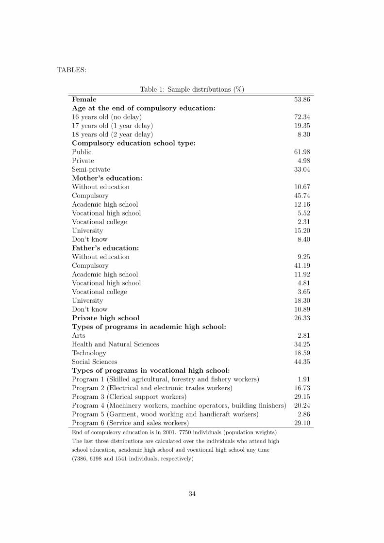
TABLES:

Table 1: Sample distributions (%)Female 53.86Age at the end of compulsory education:16 years old (no delay) 72.3417 years old (1 year delay) 19.3518 years old (2 year delay) 8.30Compulsory education school type:Public 61.98Private 4.98Semi-private 33.04Mother’s education:Without education 10.67Compulsory 45.74Academic high school 12.16Vocational high school 5.52Vocational college 2.31University 15.20Don’t know 8.40Father’s education:Without education 9.25Compulsory 41.19Academic high school 11.92Vocational high school 4.81Vocational college 3.65University 18.30Don’t know 10.89Private high school 26.33Types of programs in academic high school:Arts 2.81Health and Natural Sciences 34.25Technology 18.59Social Sciences 44.35Types of programs in vocational high school:Program 1 (Skilled agricultural, forestry and fishery workers) 1.91Program 2 (Electrical and electronic trades workers) 16.73Program 3 (Clerical support workers) 29.15Program 4 (Machinery workers, machine operators, building finishers) 20.24Program 5 (Garment, wood working and handicraft workers) 2.86Program 6 (Service and sales workers) 29.10End of compulsory education is in 2001. 7750 individuals (population weights)The last three distributions are calculated over the individuals who attend highschool education, academic high school and vocational high school any time(7386, 6198 and 1541 individuals, respectively)

34

Table 2: Age at the end of compulsory educationMale Female

16 years old (no delay) 68.74 75.4217 years old (1 year delay) 21.60 17.4318 years old (2 year delay) 9.66 7.14The end of compulsory education is in 20017750 individuals (population weights)

Table 3: Choice distribution of individuals who start in eachperiod without having completed high school education

School-year AHS VHS1 VHS2 LM Individuals2001/02 79.57 3.66 11.11 5.66 77502002/03 74.72 2.58 11.41 11.29 76272003/04 51.26 2.56 11.49 35.69 30452004/05 27.63 1.06 6.48 64.83 1814

AHS: Academic high school, VHS1: 1-grade vocational high school,VHS2: 2-grade vocational high school, LM: labor marketPopulation weights

Table 4: First decision following compulsory educationAHS VHS LM Total

By gender:Females 83.30 10.74 4.96 100Males 75.22 18.32 6.47 100By age at end of compulsory education:16 years old (no delay) 91.20 6.63 2.17 10017 years old (1 year delay) 54.87 33.16 11.98 10018 years old (2 year delay) 35.81 42.93 21.26 100AHS: Academic high school. VHS: Vocational high school. LM: labor market.7750 individuals (population weights)

35

Table 5: Transition matricesChoice (2002/03)

Choice (2001/02) Academic high school Vocational high school Labor marketAcademic high school 92.25 3.68 4.07Vocational high school 0.46 79.51 20.03Labor market 1.94 5.65 92.41

Choice (2003/04)Choice (2002/03) Academic high school Vocational high school Labor marketAcademic high school 85.45 3.46 11.09Vocational high school 1.49 73.10 25.41Labor market 3.61 3.80 92.59

Choice (2004/05)Choice (2003/04) Academic high school Vocational high school Labor marketAcademic high school 79.83 3.57 16.59Vocational high school 4.15 59.60 36.25Labor market 2.26 2.71 95.03

Choice (t)Choice (t-1) Academic high school Vocational high school Labor marketAcademic high school 89.94 3.63 6.43Vocational high school 1.08 75.96 22.97Labor market 2.69 3.64 93.68Percentage of transitions from origin (choice in t− 1) to destination (choice in t). The first three transitionmatrices are calculated using the total of individuals who start the school-year t without having completed highschool education. The number of individuals is 7627, 3045 and 1814 respectively. The percentages in the last matrixare calculated over total observations in each transition across years (12486 observations). Population weights

Table 6: Completion ratesTotal AHS VHS

Full sample 80.07 78.62 66.85Males 76.27 75.16 62.27Females 83.27 81.30 72.81Graduated over enrolled individuals7750 individuals (population weights)AHS: Academic high schoolVHS: Vocational high school

Table 7: Choice distribution following high school completionUNIV VC VHS AHS LM Total

Academic high school diploma 72.64 18.97 1.52 - 6.87 100Vocational high school diploma - 7.50 7.72 7.04 77.74 1007750 individuals (population weights). UNIV: University, VC: Vocational college,AHS: Academic high school, VHS: Vocational high school, LM: Labor market

36

Table 8: People with a job during the school months (%)School-year AHS VHS1 VHS2 LM2001/02 8.13 27.58 18.78 89.782002/03 9.18 35.27 25.60 91.772003/04 18.95 33.53 38.59 96.622004/05 43.02 23.06 41.87 96.77

School months: October to May (both included)7750 individuals (population weights)AHS: Academic high school, VHS1: 1-grade vocationalhigh school, VHS2: 2-grade vocational high schoolLM: labor market

Table 9: Completion rates following a high school diplomaAcademic high school Vocational high schoolMales Females Males Females

University 59.37 67.33 - -VC 77.67 84.81 67.82 68.53VHS 67.34 51.56 75.90 79.89AHS - - 53.57 58.31Source: ETEFIL samples of academic and vocational high schoolgraduates in 2000/2001 (population weights)AHS: Academic high school, VHS: Vocational high schoolVC: Vocational college

37

Table 10: Life-cycle premiumAcademic diploma Vocational diploma

UNIV VC VHS LM VC AHS VHS LMRegion:Northwest 1.62 1.39 1.42 1.42 1.39 1.43 1.42 1.40Northeast 1.56 1.42 1.34 1.27 1.43 1.33 1.37 1.36Centre 1.81 1.54 1.42 1.52 1.48 1.46 1.36 1.34East 1.61 1.44 1.35 1.39 1.41 1.38 1.33 1.31South 1.75 1.50 1.44 1.50 1.46 1.47 1.39 1.38Gender:Male 1.54 1.37 1.33 1.34 1.36 1.34 1.32 1.31Female 1.88 1.60 1.50 1.54 1.56 1.52 1.45 1.44

Total 1.67 1.46 1.39 1.41 1.43 1.41 1.37 1.35Present discounted value of life-cycle earnings corresponding to compulsoryschooling equal to one. Source: Spanish Wage Structure Survey 2002UNIV: university, VC: Vocational college, VHS: Vocational high schoolAHS: Academic high school, LM: Labor marketNorthwest: Galicia, Asturias, Cantabria. Northeast: Pais Vasco, La Rioja,Navarra, Aragon. Centre: Castilla-Leon, Castilla-La Mancha, Extremadura,Madrid. East: Cataluña, Valencia, Islas Baleares. South: Andalucia, Murcia,Islas Canarias, Ceuta y Melilla

Table 11: Estimates of the utility function parameters

Number of accumulated passed grades in AHS 56,986.68 (1,498.07)Number of accumulated passed grades in VHS 82,825.56 (1,211.50)Reenrollment cost in AHS after a period working -14,790.45 (1,054.20)Reenrollment cost in VHS after a period working -22,650.61 (979.67)

Constants:AHS (µAHS) -55,140.28 (783.54)VHS type 1 (µV HS1 ) -83,202.01 (1,326.87)VHS type 2 (µV HS2 ) -51,318.17 (805.38)

Type 1 probability (π1) 0.61 (0.02)M = 2 and β = 0.97. Estimates expressed in monetary equivalent units (euros of 2001)Standard errors are in parentheses. They are calculated using numerical second derivativesLikelihood = -15,678.39. AHS: Academic high school, VHS: Vocational high school

38

Table 12: Estimates of the transition probability parameters1. Probability of passing a complete grade in academic high school (cAHSt = 1)

School-year2001/02 2002/03 2003/04

Female 0.26 (0.07) 0.28 (0.07) 0.12 (0.11)Finished compulsory schooling with delay -1.51 (0.07) -1.24 (0.08) -0.39 (0.12)nAHS - - 0.10 (0.09) 0.48 (0.23)Intercept 1.65 (0.05) 1.25 (0.10) 0.19 (0.24)Individuals enrolled in the academic track 6171 5727 1577

2. Probability of passing a complete grade in vocational high school (cV HSt = 1)School-year

2001/02 2002/03 2003/04Female -0.20 (0.12) 0.34 (0.16) 0.64 (0.25)Finished compulsory schooling with delay -0.41 (0.14) -0.65 (0.16) -0.28 (0.24)nV HS - - 0.90 (0.15) 0.96 (0.24)Intercept 0.97 (0.13) 1.07 (0.17) 0.37 (0.23)Individuals enrolled in the vocational track 1171 1079 402Estimates obtained using a logit specification for both probabilities. The dependent variable takes value onein the school-year t if the individual passed the grade. Standard errors are in parenthesesnAHS and nV HS are the number of accumulated passed grades in academic and vocational high school,respectively. Finished compulsory schooling with delay is a dummy variable equal to one if the individualcompleted compulsory schooling with more than sixteen years old

Table 13: Predicted statistics (%)Actual Predicted

High school graduates 76.00 79.66Vocational graduates among high school graduates 17.31 19.03Females among high school graduates 55.21 55.12Females among academic high school graduates 57.31 58.83Females among vocational high school graduates 45.20 39.32Individuals who attend academic high school 79.93 82.72Individuals who attend vocational high school 19.68 18.22Individuals who never attend post-compulsory education 5.08 4.45Individuals who switch between academic and vocational HS 4.69 5.39Predicted statistics obtained by simulating schooling histories for 7750 individuals using theparameter estimates from Tables 11 and 12

39

Table 14: Choice distribution of individuals who start in each period withouthaving completed high school education

AHS VHS LMSchool-year Actual Predicted Actual Predicted Actual Predicted2001/02 79.57 82.00 14.77 12.45 5.66 5.552002/03 74.72 75.27 13.99 15.28 11.29 9.462003/04 51.26 54.49 13.05 17.79 35.69 27.722004/05 27.63 16.31 7.55 4.06 64.83 79.63

AHS: Academic high school, VHS: Vocational high school, LM: labor marketPredicted statistics obtained by simulating schooling histories for 7750 individuals using theparameter estimates from Tables 11 and 12

Table 15: Predicted transition matrixChoice (t)

Choice (t-1) Acad. high school Voc. high school Labor marketAcad. high school 86.46 (89.94) 4.55 (3.63) 8.98 (6.43)Voc. high school 1.07 (1.08) 87.33 (75.96) 11.60 (22.97)Labor market 3.42 (2.69) 3.27 (3.64) 93.31 (93.68)Percentage of transitions from origin (choice in t− 1) to destination (choice in t).The percentages are calculated over total observations in each transition across years.They are based on a simulation of schooling histories for 7750 individuals using theparameter estimates from Tables 11 and 12. The actual values are shown in parentheses

Table 16: Predicted completion rates (%)Total AHS VHS

Actual Predicted Actual Predicted Actual PredictedFull sample 80.07 83.38 78.62 77.98 66.85 83.22Males 76.27 80.39 75.16 74.22 62.27 81.95Females 83.27 85.98 81.30 80.84 72.81 85.24Graduated over enrolled individuals. AHS: Academic high school, VHS: Vocational highschool. Percentages obtained by simulating schooling histories for 7750 individuals usingthe parameter estimates from Tables 11 and 12

Table 17: Predicted choice distribution following high school completionUNIV VC VHS AHS LM Total

Academic high school diploma 100 0 0 - 0 100Vocational high school diploma - 79.49 0 20.51 0 100Percentages obtained by simulating schooling histories for 7750 individuals using theparameter estimates from Tables 11 and 12. UNIV: University, VC: Vocational college,AHS: Academic high school, VHS: Vocational high school, LM: Labor market

40

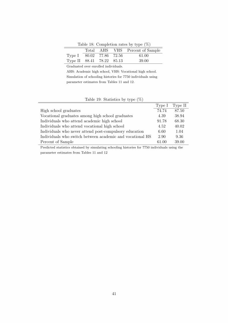
Table 18: Completion rates by type (%)Total AHS VHS Percent of Sample

Type I 80.02 77.86 72.56 61.00Type II 88.41 78.22 85.13 39.00Graduated over enrolled individuals.AHS: Academic high school, VHS: Vocational high school.Simulation of schooling histories for 7750 individuals usingparameter estimates from Tables 11 and 12.

Table 19: Statistics by type (%)Type I Type II

High school graduates 74.74 87.50Vocational graduates among high school graduates 4.39 38.94Individuals who attend academic high school 91.78 68.30Individuals who attend vocational high school 4.52 40.02Individuals who never attend post-compulsory education 6.60 1.04Individuals who switch between academic and vocational HS 2.90 9.36Percent of Sample 61.00 39.00Predicted statistics obtained by simulating schooling histories for 7750 individuals using theparameter estimates from Tables 11 and 12

41

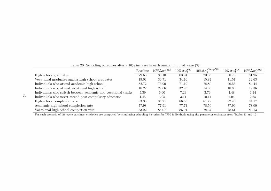
Table 20: Schooling outcomes after a 10% increase in each annual imputed wage (%)Baseline 10%∆wV HSt 10%∆wV Ct 10%∆wCompDipt 10%∆wUNt 10%∆wAHSt

High school graduates 79.66 83.10 83.94 73.50 80.75 81.95Vocational graduates among high school graduates 19.03 30.71 34.10 15.84 11.57 19.63Individuals who attend academic high school 82.72 73.90 71.19 78.80 90.56 84.44Individuals who attend vocational high school 18.22 29.66 32.93 14.85 10.88 19.36Individuals who switch between academic and vocational tracks 5.39 6.60 7.23 3.79 4.48 6.44Individuals who never attend post-compulsory education 4.45 3.05 3.11 10.14 2.04 2.65High school completion rate 83.38 85.71 86.63 81.79 82.43 84.17Academic high school completion rate 77.98 77.91 77.71 78.50 77.99 78.00Vocational high school completion rate 83.22 86.07 86.91 78.37 78.61 83.13For each scenario of life-cycle earnings, statistics are computed by simulating schooling histories for 7750 individuals using the parameter estimates from Tables 11 and 12

42

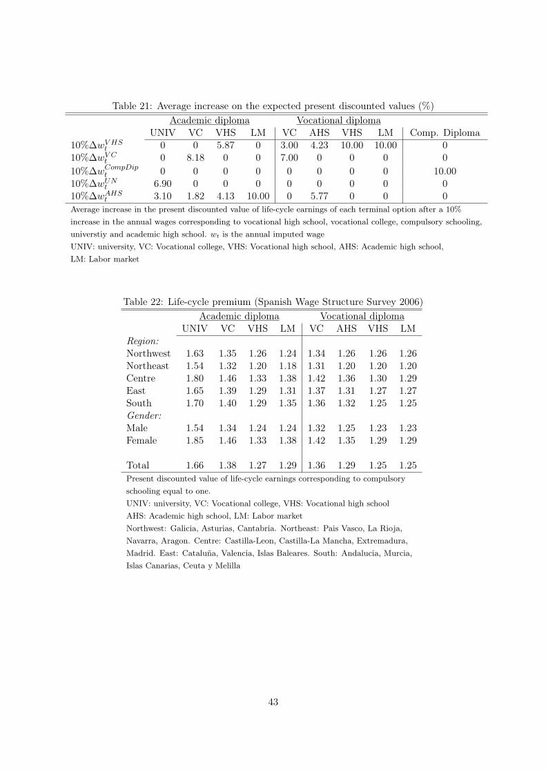
Table 21: Average increase on the expected present discounted values (%)Academic diploma Vocational diploma

UNIV VC VHS LM VC AHS VHS LM Comp. Diploma10%∆wV HSt 0 0 5.87 0 3.00 4.23 10.00 10.00 010%∆wV Ct 0 8.18 0 0 7.00 0 0 0 010%∆wCompDipt 0 0 0 0 0 0 0 0 10.0010%∆wUNt 6.90 0 0 0 0 0 0 0 010%∆wAHSt 3.10 1.82 4.13 10.00 0 5.77 0 0 0Average increase in the present discounted value of life-cycle earnings of each terminal option after a 10%increase in the annual wages corresponding to vocational high school, vocational college, compulsory schooling,universtiy and academic high school. wt is the annual imputed wageUNIV: university, VC: Vocational college, VHS: Vocational high school, AHS: Academic high school,LM: Labor market

Table 22: Life-cycle premium (Spanish Wage Structure Survey 2006)Academic diploma Vocational diploma

UNIV VC VHS LM VC AHS VHS LMRegion:Northwest 1.63 1.35 1.26 1.24 1.34 1.26 1.26 1.26Northeast 1.54 1.32 1.20 1.18 1.31 1.20 1.20 1.20Centre 1.80 1.46 1.33 1.38 1.42 1.36 1.30 1.29East 1.65 1.39 1.29 1.31 1.37 1.31 1.27 1.27South 1.70 1.40 1.29 1.35 1.36 1.32 1.25 1.25Gender:Male 1.54 1.34 1.24 1.24 1.32 1.25 1.23 1.23Female 1.85 1.46 1.33 1.38 1.42 1.35 1.29 1.29

Total 1.66 1.38 1.27 1.29 1.36 1.29 1.25 1.25Present discounted value of life-cycle earnings corresponding to compulsoryschooling equal to one.UNIV: university, VC: Vocational college, VHS: Vocational high schoolAHS: Academic high school, LM: Labor marketNorthwest: Galicia, Asturias, Cantabria. Northeast: Pais Vasco, La Rioja,Navarra, Aragon. Centre: Castilla-Leon, Castilla-La Mancha, Extremadura,Madrid. East: Cataluña, Valencia, Islas Baleares. South: Andalucia, Murcia,Islas Canarias, Ceuta y Melilla

43

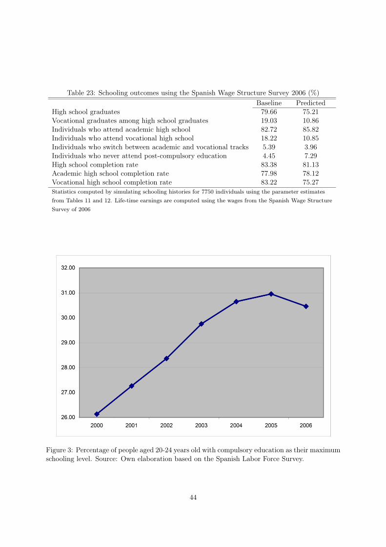
Table 23: Schooling outcomes using the Spanish Wage Structure Survey 2006 (%)Baseline Predicted

High school graduates 79.66 75.21Vocational graduates among high school graduates 19.03 10.86Individuals who attend academic high school 82.72 85.82Individuals who attend vocational high school 18.22 10.85Individuals who switch between academic and vocational tracks 5.39 3.96Individuals who never attend post-compulsory education 4.45 7.29High school completion rate 83.38 81.13Academic high school completion rate 77.98 78.12Vocational high school completion rate 83.22 75.27Statistics computed by simulating schooling histories for 7750 individuals using the parameter estimatesfrom Tables 11 and 12. Life-time earnings are computed using the wages from the Spanish Wage StructureSurvey of 2006

Figure 3: Percentage of people aged 20-24 years old with compulsory education as their maximumschooling level. Source: Own elaboration based on the Spanish Labor Force Survey.

44

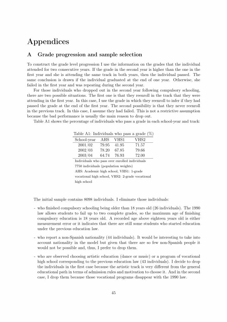
Appendices

A Grade progression and sample selection

To construct the grade level progression I use the information on the grades that the individualattended for two consecutive years. If the grade in the second year is higher than the one in thefirst year and she is attending the same track in both years, then the individual passed. Thesame conclusion is drawn if the individual graduated at the end of one year. Otherwise, shefailed in the first year and was repeating during the second year.

For those individuals who dropped out in the second year following compulsory schooling,there are two possible situations. The first one is that they reenroll in the track that they wereattending in the first year. In this case, I use the grade in which they reenroll to infer if they hadpassed the grade at the end of the first year. The second possibility is that they never reenrollin the previous track. In this case, I assume they had failed. This is not a restrictive assumptionbecause the bad performance is usually the main reason to drop out.

Table A1 shows the percentage of individuals who pass a grade in each school-year and track:

Table A1: Individuals who pass a grade (%)School-year AHS VHS1 VHS22001/02 79.95 41.95 71.572002/03 78.20 67.85 79.662003/04 64.74 76.93 72.00

Individuals who pass over enrolled individuals7750 individuals (population weights)AHS: Academic high school, VHS1: 1-gradevocational high school, VHS2: 2-grade vocationalhigh school

The initial sample contains 8098 individuals. I eliminate those individuals:

- who finished compulsory schooling being older than 18 years old (26 individuals). The 1990law allows students to fail up to two complete grades, so the maximum age of finishingcompulsory education is 18 years old. A recorded age above eighteen years old is eithermeasurement error or it indicates that there are still some students who started educationunder the previous education law.

- who report a non-Spanish nationality (44 individuals). It would be interesting to take intoaccount nationality in the model but given that there are so few non-Spanish people itwould not be possible and, thus, I prefer to drop them.

- who are observed choosing artistic education (dance or music) or a program of vocationalhigh school corresponding to the previous education law (43 individuals). I decide to dropthe individuals in the first case because the artistic track is very different from the generaleducational path in terms of admission rules and motivation to choose it. And in the secondcase, I drop them because those vocational programs disappear with the 1990 law.

45

- who have inconsistent responses over the survey (40 individuals). For example, they areobserved attending university but previously they do not report an academic high schooldiploma.

In total I eliminate 153 individuals and the final sample size is 7945. The eliminated individualsonly represent 1.89% of the initial sample and dropping them does not generate any differencebetween the initial and the final samples.

46

B Reduced form estimations

Table B1: Probability of choosing academic high school each yeart = 1 t = 2 t = 3 t = 4

Variable Coefficient Std. Error Coefficient Std. Error Coefficient Std. Error Coefficient Std. ErrornAHS - - 5.84∗∗ (0.25) 4.72∗∗ (0.18) 3.41∗∗ (0.23)dt−1 = LM - - -2.92∗∗ (0.35) -1.43∗∗ (0.24) -2.65∗∗ (0.24)Private school in AHS 0.02 (0.12) -0.39∗∗ (0.14) 0.40∗ (0.19) 0.65∗ (0.28)Female 0.59∗∗ (0.07) 0.52∗∗ (0.10) 0.41∗ (0.16) 0.21 (0.18)+ 16 years old -2.40∗∗ (0.07) -1.52∗∗ (0.10) -0.77∗∗ (0.16) -0.47∗ (0.19)School type in compulsory education (ref: public school):Private 1.18∗∗ (0.28) 0.44 (0.31) -0.39 (0.66) 0.15 (0.49)Semi-private 0.36∗∗ (0.10) 0.28∗ (0.11) 0.13 (0.18) -0.24 (0.21)Mother education (ref: compulsory diploma):Without education -0.44∗∗ (0.13) -0.33† (0.17) -0.49† (0.30) -0.01 (0.39)AHS 0.63∗∗ (0.13) 0.63∗∗ (0.18) 0.22 (0.30) 0.50 (0.30)VHS 0.42∗ (0.17) 0.21 (0.21) -0.14 (0.37) 0.01 (0.48)VC 0.34 (0.28) 0.61 (0.39) 0.70 (0.62) 0.10 (0.53)UNIV 1.04∗∗ (0.19) 0.73∗∗ (0.21) 0.41 (0.39) 0.48 (0.39)Don’t know -0.05 (0.17) -0.31 (0.24) -0.38 (0.46) -0.18 (0.45)Father education (ref: compulsory diploma):Without education 0.10 (0.14) 0.37∗ (0.18) -0.29 (0.32) 0.21 (0.40)AHS 0.55∗∗ (0.12) 0.37∗ (0.17) 0.10 (0.27) 0.16 (0.32)VHS 0.02 (0.16) 0.17 (0.24) 0.57 (0.36) 1.18† (0.72)VC 0.64∗∗ (0.21) 0.50† (0.27) 0.59 (0.49) -0.34 (0.42)UNIV 1.19∗∗ (0.16) 0.89∗∗ (0.20) 1.02∗∗ (0.32) 0.14 (0.35)Don’t know -0.32∗ (0.16) 0.15 (0.21) 0.11 (0.44) 0.24 (0.41)Regions (ref: south):Northwest -0.02 (0.11) -0.10 (0.17) -0.14 (0.26) -0.24 (0.28)Northeast -0.23∗ (0.11) -0.78∗∗ (0.17) -0.09 (0.27) -0.36 (0.33)Center 0.22∗ (0.10) 0.17 (0.14) 0.50∗ (0.24) 0.28 (0.24)East -0.76∗∗ (0.10) -0.60∗∗ (0.13) -0.16 (0.22) -0.01 (0.25)Intercept 1.83∗∗ (0.10) -0.29∗ (0.13) -2.25∗∗ (0.26) -2.10∗∗ (0.31)Significance levels: † : 10% ∗ : 5% ∗∗ : 1%. Robust standard errors. 7750 individualsLogit specification

47

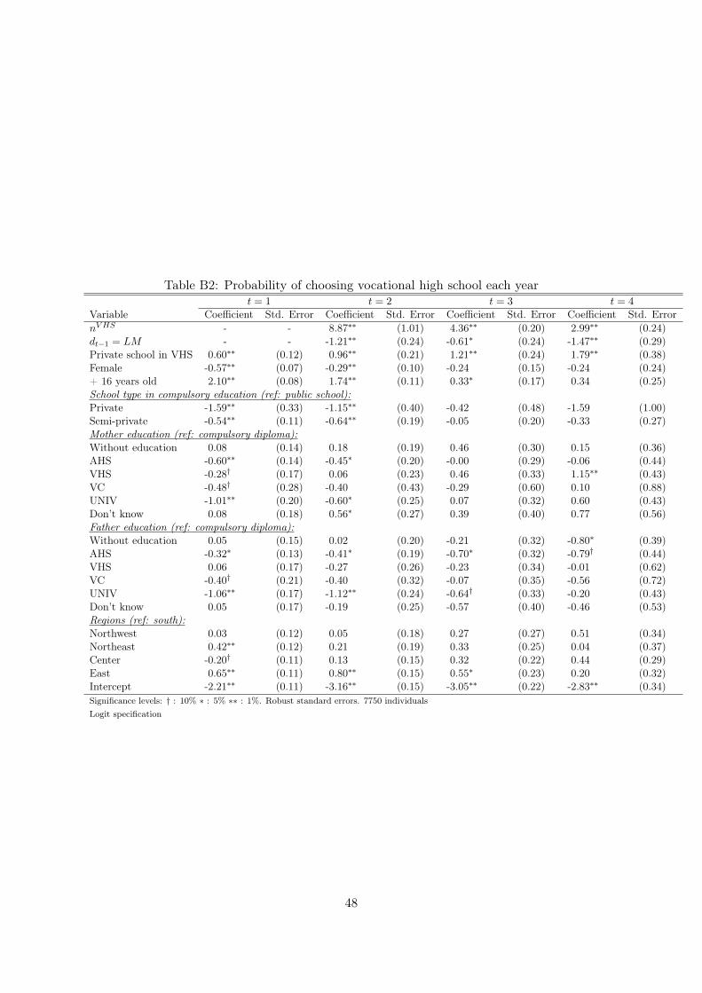
Table B2: Probability of choosing vocational high school each yeart = 1 t = 2 t = 3 t = 4

Variable Coefficient Std. Error Coefficient Std. Error Coefficient Std. Error Coefficient Std. ErrornV HS - - 8.87∗∗ (1.01) 4.36∗∗ (0.20) 2.99∗∗ (0.24)dt−1 = LM - - -1.21∗∗ (0.24) -0.61∗ (0.24) -1.47∗∗ (0.29)Private school in VHS 0.60∗∗ (0.12) 0.96∗∗ (0.21) 1.21∗∗ (0.24) 1.79∗∗ (0.38)Female -0.57∗∗ (0.07) -0.29∗∗ (0.10) -0.24 (0.15) -0.24 (0.24)+ 16 years old 2.10∗∗ (0.08) 1.74∗∗ (0.11) 0.33∗ (0.17) 0.34 (0.25)School type in compulsory education (ref: public school):Private -1.59∗∗ (0.33) -1.15∗∗ (0.40) -0.42 (0.48) -1.59 (1.00)Semi-private -0.54∗∗ (0.11) -0.64∗∗ (0.19) -0.05 (0.20) -0.33 (0.27)Mother education (ref: compulsory diploma):Without education 0.08 (0.14) 0.18 (0.19) 0.46 (0.30) 0.15 (0.36)AHS -0.60∗∗ (0.14) -0.45∗ (0.20) -0.00 (0.29) -0.06 (0.44)VHS -0.28† (0.17) 0.06 (0.23) 0.46 (0.33) 1.15∗∗ (0.43)VC -0.48† (0.28) -0.40 (0.43) -0.29 (0.60) 0.10 (0.88)UNIV -1.01∗∗ (0.20) -0.60∗ (0.25) 0.07 (0.32) 0.60 (0.43)Don’t know 0.08 (0.18) 0.56∗ (0.27) 0.39 (0.40) 0.77 (0.56)Father education (ref: compulsory diploma):Without education 0.05 (0.15) 0.02 (0.20) -0.21 (0.32) -0.80∗ (0.39)AHS -0.32∗ (0.13) -0.41∗ (0.19) -0.70∗ (0.32) -0.79† (0.44)VHS 0.06 (0.17) -0.27 (0.26) -0.23 (0.34) -0.01 (0.62)VC -0.40† (0.21) -0.40 (0.32) -0.07 (0.35) -0.56 (0.72)UNIV -1.06∗∗ (0.17) -1.12∗∗ (0.24) -0.64† (0.33) -0.20 (0.43)Don’t know 0.05 (0.17) -0.19 (0.25) -0.57 (0.40) -0.46 (0.53)Regions (ref: south):Northwest 0.03 (0.12) 0.05 (0.18) 0.27 (0.27) 0.51 (0.34)Northeast 0.42∗∗ (0.12) 0.21 (0.19) 0.33 (0.25) 0.04 (0.37)Center -0.20† (0.11) 0.13 (0.15) 0.32 (0.22) 0.44 (0.29)East 0.65∗∗ (0.11) 0.80∗∗ (0.15) 0.55∗ (0.23) 0.20 (0.32)Intercept -2.21∗∗ (0.11) -3.16∗∗ (0.15) -3.05∗∗ (0.22) -2.83∗∗ (0.34)Significance levels: † : 10% ∗ : 5% ∗∗ : 1%. Robust standard errors. 7750 individualsLogit specification

48

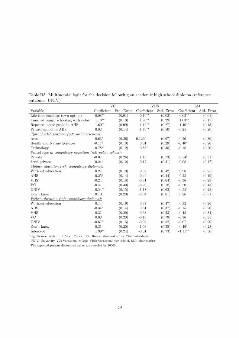
Table B3: Multinomial logit for the decision following an academic high school diploma (referenceoutcome: UNIV)

VC VHS LMVariable Coefficient Std. Error Coefficient Std. Error Coefficient Std. ErrorLife-time earnings (own option) -0.08∗∗ (0.01) -0.10∗∗ (0.02) -0.03∗∗ (0.01)Finished comp. schooling with delay 1.18∗∗ (0.13) 1.90∗∗ (0.29) 1.03∗∗ (0.17)Repeated some grade in AHS 1.60∗∗ (0.09) 1.19∗∗ (0.27) 1.46∗∗ (0.13)Private school in AHS 0.02 (0.14) -1.76∗∗ (0.50) -0.25 (0.20)Type of AHS program (ref: social sciences):Arts 0.63∗ (0.26) 0.1260 (0.67) 0.26 (0.36)Health and Nature Sciences -0.17† (0.10) 0.01 (0.29) -0.40∗ (0.20)Technology 0.78∗∗ (0.12) 0.85∗ (0.35) -0.18 (0.20)School type in compulsory education (ref: public school):Private -0.07 (0.26) 1.10 (0.73) 0.54† (0.31)Semi-private -0.24∗ (0.12) 0.12 (0.31) -0.08 (0.17)Mother education (ref: compulsory diploma):Without education 0.24 (0.19) 0.66 (0.42) 0.28 (0.25)AHS -0.25† (0.14) -0.49 (0.44) 0.25 (0.19)VHS -0.24 (0.18) -0.81 (0.64) -0.36 (0.29)VC -0.41 (0.30) -0.20 (0.78) -0.20 (0.43)UNIV -0.54∗∗ (0.15) -1.18† (0.63) -0.55∗ (0.23)Don’t know 0.10 (0.23) -0.04 (0.61) 0.26 (0.31)Father education (ref: compulsory diploma):Without education 0.14 (0.19) 0.37 (0.47) 0.32 (0.26)AHS -0.34∗ (0.14) 0.61† (0.37) -0.15 (0.20)VHS -0.31 (0.20) 0.63 (0.53) -0.45 (0.34)VC 0.03 (0.20) -0.10 (0.79) -0.36 (0.35)UNIV -0.67∗∗ (0.15) -0.02 (0.52) -0.07 (0.20)Don’t know 0.31 (0.20) 1.03† (0.55) 0.49† (0.28)Intercept 1.99∗∗ (0.24) -0.31 (0.73) -1.11∗∗ (0.36)Significance levels: † : 10% ∗ : 5% ∗∗ : 1%. Robust standard errors. 7750 individuals.UNIV: University, VC: Vocational college, VHS: Vocational high school, LM: labor market.The expected present discounted values are rescaled by 10000.

49

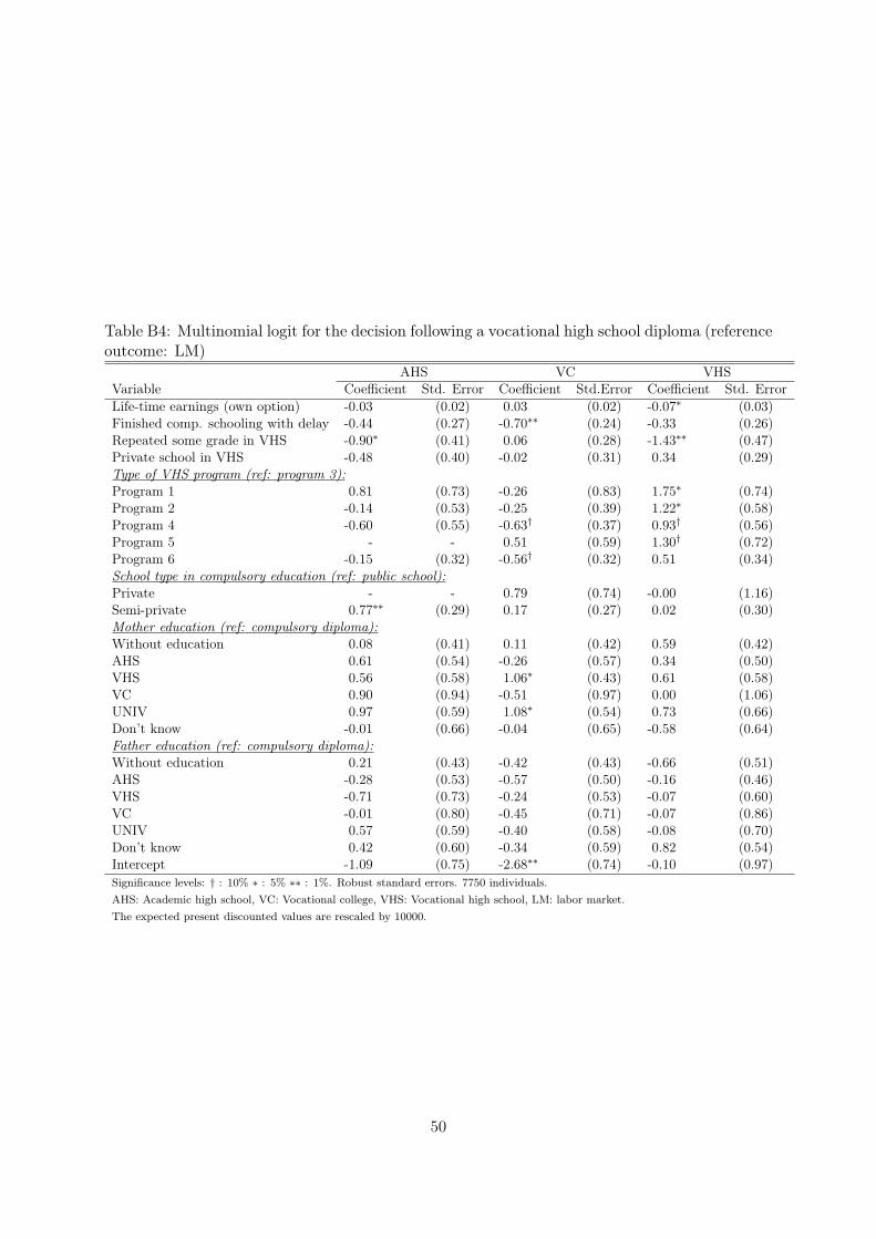
Table B4: Multinomial logit for the decision following a vocational high school diploma (referenceoutcome: LM)

AHS VC VHSVariable Coefficient Std. Error Coefficient Std.Error Coefficient Std. ErrorLife-time earnings (own option) -0.03 (0.02) 0.03 (0.02) -0.07∗ (0.03)Finished comp. schooling with delay -0.44 (0.27) -0.70∗∗ (0.24) -0.33 (0.26)Repeated some grade in VHS -0.90∗ (0.41) 0.06 (0.28) -1.43∗∗ (0.47)Private school in VHS -0.48 (0.40) -0.02 (0.31) 0.34 (0.29)Type of VHS program (ref: program 3):Program 1 0.81 (0.73) -0.26 (0.83) 1.75∗ (0.74)Program 2 -0.14 (0.53) -0.25 (0.39) 1.22∗ (0.58)Program 4 -0.60 (0.55) -0.63† (0.37) 0.93† (0.56)Program 5 - - 0.51 (0.59) 1.30† (0.72)Program 6 -0.15 (0.32) -0.56† (0.32) 0.51 (0.34)School type in compulsory education (ref: public school):Private - - 0.79 (0.74) -0.00 (1.16)Semi-private 0.77∗∗ (0.29) 0.17 (0.27) 0.02 (0.30)Mother education (ref: compulsory diploma):Without education 0.08 (0.41) 0.11 (0.42) 0.59 (0.42)AHS 0.61 (0.54) -0.26 (0.57) 0.34 (0.50)VHS 0.56 (0.58) 1.06∗ (0.43) 0.61 (0.58)VC 0.90 (0.94) -0.51 (0.97) 0.00 (1.06)UNIV 0.97 (0.59) 1.08∗ (0.54) 0.73 (0.66)Don’t know -0.01 (0.66) -0.04 (0.65) -0.58 (0.64)Father education (ref: compulsory diploma):Without education 0.21 (0.43) -0.42 (0.43) -0.66 (0.51)AHS -0.28 (0.53) -0.57 (0.50) -0.16 (0.46)VHS -0.71 (0.73) -0.24 (0.53) -0.07 (0.60)VC -0.01 (0.80) -0.45 (0.71) -0.07 (0.86)UNIV 0.57 (0.59) -0.40 (0.58) -0.08 (0.70)Don’t know 0.42 (0.60) -0.34 (0.59) 0.82 (0.54)Intercept -1.09 (0.75) -2.68∗∗ (0.74) -0.10 (0.97)Significance levels: † : 10% ∗ : 5% ∗∗ : 1%. Robust standard errors. 7750 individuals.AHS: Academic high school, VC: Vocational college, VHS: Vocational high school, LM: labor market.The expected present discounted values are rescaled by 10000.

50