Demand Estimation Under IncompleteProduct Availability∗

Christopher T. ConlonJulie Holland Mortimer

June 30, 2007

Abstract

Stockout events are a common feature of retail markets. When stockouts changethe set of available products, observed sales provide a biased estimate of demand. Ifa product sells out, actual demand may be greater than observed sales, leading to anegative bias in demand estimates. At the same time, sales of substitute products mayincrease. Such events generate variation in choice sets, which is an important sourceof identification in the IO literature. In this paper, we develop a simple procedurethat allows for variation in choice sets within a “market” over time using panel data.This allows for consistent estimation of demand even when stockouts imply that theset of available options varies endogenously. We estimate demand in the presence ofstockouts using data from vending machines, which track sales and product availability.When the corrected estimates are compared with naive estimates, the size of the biasdue to ignoring stockouts is shown to be large.

∗We thank Susan Athey, Steve Berry, Uli Doraszelski, Phil Haile, Ken Hendricks, Phillip Leslie, and ArielPakes for helpful discussions and comments. Financial support for this research was generously providedthrough NSF grant SES-0617896.

1 Introduction

Retail and service markets account for 30% of GDP and 48% of employment in the US,yet most economic models assume that retail settings are unimportant for understandingconsumer demand and firms’ decisions. Specifically, most methods of demand analysis rely onthe assumption that all products are available to all consumers. While many industries, suchas automobiles and computer chips, have been successfully analyzed under this assumption(Berry, Levinsohn, and Pakes 1995), research into many retail markets suggests that retailsettings are characterized by important deviations from this model. Specifically, “stock-outs” of products, or periods where products are unavailable are common in many settings.Furthermore, both producers and consumers identify product availability as an importantconsideration in these markets. When the goods in question are perishable or seasonal, orgenerally lack inter-temporal substitutability, management of inventory is not an ancillaryconcern; it is the primary problem that firms address. When stockouts change the set ofavailable products, observed sales provide a biased estimate of demand for two reasons. Thefirst source of bias is the censoring of demand estimates. If a product sells out, the actualdemand for a product may be greater than the observed sales, leading to a negative biasin demand estimates. At the same time, during periods of reduced availability of otherproducts, sales of available products may increase. This forced substitution overstates thetrue demand for these goods.

The current class of discrete choice models prevalent in the IO literature is able to addressvariation in the choice sets facing consumers across markets. In fact, variation in choice setsacross markets is an important source of identification in these models. In this paper, wedevelop a simple procedure that allows for variation in choice sets within a “market” overtime using panel data. This allows for consistent estimation of demand even when stockoutsimply that the set of available options varies endogenously.

If the choice set facing the consumer were observed when each choice was made, correctingdemand estimates would be simple. However, in many real world applications inventories areonly observed periodically. This presents an additional challenge for estimation, because theregime under which choices took place must be estimated in addition to parameters. Thank-fully, this is a well understood missing data problem and the EM algorithm of Dempster,Laird, and Rubin (1977) applies.

The dataset that we use tracks the sales of snack foods in vending machines locatedon the campus of Arizona State University (ASU). Wireless observations of the sales andproduct availability, along with numerous and repeated observations of stock-outs, make thisdataset well-adapted to the analysis of product availability.

When the corrected estimates are compared with the naive estimates, the size of the biasis shown to be large, and the welfare implications of stockouts would be substantially mis-measured with naive estimates. This paper focuses only on the static analysis of demand inthe presence of reduced product availability. It does not consider either dynamic interactionsor the problem of the retailer.

1

2 Relationship to Literature

The differentiated products literature in IO has been primarily focused on two methodolog-ical problems. The first is the endogeneity of prices (Berry 1994), and the second is thedetermination of accurate substitution patterns. Berry, Levinsohn, and Pakes (1995) useunobserved product quality and unobserved tastes for product characteristics to more flexi-bly (and accurately) predict substitution patterns. The fundamental source of identificationin these models comes through variation in choice sets across markets (typically through theprice). Nevo (2001) uses a similar model to study a retail environment in his analysis ofthe market for Ready to Eat (RTE) Cereal. Further work (Petrin 2002, Berry, Levinsohn,and Pakes 2004) has focused on using interactions of consumer observables and productcharacteristics to better estimate substitution patterns. Berry, Levinsohn, and Pakes (2004)extend this idea even further and use second choice data from surveys in which consumersare asked which product they would have purchased if their original choice was unavailable.This paper’s approach is a bit different because consumer level stated second choice dataare unobserved, and substitution patterns are instead inferred from revealed substitutionby exploiting short-run variations in the set of available choices. Recently, there have beenseveral attempts made to present a fully bayesian model of discrete choice consumer demandamong them Musalem, Bradlow, and Raju (2006). While this paper uses a common Bayesiantechnique to address missing data, it is not a fully Bayesian model.

There is also a substantial literature in IO on the dynamics of price and inventory.Previous studies have looked at the effect of coupons and sales on future demand in terms of“consumer inventories” (durable goods) (Nevo and Hendel 2007b, Nevo and Hendel 2007a,Nevo and Wolfram 2002). And other studies have looked at the dynamic interaction betweenretailer inventories (and the cost of holding them) and the markups extracted by the retailer(Aguirregabiria 1999). While retailer inventories are explicitly modeled in the example weexamine, these sorts of dynamics are not an issue because the retailer does not have theability to dynamically alter the control (price or product mix). In fact, vending is a usefulindustry to study product availability precisely because we need not worry about these otherdynamic effects.

Stock-outs are frequently analyzed in the context of optimal inventory policies in oper-ations research. In fact, an empirical analysis of stock-out based substitution has been ad-dressed using vending data before by Anupindi, Dada, and Gupta (1998) (henceforth ADG).ADG use an eight-product soft-drink machine and observe the inventory at the beginningof each day. The authors assume that products are sold at a constant Poisson distributedrate (cans per hour). The sales rates of the products are treated as independent from oneanother, and eight Poisson parameters are estimated. When a stock-out occurs, a new setof parameters is estimated with the restriction that the new set of parameters are at leastas great as the original parameters. This means that each choice set requires its own setof parameters (and observed sales). If a Poisson rate was not fitted for a particular choiceset, then only bounds can be inferred from the model. Estimating too many parameters isavoided by assuming that consumers leave the machine if their first two choices are unavail-able. ADG did not observe the stock-out time and used E-M techniques (Dempster, Laird,and Rubin 1977) to estimate the Poisson model in the presence of missing choice set data.

2

This paper aims to connect these two literatures, by using modern differentiated productestimation techniques to obtain accurate estimates of substitution patterns while reducingthe parameter space and applying missing data techniques to correct these estimates forstockout based substitution.

2.1 Inventory Systems

When talking about inventory systems we use the standard dichotomy established by Hadleyand Whitman (1963). The first type of inventory system is called a “perpetual” data system.In this system, product availability is known and recorded when each purchase is made. Thusfor every purchase, the retailer knows exactly how many units of each product are available.This system is also known as “real-time” inventory.1

The other type of inventory system is known as a “periodic” inventory system. In thissystem, inventory is measured only at the beginning of each period. After the initial measure-ment, sales take place, but inventory is not measured again until the next period. Periodicinventory systems are problematic in analyses of stock-outs, because inventory (and thusthe consumer’s choice set) is not recorded with each transaction. While real-time inven-tory systems are becoming more common in retailing environments thanks to innovations ininformation technology, most retailers still do not have access to real-time inventory data.However, periodic inventory systems can be used to approximate perpetual data. As the sizeof the sampling period becomes sufficiently small, periodic data approaches perpetual data.In the limit where the inventory is sampled between each transaction, this is equivalent tohaving real-time data. These two points become very important in the estimation section.

Sampling inventory more frequently helps to mitigate limitations of the periodic inventorysystem. However, the methodological goal of this paper is to provide consistent estimates ofdemand not only for perpetual inventory systems but for periodic ones as well.

3 Model

A typical starting point in discrete choice models is to begin by writing down a consumer’sutility function. However, instead of doing that we consider what the observed data looklike, and try to write down an expression for the likelihood. Assume that the observeddata are broken up into time periods t = 1, 2, . . . , T and that products are denoted by thesubscript j = 1, 2, . . . , J . For each product, denote yjt as the quantity sold of the product jin period t. It is important to note that the precise order of sales may be unobserved, withonly aggregate data available for each period t.

We assume that in each period t, and there are Mt potential consumers.2 This is a typicalassumption in the differentiated products literature (Mt is often based on census data suchas in Berry, Levinsohn, and Pakes (1995) or Nevo (2001)). In this section we assume thatthe set of available products at is constant within a period. We relax this assumption in thenext section.

1Note that if sales are recorded in the order they happen, this would be sufficient to construct an almost“perpetual” inventory system (assuming consumers do not hold goods for long before purchasing an item).

2This assumption can be relaxed later.

3

Assumption 1. (Discrete Choice) Each of the Mt consumers in period t must either choose

some product j ∈ at or the outside good j = 0.

Assumption 2. (Independence of Consumers) Each consumer’s preferences are independent

of other consumer’s preferences (and choices) and each set of preferences is the realization

of an i.i.d. draw from some stable population distribution (perhaps conditional on some xt)

Assumption 1 states that each of the Mt consumers face a choice: they may buy exactlyone product j in the set at of products available in their market, or they may choose tobuy nothing at all. If Mt is known, then so is the number of consumers who did not buy aproduct. The outside good is denoted y0t = Mt −

∑j∈at

yjt.Assumption 2 is not a new assumption to this literature either. It implies that consumer

preferences are independent of one another. This may seem contrary to the nature of stock-outs but it isn’t. Stockouts highlight the important distinction between the primitives, theunderlying (latent) preferences of consumers, and the observable purchase decisions. As-sumption 2 requires that preferences are i.i.d. draws from the distribution of preferences,while the observed decisions are realizations not only of preferences, but also of choice sets,which can be dependent on the preferences (and decisions) of other consumers. In analyseswhere stockouts are not directly addressed these are often conflated.

Assumption 2 also means that the population of consumer preferences we’re samplingfrom cannot change within a period of observation. If such a change were to happen wecan only make inferences about the overall mixture, not its components. For example, if weobserved data on sales from 4-8pm, and at 5pm the population of consumers changes, thenwe can’t necessarily draw conclusions about the different preferences of the two consumergroups, but we can estimate the overall distribution of preferences in the population. Thissort of heterogeneity can be addressed in our approach (as part of the observable xt), butnot within a single period of observation. This does not mean that there is no room forunobservable heterogeneity–consumer preferences can be explained by a distribution–butconditional on an (θ, xt), that distribution must be the same.3

For simplicity, let yt = [y0t, y1t, y2t, . . . , yJt]. Then for each market, the data provideinformation on (yt, Mt, at, xt) where xt is some set of exogenous explanatory variables. Byusing Assumptions 1 and 2 we can consider the probability that a consumer in market tpurchases product j as a function of the set of available products, the exogenous variables,and some unknown parameters θ. This probability is given by

pjt = pj(θ, at, xt) (1)

The key implication of assumptions 1 and 2 is that pjt is constant within a period and does notdepend on the realizations of other consumers’ choices yijt. Another immediate implication

3This is not a new limitation for the discrete choice literature, but it is more salient when we try touse the discrete choice approach for obtaining high frequency estimates of consumer demand. Previousstudies have relied on annual or quarterly data. In these sorts of datasets it is pretty clear that for eachobservation, short-term heterogeneity in the population gets “averaged out” in the overall distribution ofconsumer preferences.

4

is that we can reorder the unobserved purchase decisions of individual consumers within aperiod t. Now, we apply assumption 2 again and the fact that Mt is known to write thelikelihood function as a multinomial with parameters n = Mt, and p = [p1t, p2t, . . .]

f(yt|θ, Mt, at, xt) =

(Mt!

y0t!y1t!y2t! . . . yJt!

)py0t

0t py1t

1t . . . pyJt

Jt

= C(Mt,yt)py0t

0t py1t

1t . . . pyJt

Jt

∝ py0t

0t py1t

1t . . . pyJt

Jt (2)

Thus f(·) defines a relative measure of how likely it is that we saw the observed data yt giventhe parameter θ. An important simplification arises from the fact that the combinatorialterm C(Mt,yt) depends only on the data, and does not vary with the parameter θ. We adda third assumption that is also quite standard in this literature.

Assumption 3. (Independence of Periods/Locations) Each period t is independent of other

periods, such that for a given θ, pj(θ, at, xt) is the same function across t and depends only

on at the set of available products (as well as the exogenous variables xt).

One way to look at this is an identification condition on pj(θ, at, xt), that it is fixed andcompletely characterized by its parameters.4 This assumption now lets us consider the jointlikelihood of several periods as the product of f(yt|θ,Mt) over all periods t = 1, 2, . . . , T . Inthe shorthand notation below, boldface denotes vectors over all periods t. Thus we definey = [y1,y2, . . . ,yT], M = [M1, . . . ,MT ], a = [a1, . . . , aT ], and x = [x1, . . . , xT ].

L(y|θ,M, a,x) =∏∀t

C(Mt,yt)py0t

0t py1t

1t . . . pyJt

Jt

∝∏∀t

∏∀j∈at

pyjt

jt (θ, at, xt)

l(y|θ,M, a,x) ∝∑∀t

∑∀j∈at

yjt ln pj(θ, at, xt) (3)

Given a function p(·) known up to a set of parameters θ we can now consider estimat-ing this model by maximum-likelihood type procedures. With this in mind we provide astraightforward result for sufficient statistics required in estimation.

Theorem 1. If pjt is a deterministic function of the set of available products and the un-

known parameters (and some observable exogenous xt), and at is constant across a period t,

then for some at = a, qa,x =∑

t:at=a,xt=x yt is a sufficient statistic for the contribution of

Ta,x = {t : at = a, xt = x}’s contribution to the likelihood.

4A formal identification condition requires that the set of pj(θ, at, xt)’s are uniquely generated by a θ.

5

Proof:

Since (at, xt) are fixed within the period t we have:

l(y|θ,M, a,x) ∝∑∀t

∑∀j∈at

yjt ln pj(θ, at, xt)

=∑∀(a,x)

∑∀t:(at,xt)=(a,x)

∑∀j∈at

yjt ln pj(θ, a, x)

=∑∀(a,x)

∑∀j∈a

ln pj(θ, a, x)∑

∀t:(at,xt)=(a,x)

yjt

=∑∀(a,x)

∑∀j∈a

qj,a,x ln pj(θ, a, x) (4)

Corollary to Theorem 1. Since the likelihood is additively separable in the sufficient statis-

tics qa, the sums qa can be broken up in an arbitrary way, including one sale at a time, as

it will not affect the likelihood so long as the sales are of the same (a, x) regime. It is also

clear that within an (a, x) regime the order of sales does not affect the sufficient statistic qa,x

4 Adjusting for Stockouts

4.1 Perpetual Inventory

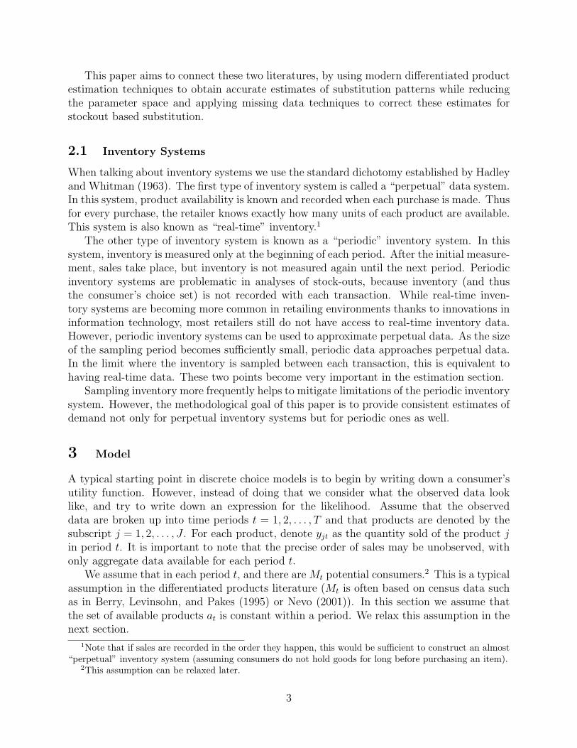
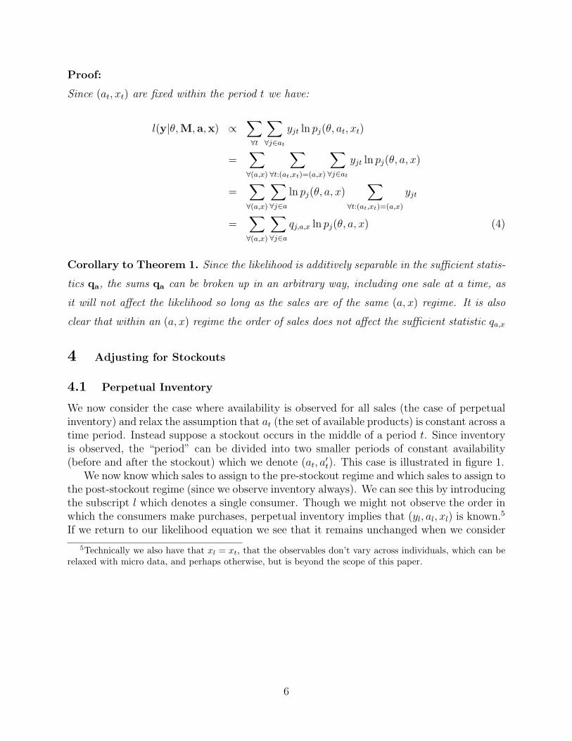
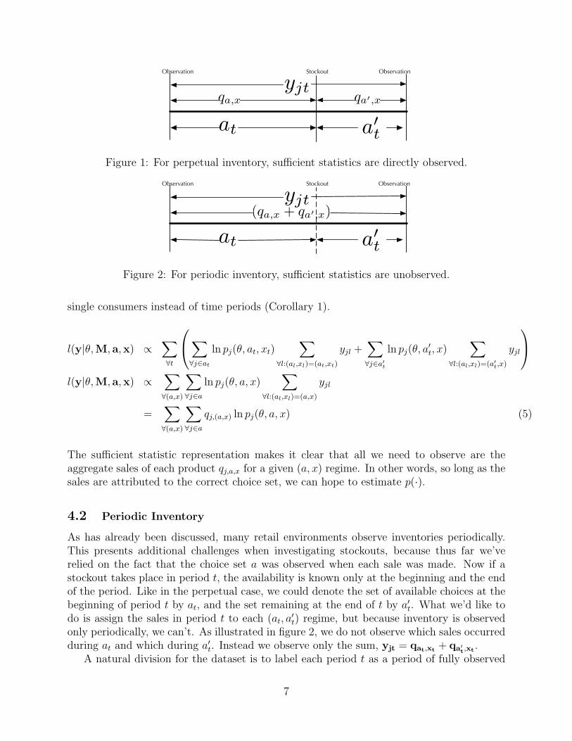
We now consider the case where availability is observed for all sales (the case of perpetualinventory) and relax the assumption that at (the set of available products) is constant across atime period. Instead suppose a stockout occurs in the middle of a period t. Since inventoryis observed, the “period” can be divided into two smaller periods of constant availability(before and after the stockout) which we denote (at, a

′t). This case is illustrated in figure 1.

We now know which sales to assign to the pre-stockout regime and which sales to assign tothe post-stockout regime (since we observe inventory always). We can see this by introducingthe subscript l which denotes a single consumer. Though we might not observe the order inwhich the consumers make purchases, perpetual inventory implies that (yl, al, xl) is known.5

If we return to our likelihood equation we see that it remains unchanged when we consider

5Technically we also have that xl = xt, that the observables don’t vary across individuals, which can berelaxed with micro data, and perhaps otherwise, but is beyond the scope of this paper.

6

a!t

at

Observation Stockout

yjtqa,x qa!,x

Observation

Figure 1: For perpetual inventory, sufficient statistics are directly observed.

a!t

at

Observation ObservationStockout

yjt(qa,x + qa!,x)

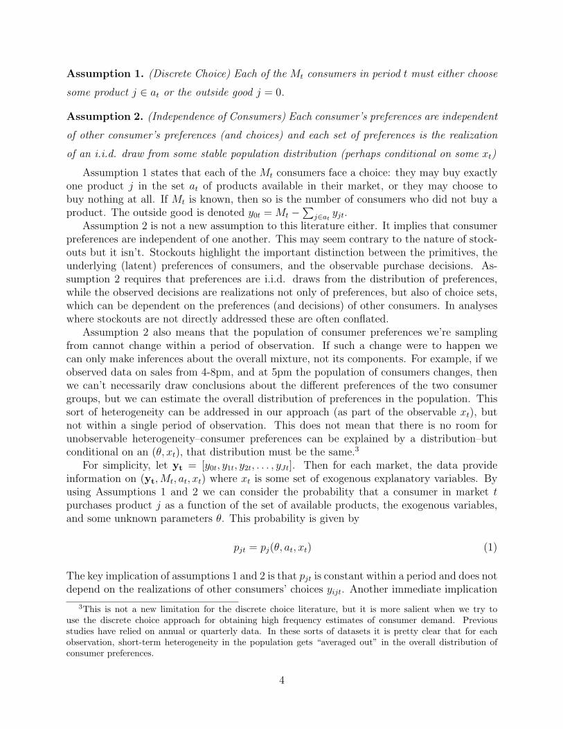
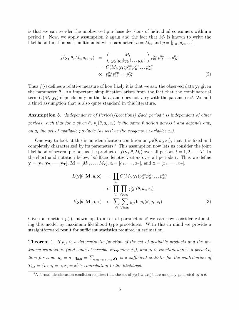
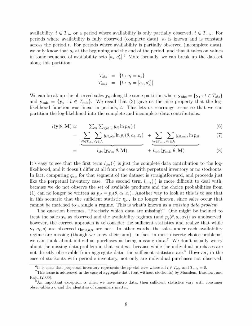
Figure 2: For periodic inventory, sufficient statistics are unobserved.

single consumers instead of time periods (Corollary 1).

l(y|θ,M, a,x) ∝∑∀t

∑∀j∈at

ln pj(θ, at, xt)∑

∀l:(al,xl)=(at,xt)

yjl +∑∀j∈a′t

ln pj(θ, a′t, x)

∑∀l:(al,xl)=(a′t,x)

yjl

l(y|θ,M, a,x) ∝

∑∀(a,x)

∑∀j∈a

ln pj(θ, a, x)∑

∀l:(al,xl)=(a,x)

yjl

=∑∀(a,x)

∑∀j∈a

qj,(a,x) ln pj(θ, a, x) (5)

The sufficient statistic representation makes it clear that all we need to observe are theaggregate sales of each product qj,a,x for a given (a, x) regime. In other words, so long as thesales are attributed to the correct choice set, we can hope to estimate p(·).

4.2 Periodic Inventory

As has already been discussed, many retail environments observe inventories periodically.This presents additional challenges when investigating stockouts, because thus far we’verelied on the fact that the choice set a was observed when each sale was made. Now if astockout takes place in period t, the availability is known only at the beginning and the endof the period. Like in the perpetual case, we could denote the set of available choices at thebeginning of period t by at, and the set remaining at the end of t by a′t. What we’d like todo is assign the sales in period t to each (at, a

′t) regime, but because inventory is observed

only periodically, we can’t. As illustrated in figure 2, we do not observe which sales occurredduring at and which during a′t. Instead we observe only the sum, yjt = qat,xt + qa′

t,xt .A natural division for the dataset is to label each period t as a period of fully observed

7

availability, t ∈ Tobs or a period where availability is only partially observed, t ∈ Tmis. Forperiods where availability is fully observed (complete data), at is known and is constantacross the period t. For periods where availability is partially observed (incomplete data),we only know that at at the beginning and the end of the period, and that it takes on valuesin some sequence of availability sets [as, a

′s].

6 More formally, we can break up the datasetalong this partition:

Tobs = {t : at = as}Tmis = {t : at = [as, a

′s]}

We can break up the observed sales yt along the same partition where yobs = {yt : t ∈ Tobs}and ymis = {yt : t ∈ Tmis}. We recall that (3) gave us the nice property that the log-likelihood function was linear in periods, t. This lets us rearrange terms so that we canpartition the log-likelihood into the complete and incomplete data contributions:

l(y|θ,M) ∝∑

∀t

∑∀j∈Jt

yjt ln pjt(·) (6)

=∑

∀t∈Tobs

∑∀j∈Jt

yjt,obs ln pj(θ, at, xt)︸ ︷︷ ︸ +∑

∀t∈Tmis

∑∀j∈Jt

yjt,mis ln pjt︸ ︷︷ ︸ (7)

= lobs(yobs|θ,M) + lmis(ymis|θ,M) (8)

It’s easy to see that the first term lobs(·) is just the complete data contribution to the log-likelihood, and it doesn’t differ at all from the case with perpetual inventory or no stockouts.In fact, computing qa,x for that segment of the dataset is straightforward, and proceeds justlike the perpetual inventory case. The second term lmis(·) is more difficult to deal with,because we do not observe the set of available products and the choice probabilities from(1) can no longer be written as pjt = pj(θ, at, xt). Another way to look at this is to see thatin this scenario that the sufficient statistic qa,x is no longer known, since sales occur thatcannot be matched to a single a regime. This is what’s known as a missing data problem.

The question becomes, “Precisely which data are missing?” One might be inclined totreat the sales yt as observed and the availability regimes (and pj(θ, at, xt)) as unobserved,however, the correct approach is to consider the sufficient statistics and realize that whileyt, at, a

′t are observed qmis,a,x are not. In other words, the sales under each availability

regime are missing (though we know their sum). In fact, in most discrete choice problems,we can think about individual purchases as being missing data.7 We don’t usually worryabout the missing data problem in that context, because while the individual purchases arenot directly observable from aggregate data, the sufficient statistics are.8 However, in thecase of stockouts with periodic inventory, not only are individual purchases not observed,

6It is clear that perpetual inventory represents the special case where all t ∈ Tobs and Tmis = ∅.7This issue is addressed in the case of aggregate data (but without stockouts) by Musalem, Bradlow, and

Raju (2006).8An important exception is when we have micro data, then sufficient statistics vary with consumer

observables xt, and the identities of consumers matter.

8

but neither are the sufficient statistics.

Incorporating Missing Data

One way to deal with a missing data problem is to to ignore lmis(·) and just do estimationon the lobs(·) part. This is akin to throwing away the observations ymis and just doingestimation when the set of available products is fully observed. There’s a large literature onwhen this strategy leads to consistent estimates (Rubin 1976) . In the multinomial case, solong as discarding the data doesn’t affect the distribution of the sufficient statistics, ignoringthe missing data should only lead to a loss of efficiency, not inconsistency.

However, it is easy to see that the sufficient statistics are affected by discarding themissing data, with the following example: Consider the product that stocks out. If it hascapacity ω, then if the data are observed we know that q < ω, and if the data are discardedwe know that q = ω. Thus the sufficient statistic clearly depends on the “missingness”of the data. Therefore, by ignoring the missing data, we would expect to systematicallyunderestimate demand for products which stock out.

Another approach is to replace lmis(·) with some consistent estimator that is computable.One can replace lmis(·) with its expectation by integrating it out over all possible values ofthe missing data. The typical notation here is:

Q(θ) = lobs(yobs, θ) + E[lmis(ymis, θ)]

It’s now possible to maximize Q(θ) by choosing the best θ via ML. By iterating back andforth between computing the expectation of lmis(·) and maximizing Q(θ), our estimate willeventually iterate to a fixed point. This is the well-known EM Algorithm. Dempster, Laird,and Rubin (1977) prove several properties about EM, namely that it consistently convergesto the ML value, and that it does so monotonically (so that each iteration between computingthe expectation of the missing data contribution and the complete data likelihood increasesthe likelihood function). We typically superscript EM iterations with k. To compute thenext iteration of the EM algorithm (k + 1), we use the estimate of θ from the kth iteration,θk, to evaluate the expectation of missing data’s contribution to the log-likelihood.

The EM algorithm has a long history in the context of multinomial likelihoods (Hartley1958), because computing the expected contribution of the missing data is straightforward.Once again, the fact that the log-likelihood is linear in the data yjt and the sufficient statisticsqa,x, simplifies the computation dramatically.

E[lmis(ymis(θk,yobs)|θk−1] = E

∑∀t∈Tmis

∑a∈{at,a′t}

∑∀j∈a

yjt,mis ln pj(θ, a, xt)|θk

=

∑∀t∈Tmis

∑at∈{at,a′t}

∑∀j∈a

E(yjt,mis|θk) ln pj(θ, a, xt) (9)

The previous equation shows that in order to evaluate the likelihood, we do not need to

9

integrate out over all possible values of the missing data, instead linearity implies we cansimply plug in the expected sufficient statistic. We can also define the augmented dataset,yaug(θ

k) = [ymis(θk),yobs], and see that the adjusted likelihood function is the same as the

likelihood function which treats the augmented dataset as the complete data (again vialinearity). Therefore it is possible to estimate the parameters θ by maximum likelihood.

θk+1 = arg maxθ

Q(θ)

= arg maxθ

lobs(yobs, θ) + E[lmis(ymis, θ)]

= arg maxθ

T∑t=1

l(θ|yaug(θk)) (10)

(This is the M-Step.)At this point, we must derive an expression for the expectation of the missing data. We

consider the case where in period t product k stocks out, and assume that Mt potentialconsumers are in our market in period t so that mt ≤ Mt of them face choice set at andMt−mt of them face choice set a′t. For notational convenience we let αt = mt

Mtbe the fraction

of consumers not affected by the stockout. It becomes clear that for some product j 6= l thatconditional on yjt the overall sales observed for that time period, the sales are distributedbinomially across the two regimes.9 In fact the number of sales before and after the stockout(for a single period) are:

qj,a,xt,t ∼ Bin

(yjt,

αtpj(θ, at, xt)

αtpj(θ, a, xt) + (1− αt)pj(θ, a′, xt)

)E[qj,a,xt,t] = yjt

αtpj(θ, at, xt)

αtpj(θ, a, xt) + (1− αt)pj(θ, a′, xt)(11)

E[qj,a′,xt,t] = yjt − E[qj,a,xt ] (12)

The last two expressions represent the contribution of the period t to the sufficient statis-tic qa.x. Given values of θ, and αt it is easy to compute these expectations. We’ve alreadydiscussed using how to update θk iteratively, so all that remains is to address αt. We don’tknow the true value of αt, and there are typically three ways to handle this. The standardE-M approach is to specify a distribution for αt and integrate it out. Another approach is toadd an additional step to our iterative procedure where we draw αt from its marginal distri-bution, and treat it as data for the E- and M-steps (this is akin to a Gibbs Sampler/MCMC).The third approach is to treat αt not as missing data, but rather as a parameter to be es-timated, and choose the value of αt which best improves the likelihood. All three of thesemethods are going to have tradeoffs between how many E-M iterations are required forconvergence and how long each iteration takes.10

9It is important to highlight that this is not an assumption. This follows representationally, from As-sumptions 1-3 and our underlying multinomial DGP.

10For a fully Bayesian MCMC approach (such as the Gibbs Sampler) we won’t actually reach a fixed point

10

The standard E-M approach is to integrate out the αt’s. Notice this is much easierthan integrating the entire likelihood, we only need to integrate to compute the (singledimensional) expectation in (11). In order to do this we must specify a distribution for αt.Consider mt is the number of consumers facing choice set at which must be determined bythe product l that stocks out. We can look at this as the number of consumers before ql,a,xt

bernoulli trials are successful given it must be less than Mt consumers. This is the definitionof the conditional negative binomial.11 Therefore we can write,

αt

Mt

= mt ∼NegBin(ql,a,xt , pl(θ, a, xt))

NegBinCDF (Mt, pl(θ, a, xt))= w (mt|ql,a,xt , Mt, pl(θ, a, xt))

Since this is a discrete distribution we can compute the expectation over all mt ≤ Mt

using the w(αt|(·)) as p.m.f. weights by taking the sum

E[qj,a,xt ] =Mt∑

mt=0

yjtmtpj(θ, at, xt)

mtpj(θ, a, xt) + (1−mt)pj(θ, a′, xt)w(mt|(·)) (13)

(This is the E-Step.)12

The other way to handle αt is to exploit the duality in the Bayesian world betweenparameters and missing data to estimate αt. We can consider the partial likelihood of eachperiod lt(·), and choose the αt which maximizes it’s contribution to the likelihood function.This is particularly convenient because αt does not effect the partial likelihood of otherperiods ls(·) for s 6= t, likewise αt only enters the E[yjt] and combinatorial terms of thelikelihood, and never any terms involving θ. That means we can divide our parameter spaceand condition out on αt when searching for θ and vice versa. Even though there are manyαt’s to find now (one for each period with missing data), the computational burden is notthat bad because it is sufficient to do several hundred single dimensional optimizations whichis orders of magnitude easier than a single large dimensional optimization problem. Thisalgorithm typically takes more time per iteration than the E-step estimator above, but feweriterations to achieve convergence. When such separation of parameter space is possible thisis a variant of the EM algorithm often referred to as ECM (Liu and Rubin 1994), and hasnatural analogues to fully Bayesian (MCMC) approaches.(This is the C-Step).13

By alternating between imputing the missing data (E-Step) and maximizing the (log)likelihoodfunction (M-Step) it is possible to obtain estimates for parameters (θ, α) which increase like-lihood monotonically until reaching a fixed point.

but rather a stationary distribution.11This is once again not an assumption on the process but rather a consequence of the multinomial DGP.12The multiple stockout case proceeds analogously, although it relies on the multivariate generalization

of the negative binomial, the negative multinomial, and involves more than one sum. The approach canbe extended to deal with many unobserved stockouts, the technical details of which are presented in theAppendix.

13This was explored in response to a comment Jack Porter made about a previous version.

11

5 Estimation

5.1 Parametrizations

All that remains is to specify a functional form for pj(α, at, xt). In this section we’ll presentseveral familiar choices and how they can be adapted into our framework. In any discretemodel, when n is large and p is small the poisson model becomes a good approximation forthe sales process of any individual product. The simplest approach would be to parameterizepj(·) in an semi-nonparametric way:

pj(θ, at, xt) = λj,at

Then, the ML estimate is essentially the mean conditional on (at, xt). This is more or lessthe approach that Anupindi, Dada, and Gupta (1998) take. The advantage is that it avoidsplacing strong parametric restrictions on substitution patterns, and the M-Step is easy. Thedisadvantage is that it requires estimating J additional parameters for each choice set at

that is observed. It also means that forecasting is difficult for at’s that are not observed inthe data or are rarely observed. It highlights issues of identification which we will addresslater.

A typical solution in the differentiated products literature to handling these sorts ofproblems is to write down a random coefficients logit form for choice probabilities. This stillhas considerable flexibility for representing substitution patterns, but avoids estimating anunrestricted covariance matrix. What’s also nice is that this family of models is consistentwith random utility maximization (RUM). If we assume that consumer i has the followingutility for product j in market t and they choose a product to solve:

arg maxj

uijt(θ)

uijt(θ) = δjt(θ1) + µijt(θ2) + εijt

Where δj is the mean utility for product j, µij is the individual specific taste, and εijt isthe idiosynchratic logit error. It is standard to partition the parameter space θ = [θ1, θ2]between the linear (mean utility) and non-linear (random taste) parameters. This functionalspecification produces the individual choice probability, and the aggregate choice probability

Pr(k|θ, at, xt) =exp[δk(θ1) + µik(θ2)]

1 +∑

j∈atexp[δj(θ1) + µij(θ2)]

This is exactly the differentiated products structure found in many IO models (Berry1994, Berry, Levinsohn, and Pakes 1995). These models have some very nice properties. Thefirst is that any RUM can be approximated arbitrarily well by this “logit” form (McFaddenand Train 2000). This also means that the logit (µij = 0) and nested logit models can benested in the above framework. For the nested logit, µijt =

∑g σgζjgνig, where ζjg = 1 if

12

product j is in category g and 0 otherwise, and νig is standard normal. For the randomcoefficients logit of BLP, µijt =

∑l σlxjlνil, where xjl represents the lth characteristic of

product j and ν is standard normal. In both models, the unknown parameters are theσ’s. This representation makes it clear that the nested logit is a special case of the randomcoefficients logit.

The second advantage of these parametrizations is that it is easy to predict choice prob-abilities as the set of available products changes. If a product stocks out, we simply adjustthe at in the denominator and recompute. A similar technique was used by Berry, Levin-sohn, and Pakes (1995) to predict the effects of closing the Oldsmobile division and by Petrin(2002) to predict the effects of introducing the minivan. The parsimonious way of addressingchanging choice sets is one of the primary advantages of these sorts of parameterizations,particularly in the investigation of stockouts.

When there is sufficient variation in the choice set, Nevo (2000) shows that productdummies may be used to parameterize the δjt’s. When we include product dummies itallows us to rewrite the δ’s as:

δjt = Xjβ + ξj︸ ︷︷ ︸ +ξt + ∆ξjt

= dj +ξt + ∆ξjt (14)

where dj functions as the product “fixed-effect”. If we have enough observations, we canalso include market specific effects to capture the ξt. This changes the interpretation ofthe structural error ξ, which is traditionally the unobservable quality of the good. Theremaining error term ∆ξjt is the market specific deviation from the mean utility. Nevo(2000) points out that the primary advantage is that we no longer need to worry about theprice endogeneity and choice of instruments inside our optimization routine, while the meantastes for characteristics β (along with the ξj’s) can be captured by a second-stage regressionof dj on Xj.

This highlights some important consequences for our study of stockouts. We expectproducts which stock out to have higher than average ξjt’s. Therefore, if we discard datafrom periods where stockouts occur, this is akin to violating the moment condition on ∆ξjt

as we are more likely to discard data from the right side of the distribution than the left.14

Likewise, if we estimate assuming full availability, stocked out products should have largenegative ∆ξjt’s (since they have no sales at all), which once again violates the momentcondition on ∆ξjt.

5.2 Heterogeneity

Thus far, we’ve done everything conditional on xt. In one sense, this is useful to show that ourresult holds for the case of conditional likelihood, but it is also of practical significance to ourapplied problem. Since periods in our dataset are short, it is likely that choice probabilitiesmay vary substantially over periods. Over long periods of time (such as annual aggregate

14This correlation may not be as strong as one might expect because stockouts are also correlated withlow inventory, which should be uncorrelated (perhaps even slightly negatively) with ∆ξjt.

13

data) these variations get averaged out. The distribution of tastes over a long period isessentially the combination of many short-term taste distributions. We only observe whatwe estimate, so usually that is the long run distribution. With high frequency data we areno longer so limited and can address this additional heterogeneity by conditioning on xt. Wemight think that xt includes information such as the time of day, day of the week, or locationidentifiers. Depending on how finely data are observed, not accounting for this additionalheterogeneity may place a priori unreasonable restrictions on data.

We can model this dependence on xt in several ways. One is to treat p(·|xt) as a differentfunction for each xt. In other words we could think about each location having its owndistribution of tastes, and parameters θ. We could also imagine a scenario where all marketsfaced the same distribution of consumers, but that distribution varied depending on the dayof the week. In this approach xt can be thought of as the demographic covariates used inthe differentiated products literature (Petrin 2002, Nevo 2000), or as consumer level micro-data (Berry, Levinsohn, and Pakes 2004), but need not be limited as such. Another way wecould think about the xt are as characteristics of consumers. Some of the parameters in θmight be fixed over xt’s while others depend on xt. A good example might be to think thatthe correlation of tastes is constant across all populations but the mean levels are different.When we present the estimates we explore several different such dimensions of heterogeneity.

The other approach we can take is to parameterize M , based on information similar to theinformation we’ve incorporated in the xt’s. Thus instead of letting the choice probabilitiesvary, we could let the number of consumers passing by the machine vary. This becomeshelpful because M is going to be the driving force behind substitution to the outside good.It also allows for a common shock across periods without affecting the choice probabilities. Inmarkets with retail data, this can be extremely useful as a way of adjusting for seasonality,holidays, or other events which might have an affect on the effective size of the market.Parameterizing M has a long history in the literature (Berry 1992). In practice, it’s prettyeasy, and can be considered as a (C-Step). At each iteration we simply find the parametervalues for M which maximize the likelihood conditional on the (θ, α). We don’t worryabout simultaneity because the likelihood factors in M . Once again this approach begins toresemble a fully Bayesian MCMC approach. We present some specifications for M with theestimates.

5.3 Identification of Discrete Choice Models

In this section we address non-parametric and parametric identification of the choice proba-bilities pj(θ, at, xt), while still continuing to assume the underlying d.g.p. is multinomial. Thegoal is not to provide formal identification results, but rather to provide a clear expositionso that the applied researcher can better understand the practical aspects of identificationin the discrete choice context. For the quite general formal results, the standard reference isMatzkin (1992).15

15Athey and Imbens (2006) provide some related identification results for the fully Bayesian MCMCestimator for these sorts of models. As already discussed our approach could be computed using such anMCMC approach as well.

14

Nonparametric identification is easily addressed by our qa,x sufficient statistic representa-tion. For a given (a, x), the sufficient statistics must be observable, moreover the efficiencyis roughly going to go as

√na,x where na,x are the total number of consumers facing (a, x).

Unless every (a, x) pair in the domain is observed (and with a substantial number of con-sumers) the conditional mean (semi-nonparametric) representation of our pj(θ, at, xt)’s willmost likely not be nonparametrically identified.

Typically we use the random coefficients parameterization presented above, so we’re moreworried about whether that is going to be parametrically identified. One approach mightbe to assume a smooth functional form for pj(·) and then use delta method arguments todo a change of variables to the parameterized version, but a heuristic sufficient statisticsbased argument may be easier to understand (and hopefully more useful) for the appliedresearcher.

The typical source of identification in the differentiated products literature is by long runvariation in the choice set. For this to be useful as a source of identification, these variationsmust be exogenous to the model. Thus we could think about each “observation” as beingthe qa,x sufficient statistics we’ve presented in this paper. The way to think about thesemodels is to compute the effective number of qa,x “observations” and compare them to theparameters we’re hoping to explain. We can see this by constructing a matrix of observableswhich describes each qa,x. In many discrete choice models these may be characteristics,product dummies, time dummies, of the available products. For nonlinear effects, (tastes forexample), interaction terms should also be included. If we want to see if we can estimate allof those parameters, we could think about determining whether or not our “data” matrix isof full-column rank. We also see that many of our observations will have the same descriptivevariables, and thus will be linearly dependent. Once again the qa,x representation makes thisquite clear, as we don’t have additional observations but rather our additional observationsget added into the sum of qa,x (which may improve efficiency but not allow us to identifyadditional parameters). Stockouts are useful, particularly when trying to identify productdummies, because they provide linearly independent observations of qa,x. If we only everobserve a change from choice set a → a′ (suppose the only product that ever stocks out isSnickers), then we only have two effective “observations”. If we observe lots of stockoutsand different choice sets, then we have the potential to observe J × (J − 1) “observations”.

In Berry, Levinsohn, and Pakes (1995) and related literature the choice set is not acollection of products but rather a collection of bundles of characteristics. Thus their at

is not the set of available products j = 1, . . . , J as it is in our model, but rather the setof available characteristics at = {∀j ∈ t : zj} (including price), for each product. This isimportant because the primary source of identification comes from variations in one of thecharacteristics, price, across time and markets. When price changes from one period to thenext, this represents a change in the at, albeit usually only along a single dimension of zj.Other sources of variation in the choice set involve changes in product characteristics asthey vary from year to year (mileage, HP, etc.). The third source of choice set variation iswhen new goods are introduced, and an entirely new zj is provided to consumers. A possibledisadvantage to applying the technique of BLP to other industries is that there may notbe sufficient variation in the characteristics of products from one year to the next, or thatvariation (changes in characteristics and product mix) is often endogenously determined by

15

the participants.Our model presents a different way to interpret variation in choice sets. In our context

at doesn’t vary with long term product mix, or potentially endogenous pricing decisions,but rather as products stock out. When products stock out they are no longer in the setof available products at. This variation is potentially more useful because our new choiceset does not necessarily look like the old choice set with a single dimension of zj altered.Instead, we add and remove entire zj’s similar to the new products case. This is particularlyhelpful, because it allows us to observe substitution not on a single characteristic at a time,but jointly over several characteristics. Moreover, when stockouts happen one at a time,we know which joint distribution to attribute those changes to. Using long-term variation,product mixes vary roughly simultaneously from model year to model year.

Additionally, this variation is 100% exogenous as we’ve written down our model, becausefirms take changes in consumer’s choice sets as given, and so do consumers. This mightnot seem obvious at first, but because choice sets are realizations of stochastic choices ofconsumers, and consumers choices depend only on the set of available products, stockoutsare random events. While firms can restock the machine (or even change the product mixto prevent future stockouts), this does not change the fact that any particular stockout isexogenous to the model.

Finally, one of the most common applications of these sorts of models is to predict substi-tution probabilities. It should be clear that the best way to predict substitution probabilitiesis to observe them. Stockouts provide not only a chance to observe substitution probabil-ities, but also an opportunity to observe them repeatedly and across different dimensionsthan previous approaches have been able to.

5.4 Computation

So far, the M-step has been presented in the context of maximum likelihood (ML), or in thecase where random coefficients are used maximum simulated likelihood (MSL). The algo-rithm for these approaches would be to simulate consumers, compute the choice probabilities,and evaluate the likelihood.

It is important to recognize that by using the EM algorithm or one of its variants we arenot locked into ML estimation. A typical approach to the demand side in a differentiatedproducts setting is to iterate on the contraction mapping from Berry, Levinsohn, and Pakes(1995). This is particularly effective because it solves for the unique set of optimal δ’s mono-tonically without computing anything other than choice probabilities. More importantly thefit is exact and unique. A further advantage of GMM approaches over ML is the ability toincorporate additional (structural) moments along with the demand side.16

A GMM approach using demand-side moments can be used in lieu of ML estimationin the M-step. In fact, the Generalized EM algorithm (GEM) Dempster, Laird, and Rubin(1977) says that any approach which improves the log-likelihood at each EM iteration (ratherthan fully maximizing the likelihood of the augmented dataset) will converge to the correct

16Draganska and Jain (2004) develop a method for incorporating supply side information in the MLframework which appears to be agreeable with the missing data procedure we’ve provided.

16

value. In other words it is sufficient that θ is any sequence which obeys:

l(θ(k+1),yaug(θ

(k)))≥ l

(θk,yaug(θ

(k−1)))

(15)

should lead to consistent EM corrected estimates.Therefore, we can replace the ML estimator in the M-step, with the easier to compute

GMM estimator from Berry, Levinsohn, and Pakes (1995) as long as we verify that thecondition (15) holds at each step, it is perfectly acceptable to use δ’s obtained from thecontraction mapping of BLP rather than obtaining ML estimates. Typically the contractionmapping in Berry, Levinsohn, and Pakes (1995) is written as

δ(n+1)j = δ

(n)j + ln(sj)− ln pj(θ, at, xt)

However, E[ln pj(θ, at, xt)] is not linear in the missing data, and computing could be tricky.This is easily remedied as the standard computational trick is to use the exponentiated δ’sin the contraction mapping and then we have that:

exp(δ(n+1)j ) = exp(δ

(n)j )

qj

qj,at,xt(θ)

While optimizing the likelihood function can be expensive (particularly if simulation isrequired), evaluating is relatively cheap. Once this condition fails to hold, a switch to MLestimates should be made just to check convergence, but in most cases an additional MLiteration does not improve the overall likelihood.17

A useful way to think about what the EM adjustment does is to note that there aresome missing data regarding which products are available. Without knowledge that matchessales to the sets of available products, the values for δ are incorrect. The EM algorithm usesobservable information about the substitution patterns to replace unknown δ’s with moreaccurate estimates, and then recomputes estimates for the parameters. All other algorithms(GMM, ML, MH, Gibbs Sampling) are simply ways to get to the maximum. For the resultswe report later, we use GMM. Details for the exact moment conditions used are containedin the Appendix.

17This is a result of the exact fit of the δ’s in the BLP moments, and the fact that we don’t includesupply side moments. If supply side moments are included we don’t expect ML and GMM to give the sameestimates. In this scenario, the EM-GMM estimates are probably appropriate. The problem is that we aren’taware of a broad theoretical result for incorporating missing data in moment condition models as Dempster,Laird, and Rubin (1977) do for ML.

17

6 Industry Description, Data, and Reduced-form Results

6.1 The Vending Industry

The vending industry is well suited to studying the effects of product availability in manyrespects. For one, product availability is well defined. Products are either in-stock or not(there are no extra candy bars in the back, on the wrong shelf, or in some other customer’shands). Likewise, products are on a mostly equal footing (no special displays, promotions,etc.). The product mix, and layout of machines is uniform across all of the machines in thesample and for the most part remains constant over time. Thus most of the variation in thechoice set comes from stockouts, which are a result of stochastic consumer demand ratherthan the possibly endogenous firm decisions to set prices and introduce new brands.18

Typically a location seeking vending service requests sealed bids from several vendingcompanies for contracts that apply for several years. The bids often take the form of a two-part tariff, which is comprised of a lump-sum transfer and a commission paid to the ownerof the property on which the vending machine is located. A typical commission rangesfrom 10 − 25% of gross sales. Delivery, installation, and refilling of the machines are theresponsibility of the vending company. The vending company chooses the interval at whichto service and restock the machine, and also collects cash at that interval. The vendingcompany is also responsible for any repairs or damage to the machines. The vending clientwill often specify the number and location of machine. Sometimes the client specifies aminimum number of machines and locations, and several optional machines and locations.

Vending operators may own several “routes” each administered by a driver. Driversare often paid partly on commission so that they maintain, clean, and repair machines asnecessary. Drivers often have a thousand dollars worth of product on their truck, and a fewthousand dollars in coins and small bills by the end of the day. These issues have motivatedadvances in data collection, which enable operators to not only monitor their employees,but also to transparently provide commissions to their clients and make better restockingdecisions.

In order to measure the effects of stock-outs, we use data from 58 vending machines onthe campus of Arizona State University (ASU). This is a proprietary dataset acquired fromNorth County Vending with the help of Audit Systems Corp (later InOne Technologies, nowStreamware Inc.). The data were collected from February-June 2003, which correspondswith the spring term at ASU.

Each of these machines collects Digital Exchange (DEX) data. DEX is the vendingindustry standard data format, and was originally developed for handheld devices in theearly 1990’s. In a DEX dataset, the machine records the number and price of all of theproducts vended. The data are typically transferred to a hand-held device by the routedriver while he services and restocks the machine. This device is then synchronized with acomputer at the end of each day. In our dataset, (thought not typically) additional inventoryobservations are made between service visits, because DEX data are wirelessly transmittedseveral times each day. As of 2003, the ASU route was the only route to be fully wireless

18In this sense, our setup is substantially simpler than that of Nevo (2001) or Berry, Levinsohn, and Pakes(1995) where new brands and prices are substantial sources of identification.

18

enabled.

6.2 Data Description

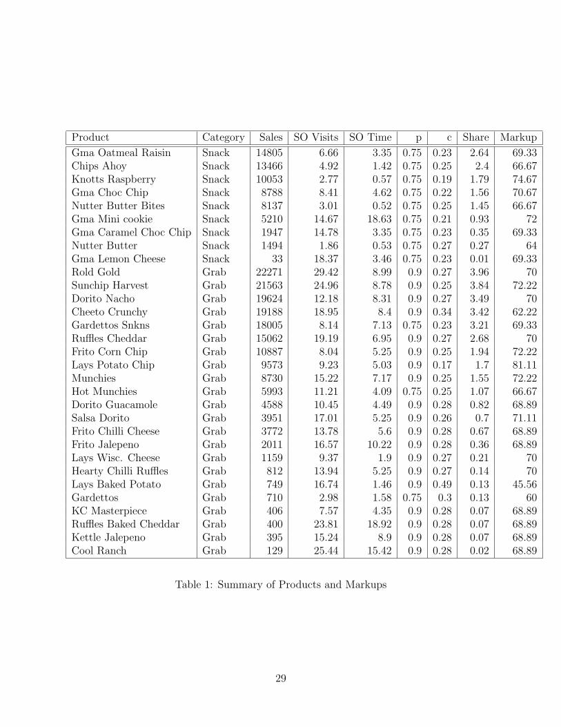
The dataset consists of snack and coffee machines; we focus on the snack machines in thisstudy. Throughout the period of observation, the machines stock around 70 different prod-ucts, including chips, crackers, candy bars, packaged donuts, gum, and mints. Some productsare present only for a few weeks, or only in a few machines. Of these products, some of themare non-food items 19 or have insubstantial sales (usually less than a dozen total over allmachines). In the examples we present, we exclude these items in addition to excluding gumand mints, based on the assumption that these products are substantially different frommore typical snack foods, and rarely experience stockouts. Including gum and mints doesnot substantially change our results. It is important to note that not every product appearsin every machine. The 50 products in the dataset are listed in Tables 1 and 2.

Typically, sales are only observed when vending machines are refilled. Thus in order tohave data before and after a change in product availability occurs, “perpetual” data collectionwould be required. The data from Arizona State University are interesting because periodicwireless readings of the inventory data are observed each day (often several times). Thisprovides two distinct advantages: the observation of the machine is no longer linked to therestocking of the machine,20 and the machine’s inventory is sampled more frequently. Thesehelp to mitigate the limitations of the periodic inventory system. The methodological goalof this paper is to provide consistent estimates of demand not only for perpetual inventorysystems but for periodic ones as well.

In addition to the sales, prices, and inventory of each product, we also observe productnames, which we link to the nutritional information for each product in the dataset. Forproducts with more than one serving per bag, the characteristics correspond to the entirecontents of the bag. This is somewhat similar to the approach taken by Nevo (2000) forRTE cereal.

The retail prices observed in the vending machine are constant over time and acrossbroad groups of products as shown in Tables 1 and 2. Baked goods typically vend for$1.00, chips for $0.90, cookies for $0.75, candy bars for $0.65, and gum and mints for $0.60.This makes for a simpler and less complicated framework for static models of demand. Ascompared to typical studies of retail demand and inventories (which often utilize supermarketscanner data), there are no promotions or dynamic price changes (Aguirregabiria 1999). Thispresents a bit of a problem, because for the most part prices do not vary within a particularproduct category. This means that once most product characteristics (and certainly productor category dummies) are included, price effects are not identified. The method we presentwill work fine in cases where a price coefficient is identified, but in our particular empirical

19While often sold alongside of snacks in vending machines, condoms are poor substitutes for potato chips,and are not included in our sample.

20This is not exactly true. While a wireless observation can be made without restocking the machine, thewireless readings are also available to the vending company, and thus decisions to refill are endogenous. Fora static analysis of stock-outs that is not concerned with the retailer’s dynamic restocking problem, this isnot problematic.

19

example this is not the case.The dataset also contains stockout information and marginal cost data (the wholesale

price paid by the firm) for each product. The stockout percentage is the percentage of servicevisits at which the product is observed to have stocked-out. This number will be higher thanthe percentage of time in which the product is stocked out, because stock-outs may occurshortly before a service visit. The marginal cost data are consistent with available wholesaleprices for the region. There is slight variation in the marginal costs of certain products, whichmay correspond to infrequent re-pricing by the wholesaler. The median wholesale prices foreach products are listed in Tables 1 and 2. By examining Tables 1 and 2, several trendsbecome apparent. There is a lot of variation in the markups of the products. Markups arelowest on branded candy bars (about 50%), and markups are highest on the Big GrabTMchips(about 70%). The product with the highest markup is the Peter Pan crackers, which havean average markup of nearly 82%. Table 3 reports regression estimates from a regressionof markup on the percentage of the time a product is stocked out. The result shows whatone might expect; namely that products with high markups are less likely to stock out thanproducts with lower markups. This is also true when product category is adjusted for.

Other costs of holding inventory are also observed, including the spoilage and numberof products removed from machines. Spoilage does not constitute more than 3% of mostproducts sold. The notable exceptions are the Hostess products, which are baked goodsand have a shorter shelf life (approximately 2 weeks) than most products, which may lastseveral months before spoiling. For this static analysis of demand, we assume that the costsassociated with spoilage are negligible.

6.3 Reduced-form Results

Before applying the estimation procedure described above to the dataset, first consider asimple reduced form analysis of stockouts. Table 4 reports the results of a regression ofstockout rates on starting inventory levels. We report results for Probit and OLS with andwithout product fixed effects. What we find is not surprising, namely that an additionalunit of inventory at the beginning of a four hour period reduces the chance of a stockout inthat product by about 1 − 2%. The fixed effects probit indicates a more substantial effectof about 7% per unit of inventory. A full column of potato chips usually contains about 14units. This means that the OLS (fixed effects) probability of witnessing a stockout from afull machine in a four hour period is .277− .011 ∗ 14 = 12%. For a machine with a startinginventory of only two units, the predicted chances of a stockout are one in four.

In table 5, we compute the average hourly profits for each four hour wireless time period.Then, we regress that on the number of products stocked out. The first specification (Column1) estimates the hourly cost to be about $0.05 per product stocked out. Since the number ofproducts stocked out across the entire machine might not matter as much as the number ofproducts stocked out in each category, we include category by category stockouts in Column4. These estimate the costs per stockout at around $0.11 per Big Grab bag of chips to $0.55per bag snack. Column 2 examines the effect of a stockout in the category with the moststockouts and estimates this effect to be about $0.66 per hour. Columns 3 and 5 also includeindicators for the number of products stocked out in the category with the most stockouts.

20

All of these regressions are clearly endogenous, and may be picking up many other factors,but they suggest some empirical trends that can be explained by the full model. Namely,stockouts decrease hourly profits as consumers substitute to the outside good, and multiplestockouts among similar products causes consumers to substitute to the outside good evenfaster.

7 Empirical Results

For the discrete choice model, several different specifications are addressed. The logit, nestedlogit, and random coefficients logit models are estimated with the assumption that themissing data are ignored. The nested logit and random coefficients model are also estimatedwith the proposed correction for missing data. Finally, the random coefficients model isalso estimated under the assumption of full product availability. An aside, that should bepointed out is that there is no missing data corrected logit model. The IIA property of thelogit model implies that the missing data is perfectly ignorable. In fact, removing a productfrom the product mix and re-estimating is a typical specification test for the standard logitmodel.

There are a number of ways in which we could condition on observable characteristics.We could run everything machine-by-machine, or pool the data from different machines.[Add discussion of the trade-offs of different conditioning decisions in estimation, and resultsof robustness tests...] The results that follow pool across machines case, the linear term is aproduct dummy (dj) and Mt is modelled as a machine fixed effect. We include all observablecharacteristics in the nonlinear part.

Table 7 reports the corrected values of many of the product dummies (the dj’s) undereach of the different models.21 As most products experience stock-outs, the correction forstock-out events tends to increase the estimate of the dj’s for each product. Naturally, ifa product experiences stock-outs only when other products are stocked-out, this correctioncan go the other way (i.e., the bias from forced substitution exceeds the bias from censoring),as we see in the case of Peter Pan Crackers. (More on this to come....)

The estimated values of the non-linear paramaters (σ’s), and the results of the second-stage regression of the dj’s on characteristics (including the R2 from this regression) arereported in Table 6. Getting the δjt’s and hence dj’s corrected means substantially dif-ferent estimates from the ignore missing data and full availability case for the mean tasteparameters.

Tables 8, 9, 10, 11 and 12 are all currently from the same representative machine. Weare re-running some of these with more to come soon.

Tables 13 and 14 present robustness tests and comparisons of different specifications forthe heterogeneity across machines and time periods. Table 13 examines heterogeneity whereestimates are conditional xt, and Table 14 presents the effects of parametrizing M . In eachtable the mean square error (MSE) is computed and the percentage of variation explainedas compared to an unrestricted model is also reported. The interpretation is meant to besimilar to an R2 which obviously doesn’t exist for this model.

21A few dj ’s were excluded just to keep the table intact, but they follow the same pattern.

21

8 Counterfactual Experiments

These estimates are now used to predict the effect that stockouts have on the profits of thevending operator. For simplicity, the model was estimated using data from a single snackmachine located in Alumni Hall on the campus of Arizona State University. This machine waschosen because it was relatively high sales volume, and was not located particularly close tothe other machines in the dataset. Two different availability regimes were compared, underthe first availability regime (labeled A), it was assumed that the product most likely tostockout from each category was stocked out. Under the second availability regime (labeledB), three popular types of chips: Big Grab Doritos, Big Grab Rold Gold Pretzels, andBig Grab Sunchips Harvest Cheddar were assumed to have stocked out. By comparing theseavailability regimes with a full availability regime, it is possible to computed expected loss tothe producer in (p−c) terms. Furthermore, it is estimated that approximately 382 consumers“consider” a purchase from the vending machine each hour22 though many choose to purchaseno product at all. Simulations are performed to obtain estimated sales under regime A andB, and they are compared to simulations of sales at the full machine using the specificationsfor demand in A,B, and the full machine. Table 11 reports the expected lost profits whencompared to the full machine with the same specification for demand. The results in Table11 indicate that the specification which assumes full availability always predicts the lowestprofit loss, and the EM corrected model predicts the most, and twice as much as the fullavailability specification. When these quantities are compared with accounting data on theamount of cash collected from the machine (about $150/week) the loss from stockouts issubstantial. Table 12 examines stockout regime B under different numbers of consumers, inan attempt to demonstrate the different curvature of the cost of stockouts. (It is importantto remember that many consumers still prefer the outside good).

Tables 13 and 14 examine the variation in the marketsize Mt and the observed sales qjt,to provide some insight as to how to model heterogeneity in our empirical example. Weused a nonparametric approach (conditional means) to predict each cell in the dataset. Wereported the mean-squared-error of the predictions, as well as the adjusted (for parametersand degrees of freedom) R2 and the implicit number of parameters involved in using thatapproach. We found that simply accounting for the time of day, or day of week with 6 or7 dummy variables respectively did an excellent job explaining the overall variation in thesize of the market. This indicates that the overall size of the market varies more across timethan across machine locations.

Likewise, the inclusion of product dummies accounted for nearly 99% of the variation inthe observed sales. Controlling for machine location, or time specific effects added complexitywithout improving the result. This indicates that sales of individual products depend mostlyon the product’s identity, and much less on which machine it is in or what time of day it is.This indicates that we can probably pool our high frequency data across time (and locations)without worrying about ignoring some important source of heterogeneity.

22between 12pm-4pm on weekdays

22

9 Conclusion

This paper has demonstrated that failing to account for product availability correctly canlead to biased estimates of demand, and that these biased estimates can lead to economicallymeaningful results when trying to measure the welfare costs of stockouts. Rather thanexamining the effect of changing market structure (entry, exit, new goods, mergers, etc.) onmarket equilibrium outcomes, we seek to understand the effect that temporary changes tothe consumer’s choice set have on producer profits (and our estimators). The differentiatedproducts literature in Industrial Organization has used long term variations in the choice setas an important source of identification for substitution patterns, this paper demonstratesthat it is also possible to incorporate data from short term variations in the choice set toidentify substitution patterns, even when the changes to the choice set are not fully observed.Finally, the welfare impact of stockouts in vending machines has been shown to have asubstantial effect on firm profits indicating that product availability may be an importantstrategic and operational concern facing firms and driving investment decisions.

23

A Estimation Details and the Case of Multiple Stockouts

A.1 Estimation Details

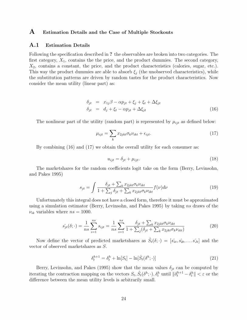
Following the specification described in ? the observables are broken into two categories. Thefirst category, X1, contains the the price, and the product dummies. The second category,X2, contains a constant, the price, and the product characteristics (calories, sugar, etc.).This way the product dummies are able to absorb ξj (the unobserved characteristics), whilethe substitution patterns are driven by random tastes for the product characteristics. Nowconsider the mean utility (linear part) as:

δjt = x1jβ − αpjt + ξj + ξt + ∆ξjt

δjt = dj + ξt − αpjt + ∆ξjt (16)

The nonlinear part of the utility (random part) is represented by µijt as defined below:

µijt =∑

k

x2jktσkνikt + εijt. (17)

By combining (16) and (17) we obtain the overall utility for each consumer as:

uijt = δjt + µijt. (18)

The marketshares for the random coefficients logit take on the form (Berry, Levinsohn,and Pakes 1995)

sjt =

∫δjt +

∑k x2jktσkνikt

1 +∑

j δjt +∑

k x2jktσkνikt

f(ν)dν (19)

Unfortunately this integral does not have a closed form, therefore it must be approximatedusing a simulation estimator (Berry, Levinsohn, and Pakes 1995) by taking ns draws of theνik variables where ns = 1000.

sjt(δ; ·) =1

ns

ns∑i=1

sijt =1

ns

ns∑i=1

δjt +∑

k x2jktσkνikt

1 +∑

j(δjt +∑

k x2jktσkνikt)(20)

Now define the vector of predicted marketshares as St(δ; ·) = [s1t, s2t, . . . sJt] and thevector of observed marketshares as S.

δh+1t = δh

t + ln[St]− ln[St(δh; ·)] (21)

Berry, Levinsohn, and Pakes (1995) show that the mean values δjt can be computed by

iterating the contraction mapping on the vectors St, St(δh; ·), δh

t until ‖δh+1t − δh

t ‖ < ε or thedifference between the mean utility levels is arbitrarily small.

24

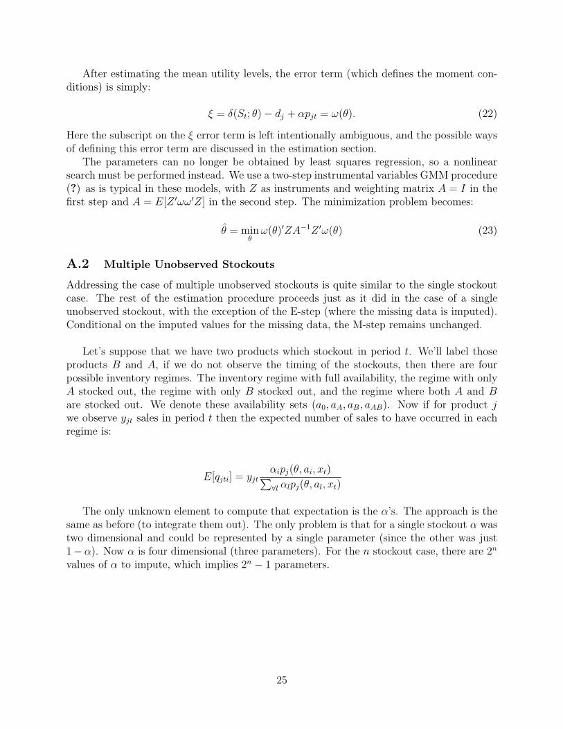
After estimating the mean utility levels, the error term (which defines the moment con-ditions) is simply:

ξ = δ(St; θ)− dj + αpjt = ω(θ). (22)

Here the subscript on the ξ error term is left intentionally ambiguous, and the possible waysof defining this error term are discussed in the estimation section.

The parameters can no longer be obtained by least squares regression, so a nonlinearsearch must be performed instead. We use a two-step instrumental variables GMM procedure(?) as is typical in these models, with Z as instruments and weighting matrix A = I in thefirst step and A = E[Z ′ωω′Z] in the second step. The minimization problem becomes:

θ = minθ

ω(θ)′ZA−1Z ′ω(θ) (23)

A.2 Multiple Unobserved Stockouts

Addressing the case of multiple unobserved stockouts is quite similar to the single stockoutcase. The rest of the estimation procedure proceeds just as it did in the case of a singleunobserved stockout, with the exception of the E-step (where the missing data is imputed).Conditional on the imputed values for the missing data, the M-step remains unchanged.

Let’s suppose that we have two products which stockout in period t. We’ll label thoseproducts B and A, if we do not observe the timing of the stockouts, then there are fourpossible inventory regimes. The inventory regime with full availability, the regime with onlyA stocked out, the regime with only B stocked out, and the regime where both A and Bare stocked out. We denote these availability sets (a0, aA, aB, aAB). Now if for product jwe observe yjt sales in period t then the expected number of sales to have occurred in eachregime is:

E[qjti] = yjtαipj(θ, ai, xt)∑∀l αlpj(θ, al, xt)

The only unknown element to compute that expectation is the α’s. The approach is thesame as before (to integrate them out). The only problem is that for a single stockout α wastwo dimensional and could be represented by a single parameter (since the other was just1−α). Now α is four dimensional (three parameters). For the n stockout case, there are 2n

values of α to impute, which implies 2n − 1 parameters.

25

E[qjti] =∑

∀αA,αB ,αAB ,α0:α0+αA+αB+αAB=1

yjtαipj(θ, ai, xt)∑∀l αlpj(θ, al, xt)

g(αA, αB, αAB, α0|θ, yjt)

E[qjti] =∑

∀αi:∑

αi=1

yjtαipj(θ, ai, xt)∑∀l αlpj(θ, al, xt)

g(α|θ, yjt)

where αl = [α0, αA, αB, . . . , αAB, . . .] is a vector of the appropriate 2n α values.All that remains is to write down the joint distribution g(α|θ, yjt). We show how to

construct the joint density g(·) for the two stockout case, but it should be clear that thisapproach can be easily extended to construct the joint density for the n stockout case. Thereare two possible sequences of availability regimes R : a0 → aA → aAB or S : a0 → aB →aAB. We can affix a probability to each sequence (with some abuse of notation), we definezR = Pr(a0 → aA → aAB) and zS = Pr(a0 → aB → aAB). It happens here that zA = 1− zB

but everything we’ve written can be extended to n stockouts.Now let’s condition on the assumption that event R actually took place, we write mA,R,t =

αA,RMt for convenience, we’ll drop the t subscripts and focus only on a single time period.Then we write m0,R = α0,RM , mA,R = αA,RM mAB,R = αAB,RM and as the number ofconsumers that would have faced regimes a0, aA, aAB respectively if event R had occurred.We also need to define the beginning of period inventories ωt = [ωAt, ωBt, . . .]. Once againfor convenience we drop t subscripts. With everything now defined, we can write down theprobabilities conditional on R.

Pr(M0,R = m0,R, MA,R = mA,R, MAB,R = mAB,R|XA = ωA, XB = ωB)

= Pr(m0,R|XA = ωA, XB = xB,0) · Pr(mA,R|XB,A = ωB − xB,0) · Pr(mAB,R = M − mA,R − m0,R)

There are three parts. The third part is trivial, the probability is one so long as M ≥mA,R + m0,R and zero otherwise. The second is the negative binomial, and the first is the

negative multinomial. We can rewrite as follows:

Pr(m0,R, mA,R, mAB,R, R) = Pr(m0,R|XA = ωA, XB = xB,0) · Pr(mA,R|XB,A = ωB − xB,0)

Pr(m0,S , mB,S , mAB,S , S) = Pr(m0,S |XB = ωB , XA = xA,0) · Pr(mB,S |XA,B = ωA − xA,0)

Because R and S have be constructed as mutually exclusive events we can add their

probabilities.

h(m0, mA, mAB , mB) = Pr(m0,R|XA = ωA, XB = xB,0) · Pr(mA,R|XB,A = ωB − xB,0)

+ Pr(m0,S |XB = ωB , XA = xA,0) · Pr(mB,S |XA,B = ωA − xA,0)

26

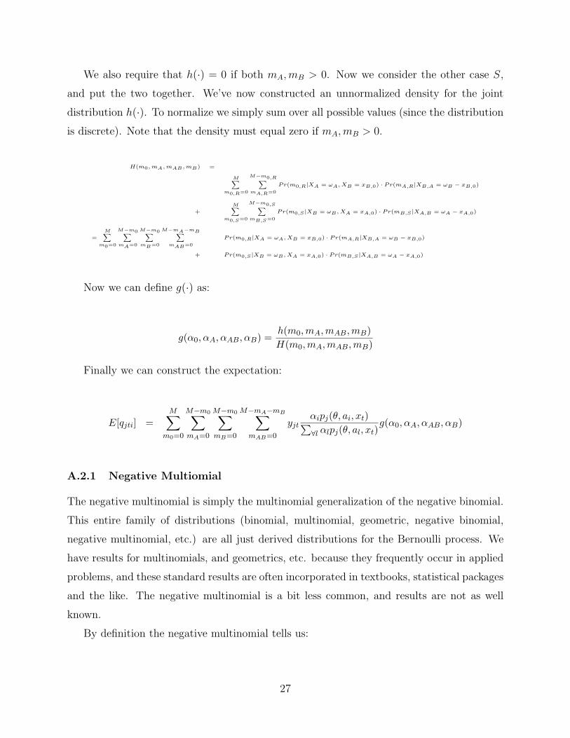
We also require that h(·) = 0 if both mA, mB > 0. Now we consider the other case S,

and put the two together. We’ve now constructed an unnormalized density for the joint

distribution h(·). To normalize we simply sum over all possible values (since the distribution

is discrete). Note that the density must equal zero if mA, mB > 0.

H(m0, mA, mAB , mB) =

M∑m0,R=0

M−m0,R∑mA,R=0

Pr(m0,R|XA = ωA, XB = xB,0) · Pr(mA,R|XB,A = ωB − xB,0)

+M∑

m0,S=0

M−m0,S∑mB,S=0

Pr(m0,S |XB = ωB , XA = xA,0) · Pr(mB,S |XA,B = ωA − xA,0)

=M∑

m0=0

M−m0∑mA=0

M−m0∑mB=0

M−mA−mB∑mAB=0

Pr(m0,R|XA = ωA, XB = xB,0) · Pr(mA,R|XB,A = ωB − xB,0)

+ Pr(m0,S |XB = ωB , XA = xA,0) · Pr(mB,S |XA,B = ωA − xA,0)

Now we can define g(·) as:

g(α0, αA, αAB, αB) =h(m0,mA,mAB,mB)H(m0,mA,mAB,mB)

Finally we can construct the expectation:

E[qjti] =M∑

m0=0

M−m0∑mA=0

M−m0∑mB=0

M−mA−mB∑mAB=0

yjtαipj(θ, ai, xt)∑∀l αlpj(θ, al, xt)

g(α0, αA, αAB, αB)

A.2.1 Negative Multiomial

The negative multinomial is simply the multinomial generalization of the negative binomial.

This entire family of distributions (binomial, multinomial, geometric, negative binomial,

negative multinomial, etc.) are all just derived distributions for the Bernoulli process. We

have results for multinomials, and geometrics, etc. because they frequently occur in applied

problems, and these standard results are often incorporated in textbooks, statistical packages

and the like. The negative multinomial is a bit less common, and results are not as well

known.

By definition the negative multinomial tells us:

27

Pr(N = n|X1 = x1, X2 = x2)

When X1, X2, . . . , Xn ∼ Mult(p1, . . . , pn).

We are currently researching the PMF and/or characteristic function for this distribution.

A.2.2 Computation

The expectation will have on the order of O(2n · Mt) elements, where n is the number of

stockouts, and Mt is the overall number of consumers in that period. In the ASU vending

data we have that n ≤ 4 always, and less than 1% of observations had n = 2 (and only a few

observations with more). For n ≤ 10 and Mt ≤ 1000 which might constitute a reasonable

upper bound for retail environments with daily data observations, there are about one million

points, which still takes less than a second to compute on a (pretty old) Pentium 4.

28

Product Category Sales SO Visits SO Time p c Share Markup

Gma Oatmeal Raisin Snack 14805 6.66 3.35 0.75 0.23 2.64 69.33Chips Ahoy Snack 13466 4.92 1.42 0.75 0.25 2.4 66.67Knotts Raspberry Snack 10053 2.77 0.57 0.75 0.19 1.79 74.67Gma Choc Chip Snack 8788 8.41 4.62 0.75 0.22 1.56 70.67Nutter Butter Bites Snack 8137 3.01 0.52 0.75 0.25 1.45 66.67Gma Mini cookie Snack 5210 14.67 18.63 0.75 0.21 0.93 72Gma Caramel Choc Chip Snack 1947 14.78 3.35 0.75 0.23 0.35 69.33Nutter Butter Snack 1494 1.86 0.53 0.75 0.27 0.27 64Gma Lemon Cheese Snack 33 18.37 3.46 0.75 0.23 0.01 69.33Rold Gold Grab 22271 29.42 8.99 0.9 0.27 3.96 70Sunchip Harvest Grab 21563 24.96 8.78 0.9 0.25 3.84 72.22Dorito Nacho Grab 19624 12.18 8.31 0.9 0.27 3.49 70Cheeto Crunchy Grab 19188 18.95 8.4 0.9 0.34 3.42 62.22Gardettos Snkns Grab 18005 8.14 7.13 0.75 0.23 3.21 69.33Ruffles Cheddar Grab 15062 19.19 6.95 0.9 0.27 2.68 70Frito Corn Chip Grab 10887 8.04 5.25 0.9 0.25 1.94 72.22Lays Potato Chip Grab 9573 9.23 5.03 0.9 0.17 1.7 81.11Munchies Grab 8730 15.22 7.17 0.9 0.25 1.55 72.22Hot Munchies Grab 5993 11.21 4.09 0.75 0.25 1.07 66.67Dorito Guacamole Grab 4588 10.45 4.49 0.9 0.28 0.82 68.89Salsa Dorito Grab 3951 17.01 5.25 0.9 0.26 0.7 71.11Frito Chilli Cheese Grab 3772 13.78 5.6 0.9 0.28 0.67 68.89Frito Jalepeno Grab 2011 16.57 10.22 0.9 0.28 0.36 68.89Lays Wisc. Cheese Grab 1159 9.37 1.9 0.9 0.27 0.21 70Hearty Chilli Ruffles Grab 812 13.94 5.25 0.9 0.27 0.14 70Lays Baked Potato Grab 749 16.74 1.46 0.9 0.49 0.13 45.56Gardettos Grab 710 2.98 1.58 0.75 0.3 0.13 60KC Masterpiece Grab 406 7.57 4.35 0.9 0.28 0.07 68.89Ruffles Baked Cheddar Grab 400 23.81 18.92 0.9 0.28 0.07 68.89Kettle Jalepeno Grab 395 15.24 8.9 0.9 0.28 0.07 68.89Cool Ranch Grab 129 25.44 15.42 0.9 0.28 0.02 68.89

Table 1: Summary of Products and Markups

29

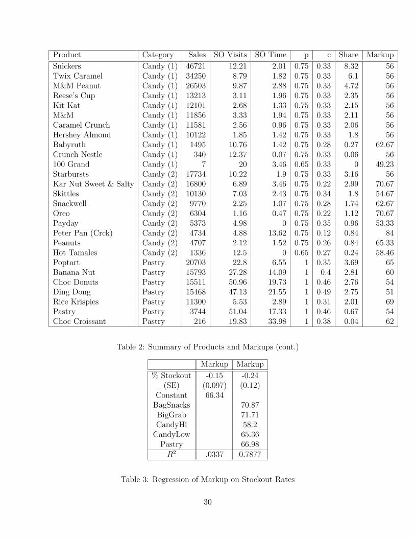
Product Category Sales SO Visits SO Time p c Share Markup

Snickers Candy (1) 46721 12.21 2.01 0.75 0.33 8.32 56Twix Caramel Candy (1) 34250 8.79 1.82 0.75 0.33 6.1 56M&M Peanut Candy (1) 26503 9.87 2.88 0.75 0.33 4.72 56Reese’s Cup Candy (1) 13213 3.11 1.96 0.75 0.33 2.35 56Kit Kat Candy (1) 12101 2.68 1.33 0.75 0.33 2.15 56M&M Candy (1) 11856 3.33 1.94 0.75 0.33 2.11 56Caramel Crunch Candy (1) 11581 2.56 0.96 0.75 0.33 2.06 56Hershey Almond Candy (1) 10122 1.85 1.42 0.75 0.33 1.8 56Babyruth Candy (1) 1495 10.76 1.42 0.75 0.28 0.27 62.67Crunch Nestle Candy (1) 340 12.37 0.07 0.75 0.33 0.06 56100 Grand Candy (1) 7 20 3.46 0.65 0.33 0 49.23Starbursts Candy (2) 17734 10.22 1.9 0.75 0.33 3.16 56Kar Nut Sweet & Salty Candy (2) 16800 6.89 3.46 0.75 0.22 2.99 70.67Skittles Candy (2) 10130 7.03 2.43 0.75 0.34 1.8 54.67Snackwell Candy (2) 9770 2.25 1.07 0.75 0.28 1.74 62.67Oreo Candy (2) 6304 1.16 0.47 0.75 0.22 1.12 70.67Payday Candy (2) 5373 4.98 0 0.75 0.35 0.96 53.33Peter Pan (Crck) Candy (2) 4734 4.88 13.62 0.75 0.12 0.84 84Peanuts Candy (2) 4707 2.12 1.52 0.75 0.26 0.84 65.33Hot Tamales Candy (2) 1336 12.5 0 0.65 0.27 0.24 58.46Poptart Pastry 20703 22.8 6.55 1 0.35 3.69 65Banana Nut Pastry 15793 27.28 14.09 1 0.4 2.81 60Choc Donuts Pastry 15511 50.96 19.73 1 0.46 2.76 54Ding Dong Pastry 15468 47.13 21.55 1 0.49 2.75 51Rice Krispies Pastry 11300 5.53 2.89 1 0.31 2.01 69Pastry Pastry 3744 51.04 17.33 1 0.46 0.67 54Choc Croissant Pastry 216 19.83 33.98 1 0.38 0.04 62

Table 2: Summary of Products and Markups (cont.)

Markup Markup

% Stockout -0.15 -0.24(SE) (0.097) (0.12)

Constant 66.34BagSnacks 70.87BigGrab 71.71CandyHi 58.2

CandyLow 65.36Pastry 66.98

R2 .0337 0.7877

Table 3: Regression of Markup on Stockout Rates

30

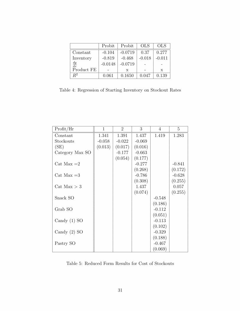
Probit Probit OLS OLS

Constant -0.104 -0.0719 0.37 0.277Inventory -0.819 -0.468 -0.018 -0.011dydx

-0.0148 -0.0719 - -Product FE - x - xR2 0.061 0.1650 0.047 0.139

Table 4: Regression of Starting Inventory on Stockout Rates

Profit/Hr 1 2 3 4 5

Constant 1.341 1.391 1.437 1.419 1.283Stockouts -0.058 -0.022 -0.069(SE) (0.013) (0.017) (0.016)Category Max SO -0.177 -0.663

(0.054) (0.177)Cat Max =2 -0.277 -0.841

(0.268) (0.172)Cat Max =3 -0.786 -0.628

(0.308) (0.255)Cat Max > 3 1.437 0.057

(0.074) (0.255)Snack SO -0.548

(0.186)Grab SO -0.112

(0.051)Candy (1) SO -0.113

(0.102)Candy (2) SO -0.329

(0.188)Pastry SO -0.467

(0.069)

Table 5: Reduced Form Results for Cost of Stockouts

31

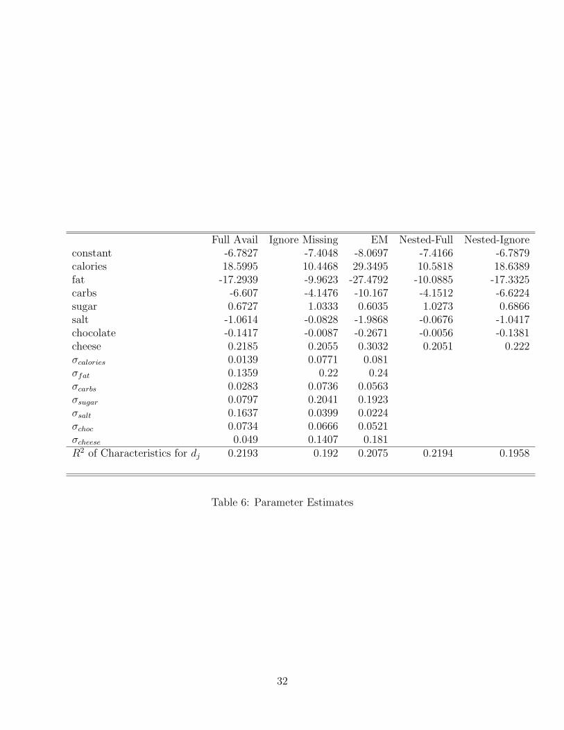
Full Avail Ignore Missing EM Nested-Full Nested-Ignoreconstant -6.7827 -7.4048 -8.0697 -7.4166 -6.7879calories 18.5995 10.4468 29.3495 10.5818 18.6389fat -17.2939 -9.9623 -27.4792 -10.0885 -17.3325carbs -6.607 -4.1476 -10.167 -4.1512 -6.6224sugar 0.6727 1.0333 0.6035 1.0273 0.6866salt -1.0614 -0.0828 -1.9868 -0.0676 -1.0417chocolate -0.1417 -0.0087 -0.2671 -0.0056 -0.1381cheese 0.2185 0.2055 0.3032 0.2051 0.222σcalories 0.0139 0.0771 0.081σfat 0.1359 0.22 0.24σcarbs 0.0283 0.0736 0.0563σsugar 0.0797 0.2041 0.1923σsalt 0.1637 0.0399 0.0224σchoc 0.0734 0.0666 0.0521σcheese 0.049 0.1407 0.181R2 of Characteristics for dj 0.2193 0.192 0.2075 0.2194 0.1958

Table 6: Parameter Estimates

32

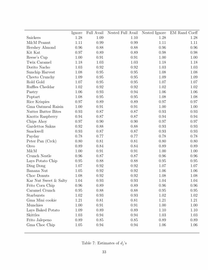
Ignore Full Avail Nested Full Avail Nested Ignore EM Rand CoeffSnickers 1.28 1.09 1.10 1.28 1.28M&M Peanut 1.11 0.99 0.99 1.11 1.11Hershey Almond 0.96 0.88 0.88 0.96 0.96Kit Kat 0.97 0.89 0.89 0.98 0.98Reese’s Cup 1.00 0.91 0.91 1.00 1.00Twix Caramel 1.18 1.03 1.03 1.18 1.18Dorito Nacho 1.03 0.92 0.92 1.03 1.03Sunchip Harvest 1.08 0.95 0.95 1.08 1.08Cheeto Crunchy 1.09 0.95 0.95 1.09 1.09Rold Gold 1.07 0.95 0.95 1.07 1.07Ruffles Cheddar 1.02 0.92 0.92 1.02 1.02Pastry 1.06 0.93 0.94 1.06 1.06Poptart 1.08 0.95 0.95 1.08 1.08Rice Krispies 0.97 0.89 0.89 0.97 0.97Gma Oatmeal Raisin 1.00 0.91 0.91 1.00 1.00Nutter Butter Bites 0.93 0.87 0.87 0.93 0.93Knotts Raspberry 0.94 0.87 0.87 0.94 0.94Chips Ahoy 0.97 0.90 0.90 0.97 0.97Gardettos Snkns 0.92 0.88 0.88 0.93 0.93Snackwell 0.93 0.87 0.87 0.93 0.93Payday 0.78 0.77 0.77 0.78 0.78Peter Pan (Crck) 0.80 0.81 0.81 0.80 0.80Oreo 0.89 0.84 0.84 0.89 0.89M&M 1.00 0.91 0.91 1.00 1.00Crunch Nestle 0.96 0.87 0.87 0.96 0.96Lays Potato Chip 0.95 0.88 0.88 0.95 0.95Ding Dong 1.07 0.92 0.92 1.07 1.07Banana Nut 1.05 0.92 0.92 1.06 1.06Choc Donuts 1.08 0.92 0.92 1.08 1.08Kar Nut Sweet & Salty 1.04 0.93 0.93 1.04 1.04Frito Corn Chip 0.96 0.89 0.89 0.96 0.96Caramel Crunch 0.95 0.88 0.88 0.95 0.95Starbursts 1.02 0.93 0.93 1.02 1.02Gma Mini cookie 1.21 0.81 0.81 1.21 1.21Munchies 1.00 0.91 0.91 1.00 1.00Lays Baked Potato 1.09 0.89 0.89 1.10 1.10Skittles 1.03 0.94 0.94 1.03 1.03Frito Jalepeno 0.89 0.85 0.85 0.89 0.89Gma Choc Chip 1.05 0.94 0.94 1.06 1.06

Table 7: Estimates of dj’s

33

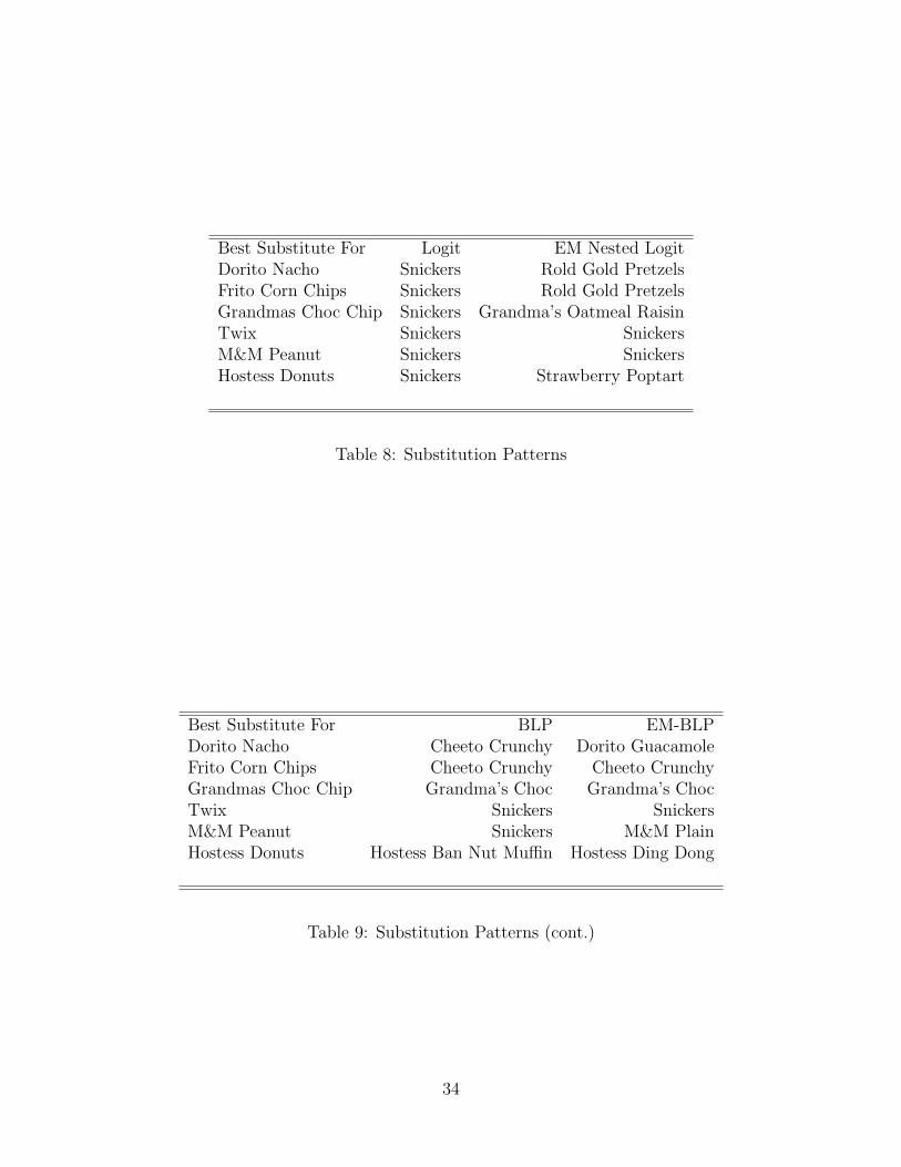
Best Substitute For Logit EM Nested LogitDorito Nacho Snickers Rold Gold PretzelsFrito Corn Chips Snickers Rold Gold PretzelsGrandmas Choc Chip Snickers Grandma’s Oatmeal RaisinTwix Snickers SnickersM&M Peanut Snickers SnickersHostess Donuts Snickers Strawberry Poptart

Table 8: Substitution Patterns

Best Substitute For BLP EM-BLPDorito Nacho Cheeto Crunchy Dorito GuacamoleFrito Corn Chips Cheeto Crunchy Cheeto CrunchyGrandmas Choc Chip Grandma’s Choc Grandma’s ChocTwix Snickers SnickersM&M Peanut Snickers M&M PlainHostess Donuts Hostess Ban Nut Muffin Hostess Ding Dong

Table 9: Substitution Patterns (cont.)

34

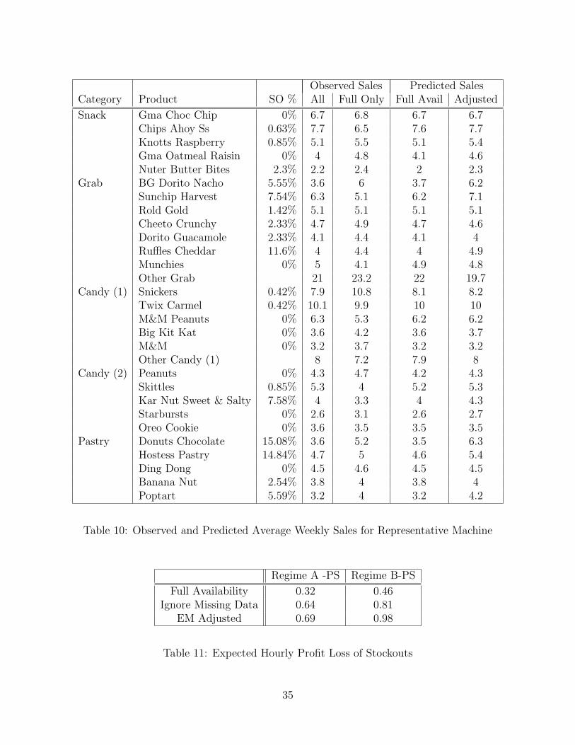
Observed Sales Predicted SalesCategory Product SO % All Full Only Full Avail Adjusted

Snack Gma Choc Chip 0% 6.7 6.8 6.7 6.7Chips Ahoy Ss 0.63% 7.7 6.5 7.6 7.7Knotts Raspberry 0.85% 5.1 5.5 5.1 5.4Gma Oatmeal Raisin 0% 4 4.8 4.1 4.6Nuter Butter Bites 2.3% 2.2 2.4 2 2.3

Grab BG Dorito Nacho 5.55% 3.6 6 3.7 6.2Sunchip Harvest 7.54% 6.3 5.1 6.2 7.1Rold Gold 1.42% 5.1 5.1 5.1 5.1Cheeto Crunchy 2.33% 4.7 4.9 4.7 4.6Dorito Guacamole 2.33% 4.1 4.4 4.1 4Ruffles Cheddar 11.6% 4 4.4 4 4.9Munchies 0% 5 4.1 4.9 4.8Other Grab 21 23.2 22 19.7

Candy (1) Snickers 0.42% 7.9 10.8 8.1 8.2Twix Carmel 0.42% 10.1 9.9 10 10M&M Peanuts 0% 6.3 5.3 6.2 6.2Big Kit Kat 0% 3.6 4.2 3.6 3.7M&M 0% 3.2 3.7 3.2 3.2Other Candy (1) 8 7.2 7.9 8

Candy (2) Peanuts 0% 4.3 4.7 4.2 4.3Skittles 0.85% 5.3 4 5.2 5.3Kar Nut Sweet & Salty 7.58% 4 3.3 4 4.3Starbursts 0% 2.6 3.1 2.6 2.7Oreo Cookie 0% 3.6 3.5 3.5 3.5

Pastry Donuts Chocolate 15.08% 3.6 5.2 3.5 6.3Hostess Pastry 14.84% 4.7 5 4.6 5.4Ding Dong 0% 4.5 4.6 4.5 4.5Banana Nut 2.54% 3.8 4 3.8 4Poptart 5.59% 3.2 4 3.2 4.2

Table 10: Observed and Predicted Average Weekly Sales for Representative Machine

Regime A -PS Regime B-PS

Full Availability 0.32 0.46Ignore Missing Data 0.64 0.81

EM Adjusted 0.69 0.98

Table 11: Expected Hourly Profit Loss of Stockouts

35

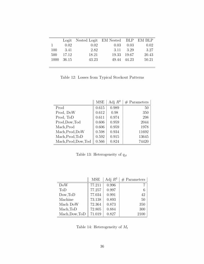
Logit Nested Logit EM Nested BLP EM BLP1 0.02 0.02 0.03 0.03 0.02100 3.41 2.82 3.11 3.29 3.27500 17.12 18.21 19.33 19.67 20.431000 36.15 43.23 49.44 44.23 50.21

Table 12: Losses from Typical Stockout Patterns

MSE Adj R2 # Parameters

Prod 0.615 0.989 50Prod, DoW 0.612 0.98 350Prod, ToD 0.611 0.974 298Prod,Dow,Tod 0.606 0.959 2044Mach,Prod 0.606 0.959 1978Mach,Prod,DoW 0.598 0.934 11692Mach,Prod,ToD 0.592 0.915 13645Mach,Prod,Dow,Tod 0.566 0.824 74420

Table 13: Heterogeneity of qjt

MSE Adj R2 # Parameters

DoW 77.211 0.996 7ToD 77.257 0.997 6Dow,ToD 77.034 0.991 42Machine 73.138 0.893 50Mach DoW 72.364 0.873 350Mach,ToD 72.805 0.884 300Mach,Dow,ToD 71.019 0.827 2100

Table 14: Heterogeneity of Mt

36

References

Aguirregabiria, V. (1999): “The Dynamics of Markups and Inventories in Reatailing

Firms,” Review of Eocnomic Studies, 66, 278–308.

Anupindi, R., M. Dada, and S. Gupta (1998): “Estimation of Consumer Demand with

Stock-Out Based Substitution: An Application to Vending Machine Products,” Marketing

Science, 17(4), 406–423.

Athey, S., and G. Imbens (2006): “Discrete Choice Models with Multiple Unobserved

Choice Characteristics,” .

Berry, S. (1992): “An Esitmation of a Model of Entry in the Airline Industry,” Economet-

rica, (60), 889–917.

(1994): “Estimating discrete-choice models of product differentiation,” RAND

Journal of Economics, 25(2), 242–261.

Berry, S., J. Levinsohn, and A. Pakes (1995): “Automobile Prices in Market Equilib-

rium,” Econometrica, 63(4), 841–890.

(2004): “Automobile Prices in Market Equilibrium,” Journal of Political Economy,

112(1), 68–105.

Dempster, A. P., N. M. Laird, and D. B. Rubin (1977): “Maximum Likelihood from

Incomplete Data via the EM Algorithm,” Journal of the Royal Statistical Society, 39(1),

1–38.

Draganska, M., and D. Jain (2004): “A Likelihood Appraoch to Estimating Market

Equilibrium Models,” Management Science, 50(5), 605–616.

Hadley, G., and T. Whitman (1963): Analysis of Inventory Systems. Prentice Hall.

Hartley, H. (1958): “Maximum Likelihood from Incomplete Data,” Biometrics, 14(2),

174–194.

Liu, C., and D. B. Rubin (1994): “The ECME algorithm: A simple extension of EM and

ECM with faster monotone convergence,” Biometrika, 81, 633–648.

37

Matzkin, R. (1992): “Nonparametric and Distribution-Free Estimation of Binary Thresh-

old Crossing Models,” Econometrica, 60(2), 239–270.

McFadden, D., and K. Train (2000): “Mixed MNL Models for Discrete Response,”

Journal of Applied Econometrics, 15, 447–470.

Musalem, A., E. T. Bradlow, and J. S. Raju (2006): “Bayesian Estimation of

Random-Coefficients Chocie Models Using Aggregate Data,” .

Nevo, A. (2000): “Mergers with differentiated products: the case of the ready-to-eat cereal

industry,” RAND Journal of Economics, 31(3), 395–421.

(2001): “Measuring Market Power in the Ready-to-Eat Cereal Industry,” Econo-

metrica, 69, 307–342.

Nevo, A., and I. Hendel (2007a): “Measuring Implications of Sales and Consumer In-

ventory Behavior,” Econometrica.

(2007b): “Sales and Consumer Inventory,” The RAND Journal of Economics.

Nevo, A., and C. Wolfram (2002): “Why Do Manufacturers Issue Coupons? An Em-

pirical Analysis of Breakfast Cereals,” The RAND Journal of Economics, 33(2), 319–339.

Petrin, A. (2002): “Quantifying the Benefits of New Products: The Case of the Minivan,”

Journal of Political Economy, 110(4), 705–729.

Rubin, D. B. (1976): “Inference and Missing Data,” Biometrika, 63, 581–592.

38