Embed Size (px)
Citation preview

Charlotte Karlshøj Madsen (s042539)Kristín Ósk Þórðardóttir (s053258)
Demand as FrequencyControlled Reserve
Advanced Modeling of Aggregating FrequencyResponsive Loads in Power System DynamicSimulation
Bachelor’s Thesis, Summer 2007


Charlotte Karlshøj Madsen (s042539)Kristín Ósk Þórðardóttir (s053258)
Demand as FrequencyControlled Reserve
Advanced Modeling of Aggregating FrequencyResponsive Loads in Power System DynamicSimulation
Bachelor’s Thesis, Summer 2007


Demand as Frequency Controlled Reserve, Advanced Modeling ofAggregating Frequency Responsive Loads in Power System DynamicSimulation.
This report is made by: Charlotte Karlshøj Madsen (s042539)Kristín Ósk Þórðardóttir (s053258)
Supervisors: Jacob ØstergaardZhao Xu
Ørsted • DTUCentre for Electric Technology (CET)Technical University of DenmarkElektrovej 325DK-2800 Kgs. LyngbyDenmark
www.oersted.dtu.dk/cetTel: (+45) 45 25 35 00Fax: (+45) 45 88 61 11E-mail: [email protected]
Date of submission: 29th June 20007Class: 1 (Public)
Edition: 1st
Remarks: This report has been submitted as a step in fulfilling thedemands for receiving the degree of Bachelor of Sci-ence in Engineering from the Technical University ofDenmark. The report represents 15 ECTS points.
Copyright 2007 c© Charlotte K. Madsen & Kristín Ó. Þórðardóttir


Abstract
This project examines the behavior of frequency controlled loads (FCLs) whenaccumulated on a grid, and has the aim to estimate a transfer function (TF),that describes these loads. The grid is the Danish electrical grid and all specifi-cations relate to it.
The basis of the modeling is dynamic simulations in the power system programDIgSilent Power Factory (PF) of a model built with heaters as FCLs. These ag-gregating loads simulate the behavior very closely and the model has been builtas a part of a larger project; PSO Project on Demand as Frequency ControlledReserve in which this project is also a part.
During this project, we wish to use system identification method to derive theTF. The foundation for the modeling is System Identification Tool (SIT) in MAT-LAB and the possibilities and limitations from this affects the model.
The FCL create the dependency between the frequency and the demand that isthe main interest in this project. To work as a reserve either by lowering thetotal demand or by gaining time for other reserve to cut in, the demand has toresponse by falling when the frequency falls.
The TFs derived do display the wanted behavior also incorporated in the orig-inal system in PF. The level of detail is not as great as the PF model but thetendency is caught by the TFs. he order spans from third to fifth order but themodels might need a much higher order for the TFs to become more accurate. Afurther investigation in PF with a different dependency between the signals re-vealed a very complex behavior of the FCLs. This is most likely better describedwith a more complex model than the TFs derived here.
The limitations of SIT play a significant part in the general method in thisproject and the entire method needs revisioning for further investigations. Whentransforming the derived models in both form and time the purpose needs to beassociated with the electrical behavior of the models since a trade-off in proper-ties is inevitable.
I

Resume
Dette projekt undersøger akkumulerede frekvenskontrollerede belastningers(FCL) opførsel på et netværk og har til formål at udlede en overførselsfunk-tion (TF) som beskriver disse belastninger. Netværket er det danske elektriskenet og alle specifikationer relaterer til dette.
Basis for modelleringen er dynamiske simuleringer i energiforsyningsprogram-met DIgSilent Power Factory (PF) af en model opbygget af varmeapparater somFCL. Disse akkumulerede belastninger simulerer den elektriske opførsel medstor nøjagtighed og modellen er er bygget som en del af et større projekt; PSOProject on Demand as Frequency Controlled Reserve (Projekt vedrørende for-brug som frekvenskontrolleret reserve) i hvilket dette projekt også indgår.
I dette projekt ønsker vi at bruge system identifikationsmetoden til at udledeen overførselsfunktion. Grundlaget for modelleringen er System IdentificationTool (SIT) i MATLAB og mulighederne og begrænsningerne for dette påvirkermodellen.
Afhængigheden mellem forbrug og frekvens skabt a FCL er hovedinteressen idette projekt. For at virke som reserve enten ved at formindske forbruget ellerved at forsinke forbruget, og vinde tid til at andre reserver kan koble ind, skaldet falde når frekvensen falder.
De udledte TF udviser den ønskede opførsel også i samspil med det oprindeligsystem i PF. Graden af detaljer er ikke så høj som for PF modellen men ten-densen vises tydeligt af TF. Graden af TF spænder fra tredje til femte men mod-ellerne bør sandsynligvis være af en meget højere orden for at blive mere detal-jerede. En nærmere undersøgelse i PF, med en anden afhængighed signalerneimellem, viste at FCL har en meget kompleks opførsel som højst sandsynligtbeskrives bedre med en mere avanceret model end de her udledte.
Begrænsningerne i SIT spiller en betydelig rolle i den generelle metode brugti dette projekt, og denne metode bør revideres i tilfælde af yderligere under-søgelser. Når de udledte modeller transformeres i form og tid må formåletholdes for øje sammen med de elektriske egenskaber for modellen da en vek-selvirkning mellem egenskaber er uundgåelig.
II

Contents
Abstract I
Resume II
Preface 1Background . . . . . . . . . . . . . . . . . . . . . . . . . . . . . . . 1
The context . . . . . . . . . . . . . . . . . . . . . . . . . . . . 1Problem Formulation . . . . . . . . . . . . . . . . . . . . . . . . . . 2Method . . . . . . . . . . . . . . . . . . . . . . . . . . . . . . . . . . 2
1 The Power Factory System 51.1 Interaction in the Model . . . . . . . . . . . . . . . . . . . . . . . . 5
1.1.1 Special Feature of the System . . . . . . . . . . . . . . . . . 51.2 The Theory Behind the System . . . . . . . . . . . . . . . . . . . . 6
1.2.1 The Heater Block . . . . . . . . . . . . . . . . . . . . . . . . 61.2.2 Strengths and Weaknesses . . . . . . . . . . . . . . . . . . . 7
1.3 Use of the System . . . . . . . . . . . . . . . . . . . . . . . . . . . . 81.3.1 The Main Simulation . . . . . . . . . . . . . . . . . . . . . . 81.3.2 The Datasets . . . . . . . . . . . . . . . . . . . . . . . . . . . 8
2 System Identification 112.1 Theory on System Identification . . . . . . . . . . . . . . . . . . . . 112.2 The Process of System Identification . . . . . . . . . . . . . . . . . 11
2.2.1 The System Identification Loop . . . . . . . . . . . . . . . . 12
3 Estimations in SIT 133.1 Options and Preparing . . . . . . . . . . . . . . . . . . . . . . . . . 13
3.1.1 Basic Equations and Options . . . . . . . . . . . . . . . . . 133.1.2 Preprocessing the Data . . . . . . . . . . . . . . . . . . . . . 14
3.2 Performing Estimations . . . . . . . . . . . . . . . . . . . . . . . . 153.2.1 The set of Main Estimations . . . . . . . . . . . . . . . . . . 153.2.2 Estimations on Different Dataset . . . . . . . . . . . . . . . 17
4 Evaluating the Models 194.1 Theory of Regulation Technique . . . . . . . . . . . . . . . . . . . . 19
4.1.1 Zeros and Poles . . . . . . . . . . . . . . . . . . . . . . . . . 19
III

4.1.2 Step and Impulse Responses . . . . . . . . . . . . . . . . . . 194.2 Using the SIT Tools . . . . . . . . . . . . . . . . . . . . . . . . . . . 20
4.2.1 Significance of Correlation . . . . . . . . . . . . . . . . . . . 204.2.2 Model Failure . . . . . . . . . . . . . . . . . . . . . . . . . . 204.2.3 Model Evaluation . . . . . . . . . . . . . . . . . . . . . . . . 20
4.3 Comparison to Other Datasets . . . . . . . . . . . . . . . . . . . . 214.4 Exporting the Models . . . . . . . . . . . . . . . . . . . . . . . . . . 22
5 The Transfer Function 235.1 Deriving TF From SIT Polynomials . . . . . . . . . . . . . . . . . . 23
5.1.1 From Polynomials to TF . . . . . . . . . . . . . . . . . . . . 245.1.2 From Discrete to Continuous Time . . . . . . . . . . . . . . 24
5.2 Analyzing the TF . . . . . . . . . . . . . . . . . . . . . . . . . . . . 265.2.1 Step and Impulse Responses . . . . . . . . . . . . . . . . . . 265.2.2 Bode Plots . . . . . . . . . . . . . . . . . . . . . . . . . . . . 30
5.3 Visualizing the TF in MATLAB Simulink . . . . . . . . . . . . . . . 315.4 Concluding Remarks . . . . . . . . . . . . . . . . . . . . . . . . . . 33
6 TF in Main Case PF 356.1 Preparing new Simulations in PF . . . . . . . . . . . . . . . . . . . 35
6.1.1 Converting to State-Space Form . . . . . . . . . . . . . . . 356.1.2 Creating a PF Macro From the TF . . . . . . . . . . . . . . 36
6.2 First Simulations Experiences . . . . . . . . . . . . . . . . . . . . . 366.2.1 Adapting the TF . . . . . . . . . . . . . . . . . . . . . . . . . 37
6.3 The Behavior in Main Case . . . . . . . . . . . . . . . . . . . . . . 386.3.1 The Event Reaction . . . . . . . . . . . . . . . . . . . . . . . 406.3.2 Initial Oscillation . . . . . . . . . . . . . . . . . . . . . . . . 416.3.3 Comparison . . . . . . . . . . . . . . . . . . . . . . . . . . . 43
6.4 Concluding Remarks . . . . . . . . . . . . . . . . . . . . . . . . . . 43
7 Step Case 457.1 Data From PF . . . . . . . . . . . . . . . . . . . . . . . . . . . . . . 457.2 Estimating a Model in SIT . . . . . . . . . . . . . . . . . . . . . . . 457.3 Deriving the TF in MATLAB . . . . . . . . . . . . . . . . . . . . . . 477.4 Simulating in PF . . . . . . . . . . . . . . . . . . . . . . . . . . . . 497.5 Concluding Remarks . . . . . . . . . . . . . . . . . . . . . . . . . . 49
8 Conclusion 51
Bibliography 53
IV
Appendix 55
A Flowcharts 56A.1 For the Entire Project . . . . . . . . . . . . . . . . . . . . . . . . . . 56A.2 For using the SIT in details . . . . . . . . . . . . . . . . . . . . . . 57
B “How To” in SIT 59B.1 Loading the Data . . . . . . . . . . . . . . . . . . . . . . . . . . . . 59B.2 Creating the Datasets . . . . . . . . . . . . . . . . . . . . . . . . . 59
B.2.1 Starting the SIT Tool . . . . . . . . . . . . . . . . . . . . . . 60B.2.2 Importing the Data . . . . . . . . . . . . . . . . . . . . . . . 60B.2.3 Working With one Dataset . . . . . . . . . . . . . . . . . . . 61
B.3 Preparing the Data . . . . . . . . . . . . . . . . . . . . . . . . . . . 61B.4 Estimations . . . . . . . . . . . . . . . . . . . . . . . . . . . . . . . 63
B.4.1 Estimation Panel and Options . . . . . . . . . . . . . . . . . 63B.4.2 Eliminating Poor Estimations Using Model Views . . . . . 64B.4.3 Examining Models in LTI Viewer . . . . . . . . . . . . . . . 67
B.5 Validating Models . . . . . . . . . . . . . . . . . . . . . . . . . . . . 68B.5.1 Working With Several Datasets . . . . . . . . . . . . . . . . 68
B.6 SIT Summary . . . . . . . . . . . . . . . . . . . . . . . . . . . . . . 70
C Illustrations From SIT 71
D Model in Simulink 79
E More Possibilities in PF 81E.1 Main Case . . . . . . . . . . . . . . . . . . . . . . . . . . . . . . . . 81E.2 Step Case . . . . . . . . . . . . . . . . . . . . . . . . . . . . . . . . . 83
V
List of Figures
1.2.1 Block Diagram, Main Case . . . . . . . . . . . . . . . . . . . . . . 71.3.1 Main Result From PF . . . . . . . . . . . . . . . . . . . . . . . . . 9
2.1.1 System Identification Model . . . . . . . . . . . . . . . . . . . . . . 112.2.1 System Identification Flowchart . . . . . . . . . . . . . . . . . . . 12
3.1.1 Input and Output Signals . . . . . . . . . . . . . . . . . . . . . . . 143.2.1 Various Models Output . . . . . . . . . . . . . . . . . . . . . . . . . 163.2.2 Model Output Zoom . . . . . . . . . . . . . . . . . . . . . . . . . . 163.2.3 Initial Model Output Zoom . . . . . . . . . . . . . . . . . . . . . . 173.2.4 ARX Models Output . . . . . . . . . . . . . . . . . . . . . . . . . . 183.2.5 New Models Output Zoom . . . . . . . . . . . . . . . . . . . . . . . 18
4.3.1 Model Output Start . . . . . . . . . . . . . . . . . . . . . . . . . . . 22
5.1.1 Bode Plot, Tustin and Zero Order Hold . . . . . . . . . . . . . . . 255.2.1 Step/Impulse Responses, SIT, OE . . . . . . . . . . . . . . . . . . . 275.2.2 Discrete Time Responses, MATLAB, OE . . . . . . . . . . . . . . . 275.2.3 Step/Impulse Responses, SIT, ARX . . . . . . . . . . . . . . . . . . 285.2.4 Discrete Time Responses, MATLAB, ARX . . . . . . . . . . . . . . 285.2.5 Continuous Time Responses, OE . . . . . . . . . . . . . . . . . . . 295.2.6 Continuous Time Responses, ARX . . . . . . . . . . . . . . . . . . 295.2.7 Bode Plot, SIT . . . . . . . . . . . . . . . . . . . . . . . . . . . . . . 305.2.8 Bode Plot, MATLAB . . . . . . . . . . . . . . . . . . . . . . . . . . . 305.3.1 Simulink Model of the TF . . . . . . . . . . . . . . . . . . . . . . . 315.3.2 Power and Frequency From Simulink Model, OE . . . . . . . . . 315.3.3 Power and Frequency From Simulink Model, ARX . . . . . . . . . 325.3.4 OE and ARX Models, SIT . . . . . . . . . . . . . . . . . . . . . . . 32
6.1.1 Macro in PF . . . . . . . . . . . . . . . . . . . . . . . . . . . . . . . 366.2.1 Grid in Power Factory . . . . . . . . . . . . . . . . . . . . . . . . . 376.2.2 Comparison of the Impulse Responses for OE and ARX . . . . . . 396.3.1 Power Demand of OE in PF . . . . . . . . . . . . . . . . . . . . . . 406.3.2 Power Demand of ARX in PF . . . . . . . . . . . . . . . . . . . . . 416.3.3 Overshoot in PF, OE . . . . . . . . . . . . . . . . . . . . . . . . . . 426.3.4 Overshoot in PF, ARX . . . . . . . . . . . . . . . . . . . . . . . . . 42
VI

7.1.1 Block Diagram, Step Case . . . . . . . . . . . . . . . . . . . . . . . 457.1.2 Power and Frequency, PF . . . . . . . . . . . . . . . . . . . . . . . 467.2.1 Stepdata in SIT, Mean Zero . . . . . . . . . . . . . . . . . . . . . . 467.2.2 Best Fit, Step Input . . . . . . . . . . . . . . . . . . . . . . . . . . 477.2.3 Step/Impulse Responses, SIT . . . . . . . . . . . . . . . . . . . . . 487.3.1 Step/Impulse Responses, MATLAB . . . . . . . . . . . . . . . . . . 487.4.1 Power Demand in PF, Step Input . . . . . . . . . . . . . . . . . . . 49
Appendix 55
A.1 Flowchart for the Entire Project . . . . . . . . . . . . . . . . . . . 56A.2 Flowchart for SIT . . . . . . . . . . . . . . . . . . . . . . . . . . . . 57
B.1 SIT Untitled; Main Panel . . . . . . . . . . . . . . . . . . . . . . . 60B.2 Import Data Panel . . . . . . . . . . . . . . . . . . . . . . . . . . . 60B.3 Complete Import Panel . . . . . . . . . . . . . . . . . . . . . . . . . 61B.4 Panel with Mean Dataset . . . . . . . . . . . . . . . . . . . . . . . 62B.5 Frequency Function & Time Plot . . . . . . . . . . . . . . . . . . . 62B.6 Parametric Models Panel . . . . . . . . . . . . . . . . . . . . . . . 63B.7 Panel With Data and Models . . . . . . . . . . . . . . . . . . . . . 64B.8 Data/models Info . . . . . . . . . . . . . . . . . . . . . . . . . . . . 64B.9 Model Output: Demand . . . . . . . . . . . . . . . . . . . . . . . . 65B.10 Residuals, Zeros and Poles . . . . . . . . . . . . . . . . . . . . . . . 65B.11 Frequency Function & Noise Spectrum . . . . . . . . . . . . . . . 66B.12 Transient Response . . . . . . . . . . . . . . . . . . . . . . . . . . . 66B.13 LTI Viewers . . . . . . . . . . . . . . . . . . . . . . . . . . . . . . . 67B.14 Several Datasets . . . . . . . . . . . . . . . . . . . . . . . . . . . . 68B.15 Time Plot; Two Datasets . . . . . . . . . . . . . . . . . . . . . . . . 69B.16 Model Output; New Dataset . . . . . . . . . . . . . . . . . . . . . . 69
C.1 Estimation Various . . . . . . . . . . . . . . . . . . . . . . . . . . 71C.2 Estimations ARX . . . . . . . . . . . . . . . . . . . . . . . . . . . . 71C.3 Power Spectrums . . . . . . . . . . . . . . . . . . . . . . . . . . . . 72C.4 Residuals ARX & ARMAX . . . . . . . . . . . . . . . . . . . . . . . 72C.5 Cross Correlations OE . . . . . . . . . . . . . . . . . . . . . . . . . 73C.6 Frequency Responses . . . . . . . . . . . . . . . . . . . . . . . . . . 73C.7 Poles and Zeros . . . . . . . . . . . . . . . . . . . . . . . . . . . . . 74C.8 Step and Impulse Responses Overall . . . . . . . . . . . . . . . . . 74C.9 Step and Impulse Responses OE . . . . . . . . . . . . . . . . . . . 75C.10 Step and Impulse Responses ARX . . . . . . . . . . . . . . . . . . 75C.11 Sorted Models . . . . . . . . . . . . . . . . . . . . . . . . . . . . . . 76C.12 Models Output & Fit . . . . . . . . . . . . . . . . . . . . . . . . . . 76C.13 All Residuals . . . . . . . . . . . . . . . . . . . . . . . . . . . . . . 77
VII

D.1 Simulink, Temperature Set Points . . . . . . . . . . . . . . . . . . 79D.2 Simulink Model of the PF system . . . . . . . . . . . . . . . . . . . 80
E.1 Simulated Results of OE, PF . . . . . . . . . . . . . . . . . . . . . 81E.2 Simulated Results of ARX, PF . . . . . . . . . . . . . . . . . . . . 82E.3 Block Diagram, Macro . . . . . . . . . . . . . . . . . . . . . . . . . 83E.4 Output ARX521, Loop Re-established . . . . . . . . . . . . . . . . 83
VIII
Preface
Background
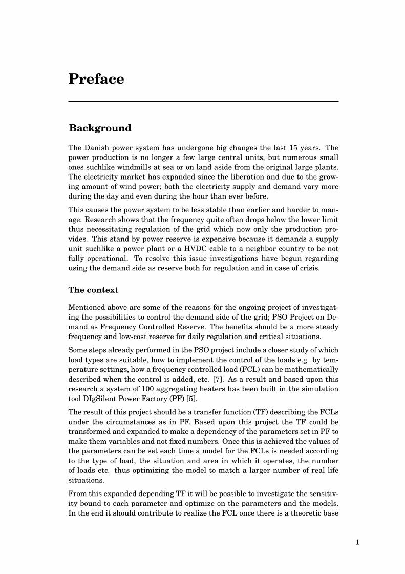
The Danish power system has undergone big changes the last 15 years. Thepower production is no longer a few large central units, but numerous smallones suchlike windmills at sea or on land aside from the original large plants.The electricity market has expanded since the liberation and due to the grow-ing amount of wind power; both the electricity supply and demand vary moreduring the day and even during the hour than ever before.
This causes the power system to be less stable than earlier and harder to man-age. Research shows that the frequency quite often drops below the lower limitthus necessitating regulation of the grid which now only the production pro-vides. This stand by power reserve is expensive because it demands a supplyunit suchlike a power plant or a HVDC cable to a neighbor country to be notfully operational. To resolve this issue investigations have begun regardingusing the demand side as reserve both for regulation and in case of crisis.
The context
Mentioned above are some of the reasons for the ongoing project of investigat-ing the possibilities to control the demand side of the grid; PSO Project on De-mand as Frequency Controlled Reserve. The benefits should be a more steadyfrequency and low-cost reserve for daily regulation and critical situations.
Some steps already performed in the PSO project include a closer study of whichload types are suitable, how to implement the control of the loads e.g. by tem-perature settings, how a frequency controlled load (FCL) can be mathematicallydescribed when the control is added, etc. [7]. As a result and based upon thisresearch a system of 100 aggregating heaters has been built in the simulationtool DIgSilent Power Factory (PF) [5].
The result of this project should be a transfer function (TF) describing the FCLsunder the circumstances as in PF. Based upon this project the TF could betransformed and expanded to make a dependency of the parameters set in PF tomake them variables and not fixed numbers. Once this is achieved the values ofthe parameters can be set each time a model for the FCLs is needed accordingto the type of load, the situation and area in which it operates, the numberof loads etc. thus optimizing the model to match a larger number of real lifesituations.
From this expanded depending TF it will be possible to investigate the sensitiv-ity bound to each parameter and optimize on the parameters and the models.In the end it should contribute to realize the FCL once there is a theoretic base
1

Preface
to choose the kind of load, the best way to control them, and where and when touse them. Not to mention if the effect of this enterprise will be great enough tofind financial support.
Problem Formulation
The aim of this project is deriving a transfer function that describes severalaggregating frequency controlled loads. The transfer function should representthe behavior of all the loads when operating connected to the Danish powersystem. The basis is a system build in Power Factory from which simulateddata is extracted to built a model. After reconfiguring the TF model into itsfinal state, a comparison to the initial data will show its accuracy. Below is theconsideration this project aims to clarify.
• Is it possible to describe the behavior of the aggregated loads with a the-oretical expression such as a transfer function within a reasonable devia-tion?
• How can this transfer function be derived using MATLAB?
• Considering the context of the TF model, how well does it describe theloads?
• Which information does this TF provide about the aggregated loads in amore general matter than what the system shows in simulations?
• Can the TF be put into use combined with other system elements presentin the grid such as replacing the heater block in the PF system?
Method
Our approach to derive the TF requires the use of a few tools and is stagedroughly as following; the first step is extracting the data from PF into a univer-sal form such as a list of numbers. Next we wish to use the System Identifica-tion Toolbox (SIT) in MATLAB to make a model from the PF data, and also byusing SIT we select a small number of models to investigate further.
From the SIT models we derive TFs using MATLAB. These TFs should be bothvalidated and investigated to prove their fit and describe their behavior, andthat is the third step. Last step is replacing the load block in the PF systemwith the TF to compare it with the initial data from the first simulation thusobserving the fit of the TF when combined with the rest of the system.
The system in PF is already provided from [5] and most of the modeling isperformed in SIT. For this part see a detailed “How To” guide in appendix Bthat allows a repetition of deriving the SIT models and describes the actionsdone in SIT to complete this project.
The figure on page 3 shows the rough stages of the project (yellow boxes) and
2 Demand as Frequency Controlled Reserve //Problem Formulation
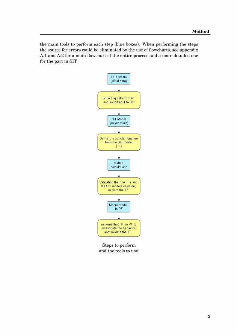
Method
the main tools to perform each step (blue boxes). When performing the stepsthe source for errors could be eliminated by the use of flowcharts, see appendixA.1 and A.2 for a main flowchart of the entire process and a more detailed onefor the part in SIT.
Steps to performand the tools to use
3


Chapter 1The Power Factory System
This chapter contains the information about the Power Factory (PF) systems,from which this project receives its basic data. The two models are referred toas the Main Case and the Step Case see [5] and this chapter covers the MainCase. The system contains theoretical room heaters that are frequency con-trolled loads (FCLs) and simulate the behavior by a numerical process. Amongthe output of these simulations are the time depending frequency and powerconsumption (demand) of the heaters, which is the data of interest for thisproject. These signals are collected in datasets which is then exported for fur-ther use in MATLAB.
1.1 Interaction in the Model
Investigating the behavior of FCL is difficult because of the great dependenciesamong the signals. The frequency controls the temperature settings, and bythat the current power consumption of the heaters, thus equally the power con-sumption all in all. The frequency is depending on the grid power in the waythat it is depending on the state of the entire net. The heaters are controlled bytheir settings, thus by the surrounding temperature which depends on the heatloss i.e. by time. See page 7, figure 1.2.1 for a schematic view.
This means that even though the heaters turn off right away and have a positiveeffect on the demand and the frequency, they will turn on again all together ina bunch, rising the demand noticeably and lowering the frequency once again.This lowers the temperature band making another bunch of heaters turn offprematurely, which then again turns on in a bunch later on. The bunching upof the heaters will fade out, making their demand steady allowing the frequencyto find a steady state as well. This complex behavior is most easily investigatedby making a model incorporating the knowledge already codified, and then runsimulations to see if the considerations match the estimations.
1.1.1 Special Feature of the System
The main purpose of the system is simulating the FCL’s behavior. The simula-tions are numerical and contain information about the entire 100 heaters; thefrequency and the power both consumed by the FCL and in total, the temper-ature settings both the lower and the upper limit, and the 100 different roomtemperatures, all signals according to the time.
The distinction between ordinary systems and this models is that the frequencyturns the heaters on and off by controlling the temperature settings thus mak-
5

The Power Factory System
ing the heaters turn off right when needed, and turn on again at a later pointwhen the falling temperature in the room makes it necessary. The effect of let-ting the frequency control the temperature settings shows in a longer period oftime and not just when the heaters initially turns off. The demand of the groupof heaters, turning off and on for a while, will effect the system until steadystate is reached again. This is a special feature of the system, and a result ofthe heaters being frequency controlled.
1.2 The Theory Behind the System
In PF some standard elements are incorporated and model the behavior of such,but for the FCL heaters a special block has been built with mathematics. Thissection describes the theory behind this customized block of heaters and that ofthe entire system in short.
1.2.1 The Heater Block
The system block is built of 100 identical heaters in identical rooms, or at leastthe heating periods are equally long demanding equally amounts of energy,equally with the cooling down. The heaters have the same demand 1 MW whenturned on, and all in all this gives them the accumulated mean demand atPss = 20 MW when in steady state. The physical heaters and the rooms arenecessarily as described, because the heating up and cooling down follows thesame differential equation:
CdT
dt+ G(T − Ta) + Pwater = w P (1.2.1)
Where C is the heat capacity of the heating mass, G is the thermal conductancebetween the heated mass with the temperature T (indoor) and non-heated masswith temperature Ta (outdoor). The P is the heat power (i.e. the demand, notconsidering the ratio between electrical demand and power used for heating),Pwater is the loss and w determines the state of the heater; w = 1 when theheater is on, w = 0 when off. This parameter is controlled by the temperaturesettings cf. equation (1.2.2).
In the simulation performed in this project, the parameters have been fixed soC = 10 J/◦C, G = 0.02 W/◦C (the thickness of the walls is incorporated in thevalue of G), Ta = 15◦C and a constant loss of Pwater = 0.1 W. Furthermorea small delay of Tmdelay = 0.4 s models the time for measuring the frequencyand regulating the temperature settings Thigh and Tlow that correspond to thepresent frequency f :
Thigh = Ttop + kf (f − f0) and Tlow = Tbot + kf (f − f0) (1.2.2)
Where the temperatures Ttop and Tbot are the deviation band with a width of 4◦Caround the fixed temperature Tset depending on the wanted room temperature.
6 Demand as Frequency Controlled Reserve // 1.2 The Theory Behind the System

1.2 The Theory Behind the System
In Power Factory Tset = 20◦C making Tbot = 18◦C and Ttop = 22◦C. The standardfrequency is f0 = 50Hz and the relation constant is kf = 15.
if T > Thigh then w = 0
if T < Tlow then w = 1 (1.2.3)if Tlow ≤ T ≤ Thigh then w = w
Thus the variables Thigh and Tlow only depend on the frequency f , and they con-trol the parameter w together with the temperature T , which again controls thedemand P . The way from f to P is first through (1.2.2), recalling T , switchingthe w and running (1.2.1). This gives new values to T , P and through the gridP affects the frequency and the cycle repeats.
Figure 1.2.1: Block diagram for the PF system
A more detailed Simulink model has been made in MATLAB see appendix Dfrom page 79, where equations (1.2.1) through (1.2.3) are used to built themodel.
1.2.2 Strengths and Weaknesses
As all models the PF system has strengths and weaknesses, and some areroughly stated here. The program is a very advanced tool and performs strongcalculations, but still it is a simulation tool and does not necessarily match thereality. Also, the construction of the heaters can vary from reality, and somesuggestions to add in the future are given here.
The heaters and the rooms are all the same, and has not all parameters takinginto consideration; especially the losses from human behavior suchlike openingdoors (traffic in the rooms) or windows can be a major liability, but also theweather (day long sunshine) and the heat from people and equipment could beincluded. The parameters C and G could be given to each heater from some sortof investigation or statistic spread, to optimize their values.
Still the system describes the reality under vast periods and is able to connectthe signals in the complex manor as described earlier in section 1.1 on page 5.
7

The Power Factory System
This gives the possibility to examine the accumulated behavior when a lot ofFCLs are connected to a grid that also supplies ordinary loads and matches thecondition of the real electrical network closely.
1.3 Use of the System
By running a simulation it is possible to withdraw data from the system anduse elsewhere. The simulation can give an overwhelming amount of data undervarious conditions, so the challenge is picking out a descriptive dataset. Fromthe electrical network point of view the interesting information is how great thedemand P responses, depending on the frequency f , so to create the datasetsthe system is manipulated by a load event to make the frequency drop.
1.3.1 The Main Simulation
The data contracted from the system (Main Case) is a simulation over a longperiod, since both power and frequency oscillate before reaching steady state.At a point the system is loaded with an extra general load, which makes thefrequency drop thus the heaters demand as well, simulating the case of interest.The system stabilizes the frequency and demand at a new level, the result isdepicted in figure 1.3.1 on the next page. As the figure shows, the frequencyand the demand experience initial oscillation for 400-500 seconds. When 1,000seconds have past a load of 100 MW is switched on, making the total power rise(green curve) and the frequency fall. The grid is now in a new state, and P
changes as f changes. The steady state is almost but not totally reached 1,000seconds later and the accumulated demand in steady state after the event Psse
becomes approx. 16 MW while the frequency settles at fsse = 49.89 Hz.
1.3.2 The Datasets
All in all the simulation results in 200,000 measurements, and these are splitin two datasets at the event time te = 1, 000 i.e. when the demand and the totalpower are no longer the same; Pgrid = P + 100.
The two datasets are stored in PFdata.txt and start.txt, also referred to as eventdata(set) and start data. The estimations performed and described in the fol-lowing have the event data as basis, but it is important that an estimationmodel also reacts the proper way to begin with. This consideration is reactedupon ahead in section 4.3 on page 21.
8 Demand as Frequency Controlled Reserve // 1.3 Use of the System

1.3 Use of the System
Figure 1.3.1: The main result of a simulation in PF lasting 2,000 seconds. The redlines are those of interest in this project. The green line on the lower window showsthe total power on the grid, and where it rises is the switch event
9


Chapter 2System Identification
This chapter contains basic theory behind the method used throughout thisproject, that is System Identification. Built inside MATLAB is a program calledSystem Identification Tool, referred to as SIT in this project. This program isvery useful in the procedure of finding a model describing the system mentionedin chapter 1.
2.1 Theory on System Identification
The idea behind system identification is to use experimental data, i.e. a mea-sured input signal, u(t) and a measured output signal, y(t) to obtain a model ofa given dynamic system. In general there are inputs to real systems, which can-not be measured or controlled and such inputs affect the output of the systemand are called disturbances or noise, e(t).
Figure 2.1.1: A model of a measured input u(t), un-measured noise e(t) and a measured output y(t).
For linear models, the general symbolic model description is given by:
y(t) = H(q)u(t) + G(q)e(t) (2.1.1)
Where, H is an operator describing the system dynamics i.e. a TF between u(t)and y(t). In system identification H can by a number of variety of mathematicalforms. G is an operator which describes the output disturbance.
2.2 The Process of System Identification
In the process of constructing a model from any data the following entities needto be considered:
1. The data set. The input and output data should be carefully chosen inrespect to which signals to measure and when to measure them e.g. aftera load event has happened, to study the response of the system.
11
System Identification
2. The model structure. As described in the next chapter a number of candi-date models can be obtained by specifying within which collection of mod-els estimations are suitable. This process is very important and perhapsthe most difficult one.
3. Determining the best model. This process concerns the model qualitybased on the performance of the model when in attempt to resemble themeasured data. See section 4.2 on page 20.
When using System Identification we need to keep in mind that models cannever be accepted as a true and final description of a system, but rather a gooddescription of certain aspects that interest us. This is explained when evaluat-ing the models in chapter 4.
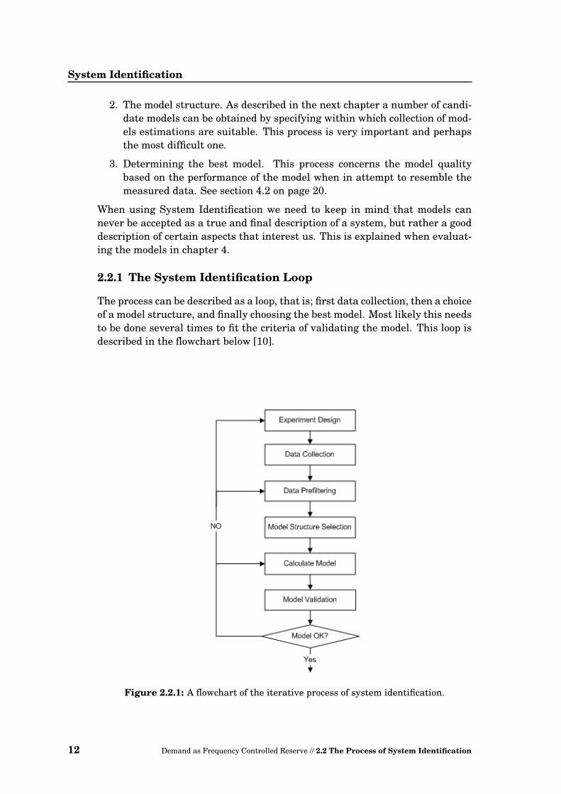
2.2.1 The System Identification Loop
The process can be described as a loop, that is; first data collection, then a choiceof a model structure, and finally choosing the best model. Most likely this needsto be done several times to fit the criteria of validating the model. This loop isdescribed in the flowchart below [10].
Figure 2.2.1: A flowchart of the iterative process of system identification.
12 Demand as Frequency Controlled Reserve // 2.2 The Process of System Identification

Chapter 3Estimations in SIT
System identification can now be performed on the data, and this chapter coversthe estimation process in MATLAB. First step is finding a handful of promisingestimations to examine more thoroughly later on. To derive a transfer functionfrom the collected data SIT is a very strong tool. Is does not necessarily giveout a TF but makes estimation polynomials that is polynomials that fit the datawhen combined in a certain manner i.e. the structure of the model.
Before estimations can be performed in SIT it is necessary to know a bit abouthow to do it and which class of model will have a good chance of fitting. Other-wise the number of estimations performed will easily increase without bringingbetter results. For a detailed review of the actions in SIT see appendix B frompage 59: “How To in SIT”.
3.1 Options and Preparing
Before starting estimation calculations in SIT a model should be roughly con-sidered and a class chosen. It is necessary to prepare the data for estimations,depending on class which again is chosen with consideration among SIT’s op-tions. The type of modeling is recognized as black box i.e. only the input andoutput data can tell anything about the system. Further a class of models ischosen from those available in SIT. Correlation modeling is not the issue withthis modeling even though we will consider it later c.f. section 4.2.1 on page 20.Spectral models are discarded because our data is in time domain. Left is pro-cess models and parametric models the latter having many different structures.
When performing a process model we noticed the limitations in number of zeros(only one) and a few number of poles, plus the estimation is continuous timebased. This did not seem to be quite adequate to make a fitting model, so thefocus lies on the parametric models. This class also have the options ‘State-Space’ and ‘By Initial Mode’. Neither gave good estimations in this case, andthe four remaining are all described by the general equation:
A(q)y(t) =[Bi(q)Fi(q)
]ui(t− nki) +
[C(q)D(q)
]e(t)
3.1.1 Basic Equations and Options
Options for the chosen model class is structure e.g. ARX or OE, orders of zeros,poles, delay etc. and a few others depending on the structure. The order of zeros,
13
Estimations in SIT
poles and delay are those we wish to vary, the rest should be fixed options. Theequation above gives four special cases, their equations are:
ARX : [A]y = [B]u + e (3.1.1a)ARMAX : [A]y = [B]u + [C]e (3.1.1b)
OE : y = [B/F ]u + e (3.1.1c)BJ : y = [B/F ]u + [C/D]e (3.1.1d)
Where the model gives options to choose focus, this should be given as ‘Simula-tion’ for the best result. Except for OE the possibility ‘Prediction’ is also avail-able but gives a poorer result. For the structure type ARX the options ARX andIV are available for calculating the residuals. The first one covers the method‘Least-Squares’, the second ‘Instrumental Variables’ and the first one is the onewe use. That is the standard relation known from Statistic Techniques whichis easily interpreted, while the second tries to shape the residuals according toinput and output, often making the model unstable.
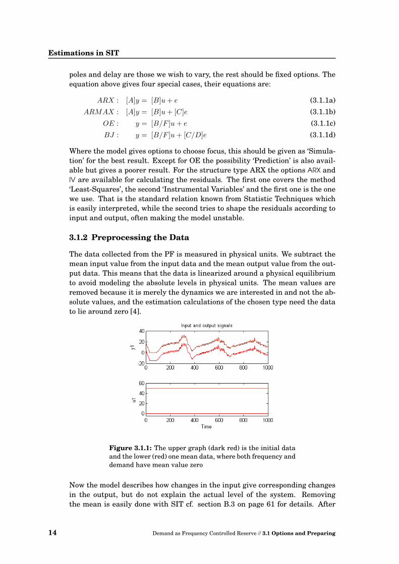
3.1.2 Preprocessing the Data
The data collected from the PF is measured in physical units. We subtract themean input value from the input data and the mean output value from the out-put data. This means that the data is linearized around a physical equilibriumto avoid modeling the absolute levels in physical units. The mean values areremoved because it is merely the dynamics we are interested in and not the ab-solute values, and the estimation calculations of the chosen type need the datato lie around zero [4].
Figure 3.1.1: The upper graph (dark red) is the initial dataand the lower (red) one mean data, where both frequency anddemand have mean value zero
Now the model describes how changes in the input give corresponding changesin the output, but do not explain the actual level of the system. Removingthe mean is easily done with SIT cf. section B.3 on page 61 for details. After
14 Demand as Frequency Controlled Reserve // 3.1 Options and Preparing

3.2 Performing Estimations
the identification, it is easy to add a constant to the model for transformingthe output back up to the correct level as in subsection 6.2.1 on page 37. Thedataset is now meandata which means that both frequencies and demands liearound zero see figure 3.1.1 on the preceding page, and it will be this mean datathat is the base of estimations.
3.2 Performing Estimations
When estimating MATLAB performs a lot of demanding numerical calculations,which means that the results can vary slightly even with the same data as ba-sis. Also the settings when performing is important and all estimations shouldbe saved for later recalling, since a repetition does not necessarily give the ex-act same model polynomials and the sensitivity is high. Further more they areestimated in discrete time.
When setting the parameters poles, zero and delay, the delay should be rathersmall, since this is how the PF system has been built. Also models with noise isunwanted, since no noise is supposed to occur in the simulation in PF, but for abroad investigation we nevertheless include a few noise models .
3.2.1 The set of Main Estimations
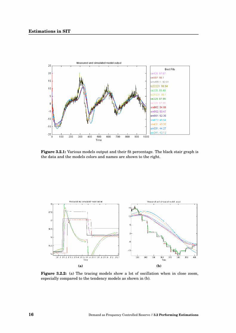
The main estimations are performed with meandata as base. However somemodels of the type ARX became unstable, so estimations have also been donewith another dataset as base, data1088d, as described in subsection 3.2.2 onpage 17. When estimating the first thing to do is viewing the graph of themodel compared to the data, and the best fit percentage. We tried a smallnumber of each model structure available and adequate in SIT, and exploredtheir behavior. The first two is ARX and ARMAX, where the only difference isthe noise parameter nC connected to the error e see (3.1.1a). The second pairis OE (Output-Error) and BJ (Box-Jenkins) and again BJ models include noisewith parameters nC and nD see (3.1.1d) while OE does not.
As depicted in figure 3.2.1 on the next page the ARX, ARMAX, OE and BJ canbe divided in two groups: Those with the highest fit percentage stick to the stairshape of the data like a tracing device, and those with a much lower percentageshow only the tendency see also figure 3.2.2 on the next page. The type ARX isof the latter and the rest is tracing models. Despite the close relation betweenARX and ARMAX, the behavior drastically changes when including the noise.
When zooming in on the tracing type, it becomes clear that the spikes on thegraph come from the model’s response when data rise or fall causing overshootssee figure 3.2.2 on the following page. The tendency models have a poor fit butit is easy to see just by looking, that it catches the basic behavior in a moresmooth way. When zooming in extra it is exposed that the smoothness is nottotal, the models have spikes, but a lot smaller than those for the tracing type.
15
Estimations in SIT
Figure 3.2.1: Various models output and their fit percentage. The black stair graph isthe data and the models colors and names are shown to the right.
(a) (b)
Figure 3.2.2: (a) The tracing models show a lot of oscillation when in close zoom,especially compared to the tendency models as shown in (b).
16 Demand as Frequency Controlled Reserve // 3.2 Performing Estimations

3.2 Performing Estimations
3.2.2 Estimations on Different Dataset
Some of the models based on the the dataset reaching from 1,000 to 2,000 sec-onds became unstable when transported out of SIT and into a transfer function.The reason is most possible the round off to four digits, since for this type ARXthe poles lie so close to the limit of the unit circle, that 5 or 6 digits have to beused to tell the difference. This is also a part of the reason why it is necessaryto compare the models from SIT with the TF as in chapter 5.
The dataset data1088d is the dataset used from the time 1,088 with mean atzero. This new dataset is used because of the ARX’s behavior in the beginningwhen trying to follow the tail that drops to zero as shown in figure 3.2.3 below.From this dataset the ARX models are redone, all the same as before plus two
(a) (b)
Figure 3.2.3: (a) The first 88 seconds of data (black) and ARX (colored). (b) A closerlook on the overshoot from the ARX models in the first second.
extra ARX10108 and ARX311 to reach both extremes with the estimations. Asfigure 3.2.4 on the following page shows when compared to page 16, figure 3.2.1,the models now look very different even though made in the same manner. Twoof the old models become unstable when re-estimated on the new data; ARX431(orange) and ARX551 (dark blue). This shows the importance of the choiceof dataset. Now we explore if the initial problems from before are still there,the smoothness of the models and their tendency/tracing display. As shown infigure 3.2.4 and figure 3.2.5 (a) on the next page most models still show onlythe tendency, the ARMAX (grey) being the exception and with ARX552 (violet)as sort of neither one. The models still oscillate the first second, but much lessas figure 3.2.5 (b) on the following page shows compared to figure 3.2.3 (b) onthe current page. The first models have swing above 20 MW while these rangewithin 2 MW for the first second.
The models to examine closer are the five OE and two BJ based upon meandata,and based upon data1088d the ARMAX and nine ARX. From the ARX mod-els three have already been deemed unusable but a methodical walk-throughshould reveal more clearly why it is so.
17

Estimations in SIT
Figure 3.2.4: ARX model outputs and their fit percentages. Some of the models areunusable.
(a) (b)
Figure 3.2.5: (a) The data and the stable models, zoomed in to trace view behavior. (b)The first second when estimated from the new dataset.
18 Demand as Frequency Controlled Reserve // 3.2 Performing Estimations
Chapter 4Evaluating the Models
After performing a rather large number of estimations, and only discardingthe most obvious failures it is necessary to use some tools for evaluating therest, these being the theory of regulation, correlations and the plot tools in SIT.When the evaluation is done, only two models should be presented to MATLAB
for further investigation.
The requirements for the model are a good fit, random residuals, low FPE andloss (autocorrelation can be high for OE and still be acceptable), and of coursethe model must be stable under all circumstances. Further more it should notbe to slow (settling time less that 400 s), not oscillate but have a high enoughorder to describe the complex behavior and still not cause great overshoot! Topass this judgment the theory is first represented and then the conclusion.
4.1 Theory of Regulation Technique
4.1.1 Zeros and Poles
When working in discrete time the zeros and poles show their significants bytheir placement in a Zero-Pole plot. The poles are normally marked with X’esand the poles with O’s. Drawing the unit circle, all poles should lie within thisfor stability. When placed upon the circle, the system becomes marginally stableat best. A complex pair of poles usually means the system is underdamped,leading to oscillation and a slower step response.
Also the placement of zeros according to poles has significants. A zero placedclosely to the pole will minimize the impact of it, although not determine itcompletely. The placement of poles and number of zeros can vary from discreteto continuous time depending on the transformation method.
4.1.2 Step and Impulse Responses
These two responses give a great amount of information about the system, andare normally regarded in continuous time. The step response shows the stan-dard behavior when reacting to at step up from the input. If it has overshootthe system is underdamped, and may even oscillate for a long time. If it risesvery slowly then it is overdamped and may react to slowly to response correctlyto the next impact. Optimum is critically damped, which is to say no com-plex poles, but often the best systems are slightly underdamped. The impulseresponse tells whether or not a system is able to react to sudden and violent
19

Evaluating the Models
impacts. It should return to zero rather fast and preferably without oscillation.
From the two responses some characteristics are revealed e.g. rise time, settlingtime, peak a.s.o. Since the stability and the reaction speed is important, we willconcentrate on the settling time, that is the time from the action till the timewhen settling is 98% done.
4.2 Using the SIT Tools
The important graphical representations are all available in SIT either as ModelViews or by using the LTI viewer cf. appendix B page 67. This means that mod-els can be eliminated due to unwanted behavior and by evaluating the modelsfit i.e. both the fit and the residuals.
4.2.1 Significance of Correlation
Correlation is a concept from Statistics and implies the co-variation betweenthe data and the model (autocorrelation). If the correlation is -1 or 1, then thetwo parameters follow each other perfectly either reciprocal or positive. Whencorrelation is zero, the two parameters are unbound, thus when showing resid-uals correlations they should lie close to zero, to indicate the relations in themodel are correct and sufficient.
4.2.2 Model Failure
For the models that show only the tendency (ARX) a failure exposes itself al-ready in the model output as on page 18, figure 3.2.4 with a negative fit per-centage. This behavior is not observed with the tracing models, since they stickto the stair graph even when oscillating. Even if these models obviously fail,their FPE, loss and residuals match the other ARX, so these parameters alonecan not designate the model. They seem unstable and this we will use for thefurther investigation.
4.2.3 Model Evaluation
All figures are placed in appendix C from page 71 to make the text coherent.The sections below are summaries of what is easily seen when going throughthe figures.
Judging the Models Condition by Noise, Resid-uals, Loss and FPE
First review is the model noise, and those with most noise are all ARX. Fromthe residuals only the ARMAX stands out from that type, whereas for the OEand BJ type, three models give them self away. For loss and FPE no tendencymodel lie above 0.02 and ARMAX has approx. 0.03 and that is very good. ForOE the loss and FPE lie in another band, though the highest order OE’s and BJ
20 Demand as Frequency Controlled Reserve // 4.2 Using the SIT Tools

4.3 Comparison to Other Datasets
lie beneath 1, the three other OE’s lie from 209 to 305. All the models that standout in these graphs will be investigated further for stability in next paragraph.
Judging the Models Stability by FrequencyResponse, Zero-Poles and Step/Impulse Responses
By looking at the frequency responses, even more models have unwanted be-havior, and some give surprises since they do not show signs of instability. Ex-amining the poles and zooming in shows that seven models fail to be stable.Combined with the models that have bad residuals (one being recurrent) andthe three models with noise (two being recurrent), 11 models fail and six re-main; two OE and four ARX.
The step and impulse responses are viewed in figure C.8 on page 74 for the twoOE with a higher order OE, and the four ARX with the ARMAX. This showsvery clearly why OE431 and ARMAX are not good since the oscillations areprofound. Also two more ARX are discarded due to oscillating impulse response,and two of each is left;
OE331 & OE221, ARX331 & ARX341.
Choosing one of each is easy, based on what we have already seen. The ARX341is slower than 400 s and OE331 fits the slightly underdamped presumption.And figure C.6 (b) on page 73 holds a powerful argument, since the two modelsshow no sign of falling frequency response unlike the others. Also OE331 andARX331 have the better fit percentages, although the difference is inconsider-able it is maintained when comparing to other datasets. Comparison to severaldataset is the next subject when we cross-compare the models to the datasets,and also consider the first seconds of the simulation.
4.3 Comparison to Other Datasets
Since we did not use the same dataset and both fit and residuals change ac-cording to the validation data, the OE model based on meandata is comparedto data1088d and vice versa. Also both models are compared to the startdata, tosee whether or not they can manage to swing in the correct way, even thoughnot based upon this data.
Cross Comparison
The ARX model returns to the former swing in behavior the first second low-ering the fit percentage, but still shows the tendency clearly. The OE fallsto a 85.6% fit, which is still fine but has worse residuals when compared todata1088d, though only slightly. The models do pass a validation to each othersdatasets.
21

Evaluating the Models
The Start
In the PF simulation it is clear that the system needs some time to swing into steady state, and data from this is startdata which is now imported to SIT,preprocessed and used for validation. The output and fit percentages are shownin figure 4.3.1 below. According to SIT both models will do well; The residuals
Figure 4.3.1: Both models follow the start data fine
are also fine and although the ARX swings again it follows the data very good.This is reassuring for the coming quest of using the TF in PF, since the start ofthe simulation is very important. If the TFs should prove useful at all they willhave to find a steady state similar to that of the heater block they are supposedto resemble.
4.4 Exporting the Models
Round off means having to analyze and compare the SIT model with constructedTF model. Focus is especially on the stability of the TF since the poles in SITlie very close to the limit. In the case of ARX331 it is necessary to use the polesfound in SIT to specify the parameters in the polynomials in order to make theTF and the SIT model identical see subsection 5.1.1 on page 24.
The polynomials from SIT without the parameters deviation are:
B(q) = −1551 q−1 + 2068 q−2 − 518.2 q−3 (4.4.1a)F (q) = 1− 1.712 q−1 + 0.5082 q−2 + 0.2054 q−3 (4.4.1b)
B(q) = −43.57 q−1 + 85.55 q−2 − 41.98 q−3 (4.4.2a)A(q) = 1− 2.055 q−1 + 1.112 q−2 − 0.057 q−3 (4.4.2b)
22 Demand as Frequency Controlled Reserve // 4.4 Exporting the Models

Chapter 5The Transfer Function
This chapter contains information about how the polynomials just derived canbe transposed into discrete transfer functions (TFs) which describe the heatersbehavior when controlled by the frequency. The TFs are then converted intocontinuous time and compared to their responses found in SIT to make surethey are correct. The continuous time TFs are then models describing the re-action of the heaters, and system properties e.g settling time, rise time anddamping are determined from analysis.
5.1 Deriving TF From SIT Polynomials
A TF H(s) is a mathematical representation between the ratio of the input andthe output of a system. For a linear time-invariant system (LTI) with a contin-uous input x(t) and output signal y(t), it’s Laplace transformation is describedby the equation:
H(s) =L{x(t)}L{y(t)}
=Y (s)U(s)
=bmsm + bm−1s
m−1 + ... + b1s + b0
sn + an−1sn−1 + ... + a1s + a0(5.1.1)
Correspondingly the discrete LTI transfer function is:
H(z) =Y (z)U(z)
=c0 + c1z
−1 + ... + cm−1z−m−1 + cmz−m
z−1 + d1z−2 + ... + dn−1z−n−1 + dnz−n(5.1.2)
The TF holds information about the system dynamics values where n is thesystem order, the denominators roots are the systems poles and the nominatorsroots are the systems zeros. The continuous LTI system is stable if and only ifall the poles are in the left coordinate plan and the discrete system is stable ifand only if all the poles are inside the unit circle. See section 4.1 on page 19 fora more general theory.
23
The Transfer Function
5.1.1 From Polynomials to TF
The models from SIT are discrete polynomials found from the dataset from PFMain Case. They are used to derive a discrete TF by using the relation of thepolynomials. SIT gives this discrete-time structure equation for OE:
y(t) =B(z)F (z)
u(t) + e(t) (5.1.3)
And for ARX:
A(z)y(t) = B(z)u(t) + e(t) (5.1.4)
As mentioned previously the poles of the polynomial models in SIT can becomeunstable when extracted into MATLAB because of the roundoff. This happenswith ARX TF and that is why we use the poles/zeros displayed in SIT to fix theARX TF as seen when comparing the polynomials equation (4.4.2) on page 22and the TF equation (5.1.6) on this page. By doing this the parameters in theTF become more detailed (more digits) and as the next section will show it’sstability is reestablished.
By using the above and equation (5.1.2) we can represent the polynomials asdiscrete (edited) transfer functions:
Hoe(z) =B(z)F (z)
=−1551 z−1 + 2068 z−2 − 518.2 z−3
1− 1.712 z−1 + 0.5082 z−2 + 0.2054 z−3(5.1.5)
And
Harx(z) =B(z)A(z)
=−43.57 z−1 + 85.571044 z−2 − 42.00106 z−3
1− 2.05492 z−1 + 1.1119147 z−2 − 0.05699436 z−3(5.1.6)
Assuming e(t) = 0. By a simple command in MATLAB filt(B,F,Ts), the function filtgives a discrete transfer functions where B and F are the polynomials constantsin an ascending power of z−1, and Ts is the sampling time of the dataset fromPF.
5.1.2 From Discrete to Continuous Time
The TF is now operational in discrete time, but normally transfer functions areused in continuous time, so the TF should be transformed for further use. Toadapt the transfer function to continuous time we use a method called ‘tustin’which is based on an exponential function in the z-transform, where:
z = eTs ∼=1 + T
2 s
1− T2 s
(5.1.7)
This calculation can be tedious, but MATLAB has a simple command calledd2c(dH,‘tustin’), which calculates the continuous transfer function very fast. Itis also possible to use a method called ’zero order hold’ but that method pro-
24 Demand as Frequency Controlled Reserve // 5.1 Deriving TF From SIT Polynomials
5.1 Deriving TF From SIT Polynomials
duces a continuous system with a higher order because negative real poles inthe domain are mapped as pairs of complex poles.
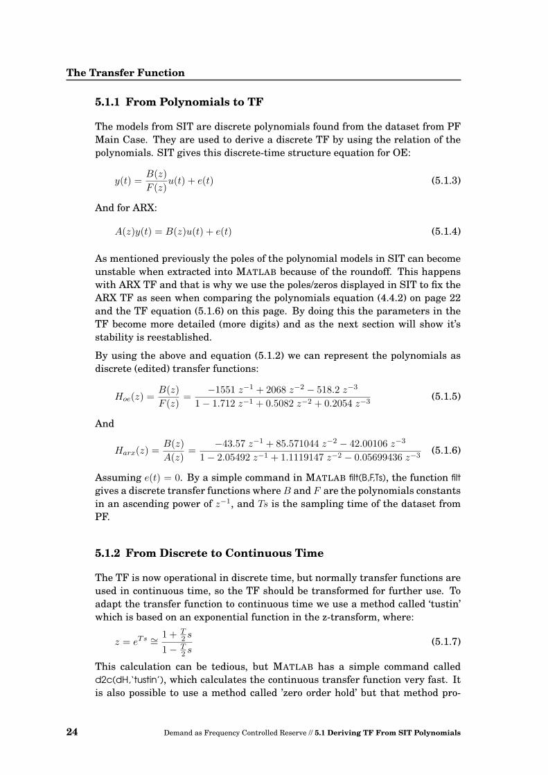
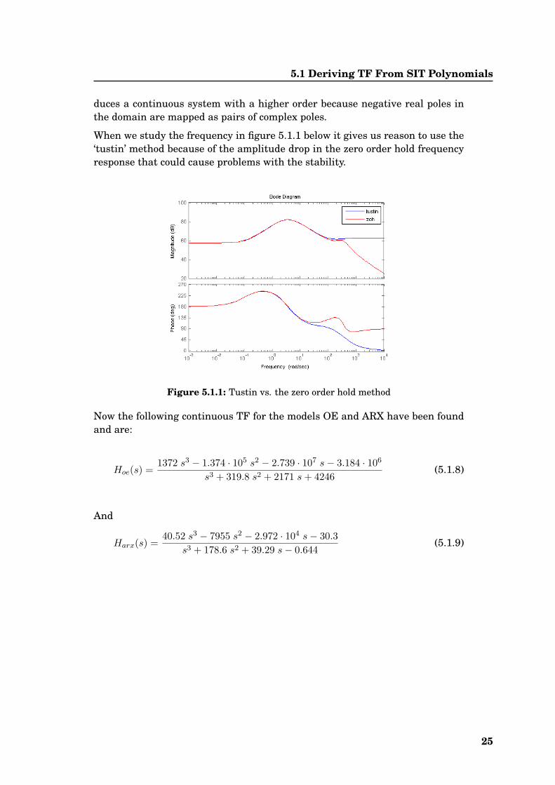
When we study the frequency in figure 5.1.1 below it gives us reason to use the‘tustin’ method because of the amplitude drop in the zero order hold frequencyresponse that could cause problems with the stability.
Figure 5.1.1: Tustin vs. the zero order hold method
Now the following continuous TF for the models OE and ARX have been foundand are:
Hoe(s) =1372 s3 − 1.374 · 105 s2 − 2.739 · 107 s− 3.184 · 106
s3 + 319.8 s2 + 2171 s + 4246(5.1.8)
And
Harx(s) =40.52 s3 − 7955 s2 − 2.972 · 104 s− 30.3
s3 + 178.6 s2 + 39.29 s− 0.644(5.1.9)
25

The Transfer Function
5.2 Analyzing the TF
In the process of analyzing the TFs, it is very important that the responses ofthe discrete TFs are compared to the ones found in SIT cf. the roundoff problemdiscussed previously when the polynomials are exported from SIT to MATLAB.This kind of problem occurs especially when the poles and zeros lie close to theunit circle. This is important because the TF is very sensitive and can becomeunstable if the parameters vary even on the fifth or sixth digit. Also we willmake sure that we have not made errors in the beginning when the polynomialswhere copied from SIT and into vectors representing the constants to build aTF.
The Step and Impulse responses are compared for the OE in figure 5.2.1 on thefacing page and for ARX in page 28, figure 5.2.3. Furthermore the responses ofthe discrete TFs and continuous TFs are compared to make sure that they be-have the same way. When comparing responses we use Step response, Impulseresponse and Bode plots.
A comparison of settling times (marked with a dot in the graphs) in the re-sponses, figures 5.2.1 and 5.2.2, show that the the settling time in the discreteOE TF is 1.64 s which is a little bit slower than for OE from SIT which is 1.3 s.This is most likely because of some small roundoff difference. The settling timefor the impulse response is pretty much the same, or around 1.2 s for both,which is very good since it indicates that the discrete TF is correctly presentedfrom SIT to MATLAB.
When plotting the responses of the ARX model in the beginning there weresome problems regarding the stability of the model because of the poles asmentioned previously. The poles have been fixed by trial and error from theSIT pole/zero plots and should now behave correctly and be stable.
The settling time for the step response for ARX in SIT figure 5.2.3 on page 28 isaround 300 s and 240 s for the discrete ARX figure 5.2.4 on page 28. The impulseresponse is very similar and that results in the decision that the edited ARX TFis valid.
5.2.1 Step and Impulse Responses
The discrete responses for OE are showed in figures 5.2.1 and 5.2.2, and thediscrete responses for ARX is shown in 5.2.3 and 5.2.4, both pairs displayingfirst the SIT and then the MATLAB response.
In figure 5.2.2 on the next page and figure 5.2.5 on page 29 we see that the stepresponse for the discrete TF Hoe(z) and continuous TF Hoe(s) are the same, butthe impulse response is not; the difference is a factor of 3, 000 in the down shoot.This happens when the TF is converted from discrete time to continuous time.As seen in equation (5.1.8) on the previous page the nominator is very largecompared to the nominator in the discrete equation (5.1.5) on page 24.
26 Demand as Frequency Controlled Reserve // 5.2 Analyzing the TF

5.2 Analyzing the TF
Figure 5.2.1: Step/Impulse responses for the discrete polynomials, OE.
Figure 5.2.2: Step/Impulse response for discrete TF Hoe(z).
27

The Transfer Function
Figure 5.2.3: Step/Impulse responses for the discrete polynomials, ARX.
Figure 5.2.4: Step/Impulse responses for the discrete TF Harx(z).
28 Demand as Frequency Controlled Reserve // 5.2 Analyzing the TF

5.2 Analyzing the TF
The same thing happens for the ARX TF see figures 5.2.4 on the preceding pageand 5.2.6 on this page; the down shoot is also a factor of 3,000 bigger in thecontinuous case. This property is used in the next chapter when the TFs areincorporated in PF.
Figure 5.2.5: Step/Impulse response for the continuous TF Hoe(s).
Figure 5.2.6: Step/Impulse response for the continuous TF Harx(s).
29

The Transfer Function
5.2.2 Bode Plots
Bode plots are used to compare the magnitude and phase of the TFs. A mag-nitude bode plot is a graph of magnitude in dB versus the frequency in a log-arithmic axis, and a Bode phase plot is a graph of phase versus the frequency,also plotted in logarithmic axis. If the Bode plot shows that the amplitude keepfalling as the frequency rises, the system should be examined for unstability.According to the Bode plot figure 5.2.8 there are a slight difference in the dis-crete and continuous systems, but these small differences are negligible and donot effect the system in PF.
Figure 5.2.7: Bode plot for both OE(green) and ARX(blue) from SIT
Figure 5.2.8: Bode plot for both OE and ARX TF, fom MATLAB
30 Demand as Frequency Controlled Reserve // 5.2 Analyzing the TF

5.3 Visualizing the TF in MATLAB Simulink
5.3 Visualizing the TF in MATLAB Simulink
Next the accuracy of the TFs are investigated when the initial data from PF isused as an input. Small models, in MATLAB Simulink have been made for eachof the TFs, OE and ARX in Simulink. These models take the initial data as aniddata input and the polynomials from equations (4.4.1a) to (4.4.2b) as a idpolymodel giving the power as output i.e. y(t) = H(s)u(t).
Figure 5.3.1: Simulink model of the TF, where the input data is the frequency fromthe original PF system.
By plotting the power demand for both OE and ARX models it is clear that someproblems occur in the output of the TF model see figures 5.3.2 and 5.3.3. Eventhough the TFs do follow the data while going toward steady state they do nothave the correct level and do not behave as wanted right at the time of event;the demand rise in stead of falling. This applies for both models.
In figure 5.3.1, M is an idpoly model, made from the polynomials from SIT, seeequations (4.4.1a) through (4.4.2b) page 22.
Figure 5.3.2: The power demand and the frequency demand of the OE model whenSimulated in MATLAB Simulink with the frequency input from the original PF model.
When the entire data from PF is used to validate the two models the reasons forsome of the problems become known. From 5.3.4 we see the opposite response
31

The Transfer Function
Figure 5.3.3: The power demand and the frequency demand of the ARX model whenSimulated in MATLAB Simulink with the frequency input from the original PF model.
behavior in the power demand at 1,000 s and the wrong level allready in SIT.
Now we see that we need to make some modifications to our TF before imple-menting in PF, because of the opposite response of the power demand and thevalues of the power, see subsection 6.2.1 on page 37.
Figure 5.3.4: The two models and the entire PF data (0 s-2000 s) mean around zero.
32 Demand as Frequency Controlled Reserve // 5.3 Visualizing the TF in MATLAB Simulink
5.4 Concluding Remarks
5.4 Concluding Remarks
In this chapter the use of TFs describing a system has been clarified. We haveseen that the two models are stable, have reasonable shapes and short risetimes. The settling is slow for ARX and fast for OE and their steady values aredifferent but the plots for the models are comparable in shape.
In future references it should be studied more carefully the method of convert-ing between discrete and continuous time, specially the difference of the im-pulse response. Also, the roundoff from SIT to MATLAB can cause unexpectedproblems, and our experience shows that the parameters in the TF are indeedvery sensible, changing the look of the responses significantly when editingeven the fourth or fifth digit after the decimal.
When using the total dataset from the main simulation in PF, the output fromboth models show an unexpected and unwanted reaction to the event. Compar-ing figure 5.3.2 on page 31 to figure 1.3.1 on page 9 it seems that the outputfrom the TFs when reacting to the event resembles the grid power instead ofthe demand. When incorporating the TFs in PF as done in chapter 6 we makeadjustments to the TFs in order to eliminate this problem.
33


Chapter 6TF in Main Case PF
This chapter contains information about using the derived TFs in PF, compar-ing the power demand produced by each TF and choosing the best one. Theaim is to validate the use of the derived TFs in relation to the system in whichthe simulations are originally performed. If the model can perform in a similarmatter as the original heater block, the TF model is acceptable and the modelvalidated for this use.
6.1 Preparing new Simulations in PF
6.1.1 Converting to State-Space Form
The continuous transfer function needs to be converted into a State-Space model(SS) before it can be implemented into PF. The SS representation can describethe system by the equations:
x = Ax + Bu (6.1.1)y = Cx + D u (6.1.2)
Where x is a vector describing the states, u is the input and y is the output. Thematrices A, B, and C determine the relationships between the states, input andoutput variables. If the transfer function is represented in the form of equation(5.1.1), we can find the variables by using the matrix-form:
x1
x2...
xn−1
xn
=
0 1 0 . . . 0 00 0 1 . . . 0 0...
...... . . .
......
0 0 0 . . . 1 0−a0 −a1 −a2 . . . −an−2 −an−1
x1
x2...
xn−1
xn
+
00...01
u
The output equation is:
y =[
b0 b1 . . . bn−2 bn−1
]x + bnu (6.1.3)
The matrix elements of the SS model have the same number of coefficients asthe TF model, apart from the zeros and ones, these are the only parameters inthe model. The coefficients of the denominator are the last row of A with oppo-site signs and in reverse order. And the coefficients of the numerator are foundin C in reverse order. The D matrix is zero when the numerator polynomial isof a lower order than the denominator.[2]
35

TF in Main Case PF
When working in MATLAB it is very easy to convert the continuous TF into SS,this is done with the command ss(H) where H is a continuous TF, which givesthe A, B, C, and D matrices.
6.1.2 Creating a PF Macro From the TF
A new model is built in PF corresponding to the TF found in SIT. Here the dif-ferential states are defined and the coefficients in DIgSILENT as in figure 6.1.1below. By doing this we have an equation representing all the states of theTF which describes the system and now it is possible to investigate the powerdemand when controlled by the frequency.
Figure 6.1.1: The states of the TF, made in a macro in PF
6.2 First Simulations Experiences
The case in PF is adapted with the new macro, and simulations should be donein a way that allows comparison to the main simulation. Now connected tothe grid is our TF model in SS form and the same load event as discussed inchapter 1 with a load event of 100 MW at 1, 000 s. The power demand of the OEand ARX SS models are investigated according to the frequency, at the eventmaking sure there is a frequency reaction to investigate. To make the macromodel behave in the wanted way, some adaptations have to be done however.
36 Demand as Frequency Controlled Reserve // 6.2 First Simulations Experiences
6.2 First Simulations Experiences
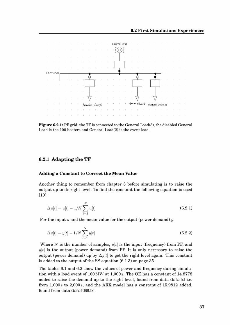
Figure 6.2.1: PF grid; the TF is connected to the General Load(3), the disabled GeneralLoad is the 100 heaters and General Load(2) is the event load.
6.2.1 Adapting the TF
Adding a Constant to Correct the Mean Value
Another thing to remember from chapter 3 before simulating is to raise theoutput up to its right level. To find the constant the following equation is used[10]:
∆u[t] = u[t]− 1/NN∑
t=1
u[t] (6.2.1)
For the input u and the mean value for the output (power demand) y:
∆y[t] = y[t]− 1/N
N∑t=1
y[t] (6.2.2)
Where N is the number of samples, u[t] is the input (frequency) from PF, andy[t] is the output (power demand) from PF. It is only necessary to raise theoutput (power demand) up by ∆y[t] to get the right level again. This constantis added to the output of the SS equation (6.1.3) on page 35.
The tables 6.1 and 6.2 show the values of power and frequency during simula-tion with a load event of 100 MW at 1,000 s. The OE has a constant of 14.8778added to raise the demand up to the right level, found from data data.txt i.e.from 1,000 s to 2,000 s, and the ARX model has a constant of 15.9812 added,found from data data1088.txt.
37

TF in Main Case PF
Multiplying With a Constant due to ImpulseResponse
As mentioned in chapter 5 the down shoot in the impulse response gives a big-ger value in continuous time, to solve this we need to multiply the continuousTF and the SS output equation 6.1.3 with a constant of (0.003) to get the samelevel as for discrete time for which the TF is initially built.
The impulse response is the response of the TF to a direct δ input. The Laplacetransformation of the unit impulse is L{δ(t)} = 1, and the Z transform isZ{δ(kT )} = 1, where kT = t, so the impulse response for both discrete andcontinuous should be the same:
h(t) = 1 · TF (s) and h(kT ) = 1 · TF (z) (6.2.3)
The impulse responses are shown for both models in figure 6.2.2 on the facingpage when the continuous and the SS models are multiplied with the constant0.003 while the discrete is directly from SIT. Then we get the same impulseresponse for the SS model which will be simulated in PF as the one in SIT.
The impulse responses both discrete and continuous need to be alike for theTFs because when implemented in PF it is the continuous SS TF that suffers aload event. This can be assumed to be like an impulse and it is necessary thatthe TFs behave as in SIT to avoid great swing.
Changing the Sign due to Opposite Event Re-action
As mentioned before the SS equation represents the 100 heaters and when sim-ulated it’s output should behave as frequency controlled reserve, that is whenthe frequency drops due to a load event it’s response should also drop, becausethe heaters should turn off to help the frequency rise again.
When forcing an event on both OE and ARX SS models the power demand riseswhen the frequency drops, see section 5.3 on page 31. That is why a minus isnow multiplied to get the demand to react correctly to an event.
The output equation is now:
y = −0.003 · (b0x1 + b1x2 + b2x3 + b3u[t]) + ∆y[t] (6.2.4)
6.3 The Behavior in Main Case
The simulation results are shown in figure 6.3.1 on page 40 and figure 6.3.2 onpage 41. When studied it is obvious that the graphs mostly resemble the steadystate of the former simulation in PF cf. page 9, figure 1.3.1. The frequency doesdrop a little when initially settling, and then drops again when event occurs butthe oscillations seen in the simulation from PF are efficiently gone.
38 Demand as Frequency Controlled Reserve // 6.3 The Behavior in Main Case

6.3 The Behavior in Main Case
Figure 6.2.2: The impulse response for the discrete TF, OE and ARX, compared withthe continuous and SS TF multiplied with the factor 0.003.
39

TF in Main Case PF
Figure 6.3.1: Power and frequency when Hoe,SS is describing the heaters.
6.3.1 The Event Reaction
As seen in chapter 5 the step response time is much faster for OE than for ARX,this is also seen here in the PF model see figure 6.3.1 below. The power demandwhen using the OE SS model reacts faster to change in the frequency than ARXin figure 6.3.2 on the next page. This can be a reason for choosing to use OEinstead of the ARX.
Furthermore the OE model shoots down and then a little bit up, resembling theheaters behavior in the main simulation; first turning everything off and thensettling at a new level. The down shoot is however very fast not providing thesystem with the wanted delay in power consumption that is supposed to giveother reservers time to cut in. See also table 6.1 on page 43.
The ARX model in PF drops slower and a bit less, actually it rises to almost thesame steady state value as before event cf. table 6.2 on page 43 especially com-pared to the significant drop. This seem reasonable enough since ARX from thebeginning has shown tendency rather than details. The power drop is howeverjust as small as for the OE model; about a factor of 1,000 to small.
The reason for the small drop in power demand could be because the frequencyis initially normalized, and then multiplied with 50 before displayed while ourmodel is based on not-normalized frequency.
A comparison has been made in to another system in PF see chapter 7 whenthe input is normalized and not multiplied with 50. This gives a more properdrop in the frequency. However the simulation is made for another reason i.e.breaking one of the loops in PF.
40 Demand as Frequency Controlled Reserve // 6.3 The Behavior in Main Case
6.3 The Behavior in Main Case
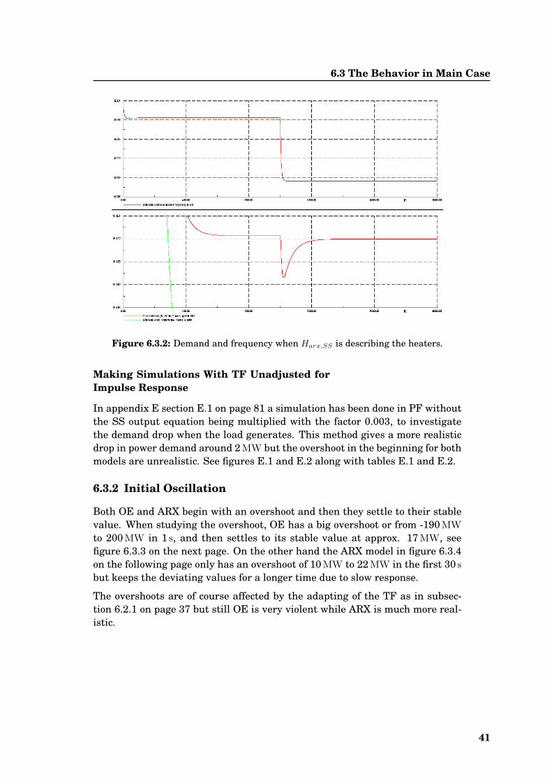
Figure 6.3.2: Demand and frequency when Harx,SS is describing the heaters.
Making Simulations With TF Unadjusted forImpulse Response
In appendix E section E.1 on page 81 a simulation has been done in PF withoutthe SS output equation being multiplied with the factor 0.003, to investigatethe demand drop when the load generates. This method gives a more realisticdrop in power demand around 2 MW but the overshoot in the beginning for bothmodels are unrealistic. See figures E.1 and E.2 along with tables E.1 and E.2.
6.3.2 Initial Oscillation
Both OE and ARX begin with an overshoot and then they settle to their stablevalue. When studying the overshoot, OE has a big overshoot or from -190 MWto 200 MW in 1 s, and then settles to its stable value at approx. 17 MW, seefigure 6.3.3 on the next page. On the other hand the ARX model in figure 6.3.4on the following page only has an overshoot of 10 MW to 22 MW in the first 30 sbut keeps the deviating values for a longer time due to slow response.
The overshoots are of course affected by the adapting of the TF as in subsec-tion 6.2.1 on page 37 but still OE is very violent while ARX is much more real-istic.
41

TF in Main Case PF
Figure 6.3.3: The overshoot in the OE SS model is from −190 MW to 200 MW.
Figure 6.3.4: The overshoot in the ARX SS model is from 10 MW to 22 MW.
42 Demand as Frequency Controlled Reserve // 6.3 The Behavior in Main Case
6.4 Concluding Remarks
6.3.3 Comparison
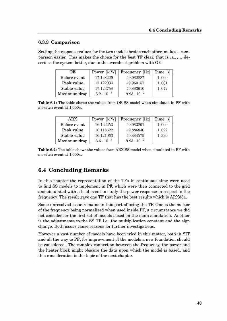
Setting the response values for the two models beside each other, makes a com-parison easier. This makes the choice for the best TF clear, that is Harx,ss de-scribes the system better, due to the overshoot problem with OE.
OE Power [MW] Frequency [Hz] Time [s]Before event 17.128229 49.982887 1, 000Peak value 17.122034 49.960157 1, 001
Stable value 17.123758 49.883610 1, 042Maximum drop 6.2 · 10−3 9.93 · 10−2
Table 6.1: The table shows the values from OE SS model when simulated in PF witha switch event at 1,000 s.
ARX Power [MW] Frequency [Hz] Time [s]Before event 16.122253 49.983891 1, 000Peak value 16.118622 49.886840 1, 022
Stable value 16.121963 49.884579 1, 330Maximum drop 3.6 · 10−3 9.93 · 10−2
Table 6.2: The table shows the values from ARX SS model when simulated in PF witha switch event at 1,000 s.
6.4 Concluding Remarks
In this chapter the representation of the TFs in continuous time were usedto find SS models to implement in PF, which were then connected to the gridand simulated with a load event to study the power response in respect to thefrequency. The result gave one TF that has the best results which is ARX331.
Some unresolved issue remains in this part of using the TF. One is the matterof the frequency being normalized when used inside PF, a circumstance we didnot consider for the first set of models based on the main simulation. Anotheris the adjustments to the SS TF i.e. the multiplication constant and the signchange. Both issues cause reasons for further investigations.
However a vast number of models have been tried in this matter, both in SITand all the way to PF; for improvement of the models a new foundation shouldbe considered. The complex connection between the frequency, the power andthe heater block might obscure the data upon which the model is based, andthis consideration is the topic of the next chapter.
43


Chapter 7Step Case
In the previous examples and calculations the TFs were built from a systemwhich has the frequency depending on the grid power. This chapter covers anexample when this loop is broken and a step function is used as frequency in-put instead of the frequency from the grid, making the TF independent fromthe electrical feedback of the system. This case study is called Step Case cf. [5].
7.1 Data From PF
Another system is built in PF, where the input is a step going from 1 down to0.998 at 1,000 s. The same block with the 100 heaters is simulated in order tomake a new dataset, only the relation constant kf is changed from 15 to 5 toavoid forcing the demand to zero for longer intervals since SIT has problemshandling the output when it goes to zero.
The dependency of the signals is changed as seen in figure 7.1.1 below whichshould be compared to the blockdiagram page 7, figure 1.2.1. This makes thedemand and the grid frequency change drastically as depicted in figure 7.1.2 onthe next page vs. figure 1.3.1 on page 9 that show the simulation from MainCase. The simulation is saved and the new dataset called PFstepdata is readyfor use in SIT.
Figure 7.1.1: The block diagram of the system with the feedback from the grid to theheaters broken, and a step as input frequency.
7.2 Estimating a Model in SIT
The same procedure is done here as described in chapter 3 and chapter 4, onlythe whole dataset is used when finding a model which describes the system i.e.
45

Step Case
Figure 7.1.2: Power and frequency of the 100 heaters with a step as input and a brokenfeedback loop between the frequency from the grid and the power output.
from 0 to 2000 s, because the input signal otherwise is zero after 1,000 s whenthe mean values have been extracted.
Figure 7.2.1: The stepdata; f and p with mean around zero. This dataset is used tofind a model in SIT.
46 Demand as Frequency Controlled Reserve // 7.2 Estimating a Model in SIT

7.3 Deriving the TF in MATLAB
It is not easy to find a model which describes the behavior of a system withsuch different input and output signals because SIT uses the change in inputto calculate the change in the output, and the input only changes once. Systemidentification may not be the best way to find a model for this kind of system,and the best fit is very low.
The best describing stable model is ARX521 and it follows all of the oscillationsquite well, see figure 7.2.2 below. The poles are stable, but the responses areslow with big oscillations, this causes problems further on when the model issimulated in PF.
Figure 7.2.2: The model chosen is ARX521, it’s best fit percentage is poor but it followsthe oscillation rather well.
The polynomials from SIT (unedited) are:
B(q) = 2.399q−1 − 2.399q−2 (7.2.1)A(q) = 1− 1.998q−1 + 0.9975q−2 − 0.01404q−3 + 0.02597q−4 − 0.01185q−5
7.3 Deriving the TF in MATLAB
Again the same method is used as in chapter 5 to built the TF from the polyno-mials (7.2.1). When doing this we experienced problems evolving the sensibilityof the model. That is SIT is limited to a number of digits and when computingthe TF in MATLAB two poles became unstable.
To prevent this we use the poles and zero plot from SIT and fix the poles totheir exact values. After this is done the responses are similar for the modelARX521 in SIT and the TF in discrete time built in MATLAB see figures 7.2.3and 7.3.1 on the following page. The continuous TF’s responses are equivalentto the discrete TF.
47
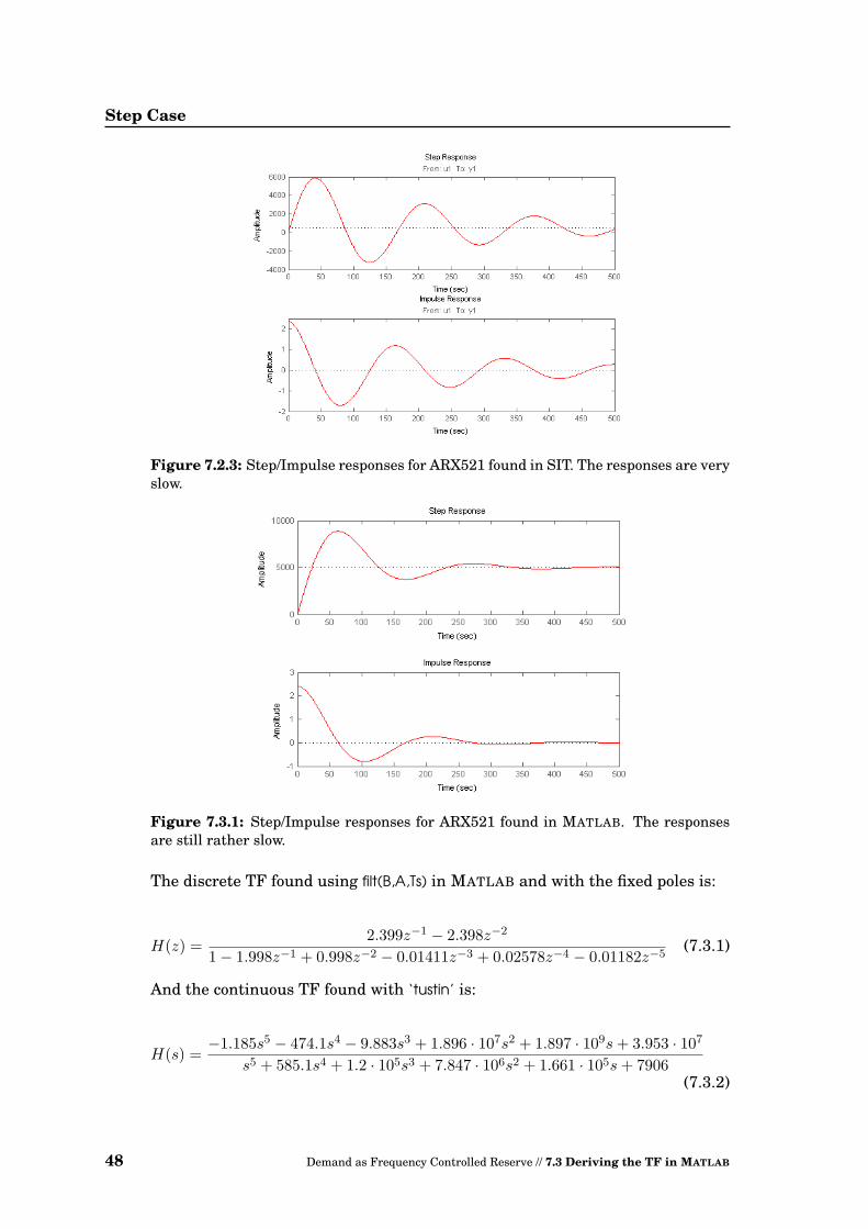
Step Case
Figure 7.2.3: Step/Impulse responses for ARX521 found in SIT. The responses are veryslow.
Figure 7.3.1: Step/Impulse responses for ARX521 found in MATLAB. The responsesare still rather slow.
The discrete TF found using filt(B,A,Ts) in MATLAB and with the fixed poles is:
H(z) =2.399z−1 − 2.398z−2
1− 1.998z−1 + 0.998z−2 − 0.01411z−3 + 0.02578z−4 − 0.01182z−5(7.3.1)
And the continuous TF found with ‘tustin’ is:
H(s) =−1.185s5 − 474.1s4 − 9.883s3 + 1.896 · 107s2 + 1.897 · 109s + 3.953 · 107
s5 + 585.1s4 + 1.2 · 105s3 + 7.847 · 106s2 + 1.661 · 105s + 7906(7.3.2)
48 Demand as Frequency Controlled Reserve // 7.3 Deriving the TF in MATLAB

7.4 Simulating in PF
7.4 Simulating in PF
The TF is then converted into SS form so it can be implemented in PF as a func-tion of it’s states. The new system built in PF is called DFRGloadAggstep.dz.Before simulating the new TF is implemented into a macro as before and con-nected to the grid instead of the heater block.
The input frequency is the measurement file stepdata and a load event of100 MW is cut in at 1,000 s as in the Main Case. The macro SS output equa-tion (6.1.3) on page 35 is added the power level constant ∆y[t] = 18.9537 foundfrom stepdata in the usual manner as discussed in subsection 6.2.1 on page 37.
The simulation results are showed in figure 7.4.1 below, where the power de-mand acts as FCL reserve. The oscillations in the beginning are very violentand long lasting and the steady state levels of both signals are wrong; the de-mand is extremely high and the frequency significantly low. At event the de-mand drops approx. 30 MW when f falls 0.03 Hz. In appendix E section E.2 onpage 83 the macro is placed differently and the outputs from the simulation arestill not adequate. Probably SIT is not capable of making a model that describesthis situation.
Figure 7.4.1: The power demand of the system with input/output loop broken.
7.5 Concluding Remarks
In this chapter we have investigated some of the properties in the PF modelthat could interfere with the abilities of the TF e.g. the loop, the normalizationof the frequency and the oscillating behavior of the frequency. It shows thatthe back loop between the demand and the grid properties as total demand andfrequency indeed have a large influence on the behavior of the FCLs.
When the heater block is simulated in PF it seems that the stability nearly van-ish; the bunching up is there but the smoothing out is not. The oscillating of the
49

Step Case
power and grid frequency are violent and persistent while the input frequencyis forced stable.
The order of the TF is higher for this modeling although probably it could gethigher. This clearly shows in the oscillating responses and if the precedingrequirements stated in chapter 4 were valid the ARX521 should have been dis-carded.
When the TF macro is simulated in PF as originally i.e. between net frequencyand demand it behaves unwanted and unexpected. When it replaces the heatersit reacts correctly but the oscillations are to violent. The forced frequency inStep Case is artificial, but this case with a step input reviled some characteris-tics of the FCLs that the former case did not. Models based on this case are notgood and ARX331 used in Main Case is still considered the most proper model.
50 Demand as Frequency Controlled Reserve // 7.5 Concluding Remarks

Chapter 8Conclusion
Reviewed About the TFs
In this project a number of transfer functions have been derived and placed inuse. The process and tools match the planned method as roughly reviewed inthe figure page 3 i.e. with MATLAB SIT as a very important component.
The TFs can in a theoretical matter describe the behavior very well, when look-ing only on the power demand depending om the frequency. In context with arepresentation of the Danish grid, the TF models can give an output either veryclose to what a simulation in PF would give (OE331) or just the tendency of thesame (ARX331), as long as no event occurs making the frequency skip. For atheoretical analysis the ARX331 model can give some information about thesystem which is not directly readable from simulations in PF such as settlingtime and stability. When a disturbance or an event occur however, the demandactually reacts opposite than expected in the second of the disturbance. Follow-ing, the reaction is as required.
When Used in PF
The transfer functions found in this project do describe the behavior of the ag-gregated loads constructed in PF. The degree of accuracy is debatable whenincorporated in PF since some adaptations have been done and the degree ofdetails lowered, but the basic behavior is caught by the models interacting withPF.
The PF Main Case is a complex system that binds the various signals tightlytogether in order to resemble the grid as much as possible. This gives a doubledependency between the frequency and the power and this is incorporated inthe first TFs. If measured frequency were input to these TFs the output wouldbe as if the FCLs were connected to the net and had influence on the frequency.
This caused the creation of an unbound frequency as a step function in a casewhere the frequency is a small normalized step down. This changed both thegrid frequency and the power demand drastically causing lots of oscillationsince the damping came from the effect of the grid to the frequency and thusto the demand. The new TF based upon this data with demand as output andstep frequency as input describes the FCLs only and does not include the effectfrom the net. Based upon that criteria the new TF should show more suitablebehavior in PF than the former TFs. The start oscillation does resemble theshape of the Step Case PF simulation more, but reaches unwanted levels. Infact Step Case is not suitable to make this kind of models.
51
Conclusion
Considerations taking in to account in the Step Case are those of the normalizedfrequency and another data basis with another kind of disturbance. Further-more, the TF model describes only the block containing the heaters and do notinclude grid elements.
Reviewed About the Method and Tools
For further investigations the data basis could be reconsidered. The main em-phasis in this project have been the total system with all original dependencyand after a controlled event. Perhaps more precise results could be reached byusing start data, another event or a system bound in a different matter e.g. asdone in Step Case. Further investigations could show if the small reactions ofthe demand are related to the normalization of the frequency in PF.
Aside from the basis of the model, the method and estimations could cause rea-son for further investigation. There are possibilities that the estimations arenot adequate and the method might provide these limitations. Since a numberof steps have been performed using specific tools, the outcome has all the limi-tations from each tool e.g. the round off in SIT and the way MATLAB performstransformation when translating the model first from SIT to continuous andthen to State-Space.
When adjusting the transfer functions to PF several actions have been done,some according to the theory of performing system identification i.e. the leve-ling constant, and others due to specific observations of the model i.e. multi-plying with a constant and changing the sign. We have done these adaptationsin order for the models to react properly when incorporated in PF. The latteradjustments are empirically based and raise an issue that could lead to a fur-ther investigation either of this process or in combinations with a review of theentire method.
Important Issues
By using the derived methods and examining the FCLs we have reviled someproperties of accumulated FCLs. It seems that the loads themselves are margi-nally stable, since a great part of the damping comes from the grid connection.The bunching up and smoothing out is only observed in simulations when theheaters are cut in to the grid.
The tools used might not be sufficient since SIT goes only as high as around the10th order and does not provide high accuracy. A change in tool is recommendedand an investigation taking the models to a much higher order.
The TFs found are stable and have the right steady state levels. They allrespond correctly to load events though the responses are very small. TheARX331 model gives the best results in PF but simulating with ARX in steadof the heater block show a loss in detail level. A further development of the TFcould solve the issue of the small response and make it a proper alternative tothe time demanding simulations in PF.
52 Demand as Frequency Controlled Reserve //

Bibliography
[1] Center for Elteknologi, Ørsted DTU & EA Energianalyse A/SElforbrug som frekvensstyret reserve, november 2005.
[2] Hendricks, Elbert; Jannerup, Ole and Sørensen, Paul HaaseLinear Systems Control, Deterministic and stochastic methods,September 2006, Ørsted DTU, Automation
[3] Jannerup, Ole and Sørensen, Paul HaaseReguleringsteknik, May 2004, 3. udgave
[4] Ljung, LennartSystem Identification, Theory for the User, 1999, Second Edition
[5] Xu, ZhaoAggregated Heaters Model in PowerFactory, 2006-2007,Source files: DFRloadAgg.dz and DFRloadAgg_step.dz
[6] Z. Xu, J. Østergaard, M. Togeby, C. Marcus-MøllerDemand as Frequency Controlled Reserve -Potentials and Perspectives,November 2006.
[7] Z. Xu, J. Østergaard, M. Togeby, C. Marcus-MøllerDesign and Modeling of Thermostatically Controlled Loads as FrequencyControlled Reserve, 2005.
53

BIBLIOGRAPHY
Other References
[8] Ljung, LennartGetting Started with System Identification Toolbox 7.0, March 2007,First printing New for Version 7.0 (Release 2007a).
http://www.mathworks.com/access/ helpdesk/help/pdf_doc/ident/ident_gs.pdf
[9] Ljung, LennartSystem Identification Toolbox User’s Guide, March 2007, Online onlyRevised for Version 7.0 (Release 2007a).
http://www.mathworks.com/access/helpdesk/help/pdf_doc/ident/ident.pdf
[10] Zhang, YouminF7-1: System Identification, Fall 2006.
http://www.cs.aue.auc.dk/ymzhang/courses/sysid/index.html
Downloaded March 2007
54 Demand as Frequency Controlled Reserve // BIBLIOGRAPHY

Appendix
55

Appendix AFlowcharts
A.1 For the Entire Project
Figure A.1: The flowchart for entire project.
56

A.2 For using the SIT in details
A.2 For using the SIT in details
Figure A.2: The flowchart for the work done in SIT.
57


Appendix B“How To” in SIT
This “How To” will guide the reader trough the steps of modeling performed inthis project in the System Identification Tool in MATLAB. For a thorough in-troduction to SIT see “System Identification Toolbox User’s Guide” [9]. SIT is apart of MATLAB, and the use of this ”How To” presumes a minimal experiencewith MATLAB, but none for SIT.
B.1 Loading the Data
Before even starting the SIT you should load the data upon which the modelis based. It can be a standard MATLAB list or as in this case, a .txt file withthe numbers written in columns. The list or columns should be specified withname and content either in the MATLAB command window or in an -.m file torun before using the tool.
For loading columns of numbers into lists in MATLAB, the .m file could look likethis:
load data.txt ;t=data(:,1);u=data(:,2);y=data(:,3);Ts=0.01figureplot(t,y)data=iddata(y,u,Ts)
After running this file, the named variables will appear in the workspace. Thisrequires that the .txt file contains the time t as the first column, the frequency(input) u as the second, and the third is the power demand (output) y. Thesampling time Ts is given and the output shown in a figure, just to make surethe dataset is loaded correctly. The object iddata is the output, the input, andthe sampling time combined in an array SIT can read.
B.2 Creating the Datasets
This section will help you make the right datasets by importing the data, andnaming them easily to tell the datasets apart. When this is done, save thesession by File/Save session as, write a name, How To.sid and save the file in thesame folder as the .m-file for easy location.
59

“How To” in SIT
B.2.1 Starting the SIT Tool
To enter the tool write ident in MATLAB command window and run it. The SITpanel should now appear like in figure B.1 below. This panel is the base of theSIT and works as an interactive user interface. The menus are drop-down andthe boxes, including the LTI viewer and the trash, are drag-and-drop.
Figure B.1: The panel for System Identification Tool.
B.2.2 Importing the Data
The left menu is called Import data. Choose Time domain data and a new panelappear shown in figure B.2 below. Press the More button and fill out the sched-ule that appears as shown in figure B.3 on the next page, when done pressImport and Close.
Figure B.2: The panel for importing data to SIT.
60

B.3 Preparing the Data
Figure B.3: Importing with all specifications.
An easier way of loading the data is changing the menu in top of the ImportData from Time-Domain Signals to Data Object, and then writing the name ofthe iddata object data which will be in MATLAB workspace if the shown .m-fileon page 59 has been run. Only thing to remember is setting Starting time to zero.Notice that you can do both and compare the two datasets only if you under theoptions in More have given in- and output the same name (Frequency/Demand).
B.2.3 Working With one Dataset
On the left side of the SIT panel, you now have one or two sets called data. Toview them select or exclude them by clicking their icon. You can see the lineinside the box is fat (selected) or slim (excluded) cf. figure B.4 on the followingpage. Then activate one or all of the options Data Views below; if you put a
√by
the plot, a window with it will appear as in figure B.5 on the next page.
When working with one dataset make sure that the one active in Working Datais the right one, and in this case also active in Validation Data. Just drag thebox with the desired data and drop them in to active them. If you double-clickthe data icon you get all the information SIT has in a new window. This is whatyou wrote when importing the data and you can edit the name and the notes.
If you forgot to name the input and output when loading, you might have tochange the channels for the plots to see the desired dataset. Select the correctChannel from the plot windows as shown in figure B.5. When everything iscorrect, save the file and you will only have to do this part once.
B.3 Preparing the Data
In the menu Preprocess select Remove means and SIT creates a new data setcalled datad. To know if this process is necessary and sufficient you need toconsult the theory of system identification. Rename it to meandata and write
61

“How To” in SIT
Figure B.4: The three data sets with meandata activated for working and validation.When data is imported Data Views become accessible.
“data mean around zero” in the note. Drag’n’drop to Working Data and Valida-tion Data, so this is the data set the coming estimations will be based upon.
It is now possible to drag the other two sets to the trash, but just deactivatethem and pull them to the two lowest boxes. Place ”meandata” in the top leftcorner, to show that this is now active data set see figure B.4. The changes thisprocess makes is fixing the data around zero for both input and output in timedomain, see also figure B.5.
Figure B.5: The difference in time and frequency between initial data (brown-red) andmean data (red). Note the fixation around zero and the phase change for mean data.
62
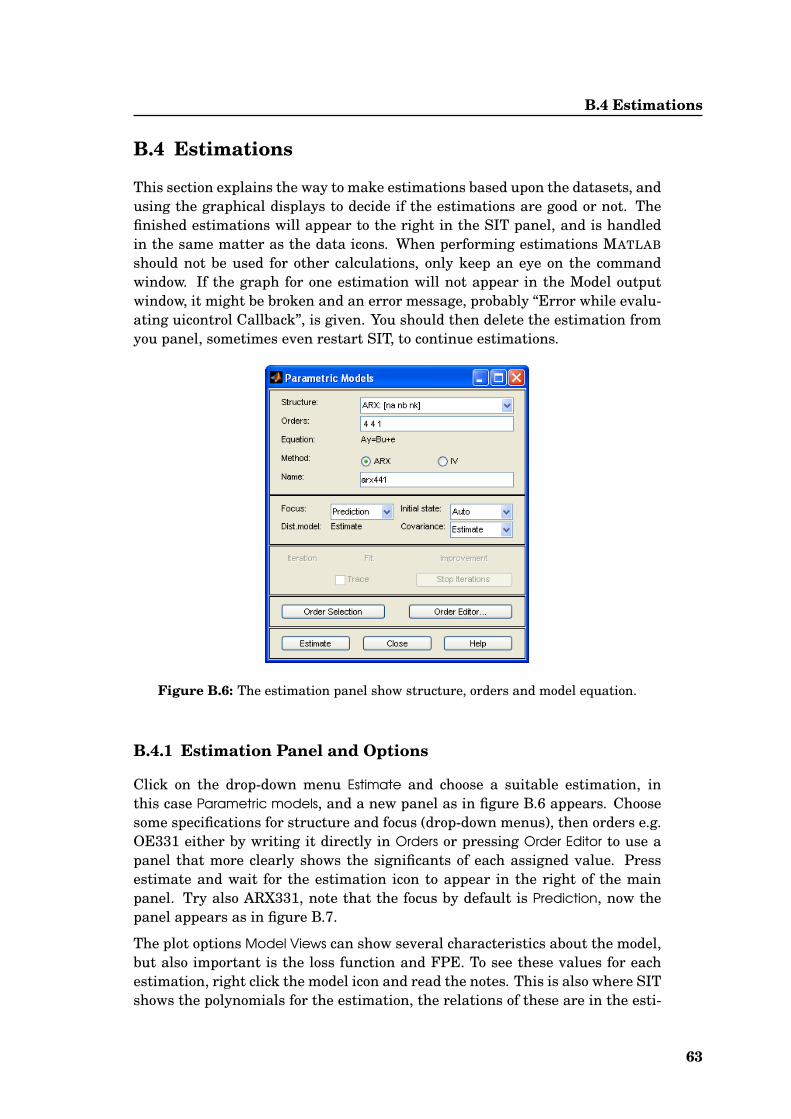
B.4 Estimations
B.4 Estimations
This section explains the way to make estimations based upon the datasets, andusing the graphical displays to decide if the estimations are good or not. Thefinished estimations will appear to the right in the SIT panel, and is handledin the same matter as the data icons. When performing estimations MATLAB
should not be used for other calculations, only keep an eye on the commandwindow. If the graph for one estimation will not appear in the Model outputwindow, it might be broken and an error message, probably “Error while evalu-ating uicontrol Callback”, is given. You should then delete the estimation fromyou panel, sometimes even restart SIT, to continue estimations.
Figure B.6: The estimation panel show structure, orders and model equation.
B.4.1 Estimation Panel and Options
Click on the drop-down menu Estimate and choose a suitable estimation, inthis case Parametric models, and a new panel as in figure B.6 appears. Choosesome specifications for structure and focus (drop-down menus), then orders e.g.OE331 either by writing it directly in Orders or pressing Order Editor to use apanel that more clearly shows the significants of each assigned value. Pressestimate and wait for the estimation icon to appear in the right of the mainpanel. Try also ARX331, note that the focus by default is Prediction, now thepanel appears as in figure B.7.
The plot options Model Views can show several characteristics about the model,but also important is the loss function and FPE. To see these values for eachestimation, right click the model icon and read the notes. This is also where SITshows the polynomials for the estimation, the relations of these are in the esti-
63

“How To” in SIT
mation panel under each structure type. If the error is sufficiently small (lossand FPE are small) it can be ignored and by pressing the Present button in thenote panel, you can move your estimation polynomials from SIT to MATLAB forfurther use. But before you use it you should make sure it is a good estimationso the chance of the model fulfilling the specifications is as high as possible.
Figure B.7: The Model Views can be activated when an estimation is done.
Figure B.8: The estimation polynomials and other proper-ties of the model is found by right-clicking the model icon.
B.4.2 Eliminating Poor Estimations Using Model Views
SIT can show six different graphs for each estimation and you can find the poly-nomials end the error for each of these by right clicking their icon. This sectionadvice how to eliminate estimations and only continue with a few polynomialmodels. The most obvious tool is the best fit window Model output which visu-alize the data put in Validation Data together with all active estimations, and
64

B.4 Estimations
Figure B.9: Model and data output with best fit percentage for the estimations.
to the right shows a percent value that describes how close the estimation is tothe plotted data. See figure figure B.9 above and section B.5.1 on page 68. Theresiduals in Model resids is shown with their 99% confidence interval by defaultbut it is easy to change to 95% under Options or what you find fitting for the es-timations. Preferably lies the graph within these limits the entire range whichcan be expanded by raising the number of lags under Options.
For each estimation the zeros and poles are shown in a z-plan diagram with theunit circle drawn by activating Zeros and poles so the significants of each poleand zero is easily discovered cf. regulation and signals technique. To make surea pole is inside the unit circle zoom in by dragging a zoom square around it. Forresiduals, poles and zeros see figure B.10 below. Furthermore the frequency
Figure B.10: Residuals (mostly) between the limits, and all poles within the circle.
65

“How To” in SIT
response is shown in a Bode plot to investigate closer if needed see Frequencyresp. In this case the frequency response is only regarded to avoid obviously dis-tortion of the estimation, as with Noise spectrum that shows the noise accordingto frequency band, see figure B.11 below. Finally there is the view option Tran-
Figure B.11: Frequency response seems fine and the noise is small since the modelsdo not contain noise parameters.
sient resp where the window has similar options as Model resids. By default thiswindow shows the first little part of a step response and easily shows any irreg-ularities in the first few seconds as in figure B.12 below. Though the range canbe prolonged SIT can do better with the build in LTI viewer.
Figure B.12: At first the response for ARX rises slightly while OE falls
66

B.4 Estimations
B.4.3 Examining Models in LTI Viewer
In the middle of the panel is a box called LTI Viewer and by dropping a modelicon an advanced viewer is launched. Under Edit/Plot Configurations the num-ber of windows and the plot to show in each can be set from 1-6 windows andoptions are among others step and impulse response as shown in this case infigure B.13. This shows that ARX331 falls for approx. 200 seconds and then sta-bilizes, while OE331 quickly falls, then rises and stabilizes all within 2 seconds.Compared to figure B.12 on the preceding page this is a surprise.
The two figures are generated by dropping one model directly in the SIT panelto ”To LTI Viewer” and the other into workspace. The extra viewer comes fromFile/New Viewer and the model from File/Import from workspace. It is also possi-ble to change the color in Edit/Line Styles and preferences in File/Toolbox– or muchthe same in Edit/Viewer–. By double-clicking a graph it is possible to call out anProperty Editor for each graph. By default the axes are set to 90% of the settlingtime, but each axes is controlled under Limits.
By right-clicking in the graph you get some options i.a. plot types as mentionedstep, impulse etc. but also options to show characteristics as settling time, peaketc. The two model step responses shown in figur B.13 are easily compared e.gARX331 is much slower than OE331, settling times being 229 s and 1.3 s, plusthe shapes of the two impulse responses are very different. LTI Viewer can also
Figure B.13: The two models ARX (right) and OE (left) in each a LTI viewer.
make a more detailed Bode plot or Pole-Zero and generate Nichols, Nyquist andseveral more. This is a very strong tool to determine whether or not to continuewith a model, since it easily shows how fast the model is, and how it responsesin general cf. regulation techniques.
67

“How To” in SIT
B.5 Validating Models
In this section you should try and compare the models that was not discardedduring the above with new datasets, preferably from a new line of measure-ments or simulations. The goal is to see how the models fit the system underidentification when under the influence of other actions or at another time.
Figure B.14: Dataset startdata imported and prepared by removing mean beforeuse for validation by dragging to Validation Data.
B.5.1 Working With Several Datasets
Import a new dataset, in this case from the start of the simulation. Prepare it bydragging it to the working box and remove the means, creating the dataset start-datad. Drag it to Validation Data and the panel will now look like figure B.14above.
By activating both meandata and startdatad the datasets is easily compared inthe time plot as in figure B.15. In figure B.16 the two models are now shown inrelation to the new dataset, and by changing the validation data the residualschange too. The graphs in figure B.16 should be evaluated for likeness withfigure B.9 on page 65.
The number of datasets is easily expanded, depending on the type of system anumber of datasets from various states should be included in the system iden-tification, to ensure the best chances of the model fitting expectations. Also alloptions when estimating should be chosen carefully.
Neither of the two models considered here are very good. The fit for OE331 isgood but the responses are bad due the great overshoot. ARX331 has a bad fitand is rather slow, while if estimated with the focus ”Simulation” at can becomemuch better.
When the model is done and you right-click to press Present, note the variationswritten in parenthesis in MATLAB window. They should be rather small or the
68

B.5 Validating Models
Figure B.15: startdatad (gray) has less oscillation than meandata (red).
Figure B.16: The two models compared with the new dataset gives out new fit per-centages.
behavior shown in SIT can change drastically when removing the deviation,these numbers represent. Next is a summery of the preceding pages, as a checklist or reminder when performing the entire estimation from ident to Present.
69
“How To” in SIT
B.6 SIT Summary
This section ends the ”How To” and summarizes the steps done in SIT to per-form system identification on datasets. It is how SIT has been used in thisparticularly project, and in other cases it might not be necessarily or sufficientto carry out the steps below. To know when to perform which step a flow chartmay be useful as in Appendix A.2.
Datasets
• Make a proper measurement or simulation and store the data in a properform e.g. a .txt file.
• Load the dataset correct in SIT.
• Prepare the dataset with the Preprocesses and view it with Data Views.
• Activate the correct dataset in Working data and Validation Data
Now all estimations are performed, while the considerations below is regarded.Before estimating you should consider some properties about the model; blackbox, output-error, state-space etc.
Choosing Estimations
• View the best fit window with the estimations and datasets of your choice.Use the percentage or your eye (zoom in) to decide whether the fit is suit-able.
• Consider the polynomials, the loss function and FPE to see if the model isusable. The values should be as low as possible, often much lesser than 1.
• Use the residuals to judge the nature of loss and FPE. If both are poor youshould consider performing a new estimation.
• Investigate the poles and zeros of the model to make sure they are placedwithin acceptable limits. Beware of especially poles near the unit circle.
• Drag the models to the LTI viewer to investigate the response, e.g. stepand impulse to gain knowledge about the models behavior such as riseand settling time.
• When only a few good models are left, compare to another dataset in Modeloutput and evaluate the result.
When the use of SIT is done, present the wanted model(s) or drag to workspace.Remember to consider the structure equation the model is based upon, whenfurther calculations with the model is executed. Also slight deviation can beexpected between the model in SIT and the presented data due to round off, soa new investigation in MATLAB is a very good idea.
70

Appendix CIllustrations From SIT
Figure C.1: Estimation Various as the panel appears; all models based on meandata.
Figure C.2: Estimations ARX as the panel appears; all models based on data1088d
71

Illustrations From SIT
(a) (b)
Figure C.3: (a) The noise from the most noisy models; ARX10108(sandy), -552(violet), -431(orange), -982(red), -873(light blue), -551(dark blue) and the lone oneis BJ22221(dark brown).(b) The noise from the two best ARX models; -331(blue) & -341(turquoise) and OE ontop of each other; -331(green) & -341(dark green)
(a) (b)
Figure C.4: (a) The residuals for all of these models are practically the same.(b) Only by zooming in it is reviled that the ARMAX(gray) has poorer residuals
72

Figure C.5: The cross correlations is the important residual for OE, so the limithas been raised to 95%. To the right all OE and BJ; OE321(pink), OE431(lilac) andBJ2221(dark brown) have poor residuals. To the left the two best OE331 & OE221
(a) (b)
Figure C.6: (a) The frequency responses for all that look suspicious. ClearlyARX331(yellow) is unstable and OE431(lilac), ARX552(violet) ARX10108(sandy) prob-ably too. ARX551(dark blue) showed instability earlier so the rest except for ARX andOE 331 should be closely examined since their appear similar.OE331(green) appears similar to ARX431(orange) which has very poor fit and is likelyunstable. This calls for further investigation.(b) Frequency response for the four best as above.
73
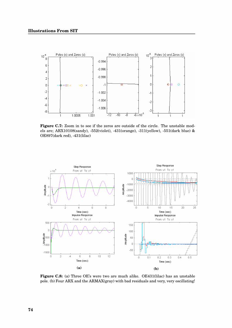
Illustrations From SIT
Figure C.7: Zoom in to see if the zeros are outside of the circle. The unstable mod-els are; ARX10108(sandy), -552(violet), -431(orange), -311(yellow), -551(dark blue) &OE897(dark red), -431(lilac)
(a) (b)
Figure C.8: (a) Three OE’s were two are much alike. OE431(lilac) has an unstablepole. (b) Four ARX and the ARMAX(gray) with bad residuals and very, very oscillating!
74

(a) (b)
Figure C.9: (a) Settling times shown for OE; (b) Shape and peaks shown for OE.The two OE models are very much alike, though OE331 has a higher order.
(a) (b)
Figure C.10: (a) Settling times shown for ARX; (b) Shape and peaks shown for ARX.The two ARX are similar but ARX331(blue) is faster.
75

Illustrations From SIT
Figure C.11: The models sorted according to type, fit and behavior. To the left: lilac,dark red, dark brown, light brown, green, dark green, pink. To the right; gray, blue,turquoise, light blue, red, violet, sandy, orange, yellow, dark blue.
(a) Validated against meandata ARX will swing in the first seconds.
(b) According to data1088d the fit actually improves for both models.
(c) The start lowers the fit slightly and ARX swings in again.
Figure C.12: Fit for the two chosen models and the three dataset.
76

(a) Validated against meandata ARX is still good.
(b) OE validated with data1088d gives worse residuals.
(c) The start gives fine residuals for borth models.
Figure C.13: Related residuals for the comparisons.
77


Appendix DModel in Simulink
A simulink model as in figure D.2 on the next page has been made in under-standing the PF system and for investigating the behavior of equations (1.2.1)through (1.2.3) pages 6–7, when the input is the frequency from PF.
The models shows that the heater block consists of two major pats; a differen-tial equation with temperature as control signal and an switch or comparisonpart with frequency as control signal. The power is united output and influ-ences both control signals; the frequency through the electrical net and thetemperature through the room represented by the differential equation.
By modeling the system in Simulink we can investigate the behavior of thesystem with either the data as frequency/power or by fixing the power to a step.
Figure D.1: The temperature T, when the input is the frequency from the original PFmodel, and the power is a step function.
Figure D.1 shows the temperature which controlls the entire system togetherwith the frequency. The single temperature in the figure resembles in shapethe ones PF have 100 of, only it rises a bit faster. A general lower temperaturesetting and a lower power demand go together.
79
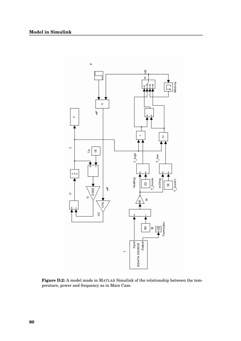
Model in Simulink
Figure D.2: A model made in MATLAB Simulink of the relationship between the tem-perature, power and frequency as in Main Case.
80
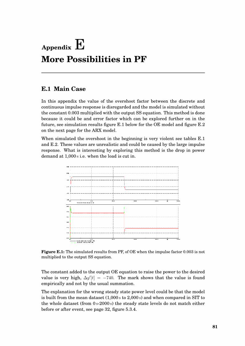
Appendix EMore Possibilities in PF
E.1 Main Case
In this appendix the value of the overshoot factor between the discrete andcontinuous impulse response is disregarded and the model is simulated withoutthe constant 0.003 multiplied with the output SS equation. This method is donebecause it could be and error factor which can be explored further on in thefuture, see simulation results figure E.1 below for the OE model and figure E.2on the next page for the ARX model.
When simulated the overshoot in the beginning is very violent see tables E.1and E.2. These values are unrealistic and could be caused by the large impulseresponse. What is interesting by exploring this method is the drop in powerdemand at 1,000 s i.e. when the load is cut in.
Figure E.1: The simulated results from PF, of OE when the impulse factor 0.003 is notmultiplied to the output SS equation.
The constant added to the output OE equation to raise the power to the desiredvalue is very high, ∆y′[t] = −740. The mark shows that the value is foundempirically and not by the usual summation.
The explanation for the wrong steady state power level could be that the modelis built from the mean dataset (1,000 s to 2,000 s) and when compared in SIT tothe whole dataset (from 0 s-2000 s) the steady state levels do not match eitherbefore or after event, see page 32, figure 5.3.4.
81
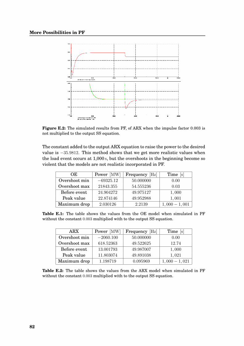
More Possibilities in PF
Figure E.2: The simulated results from PF, of ARX when the impulse factor 0.003 isnot multiplied to the output SS equation.
The constant added to the output ARX equation to raise the power to the desiredvalue is −35.9812. This method shows that we get more realistic values whenthe load event occurs at 1,000 s, but the overshoots in the beginning become soviolent that the models are not realistic incorporated in PF.
OE Power [MW] Frequency [Hz] Time [s]Overshoot min −69325.12 50.000000 0.00Overshoot max 21843.355 54.555236 0.03
Before event 24.904272 49.975127 1, 000Peak value 22.874146 49.952988 1, 001
Maximum drop 2.030126 2.2139 1, 000− 1, 001
Table E.1: The table shows the values from the OE model when simulated in PFwithout the constant 0.003 multiplied with to the output SS equation.
ARX Power [MW] Frequency [Hz] Time [s]Overshoot min −2060.100 50.000000 0.00Overshoot max 618.52363 49.522625 12.74
Before event 13.001793 49.987007 1, 000Peak value 11.803074 49.891038 1, 021
Maximum drop 1.198719 0.095969 1, 000− 1, 021
Table E.2: The table shows the values from the ARX model when simulated in PFwithout the constant 0.003 multiplied with to the output SS equation.
82
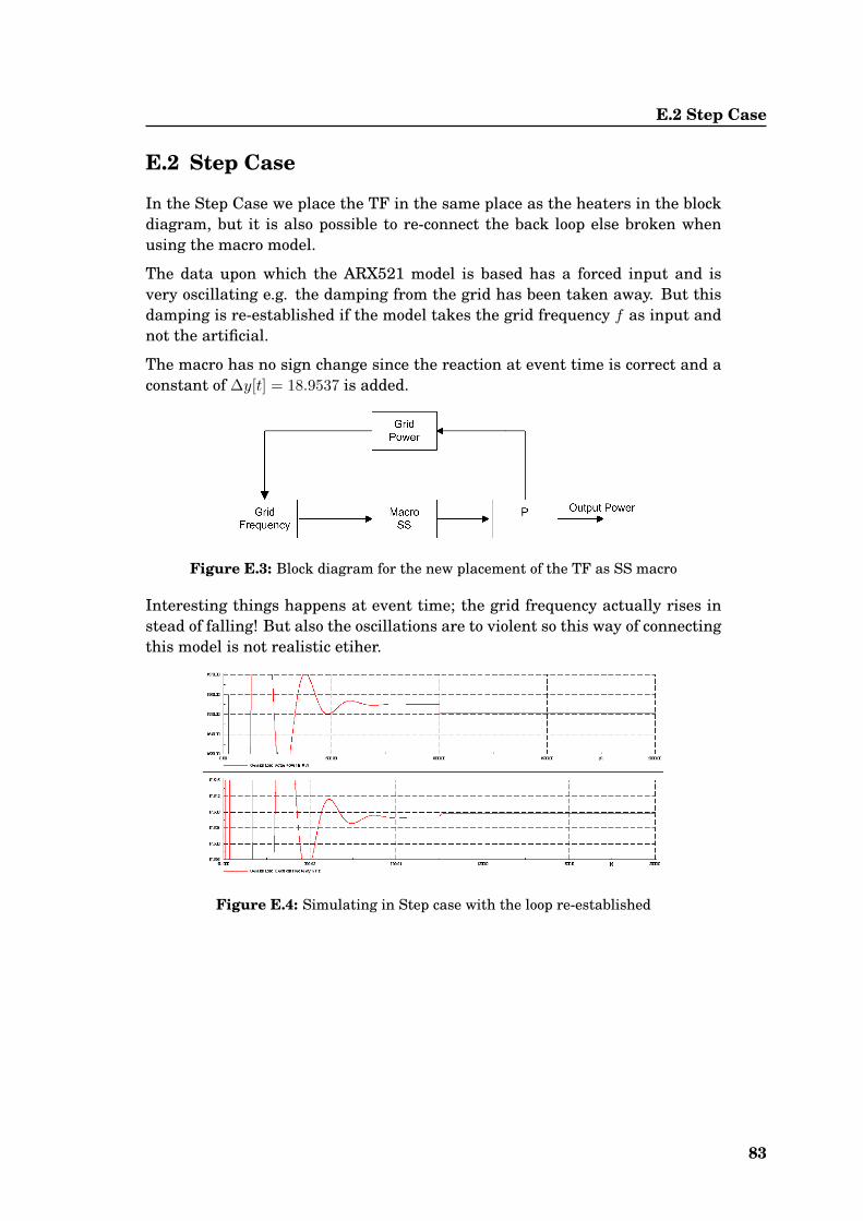
E.2 Step Case
E.2 Step Case
In the Step Case we place the TF in the same place as the heaters in the blockdiagram, but it is also possible to re-connect the back loop else broken whenusing the macro model.
The data upon which the ARX521 model is based has a forced input and isvery oscillating e.g. the damping from the grid has been taken away. But thisdamping is re-established if the model takes the grid frequency f as input andnot the artificial.
The macro has no sign change since the reaction at event time is correct and aconstant of ∆y[t] = 18.9537 is added.
Figure E.3: Block diagram for the new placement of the TF as SS macro
Interesting things happens at event time; the grid frequency actually rises instead of falling! But also the oscillations are to violent so this way of connectingthis model is not realistic etiher.
Figure E.4: Simulating in Step case with the loop re-established
83


www.oersted.dtu.dk/cet
Ørsted • DTUCentre for Electric Technology (CET)Technical University of DenmarkElektrovej 325DK-2800 Kgs. LyngbyDenmarkTel: (+45) 45 25 35 00Fax: (+45) 45 88 61 11E-mail: [email protected]