Embed Size (px)
Citation preview
THESIS FOR THE DEGREE OF DOCTOR OF PHILOSOPHY
DEM Modelling and Simulation of Cone Crushers and
High Pressure Grinding Rolls
JOHANNES C.E. QUIST
Department of Product and Production Development
CHALMERS UNIVERSITY OF TECHNOLOGY
Gothenburg, Sweden 2017

DEM Modelling and Simulation of Cone Crushers and High Pressure Grinding Rolls
JOHANNES C.E. QUIST
Copyright 2017 © JOHANNES C.E. QUIST
Doktorsavhandlingar vid Chalmers tekniska högskola
ISSN 0346-718-4225
ISBN 978-91-7597-544-3
Department of Product and Production Development
Chalmers University of Technology
SE-412 96 Gothenburg
Sweden
Telephone + 46 (0)31-772 1000
URL www.chalmers.se/
Cover:
Illustration of DEM-particles being crushed
Chalmers Reproservice
Gothenburg, Sweden 2017

“Everything develops through the mechanism of iteration”

i
Abstract
The comminution of rock and ore materials consumes ~1.5-1.8 % of the total energy production
in mining intensive countries (Tromans, 2008). Several research findings show that there are ways
of utilizing compressive breakage modes that are more energy efficient compared to conventional
grinding circuits based on large inefficient tumbling mills. Circuits using Cone Crushers and
High Pressure Grinding Rolls (HPGR) have proven to be more energy efficient. These
comminution devices have during the last two decades been implemented for hard rock
materials. These machines are hence suitable subjects for further performance improvement and
optimization.
In this thesis a simulation platform, based on the Discrete Element Method (DEM), for simulation
of compressive breakage machines such as Cone Crushers and HPGRs is presented. The research
notion is that in order to further develop compressive breakage machines and operations,
fundamental understanding is needed with regard to specific details inside the machines.
The rock particles are modelled using the Bonded Particle Model (BPM) and particle shapes are
based on 3D scanned rocks. The machine geometry is based on CAD modelling and 3D scanning.
The interactions between rock particles and between rock particles and the machine boundaries
are modelled using contact models that determine the reaction forces. A novel DEM calibration
and validation framework based on design of experiments, surrogate modelling and multi-
objective optimization has been developed for calibrating and validating particle flow and
breakage.
Seven different simulation case studies are included in the thesis work. The simulation and
modelling capabilities have successively progressed for each study conducted. The result and
findings are both attributed to machine specific insights and generic modelling findings.
The work shows that the most vital machine and process performance responses, such as product
size distribution, pressure distributions and power draw can be predicted using the DEM
simulation platform.
ii
Sammanfattning
Krossning och sönderdelning av berg- och malmmaterial förbrukar ~ 1.5-1.8% av den totala
energiproduktionen i gruvintensiva länder (Tromans, 2008). Ett flertal studier har visat att man
genom att utnyttja kompressiv krossning kan uppnå mer energieffektiva lösningar jämfört med
konventionella malprocesser baserade på stora tumlande kvarnar. Processer baserade på
användning av konkrossar och HPGR maskiner (High Pressure Grinding Rolls) har visat sig vara
mer energieffektiva. Dessa maskiner är därför lämpliga kandidater för ytterligare
prestandaförbättringar och optimering.
I denna avhandling presenteras en simuleringsplattform, baserad på diskret elementmetod
(DEM), för simulering av kompressiv krossmaskiner. Ett grundläggande antagande för
forskningen är att ytterligare förståelse och kunskap angående maskinernas inre mekanismer är
nödvändig för att möjliggöra fortsatt vidareutveckling samt kostnadseffektiv utveckling av nya
maskiner.
I simuleringsmiljön modelleras bergmaterialpartiklar genom användning av en Bunden Partikel
Modell (BPM). Modeller för maskingeometri skapas genom CAD-modellering samt i vissa fall
3D-scanning. Interaktionen mellan enskilda partiklar samt mellan partiklar och maskingeometri
kontrolleras genom så kallade kontaktmodeller. För att åstadkomma god överenstämmelse
mellan simulering och verklig process krävs kalibrering och validering av dessa kontaktmodeller.
En ny utrustning samt metodik för kalibrering har i projektet utvecklats baserat på
flödesexperiment, statistisk försöksplanering, surrogat modellering samt optimering.
Totalt sju olika simuleringsfallstudier är beskrivna i avhandlingen, där simulerings och
modelleringsfunktioner successivt har utvecklats för varje studie. De resultat och insikter som
gjorts i dessa studier är både relaterade till maskinspecifika lärdomar samt ny förståelse gällande
DEM simulering och modellering.
Arbetet visar att de mest vitala processtekniska maskinparametrarna, såsom
produktstorleksfördelning, tryckrespons och effektuttag kan förutsägas med hjälp av
simuleringsplattformen.
iii
Publications
The thesis contains the following papers:
Paper A: Quist, J., Evertsson, C. M., Simulating Capacity and Breakage in Cone
Crushers Using DEM, 7th International Comminution Symposium
(Comminution '10). 2010: Cape Town, South Africa.
Paper B: Quist, J., Evertsson, C. M., Application of discrete element method for
simulating feeding conditions and size reduction in cone crushers. in XXV
International Mineral Processing Congress. 2010. Brisbane, Australia.
Paper C: Quist, J., Evertsson, C. M., Franke, J., The effect of liner wear on gyratory
crushing – a DEM case study, 3rd International Computational Modelling
Symposium (Computational Modelling '11). 2011: Falmouth.
Paper D: Quist, J., Evertsson, C. M., Simulating Pressure Distribution in HPGR using
the Discrete Element Method, 8th International Comminution Symposium
(Comminution '12). 2012: Cape Town.
Paper E: Quist, J., Evertsson, C. M., Simulating breakage and hydro-mechanical
dynamics in high pressure grinding rolls using the discrete element method, in
ESCC 2013 (European Symposium on Comminution & Classification).
2013. p. 209-2012.
Paper F: Quist, J., Evertsson, C. M., Calibration of DEM Contact Models, Submitted to
Granular Matters, Feb 2017
Paper G: Quist, J., Evertsson, C. M., Cone Crusher modelling and simulation using
DEM, Minerals Engineering , 2016
Paper H: Johansson, M., Quist, J., Evertsson, C. M., Hulthén, E., Cone crusher
performance evaluation using DEM simulations and laboratory experiments for
model validation, Minerals Engineering, 2016
Paper I: Quist, J., Johansson, M., Evertsson, C. M., Calibration of DEM Bonded
Particle Model Using Surrogate Based Optimization, Under review for
Minerals Engineering
Paper J: Quist, J., Evertsson, C. M, Investigation of Roller Pressure and Shear Stress
in the HPGR using DEM, in XXVIII International Mineral Processing
Congress, 2016: Quebec, Canada
In papers A-G and J, Quist and Evertsson initiated the idea. The implementation was performed by
Quist. Quist wrote the paper with Evertsson as a reviewer.
In paper H, Quist, Johansson and Evertsson initiated the idea. M. Johansson and Quist performed the
DEM modelling and co-wrote the paper with Evertsson and Hulthén as a reviewers.
In paper I, Quist initiated the idea. Quist and Johansson performed the DEM modelling and experiments
and co-wrote the paper with Evertsson as reviewer.

iv
Other publications
Weerasekara, N. S., Powell, M. S., Cleary, P. W., Tavares, L. M., Evertsson, C. M., Morrison, R. D., Quist, J.,
Carvalho, R. M. (2013). The contribution of DEM to the science of comminution. Powder
Technology, 248(0), 3-24. doi:http://dx.doi.org/10.1016/j.powtec.2013.05.032
Evertsson, C. M., Hulthén, E., Bengtsson, M., Quist, J. (2014) Control systems for improvement of cone
crusher yield and operation. Proceedings of Comminution '14.
Quist, J., Evertsson, C. M. (2015) Framework for DEM Model Calibration and Validation . Proceedings of
the 14th European Symposium on Comminution and Classification (ESCC 2015). 7-11
September 2015, Gothenburg, Chalmers University s. 103-108.
Quist, J., Evertsson, C.M. (2015) Poly-stream Comminution Circuits, Proceedings of the 14th European
Symposium on Comminution and Classification (ESCC 2015). 7-11 September 2015,
Gothenburg, Chalmers University s. 103-108.
Evertsson, C.M., Quist, J., Bengtsson, M., Hulthén, Erik (2016), Monitoring and validation of life time
prediction of cone crusher with respect to loading and feeding conditions. Comminution 16. 904
(1 Vol) ISBN 9781510826670
v
Contents
Abstract ........................................................................................................................................................ i
Sammanfattning......................................................................................................................................... ii
Publications ...............................................................................................................................................iii
Contents ...................................................................................................................................................... v
Preface ...................................................................................................................................................... vii
Notation .................................................................................................................................................. viii
1 Introduction ....................................................................................................................................... 1
1.1 Industrial Challenges ............................................................................................................... 4
2 Research Approach ........................................................................................................................... 7
2.1 Research Questions .................................................................................................................. 7
2.2 Delimitations ............................................................................................................................ 7
2.3 Scientific Approach .................................................................................................................. 8
3 Background ........................................................................................................................................ 9
3.1 Minerals Processing ................................................................................................................. 9
3.2 Cone Crushers .......................................................................................................................... 9
3.3 High Pressure Grinding Rolls .............................................................................................. 11
3.4 Compressive Breakage .......................................................................................................... 12
4 Discrete Element Method ............................................................................................................... 15
4.1 Equations of Motion .............................................................................................................. 16
4.2 Numerical Integration ........................................................................................................... 16
4.3 Rotation of Particles ............................................................................................................... 18
4.4 Contact Detection ................................................................................................................... 18
4.5 Contact Kinematics ................................................................................................................ 19
4.6 Hertz-Mindlin Contact Model .............................................................................................. 20
4.7 Shape Representation ............................................................................................................ 22
4.8 Breakage Models .................................................................................................................... 23
4.9 Bonded Particle Model .......................................................................................................... 25
4.10 Rock-Shaped Meta-Particles ................................................................................................. 27
5 Simulation Based Design ............................................................................................................... 31
5.1 Example: Cone Crusher Feeding Problem.......................................................................... 33
5.2 Example: Development of Cone Crusher Liner Design.................................................... 33
6 Verification and Validation ........................................................................................................... 35
6.1 Surrogate Modelling .............................................................................................................. 37
6.2 Polynomial Regression .......................................................................................................... 39
6.3 General Model Calibration ................................................................................................... 40
vi
6.4 Error Measures ....................................................................................................................... 41
6.5 Calibration Optimization Formulation ............................................................................... 42
6.6 Bonded Particle Model Calibration ..................................................................................... 44
6.7 Particle Flow Calibration ...................................................................................................... 49
6.8 Calibration Device ................................................................................................................. 49
7 Cone Crusher Modelling ................................................................................................................ 55
7.1 Cone Crusher Eccentric Speed ............................................................................................. 55
7.2 Primary Gyratory Crusher - Influence of Liner Wear ....................................................... 57
7.3 Cone Crusher Close Side Setting ......................................................................................... 59
8 HPGR Modelling ............................................................................................................................. 63
8.1 Roller Pressure Distribution ................................................................................................. 63
8.2 Modelling Dynamics ............................................................................................................. 68
8.3 Investigation of Dynamics, Shear and Pressure Profile .................................................... 71
9 Discussion and Conclusions .......................................................................................................... 75
9.1 General Conclusions .............................................................................................................. 76
9.2 Answering Research Questions ........................................................................................... 76
9.3 Scientific Contribution ........................................................................................................... 77
9.4 Vision for further development ........................................................................................... 79
10 References ........................................................................................................................................ 81
Appended papers
Paper A: Simulating Capacity and Breakage in Cone Crushers Using DEM
Paper B: Application of discrete element method for simulating feeding conditions and size
reduction in cone crushers
Paper C: The effect of liner wear on gyratory crushing – a DEM case study
Paper D: Simulating Pressure Distribution in HPGR using the Discrete Element Method
Paper E Simulating breakage and hydro-mechanical dynamics in high pressure grinding
rolls using the discrete element method
Paper F: Calibration of DEM Contact Models
Paper G: Cone Crusher modelling and simulation using DEM
Paper H: Cone crusher performance evaluation using DEM simulations and laboratory
experiments for model validation
Paper J: Calibration of DEM Bonded Particle Model Using Surrogate Based Optimization
Paper I: Investigation of Roller Pressure and Shear Stress in the HPGR using DEM
vii
Preface
The research presented in this thesis was carried out at the research group Chalmers Rock
Processing Systems at the department of Product and Production Development, Chalmers
University of Technology. The research project has received support from the Sustainable
Production Initiative - Production Area of Advance and from Ellen, Walter and Lennart
Hesselmans foundation for scientific research. Without this support the project would not have
been possible and it is gratefully acknowledged.
I would first like to thank my supervisor Professor Magnus Evertsson. It has been a great journey
so far and it is a privilege working with you. I am very thankful for your sharing of expertise, and
sincere and valuable guidance and encouragement. Many thanks also to my co-supervisor Dr.
Erik Hulthén for always finding time to discuss both details and holistic perspectives with great
enthusiasm and clarity.
Additionally, I would like to take this opportunity to express my gratitude to all past and present
members of the CRPS research group and department faculty members for sharing expertise,
guidance and all the valuable and senseless conversations.
Furthermore, I would like to express my gratitude to the fantastic members of our research group
that I have had the pleasure of working with including Dr. Gauti Asbjörnsson, Dr. Magnus
Bengtsson, Rebecka Stomvall, Anton Hjalmarsson, Josefine Berntsson, Dr. Robert Johansson, Dr.
Elisabeth Lee, Ali Davoodi, Simon Grunditz, Lorena Guldris Leon and Marcus Mårlind. I have to
express a very special gratitude towards Marcus Johansson and Albin Gröndahl for your hard
work and patience. At MinFo – Swedish Mineral Processing Research Association I would like to
thank Jan Bida. Also, thank you all fellow colleagues at the Global Comminution Collaborative
(GCC). The support from the team at DEM-Solutions Ltd and the EDEM academic program is
also greatly acknowledged.
Finally I would like to thank my dad Gunno, mom Anna-Lena, my sisters Helena, Malin and
Hanna for all the love, care and great support and especially my girlfriend Cecilia for always
being there with all your motivation, inspiration and love.
Johannes Quist
Göteborg, April 2017
viii
Notation
AG Autogenous Grinding
ANOVA Analysis of Variance
BEM Boundary Element Model
BPM Bonded Particle Model
CAE Computer Aided Engineering
CSS Close Side Setting
CCD Central Composite Design
DEM Discrete Element Method
DOE Design of Experiments
FEM Finite Element Method
HMNS Hertz-Mindlin No Slip Model
HPGR High Pressure Grinding Roll
IPB Inter-Particle Breakage
MOO Multi-Objective Optimisation
PBRM Population Balance Replacement Model
SAG Semi-Autogenous Grinding
SPB Single Particle Breakage
PEM Polyhedral Element Model
im Mass of particle i
if Interaction force
iT Interaction torque
ix Position vector, particle i
iv Velocity vector, particle i
i Angular velocity vector, particle i
iI Moment of inertia, particle i g Gravitational field constant
h Euler time-step
n Normal unit vector
t Tangential unit vector
n Normal interaction overlap
t Tangential interaction overlap
iR Radius of particle i
,i cr Local contact position vector
,rel cv Relative contact point velocity vector
nF Normal contact force vector
ix
d
nF Normal contact damping force vector
E Equivalent Young’s modulus n
jiv Normal relative contact velocity n
jiv Tangential relative contact velocity
Damping constant
nk Normal contact stiffness
i Poisson’s ratio
e Coefficient of restitution
s Coefficient of static friction
r Coefficient of rolling friction
bF Bond resultant force
,n bF Bond normal force
,n bF Bond tangential force n
bM Bond normal moment s
bM Bond shear moment n
bk Bond normal stiffness s
bk Bond shear stiffness
n Normal angular overlap
t Tangential angular overlap
c Critical normal stress constraint
c Critical shear stress constraint
y Prediction function
Vandermonde matrix
j Error deviation constraint
Error estimate
x Optimization design variable vector g Inequality constraints
h Equality constraints p Parameters
Variable set constraint
jw Objective function weight constant
i Roller angular position
m Mass flow rate
R Roller radius
b Roller width
0v Particle bed initial velocity
1,2T Left and right roller torque

DEM MODELLING AND SIMULATION OF CONE CRUSHERS AND HIGH PRESSURE GRINDING ROLLS
1
1 Introduction
Computer simulations have been used since the late WWII years to understand complex systems
that are not possible to solve using only analytical closed form expressions. The two
mathematicians Jon von Neumann and Stanislaw Ulam realised during the years 1946-47 that
computers could be used for implementing a statistical approach to problems related to neutron
diffusion and other questions of mathematical physics (Eckhardt, 1987). This idea spawned into
becoming the Monte Carlo method and the era of modelling and simulation using computers was
born.
Since then, simulation methods have become increasingly important for scientists to better
understand the world and for engineers in their efforts of designing machines and processes.
Today many industries heavily depend on simulations as virtual environments for testing
concepts and principles before creating any physical objects or prototypes. This reduces the need
for physical prototypes and experiments which leads to decreased development costs and lower
risks. However, the risk and cost reduction is dependent on that the simulation results conform
to reality within the domain under study. Calibration and validation of models are therefore of
utmost importance if decisions are to be made based on simulation outcomes.
This thesis work targets discrete element modelling and simulation (DEM) of the comminution
of rock and ore materials in two different machines used in the minerals processing industry. The
research project is named Optimal Crushing and Grinding and is conducted within the research
group Chalmers Rock Processing Systems (CRPS) at Chalmers University of Technology,
Sweden.
Comminution is the process in which ore particles are broken and reduced in size to a level where
the minerals of interest can be separated, or in other words liberated from the waste gangue rock.
The size reduction is done in sequential steps through a series of comminution, classification and
separation stages. The choice of circuit design is governed by several factors including ore type
and grade, ore deposit variability, scale of operation, company culture and available capital
investment.
Schönert (1972; 1979) stated that the compression of single particles between two plates is a
suitable benchmark experiment in order to evaluate the breakage efficiency in comminution. As
reported in the study by Fuerstenau (2002) there are controlled laboratory particle cleavage tests
that are capable of achieving breakage efficiencies above 1.0 m2/J. In comparison the Schönert
compression tests showed a breakage efficiency of 0.02 m2/J and the Hukki (1944) experiments
using a pendulum crusher resulted in 0.01 m2/J. However, when comparing these values with
ball milling experiments reported in the Fuerstenau study, with an efficiency of ~0.0028 m2/J, it is
clear that the compression breakage mode requires less energy to produce the same amount of
JOHANNES QUIST
2
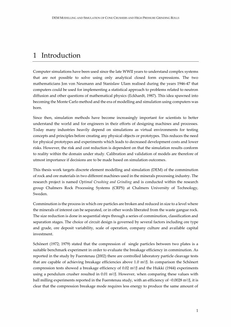
new surface area. The efficiency and breakage probability can be directly linked to the number of
contact points per particle and hence the stress concentration level for each contact point given a
certain force level applied. An illustration of different particle loading conditions can be seen in
Figure 1.
Figure 1. Schematic illustration of particle breakage crack patterns for four different loading
conditions a) Impact particle breakage b) Point contact loading on a particle supported by a soft
compression plate c) Two-point contact loading d) Multiple-point contact loading. (modified from
(Schönert, 1979)).
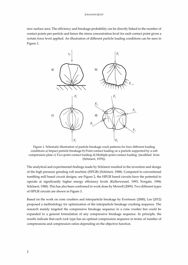
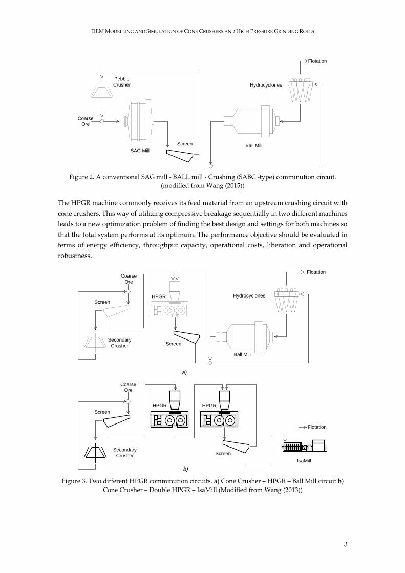
The analytical and experimental findings made by Schönert resulted in the invention and design
of the high pressure grinding roll machine (HPGR) (Schönert, 1988). Compared to conventional
tumbling mill based circuit designs, see Figure 2, the HPGR based circuits have the potential to
operate at significantly higher energy efficiency levels (Kellerwessel, 1993; Norgate, 1994;
Schönert, 1988). This has also been confirmed in work done by Morrell (2009). Two different types
of HPGR circuits are shown in Figure 3.
Based on the work on cone crushers and interparticle breakage by Evertsson (2000), Lee (2012)
proposed a methodology for optimization of the interparticle breakage crushing sequence. The
research mainly targeted the compressive breakage sequence in a cone crusher but could be
expanded to a general formulation of any compressive breakage sequence. In principle, the
results indicate that each rock type has an optimal compression sequence in terms of number of
compressions and compression ratios depending on the objective function.
0v
a) b)
c) d)
1F
2F
3F
4F
5F
6F
i nF
1F
1F
2F
DEM MODELLING AND SIMULATION OF CONE CRUSHERS AND HIGH PRESSURE GRINDING ROLLS
3
Figure 2. A conventional SAG mill - BALL mill - Crushing (SABC -type) comminution circuit.
(modified from Wang (2015))
The HPGR machine commonly receives its feed material from an upstream crushing circuit with
cone crushers. This way of utilizing compressive breakage sequentially in two different machines
leads to a new optimization problem of finding the best design and settings for both machines so
that the total system performs at its optimum. The performance objective should be evaluated in
terms of energy efficiency, throughput capacity, operational costs, liberation and operational
robustness.
Figure 3. Two different HPGR comminution circuits. a) Cone Crusher – HPGR – Ball Mill circuit b)
Cone Crusher – Double HPGR – IsaMill (Modified from Wang (2013))
Coarse
Ore
Pebble
Crusher
SAG MillBall Mill
Hydrocyclones
Flotation
Screen
Coarse
Ore
Secondary
Crusher
Screen
Screen
Ball Mill
HydrocyclonesHPGR
Flotation
Coarse
Ore
Secondary
Crusher
Screen
HPGR
Screen
HPGR
Flotation
IsaMill
a)
b)
JOHANNES QUIST
4
The simulation platform is based on the discrete element method (DEM) originally proposed by
Cundall (1971; 1979). Since proposed, the method has been developed into the most powerful
methodology for simulating particle flow and breakage. A thorough portrayal of how DEM has
been utilized within the research field of comminution has been presented by Weerasekara et al.
(2013).
As a part of the development of the simulation platform the cone crusher and the HPGR have
been modelled and investigated. The presented results are hence both related to new knowledge
in the research field of DEM as well as in the research field of crushing and comminution.
1.1 Industrial Challenges
The mining and minerals industries are facing a series of challenges related to fluctuating market
demands, business competition and environmental constraints with the continuous need for new
technology and innovation as a consequence. What is regarded as a technology challenge will
differ from country to country and between minerals processing operations. However, four major
trends that have been identified and could be regarded as general are listed below:
Market demand for commodities and metals increases globally
The ore grade is generally decreasing since most easily accessible ore deposits have
already been exploited
The ore material competence is generally higher as material is mined at greater depth
where weathering effects are less likely to have affected the ore over time
Due to reduced grade, larger masses of fresh ore need to be processed in order to produce
the same amount of finished product
Summarizing the four listed challenges leads to the conclusion that, if the technology is not
changed, energy consumption will have to be increased in order to keep operations at the same
levels. The energy consumption used by comminution processes in USA, Canada, Australia and
South Africa have been investigated by Tromans (2008). The estimated energy consumption
related to comminution was between ~1.5-1.8 % of the total energy usage in the mentioned
countries (based on governmental statistical data from 2004-2006). This is a significant portion of
the total energy usage and the logical consequence of the three above mentioned challenges is
that the energy demand will increase without further development and implementation of new
technology.
Minimizing the energy demand in comminution operations could be achieved by:
1. Making existing machines more effective within the processes where they currently
operate.
2. Optimizing existing machine concepts with geometrical alternations, sensor technology
and control.
3. Developing novel machine concepts or hybrid solutions.
4. Total transformation of comminution circuit designs i.e. technology quantum leap

DEM MODELLING AND SIMULATION OF CONE CRUSHERS AND HIGH PRESSURE GRINDING ROLLS
5
All four of these activities require engineering design and innovation in order to be realised
in action. It is unlikely that a major new breakthrough will be possible without new
engineering methodologies, providing the capacity of achieving more accurate and less
expensive predictions of not yet materialised concepts of machines and processes. Therefore,
the notion of this thesis is that a virtual simulation environment is needed so that existing
and novel comminution equipment, such as rock crushers, can be tested and understood on
a fundamentally new level.

JOHANNES QUIST
6
DEM MODELLING AND SIMULATION OF CONE CRUSHERS AND HIGH PRESSURE GRINDING ROLLS
7
2 Research Approach
The objective of this work is to develop a virtual platform for evaluating the performance of
compressive breakage machines. The platform can be used for gaining fundamental
understanding and optimization as well as evaluation of novel comminution concepts.
In order for the simulation platform to be of any value in the research and development decision
making process, the results need to be trustworthy. Hence the development of validation and
calibration methods is an integral part of the work.
2.1 Research Questions
A set of research questions have been formulated with the purpose of guiding the research
process. The focus of the research questions varies from modelling specific to more holistic
development perspectives.
RQ.1 How should DEM be used to understand and diagnose operating equipment in
comminution processes?
RQ.2 How should DEM be used as a design evaluation tool in a product development
context?
RQ.3 How should rock breakage in compressive breakage machines be modelled in order to
balance validity and computational economy?
RQ.4 What is a suitable method for calculating the particle size distribution of a bonded
particle model?
RQ.5 How should DEM material models be calibrated with regards to particle flow?
RQ.6 How should DEM material models be calibrated with regards to particle breakage?
RQ.7 How should machine geometry be modelled in DEM?
RQ.8 How should machine dynamics be integrated with DEM?
RQ.9 How should the estimation of forces, pressure and power draw be conducted?
RQ.10 How should DEM simulations be validated?
2.2 Delimitations
To limit the scope of the research a set of delimitations have been formulated as listed below:
Commercial and/or open source software will be used. No software will be developed,
because of time constraints.
Classification and separation machines or operations will not be simulated or studied in
detail
JOHANNES QUIST
8
2.3 Scientific Approach
This work has been carried out at the Chalmers Rock Processing Systems (CRPS) research group
at the department of Product and Production Development. The background of the group is
within the field of machine elements and machine design. The philosophical foundation of the
research is that optimization and improvement of machine design can be achieved by
fundamental understanding of the components and machines studied. The research process can
further on be described as problem oriented. The problem oriented research approach has been
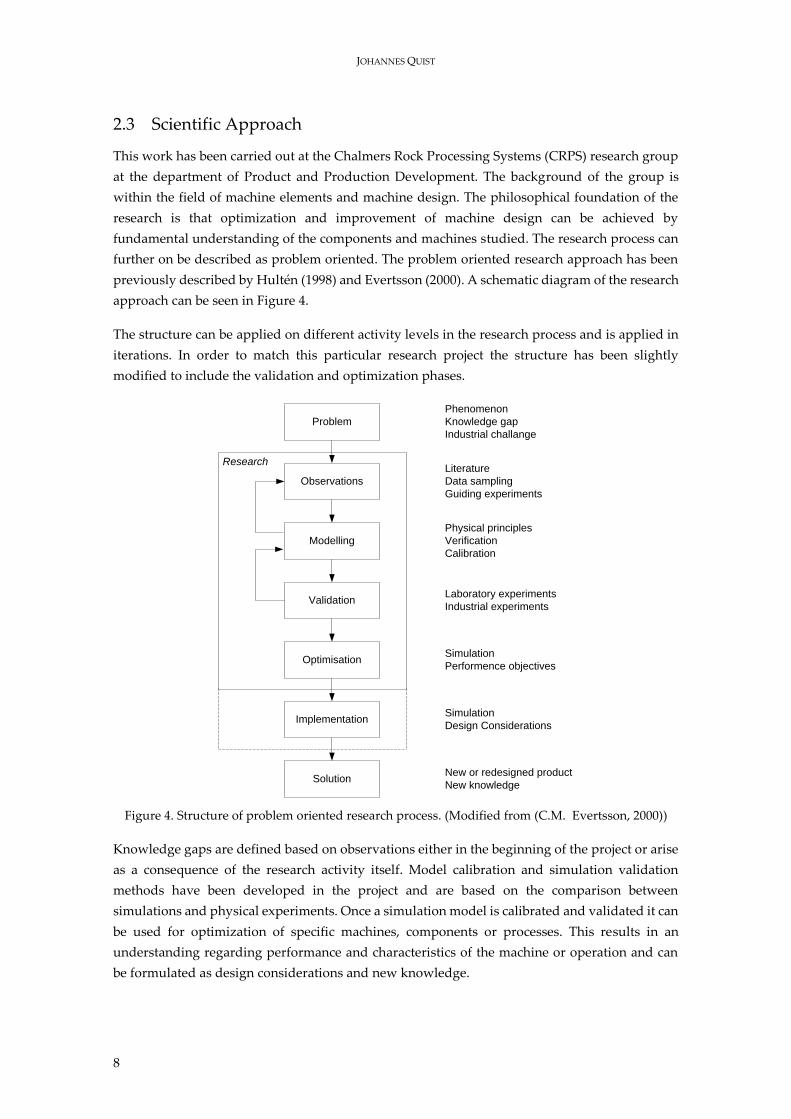
previously described by Hultén (1998) and Evertsson (2000). A schematic diagram of the research
approach can be seen in Figure 4.
The structure can be applied on different activity levels in the research process and is applied in
iterations. In order to match this particular research project the structure has been slightly
modified to include the validation and optimization phases.
Figure 4. Structure of problem oriented research process. (Modified from (C.M. Evertsson, 2000))
Knowledge gaps are defined based on observations either in the beginning of the project or arise
as a consequence of the research activity itself. Model calibration and simulation validation
methods have been developed in the project and are based on the comparison between
simulations and physical experiments. Once a simulation model is calibrated and validated it can
be used for optimization of specific machines, components or processes. This results in an
understanding regarding performance and characteristics of the machine or operation and can
be formulated as design considerations and new knowledge.
Problem
Observations
Modelling
Validation
Optimisation
Implementation
Solution
Research
Phenomenon
Knowledge gap
Industrial challange
Literature
Data sampling
Guiding experiments
Physical principles
Verification
Calibration
Laboratory experiments
Industrial experiments
Simulation
Performence objectives
Simulation
Design Considerations
New or redesigned product
New knowledge
DEM MODELLING AND SIMULATION OF CONE CRUSHERS AND HIGH PRESSURE GRINDING ROLLS
9
3 Background
3.1 Minerals Processing
In minerals processing the overall goal is to extract metal and mineral material from mined ore.
The conventional process is to extract ore material from the ground via drilling, blasting and
excavation (mining), reduce the size of particles (concentration) via crushing and grinding
(comminution) until classification and separation of gangue and valuable materials can be
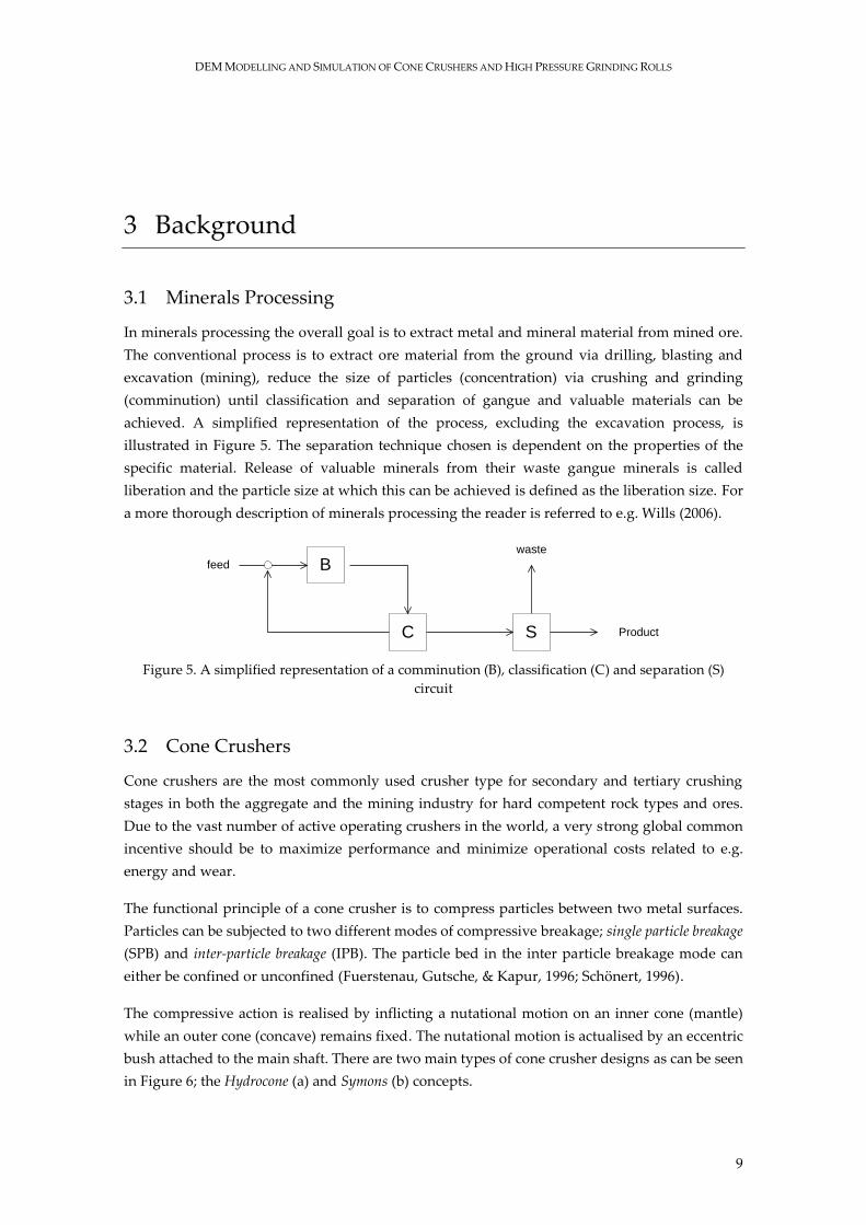
achieved. A simplified representation of the process, excluding the excavation process, is
illustrated in Figure 5. The separation technique chosen is dependent on the properties of the
specific material. Release of valuable minerals from their waste gangue minerals is called
liberation and the particle size at which this can be achieved is defined as the liberation size. For
a more thorough description of minerals processing the reader is referred to e.g. Wills (2006).
Figure 5. A simplified representation of a comminution (B), classification (C) and separation (S)
circuit
3.2 Cone Crushers
Cone crushers are the most commonly used crusher type for secondary and tertiary crushing
stages in both the aggregate and the mining industry for hard competent rock types and ores.
Due to the vast number of active operating crushers in the world, a very strong global common
incentive should be to maximize performance and minimize operational costs related to e.g.
energy and wear.
The functional principle of a cone crusher is to compress particles between two metal surfaces.
Particles can be subjected to two different modes of compressive breakage; single particle breakage
(SPB) and inter-particle breakage (IPB). The particle bed in the inter particle breakage mode can
either be confined or unconfined (Fuerstenau, Gutsche, & Kapur, 1996; Schönert, 1996).
The compressive action is realised by inflicting a nutational motion on an inner cone (mantle)
while an outer cone (concave) remains fixed. The nutational motion is actualised by an eccentric
bush attached to the main shaft. There are two main types of cone crusher designs as can be seen
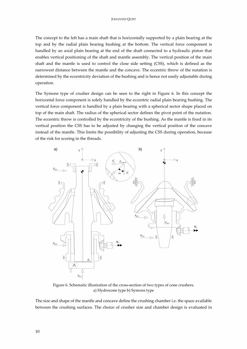
in Figure 6; the Hydrocone (a) and Symons (b) concepts.
B
C S
feed
waste
Product
JOHANNES QUIST
10
The concept to the left has a main shaft that is horizontally supported by a plain bearing at the
top and by the radial plain bearing bushing at the bottom. The vertical force component is
handled by an axial plain bearing at the end of the shaft connected to a hydraulic piston that
enables vertical positioning of the shaft and mantle assembly. The vertical position of the main
shaft and the mantle is used to control the close side setting (CSS), which is defined as the
narrowest distance between the mantle and the concave. The eccentric throw of the nutation is
determined by the eccentricity deviation of the bushing and is hence not easily adjustable during
operation.
The Symons type of crusher design can be seen to the right in Figure 6. In this concept the
horizontal force component is solely handled by the eccentric radial plain bearing bushing. The
vertical force component is handled by a plain bearing with a spherical sector shape placed on
top of the main shaft. The radius of the spherical sector defines the pivot point of the nutation.
The eccentric throw is controlled by the eccentricity of the bushing. As the mantle is fixed in its
vertical position the CSS has to be adjusted by changing the vertical position of the concave
instead of the mantle. This limits the possibility of adjusting the CSS during operation, because
of the risk for scoring in the threads.
Figure 6. Schematic illustration of the cross-section of two types of cone crushers.
a) Hydrocone type b) Symons type
The size and shape of the mantle and concave define the crushing chamber i.e. the space available
between the crushing surfaces. The choice of crusher size and chamber design is evaluated in
𝐹𝑅,1
𝐹𝑅,2
𝐹𝑅,3
𝐴𝑠
𝑀𝑣
𝛼𝐹 𝐹𝑧′
𝐹𝑥′ 𝐹𝑐𝑟𝑢𝑠 ℎ
𝐹𝑅,2
𝐹𝑅,1
𝐹𝑅,3
𝑀𝑣
z
x
z
x
a) b)
hp
DEM MODELLING AND SIMULATION OF CONE CRUSHERS AND HIGH PRESSURE GRINDING ROLLS
11
regard to the requirements on throughput capacity, ore/rock strength and the feed particle size
distribution. A comprehensive study of the performance of cone crushers has been presented by
Evertsson (2000). Hulthén developed, based on the models developed by Evertsson, a
methodology for real-time performance optimization of crushing circuits (Hulthén, 2010).
3.3 High Pressure Grinding Rolls
The high pressure grinding roll machine, often called HPGR, was originally proposed by
Schönert (Kellerwessel, 1990; Schönert, 1988) and is an adaptation of the conventional roller mill.
Many studies have been performed targeting modelling as well as circuit implementation studies,
for instance (Austin, Van Orden, & Pérez, 1980; Benzer, Aydogan, & Dündar, 2011; Daniel &
Morrell, 2004; Lim, Campbell, & Tondo, 1997; Schneider, Alves, & Austin, 2009; Schönert, 1988;
Schönert & Sander, 2002; Torres & Casali, 2009; van der Meer & Gruendken, 2010).
In order to achieve high compressive loads in interparticle breakage mode one of the rollers is
allowed to float freely and a force is applied by a hydraulic system. The hydraulic system is built
up by 2-4 pistons equipped with nitrogen gas loaded accumulators. The accumulator volume and
pressure dictates the force-displacement behaviour of the floating roller. Since a defined force-
damper action is applied the resulting working gap between the rollers will depend on the
properties of the feed material. Hence if the feed material properties change in e.g. size or
strength, a new equilibrium position will be found.
The HPGR is a complex machine system due to that the operational performance and machine
dynamics are dependent on the characteristics and compressed bed response of the feed material.
Hence it is also problematic to achieve statistical process control since obtaining low variation in
feed size distribution and ore competency is difficult in practice.
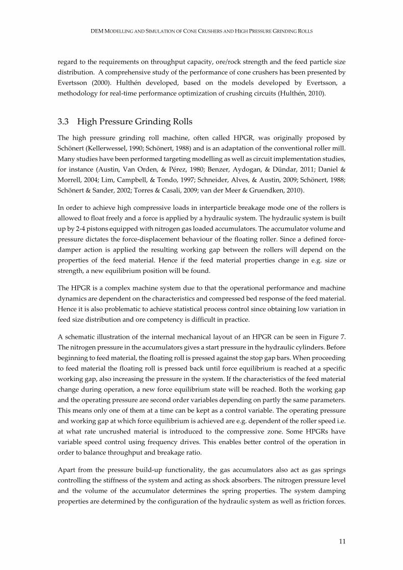
A schematic illustration of the internal mechanical layout of an HPGR can be seen in Figure 7.
The nitrogen pressure in the accumulators gives a start pressure in the hydraulic cylinders. Before
beginning to feed material, the floating roll is pressed against the stop gap bars. When proceeding
to feed material the floating roll is pressed back until force equilibrium is reached at a specific
working gap, also increasing the pressure in the system. If the characteristics of the feed material
change during operation, a new force equilibrium state will be reached. Both the working gap
and the operating pressure are second order variables depending on partly the same parameters.
This means only one of them at a time can be kept as a control variable. The operating pressure
and working gap at which force equilibrium is achieved are e.g. dependent of the roller speed i.e.
at what rate uncrushed material is introduced to the compressive zone. Some HPGRs have
variable speed control using frequency drives. This enables better control of the operation in
order to balance throughput and breakage ratio.
Apart from the pressure build-up functionality, the gas accumulators also act as gas springs
controlling the stiffness of the system and acting as shock absorbers. The nitrogen pressure level
and the volume of the accumulator determines the spring properties. The system damping
properties are determined by the configuration of the hydraulic system as well as friction forces.
JOHANNES QUIST
12
Figure 7. Schematic illustration of a high pressure grinding roll (drawing based on FLSmidth F-series
model)
3.4 Compressive Breakage
Consider a single particle captured between two plates (see Figure 1c) that are either parallel or
at an angle limited by a slip condition. A contact positioning system can be defined as the number
of contact points and their positions on either side of the particle. If a particle is resting on a
surface it will commonly be in contact at three points given that it is not either balancing on two
points, or has a surface with a flatness tolerance in parity with the plate surface (Söderberg, 1995).
Both alternative conditions can be considered unlikely for an irregular rock particle resting on a
surface. Line contact conditions are possible for cylindrical test specimens used for diametral
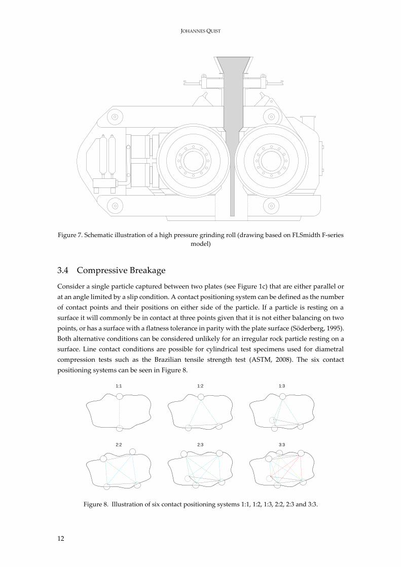
compression tests such as the Brazilian tensile strength test (ASTM, 2008). The six contact
positioning systems can be seen in Figure 8.
Figure 8. Illustration of six contact positioning systems 1:1, 1:2, 1:3, 2:2, 2:3 and 3:3.
1:1 1:2 1:3
2:32:2 3:3
DEM MODELLING AND SIMULATION OF CONE CRUSHERS AND HIGH PRESSURE GRINDING ROLLS
13
The circles in the illustration represent arbitrarily positioned contact points. Lines are drawn
between each contact point in order to visualise the relationship between the number of contact
points and the resulting stress field in the particle body.
For a particle being compressed between two surfaces at an off horizontal angle such as in a cone
crusher it is more likely that the particle may get nipped in a 2:1 or even a 1:1 contact position
system. Other positioning systems such as 2:2, 2:3 or even 3:3 are possible given certain
geometrical conditions. However for irregular particles such as rock particles those positioning
systems are less probable. The special case seen in Figure 1b with a distributed load can be
achieved by using a soft compression plate (Schönert, 1979). The position 2:1 system has been
utilized specifically in the cone crusher liner design developed by Kawasaki. The liners have a
ribbed structure on both mantle and concave in order to achieve a three point bending loading
condition.
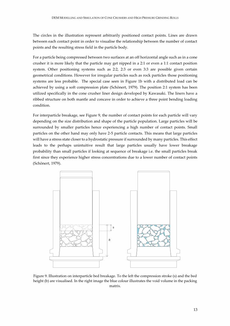
For interparticle breakage, see Figure 9, the number of contact points for each particle will vary
depending on the size distribution and shape of the particle population. Large particles will be
surrounded by smaller particles hence experiencing a high number of contact points. Small
particles on the other hand may only have 2-5 particle contacts. This means that large particles
will have a stress state closer to a hydrostatic pressure if surrounded by many particles. This effect
leads to the perhaps unintuitive result that large particles usually have lower breakage
probability than small particles if looking at sequence of breakage i.e. the small particles break
first since they experience higher stress concentrations due to a lower number of contact points
(Schönert, 1979).
Figure 9. Illustration on interparticle bed breakage. To the left the compression stroke (s) and the bed
height (b) are visualised. In the right image the blue colour illustrates the void volume in the packing
matrix.
b
s
JOHANNES QUIST
14
When studying single particle breakage under slow compression, there is a strong size-energy
relationship where more energy is needed to fracture small particles (Yashima, 1987). For impact
breakage the same relationship holds as presented by for instance, Tavares (2007). The increase
in strength with decrease in size is due to that flaws, pores and grain boundaries are distributed
in the rock body. These inhomogeneities cause stress concentrations leading to inelastic
deformations and cracks. Since the probability of finding a flaw is reduced when the particle size
decrease, the stress has to increase in order to break the particle.
Further on this leads to the conclusion that for interparticle breakage the outcome is highly
dependent on the feed size distribution and the resulting packing behaviour. For a mono sized
distribution the coordination number distribution variance will be low compared to e.g. a bi-
modal distribution where the coordination number will have a large spread.
The number of contact points in a particle packing will increase with a power law if increasing
the proportion of fine material. At each contact point there will be a stick-slip friction process
triggered by the compression. If the contact point density is high the congregated potential for
particle rearrangement also increases. Such particle rearrangement leads to heat losses due to
friction and possibly also particle surface breakage.
DEM MODELLING AND SIMULATION OF CONE CRUSHERS AND HIGH PRESSURE GRINDING ROLLS
15
4 Discrete Element Method
The discrete element method (DEM) is a numerical method for simulating discrete matter in a
series of events called time-steps. By generating particles and controlling the interaction between
them using contact models, the forces acting on all particles in the system can be calculated.
Newton’s second law of motion is then applied and the new positions of all particles are
calculated and updated for following time-step. As this process is repeated, it gives the capability
of simulating how particles move and interact in particle-boundary systems.
The method was first proposed by Cundall (1971) for the purpose of modelling blocks of rock
and later on generalized for granular materials by Cundall and Strack (1979). About 10 years later
Hart and Cundall extended the method to three dimensions (P. A. Cundall, 1988; Hart, Cundall,
& Lemos, 1988). DEM has evolved into a conventionally used 3D simulation computer aided
engineering (CAE) tool and is used by engineers and scientists in a wide range of fields. In the
pharmaceutical industry the method is e.g. used for simulating coating processes and the mixing
of powders. In the agricultural industry, DEM is used for predicting the performance of complex
sowing mechanisms. Most relevant to this work, DEM has become one of the most important
tools for simulating machines and processes within the field of minerals processing and
comminution (Weerasekara, 2013).
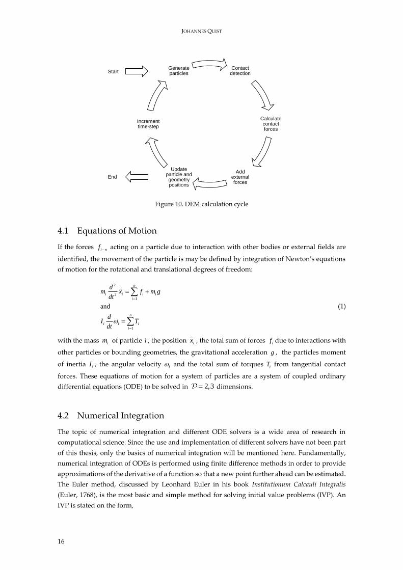
The calculation cycle of a DEM iteration can be seen in Figure 10. After initiating the simulation,
or after a previous time increment, the choice is made whether or not to generate new particles.
If particles are to be added, the type, size, orientation and position will be defined by a particle
generator function. When new particles have been created, a contact detection algorithm finds all
interaction contacts between objects in the simulation domain. The contacts may be categorised
as contacts between particles or contacts between particles and boundary objects. For all contacts
identified, the corresponding contact forces are calculated. There are several different contact
force models available, suitable for various kinds of applications, materials and conditions. For
dry granular flow the linear spring or the hertz mindlin (no slip) (HMNS) models are commonly
used. If the material has other characteristics such as moisture leading to a sticky behaviour, a
cohesion model can be used in combination with for instance HMNS. Once the forces given by
contact interactions have been calculated, any other external body forces may be added. External
forces are commonly added due to the existence of one or multiple physical fields such as
gravitational, electromagnetic or hydrodynamic fields.
In the following sections a more detailed overview of the calculation steps is presented. However,
it should be noted that the commercial software EDEM® has been used for all simulations. Hence
the descriptions on for instance equations of motion and numerical integration given below are
meant to provide coherence rather than as vital aspects of the research outcome.
JOHANNES QUIST
16
Figure 10. DEM calculation cycle
4.1 Equations of Motion
If the forces i nf acting on a particle due to interaction with other bodies or external fields are
identified, the movement of the particle is may be defined by integration of Newton’s equations
of motion for the rotational and translational degrees of freedom:
2
21
1
and
n
i i i i
i
n
i i i
i
dm x f m g
dt
dI T
dt
(1)
with the mass im of particle i , the position ix , the total sum of forces if due to interactions with
other particles or bounding geometries, the gravitational acceleration g , the particles moment
of inertia iI , the angular velocity i and the total sum of torques iT from tangential contact
forces. These equations of motion for a system of particles are a system of coupled ordinary
differential equations (ODE) to be solved in 2,3 dimensions.
4.2 Numerical Integration
The topic of numerical integration and different ODE solvers is a wide area of research in
computational science. Since the use and implementation of different solvers have not been part
of this thesis, only the basics of numerical integration will be mentioned here. Fundamentally,
numerical integration of ODEs is performed using finite difference methods in order to provide
approximations of the derivative of a function so that a new point further ahead can be estimated.
The Euler method, discussed by Leonhard Euler in his book Institutionum Calcauli Integralis
(Euler, 1768), is the most basic and simple method for solving initial value problems (IVP). An
IVP is stated on the form,
Contact detection
Calculate contact forces
Add external forces
Update particle and geometry positions
Increment time-step
Generate particlesStart
End
DEM MODELLING AND SIMULATION OF CONE CRUSHERS AND HIGH PRESSURE GRINDING ROLLS
17
, , , ,dy
y t f y t t a b y adt
(2)
Using the notation by Mattutis (2014), replacing the differential increments dy and dx by
1n ny y t y t and 1n nt t t h over the time-steps
nt and 1nt
, Equation (2) can be
rewritten to obtain the Euler method,
1,
n n
n n
y t y tyf y t t
t h
(3)
This can be rearranged to obtain the new point of interest a step forward in time 1ny t ,
1 ,n n n ny t y t h f y t t (4)
The expression in Equation (4) is termed the explicit Euler step. The slope or derivative could also
be evaluated at the next time-step 1n nt t h which leads to the implicit Euler method,
1 1 1,n n n ny t y t h f y t t (5)
In essence the Euler time-stepping method is hence based on the notion that ( , )f t y will provide
a slope of the line tangent to y at the point ( , )t y . If moving along the tangent line a small step
h t (in time), a new point 1( )ny t
will be reached. This new point will then hopefully be close
to the actual point of interest. When this is expressed using the Taylor series theorem the local
error truncation error 2( )h is added and it will accumulate as t goes from a to b . In addition
to the truncation error there will also be a rounding error when implementing the algorithm using
floating point numbers. The error will be reduced when smaller values for the step size h is
applied. Based on the principle of finite differences, several different integration methods have
been developed apart from the first order accurate explicit (forward) and implicit (backward) Euler
methods, such as for instance the Runge-Kutta methods, nth order Taylor expansions and so called
multi-step methods such as e.g. the Verlet scheme methods. The applicability of different numerical
integration schemes for DEM simulations have been investigated by for instance Kruggel-Emden
et al. (2008). Kruggel-Emden compared different integration schemes for a particle-wall contact
case and concluded that significant differences in accuracy as well as computational efficiency
could be found. In EDEM, the Symplectic Euler Method (Griffiths, 2010), also called the semi-implicit
Euler method, is the implemented approach for numerical integration. It should however be noted
that the option of choosing different integration methods have been included in the latest EDEM
2017 version.
In particle simulations the truncation and rounding errors related to the configuration and choice
of integration method are not the only source of errors. A common occurrence in DEM is that
when a too long time-step is chosen, objects with high velocities will travel a too long distance,
so that when a contact interaction has been recognised the objects are intersecting in an unnatural
way. When such high overlaps are recorded it leads to high contact forces, effectively leading to
a chain reaction explosion behaviour. This is especially critical in simulation applications with
fast moving geometry, large particle size ratios and for stiff particle systems.
JOHANNES QUIST
18
4.3 Rotation of Particles
The dynamics of the angular degrees of freedom, i.e. the rotation of bodies, can be achieved by
using the concept of Euler angles. However, the Euler angle formulation has some inherent
disadvantages leading to stability concerns. Matuttis and Chen (2014) illustrate in their DEM
textbook that for positions close to 2 and 0 the equations of motion for the Euler angles
approaches singularity conditions. In many modelling situations where Euler angles are used this
problem is avoided by appropriate selection of variables. In DEM simulations, the number of
objects are normally far higher in contrast to for instance rigid body simulations. A consequence
is that the probability of divergence of the equation of motion for some particle increases when
the number of particles increase in the simulation. A remedy to the singularity problem of Euler
angles is to use the method called quaternions. The quaternion formulation is based on using
complex number theory and provides a very stable representation of the equations of motion for
the angular degrees of freedom (Matuttis, 2014). For the conventional full mathematical
formulation of the Euler angle and quaternion concepts, see for instance Matuttis (2014) or
Wittenburg (2008).
4.4 Contact Detection
Before being able to calculate the resulting force from a particle-particle or particle-wall
interaction, the existence of all contacts needs to be identified. The algorithms for finding contacts
are called broad phase collision detection. The most simple contact detection algorithm is
sometimes called the brute force method. If assuming a system of N particles, then the brute
force method constitutes checking each particle against all other particles leading to order 2( )O N
operations (Weller, 2013). The method is computationally inefficient hence other more
sophisticated approaches are normally applied in simulations where particles and other objects
interact.
The neighbouring cell method, which is used in EDEM, divides the simulation domain into a grid
of cells with a size usually specified by a ratio to the particle size. A list is kept of particles
contained in each cell and for each particle, only the particles in the same and neighbouring cells
needs to be checked for contact. A consequence of this strategy is the trade-off between having a
large number of cells (small cell size) versus having too many particles to check in each operation
(large cell size).
Other examples of contact detection algorithms used in DEM are the nearest neighbour method
(Vu-Quoc, Zhang, & Walton, 2000; Zhao, Nezami, Hashash, & Ghaboussi, 2006) where a
bounding volume is used to create a list of neighbouring particles, and the sweep and prune
method (Perkins & Williams, 2001) where bounding volumes and edge projections to each axis
direction are used to create a list that can be sorted in order to identify which bounding volumes
that are candidates for overlap. These different methods have advantages and disadvantages
depending on the simulation application. The nearest neighbour method is for instance suitable
for quasi-static simulations where particles do not re-arrange or move large distances. In cases
DEM MODELLING AND SIMULATION OF CONE CRUSHERS AND HIGH PRESSURE GRINDING ROLLS
19
with large particle size differences, sweep and prune as well as other hierarchy methods are
suitable.
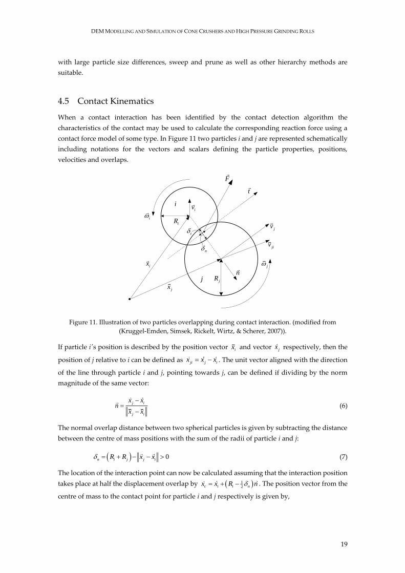
4.5 Contact Kinematics
When a contact interaction has been identified by the contact detection algorithm the
characteristics of the contact may be used to calculate the corresponding reaction force using a
contact force model of some type. In Figure 11 two particles i and j are represented schematically
including notations for the vectors and scalars defining the particle properties, positions,
velocities and overlaps.
Figure 11. Illustration of two particles overlapping during contact interaction. (modified from
(Kruggel-Emden, Simsek, Rickelt, Wirtz, & Scherer, 2007)).
If particle i's position is described by the position vector ix and vector jx respectively, then the
position of j relative to i can be defined as ji j ix x x . The unit vector aligned with the direction
of the line through particle i and j, pointing towards j, can be defined if dividing by the norm
magnitude of the same vector:
j i
j i
x xn
x x
(6)
The normal overlap distance between two spherical particles is given by subtracting the distance
between the centre of mass positions with the sum of the radii of particle i and j:
0n i j j iR R x x (7)
The location of the interaction point can now be calculated assuming that the interaction position
takes place at half the displacement overlap by 1
2c i i nx x R n . The position vector from the
centre of mass to the contact point for particle i and j respectively is given by,
i
j
j
i
ix
jxjR
iR
iv
jv
jiv
t
n
F
n
t
JOHANNES QUIST
20
1, 2
1, 2
i c i n
j c j n
r R n
r R n
(8)
The velocity vector at the contact point can now be written as , ,i c i i i cv v r for particle i and as
, ,j c j j j cv v r for particle j. The relative velocity vector of the interaction contact point is given
by rel, , ,c j c i cv v v . The normal and tangential unit vectors can further on be used to achieve a
separation of the normal and tangential component so that rel, rel, rel,c c cv v n n v t t . We can
now write the tangential unit vector as,
rel, rel,
rel, rel,
c c
c c
v v n nt
v v n n
(9)
The tangential overlap distance is then given by,
rel,t cv t dt (10)
where dt is the time-step.
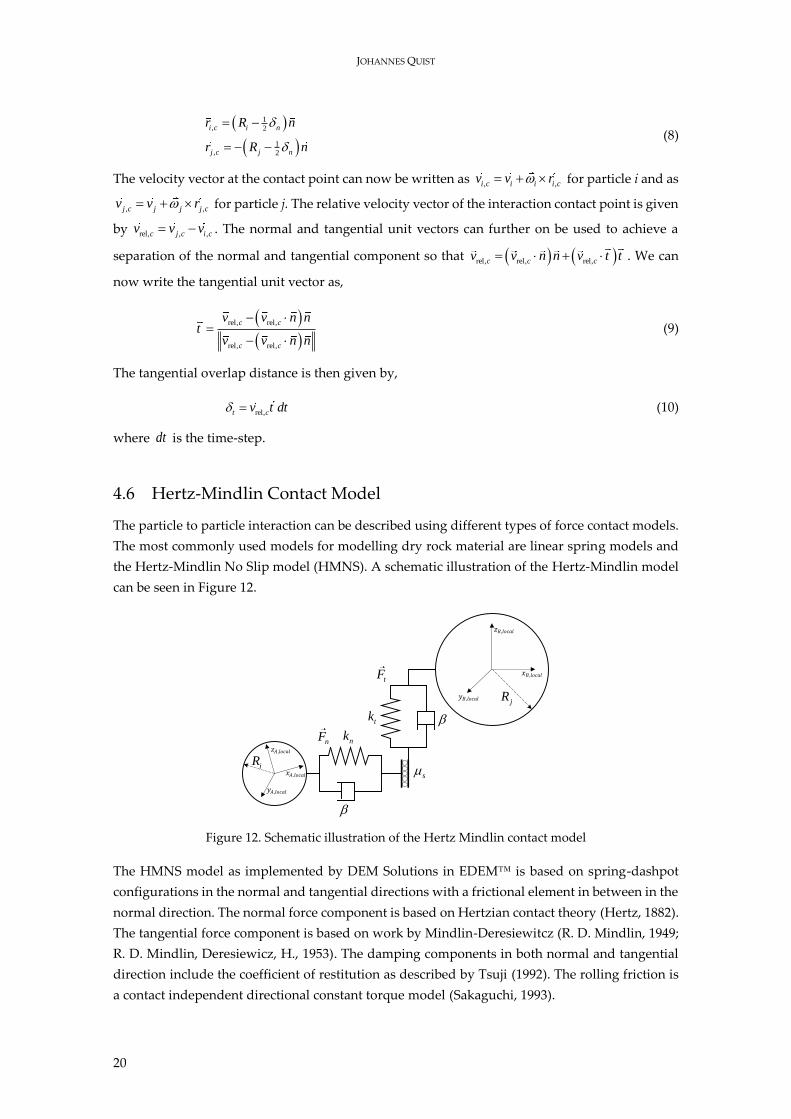
4.6 Hertz-Mindlin Contact Model
The particle to particle interaction can be described using different types of force contact models.
The most commonly used models for modelling dry rock material are linear spring models and
the Hertz-Mindlin No Slip model (HMNS). A schematic illustration of the Hertz-Mindlin model
can be seen in Figure 12.
Figure 12. Schematic illustration of the Hertz Mindlin contact model
The HMNS model as implemented by DEM Solutions in EDEM™ is based on spring-dashpot
configurations in the normal and tangential directions with a frictional element in between in the
normal direction. The normal force component is based on Hertzian contact theory (Hertz, 1882).
The tangential force component is based on work by Mindlin-Deresiewitcz (R. D. Mindlin, 1949;
R. D. Mindlin, Deresiewicz, H., 1953). The damping components in both normal and tangential
direction include the coefficient of restitution as described by Tsuji (1992). The rolling friction is
a contact independent directional constant torque model (Sakaguchi, 1993).
𝑥𝐵 ,𝑙𝑜𝑐𝑎𝑙
𝑦𝐵 ,𝑙𝑜𝑐𝑎𝑙
𝑧𝐵,𝑙𝑜𝑐𝑎𝑙
𝑦𝐴,𝑙𝑜𝑐𝑎𝑙
𝑥𝐴,𝑙𝑜𝑐𝑎𝑙
𝑧𝐴,𝑙𝑜𝑐𝑎𝑙
tF
nF nk
tk
siR
jR
DEM MODELLING AND SIMULATION OF CONE CRUSHERS AND HIGH PRESSURE GRINDING ROLLS
21
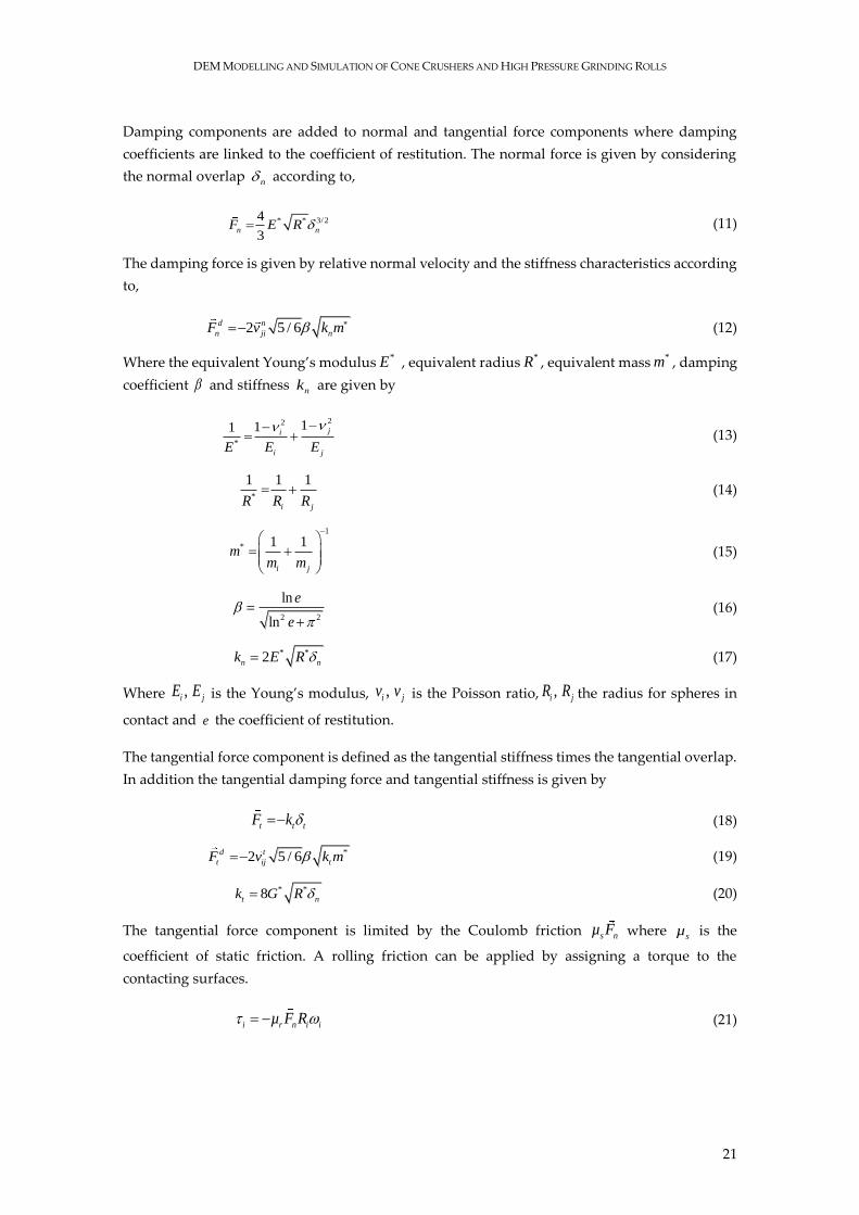
Damping components are added to normal and tangential force components where damping
coefficients are linked to the coefficient of restitution. The normal force is given by considering
the normal overlap n according to,
* * 3/24 3
n nF E R (11)
The damping force is given by relative normal velocity and the stiffness characteristics according
to,
2 5 / 6n
j
d
n i nF v k m (12)
Where the equivalent Young’s modulus *E , equivalent radius *R , equivalent mass *m , damping
coefficient and stiffness nk are given by
22
*
111
ji
i jE EE
(13)
*
1 1 1
i jR RR (14)
1
* 1 1
i j
mm m
(15)
2 2
ln
ln
e
e
(16)
* *2n nk E R (17)
Where ,i jE E is the Young’s modulus, ,i jv v is the Poisson ratio, ,i jR R the radius for spheres in
contact and e the coefficient of restitution.
The tangential force component is defined as the tangential stiffness times the tangential overlap.
In addition the tangential damping force and tangential stiffness is given by
tt tF k (18)
* 2 5 / 6t
i
d
t tjF v k m (19)
* *8t nk G R (20)
The tangential force component is limited by the Coulomb friction s nµ F where sµ is the
coefficient of static friction. A rolling friction can be applied by assigning a torque to the
contacting surfaces.
i r n i iµ F R (21)
JOHANNES QUIST
22
With i being the unit angular velocity vector of the object at the contact point,
rµ the
coefficient of rolling friction and iR the distance between the centre of mass and the contact
point.
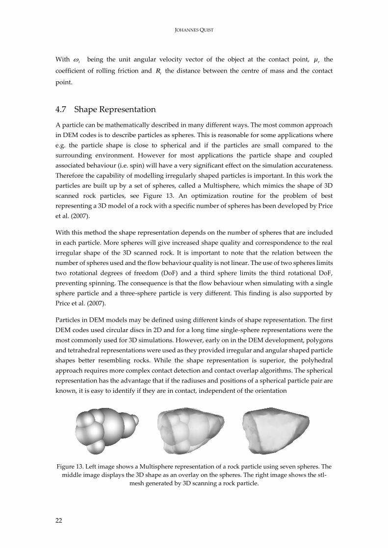
4.7 Shape Representation
A particle can be mathematically described in many different ways. The most common approach
in DEM codes is to describe particles as spheres. This is reasonable for some applications where
e.g. the particle shape is close to spherical and if the particles are small compared to the
surrounding environment. However for most applications the particle shape and coupled
associated behaviour (i.e. spin) will have a very significant effect on the simulation accurateness.
Therefore the capability of modelling irregularly shaped particles is important. In this work the
particles are built up by a set of spheres, called a Multisphere, which mimics the shape of 3D
scanned rock particles, see Figure 13. An optimization routine for the problem of best
representing a 3D model of a rock with a specific number of spheres has been developed by Price
et al. (2007).
With this method the shape representation depends on the number of spheres that are included
in each particle. More spheres will give increased shape quality and correspondence to the real
irregular shape of the 3D scanned rock. It is important to note that the relation between the
number of spheres used and the flow behaviour quality is not linear. The use of two spheres limits
two rotational degrees of freedom (DoF) and a third sphere limits the third rotational DoF,
preventing spinning. The consequence is that the flow behaviour when simulating with a single
sphere particle and a three-sphere particle is very different. This finding is also supported by
Price et al. (2007).
Particles in DEM models may be defined using different kinds of shape representation. The first
DEM codes used circular discs in 2D and for a long time single-sphere representations were the
most commonly used for 3D simulations. However, early on in the DEM development, polygons
and tetrahedral representations were used as they provided irregular and angular shaped particle
shapes better resembling rocks. While the shape representation is superior, the polyhedral
approach requires more complex contact detection and contact overlap algorithms. The spherical
representation has the advantage that if the radiuses and positions of a spherical particle pair are
known, it is easy to identify if they are in contact, independent of the orientation
Figure 13. Left image shows a Multisphere representation of a rock particle using seven spheres. The
middle image displays the 3D shape as an overlay on the spheres. The right image shows the stl-
mesh generated by 3D scanning a rock particle.
DEM MODELLING AND SIMULATION OF CONE CRUSHERS AND HIGH PRESSURE GRINDING ROLLS
23
4.8 Breakage Models
In systems where the loading condition does not significantly influence the particle integrity, no
specific breakage model is needed. In these cases Hertzian or linear spring contact models are
commonly used. However, when using DEM to understand the mechanisms in comminution
devices, where the destruction of solids is the objective, a breakage modelling approach is needed.
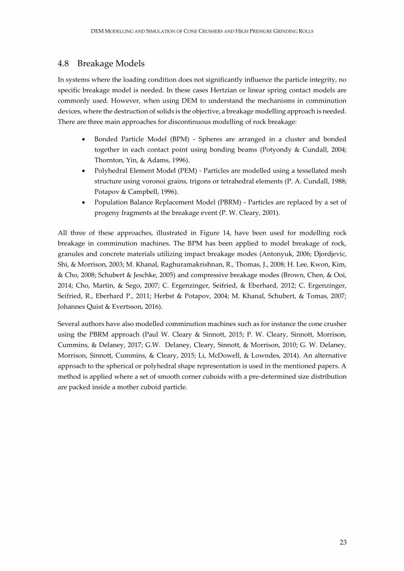
There are three main approaches for discontinuous modelling of rock breakage:
Bonded Particle Model (BPM) - Spheres are arranged in a cluster and bonded
together in each contact point using bonding beams (Potyondy & Cundall, 2004;
Thornton, Yin, & Adams, 1996).
Polyhedral Element Model (PEM) - Particles are modelled using a tessellated mesh
structure using voronoi grains, trigons or tetrahedral elements (P. A. Cundall, 1988;
Potapov & Campbell, 1996).
Population Balance Replacement Model (PBRM) - Particles are replaced by a set of
progeny fragments at the breakage event (P. W. Cleary, 2001).
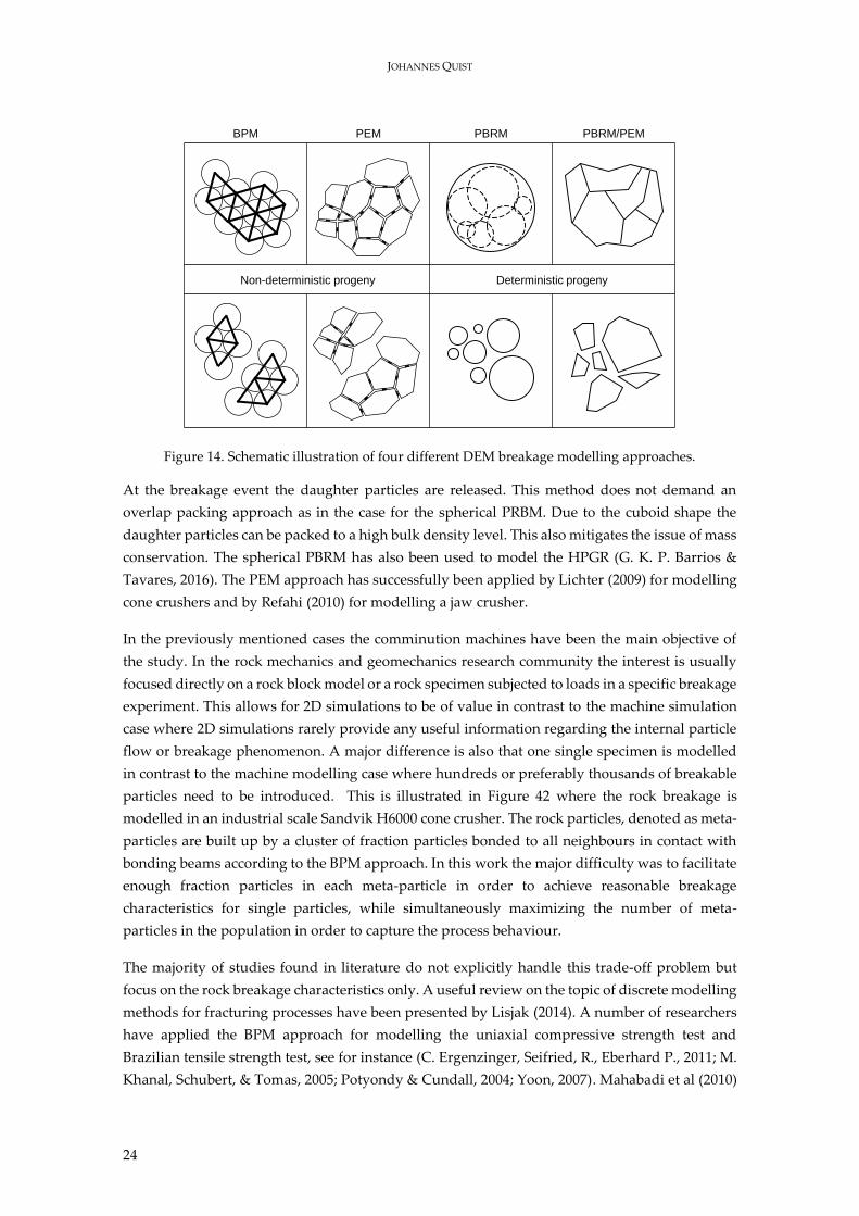
All three of these approaches, illustrated in Figure 14, have been used for modelling rock
breakage in comminution machines. The BPM has been applied to model breakage of rock,
granules and concrete materials utilizing impact breakage modes (Antonyuk, 2006; Djordjevic,
Shi, & Morrison, 2003; M. Khanal, Raghuramakrishnan, R., Thomas, J., 2008; H. Lee, Kwon, Kim,
& Cho, 2008; Schubert & Jeschke, 2005) and compressive breakage modes (Brown, Chen, & Ooi,
2014; Cho, Martin, & Sego, 2007; C. Ergenzinger, Seifried, & Eberhard, 2012; C. Ergenzinger,
Seifried, R., Eberhard P., 2011; Herbst & Potapov, 2004; M. Khanal, Schubert, & Tomas, 2007;
Johannes Quist & Evertsson, 2016).
Several authors have also modelled comminution machines such as for instance the cone crusher
using the PBRM approach (Paul W. Cleary & Sinnott, 2015; P. W. Cleary, Sinnott, Morrison,
Cummins, & Delaney, 2017; G.W. Delaney, Cleary, Sinnott, & Morrison, 2010; G. W. Delaney,
Morrison, Sinnott, Cummins, & Cleary, 2015; Li, McDowell, & Lowndes, 2014). An alternative
approach to the spherical or polyhedral shape representation is used in the mentioned papers. A
method is applied where a set of smooth corner cuboids with a pre-determined size distribution
are packed inside a mother cuboid particle.
JOHANNES QUIST
24
Figure 14. Schematic illustration of four different DEM breakage modelling approaches.
At the breakage event the daughter particles are released. This method does not demand an
overlap packing approach as in the case for the spherical PRBM. Due to the cuboid shape the
daughter particles can be packed to a high bulk density level. This also mitigates the issue of mass
conservation. The spherical PBRM has also been used to model the HPGR (G. K. P. Barrios &
Tavares, 2016). The PEM approach has successfully been applied by Lichter (2009) for modelling
cone crushers and by Refahi (2010) for modelling a jaw crusher.
In the previously mentioned cases the comminution machines have been the main objective of
the study. In the rock mechanics and geomechanics research community the interest is usually
focused directly on a rock block model or a rock specimen subjected to loads in a specific breakage
experiment. This allows for 2D simulations to be of value in contrast to the machine simulation
case where 2D simulations rarely provide any useful information regarding the internal particle
flow or breakage phenomenon. A major difference is also that one single specimen is modelled
in contrast to the machine modelling case where hundreds or preferably thousands of breakable
particles need to be introduced. This is illustrated in Figure 42 where the rock breakage is
modelled in an industrial scale Sandvik H6000 cone crusher. The rock particles, denoted as meta-
particles are built up by a cluster of fraction particles bonded to all neighbours in contact with
bonding beams according to the BPM approach. In this work the major difficulty was to facilitate
enough fraction particles in each meta-particle in order to achieve reasonable breakage
characteristics for single particles, while simultaneously maximizing the number of meta-
particles in the population in order to capture the process behaviour.
The majority of studies found in literature do not explicitly handle this trade-off problem but
focus on the rock breakage characteristics only. A useful review on the topic of discrete modelling
methods for fracturing processes have been presented by Lisjak (2014). A number of researchers
have applied the BPM approach for modelling the uniaxial compressive strength test and
Brazilian tensile strength test, see for instance (C. Ergenzinger, Seifried, R., Eberhard P., 2011; M.
Khanal, Schubert, & Tomas, 2005; Potyondy & Cundall, 2004; Yoon, 2007). Mahabadi et al (2010)
BPM PEM PBRM PBRM/PEM
Deterministic progeny Non-deterministic progeny
DEM MODELLING AND SIMULATION OF CONE CRUSHERS AND HIGH PRESSURE GRINDING ROLLS
25
modelled the diametrical compression of rock discs in the split Hopkinson bar by applying a
hybrid finite-discrete element method in 2D formulated by Munjiza (2004). In the FEM/DEM
method each discrete element is discretised into a mesh of finite elements. This means that the
discontinuum behaviour is modelled by discrete elements and the continuum behaviour through
finite elements. The transition between the continuum and discontinuum is handled through
defining a fragmentation process, leading to the ability of modelling breakage.
Kazerani (2013) used a discontinuum based model implemented in the UDEC (Itasca Consulting
Group, 2008) software package for modelling both compressive and tensile failure of sedimentary
rock. The 2D model is based on a finite difference discrete element approach where the micro-
structure is modelled as an assembly of distinct mesh elements whose boundary behaviour is
controlled by contact models. The authors applied a central composite design experimental plan
to calibrate and analyse the statistical influence of a set of micro parameters controlling the
breakage behaviour. The resulting fracture patterns resemble the experimental results in both the
uniaxial strength test as well as the Brazilian tensile strength test. Similar 2D studies have also
been conducted by Tatone et al (2015) and Ghazvinian et al (2014) using a Delaunay algorithm to
generate a Voronoi mesh which incorporates the possibility of modelling complex crystalline
grain structures.
Recently, Behraftar et al (2017) presented a methodology for the evaluation of micro parameters
of a breakage model based on a method named discrete sphero-polyhedral element method
(DSEM). In three dimensions each element is modelled as a polyhedral where the corners have
been rounded. Due to the smoothness of all geometrical features the handling of contacts between
elements becomes simple and efficient. The simulation results showed a good agreement to the
Cracked Chevron Notched Brazilian Discs (CCNBD) breakage experiment.
The smooth particle hydrodynamics (SPH) method has also been applied to fracture modelling
by for instance Das and Cleary (2010) and Ma (2011). Since SPH is a mesh-free method it has an
advantage over mesh-based models when it comes to for instance, high deformations and self-
collision. The results presented by Das (2010) using the 2D SPH fracture model for different
geometrical shapes showed a good qualitative behaviour when comparing fracture patterns.
Nishioka (1997) states in his review article that for continuum modelling approaches for fracture
mechanics, there are three primary methods; the finite difference method (FDM), the finite-
element method (FEM), and the boundary-element method (BEM). These continuum based
models will not be further elaborated on or discussed in the paper specifically. However, the
general calibration approach presented below would principally be applicable also in these cases.
4.9 Bonded Particle Model
The bonded particle model (BPM) was formulated by Potyondy and Cundall (2004) for the
purpose of simulating rock breakage. The approach has been applied and further developed by
Cho (2007). The concept is based on bonding or gluing a packed distribution of spheres together
forming a breakable body. The particles bonded together will hereafter be called fraction particles
and the cluster created is defined as a meta-particle. The fraction particles can either be of mono
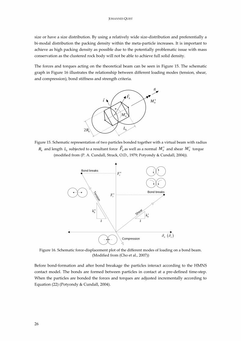
JOHANNES QUIST
26
size or have a size distribution. By using a relatively wide size-distribution and preferentially a
bi-modal distribution the packing density within the meta-particle increases. It is important to
achieve as high packing density as possible due to the potentially problematic issue with mass
conservation as the clustered rock body will not be able to achieve full solid density.
The forces and torques acting on the theoretical beam can be seen in Figure 15. The schematic
graph in Figure 16 illustrates the relationship between different loading modes (tension, shear,
and compression), bond stiffness and strength criteria.
Figure 15. Schematic representation of two particles bonded together with a virtual beam with radius
bR and length bL subjected to a resultant force bF as well as a normal
n
bM and shear
s
bM torque
(modified from (P. A. Cundall, Strack, O.D., 1979; Potyondy & Cundall, 2004)).
Figure 16. Schematic force-displacement plot of the different modes of loading on a bond beam.
(Modified from (Cho et al., 2007))
Before bond-formation and after bond breakage the particles interact according to the HMNS
contact model. The bonds are formed between particles in contact at a pre-defined time-step.
When the particles are bonded the forces and torques are adjusted incrementally according to
Equation (22) (Potyondy & Cundall, 2004).
2 bR
t
n
n
bMbF
s
bM
bL
Bond breaks
Bond breaks
Compression
Tensio
n
Shear
1 1
n
cF
s
cF
n
bks
bk
n s
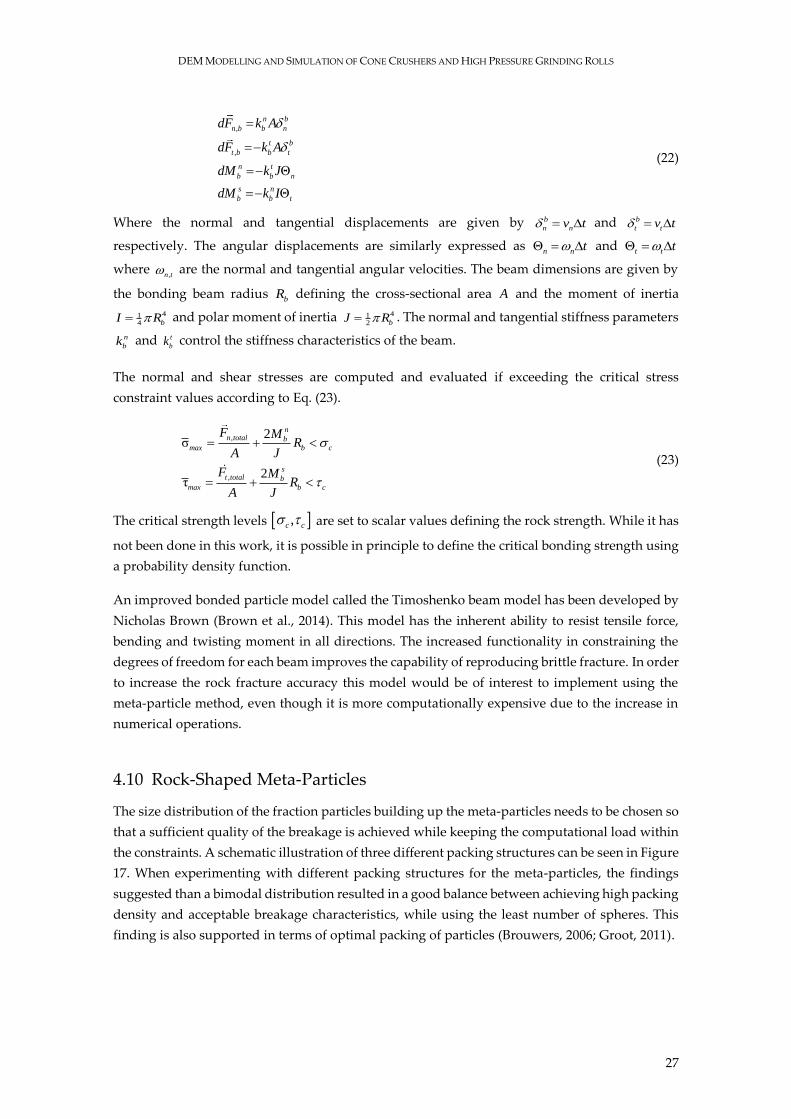
DEM MODELLING AND SIMULATION OF CONE CRUSHERS AND HIGH PRESSURE GRINDING ROLLS
27
,
,
Θ
Θ
n b
n b b n
t b
t b b t
n t
b b n
s n
b b t
dF k A
dF k A
dM k J
k IdM
(22)
Where the normal and tangential displacements are given by n
b
n v t and b
t tv t
respectively. The angular displacements are similarly expressed as Θn n t and Θt t t
where ,n t are the normal and tangential angular velocities. The beam dimensions are given by
the bonding beam radius bR defining the cross-sectional area A and the moment of inertia
414 bI R and polar moment of inertia 41
2 bJ R . The normal and tangential stiffness parameters
n
bk and t
bk control the stiffness characteristics of the beam.
The normal and shear stresses are computed and evaluated if exceeding the critical stress
constraint values according to Eq. (23).
,
,
2σ
2τ
nn total b
max b c
st total b
max b c
F MR
A J
F MR
A J
(23)
The critical strength levels ,c c are set to scalar values defining the rock strength. While it has
not been done in this work, it is possible in principle to define the critical bonding strength using
a probability density function.
An improved bonded particle model called the Timoshenko beam model has been developed by
Nicholas Brown (Brown et al., 2014). This model has the inherent ability to resist tensile force,
bending and twisting moment in all directions. The increased functionality in constraining the
degrees of freedom for each beam improves the capability of reproducing brittle fracture. In order
to increase the rock fracture accuracy this model would be of interest to implement using the
meta-particle method, even though it is more computationally expensive due to the increase in
numerical operations.
4.10 Rock-Shaped Meta-Particles
The size distribution of the fraction particles building up the meta-particles needs to be chosen so
that a sufficient quality of the breakage is achieved while keeping the computational load within
the constraints. A schematic illustration of three different packing structures can be seen in Figure
17. When experimenting with different packing structures for the meta-particles, the findings
suggested than a bimodal distribution resulted in a good balance between achieving high packing
density and acceptable breakage characteristics, while using the least number of spheres. This
finding is also supported in terms of optimal packing of particles (Brouwers, 2006; Groot, 2011).
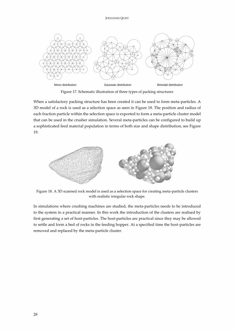
JOHANNES QUIST
28
Figure 17. Schematic illustration of three types of packing structures
When a satisfactory packing structure has been created it can be used to form meta-particles. A
3D model of a rock is used as a selection space as seen in Figure 18. The position and radius of
each fraction particle within the selection space is exported to form a meta-particle cluster model
that can be used in the crusher simulation. Several meta-particles can be configured to build up
a sophisticated feed material population in terms of both size and shape distribution, see Figure
19.
Figure 18. A 3D scanned rock model is used as a selection space for creating meta-particle clusters
with realistic irregular rock shape.
In simulations where crushing machines are studied, the meta-particles needs to be introduced
to the system in a practical manner. In this work the introduction of the clusters are realised by
first generating a set of host-particles. The host-particles are practical since they may be allowed
to settle and form a bed of rocks in the feeding hopper. At a specified time the host-particles are
removed and replaced by the meta-particle cluster.
Mono distribution
-
-
--
-
--
- -
-
-
-
--
-
-
-
---
-
-
-
- -
-
---
-
--
-
Gaussian distribution
-
-
--
-
-
-
--
--
- -
-
-
-
-
-
- -
--
-
-
Bimodal distribution
-
-
--
-
-
- -
- -
-
--
-
-
-
-
-
-
--
--
-- -
-
-
---
--
--
-
-
--
-
- -
-
-
-
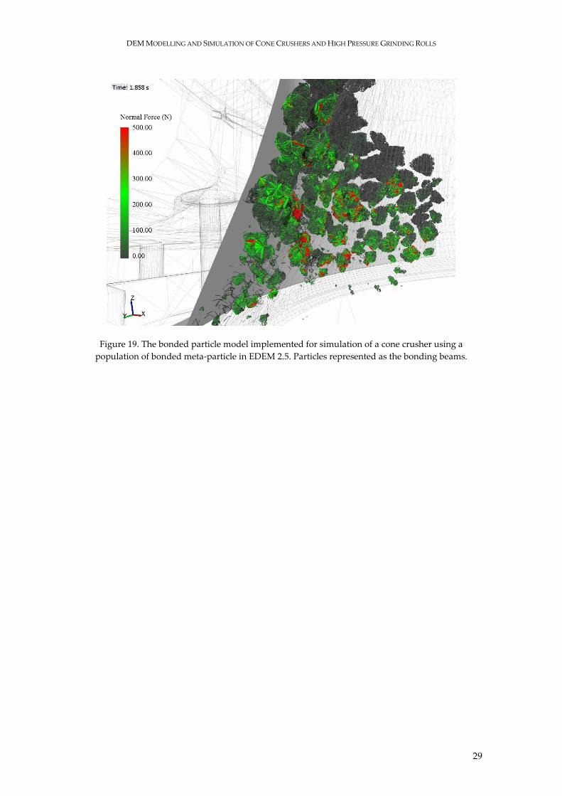
DEM MODELLING AND SIMULATION OF CONE CRUSHERS AND HIGH PRESSURE GRINDING ROLLS
29
Figure 19. The bonded particle model implemented for simulation of a cone crusher using a
population of bonded meta-particle in EDEM 2.5. Particles represented as the bonding beams.

JOHANNES QUIST
30
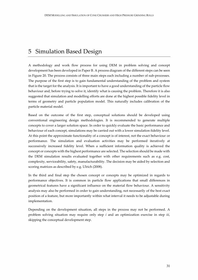
DEM MODELLING AND SIMULATION OF CONE CRUSHERS AND HIGH PRESSURE GRINDING ROLLS
31
5 Simulation Based Design
A methodology and work flow process for using DEM in problem solving and concept
development has been developed in Paper B. A process diagram of the different steps can be seen
in Figure 20. The process consists of three main steps each including a number of sub-processes.
The purpose of the first step is to gain fundamental understanding of the problem and system
that is the target for the analysis. It is important to have a good understanding of the particle flow
behaviour and, before trying to solve it, identify what is causing the problem. Therefore it is also
suggested that simulation and modelling efforts are done at the highest possible fidelity level in
terms of geometry and particle population model. This naturally includes calibration of the
particle material model.
Based on the outcome of the first step, conceptual solutions should be developed using
conventional engineering design methodologies. It is recommended to generate multiple
concepts to cover a larger solution space. In order to quickly evaluate the basic performance and
behaviour of each concept, simulations may be carried out with a lower simulation fidelity level.
At this point the approximate functionality of a concept is of interest, not the exact behaviour or
performance. The simulation and evaluation activities may be performed iteratively at
successively increased fidelity level. When a sufficient information quality is achieved the
concept or concepts with the highest performance are selected. The selection should be made with
the DEM simulation results evaluated together with other requirements such as e.g. cost,
complexity, serviceability, safety, manufacturability. The decision may be aided by selection and
scoring matrices as described by e.g. Ulrich (2008).
In the third and final step the chosen concept or concepts may be optimized in regards to
performance objectives. It is common in particle flow applications that small differences in
geometrical features have a significant influence on the material flow behaviour. A sensitivity
analysis may also be performed in order to gain understanding, not necessarily of the best exact
position of a feature, but more importantly within what interval it needs to be adjustable during
implementation.
Depending on the development situation, all steps in the process may not be performed. A
problem solving situation may require only step i and an optimization exercise in step iii,
skipping the conceptual development step.
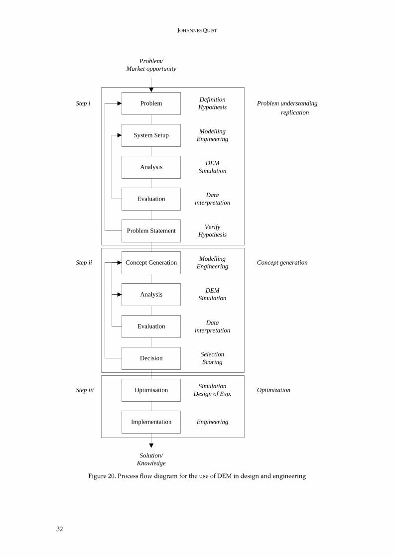
JOHANNES QUIST
32
Figure 20. Process flow diagram for the use of DEM in design and engineering
Problem
System Setup
Analysis
Evaluation
Problem Statement
Concept Generation
Analysis
Evaluation
Decision
Optimisation
Implementation
Definition
Hypothesis
Modelling
Engineering
DEM
Simulation
Data
interpretation
Verify
Hypothesis
Modelling
Engineering
DEM
Simulation
Data
interpretation
Selection
Scoring
Simulation
Design of Exp.
Engineering
Step i
Step ii
Step iii
Problem/
Market opportunity
Solution/
Knowledge
Problem understanding
replication
Concept generation
Optimization
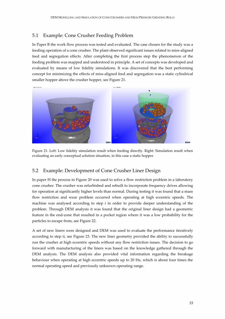
DEM MODELLING AND SIMULATION OF CONE CRUSHERS AND HIGH PRESSURE GRINDING ROLLS
33
5.1 Example: Cone Crusher Feeding Problem
In Paper B the work flow process was tested and evaluated. The case chosen for the study was a
feeding operation of a cone crusher. The plant observed significant issues related to miss-aligned
feed and segregation effects. After completing the first process step the phenomenon of the
feeding problem was mapped and understood in principle. A set of concepts was developed and
evaluated by means of low fidelity simulations. It was discovered that the best performing
concept for minimizing the effects of miss-aligned feed and segregation was a static cylindrical
smaller hopper above the crusher hopper, see Figure 21.
Figure 21. Left: Low fidelity simulation result when feeding directly. Right: Simulation result when
evaluating an early conceptual solution situation, in this case a static hopper.
5.2 Example: Development of Cone Crusher Liner Design
In paper H the process in Figure 20 was used to solve a flow restriction problem in a laboratory
cone crusher. The crusher was refurbished and rebuilt to incorporate frequency drives allowing
for operation at significantly higher levels than normal. During testing it was found that a mass
flow restriction and wear problem occurred when operating at high eccentric speeds. The
machine was analysed according to step i in order to provide deeper understanding of the
problem. Through DEM analysis it was found that the original liner design had a geometric
feature in the end-zone that resulted in a pocket region where it was a low probability for the
particles to escape from, see Figure 22.
A set of new liners were designed and DEM was used to evaluate the performance iteratively
according to step ii, see Figure 23. The new liner geometry provided the ability to successfully
run the crusher at high eccentric speeds without any flow restriction issues. The decision to go
forward with manufacturing of the liners was based on the knowledge gathered through the
DEM analysis. The DEM analysis also provided vital information regarding the breakage
behaviour when operating at high eccentric speeds up to 20 Hz, which is about four times the
normal operating speed and previously unknown operating range.
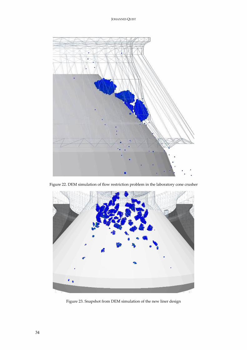
JOHANNES QUIST
34
Figure 22. DEM simulation of flow restriction problem in the laboratory cone crusher
Figure 23. Snapshot from DEM simulation of the new liner design
DEM MODELLING AND SIMULATION OF CONE CRUSHERS AND HIGH PRESSURE GRINDING ROLLS
35
6 Verification and Validation
Currently, the assessment of whether comminution and crushing equipment under development
satisfies stated functional requirements is commonly expensive due to the need for numerous
resource intensive physical experiments. Computer modelling and simulation-based methods for
virtual comminution analysis and design evaluation currently have an increasing impact on the
time and cost effectiveness of the development process (Forrester, Keane, & Sóbester, 2008). To
accomplish the benefits of virtual testing, simulation-based predictions require verification and
validation. Evidently, the virtual testing must also provide the sought insight and knowledge at
a lower cost and time compared to physical tests.
The ASME (American Society of Mechanical Engineers) guide for Verification and Validation in
Computational Solid Mechanics (2006), provides the following definitions,
Verification: The process of determining that a computational model accurately
represents the underlying mathematical model and its solution.
Validation: The process of determining the degree to which a model is an accurate
representation of the real world from the perspective of the intended uses of the model.
The desired outcome of the verification and validation (V&V) process is to validate the model for
its intended use (ASME, 2006; Sargent, 2013). This is an important distinction to make in the
context of design engineering. The model builder needs to define a set of predetermined
requirements setting the constraints for the accuracy and predictive capability. The accuracy
constraint may in some cases be balanced against computational load in a trade-off exercise.
Meaning that some modelling accuracy is intentionally sacrificed in order to run fast simulations.
This model fidelity reduction has to be accounted for in the decision making process. It is hence
also advisable to exercise some caution regarding which stakeholders are to be included, and how
they are informed, before entering the decision making process.
An example of this strategy is demonstrated in Paper B, previously described in §5 where a lower
fidelity DEM particle material model is used for preliminary virtual experiments of several
different conceptual design solutions for a cone crusher feeding problem. In many cases when
dealing with particle flow problem solving it is difficult to, based on engineering heuristics and
experience, make a decent prediction regarding the particle trajectories and segregation
behaviour. This is especially the case when a stream of particles interacts with equipment put in
place with the intended function to guide or mix the material. For initial conceptual evaluations
it is advantageous to perform quick simulations with computational times below 2-15 minutes.
This allows for iterative adjustment of geometrical features (shape and position) until the
conceptual solution reaches a sufficient performance to be further analysed.
JOHANNES QUIST
36
As a part of the previously mentioned study in Paper B, the design stage process is proposed for
particle flow problem solving using DEM, see Figure 20. In this process the first step is to perform
a high fidelity simulation with the purpose of understanding the current problem. For this step
it is not advisable to reduce the model fidelity in order to save computational time. This analysis
stage is important in order to reproduce the issues reported and measured in operation. If the
operational problems (e.g. miss-aligned feeding, segregation effects or blockages) cannot be
reproduced, the modelling needs to be revisited, improved and iterated. This kind of direct visual
semi-validation leads to an interesting point regarding alternative validation methods for cases
where it is expensive or not possible to perform direct measurements on complex and disruptive
particle flow conditions.
Other methods for validation than to mathematically compare datasets are mentioned in the
model validation research field. A number of different validation techniques have been listed by
Sargent (2013). One of the approaches mentioned is defined as ‘face validity’ and is explained as
validation based on the engineering individuals knowledge and experience about the system. In
the case of DEM modelling and simulation, experienced engineers and researchers may comment
that a simulation appears to be realistic. Such a comment obviously does not automatically
validate a simulation model. However, in cases where direct measurement is difficult and
expensive, it might still be of value to the model developer.
According to the terminology and framework proposed by Schlesinger et al (1979) validation may
also be done in regards to the conceptual model of a system. There are several examples in this
work where the simulation results have been evaluated in regards to an expected behaviour
based on an already established conceptual model:
The observed edge effect of the pressure distribution from the HPGR simulations in
Paper D. Described by e.g. (Daniel & Morrell, 2004; Schönert & Sander, 2002; Torres &
Casali, 2009) and measured by (Lubjuhn, 1994).
The observed choke level in the cone crusher and its dependence on the position of the
minimum cross sectional area in the crusher chamber (Paper A, C, F).
The observed phenomenon of inter particle breakage above the choke level and single
particle breakage happening below the choke level in (Paper A, F). As proposed by
Evertsson (C.M. Evertsson, 2000).
The relationship between the eccentric speed and the number of breakage zones (Paper
A). As proposed by Evertsson (C.M. Evertsson, 2000).
Due to the difficulty of measurement directly in an industrial operation, the process validation
needs to be decomposed into manageable sub-models. This decomposition into a hierarchical
approach to validation is discussed in the ASME standard (ASME, 2006). A bottom-up approach,
exemplified by a vehicle model application, is suggested where the lowest level of models, called
component models, are validated using experiments. The component level is followed by
subassembly models, assembly models, system models, finally achieving a validated model
applicable to the top level reality of interest.
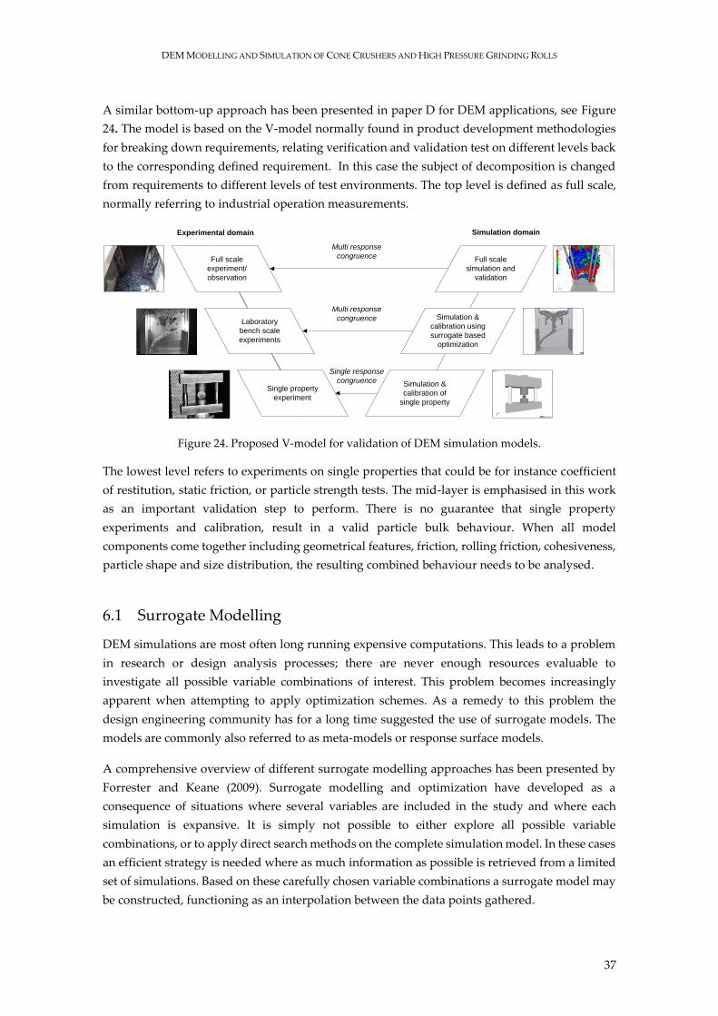
DEM MODELLING AND SIMULATION OF CONE CRUSHERS AND HIGH PRESSURE GRINDING ROLLS
37
A similar bottom-up approach has been presented in paper D for DEM applications, see Figure
24. The model is based on the V-model normally found in product development methodologies
for breaking down requirements, relating verification and validation test on different levels back
to the corresponding defined requirement. In this case the subject of decomposition is changed
from requirements to different levels of test environments. The top level is defined as full scale,
normally referring to industrial operation measurements.
Figure 24. Proposed V-model for validation of DEM simulation models.
The lowest level refers to experiments on single properties that could be for instance coefficient
of restitution, static friction, or particle strength tests. The mid-layer is emphasised in this work
as an important validation step to perform. There is no guarantee that single property
experiments and calibration, result in a valid particle bulk behaviour. When all model
components come together including geometrical features, friction, rolling friction, cohesiveness,
particle shape and size distribution, the resulting combined behaviour needs to be analysed.
6.1 Surrogate Modelling
DEM simulations are most often long running expensive computations. This leads to a problem
in research or design analysis processes; there are never enough resources evaluable to
investigate all possible variable combinations of interest. This problem becomes increasingly
apparent when attempting to apply optimization schemes. As a remedy to this problem the
design engineering community has for a long time suggested the use of surrogate models. The
models are commonly also referred to as meta-models or response surface models.
A comprehensive overview of different surrogate modelling approaches has been presented by
Forrester and Keane (2009). Surrogate modelling and optimization have developed as a
consequence of situations where several variables are included in the study and where each
simulation is expansive. It is simply not possible to either explore all possible variable
combinations, or to apply direct search methods on the complete simulation model. In these cases
an efficient strategy is needed where as much information as possible is retrieved from a limited
set of simulations. Based on these carefully chosen variable combinations a surrogate model may
be constructed, functioning as an interpolation between the data points gathered.
Simulation domainExperimental domain
Full scale
experiment/
observation
Full scale
simulation and
validation
Laboratory
bench scale
experiments
Simulation &
calibration using
surrogate based
optimization
Single property
experiment
Simulation &
calibration of
single property
Single response
congruence
Multi response
congruence
Multi response
congruence
JOHANNES QUIST
38
The first step in the response modelling process is to decide what parameters to explore and vary
- in other words the variables. In some cases this choice may be obvious, however in many
situations the first question is more targeted towards what parameters influence what responses.
These relationships may be analysed and determined by performing sensitivity analysis (in some
cases called statistical screening analysis) using design of experiments. Experimental plans such
as for instance fractional factorial designs or Placket Burman designs are efficient while they have
the inherent drawback of sacrificing information regarding higher order variable interactions
(Box, 2005). These designs are useful in order to bring clarity regarding;
1. What variables have a statistically provable effect on what response variables?
2. From the identified significant variables, which ones are the most influential and which
variable interactions are active?
The modeller needs to understand these relationships before proceeding with response
modelling. In some cases these relationships may be already known a priori and the modeller
may directly focus on experimental designs more suitable for response modelling. The response
surface modelling experimental design may be developed as an extension of the screening design,
or, a new separate experimental design dedicated for response modelling is created. The
extension of an existing experimental plan can be realised through the concept of design
augmentation (SAS Institute, 2015) (called sequential assembly in Box (2005)). The augmentation
enables a controlled way of expanding the design plan while maintaining each variable column
mutually orthogonal. Variable column vectors are mutually orthogonal if the sum of the products
of their corresponding elements is 0. Orthogonality is important in design of experiments since it
allows for analysis of main effects and interactions independently.
The four most common experimental plans for response surface modelling are shown in Figure
25. The full factorial design (here presented as a 25 design) is perhaps the easiest to apply and
understand. A more efficient space filling design is the Latin Hypercube design, in this example
displayed using 20 points. In contrast to the full factorial design the Latin Hypercube is based on
defining how many experiments that should be performed. The algorithm then positions the
points in order to achieve an optimal spacing and filling. The central composite design (CCD)
expands the full factorial design with a centre and star points (Box, 2005). The Box-Behnken
design is an incomplete three-level factorial design where the points are specifically chosen to
allow efficient estimation of coefficients for second order polynomial models. Points are not
positioned in the corners however, instead they are inserted on the midpoints of each edge of the
experimental space.
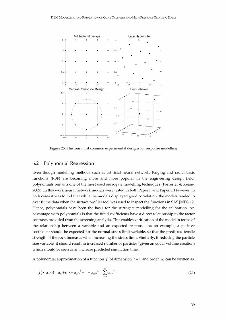
DEM MODELLING AND SIMULATION OF CONE CRUSHERS AND HIGH PRESSURE GRINDING ROLLS
39
Figure 25. The four most common experimental designs for response modelling
6.2 Polynomial Regression
Even though modelling methods such as artificial neural network, Kriging and radial basis
functions (RBF) are becoming more and more popular in the engineering design field,
polynomials remains one of the most used surrogate modelling techniques (Forrester & Keane,
2009). In this work neural network models were tested in both Paper F and Paper I. However, in
both cases it was found that while the models displayed good correlation, the models tended to
over fit the data when the surface profiler tool was used to inspect the functions in SAS JMP® 12.
Hence, polynomials have been the basis for the surrogate modelling for the calibration. An
advantage with polynomials is that the fitted coefficients have a direct relationship to the factor
contrasts provided from the screening analysis. This enables verification of the model in terms of
the relationship between a variable and an expected response. As an example, a positive
coefficient should be expected for the normal stress limit variable, so that the predicted tensile
strength of the rock increases when increasing the stress limit. Similarly, if reducing the particle
size variable, it should result in increased number of particles (given an equal volume creation)
which should be seen as an increase predicted simulation time.
A polynomial approximation of a function f of dimension 1n and order m , can be written as,
2 ( )
0 1 2
0
ˆ , , ...m
m i
m i
i
y x m x x x x
(24)
0.5
1
-0.5
-1
0
0 0.5-0.5-1 1
0.5
1
-0.5
-1
0
0 0.5-0.5-1 1
Full factorial design Latin Hypercube
Central Composite Design Box-Behnken
1
1.5
-1
-1.5
0
0 1-1-1.5 1.5
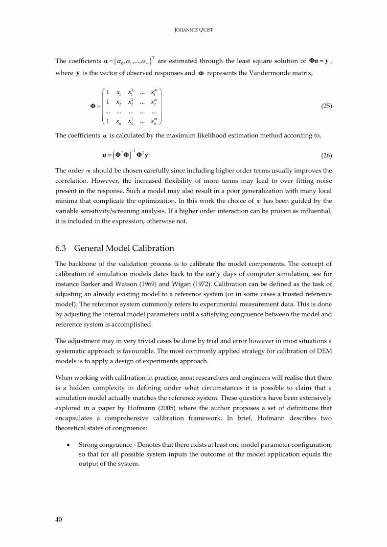
JOHANNES QUIST
40
The coefficients T
0 1, ,..., m α are estimated through the least square solution of Φα y ,
where y is the vector of observed responses and Φ represents the Vandermonde matrix,
2
1 1 1
2
2 2 2
2
1 ...
1 ...
... ... ... ... ...
1 ...
m
m
m
n n n
x x x
x x x
x x x
Φ (25)
The coefficients α is calculated by the maximum likelihood estimation method according to,
1
T T
α Φ Φ Φ y (26)
The order m should be chosen carefully since including higher order terms usually improves the
correlation. However, the increased flexibility of more terms may lead to over fitting noise
present in the response. Such a model may also result in a poor generalization with many local
minima that complicate the optimization. In this work the choice of m has been guided by the
variable sensitivity/screening analysis. If a higher order interaction can be proven as influential,
it is included in the expression, otherwise not.
6.3 General Model Calibration
The backbone of the validation process is to calibrate the model components. The concept of
calibration of simulation models dates back to the early days of computer simulation, see for
instance Barker and Watson (1969) and Wigan (1972). Calibration can be defined as the task of
adjusting an already existing model to a reference system (or in some cases a trusted reference
model). The reference system commonly refers to experimental measurement data. This is done
by adjusting the internal model parameters until a satisfying congruence between the model and
reference system is accomplished.
The adjustment may in very trivial cases be done by trial and error however in most situations a
systematic approach is favourable. The most commonly applied strategy for calibration of DEM
models is to apply a design of experiments approach.
When working with calibration in practice, most researchers and engineers will realise that there
is a hidden complexity in defining under what circumstances it is possible to claim that a
simulation model actually matches the reference system. These questions have been extensively
explored in a paper by Hofmann (2005) where the author proposes a set of definitions that
encapsulates a comprehensive calibration framework. In brief, Hofmann describes two
theoretical states of congruence:
Strong congruence - Denotes that there exists at least one model parameter configuration,
so that for all possible system inputs the outcome of the model application equals the
output of the system.
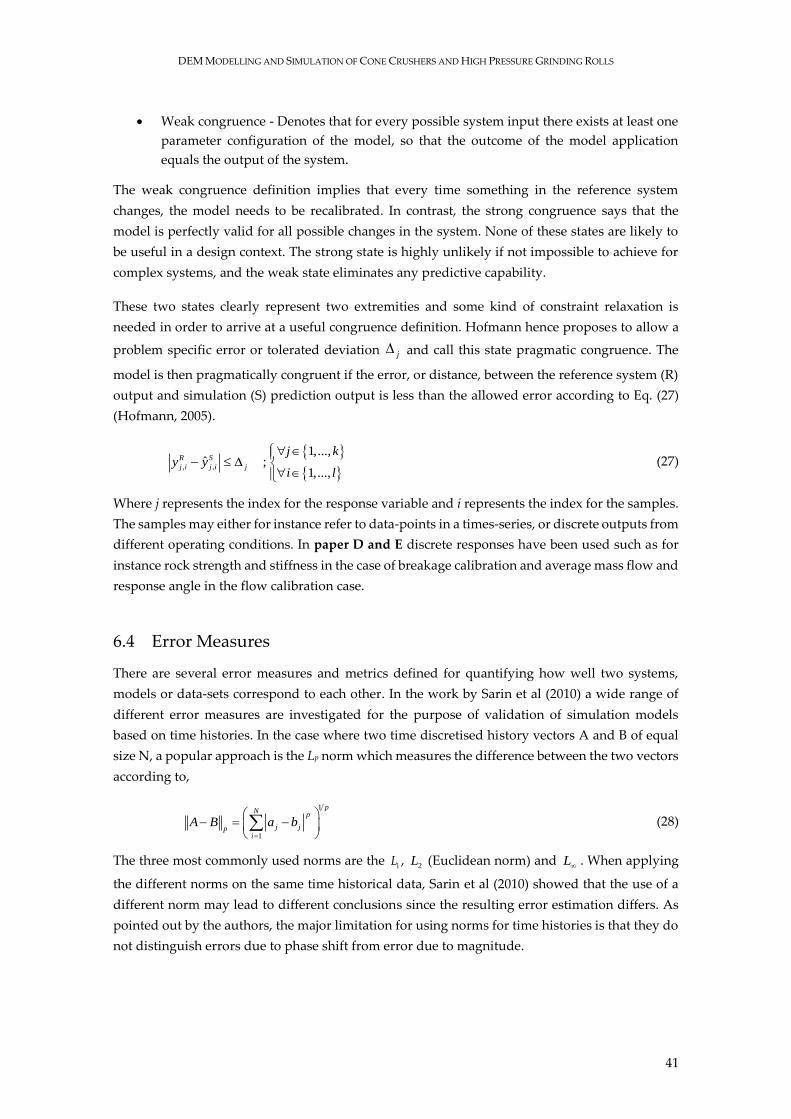
DEM MODELLING AND SIMULATION OF CONE CRUSHERS AND HIGH PRESSURE GRINDING ROLLS
41
Weak congruence - Denotes that for every possible system input there exists at least one
parameter configuration of the model, so that the outcome of the model application
equals the output of the system.
The weak congruence definition implies that every time something in the reference system
changes, the model needs to be recalibrated. In contrast, the strong congruence says that the
model is perfectly valid for all possible changes in the system. None of these states are likely to
be useful in a design context. The strong state is highly unlikely if not impossible to achieve for
complex systems, and the weak state eliminates any predictive capability.
These two states clearly represent two extremities and some kind of constraint relaxation is
needed in order to arrive at a useful congruence definition. Hofmann hence proposes to allow a
problem specific error or tolerated deviation j and call this state pragmatic congruence. The
model is then pragmatically congruent if the error, or distance, between the reference system (R)
output and simulation (S) prediction output is less than the allowed error according to Eq. (27)
(Hofmann, 2005).
, ,
1,...,ˆ ;
1,...,
R S
j i j i j
j ky y
i l
(27)
Where j represents the index for the response variable and i represents the index for the samples.
The samples may either for instance refer to data-points in a times-series, or discrete outputs from
different operating conditions. In paper D and E discrete responses have been used such as for
instance rock strength and stiffness in the case of breakage calibration and average mass flow and
response angle in the flow calibration case.
6.4 Error Measures
There are several error measures and metrics defined for quantifying how well two systems,
models or data-sets correspond to each other. In the work by Sarin et al (2010) a wide range of
different error measures are investigated for the purpose of validation of simulation models
based on time histories. In the case where two time discretised history vectors A and B of equal
size N, a popular approach is the Lp norm which measures the difference between the two vectors
according to,
1
1
pN
p
j jpi
A B a b
(28)
The three most commonly used norms are the 1L , 2L (Euclidean norm) and L . When applying
the different norms on the same time historical data, Sarin et al (2010) showed that the use of a
different norm may lead to different conclusions since the resulting error estimation differs. As
pointed out by the authors, the major limitation for using norms for time histories is that they do
not distinguish errors due to phase shift from error due to magnitude.
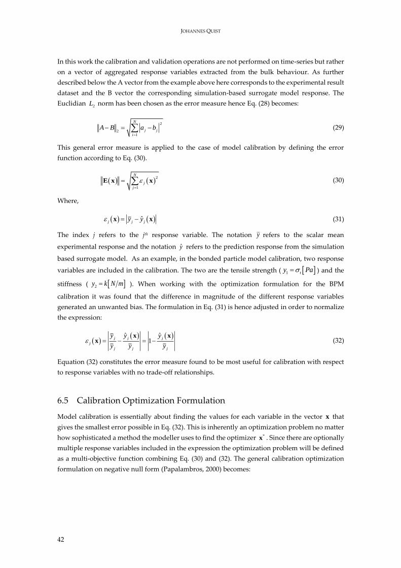
JOHANNES QUIST
42
In this work the calibration and validation operations are not performed on time-series but rather
on a vector of aggregated response variables extracted from the bulk behaviour. As further
described below the A vector from the example above here corresponds to the experimental result
dataset and the B vector the corresponding simulation-based surrogate model response. The
Euclidian 2L norm has been chosen as the error measure hence Eq. (28) becomes:
2
21
N
j j
i
A B a b
(29)
This general error measure is applied to the case of model calibration by defining the error
function according to Eq. (30).
2
1
N
j
j
E x x (30)
Where,
ˆj j jy y x x (31)
The index j refers to the jth response variable. The notation y refers to the scalar mean
experimental response and the notation y refers to the prediction response from the simulation
based surrogate model. As an example, in the bonded particle model calibration, two response
variables are included in the calibration. The two are the tensile strength ( 1 ty Pa ) and the
stiffness ( 2y k N m ). When working with the optimization formulation for the BPM
calibration it was found that the difference in magnitude of the different response variables
generated an unwanted bias. The formulation in Eq. (31) is hence adjusted in order to normalize
the expression:
ˆ ˆ
1j j j
j
j j j
y y y
y y y
x xx (32)
Equation (32) constitutes the error measure found to be most useful for calibration with respect
to response variables with no trade-off relationships.
6.5 Calibration Optimization Formulation
Model calibration is essentially about finding the values for each variable in the vector x that
gives the smallest error possible in Eq. (32). This is inherently an optimization problem no matter
how sophisticated a method the modeller uses to find the optimizer *x . Since there are optionally
multiple response variables included in the expression the optimization problem will be defined
as a multi-objective function combining Eq. (30) and (32). The general calibration optimization
formulation on negative null form (Papalambros, 2000) becomes:
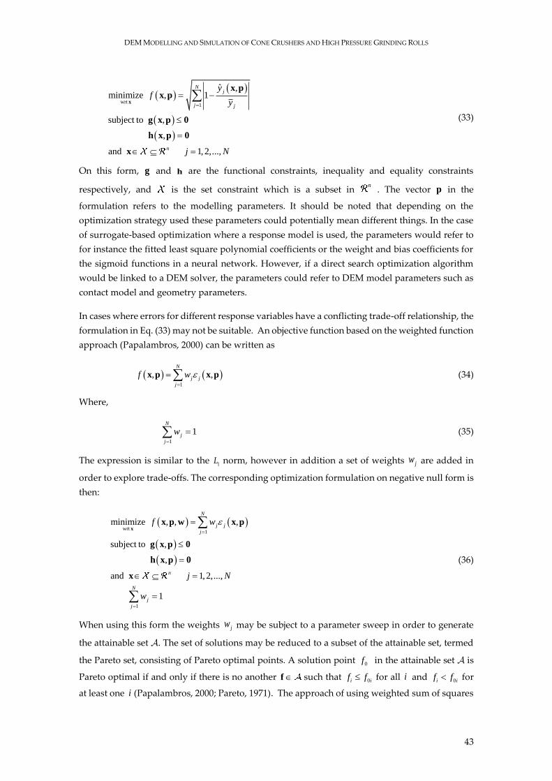
DEM MODELLING AND SIMULATION OF CONE CRUSHERS AND HIGH PRESSURE GRINDING ROLLS
43
wrt1
ˆ ,minimize , 1
subject to ,
,
and 1,2,...,
Nj
j j
n
yf
y
j N
x
x px p
g x p 0
h x p 0
x
(33)
On this form, g and h are the functional constraints, inequality and equality constraints
respectively, and is the set constraint which is a subset in n
. The vector p in the
formulation refers to the modelling parameters. It should be noted that depending on the
optimization strategy used these parameters could potentially mean different things. In the case
of surrogate-based optimization where a response model is used, the parameters would refer to
for instance the fitted least square polynomial coefficients or the weight and bias coefficients for
the sigmoid functions in a neural network. However, if a direct search optimization algorithm
would be linked to a DEM solver, the parameters could refer to DEM model parameters such as
contact model and geometry parameters.
In cases where errors for different response variables have a conflicting trade-off relationship, the
formulation in Eq. (33) may not be suitable. An objective function based on the weighted function
approach (Papalambros, 2000) can be written as
1
, ,N
j j
j
f w
x p x p (34)
Where,
1
1N
j
j
w
(35)
The expression is similar to the 1L norm, however in addition a set of weights jw are added in
order to explore trade-offs. The corresponding optimization formulation on negative null form is
then:
wrt1
1
minimize , , ,
subject to ,
,
and 1,2,...,
1
N
j j
j
n
N
j
j
f w
j N
w
xx p w x p
g x p 0
h x p 0
x
(36)
When using this form the weights jw may be subject to a parameter sweep in order to generate
the attainable set . The set of solutions may be reduced to a subset of the attainable set, termed
the Pareto set, consisting of Pareto optimal points. A solution point 0f in the attainable set is
Pareto optimal if and only if there is no another f such that 0i if f for all i and 0i if f for
at least one i (Papalambros, 2000; Pareto, 1971). The approach of using weighted sum of squares
JOHANNES QUIST
44
has previously been applied for calibration of contact model parameters by Kruggel-Emden
(Kruggel-Emden et al., 2007).
6.6 Bonded Particle Model Calibration
In order for a breakage model to be useful in a machine simulation setting it needs to be calibrated
against experimental data; regardless of the specific choice of modelling approach. Several
studies have contributed to the topic of calibration of DEM models. However they may be divided
into two main areas where the first concerns applications related to granular flow. In this area
several researchers have made important contributions, see for instance (G. K. P. Barrios, de
Carvalho, Kwade, & Tavares, 2013; C. J. Coetzee, 2017; C. J. Coetzee, Els, D.N.J., 2009; C. J. Coetzee
& Nel, 2014; Combarros, Feise, Zetzener, & Kwade, 2014; Favier, 2010; Frankowski et al., 2013;
González-Montellano, Ramírez, Gallego, & Ayuga, 2011; Grima, 2009, 2011; Gröger, 2006; J. Quist,
2015).
In the area of calibrating bonded particle models, Hanley (2011), Yoon (2007), Wang and Tonon
(2009) as well as Jiang et al (2015) have made important advancements by introducing statistical
design of experiment methods and calibration optimization. In the calibration procedure
demonstrated by Wang and Tonon (2009), sensitivity analysis is performed by varying one factor
while fixing the others. This approach is simple and requires few simulations, however the
method does not capture the second and third order interaction relationships between micro
parameters. Even though the researchers succeeded in modelling the breakage behaviour well
for both unconfined uniaxial strength and direct tensile strength tests they concluded that only
two parameters are not sufficient for achieving a good calibration outcome. In the work presented
by Hanley (2011), ANOVA analysis was used to analyse the responses from 3D simulations of
particle agglomerate compression with micro parameters configured by a Taguchi L27 array (27
runs with 13 columns). The results from the study displayed reasonable prediction capabilities
for some of the response variables. It was however concluded that more simulations, hence a
larger experimental design plan, was needed in order to resolve significant factor aliases.
In the work by Yoon (2007) the design of experiments approach is both well described and
applied by using both Placket-Burman (PB) designs for factor screening and Central-Composite
Designs (CCD) for response surface modelling. The proposed approach is based on first applying
a PB screening design in order to evaluate which micro parameters are statistically significant for
each response variable. When this has been done a CCD is created in order to fit response models
for each output response variable. The results show good predictability and correspondence to
experimental data. However, the simulations are performed using 2D DEM code hence it is not
possible to utilize the outcome directly for 3D DEM simulations.
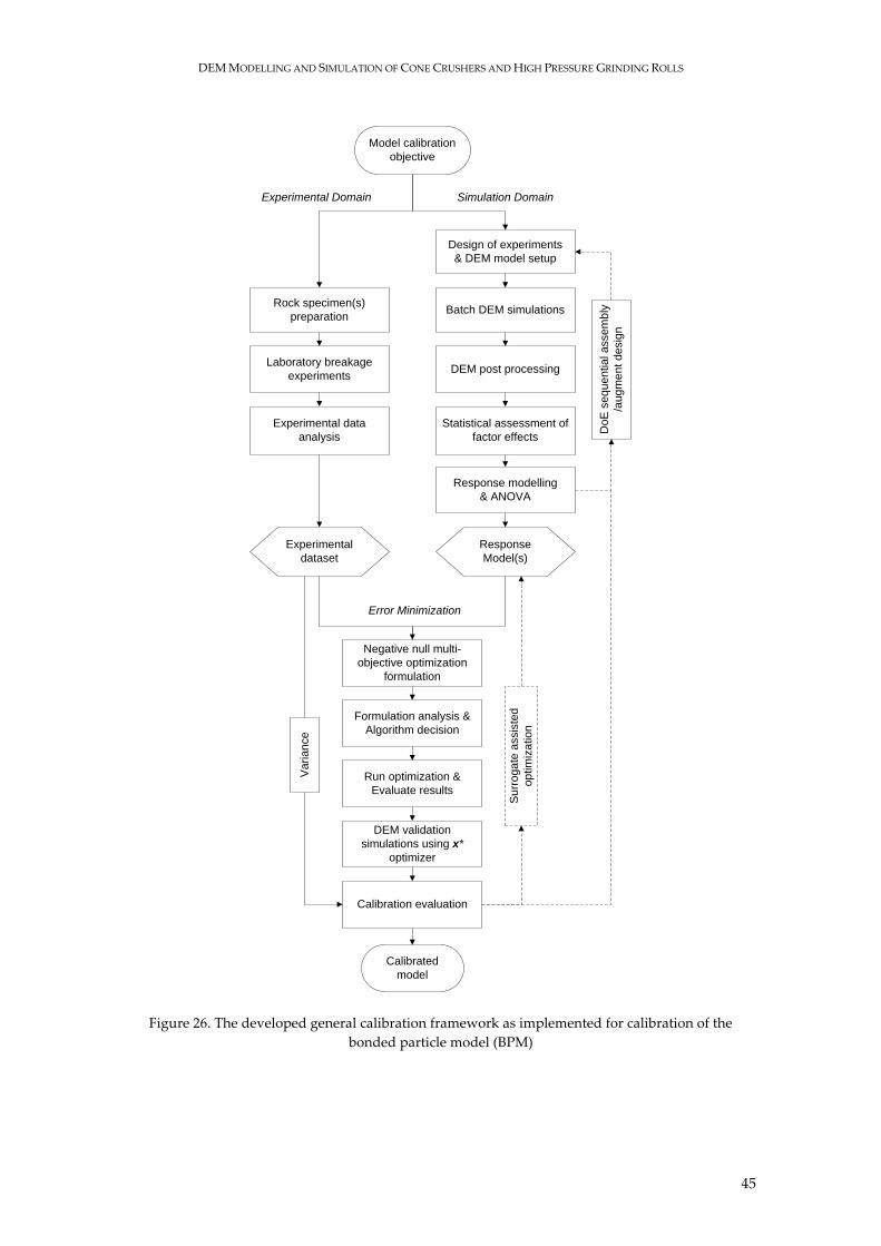
DEM MODELLING AND SIMULATION OF CONE CRUSHERS AND HIGH PRESSURE GRINDING ROLLS
45
Figure 26. The developed general calibration framework as implemented for calibration of the
bonded particle model (BPM)
Run optimization &
Evaluate results
Design of experiments
& DEM model setup
Response modelling
& ANOVA
Batch DEM simulations
Statistical assessment of
factor effects
Negative null multi-
objective optimization
formulation
Formulation analysis &
Algorithm decision
DEM validation
simulations using x*
optimizer
Rock specimen(s)
preparation
Laboratory breakage
experimentsDEM post processing
Experimental data
analysis
Calibration evaluation
Do
E s
eq
ue
ntia
l a
sse
mb
ly
/au
gm
en
t d
esig
n
Model calibration
objective
Calibrated
model
Experimental
dataset
Response
Model(s)
Simulation DomainExperimental Domain
Su
rro
ga
te a
ssis
ted
op
tim
iza
tio
n
Error Minimization
Va
ria
nce
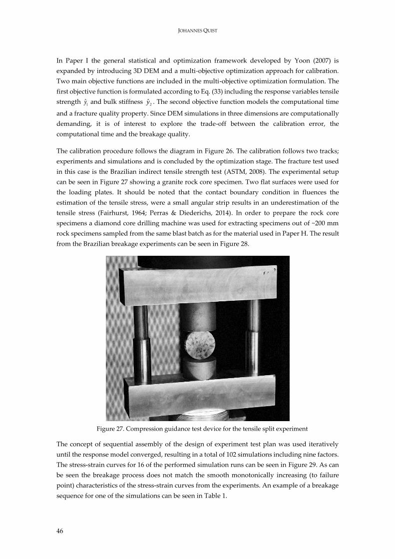
JOHANNES QUIST
46
In Paper I the general statistical and optimization framework developed by Yoon (2007) is
expanded by introducing 3D DEM and a multi-objective optimization approach for calibration.
Two main objective functions are included in the multi-objective optimization formulation. The
first objective function is formulated according to Eq. (33) including the response variables tensile
strength 1y and bulk stiffness
2y . The second objective function models the computational time
and a fracture quality property. Since DEM simulations in three dimensions are computationally
demanding, it is of interest to explore the trade-off between the calibration error, the
computational time and the breakage quality.
The calibration procedure follows the diagram in Figure 26. The calibration follows two tracks;
experiments and simulations and is concluded by the optimization stage. The fracture test used
in this case is the Brazilian indirect tensile strength test (ASTM, 2008). The experimental setup
can be seen in Figure 27 showing a granite rock core specimen. Two flat surfaces were used for
the loading plates. It should be noted that the contact boundary condition in fluences the
estimation of the tensile stress, were a small angular strip results in an underestimation of the
tensile stress (Fairhurst, 1964; Perras & Diederichs, 2014). In order to prepare the rock core
specimens a diamond core drilling machine was used for extracting specimens out of ~200 mm
rock specimens sampled from the same blast batch as for the material used in Paper H. The result
from the Brazilian breakage experiments can be seen in Figure 28.
Figure 27. Compression guidance test device for the tensile split experiment
The concept of sequential assembly of the design of experiment test plan was used iteratively
until the response model converged, resulting in a total of 102 simulations including nine factors.
The stress-strain curves for 16 of the performed simulation runs can be seen in Figure 29. As can
be seen the breakage process does not match the smooth monotonically increasing (to failure
point) characteristics of the stress-strain curves from the experiments. An example of a breakage
sequence for one of the simulations can be seen in Table 1.
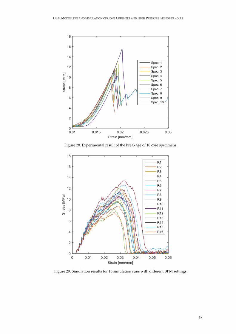
DEM MODELLING AND SIMULATION OF CONE CRUSHERS AND HIGH PRESSURE GRINDING ROLLS
47
Figure 28. Experimental result of the breakage of 10 core specimens.
Figure 29. Simulation results for 16 simulation runs with different BPM settings.
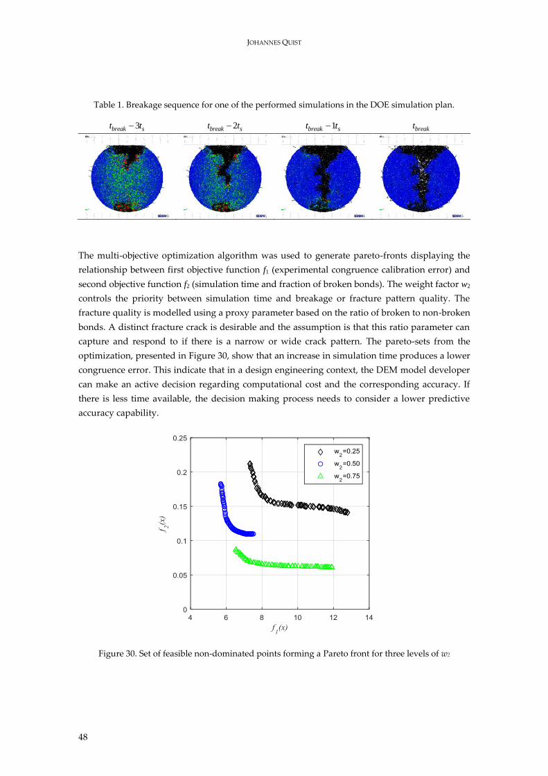
JOHANNES QUIST
48
Table 1. Breakage sequence for one of the performed simulations in the DOE simulation plan.
3break st t 2break st t 1break st t breakt
The multi-objective optimization algorithm was used to generate pareto-fronts displaying the
relationship between first objective function f1 (experimental congruence calibration error) and
second objective function f2 (simulation time and fraction of broken bonds). The weight factor w2
controls the priority between simulation time and breakage or fracture pattern quality. The
fracture quality is modelled using a proxy parameter based on the ratio of broken to non-broken
bonds. A distinct fracture crack is desirable and the assumption is that this ratio parameter can
capture and respond to if there is a narrow or wide crack pattern. The pareto-sets from the
optimization, presented in Figure 30, show that an increase in simulation time produces a lower
congruence error. This indicate that in a design engineering context, the DEM model developer
can make an active decision regarding computational cost and the corresponding accuracy. If
there is less time available, the decision making process needs to consider a lower predictive
accuracy capability.
Figure 30. Set of feasible non-dominated points forming a Pareto front for three levels of w2
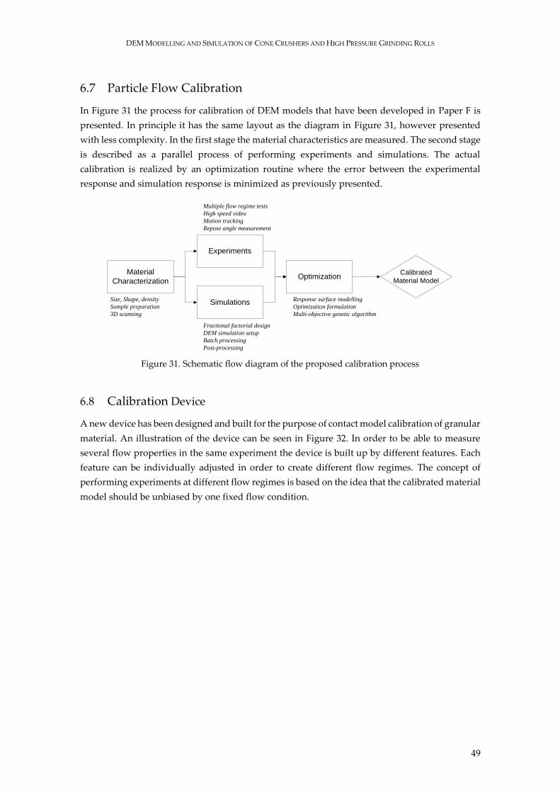
DEM MODELLING AND SIMULATION OF CONE CRUSHERS AND HIGH PRESSURE GRINDING ROLLS
49
6.7 Particle Flow Calibration
In Figure 31 the process for calibration of DEM models that have been developed in Paper F is
presented. In principle it has the same layout as the diagram in Figure 31, however presented
with less complexity. In the first stage the material characteristics are measured. The second stage
is described as a parallel process of performing experiments and simulations. The actual
calibration is realized by an optimization routine where the error between the experimental
response and simulation response is minimized as previously presented.
Figure 31. Schematic flow diagram of the proposed calibration process
6.8 Calibration Device
A new device has been designed and built for the purpose of contact model calibration of granular
material. An illustration of the device can be seen in Figure 32. In order to be able to measure
several flow properties in the same experiment the device is built up by different features. Each
feature can be individually adjusted in order to create different flow regimes. The concept of
performing experiments at different flow regimes is based on the idea that the calibrated material
model should be unbiased by one fixed flow condition.
Size, Shape, density
Sample preparation
3D scanning
Fractional factorial design
DEM simulation setup
Batch processing
Post-processing
Multiple flow regime tests
High speed video
Motion tracking
Repose angle measurement
Response surface modelling
Optimization formulation
Multi-objective genetic algorithm
Material
CharacterizationOptimization
Experiments
Simulations
Calibrated
Material Model
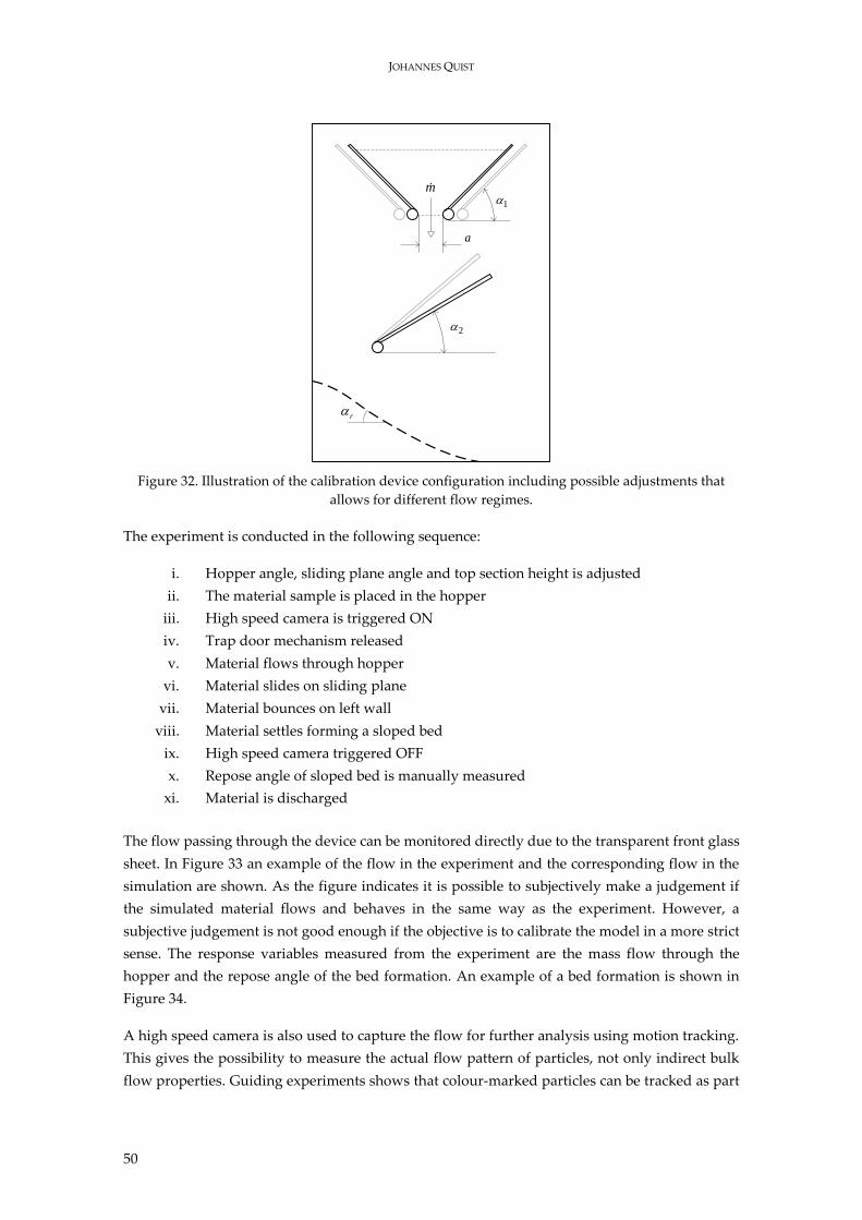
JOHANNES QUIST
50
Figure 32. Illustration of the calibration device configuration including possible adjustments that
allows for different flow regimes.
The experiment is conducted in the following sequence:
i. Hopper angle, sliding plane angle and top section height is adjusted
ii. The material sample is placed in the hopper
iii. High speed camera is triggered ON
iv. Trap door mechanism released
v. Material flows through hopper
vi. Material slides on sliding plane
vii. Material bounces on left wall
viii. Material settles forming a sloped bed
ix. High speed camera triggered OFF
x. Repose angle of sloped bed is manually measured
xi. Material is discharged
The flow passing through the device can be monitored directly due to the transparent front glass
sheet. In Figure 33 an example of the flow in the experiment and the corresponding flow in the
simulation are shown. As the figure indicates it is possible to subjectively make a judgement if
the simulated material flows and behaves in the same way as the experiment. However, a
subjective judgement is not good enough if the objective is to calibrate the model in a more strict
sense. The response variables measured from the experiment are the mass flow through the
hopper and the repose angle of the bed formation. An example of a bed formation is shown in
Figure 34.
A high speed camera is also used to capture the flow for further analysis using motion tracking.
This gives the possibility to measure the actual flow pattern of particles, not only indirect bulk
flow properties. Guiding experiments shows that colour-marked particles can be tracked as part
m
r
2
1
a
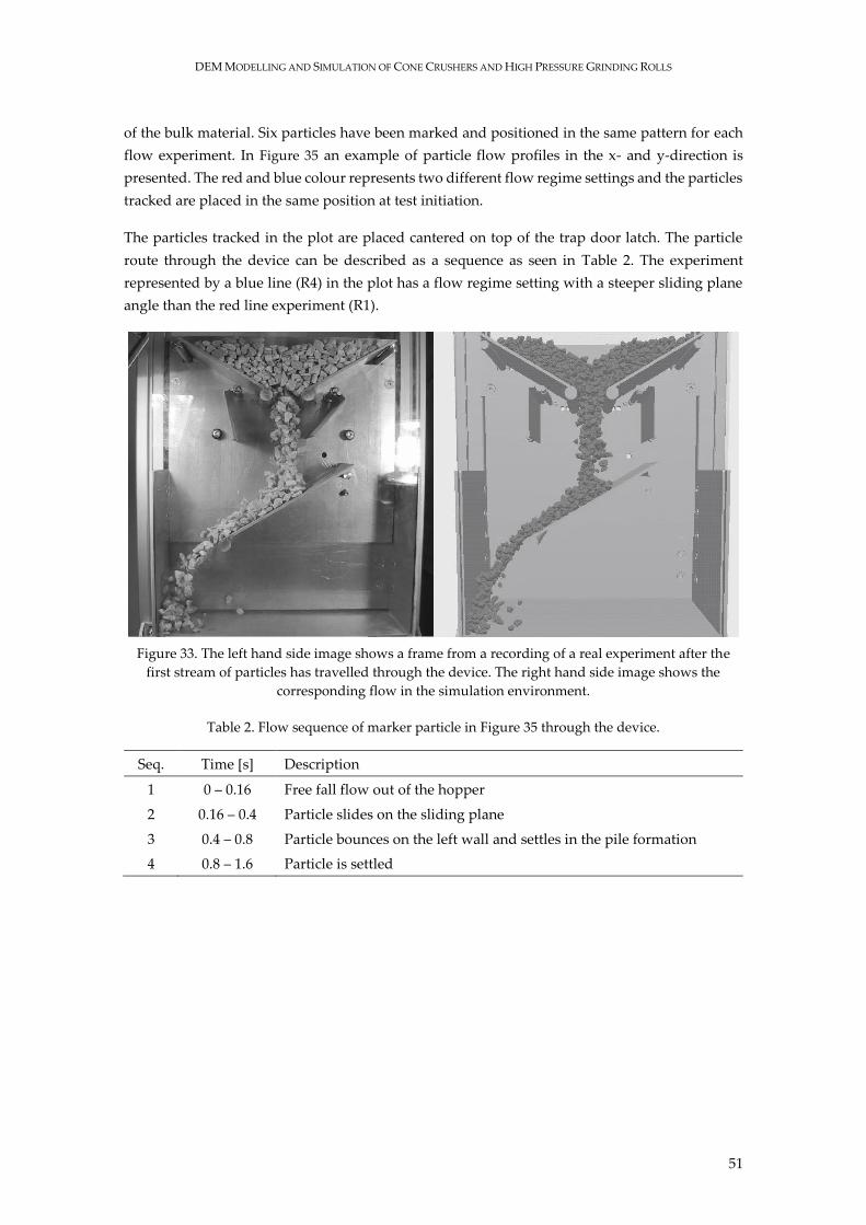
DEM MODELLING AND SIMULATION OF CONE CRUSHERS AND HIGH PRESSURE GRINDING ROLLS
51
of the bulk material. Six particles have been marked and positioned in the same pattern for each
flow experiment. In Figure 35 an example of particle flow profiles in the x- and y-direction is
presented. The red and blue colour represents two different flow regime settings and the particles
tracked are placed in the same position at test initiation.
The particles tracked in the plot are placed cantered on top of the trap door latch. The particle
route through the device can be described as a sequence as seen in Table 2. The experiment
represented by a blue line (R4) in the plot has a flow regime setting with a steeper sliding plane
angle than the red line experiment (R1).
Figure 33. The left hand side image shows a frame from a recording of a real experiment after the
first stream of particles has travelled through the device. The right hand side image shows the
corresponding flow in the simulation environment.
Table 2. Flow sequence of marker particle in Figure 35 through the device.
Seq. Time [s] Description
1 0 – 0.16 Free fall flow out of the hopper
2 0.16 – 0.4 Particle slides on the sliding plane
3 0.4 – 0.8 Particle bounces on the left wall and settles in the pile formation
4 0.8 – 1.6 Particle is settled
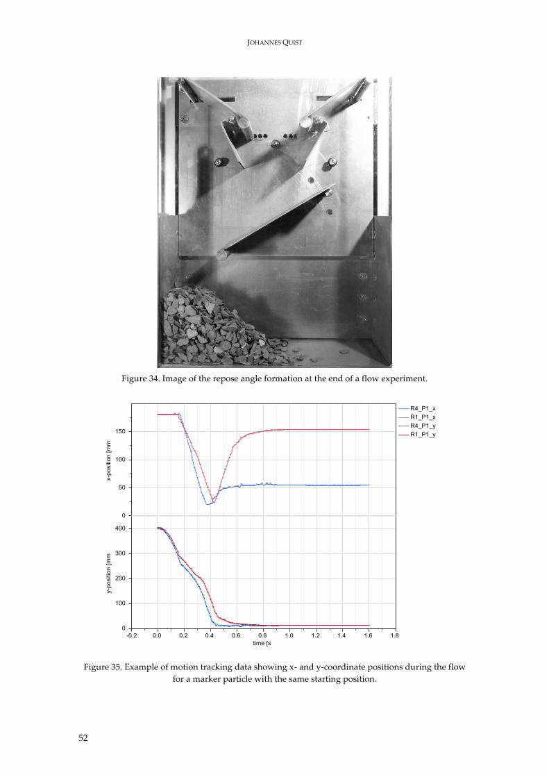
JOHANNES QUIST
52
Figure 34. Image of the repose angle formation at the end of a flow experiment.
Figure 35. Example of motion tracking data showing x- and y-coordinate positions during the flow
for a marker particle with the same starting position.
DEM MODELLING AND SIMULATION OF CONE CRUSHERS AND HIGH PRESSURE GRINDING ROLLS
53
The developed method for direct measurement of the particle flow is promising and gives a good
subjective understanding. However, so far the method has not been developed far enough to
enable a statistical comparison to simulation data. One identified issue is that the random
variance in the trajectories was high due to the particle shape, initial starting positions and
orientation of particles in both the simulation and experimental case. In order to utilize the high-
fidelity trajectory data, a higher level of automated data analysis for both motion tracking
trajectory data and simulation trajectory data is needed. Due to this reason the bulk flow
measures in terms of mass flow and repose angle was used as response variables for the
calibration.
The calibration outcome using the device and process have been successful in terms of calibrating
size, shape, static friction and rolling friction. However, it was found that the coefficient of
restitution did not have a statistically significant effect on the mass flow and repose angle
response variables. When analysing the simulation results it was found that the coefficient of
restitution clearly affected the flow behaviour, however mostly in the interaction with the sliding
plane and most importantly with the left wall. Hence, in order to improve the calibration method
an idea would be to utilize the trajectory data. If an algorithm could identify a set of particle-
particle and particle-wall collisions, the velocities before and after the collisions could be
calculated, providing a data-set where the restitution behaviour is captured with a good statistical
basis. Using this data, an estimate of the average coefficient of restitution could possibly be
calculated.

JOHANNES QUIST
54
DEM MODELLING AND SIMULATION OF CONE CRUSHERS AND HIGH PRESSURE GRINDING ROLLS
55
7 Cone Crusher Modelling
7.1 Cone Crusher Eccentric Speed
The research objective for the study in Paper A was to investigate the influence of eccentric speed
on the crusher capacity. The BPM was used to bond together fraction particles to meta-particles
with the shape of spheres. The spherical shape of the meta-particles is of course not representative
of the irregularly shaped rock particles normally feeding a crusher. However, the simplistic shape
results in distinct and distilled flow behaviour that is of interest when looking at the principle
dynamics of the particles in the crushing chamber.
Evertsson (1999) established an analytical framework for modelling flow of particles in a cone
crusher. From this work it can be derived that if the eccentric speed is increased the number of
breakage zones and events will increase. The obvious reason is that the mantle will interact with
the particles more frequently. Further on, particles will have less time to accelerate and move
down the chamber between each compression event.
Five different eccentric speed settings were evaluated by simulating a 40 degree section fed by a
batch of BPM meta-particles. The crusher type was a Sandvik CH430 equipped with a fine
chamber, 12 mm close side setting and 36 mm eccentric throw. The eccentric speed was varied
from 269 to 579 rpm. In Figure 36 an image from the 269 rpm simulation is shown.
In Figure 37 two detail images of the crushing chamber are presented. The left image shows the
particle trajectory of a randomly chosen fraction particle. The trajectory path suggests that the
particle has been subjected to at least 4-5 compressions before leaving the chamber. An important
feature of the trajectory is that the direction of the particle is sometimes turning back upwards.
The effect of a particle moving upwards during compression instead of getting broken is referred
to as squeezing by Evertsson (2000).
In the image to the right the particles in the chamber are represented by bonding beams. From
this view as well from the view in Figure 36, it can be seen that below the choke level, only single
particle breakage occurs. An important qualitative simulation result is that meta-particles break
apart sequentially. In the early phases in this work it proved to be difficult to find a simulation
setup where particles didn’t break apart totally during the first compression. The successful
modelling of sequential breakage is one of the key findings in Paper A.
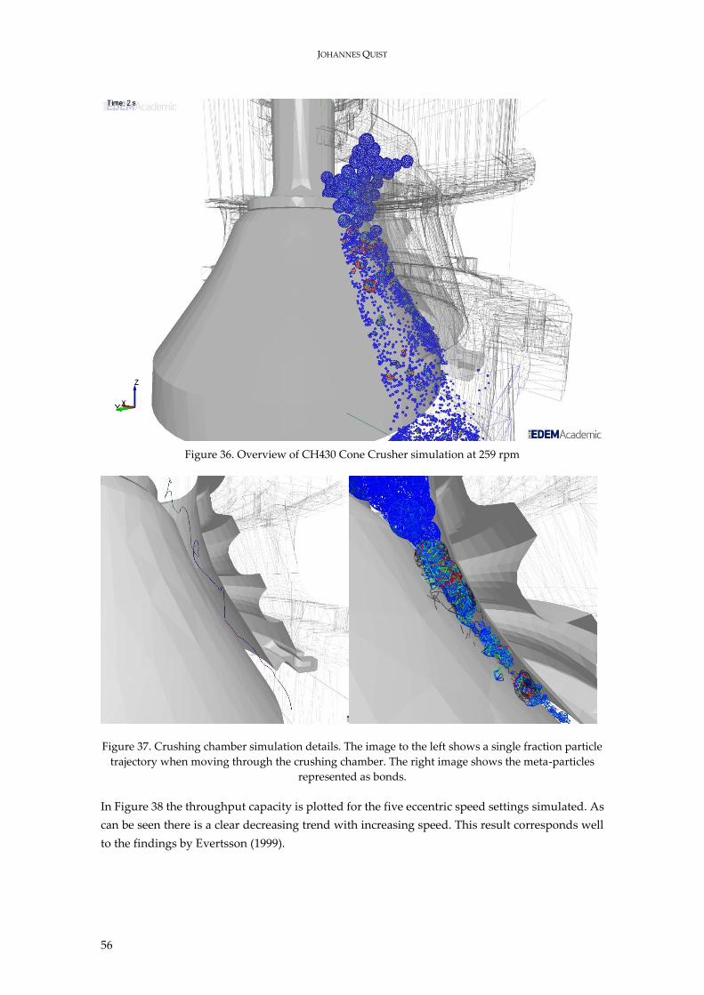
JOHANNES QUIST
56
Figure 36. Overview of CH430 Cone Crusher simulation at 259 rpm
Figure 37. Crushing chamber simulation details. The image to the left shows a single fraction particle
trajectory when moving through the crushing chamber. The right image shows the meta-particles
represented as bonds.
In Figure 38 the throughput capacity is plotted for the five eccentric speed settings simulated. As
can be seen there is a clear decreasing trend with increasing speed. This result corresponds well
to the findings by Evertsson (1999).
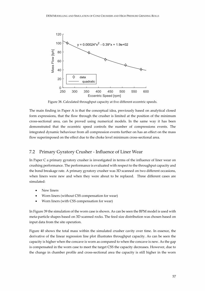
DEM MODELLING AND SIMULATION OF CONE CRUSHERS AND HIGH PRESSURE GRINDING ROLLS
57
Figure 38. Calculated throughput capacity at five different eccentric speeds.
The main finding in Paper A is that the conceptual idea, previously based on analytical closed
form expressions, that the flow through the crusher is limited at the position of the minimum
cross-sectional area, can be proved using numerical models. In the same way it has been
demonstrated that the eccentric speed controls the number of compressions events. The
integrated dynamic behaviour from all compression events further on has an effect on the mass
flow superimposed on the effect due to the choke level minimum cross-sectional area.
7.2 Primary Gyratory Crusher - Influence of Liner Wear
In Paper C a primary gyratory crusher is investigated in terms of the influence of liner wear on
crushing performance. The performance is evaluated with respect to the throughput capacity and
the bond breakage rate. A primary gyratory crusher was 3D scanned on two different occasions,
when liners were new and when they were about to be replaced. Three different cases are
simulated:
New liners
Worn liners (without CSS compensation for wear)
Worn liners (with CSS compensation for wear)
In Figure 39 the simulation of the worn case is shown. As can be seen the BPM model is used with
meta-particle shapes based on 3D scanned rocks. The feed size distribution was chosen based on
input data from the site operation.
Figure 40 shows the total mass within the simulated crusher cavity over time. In essence, the
derivative of the linear regression line plot illustrates throughput capacity. As can be seen the
capacity is higher when the concave is worn as compared to when the concave is new. As the gap
is compensated in the worn case to meet the target CSS the capacity decreases. However, due to
the change in chamber profile and cross-sectional area the capacity is still higher in the worn
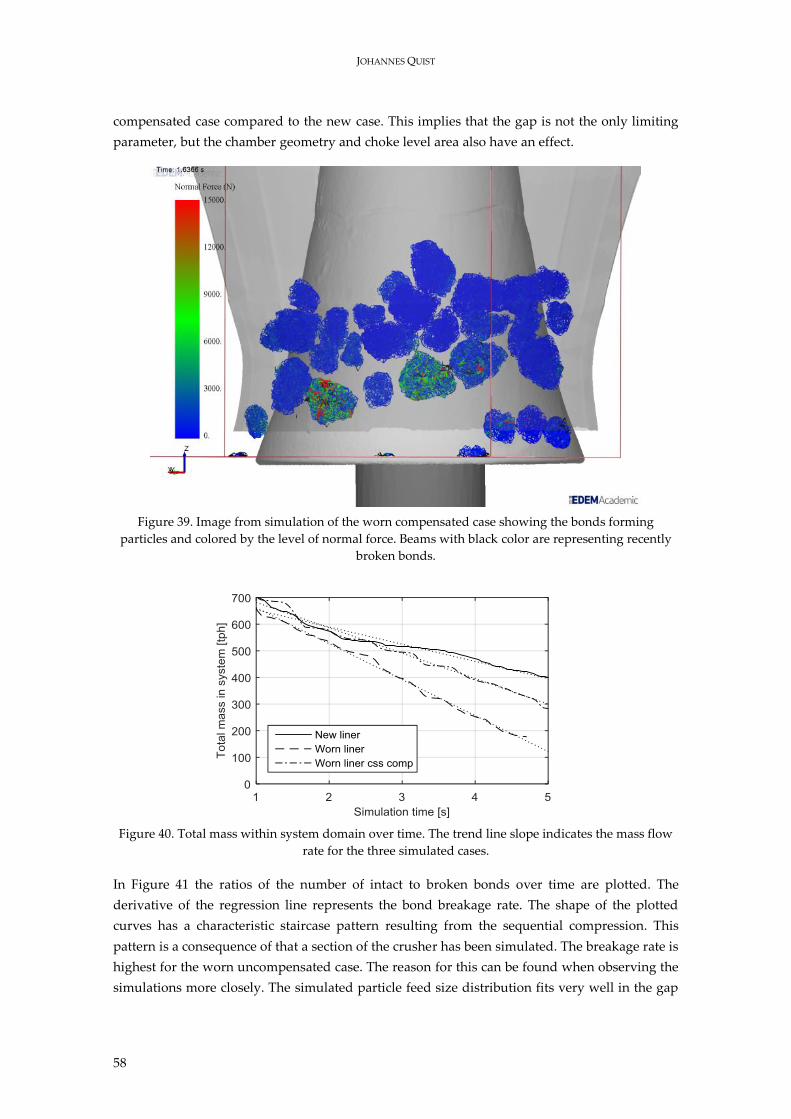
JOHANNES QUIST
58
compensated case compared to the new case. This implies that the gap is not the only limiting
parameter, but the chamber geometry and choke level area also have an effect.
Figure 39. Image from simulation of the worn compensated case showing the bonds forming
particles and colored by the level of normal force. Beams with black color are representing recently
broken bonds.
Figure 40. Total mass within system domain over time. The trend line slope indicates the mass flow
rate for the three simulated cases.
In Figure 41 the ratios of the number of intact to broken bonds over time are plotted. The
derivative of the regression line represents the bond breakage rate. The shape of the plotted
curves has a characteristic staircase pattern resulting from the sequential compression. This
pattern is a consequence of that a section of the crusher has been simulated. The breakage rate is
highest for the worn uncompensated case. The reason for this can be found when observing the
simulations more closely. The simulated particle feed size distribution fits very well in the gap
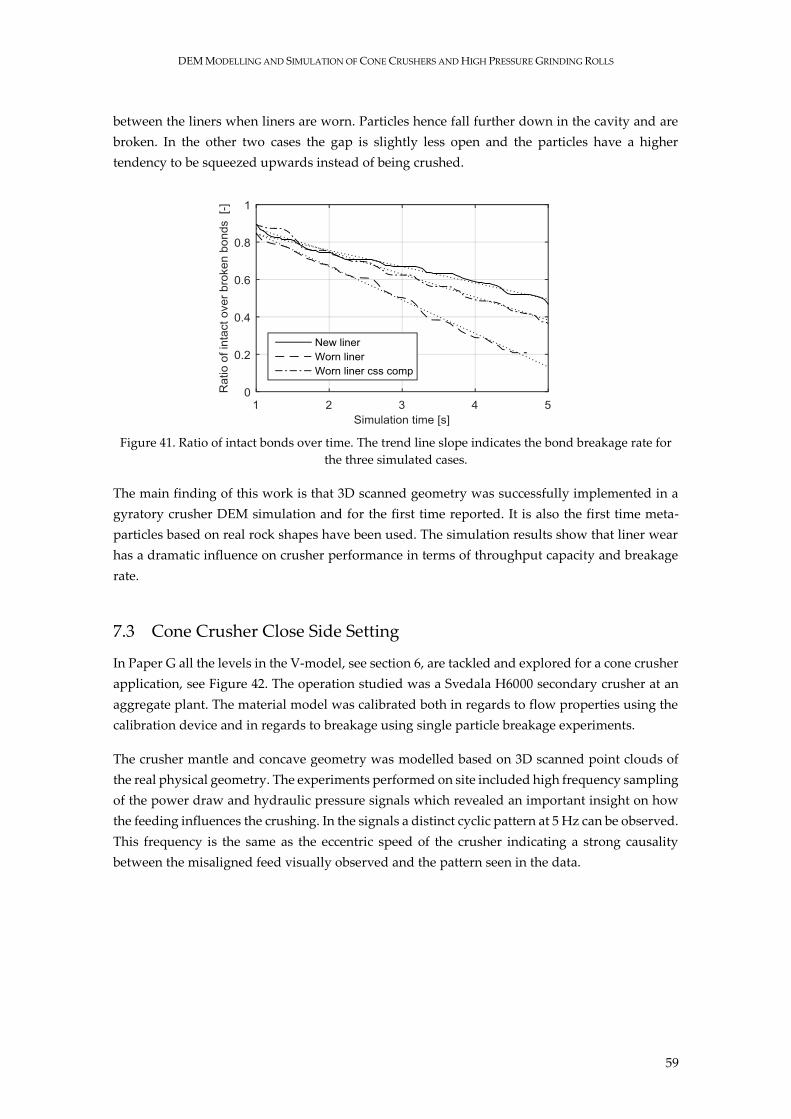
DEM MODELLING AND SIMULATION OF CONE CRUSHERS AND HIGH PRESSURE GRINDING ROLLS
59
between the liners when liners are worn. Particles hence fall further down in the cavity and are
broken. In the other two cases the gap is slightly less open and the particles have a higher
tendency to be squeezed upwards instead of being crushed.
Figure 41. Ratio of intact bonds over time. The trend line slope indicates the bond breakage rate for
the three simulated cases.
The main finding of this work is that 3D scanned geometry was successfully implemented in a
gyratory crusher DEM simulation and for the first time reported. It is also the first time meta-
particles based on real rock shapes have been used. The simulation results show that liner wear
has a dramatic influence on crusher performance in terms of throughput capacity and breakage
rate.
7.3 Cone Crusher Close Side Setting
In Paper G all the levels in the V-model, see section 6, are tackled and explored for a cone crusher
application, see Figure 42. The operation studied was a Svedala H6000 secondary crusher at an
aggregate plant. The material model was calibrated both in regards to flow properties using the
calibration device and in regards to breakage using single particle breakage experiments.
The crusher mantle and concave geometry was modelled based on 3D scanned point clouds of
the real physical geometry. The experiments performed on site included high frequency sampling
of the power draw and hydraulic pressure signals which revealed an important insight on how
the feeding influences the crushing. In the signals a distinct cyclic pattern at 5 Hz can be observed.
This frequency is the same as the eccentric speed of the crusher indicating a strong causality
between the misaligned feed visually observed and the pattern seen in the data.
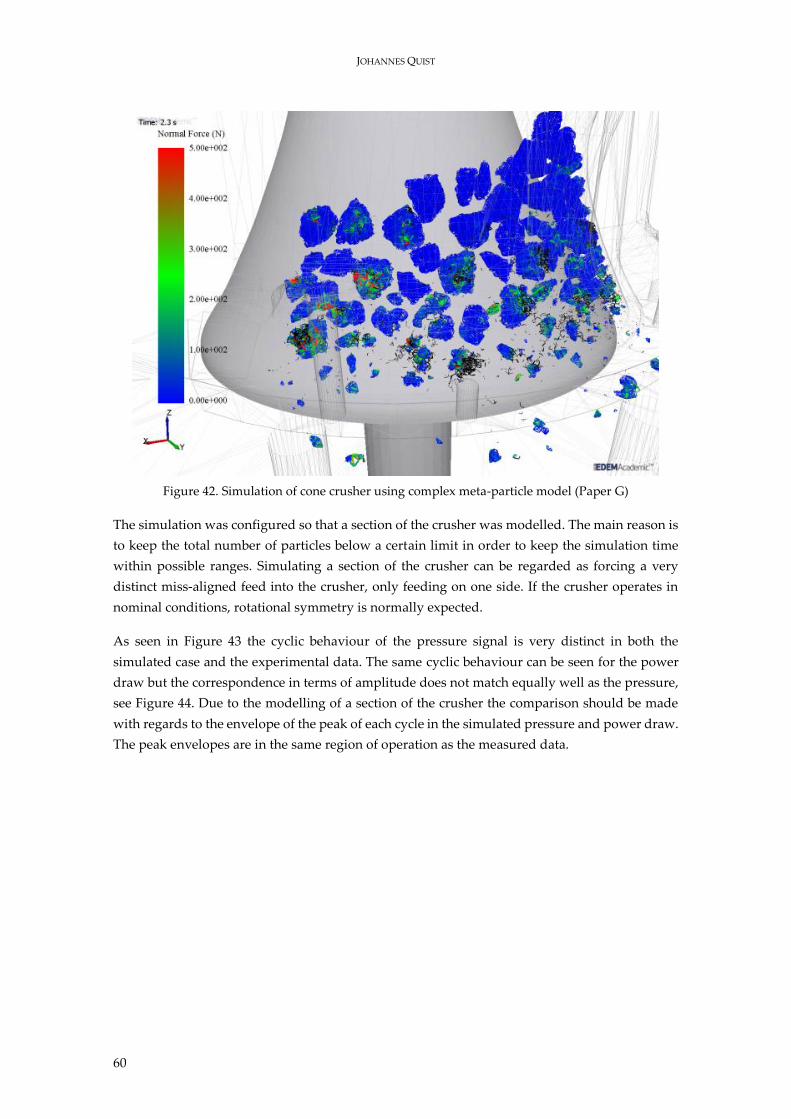
JOHANNES QUIST
60
Figure 42. Simulation of cone crusher using complex meta-particle model (Paper G)
The simulation was configured so that a section of the crusher was modelled. The main reason is
to keep the total number of particles below a certain limit in order to keep the simulation time
within possible ranges. Simulating a section of the crusher can be regarded as forcing a very
distinct miss-aligned feed into the crusher, only feeding on one side. If the crusher operates in
nominal conditions, rotational symmetry is normally expected.
As seen in Figure 43 the cyclic behaviour of the pressure signal is very distinct in both the
simulated case and the experimental data. The same cyclic behaviour can be seen for the power
draw but the correspondence in terms of amplitude does not match equally well as the pressure,
see Figure 44. Due to the modelling of a section of the crusher the comparison should be made
with regards to the envelope of the peak of each cycle in the simulated pressure and power draw.
The peak envelopes are in the same region of operation as the measured data.
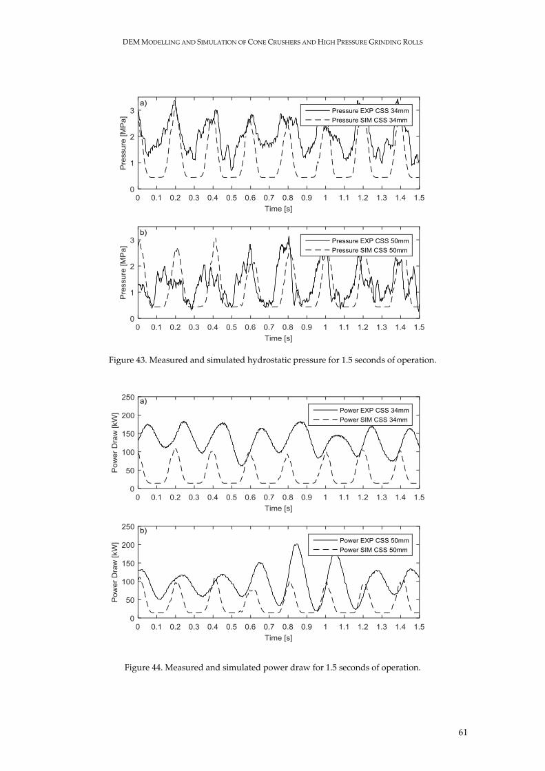
DEM MODELLING AND SIMULATION OF CONE CRUSHERS AND HIGH PRESSURE GRINDING ROLLS
61
Figure 43. Measured and simulated hydrostatic pressure for 1.5 seconds of operation.
Figure 44. Measured and simulated power draw for 1.5 seconds of operation.
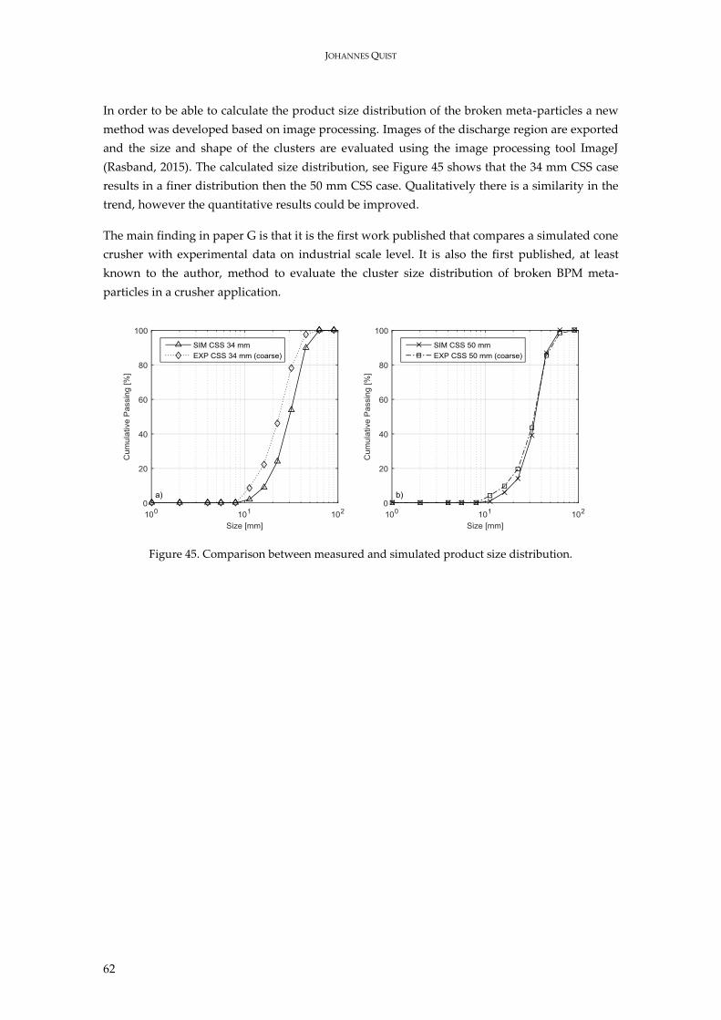
JOHANNES QUIST
62
In order to be able to calculate the product size distribution of the broken meta-particles a new
method was developed based on image processing. Images of the discharge region are exported
and the size and shape of the clusters are evaluated using the image processing tool ImageJ
(Rasband, 2015). The calculated size distribution, see Figure 45 shows that the 34 mm CSS case
results in a finer distribution then the 50 mm CSS case. Qualitatively there is a similarity in the
trend, however the quantitative results could be improved.
The main finding in paper G is that it is the first work published that compares a simulated cone
crusher with experimental data on industrial scale level. It is also the first published, at least
known to the author, method to evaluate the cluster size distribution of broken BPM meta-
particles in a crusher application.
Figure 45. Comparison between measured and simulated product size distribution.
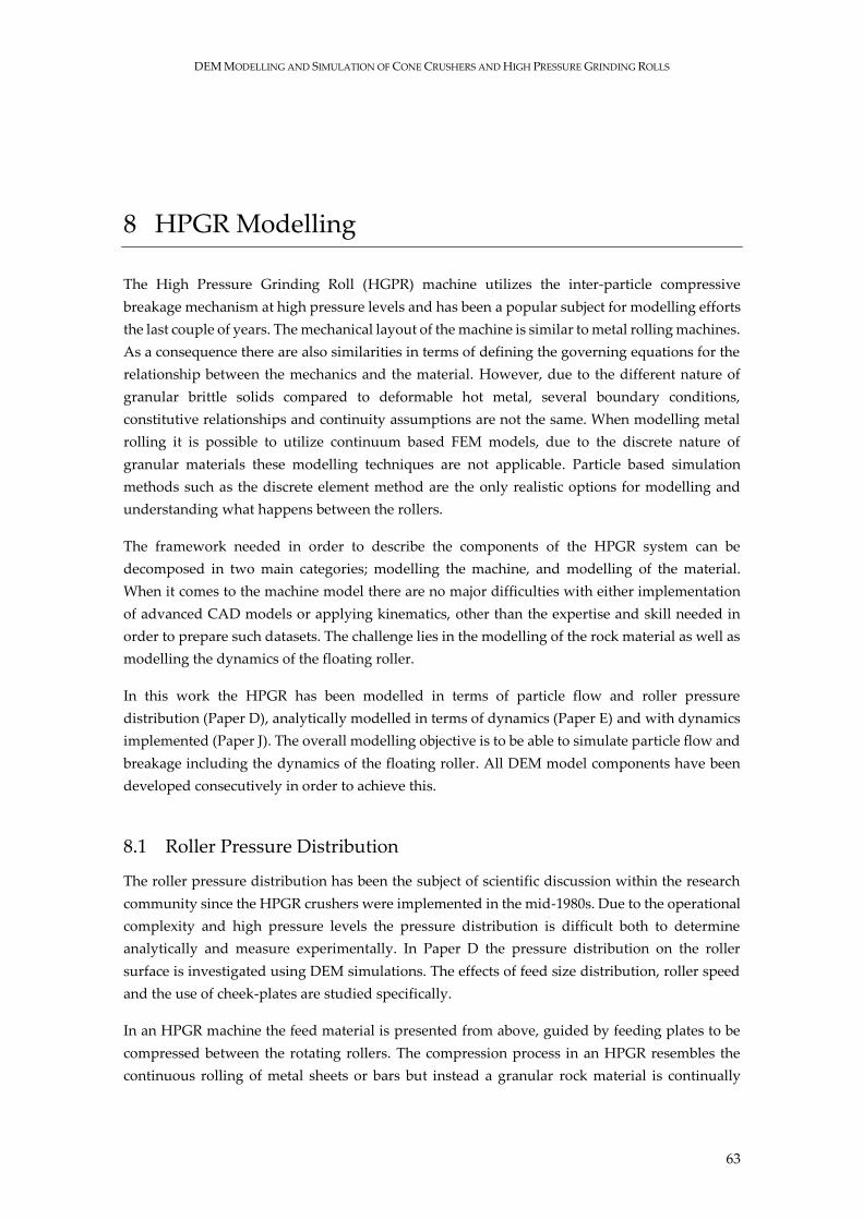
DEM MODELLING AND SIMULATION OF CONE CRUSHERS AND HIGH PRESSURE GRINDING ROLLS
63
8 HPGR Modelling
The High Pressure Grinding Roll (HGPR) machine utilizes the inter-particle compressive
breakage mechanism at high pressure levels and has been a popular subject for modelling efforts
the last couple of years. The mechanical layout of the machine is similar to metal rolling machines.
As a consequence there are also similarities in terms of defining the governing equations for the
relationship between the mechanics and the material. However, due to the different nature of
granular brittle solids compared to deformable hot metal, several boundary conditions,
constitutive relationships and continuity assumptions are not the same. When modelling metal
rolling it is possible to utilize continuum based FEM models, due to the discrete nature of
granular materials these modelling techniques are not applicable. Particle based simulation
methods such as the discrete element method are the only realistic options for modelling and
understanding what happens between the rollers.
The framework needed in order to describe the components of the HPGR system can be
decomposed in two main categories; modelling the machine, and modelling of the material.
When it comes to the machine model there are no major difficulties with either implementation
of advanced CAD models or applying kinematics, other than the expertise and skill needed in
order to prepare such datasets. The challenge lies in the modelling of the rock material as well as
modelling the dynamics of the floating roller.
In this work the HPGR has been modelled in terms of particle flow and roller pressure
distribution (Paper D), analytically modelled in terms of dynamics (Paper E) and with dynamics
implemented (Paper J). The overall modelling objective is to be able to simulate particle flow and
breakage including the dynamics of the floating roller. All DEM model components have been
developed consecutively in order to achieve this.
8.1 Roller Pressure Distribution
The roller pressure distribution has been the subject of scientific discussion within the research
community since the HPGR crushers were implemented in the mid-1980s. Due to the operational
complexity and high pressure levels the pressure distribution is difficult both to determine
analytically and measure experimentally. In Paper D the pressure distribution on the roller
surface is investigated using DEM simulations. The effects of feed size distribution, roller speed
and the use of cheek-plates are studied specifically.
In an HPGR machine the feed material is presented from above, guided by feeding plates to be
compressed between the rotating rollers. The compression process in an HPGR resembles the
continuous rolling of metal sheets or bars but instead a granular rock material is continually
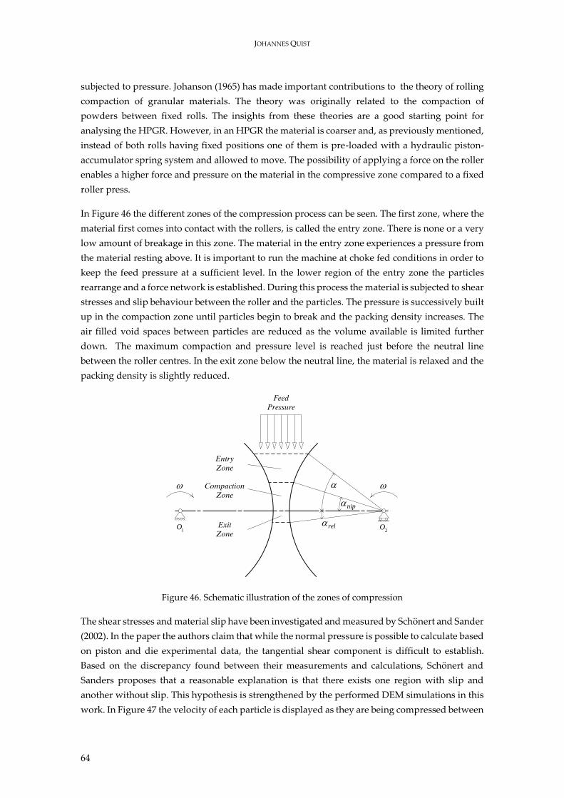
JOHANNES QUIST
64
subjected to pressure. Johanson (1965) has made important contributions to the theory of rolling
compaction of granular materials. The theory was originally related to the compaction of
powders between fixed rolls. The insights from these theories are a good starting point for
analysing the HPGR. However, in an HPGR the material is coarser and, as previously mentioned,
instead of both rolls having fixed positions one of them is pre-loaded with a hydraulic piston-
accumulator spring system and allowed to move. The possibility of applying a force on the roller
enables a higher force and pressure on the material in the compressive zone compared to a fixed
roller press.
In Figure 46 the different zones of the compression process can be seen. The first zone, where the
material first comes into contact with the rollers, is called the entry zone. There is none or a very
low amount of breakage in this zone. The material in the entry zone experiences a pressure from
the material resting above. It is important to run the machine at choke fed conditions in order to
keep the feed pressure at a sufficient level. In the lower region of the entry zone the particles
rearrange and a force network is established. During this process the material is subjected to shear
stresses and slip behaviour between the roller and the particles. The pressure is successively built
up in the compaction zone until particles begin to break and the packing density increases. The
air filled void spaces between particles are reduced as the volume available is limited further
down. The maximum compaction and pressure level is reached just before the neutral line
between the roller centres. In the exit zone below the neutral line, the material is relaxed and the
packing density is slightly reduced.
2O
1O
nip
rel
Feed Pressure
Entry Zone
Compaction Zone
Exit Zone
Figure 46. Schematic illustration of the zones of compression
The shear stresses and material slip have been investigated and measured by Schönert and Sander
(2002). In the paper the authors claim that while the normal pressure is possible to calculate based
on piston and die experimental data, the tangential shear component is difficult to establish.
Based on the discrepancy found between their measurements and calculations, Schönert and
Sanders proposes that a reasonable explanation is that there exists one region with slip and
another without slip. This hypothesis is strengthened by the performed DEM simulations in this
work. In Figure 47 the velocity of each particle is displayed as they are being compressed between
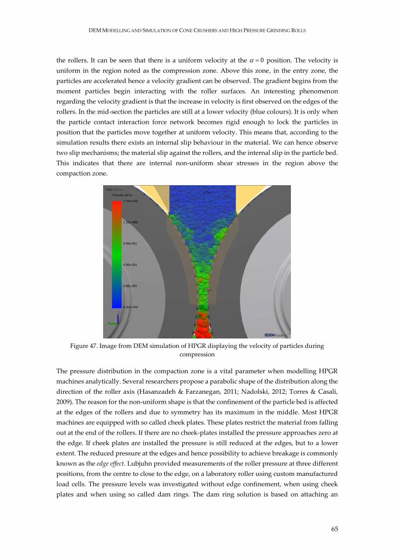
DEM MODELLING AND SIMULATION OF CONE CRUSHERS AND HIGH PRESSURE GRINDING ROLLS
65
the rollers. It can be seen that there is a uniform velocity at the 0 position. The velocity is
uniform in the region noted as the compression zone. Above this zone, in the entry zone, the
particles are accelerated hence a velocity gradient can be observed. The gradient begins from the
moment particles begin interacting with the roller surfaces. An interesting phenomenon
regarding the velocity gradient is that the increase in velocity is first observed on the edges of the
rollers. In the mid-section the particles are still at a lower velocity (blue colours). It is only when
the particle contact interaction force network becomes rigid enough to lock the particles in
position that the particles move together at uniform velocity. This means that, according to the
simulation results there exists an internal slip behaviour in the material. We can hence observe
two slip mechanisms; the material slip against the rollers, and the internal slip in the particle bed.
This indicates that there are internal non-uniform shear stresses in the region above the
compaction zone.
Figure 47. Image from DEM simulation of HPGR displaying the velocity of particles during
compression
The pressure distribution in the compaction zone is a vital parameter when modelling HPGR
machines analytically. Several researchers propose a parabolic shape of the distribution along the
direction of the roller axis (Hasanzadeh & Farzanegan, 2011; Nadolski, 2012; Torres & Casali,
2009). The reason for the non-uniform shape is that the confinement of the particle bed is affected
at the edges of the rollers and due to symmetry has its maximum in the middle. Most HPGR
machines are equipped with so called cheek plates. These plates restrict the material from falling
out at the end of the rollers. If there are no cheek-plates installed the pressure approaches zero at
the edge. If cheek plates are installed the pressure is still reduced at the edges, but to a lower
extent. The reduced pressure at the edges and hence possibility to achieve breakage is commonly
known as the edge effect. Lubjuhn provided measurements of the roller pressure at three different
positions, from the centre to close to the edge, on a laboratory roller using custom manufactured
load cells. The pressure levels was investigated without edge confinement, when using cheek
plates and when using so called dam rings. The dam ring solution is based on attaching an
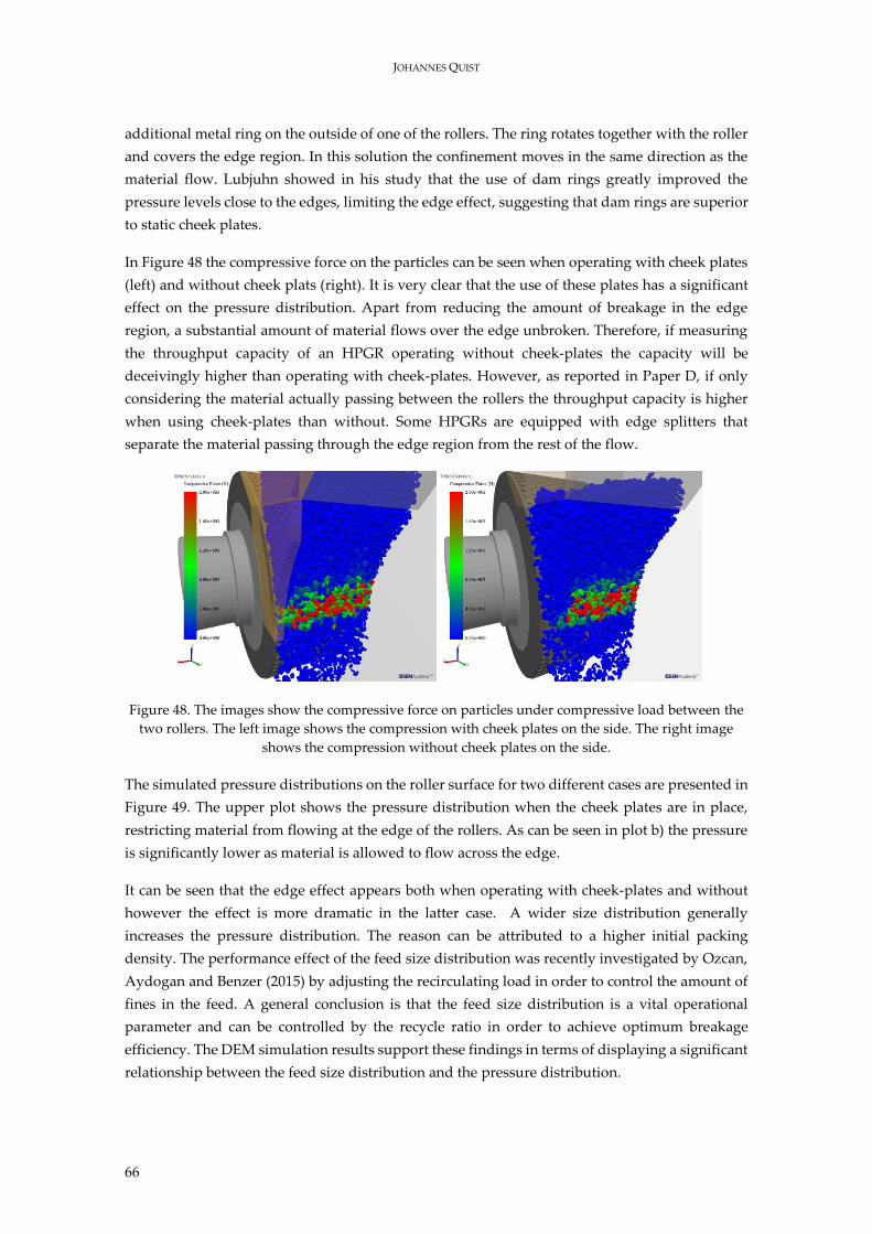
JOHANNES QUIST
66
additional metal ring on the outside of one of the rollers. The ring rotates together with the roller
and covers the edge region. In this solution the confinement moves in the same direction as the
material flow. Lubjuhn showed in his study that the use of dam rings greatly improved the
pressure levels close to the edges, limiting the edge effect, suggesting that dam rings are superior
to static cheek plates.
In Figure 48 the compressive force on the particles can be seen when operating with cheek plates
(left) and without cheek plats (right). It is very clear that the use of these plates has a significant
effect on the pressure distribution. Apart from reducing the amount of breakage in the edge
region, a substantial amount of material flows over the edge unbroken. Therefore, if measuring
the throughput capacity of an HPGR operating without cheek-plates the capacity will be
deceivingly higher than operating with cheek-plates. However, as reported in Paper D, if only
considering the material actually passing between the rollers the throughput capacity is higher
when using cheek-plates than without. Some HPGRs are equipped with edge splitters that
separate the material passing through the edge region from the rest of the flow.
Figure 48. The images show the compressive force on particles under compressive load between the
two rollers. The left image shows the compression with cheek plates on the side. The right image
shows the compression without cheek plates on the side.
The simulated pressure distributions on the roller surface for two different cases are presented in
Figure 49. The upper plot shows the pressure distribution when the cheek plates are in place,
restricting material from flowing at the edge of the rollers. As can be seen in plot b) the pressure
is significantly lower as material is allowed to flow across the edge.
It can be seen that the edge effect appears both when operating with cheek-plates and without
however the effect is more dramatic in the latter case. A wider size distribution generally
increases the pressure distribution. The reason can be attributed to a higher initial packing
density. The performance effect of the feed size distribution was recently investigated by Ozcan,
Aydogan and Benzer (2015) by adjusting the recirculating load in order to control the amount of
fines in the feed. A general conclusion is that the feed size distribution is a vital operational
parameter and can be controlled by the recycle ratio in order to achieve optimum breakage
efficiency. The DEM simulation results support these findings in terms of displaying a significant
relationship between the feed size distribution and the pressure distribution.
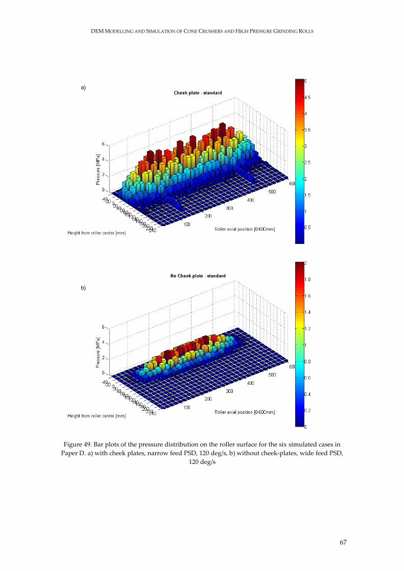
DEM MODELLING AND SIMULATION OF CONE CRUSHERS AND HIGH PRESSURE GRINDING ROLLS
67
Figure 49. Bar plots of the pressure distribution on the roller surface for the six simulated cases in
Paper D. a) with cheek plates, narrow feed PSD, 120 deg/s, b) without cheek-plates, wide feed PSD,
120 deg/s
a)
b)
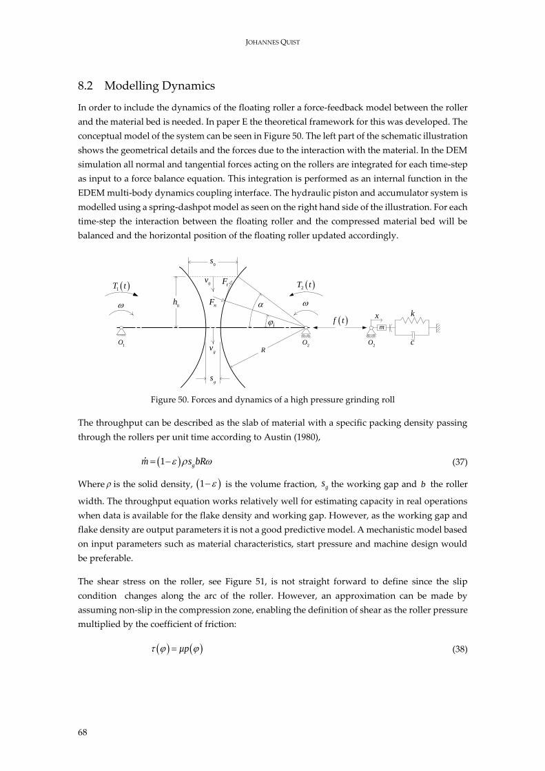
JOHANNES QUIST
68
8.2 Modelling Dynamics
In order to include the dynamics of the floating roller a force-feedback model between the roller
and the material bed is needed. In paper E the theoretical framework for this was developed. The
conceptual model of the system can be seen in Figure 50. The left part of the schematic illustration
shows the geometrical details and the forces due to the interaction with the material. In the DEM
simulation all normal and tangential forces acting on the rollers are integrated for each time-step
as input to a force balance equation. This integration is performed as an internal function in the
EDEM multi-body dynamics coupling interface. The hydraulic piston and accumulator system is
modelled using a spring-dashpot model as seen on the right hand side of the illustration. For each
time-step the interaction between the floating roller and the compressed material bed will be
balanced and the horizontal position of the floating roller updated accordingly.
Figure 50. Forces and dynamics of a high pressure grinding roll
The throughput can be described as the slab of material with a specific packing density passing
through the rollers per unit time according to Austin (1980),
1 gm s bR (37)
Where is the solid density, 1 is the volume fraction, gs the working gap and b the roller
width. The throughput equation works relatively well for estimating capacity in real operations
when data is available for the flake density and working gap. However, as the working gap and
flake density are output parameters it is not a good predictive model. A mechanistic model based
on input parameters such as material characteristics, start pressure and machine design would
be preferable.
The shear stress on the roller, see Figure 51, is not straight forward to define since the slip
condition changes along the arc of the roller. However, an approximation can be made by
assuming non-slip in the compression zone, enabling the definition of shear as the roller pressure
multiplied by the coefficient of friction:
µp (38)
gv
gs
0s
i
0v
0h
R
k
c
x
m
2O
2O
1O
1T t 2T t
f t
tF
nF
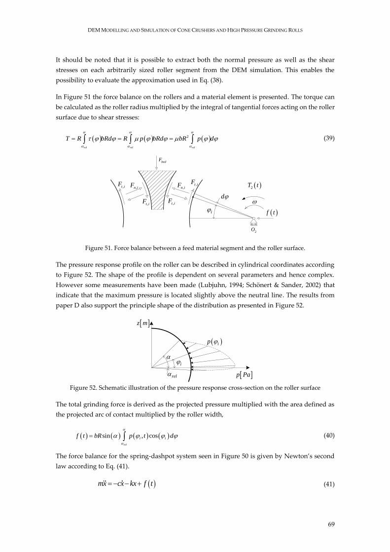
DEM MODELLING AND SIMULATION OF CONE CRUSHERS AND HIGH PRESSURE GRINDING ROLLS
69
It should be noted that it is possible to extract both the normal pressure as well as the shear
stresses on each arbitrarily sized roller segment from the DEM simulation. This enables the
possibility to evaluate the approximation used in Eq. (38).
In Figure 51 the force balance on the rollers and a material element is presented. The torque can
be calculated as the roller radius multiplied by the integral of tangential forces acting on the roller
surface due to shear stresses:
2
rel rel rel
T R bRd R p bRd bR p d
(39)
Figure 51. Force balance between a feed material segment and the roller surface.
The pressure response profile on the roller can be described in cylindrical coordinates according
to Figure 52. The shape of the profile is dependent on several parameters and hence complex.
However some measurements have been made (Lubjuhn, 1994; Schönert & Sander, 2002) that
indicate that the maximum pressure is located slightly above the neutral line. The results from
paper D also support the principle shape of the distribution as presented in Figure 52.
Figure 52. Schematic illustration of the pressure response cross-section on the roller surface
The total grinding force is derived as the projected pressure multiplied with the area defined as
the projected arc of contact multiplied by the roller width,
sin , cos
rel
i if t bR p t d
(40)
The force balance for the spring-dashpot system seen in Figure 50 is given by Newton’s second
law according to Eq. (41).
mx cx kx f t (41)
bedF
i
2O
d
f t
2T t,n iF
,t iF
,n iF ,t iF
,t iF
,t iF
i
ip
rel
z m
p Pa
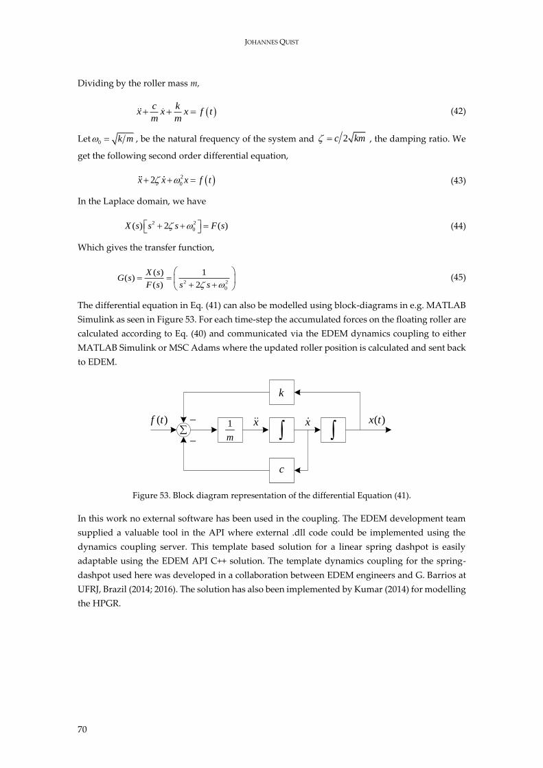
JOHANNES QUIST
70
Dividing by the roller mass m,
c k
x x x f tm m
(42)
Let 0 k m , be the natural frequency of the system and 2c km , the damping ratio. We
get the following second order differential equation,
2
02x x x f t (43)
In the Laplace domain, we have
2 2
0( ) 2 ( )X s s s F s (44)
Which gives the transfer function,
2 2
0
( ) 1( )
( ) 2
X sG s
F s s s
(45)
The differential equation in Eq. (41) can also be modelled using block-diagrams in e.g. MATLAB
Simulink as seen in Figure 53. For each time-step the accumulated forces on the floating roller are
calculated according to Eq. (40) and communicated via the EDEM dynamics coupling to either
MATLAB Simulink or MSC Adams where the updated roller position is calculated and sent back
to EDEM.
Figure 53. Block diagram representation of the differential Equation (41).
In this work no external software has been used in the coupling. The EDEM development team
supplied a valuable tool in the API where external .dll code could be implemented using the
dynamics coupling server. This template based solution for a linear spring dashpot is easily
adaptable using the EDEM API C++ solution. The template dynamics coupling for the spring-
dashpot used here was developed in a collaboration between EDEM engineers and G. Barrios at
UFRJ, Brazil (2014; 2016). The solution has also been implemented by Kumar (2014) for modelling
the HPGR.
1
m
k
cc
( )f t x x ( )x t
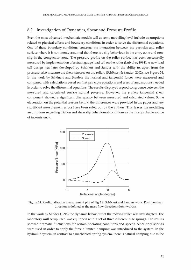
DEM MODELLING AND SIMULATION OF CONE CRUSHERS AND HIGH PRESSURE GRINDING ROLLS
71
8.3 Investigation of Dynamics, Shear and Pressure Profile
Even the most advanced mechanistic models will at some modelling level include assumptions
related to physical effects and boundary conditions in order to solve the differential equations.
One of these boundary conditions concerns the interaction between the particles and roller
surface where it is commonly assumed that there is a slip behaviour in the entry zone and non-
slip in the compaction zone. The pressure profile on the roller surface has been successfully
measured by implementation of a strain gauge load cell on the roller (Lubjuhn, 1994). A new load
cell design was later developed by Schönert and Sander with the ability to, apart from the
pressure, also measure the shear stresses on the rollers (Schönert & Sander, 2002), see Figure 54.
In the work by Schönert and Sanders the normal and tangential forces were measured and
compared with calculations based on first principle equations and a set of assumptions needed
in order to solve the differential equations. The results displayed a good congruence between the
measured and calculated surface normal pressure. However, the surface tangential shear
component showed a significant discrepancy between measured and calculated values. Some
elaboration on the potential reasons behind the differences were provided in the paper and any
significant measurement errors have been ruled out by the authors. This leaves the modelling
assumptions regarding friction and shear slip behavioural conditions as the most probable source
of inconsistency.
Figure 54. Re-digitalization measurement plot of Fig 3 in Schönert and Sanders work. Positive shear
direction is defined as the mass flow direction (downwards).
In the work by Sander (1998) the dynamic behaviour of the moving roller was investigated. The
laboratory mill setup used was equipped with a set of three different disc springs. The results
showed dramatic fluctuations for certain operating conditions and speeds. Since only springs
were used in order to apply the force a limited damping was introduced to the system. In the
hydraulic system, in contrast to a mechanical spring system, there is natural damping due to the
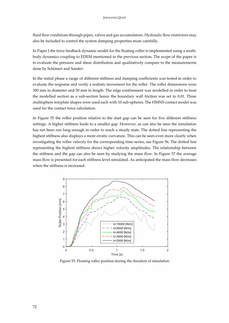
JOHANNES QUIST
72
fluid flow conditions through pipes, valves and gas accumulators. Hydraulic flow restrictors may
also be included to control the system damping properties more carefully.
In Paper J the force feedback dynamic model for the floating roller is implemented using a multi-
body dynamics coupling to EDEM mentioned in the previous section. The scope of the paper is
to evaluate the pressure and shear distribution and qualitatively compare to the measurements
done by Schönert and Sander.
In the initial phase a range of different stiffness and damping coefficients was tested in order to
evaluate the response and verify a realistic movement for the roller. The roller dimensions were
300 mm in diameter and 50 mm in length. The edge confinement was modelled in order to treat
the modelled section as a sub-section hence the boundary wall friction was set to 0.01. Three
multisphere template shapes were used each with 10 sub-spheres. The HMNS contact model was
used for the contact force calculation.
In Figure 55 the roller position relative to the start gap can be seen for five different stiffness
settings. A higher stiffness leads to a smaller gap. However, as can also be seen the simulation
has not been run long enough in order to reach a steady state. The dotted line representing the
highest stiffness also displays a more erratic curvature. This can be seen even more clearly when
investigating the roller velocity for the corresponding time-series, see Figure 56. The dotted line
representing the highest stiffness shows higher velocity amplitudes. The relationship between
the stiffness and the gap can also be seen by studying the mass flow. In Figure 57 the average
mass flow is presented for each stiffness level simulated. As anticipated the mass flow decreases
when the stiffness is increased.
Figure 55. Floating roller position during the duration of simulation
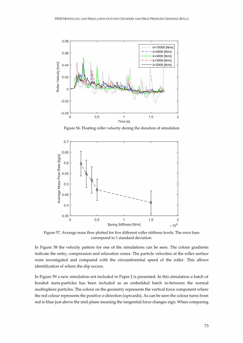
DEM MODELLING AND SIMULATION OF CONE CRUSHERS AND HIGH PRESSURE GRINDING ROLLS
73
Figure 56. Floating roller velocity during the duration of simulation
Figure 57. Average mass flow plotted for five different roller stiffness levels. The error bars
correspond to 1 standard deviation.
In Figure 58 the velocity pattern for one of the simulations can be seen. The colour gradients
indicate the entry, compression and relaxation zones. The particle velocities at the roller surface
were investigated and compared with the circumferential speed of the roller. This allows
identification of where the slip occurs.
In Figure 59 a new simulation not included in Paper J is presented. In this simulation a batch of
bonded meta-particles has been included as an embedded batch in-between the normal
multisphere particles. The colour on the geometry represents the vertical force component where
the red colour represents the positive z-direction (upwards). As can be seen the colour turns from
red to blue just above the mid-plane meaning the tangential force changes sign. When comparing
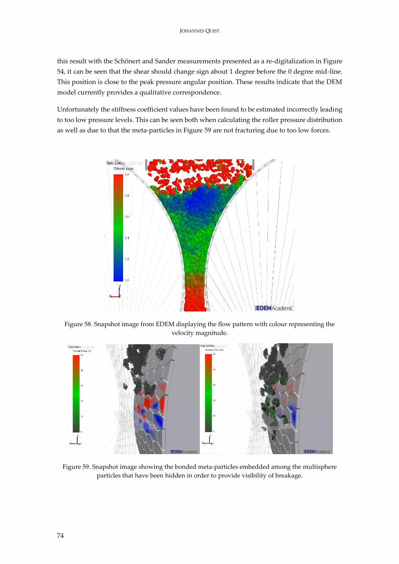
JOHANNES QUIST
74
this result with the Schönert and Sander measurements presented as a re-digitalization in Figure
54, it can be seen that the shear should change sign about 1 degree before the 0 degree mid-line.
This position is close to the peak pressure angular position. These results indicate that the DEM
model currently provides a qualitative correspondence.
Unfortunately the stiffness coefficient values have been found to be estimated incorrectly leading
to too low pressure levels. This can be seen both when calculating the roller pressure distribution
as well as due to that the meta-particles in Figure 59 are not fracturing due to too low forces.
Figure 58. Snapshot image from EDEM displaying the flow pattern with colour representing the
velocity magnitude.
Figure 59. Snapshot image showing the bonded meta-particles embedded among the multisphere
particles that have been hidden in order to provide visibility of breakage.
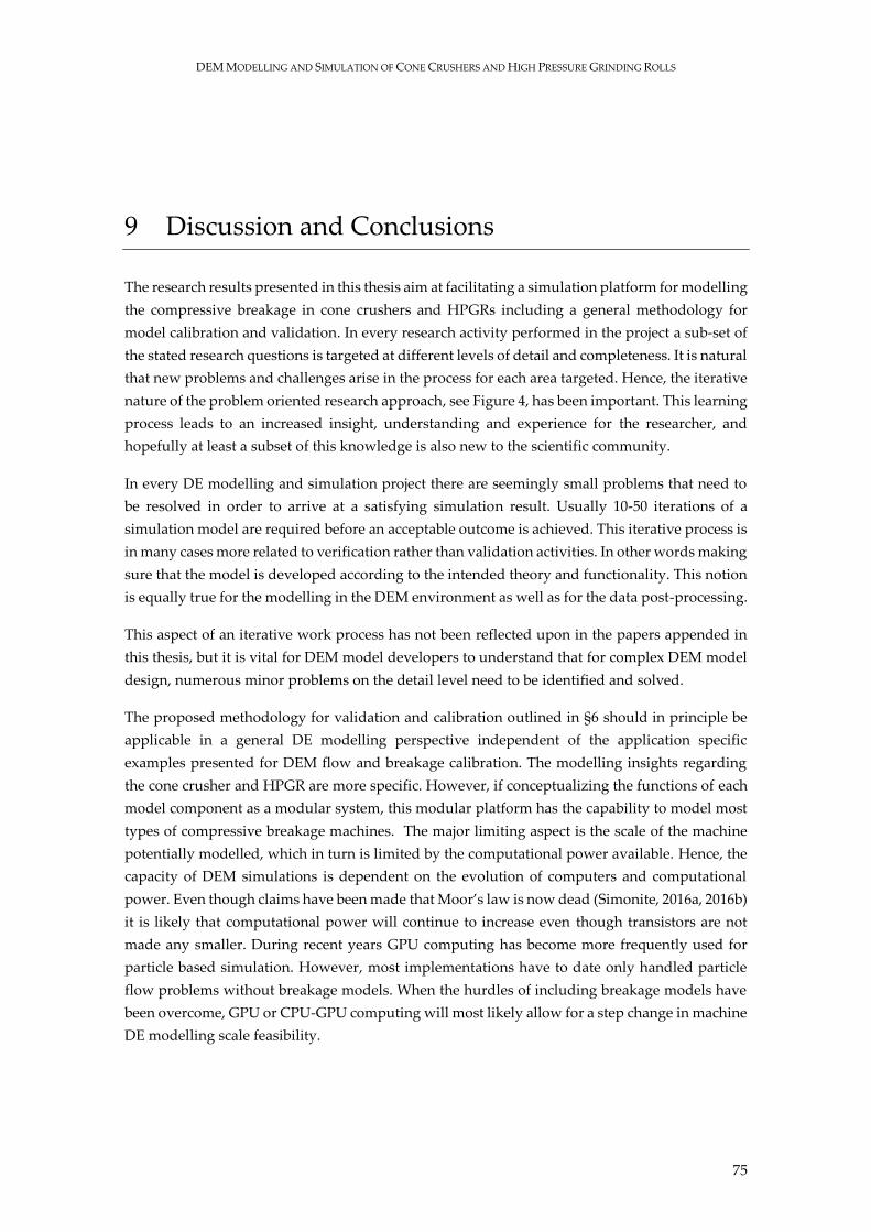
DEM MODELLING AND SIMULATION OF CONE CRUSHERS AND HIGH PRESSURE GRINDING ROLLS
75
9 Discussion and Conclusions
The research results presented in this thesis aim at facilitating a simulation platform for modelling
the compressive breakage in cone crushers and HPGRs including a general methodology for
model calibration and validation. In every research activity performed in the project a sub-set of
the stated research questions is targeted at different levels of detail and completeness. It is natural
that new problems and challenges arise in the process for each area targeted. Hence, the iterative
nature of the problem oriented research approach, see Figure 4, has been important. This learning
process leads to an increased insight, understanding and experience for the researcher, and
hopefully at least a subset of this knowledge is also new to the scientific community.
In every DE modelling and simulation project there are seemingly small problems that need to
be resolved in order to arrive at a satisfying simulation result. Usually 10-50 iterations of a
simulation model are required before an acceptable outcome is achieved. This iterative process is
in many cases more related to verification rather than validation activities. In other words making
sure that the model is developed according to the intended theory and functionality. This notion
is equally true for the modelling in the DEM environment as well as for the data post-processing.
This aspect of an iterative work process has not been reflected upon in the papers appended in
this thesis, but it is vital for DEM model developers to understand that for complex DEM model
design, numerous minor problems on the detail level need to be identified and solved.
The proposed methodology for validation and calibration outlined in §6 should in principle be
applicable in a general DE modelling perspective independent of the application specific
examples presented for DEM flow and breakage calibration. The modelling insights regarding
the cone crusher and HPGR are more specific. However, if conceptualizing the functions of each
model component as a modular system, this modular platform has the capability to model most
types of compressive breakage machines. The major limiting aspect is the scale of the machine
potentially modelled, which in turn is limited by the computational power available. Hence, the
capacity of DEM simulations is dependent on the evolution of computers and computational
power. Even though claims have been made that Moor’s law is now dead (Simonite, 2016a, 2016b)
it is likely that computational power will continue to increase even though transistors are not
made any smaller. During recent years GPU computing has become more frequently used for
particle based simulation. However, most implementations have to date only handled particle
flow problems without breakage models. When the hurdles of including breakage models have
been overcome, GPU or CPU-GPU computing will most likely allow for a step change in machine
DE modelling scale feasibility.
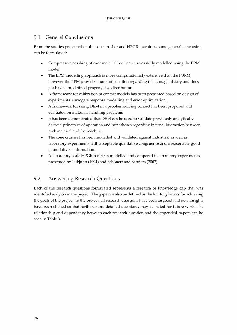
JOHANNES QUIST
76
9.1 General Conclusions
From the studies presented on the cone crusher and HPGR machines, some general conclusions
can be formulated:
Compressive crushing of rock material has been successfully modelled using the BPM
model
The BPM modelling approach is more computationally extensive than the PBRM,
however the BPM provides more information regarding the damage history and does
not have a predefined progeny size distribution.
A framework for calibration of contact models has been presented based on design of
experiments, surrogate response modelling and error optimization.
A framework for using DEM in a problem solving context has been proposed and
evaluated on materials handling problems
It has been demonstrated that DEM can be used to validate previously analytically
derived principles of operation and hypotheses regarding internal interaction between
rock material and the machine
The cone crusher has been modelled and validated against industrial as well as
laboratory experiments with acceptable qualitative congruence and a reasonably good
quantitative conformation.
A laboratory scale HPGR has been modelled and compared to laboratory experiments
presented by Lubjuhn (1994) and Schönert and Sanders (2002).
9.2 Answering Research Questions
Each of the research questions formulated represents a research or knowledge gap that was
identified early on in the project. The gaps can also be defined as the limiting factors for achieving
the goals of the project. In the project, all research questions have been targeted and new insights
have been elicited so that further, more detailed questions, may be stated for future work. The
relationship and dependency between each research question and the appended papers can be
seen in Table 3.
DEM MODELLING AND SIMULATION OF CONE CRUSHERS AND HIGH PRESSURE GRINDING ROLLS
77
Table 3. The dependency matrix displays the relationship between research questions and papers,
with the size of the circle (three levels) corresponding to a subjectively judged level of focus.
Papers
Research Question A B C D E F G H I J
RQ.1 Operational understanding
RQ.2 Design process methodology
RQ.3 Rock breakage modelling
RQ.4 Product particle size
distribution
RQ.5 Flow calibration
RQ.6 Breakage calibration
RQ.7 Machine geometry modelling
RQ.8 Machine dynamics
RQ.9 Power draw and pressure
RQ.10 Simulation validation
9.3 Scientific Contribution
The results presented can either be attributed to strengthening previous findings by others,
contradicting findings by others, or being novel findings and models. In the section below a list
of detailed findings is presented for each research question respectively.
RQ.1 How should DEM be used to understand and diagnose operating equipment in comminution
processes?
A new framework for the work flow of problem solving and concept development
using DEM has been proposed.
The framework has successfully been demonstrated for a cone crusher feeding
materials handling problem
The framework has successfully been demonstrated for laboratory cone crusher liner
design development
RQ.2 How should DEM be used as a design evaluation tool in a product development context?
The use of DEM as a concept evaluation tool has been demonstrated using the
proposed DEM design process.
For the first simulation in step i, a high level of fidelity should be applied in terms of
geometry and particle material model
Lower fidelity simulation models, balanced against the predictive accuracy, may be
used in order to quickly evaluate the principle of different conceptual solutions
JOHANNES QUIST
78
RQ.3 How should rock breakage in compressive breakage machines be modelled in order to balance
validity and computational economy?
A new bonded particle model utilizing a bimodal size distribution for fraction
particles has been developed. It was found that a bimodal distribution offers the best
packing behaviour and minimum number of particles in each meta-particle while
maintaining sufficient quality of the breakage behaviour. The bimodal distribution
affects bond beam strength distribution enabling a heterogeneous strength
distribution within the body of the meta-particle.
A novel method for creating realistic irregular rock particle shape of meta-particles
has been developed based on 3D-scanned rock particles.
RQ.4 What is a suitable method for calculating the particle size distribution of bonded particle model?
A new method, based on image processing, for calculating the product size
distribution of progeny meta-particle clusters has been developed and compared
with industrial scale data.
RQ.5 How should DEM material models be calibrated with regards to particle flow?
A new calibration and validation framework has been proposed and demonstrated.
The framework is based on optimization of the pragmatic congruence tolerance
between the experimental and the simulation based surrogate model.
The concept of multi objective optimization has been applied to the calibration
process of contact model parameters for multiple flow regimes.
A new device for calibration of DEM contact model parameters has been designed
and demonstrated.
It has been demonstrated that contact model parameter calibration needs to be
conducted using multiple flow regimes.
A new method for capturing real single particle flow within a bulk flow using
marker particles and motion capture technique has been developed.
A new method for calculating the repose angle from simulated pile formation by
fitting a sigmoid function to the free surface layer particle positions has been
developed.
It has been demonstrated that the dynamic repose angle is dependent on the flow
velocity of the bulk material prior to bed formation.
RQ.6 How should DEM material models be calibrated with regards to particle breakage?
A calibration procedure for BPM models using Brazilian tensile strength test has
been developed.
A framework for breakage model calibration has been proposed based on surrogate-
based optimization
It has been demonstrated that the model accuracy has a trade-off pareto relationship
to the computational load
DEM MODELLING AND SIMULATION OF CONE CRUSHERS AND HIGH PRESSURE GRINDING ROLLS
79
RQ.7 How should machine geometry be modelled in DEM?
3D-scanning point cloud data has been used for modelling primary gyratory
crushers. This is the first time reported in literature that point clouds are used for
DEM simulations of crushers.
3D scanning point cloud data has been used for modelling machine geometry of
industrial scale cone crusher liners in order to match the actual worn state of the
machine.
RQ.8 How should machine dynamics be integrated with DEM?
The framework for the dynamic model of the HPGR has been developed and
implemented.
The dynamics of the HPGR rollers have been analysed for different stiffness and
damping characteristics
RQ.9 How should the estimation of forces, pressure and power draw be conducted?
The power draw and pressure have been calculated and compared to an industrial
scale cone crusher
A method for calculating the pressure distribution on the roller surface based on
DEM simulation data has been developed.
RQ.10 How should DEM simulations be validated?
The V-model for DEM calibration and validation has been proposed
So called face validity has been demonstrated when comparing DEM simulation
results with findings from analytical modelling (C.M. Evertsson, 2000) (using first
principle mechanics) regarding choke level positions, breakage mode and particle
squeezing behaviour in the crushing chamber.
A laboratory scale validation case of a cone crusher operated at high eccentric speed
has been demonstrated
An industrial scale validation case of a secondary stage cone crusher has been
demonstrated.
9.4 Vision for further development
The utopia of discrete element breakage modelling would be to simulate a machine in full
operation with a material model in which the real rock grain size distribution and texture is
represented. Let’s exemplify by considering a small machine where 1 litre of material is subjected
to a mechanical breakage environment. If the mean grain size of a relatively coarse rock texture
would be 1 mm and we approximate the shape of each grain by a cube. Then the corresponding
number of particles or voxels needed for one litre of rock would be 1 million. The current state of
the art DEM codes are capable of simulating up to 5-15 million particles. However, the benchmark
simulations then usually referred to are flow simulations and do not consider the computational
JOHANNES QUIST
80
load increase due to modelling of any bonding interactions. It is hence currently not a feasible
approach forward to model 10-100 litres of material in full resolution at once.
What can be done however, is to model each meta-particle rock with a larger grain size
distribution than the actual, which is what is being done in this work. Through the calibration
process the bonds between the fraction particles may still be defined in order to achieve a useful
breakage response. While useful for evaluating machine design, it may not be useful for rock
mechanics research purposes.
A novel alternative solution (future work) to the PBRM and BPM implementation would be to
combine them. Before proceeding to explain this solution, a brief repetition on how the BPM is
currently created may be needed. In the current BPM implementation the fraction particles are
included in the simulation at a pre-defined time. At this time step a set of dummy particles is
replaced by the cluster of fraction particles forming the meta-particle. This replacement action is
in fact very similar to the breakage replacement algorithm implemented for the PBRM model.
The difference is that in the BPM case the replacement is triggered at a pre-defined time, and in
the PBRM case it is triggered by a loading condition.
Instead of triggering the replacement action either by load or time, the replacement could take
place based on position. Hence, instead of creating all BPM meta-particles in a batch, they would
stay as inexpensive non-breakage particles, until they enter a ‘risk of damage domain’. The
damage domain would correspond to the crushing chamber in a cone crusher and the
compression zone in the HPGR.
This model has not yet been implemented in this work but would require the following changes:
The replacement to be initiated based on a spatial domain constraint
Improve the replacement function to allow for the use of multi-spheres as dummy
particles
Implement orientation compliance in the replacement function in order to align the
multisphere domain and the meta-particle.
The BPM model needs to be re-formulated so that the bonding action is activated at each
continuous replacement event. However, only the most recently fraction cluster particles
are allowed to bond. Otherwise there is a risk of bonding chunks of meta-particles
together or re-bonding already broken clusters.
This approach would allow for a high resolution BPM or TEM modelling approach by taking
advantage of the engineers/modellers knowledge regarding where the breakage will take place.
Finally, the results presented in this thesis demonstrate that fundamental novel understanding
regarding comminution equipment can be achieved using DEM. For research and development
departments operating in the mining and aggregate industry that seriously begin using particle
based simulation methods, there will be no way back.
DEM MODELLING AND SIMULATION OF CONE CRUSHERS AND HIGH PRESSURE GRINDING ROLLS
81
10 References
Antonyuk, S., Khanal, M., Tomas, J., Heinrich, S., Mörl, L. (2006). Impact breakage of spherical granules:
Experimental study and DEM simulation. Chemical Engineering and Processing, 45, 838-856.
ASME. (2006). Guide for Verification and Validation in Computational Solid Mechanics (Vol. V V 10 - 2006):
THE AMERICAN SOCIETY OF MECHANICAL ENGINEERS.
ASTM. (2008). Standard Test Method for Splitting Tensile Strength of Intact Rock Core Specimens (Vol.
D3967 - 08). United States: ASTM International.
Austin, L. G., Van Orden, D. R., & Pérez, J. W. (1980). A preliminary analysis of smooth roll crushers.
International Journal of Mineral Processing, 6(4), 321-336. doi:10.1016/0301-7516(80)90028-9
Barker, P. E., & Watson, H. K. (1969). Calibrating the simulation model of the IBM system/360 time sharing system.
Paper presented at the Proceedings of the third conference on Applications of simulation, Los
Angeles, California, USA.
Barrios, G., Tavares, M., Pérez-Prim, J. (2014). High pressure grinding rolls simulation using the discrete element
method dynamic coupling interface. Paper presented at the XXVII International Mineral Processing
Congress, Santiago, Chile.
Barrios, G. K. P., de Carvalho, R. M., Kwade, A., & Tavares, L. M. (2013). Contact parameter estimation for
DEM simulation of iron ore pellet handling. Powder Technology, 248(0), 84-93.
doi:http://dx.doi.org/10.1016/j.powtec.2013.01.063
Barrios, G. K. P., & Tavares, L. M. (2016). A preliminary model of high pressure roll grinding using the
discrete element method and multi-body dynamics coupling. International Journal of Mineral
Processing, 156, 32-42. doi:http://dx.doi.org/10.1016/j.minpro.2016.06.009
Behraftar, S., Galindo Torres, S. A., Scheuermann, A., Williams, D. J., Marques, E. A. G., & Janjani
Avarzaman, H. (2017). A calibration methodology to obtain material parameters for the
representation of fracture mechanics based on discrete element simulations. Computers and
Geotechnics, 81, 274-283. doi:http://dx.doi.org/10.1016/j.compgeo.2016.08.029
Benzer, H., Aydogan, N. A., & Dündar, H. (2011). Investigation of the breakage of hard and soft components
under high compression: HPGR application. Minerals Engineering, 24(3–4), 303-307.
doi:10.1016/j.mineng.2010.09.012
Box, G. E. P., J. Stuart Hunter, and William Gordon Hunter. (2005). Statistics for Experimenters: Design,
Innovation, and Discovery (Vol. 2nd ed). Hoboken, N.J: Wiley-Interscience.
Brouwers, H. J. H. (2006). Particle-size distribution and packing fraction of geometric random packings.
PHYSICAL REVIEW, 74. doi:10.1103/PhysRevE.74.031309
Brown, N., Chen, J.-F., & Ooi, J. (2014). A bond model for DEM simulation of cementitious materials and
deformable structures. Granular Matter, 16(3), 299-311. doi:10.1007/s10035-014-0494-4
Cho, N., Martin, C. D., & Sego, D. C. (2007). A clumped particle model for rock. International Journal of Rock
Mechanics and Mining Sciences, 44(7), 997-1010. doi:http://dx.doi.org/10.1016/j.ijrmms.2007.02.002
Cleary, P. W. (2001). Recent advances in dem modelling of tumbling mills. Minerals Engineering, 14(10), 1295-
1319. doi:http://dx.doi.org/10.1016/S0892-6875(01)00145-5
JOHANNES QUIST
82
Cleary, P. W., & Sinnott, M. D. (2015). Simulation of particle flows and breakage in crushers using DEM:
Part 1 – Compression crushers. Minerals Engineering, 74(0), 178-197.
doi:http://dx.doi.org/10.1016/j.mineng.2014.10.021
Cleary, P. W., Sinnott, M. D., Morrison, R. D., Cummins, S., & Delaney, G. W. (2017). Analysis of cone crusher
performance with changes in material properties and operating conditions using DEM. Minerals
Engineering, 100, 49-70. doi:http://dx.doi.org/10.1016/j.mineng.2016.10.005
Coetzee, C. J. (2017). Review: Calibration of the discrete element method. Powder Technology, 310, 104-142.
doi:http://dx.doi.org/10.1016/j.powtec.2017.01.015
Coetzee, C. J., Els, D.N.J. (2009). Calibration of discrete element parameters and the modelling of silo
discharge and bucket filling. Computers and electronics in agriculture, 65, 198-212.
Coetzee, C. J., & Nel, R. G. (2014). Calibration of discrete element properties and the modelling of packed
rock beds. Powder Technology, 264(0), 332-342. doi:http://dx.doi.org/10.1016/j.powtec.2014.05.063
Combarros, M., Feise, H. J., Zetzener, H., & Kwade, A. (2014). Segregation of particulate solids: Experiments
and DEM simulations. Particuology, 12(0), 25-32. doi:http://dx.doi.org/10.1016/j.partic.2013.04.005
Cundall, P. A. (1971). A computer model for large scale movements of blocky rock systems. Paper presented at the
Proc. Symp. ISPM., Nancy, France.
Cundall, P. A. (1988). Formulation of a three-dimensional distinct element mode – part I: a scheme to detect
and represent contacts in a system composed of many polyhedral blocks. International Journal of
Rock Mechanics and Mining Sciences & Geomechanics Abstracts, 25(3), 107-116.
Cundall, P. A., & Strack, O. D. L. (1979). A discrete numerical model for granular assemblies. Geotechnique,
29(1), 47-65.
Cundall, P. A., Strack, O.D. (1979). A discrete numerical model for granular assemblies. Geotechnique, 29(1),
47-65.
Daniel, M. J., & Morrell, S. (2004). HPGR model verification and scale-up. Minerals Engineering, 17(11–12),
1149-1161. doi:10.1016/j.mineng.2004.05.016
Das, R., & Cleary, P. W. (2010). Effect of rock shapes on brittle fracture using Smoothed Particle
Hydrodynamics. Theoretical and Applied Fracture Mechanics, 53(1), 47-60.
doi:http://dx.doi.org/10.1016/j.tafmec.2009.12.004
Delaney, G. W., Cleary, P. W., Sinnott, M. D., & Morrison, R. D. (2010). Novel application of DEM to modelling
comminution processes. Paper presented at the 9th World Congress on computational Mechanics,
Sydney, Australia.
Delaney, G. W., Morrison, R. D., Sinnott, M. D., Cummins, S., & Cleary, P. W. (2015). DEM modelling of
non-spherical particle breakage and flow in an industrial scale cone crusher. Minerals Engineering,
74(0), 112-122. doi:http://dx.doi.org/10.1016/j.mineng.2015.01.013
Djordjevic, N., Shi, F. N., & Morrison, R. D. (2003). Applying discrete element modelling to vertical and
horizontal shaft impact crushers. Minerals Engineering, 16(10), 983-991.
doi:http://dx.doi.org/10.1016/j.mineng.2003.08.007
Eckhardt, R. (1987). Stan Ulam, John von Neumann, and the Monte Carlo Method. Los Alamos Science Special
Issue(15).
Ergenzinger, C., Seifried, R., & Eberhard, P. (2012). A discrete element model predicting the strength of
ballast stones. Computers & Structures, 108–109(0), 3-13.
doi:http://dx.doi.org/10.1016/j.compstruc.2012.02.006
Ergenzinger, C., Seifried, R., Eberhard P. (2011). A discrete element model to describe failure of strong rock
in uniaxial compression. Granular Matter, 13(4), 341-364. doi:10.1007/s10035-010-0230-7
Euler, L. (1768). Institutiones calculi integralis. Petropoli: Impenfis Academiae Imperialis Scientiarum.
DEM MODELLING AND SIMULATION OF CONE CRUSHERS AND HIGH PRESSURE GRINDING ROLLS
83
Evertsson, C. M. (1999). Modelling of flow in cone crushers. Minerals Engineering, 12(12), 1479-1499.
Evertsson, C. M. (2000). Cone Crusher Performance. (PhD thesis), Chalmers University of Technology, Sweden.
Fairhurst, C. (1964). On the validity of the ‘Brazilian’ test for brittle materials. International Journal of Rock
Mechanics and Mining Sciences & Geomechanics Abstracts, 1(4), 535-546.
doi:http://dx.doi.org/10.1016/0148-9062(64)90060-9
Favier, J., Curry, D., LaRoche R. (2010). Calibration of DEM material models to approximate bulk particle
characteristics. Paper presented at the 6th World Congress on Particle Technology, Nuremberg,
Germany.
Forrester, A. I. J., & Keane, A. J. (2009). Recent advances in surrogate-based optimization. Progress in
Aerospace Sciences, 45(1–3), 50-79. doi:http://dx.doi.org/10.1016/j.paerosci.2008.11.001
Forrester, A. I. J., Keane, A. J., & Sóbester, A. (2008). Engineering design via surrogate modelling: a practical guide.
Chichester, U.K: J. Wiley.
Frankowski, P., Paulick, M., Combarros, M., Simons, T. A. H., Kwade, A., Schilling, M., . . . Morgeneyer, M.
(2013). Material characterisation for discrete element modelling calibration. Paper presented at the
Particle-Based Methods III: Fundamentals and Applications - Proceedings of the 3rd International
Conference on Particle-based MethodsFundamentals and Applications, Particles 2013.
Fuerstenau, D. W., & Abouzeid, A. Z. M. (2002). The energy efficiency of ball milling in comminution.
International Journal of Mineral Processing, 67(1–4), 161-185. doi:http://dx.doi.org/10.1016/S0301-
7516(02)00039-X
Fuerstenau, D. W., Gutsche, O., & Kapur, P. C. (1996). Confined particle bed comminution under
compressive loads. International Journal of Mineral Processing, 44–45(0), 521-537. doi:10.1016/0301-
7516(95)00063-1
Ghazvinian, E., Diederichs, M. S., & Quey, R. (2014). 3D random Voronoi grain-based models for simulation
of brittle rock damage and fabric-guided micro-fracturing. Journal of Rock Mechanics and Geotechnical
Engineering, 6(6), 506-521. doi:http://dx.doi.org/10.1016/j.jrmge.2014.09.001
González-Montellano, C., Ramírez, Á., Gallego, E., & Ayuga, F. (2011). Validation and experimental
calibration of 3D discrete element models for the simulation of the discharge flow in silos. Chemical
Engineering Science, 66(21), 5116-5126. doi:http://dx.doi.org/10.1016/j.ces.2011.07.009
Griffiths, D. F., Higham, D.J. (2010). Numerical Methods for Ordinary Differential Equations. London: Springer-
Verlag.
Grima, A. P., Wypych, P.W. (2009). On Improving the Clibration and Validation of Computer Simulations
for Bulk Materials Handling Systems. Australian Bulk Handling Review.
Grima, A. P., Wypych, P.W. (2011). Development and validation of calibration methods for discrete element
modelling. Granular Matter, 13, 127-132. doi:10.1007/s10035-010-010-0197-4
Groot, R. D., Stoyanov, S.D. (2011). Close packing density and fracture strength of adsorbed polydisperse
particle layers Soft Matter, 7, 4750-4761. doi:10.1039/C0SM00859A
Gröger, T., Katterfeld, A. (2006). On the Numerical Calibration of Discrete Element Models for the Simulation of
Bulk Solids. Paper presented at the 16th European Symposium on Computer Aided Process
Engineering.
Hanley, K. J., O'Sullivan, C., Oliveira, J. C., Cronin, K., & Byrne, E. P. (2011). Application of Taguchi methods
to DEM calibration of bonded agglomerates. Powder Technology, 210(3), 230-240.
doi:http://dx.doi.org/10.1016/j.powtec.2011.03.023
Hart, R., Cundall, P. A., & Lemos, J. (1988). Formulation of a three-dimensional distinct element model—
Part II. Mechanical calculations for motion and interaction of a system composed of many
polyhedral blocks. International Journal of Rock Mechanics and Mining Sciences & Geomechanics
Abstracts, 25(3), 117-125. doi:http://dx.doi.org/10.1016/0148-9062(88)92294-2
JOHANNES QUIST
84
Hasanzadeh, V., & Farzanegan, A. (2011). Robust HPGR model calibration using genetic algorithms.
Minerals Engineering, 24(5), 424-432. doi:10.1016/j.mineng.2010.12.004
Herbst, J. A., & Potapov, A. V. (2004). Making a Discrete Grain Breakage model practical for comminution
equipment performance simulation. Powder Technology, 143-144, 144-150.
Hertz, H. (1882). Ueber die Beruehrung elastischer Koerper (On Contact Between Elastic Bodies) Gesammelte
Werke (Collected Works) (Vol. 1). Leipzig, Germany.
Hofmann, M. (2005). On the Complexity of Parameter Calibration in Simulation Models. The Journal of
Defense Modeling and Simulation, 2(4), 217-226. doi:10.1177/154851290500200405
HUKKI, R. T. (1944). AN EXPERIMENTAL STUDY OF THE PRINCIPLES OF COMMINUTION. (Ph.D.),
Massachusetts Institute of Technology, Ann Arbor. (Order No. 0166611)
Hultén, J. (1998). Drum Brake Squeal. (PhD thesis), Chalmers University of Technology.
Hulthén, E. (2010). Real-Time Optimization of Cone Crushers. (PhD), Chalmers University of Technology,
Göteborg.
Itasca Consulting Group, I. (2008). UDEC user manual. Minneapolis: Itasca Consulting Group, Inc.
Jiang, M., Chen, H., & Crosta, G. B. (2015). Numerical modeling of rock mechanical behavior and fracture
propagation by a new bond contact model. International Journal of Rock Mechanics and Mining
Sciences, 78, 175-189. doi:http://dx.doi.org/10.1016/j.ijrmms.2015.03.031
Johanson, J. R. (1965). A Rolling Theory for Granular Solids. Journal of Applied Mechanics, 32(4), 842-848.
doi:10.1115/1.3627325
Kazerani, T. (2013). A discontinuum-based model to simulate compressive and tensile failure in sedimentary
rock. Journal of Rock Mechanics and Geotechnical Engineering, 5(5), 378-388.
doi:http://dx.doi.org/10.1016/j.jrmge.2013.07.002
Kellerwessel, H. (1990). High-Pressure material-bed comminution in practice. ZKG International, 43(2), 57-
64.
Kellerwessel, H. (1993). High Pressure Particle Bed Comminution of Mineral Raw Materials. Aufbereitungs-
Technik, 34(5), 243-249.
Khanal, M., Raghuramakrishnan, R., Thomas, J. (2008). Discrete Element Method Simulation of Effect of
Aggregate Shape on Fragmentation of Particle Composite. Chemical Engineering Technology, 31(10),
1526-1531. doi:10.1002/ceat.200800055
Khanal, M., Schubert, W., & Tomas, J. (2005). DEM simulation of diametrical compression test on particle
compounds. Granular Matter, 7(2-3), 83-90. doi:10.1007/s10035-005-0200-7
Khanal, M., Schubert, W., & Tomas, J. (2007). Discrete element method simulation of bed comminution.
Minerals Engineering, 20(2), 179-187. doi:10.1016/j.mineng.2006.08.011
Kruggel-Emden, H., Simsek, E., Rickelt, S., Wirtz, S., & Scherer, V. (2007). Review and extension of normal
force models for the Discrete Element Method. Powder Technology, 171(3), 157-173.
doi:http://dx.doi.org/10.1016/j.powtec.2006.10.004
Kruggel-Emden, H., Sturm, M., Wirtz, S., & Scherer, V. (2008). Selection of an appropriate time integration
scheme for the discrete element method (DEM). Computers & Chemical Engineering, 32(10), 2263-
2279. doi:http://dx.doi.org/10.1016/j.compchemeng.2007.11.002
Kumar, A. (2014). PREDICTING HPGR PERFORMANCE AND UNDERSTANDING ROCK PARTICLE
BEHAVIOR THROUGH DEM MODELLING. (MASTER OF APPLIED SCIENCE), The University
of British Columbia, Vancouver, Canada.
Lee, E. (2012). Optimization of Compressive Crushing. (PhD Thesis), Chalmers University of Technology,
Göteborg, Sweden. (ISBN: 978-91-7385-714-7)
DEM MODELLING AND SIMULATION OF CONE CRUSHERS AND HIGH PRESSURE GRINDING ROLLS
85
Lee, H., Kwon, J. H., Kim, K. H., & Cho, H. C. (2008). Application of DEM model to breakage and liberation
behaviour of recycled aggregates from impact-breakage of concrete waste. Minerals Engineering,
21(11), 761-765. doi:http://dx.doi.org/10.1016/j.mineng.2008.06.007
Li, H., McDowell, G., & Lowndes, I. (2014). Discrete element modelling of a rock cone crusher. Powder
Technology, 263(0), 151-158. doi:http://dx.doi.org/10.1016/j.powtec.2014.05.004
Lichter, J., Lim, K., Potapov, A., & Kaja, D. (2009). New developments in cone crusher performance
optimization. Minerals Engineering, 22(7–8), 613-617.
doi:http://dx.doi.org/10.1016/j.mineng.2009.04.003
Lim, W. I. L., Campbell, J. J., & Tondo, L. A. (1997). The effect of rolls speed and rolls surface pattern on high
pressure grinding rolls performance. Minerals Engineering, 10(4), 401-419. doi:10.1016/s0892-
6875(97)00017-4
Lisjak, A., & Grasselli, G. (2014). A review of discrete modeling techniques for fracturing processes in
discontinuous rock masses. Journal of Rock Mechanics and Geotechnical Engineering, 6(4), 301-314.
doi:http://dx.doi.org/10.1016/j.jrmge.2013.12.007
Lubjuhn, U., Sander, U., Schönert, K. (1994). Druckprofil in der Kompressionszone der Gutbett-
Walzenmühle. Zement-Kalk-Gips, 47(4), 192-199.
Ma, G. W., Wang, X. J., & Ren, F. (2011). Numerical simulation of compressive failure of heterogeneous rock-
like materials using SPH method. International Journal of Rock Mechanics and Mining Sciences, 48(3),
353-363. doi:http://dx.doi.org/10.1016/j.ijrmms.2011.02.001
Mahabadi, O. K., Cottrell, B. E., & Grasselli, G. (2010). An example of realistic modelling of rock dynamics
problems: FEM/DEM simulation of dynamic brazilian test on Barre Granite. Rock Mechanics and
Rock Engineering, 43(6), 707-716. doi:10.1007/s00603-010-0092-7
Matuttis, H. G., Chen, J. (2014). Understanding the Discrete Element Method - Simulation of non-spherical particles
for granular and multi-body systems. Singapore: Wiley & Sons.
Mindlin, R. D. (1949). Compliance of elastic bodies in contact. Journal of Applied Mechanics, 16, 259–268.
Mindlin, R. D., Deresiewicz, H. (1953). Elastic spheres in contact under varying oblique forces. ASME, 327-
344.
Morrell, S. (2009). Predicting the overall specific energy requirement of crushing, high pressure grinding
and tumbling circuits. Minerals Engineering, xx, xxx-xxx.
Munjiza, A. (2004). The Combined Finite-Discrete Element Method. Chichester, UK: John Wiley & Sons, Ltd.
Nadolski, S. (2012). Development of a laboratory scale procedure for predicting throughput of high pressure grinding
rolls. (Master of Applied Science), University of British Columbia.
Nishioka, T. (1997). Computational dynamic fracture mechanics. International Journal of Fracture, 86(1), 127-
159. doi:10.1023/A:1007376924191
Norgate, T. E., Weller, K.R. (1994). Selection and operation of high pressure grinding rolls circuits for
minimum energy consumption. Minerals Engineering, 7(10), 1253-1267.
Ozcan, O., Aydogan, N. A., & Benzer, H. (2015). Effect of operational parameters and recycling load on the
high pressure grinding rolls (HPGR) performance. International Journal of Mineral Processing, 136(0),
20-25. doi:http://dx.doi.org/10.1016/j.minpro.2014.09.011
Papalambros, P. Y., Wilde, D.J. (2000). Principles of Optimal Design: modelling and computation (2nd ed.):
Cambridge university press.
Pareto, V. (1971). Manual of political economy (A. S. Schwier, Trans.). New York: A.M. Kelley.
Perkins, E., & Williams, J. R. (2001). A fast contact detection algorithm insensitive to object sizes. Engineering
Computations, 18(1/2), 48-62. doi:doi:10.1108/02644400110365770

JOHANNES QUIST
86
Perras, M. A., & Diederichs, M. S. (2014). A Review of the Tensile Strength of Rock: Concepts and Testing.
Geotechnical and Geological Engineering, 32(2), 525-546. doi:10.1007/s10706-014-9732-0
Potapov, A. V., & Campbell, C. S. (1996). A three dimensional simulation of brittle solid fracture. Int. J. Mod.
Phys., C7, 717-729.
Potyondy, D. O., & Cundall, P. A. (2004). A bonded-particle model for rock. International Journal of Rock
Mechanics and Mining Sciences, 41(8), 1329-1364. doi:http://dx.doi.org/10.1016/j.ijrmms.2004.09.011
Price, M., Murariu, V., Morrison, G. (2007). Sphere clump generation and trajectory comparison for real particles.
Department of Electrical Engineering, University of Cape Town. Cape Town.
Quist, J. (2015). Framework for DEM Model Calibration and Validation. Paper presented at the Proceedings of
the 14th European Symposium on Comminution and Classification (ESCC 2015), Gothenburg.
Quist, J., & Evertsson, C. M. (2016). Cone crusher modelling and simulation using DEM. Minerals
Engineering, 85, 92-105. doi:http://dx.doi.org/10.1016/j.mineng.2015.11.004
Rasband, W. (2015). ImageJ-Image Processign and Analysis in Java (Version 1.48v). USA: National Institutes
of Health. Retrieved from http://imagej.nih.gov/ij/index.html
Refahi, A., Aghazadeh Mohandesi, J., & Rezai, B. (2010). Discrete element modeling for predicting breakage
behavior and fracture energy of a single particle in a jaw crusher. International Journal of Mineral
Processing, 94(1-2), 83-91.
Sakaguchi, E., Ozaki, E., Igarashi, T. (1993). Plugging of the flow of granular materials during the discharge
from a silo. Int. J. Mod. Phys. B, 7, 1949-1963.
Sander, U., Schönert, K. (1998). Chattering in high pressure roller mills when fed with fine-grained materials.
Zement-Kalk-Gips International, 51(10), 558-569.
Sargent, R. G. (2013). Verification and validation of simulation models. J of Sim, 7(1), 12-24.
SAS Institute, I. (2015). JMP® 12 Design of Experiments Guide (Vol. 64-bit). Cary, NC: SAS Institute Inc.
Schlesinger, S. e. a. (1979). Terminology for model credability. Simulation, 32(3), 103-104.
Schneider, C. L., Alves, V. K., & Austin, L. G. (2009). Modeling the contribution of specific grinding pressure
for the calculation of HPGR product size distribution. Minerals Engineering, 22(7–8), 642-649.
doi:10.1016/j.mineng.2009.03.006
Schubert, W., & Jeschke, H. (2005). DEM-simulation of the Breakage Process in an Impact Crusher New
Orders of the Comminution. Magdeburg: Otto-von-Guericke-universität
Schönert, K. (1972). Role of fracture physics in understanding comminution phenomena. Transactions of the
Society of Mining Engineers of AIME, 252(1), 21-26.
Schönert, K. (1979, February). Aspects of the physics of breakage relevant to comminution. Paper presented at the
Fourth Tewksbury Symposium, Melbourne.
Schönert, K. (1988). A first survey of grinding with high-compression roller mills. International Journal of
Mineral Processing, 22(1–4), 401-412. doi:10.1016/0301-7516(88)90075-0
Schönert, K. (1996). The influence of particle bed configurations and confinements on particle breakage.
International Journal of Mineral Processing, 44–45(0), 1-16. doi:10.1016/0301-7516(95)00017-8
Schönert, K., & Sander, U. (2002). Shear stresses and material slip in high pressure roller mills. Powder
Technology, 122(2–3), 136-144. doi:10.1016/s0032-5910(01)00409-0
Simonite, T. (2016a, March 23). Intel Puts the Brakes on Moore’s Law. MIT Technical Review.
Simonite, T. (2016b, May 13). Moore’s Law Is Dead. Now What? MIT Technology Review.
Söderberg, R. (1995). On Functional Tolerances in Machine Design. (PhD), Chalmers University of Technology,
Göteborg. (Doktorsavhandlingar vid Chalmers tekniska högskola. Ny serie, nr: 1111)

DEM MODELLING AND SIMULATION OF CONE CRUSHERS AND HIGH PRESSURE GRINDING ROLLS
87
Tatone, B. S. A., & Grasselli, G. (2015). A calibration procedure for two-dimensional laboratory-scale hybrid
finite–discrete element simulations. International Journal of Rock Mechanics and Mining Sciences, 75(0),
56-72. doi:http://dx.doi.org/10.1016/j.ijrmms.2015.01.011
Tavares, L. M. (2007). Chapter 1 Breakage of Single Particles: Quasi-Static. In M. G. Agba D. Salman & J. H.
Michael (Eds.), Handbook of Powder Technology (Vol. Volume 12, pp. 3-68): Elsevier Science B.V.
Thornton, C., Yin, K. K., & Adams, M. J. (1996). Numerical simulation of the impact fracture and
fragmentation of agglomerates. Journal of Physics D: Applied Physics, 29(2), 424.
Torres, M., & Casali, A. (2009). A novel approach for the modelling of high-pressure grinding rolls. Minerals
Engineering, 22(13), 1137-1146. doi:10.1016/j.mineng.2009.04.011
Tromans, D. (2008). Mineral comminution: Energy efficiency considerations. Minerals Engineering, 21(8), 613-
620. doi:http://dx.doi.org/10.1016/j.mineng.2007.12.003
Tsuji, Y., Tanaka, T., Ishida, T. (1992). Lagrangian numerical simulation of plug flow of cohesionless particles
in a horizontal pipe. Powder Technology, 71, 239-250.
Ulrich, K. T., Eppinger, S.D. (2008). Product Design and Development (4th ed.). New York: McGraw-Hill/Irwin.
van der Meer, F. P., & Gruendken, A. (2010). Flowsheet considerations for optimal use of high pressure
grinding rolls. Minerals Engineering, 23(9), 663-669. doi:10.1016/j.mineng.2009.09.012
Wang, C. (2013). Comparison of HPGR - Ball Mill and HPGR - Stirred Mill Circuits to Existing AG-SAG Mill -
Ball Mill Circuits. (Master of Applied Science), The University of British Colombia.
Wang, Y., & Tonon, F. (2009). Modeling Lac du Bonnet granite using a discrete element model. International
Journal of Rock Mechanics and Mining Sciences, 46(7), 1124-1135.
doi:http://dx.doi.org/10.1016/j.ijrmms.2009.05.008
Weerasekara, N. S., Powell, M. S., Cleary, P. W., Tavares, L. M., Evertsson, M., Morrison, R. D., Quist, J.,
Carvalho, R. M. (2013). The contribution of DEM to the science of comminution. Powder Technology,
248(0), 3-24. doi:http://dx.doi.org/10.1016/j.powtec.2013.05.032
Weller, R. (2013). A Brief Overview of Collision Detection New Geometric Data Structures for Collision Detection
and Haptics (pp. 9-46). Heidelberg: Springer International Publishing.
Wigan, M. R. (1972). The fitting, calibration, and validation of simulation models. Transactions of the Society
for Computer Simulation, 18(5), 188-192. doi:doi:10.1177/003754977201800506
Wills, B. A. (2006). Wills' Mineral Processing Technology - An introduction to the practical aspects of ore treament
and mineral recovery (Seventh ed.): Elsevier.
Wittenburg, J. (2008). Dynamics of Multibody Systems: Springer Berlin Heidelberg.
Vu-Quoc, L., Zhang, X., & Walton, O. R. (2000). A 3-D discrete-element method for dry granular flows of
ellipsoidal particles. Computer Methods in Applied Mechanics and Engineering, 187(3), 483-528.
doi:http://dx.doi.org/10.1016/S0045-7825(99)00337-0
Yashima, S., Kanda, Y., Sano, S. (1987). Relationships Between Particle Size and Fracture Energy or Impact
Velocity Required to Fracture as Estimated from Single Particle Crushing. Powder Technology, 51,
277-282.
Yoon, J. (2007). Application of experimental design and optimization to PFC model calibration in uniaxial
compression simulation. International Journal of Rock Mechanics and Mining Sciences, 44(6), 871-889.
Zhao, D., Nezami, E. G., Hashash, Y. M. A., & Ghaboussi, J. (2006). Three‐dimensional discrete element
simulation for granular materials. Engineering Computations, 23(7), 749-770.
doi:doi:10.1108/02644400610689884