1

Deliverable R12.2

Optical model of concentrating systems offered to users

2

Content

1- Optical model of parabolic trough (ENEA facility) p.3

2- Optical model of central receiver heliostat field (CNRS facility) p.14

3- Optical model of central receiver heliostat field (CIEMAT facility) by

DLR p.18

4- Optical model of central receiver heliostat field (WIS facility) p.21

3

Optical model of parabolic trough, SIMULTROUGH (ENEA facility)

Abstract: a C++ library for the simulation of a trough collector is presented. The simulation

considers a general model of a trough collector with a pipe receiver, with or without a

(possibly multiple) glass covering, subjected to a realistic sun irradiation from an arbitrary

direction. The size of the system and its optical properties, which may be frequency-

dependent, can be defined by the user. The simulation employs ray-tracing methods and

allows to follow the ray through the multiple reflections and refractions it undergoes at the

intersection with the mirror and the glass coverings. Several types of errors (roughness of the

mirror surface, deformations of the mirror, or defocalisation of the receiver) can be

considered. The simulation computes the distribution of the absorbed radiation on the

surface of the receiver, which can be used as a heat source for thermal simulations. The

results in the case of the ENEA configuration are shown.

Introduction

This report describes a C++ library that performs the optical simulation of a trough collector,

with a recursive ray-tracing technique. This is a development of the work presented in [1],

rewritten in C++ in the form of a library, with improved calculation methods, and with the

possibility of introducing defects of the system (rough surfaces, defocalisation, and so on).

The library allows the evaluation of different properties, such as the quality required in the

construction and in the tracking system, the local concentration on the receiver, the possible

peaks in the distribution of absorbed energy that might damage the receiver, the maximum

concentration reasonably achievable, the effects of the glass coverings on the distribution of

the radiation, the effects of anti-reflex treatments, the effects of errors due to construction or

thermal deformations. The simulation can be easily implemented in C and C++ programs.

In Section 2, a short description of the use and the features of the library is given. Section 3

gives a short illustration of the simulation procedure. In Section 4, some results of the

simulation performed on a 6-meters wide collector with the receiver developed by ENEA are

presented.

2. Use of the library

To perform a simulation, two steps must be followed:

1. Initialization: the characteristics of the system must be set to the value decided by

the user. The properties that require setting are:

- number of coverings of the receiver pipe;

- sizes of the plant: width of the mirror, focal distance, radii of the receiver and of its

coverings, free space at the vertex of the parabolic mirror;

- refraction indices of the various media (air, layers of coverings). They can be a

function of the frequency. These indices must be real, since ray-tracing techniques

fails if the imaginary part of the indices of refraction are not negligible; the absorption

is considered separately (see below);

4

- absorption: it is a function of the length of the path followed by rays of light in the

material and of the frequency;

- reflectivities: for each surface of the system (mirror, interface between the air and the

receiver covering and between the various layers of the coverings, Cermet), the user

can define a reflectivity function, that takes two parameters (the angle of incidence

and the frequency of light) and return a number (the fraction of energy reflected).

These functions cannot be calculated from the refraction indices of the media, since

thin layers may be present on the surfaces (i.e. anti-reflex layers on the glass);

- defects in the system: four types of errors can be considered:

1) transverse “roughness”: random Gaussian error on the local inclination of the

mirror, in the transversal section,

2) transverse large-scale deformation: large-scale deformations of the parabolic

profile of the mirror (i.e. caused by the support or by thermal effects), given as a

Fourier sum,

3) longitudinal “roughness”: random Gaussian error on the inclination in the

longitudinal direction

4) defocalisation: error in the position of the receiver.

- simulation parameters: number of rays chosen to simulate the sun, number of “suns”

shot on the mirror at regular intervals, number of divisions of the receiver to build the

energy distribution.

The setting of these quantities can be done once and saved in a header file.

Many of the parameters (errors, simulation parameters) are set to default values if they

are not explicitly given by the user. All the parameters can also be changed later, with

suitable commands.

2. Simulation: once all the parameters have been set, the simulation can be performed

with the suitable function. The function receives the position of the sun relative to the

collector, as a 3-dim. vector. The result given by the simulation is the distribution of

the absorbed energy on the receiver, saved in a table, that can be read or saved in a

file with siutable commands. Other output data that can be read are the total optical

efficiency, the recursion error1, and the distribution of the energy absorbed in the

second covering layer2 (usually the glass).

Even if the simulation is 3-dimensional, the system has a translation symmetry and

the results are referred to a section of the receiver: the table contains the energy

absorbed in each sector of the circle. Each row of the table corresponds to one of the

1 This error is the sum of the energy “lost” in case of too many recursions (since the number of

recursions allowed is limited and rays that exceed the maximum number of iterations are not taken

into account), and can be used for checks on the programs, but it cannot be considered as an error on

the final efficiency.

2 Saving the data for the second layer is an “ad hoc” choice useful in almost all practical applications,

but of course it is meaningless if the structure of the receiver is different from the classical

configuration.

5

equi-spaced angular sectors on the receiver; the number of divisions is decided by

the user in the initialization step.

The time employed for a high-precision simulation (about 106 rays shot, with a sun composed

by about 1000 rays, ignoring the frequency dependences) is about 3 minutes, on a Pentium

4 machine with a 3 GHz clock. With such a simulation, one can achieve a numerical error of

the order of 0.01% on the total efficiency. If the tolerance is higher, faster simulations can be

used. The time required by the simulation increases for high incidence angles and large

defects in the system.

Some applications of the library can be:

1. Calculation of the optical efficiency in ideal condition (perfect geometry); study of the

effect of the tracking error and of the inclination of the sun rays with respect to the

normal incidence;

2. Study of the intensity absorbed locally by the receiver; determination of the source for

thermal simulations;

3. Evaluation of the effect of imperfections of the mirror and of defocalisation on the

efficiency, and on the distribution of the radiation; evaluation of the quality of the

components necessary to the plant; evaluation of the danger (too high local

concentration) deriving from the surface defects;

4. Effect of the dust (a measure of the reflectivity of dusty surface must be made before

the study).

3. Description of the algorithm

The algorithm is a classical ray-tracing recursive algorithm. The base element of the

simulation is the ray of light, described by two 3-dim. vectors (the direction and the starting

point of the ray), and two real numbers (its frequency and its energy). For fast simulations,

the frequency is usually not taken into account; this can be done by setting a suitable

parameter.

The program computes the first intersection between the rays and a surface of the system;

the angle of incidence and the reflectivity are computed; the reflected and the possible

refracted rays are built and treated in the same way, with a recursive procedure, until the

energy of the ray becomes negligible, or until a maximum number of recursions is reached

(in this case, the energy of the ray is summed to the recursion error). If the ray is travelling in

an absorbing medium, the loss of energy due to absorption is calculated. If the ray intersects

the Cermet surface, the difference between the initial energy and the reflected energy is

added to the energy absorbed in that sector of the Cermet.

Since the reflectivity function of each surface can be defined by the user, it is possible to

introduce anti-reflex layers or new Cermet types.

If “roughness” errors are present, a random inclination with Gaussian distribution is added to

the theoretical inclination of a perfect mirror, at the point of incidence of the ray. If a

deformation error is present, the inclination error (a sum of Fourier harmonics) is added.

An example of the multiple reflections and refractions of a ray in the glass covering of the

receiver is shown in Fig.1.

6

The rays are shot with a sun-shaped angular distribution, that reproduces the solar disk, with

limb-darkening and halo ([2]). The number of rays that form a “sun” can be defined by the

user. The distribution used is shown in figure 2. A 10% of rays simulate the halo, that has the

3.4% of the total energy in the model used.

The collector width is divided into a number of equal intervals, which is specified by the user;

at each interval, a “sun” is shot on the surface of the mirror at regular intervals. The total

number of rays is the product of the number of subdivisions of the collector width and of the

number of rays in a sun. The dependence of the results from the number of rays chosen to

simulate the sun distribution and from the number of subdivisions of the collector width, is

shown in Figures 3 and 4.

Figure 1: Multiple reflections and refractions of an incident ray (the thick line) on the receiver glass covering and the Cermet. The vertex of the parabolic mirror is at the point x = 0, y = 0. Left: the ray hits directly the glass covering of the receiver from the above, and is scattered. Right: the ray comes from

the mirror, with a small tracking error.

Figure 2: Distribution of the radiation intensity (in logarithmic scale) used to simulate the sun.

7

Figure 3: Dependence of the total efficiency on the number of subdivisions of the solar radius. The number of rays of a “sun” is set by giving the number of intervals in which the radius is divided and choosing a uniform distribution of rays on the circumference associated with each subdivision; the

energy of the rays is then modulated to reproduce accurately the energy distribution.

Figure 4: Dependence of the total efficiency from the number of subdivisions of the collector width.

8

4. Simulation of the ENEA configuration

In the ENEA configuration, the width of the collector is 5.9 m, the diameter of the receiver is 7

cm, with a glass covering whose diameter is 12.5 cm, and whose thickness is 3 mm; the

focal distance is 1.81 m. The reflectivity functions of the surfaces, given by A. Antonaia

(Cermet) and M. Montecchi (mirror and anti-reflex layer) ([3],[4]), are shown in Figure 5.

Figure 6 shows the effect of the tracking error, considering a perfect system (no geometry

errors, clean and perfect surfaces): the maximum of the efficiency reached is 84.6% for the

ENEA receiver. In Figure 7, the effect of the inclination of the sun with respect to the normal

to the collector (for perfect collimation) is shown, with the deviation from the simple cosine

law at large angles. With poor quality receivers, this deviation increases strongly and

becomes significant also at angles between 30° and 60°, the typical operative angle for NS

systems at a temperate or subtropical latitude; this shows the importance of a good optical

quality, since the gain in efficiency in the real use is greater than the difference at normal

incidence.

Figure 8 shows the dependence of the efficiency from the defocalisation error. This is a

problem that can be caused by thermal deformation of the pipe and of the support. The

deviation should never be greater than 3 cm, otherwise the efficiency falls abruptly.

In Figure 9, the effect of transverse roughness on the efficiency is shown.

In Figures 10-13, distributions of the radiation absorbed by the Cermet are shown, for normal

incidence with perfect geometry (10), with a tracking error of 0.6° (11), with a roughness error

with standard deviation of 0.1° on both directions (12), and with a deformation of the mirror

that produces a double secondary focus (13). In this last case, the local concentration on the

Cermet becomes very high, and the Cermet could be damaged.

9

Figure 5: Optical functions used for the ENEA configuration.

Figure 6: Effect of the tracking error on the efficiency, for ENEA configuration, for different

inclination of the incident rays.

10

Figure 7: Effect on the efficiency of the angle of incidence of the sun on the collector, for perfect

tracking.

Figure 8: Efficiency with the receiver not in the focus: at wrong distance (blue line) and with lateral

deviation (red line).

11

Figure 9: Efficiency with a Gaussian error with standard deviation on the inclination of the parabolic

profile.

Figure 10: Distribution of the radiation on the receiver in the ideal case.

12

Figure 11: Distribution with a tracking error of 0.6°.

Figure 12: Distribution with a surface of the mirror that has a random deviation of 0.1° from the correct

inclination, in both directions.

13

Figure 13: Distribution with a “double focus” deformation.

References:

[1] Roberto Grena, Analisi dell’efficienza ottica del sistema collettore-ricevitore e della

distribuzione della radiazione sul tubo ricevitore, ENEA/SOL/RS/2005/06

[2] C. J. Winter, R. L. Sizmann, L. L. Vant-Hull, Solar Power Plants, Springer-Verlag, 1991

[3] M. Montecchi, Valutazione della riflettanza solare angolare dello specchio PCS da misure spettrofotometriche eseguite ad incidenza normale, ENEA/SOL/RS/2004/22

[4] M. Montecchi, Caratterizzazione ottica di film sottili di silice porosa ottenuti per immersione presso il C. R. ENEA di Faenza, ENEA/SOL/RS/2005/05

14

Optical model of central receiver heliostat field (CNRS facility)

1. Introduction

The virtual facilities of PROMES-CNRS will include two small power parabolas of 1.5 and 2

kW. In addition, Thémis (solar tower) will be included in the available virtual solar facilities.

The users of the PROMES-CNRS virtual facilities will be able to set the concentrating solar

flux by selecting the aperture of a shutter (parabolas) or the number of heliostats (Thémis).

The computation of the spatial distribution of the incoming concentrated solar flux will then be

necessary be computed with an optical model. To offer the users a mapping of the

concentrated solar flux in a PROMES-CNRS solar facility, a free software named SolTRACE

is used. This ray tracing model will compute the concentrated solar flux in the focal zone of

small power parabolas and at Thémis.

2. SolTRACE software

NREL developed SolTRACE (a ray tracing model) to model solar power optical systems and

analyze their performance. This ray tracing software SolTRACE can model the concentrating

systems offered to users and displays data as flux maps. Its ray tracing model implements a

Monte Carlo method. First, the user should specify the geometry of the concentrating system

with the optical properties of the reflecting surfaces (reflectivity, slope and specularity errors

as in Figure 1, etc.), the date and direct normal sun irradiance. Second, after the user has

selected a plane and a number of rays, the flux mapping is displayed.

Figure 1. Macroscopic slope errors (left) and microscopic specularity (right) errors considered in SolTRACE

15

3. Application of the optical model

The optical model is applied to compute the concentrated solar flux incident on the Mini-Pégase receiver located under the Pégase receiver aperture. The user of the virtual solar tower Thémis should be able to select heliostats in the field depicted in Figure 2. Depending on the sun position (date) and the direct normal irradiation (DNI), the user will obtain a map of the concentrated flux at the entrance of the Mini-Pégase receiver. As an example, the computation is conducted for different groups of heliostats. First, one heliostat is considered (Figure 3), then a group of ten (Figure 4), and finally all the heliostats available (107 heliostats, Figure 5). The present computations are done with input parameters that are accounting for mirrors optical properties (reflectivity, 0.92, RMS specularity error, 1.5 mrad). Although the number of rays are set to 400 000, the flux mappings are noisy because only a fraction is reflected to the receiver. In addition, each heliostat is constituted of nine hemi-spherical mirrors (called also “modules”) having set their own focal distance. These modules are positioned on the heliostat structure that forms a parabola with its own focal (heliostat focal distance). The focal distances for the heliostat and the modules are set ideally. A future work will consist to collect the actual focal distance for each module and heliostat, to compute a better flux prediction.

Figure 2. Heliostat field at Thémis (Targassone, France)

10 heliostats 1 heliostat (A13)

16

Figure 3. Flux mapping for one heliostat (A13)

Figure 4. Flux mapping for a group of ten heliostats

17

Figure 5. Flux mapping for all the heliostat field

18

Optical model of central receiver heliostat field (CIEMAT facility) by

DLR

According to the commitment made on the Kick-Off Meeting in Odeillo on 7th December

2009, DLR is responsible for modelling of the concentrated optics for solar tower facilities by

ray-tracing. The tower facility to be modelled is the SSPS-CRS at the PSA.

An optical model of the SSPS-CRS heliostat field (Fig. 1) has been implemented in STRAL

(Solar Tower Raytracing Laboratory), a raytracing tool developed at DLR for the purpose of

fast and high precision flux density simulations [1]. To assure maximum quality in modeling

the existing heliostat field the model will be based on surface data produced by deflectometry

measurements [2].

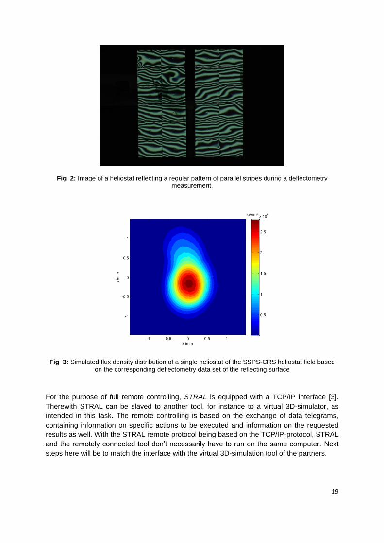
The deflectometry data of a single heliostat consists of a set of normal vectors located at

predefined raster points on the reflecting surface of the heliostat facets with a resolution of up

to 40 000 points/m². The normal vectors are attained by detecting the reflected images of

various regular patterns by each individual heliostat (Fig. 2). The flux density calculations

based on deflectometry data (Fig. 3) are much more precisely and usually differ significantly

from those based on idealized concentrator models (e.g. circular normal distribution of slope

errors). So far, only few single heliostats of the SSPS-CRS field have been measured with

deflectometry. A measurement campaign for the whole field is planned for 2011.

Fig 1: Screenshot of STRAL showing the SSPS-CRS heliostat field

19

Fig 2: Image of a heliostat reflecting a regular pattern of parallel stripes during a deflectometry measurement.

x in m

y in

m

kW/m²

-1 -0.5 0 0.5 1

-1

-0.5

0

0.5

1

0.5

1

1.5

2

2.5

x 104

Fig 3: Simulated flux density distribution of a single heliostat of the SSPS-CRS heliostat field based on the corresponding deflectometry data set of the reflecting surface

For the purpose of full remote controlling, STRAL is equipped with a TCP/IP interface [3].

Therewith STRAL can be slaved to another tool, for instance to a virtual 3D-simulator, as

intended in this task. The remote controlling is based on the exchange of data telegrams,

containing information on specific actions to be executed and information on the requested

results as well. With the STRAL remote protocol being based on the TCP/IP-protocol, STRAL

and the remotely connected tool don’t necessarily have to run on the same computer. Next

steps here will be to match the interface with the virtual 3D-simulation tool of the partners.

20

References:

[1] Belhomme, B., Pitz-Paal, R., Schwarzbözl, P., Ulmer, S., A new fast Ray Tracing Tool for

High-Precision Simulation of Heliostat Fields, Journal of Solar Energy Engineering, 131(3),

2009

[2] Steffen Ulmer, Tobias Marz, Christoph Prahl, Wolfgang Reinalter, Boris Belhomme,

Automated high resolution measurement of heliostat slope errors, Solar Energy, In Press,

Corrected Proof, Available online 1 February 2010

[3] Ahlbrink, N., Belhomme, B., Pitz-Paal, R., Modeling and Simulation of a Solar Tower

Power Plant with Open Volumetric Air Receiver, In: Proceedings of the 7th Modelica

Conference, S. 695-693, Como, 2009

21

Optical model of central receiver heliostat field (WIS facility)

1. Optical design of a new field. For the design of a new field of heliostats, two codes are

available: one for positioning the heliostats in a cornfield array (CORN), and the other in radial

staggered array (RAST). Both of them can position the heliostats either in a tower surrounding

field, or in a north field. In both codes the predetermined land boundaries limit the field size.

2. Optical calculations of an existing field case. In cases where the field was designed using

previous codes, or when the coordinates of the heliostats in the field are known, the field

performance can be calculated by the code named TRASOL. This code is a ray tracing program

written based on a group of routines adapted from the old Sandia's ray tracing code named

MIRVAL, complemented by new routines. The output of TRASOL consists of the characteristics

(vector origin, unit vector of direction and the proper power) of all the rays that leave the heliostats

in the direction of the aim-point. Another code named ASTRAC receives these rays as input and

follows their optical path in the geometry of the receiver.

ASTRAC is a new ray tracing code which provides the flux distribution on the various parts

and components of the receiver. This program is very flexible; various receiver geometries can be

easily added to the existing geometries recognized by the code. Presently, ASTRAC can treat

various types of planar apertures such as rectangular, circular and ellipsoidal or non-planar

apertures: hyperboloidal, paraboloidal or spherical. Various types of concentrators such as

compound parabolic concentrator (CPC), conical concentrator, transparent concentrator with total

internal reflection (TRC), or cassegrainian concentrator can be positioned behind the aperture. The

CPC or TRC concentrators can be considered as ideal or approximated by one or more truncated

cones or pyramids or flat facets. If the concentrator is an ideal CPC or one of its possible

approximations, it is treated by a subroutine of ASTRAC. In case that the concentrator is

approximated by truncated cones or pyramids, or it is type of DTIRC, ASTRAC can solve the

transmission through these concentrators.

3. Radiative heat transfer in the receiver. The radiation heat transfer calculations are

performed in the frame of the zonal method and using the semi-gray approximation (code

SOLRAD). Another in-house available code is REFMETH which is dedicated to calculation of the

heat stored in the chemical reaction of methane reforming. This code interacts with SOLRAD using

a new and special convergence method we've developed.