Deliverable: D5.1.7.2 (L2.7.2) Tests of hardware and ... · PDF filethe OS installation as well as the network linking the nodes ... freefem++/3.16 lammps/7jun13 wrf/3.3 ... Tests

(ITEA2 09011)

Optimize HPC Applications on Heterogeneous Architectures

•••••••••••••••••••••••••••••••••••••••••••••••••••••••••••••••••••••••••••••••••••••••••

Deliverable: D5.1.7.2 (L2.7.2)

Tests of hardware and software developments

Version: V1.0

Date: 05/01/15

Authors: CEA/DAM / Guillaume Colin de VERDIERE,

Dassault Aviation / Quang Vinh DINH

Status: Draft

Visibility: Public

D5.1.7.2 - Tests of hardware and software developments

V1.0 - 05/01/15 - Draft - Public

CEA/DAM Page 2 / 23

F

i

g

u

r

e

E

r

r

o

r

!

M

a

i

n

D

o

c

u

m

e

n

t

O

n

l

y

.

HISTORY

Document version #

Date Remarks Author

V0.0 15/12/14 Initial version G. Colin de Verdière

V0.1 16/12/14 UVSQ review taken into account G. Colin de Verdière

V0.2 16/12/14 Tests of the accelerator section G. Colin de Verdière

V0.3 23/12/14 Dassault Aviation contribution Q. V. Dinh

V1.0 05/01/15 Prototype usage G. Colin de Verdière


V1.0 - 05/01/15 - Draft - Public

CEA/DAM Page 3 / 23

F

i

g

u

r

e

E

r

r

o

r

!

M

a

i

n

D

o

c

u

m

e

n

t

O

n

l

y

.

TABLE OF CONTENTS

1 Summary ................................................................................................................................................................... 4

2 Introduction ................................................................................................................................................................ 4

3 Specific tests ............................................................................................................................................................. 4

3.1 Code selected ...................................................................................................................... 4

3.2 Basic test of the machine ..................................................................................................... 4

3.3 Test of the accelerator ......................................................................................................... 8

3.4 Test of the CAPS developments......................................................................................... 10

3.5 Test of the UVSQ developments ........................................................................................ 10

3.6 Usage of the prototype ....................................................................................................... 14

4 A more elaborate benchmark .................................................................................................................................15

4.1 Relations with the initial H4H project .................................................................................. 15

4.2 Technical description: a CFD software and its derived FEM mini-application ...................... 16

4.2.1 Introducing D&C in AeTHER ........................................................................................... 16

4.2.2 The FEM mini-application ............................................................................................... 19

4.3 Benchmark results on the FEM mini-application ................................................................. 20

5 Abbreviations and acronyms ..................................................................................................................................23

6 References ..............................................................................................................................................................23


V1.0 - 05/01/15 - Draft - Public

CEA/DAM Page 4 / 23

F

i

g

u

r

e

E

r

r

o

r

!

M

a

i

n

D

o

c

u

m

e

n

t

O

n

l

y

.

1 Summary

This deliverable is the implementation of the tests specification described in deliverable D5.1.7.1. It

covers basic functional tests of the Cirrus platform, tests of its accelerator component, a more

elaborate benchmark by the Dassault Aviation (DA) partner and a specific focus on the tools

developed by the UVSQ partner.

2 Introduction

This deliverable describes the results of the tests specified in deliverable D5.1.7.1, which were

accomplished through a collaborative work between the partners CEA, DA and UVSQ. In this

deliverable we will first show that the prototype of an accelerator-based architecture, namely the Cirrus

platform, is functional, second that it is performant on different use cases and third that tools

developed by the UVSQ partner can help to optimize codes on such an architecture.

In addition, we will describe a more elaborate investigation allowed by the prototype. This benchmark

involves a full FEM mini-application using industrial-grade simulation data, provided by DA. Even

though it was not funded during the November 2013 – December 2014 time period of the

H4H/Perfcloud project, DA was willing to participate in order to test its mini-application on the Xeon Phi

architecture of the Cirrus platform.

3 Specific tests

3.1 Code selected

To test the machines as well as the environments, we used the Hydro benchmark [Github].

This basic benchmark is available in a number of implementations allowing for rapid evaluation of a platform, be it a single node or a cluster with or without acceleration.

3.2 Basic test of the machine

The first test will be to use the OpenCL + MPI version of Hydro. It should produce the same output as on a production cluster. The output should be identical on the first 10 iterations. This run will validate the OS installation as well as the network linking the nodes (if any).

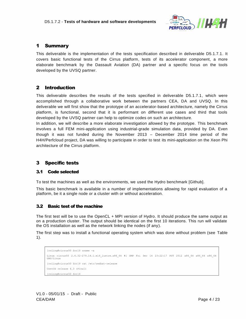
The first step was to install a functional operating system which was done without problem (see Table 1).

[coling@cirrus50 Src]$ uname -a

Linux cirrus50 2.6.32-279.14.1.el6_lustre.x86_64 #1 SMP Fri Dec 14 23:22:17 PST 2012 x86_64 x86_64 x86_64

GNU/Linux

[coling@cirrus50 Src]$ cat /etc/redhat-release

CentOS release 6.3 (Final)

[coling@cirrus50 Src]$


V1.0 - 05/01/15 - Draft - Public

CEA/DAM Page 5 / 23

F

i

g

u

r

e

E

r

r

o

r

!

M

a

i

n

D

o

c

u

m

e

n

t

O

n

l

y

.

Table 1: Operating system of the Cirrus prototype

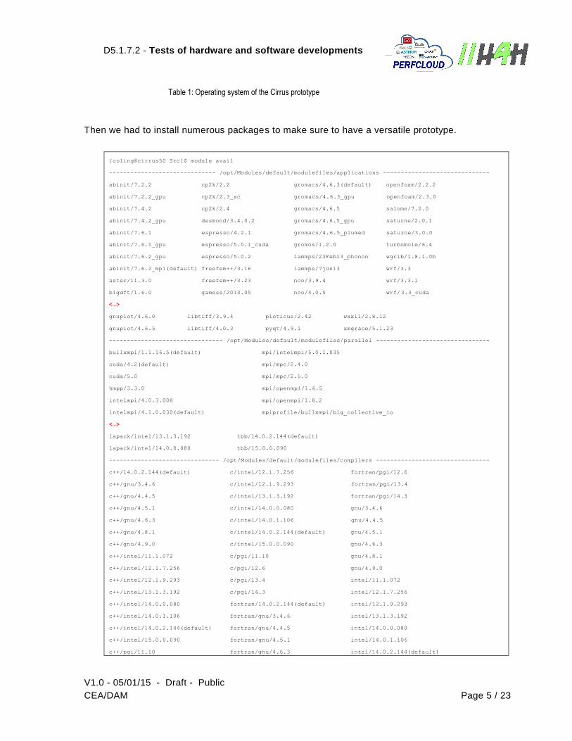
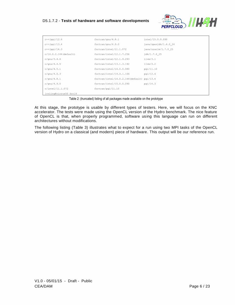
Then we had to install numerous packages to make sure to have a versatile prototype.

[coling@cirrus50 Src]$ module avail

------------------------------ /opt/Modules/default/modulefiles/applications ------------------------------

abinit/7.2.2 cp2k/2.2 gromacs/4.6.3(default) openfoam/2.2.2

abinit/7.2.2_gpu cp2k/2.3_xc gromacs/4.6.3_gpu openfoam/2.3.0

abinit/7.4.2 cp2k/2.4 gromacs/4.6.5 salome/7.2.0

abinit/7.4.2_gpu desmond/3.4.0.2 gromacs/4.6.5_gpu saturne/2.0.1

abinit/7.6.1 espresso/4.2.1 gromacs/4.6.5_plumed saturne/3.0.0

abinit/7.6.1_gpu espresso/5.0.1_cuda gromos/1.2.0 turbomole/6.4

abinit/7.6.2_gpu espresso/5.0.2 lammps/23Feb13_phonon wgrib/1.8.1.0b

abinit/7.6.2_mpi(default) freefem++/3.16 lammps/7jun13 wrf/3.3

aster/11.3.0 freefem++/3.23 nco/3.9.4 wrf/3.3.1

bigdft/1.6.0 gamess/2013.05 nco/4.0.5 wrf/3.3_cuda

<…>

gnuplot/4.6.0 libtiff/3.9.4 ploticus/2.42 wxx11/2.8.12

gnuplot/4.6.5 libtiff/4.0.3 pyqt/4.9.1 xmgrace/5.1.23

-------------------------------- /opt/Modules/default/modulefiles/parallel --------------------------------

bullxmpi/1.1.16.5(default) mpi/intelmpi/5.0.1.035

cuda/4.2(default) mpi/mpc/2.4.0

cuda/5.0 mpi/mpc/2.5.0

hmpp/3.3.0 mpi/openmpi/1.6.5

intelmpi/4.0.3.008 mpi/openmpi/1.8.2

intelmpi/4.1.0.030(default) mpiprofile/bullxmpi/big_collective_io

<…>

lapack/intel/13.1.3.192 tbb/14.0.2.144(default)

lapack/intel/14.0.0.080 tbb/15.0.0.090

------------------------------- /opt/Modules/default/modulefiles/compilers --------------------------------

c++/14.0.2.144(default) c/intel/12.1.7.256 fortran/pgi/12.6

c++/gnu/3.4.6 c/intel/12.1.9.293 fortran/pgi/13.4

c++/gnu/4.4.5 c/intel/13.1.3.192 fortran/pgi/14.3

c++/gnu/4.5.1 c/intel/14.0.0.080 gnu/3.4.6

c++/gnu/4.6.3 c/intel/14.0.1.106 gnu/4.4.5

c++/gnu/4.8.1 c/intel/14.0.2.144(default) gnu/4.5.1

c++/gnu/4.9.0 c/intel/15.0.0.090 gnu/4.6.3

c++/intel/11.1.072 c/pgi/11.10 gnu/4.8.1

c++/intel/12.1.7.256 c/pgi/12.6 gnu/4.9.0

c++/intel/12.1.9.293 c/pgi/13.4 intel/11.1.072

c++/intel/13.1.3.192 c/pgi/14.3 intel/12.1.7.256

c++/intel/14.0.0.080 fortran/14.0.2.144(default) intel/12.1.9.293

c++/intel/14.0.1.106 fortran/gnu/3.4.6 intel/13.1.3.192

c++/intel/14.0.2.144(default) fortran/gnu/4.4.5 intel/14.0.0.080

c++/intel/15.0.0.090 fortran/gnu/4.5.1 intel/14.0.1.106

c++/pgi/11.10 fortran/gnu/4.6.3 intel/14.0.2.144(default)


V1.0 - 05/01/15 - Draft - Public

CEA/DAM Page 6 / 23

F

i

g

u

r

e

E

r

r

o

r

!

M

a

i

n

D

o

c

u

m

e

n

t

O

n

l

y

.

c++/pgi/12.6 fortran/gnu/4.8.1 intel/15.0.0.090

c++/pgi/13.4 fortran/gnu/4.9.0 java/openjdk/1.6.0_24

c++/pgi/14.3 fortran/intel/11.1.072 java/oracle/1.7.0_25

c/14.0.2.144(default) fortran/intel/12.1.7.256 jdk/1.7.0_25

c/gnu/3.4.6 fortran/intel/12.1.9.293 llvm/3.1

c/gnu/4.4.5 fortran/intel/13.1.3.192 llvm/3.2

c/gnu/4.5.1 fortran/intel/14.0.0.080 pgi/11.10


c/gnu/4.8.1 fortran/intel/14.0.2.144(default) pgi/13.4


c/intel/11.1.072 fortran/pgi/11.10

[coling@cirrus50 Src]$

Table 2: (truncated) listing of all packages made available on the prototype

At this stage, the prototype is usable by different types of testers. Here, we will focus on the KNC accelerator. The tests were made using the OpenCL version of the Hydro benchmark. The nice feature of OpenCL is that, when properly programmed, software using this language can run on different architectures without modifications.

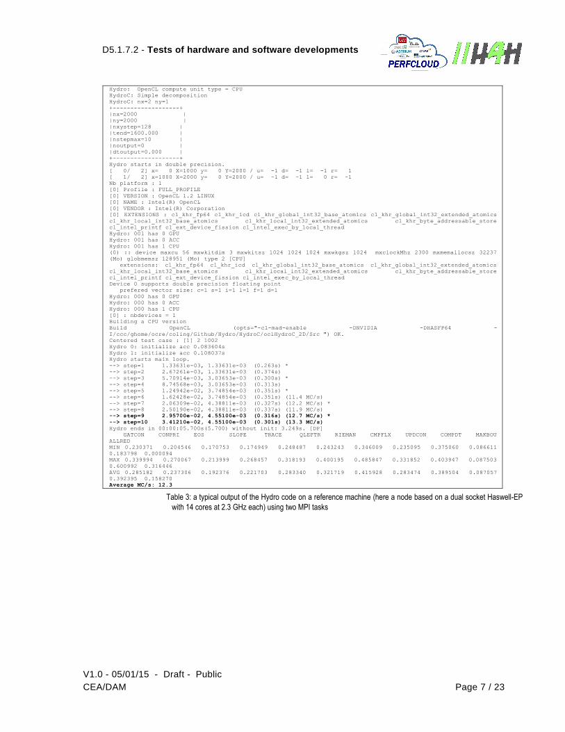
The following listing (Table 3) illustrates what to expect for a run using two MPI tasks of the OpenCL version of Hydro on a classical (and modern) piece of hardware. This output will be our reference run.


V1.0 - 05/01/15 - Draft - Public

CEA/DAM Page 7 / 23

F

i

g

u

r

e

E

r

r

o

r

!

M

a

i

n

D

o

c

u

m

e

n

t

O

n

l

y

.

Hydro: OpenCL compute unit type = CPU

HydroC: Simple decomposition

HydroC: nx=2 ny=1

+-------------------+

|nx=2000 |

|ny=2000 |

|nxystep=128 |

|tend=1600.000 |

|nstepmax=10 |

|noutput=0 |

|dtoutput=0.000 |

+-------------------+

Hydro starts in double precision.

[ 0/ 2] x= 0 X=1000 y= 0 Y=2000 / u= -1 d= -1 l= -1 r= 1

[ 1/ 2] x=1000 X=2000 y= 0 Y=2000 / u= -1 d= -1 l= 0 r= -1

Nb platform : 1

[0] Profile : FULL_PROFILE

[0] VERSION : OpenCL 1.2 LINUX

[0] NAME : Intel(R) OpenCL

[0] VENDOR : Intel(R) Corporation

[0] EXTENSIONS : cl_khr_fp64 cl_khr_icd cl_khr_global_int32_base_atomics cl_khr_global_int32_extended_atomics

cl_khr_local_int32_base_atomics cl_khr_local_int32_extended_atomics cl_khr_byte_addressable_store

cl_intel_printf cl_ext_device_fission cl_intel_exec_by_local_thread

Hydro: 001 has 0 GPU

Hydro: 001 has 0 ACC

Hydro: 001 has 1 CPU

(0) :: device maxcu 56 mxwkitdim 3 mxwkitsz 1024 1024 1024 mxwkgsz 1024 mxclockMhz 2300 mxmemallocsz 32237

(Mo) globmemsz 128951 (Mo) type 2 [CPU]

extensions: cl_khr_fp64 cl_khr_icd cl_khr_global_int32_base_atomics cl_khr_global_int32_extended_atomics

cl_khr_local_int32_base_atomics cl_khr_local_int32_extended_atomics cl_khr_byte_addressable_store

cl_intel_printf cl_ext_device_fission cl_intel_exec_by_local_thread

Device 0 supports double precision floating point

prefered vector size: c=1 s=1 i=1 l=1 f=1 d=1



Hydro: 000 has 1 CPU

[0] : nbdevices = 1

Building a CPU version

Build OpenCL (opts="-cl-mad-enable -DNVIDIA -DHASFP64 -

I/ccc/ghome/ocre/coling/Github/Hydro/HydroC/oclHydroC_2D/Src ") OK.

Centered test case : [1] 2 1002

Hydro 0: initialize acc 0.083604s


Hydro starts main loop.

--> step=1 1.33631e-03, 1.33631e-03 (0.263s) *

--> step=2 2.67261e-03, 1.33631e-03 (0.374s)

--> step=3 5.70914e-03, 3.03653e-03 (0.300s) *

--> step=4 8.74568e-03, 3.03653e-03 (0.313s)

--> step=5 1.24942e-02, 3.74854e-03 (0.351s) *

--> step=6 1.62428e-02, 3.74854e-03 (0.351s) (11.4 MC/s)

--> step=7 2.06309e-02, 4.38811e-03 (0.327s) (12.2 MC/s) *

--> step=8 2.50190e-02, 4.38811e-03 (0.337s) (11.9 MC/s)

--> step=9 2.95700e-02, 4.55100e-03 (0.316s) (12.7 MC/s) *

--> step=10 3.41210e-02, 4.55100e-03 (0.301s) (13.3 MC/s)

Hydro ends in 00:00:05.700s(5.700) without init: 3.249s. [DP]

GATCON CONPRI EOS SLOPE TRACE QLEFTR RIEMAN CMPFLX UPDCON COMPDT MAKBOU

ALLRED

MIN 0.230371 0.204546 0.170753 0.174949 0.248487 0.243243 0.346009 0.235095 0.375060 0.086611

0.183798 0.000094

MAX 0.339994 0.270067 0.213999 0.268457 0.318193 0.400195 0.485847 0.331852 0.403947 0.087503

0.600992 0.316446

AVG 0.285182 0.237306 0.192376 0.221703 0.283340 0.321719 0.415928 0.283474 0.389504 0.087057

0.392395 0.158270

Average MC/s: 12.3

Table 3: a typical output of the Hydro code on a reference machine (here a node based on a dual socket Haswell-EP

with 14 cores at 2.3 GHz each) using two MPI tasks


V1.0 - 05/01/15 - Draft - Public

CEA/DAM Page 8 / 23

F

i

g

u

r

e

E

r

r

o

r

!

M

a

i

n

D

o

c

u

m

e

n

t

O

n

l

y

.

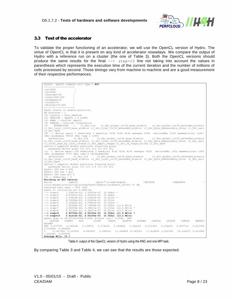
3.3 Test of the accelerator

To validate the proper functioning of an accelerator, we will use the OpenCL version of Hydro. The virtue of OpenCL is that it is present on any kind of accelerator nowadays. We compare the output of Hydro with a reference run on a cluster (the one of Table 3). Both the OpenCL versions should

produce the same results for the final --> step=10 line not taking into account the values in

parenthesis which represents the execution time of the current iteration and the number of millions of cells processed by second. Those timings vary from machine to machine and are a good measurement of their respective performances.

Hydro: OpenCL compute unit type = ACC

+-------------------+

|nx=2000 |

|ny=2000 |

|nxystep=128 |

|tend=1600.000 |

|nstepmax=10 |

|noutput=0 |

|dtoutput=0.000 |

+-------------------+

Hydro starts in double precision.

Nb platform : 1

[0] Profile : FULL_PROFILE

[0] VERSION : OpenCL 1.2 LINUX

[0] NAME : Intel(R) OpenCL

[0] VENDOR : Intel(R) Corporation

[0] EXTENSIONS : cl_khr_icd cl_khr_global_int32_base_atomics cl_khr_global_int32_extended_atomics

cl_khr_local_int32_base_atomics cl_khr_local_int32_extended_atomics cl_khr_byte_addressable_store cl_khr_spir

cl_khr_fp64


(Mo) globmemsz 48230 (Mo) type 2 [CPU]

extensions: cl_khr_icd cl_khr_global_int32_base_atomics cl_khr_global_int32_extended_atomics


cl_intel_exec_by_local_thread cl_khr_depth_images cl_khr_3d_image_writes cl_khr_fp64

Device 0 supports double precision floatting point



(Mo) globmemsz 5773 (Mo) type 8 [ACCELERATOR]

extensions: cl_khr_icd cl_khr_global_int32_base_atomics cl_khr_global_int32_extended_atomics


cl_khr_fp64

Device 1 supports double precision floating point




Hydro: 000 uses ACC 0

[0] : nbdevices = 2

Building an ACC version

Build OpenCL (opts="-cl-mad-enable -DNVIDIA -DHASFP64 -

I/ccc/ghome/ocre/coling/Github/Hydro/HydroC/oclHydroC_2D/Src ") OK.

Centered test case : 1002 1002


--> step=1 1.33631e-03, 1.33631e-03 (0.364s) *

--> step=2 2.67261e-03, 1.33631e-03 (0.304s)

--> step=3 5.70914e-03, 3.03653e-03 (0.361s) *

--> step=4 8.74568e-03, 3.03653e-03 (0.301s)

--> step=5 1.24942e-02, 3.74854e-03 (0.332s) *

--> step=6 1.62428e-02, 3.74854e-03 (0.308s) (13.0 MC/s)

--> step=7 2.06309e-02, 4.38811e-03 (0.333s) (12.0 MC/s) *

--> step=8 2.50190e-02, 4.38811e-03 (0.301s) (13.3 MC/s)

--> step=9 2.95700e-02, 4.55100e-03 (0.336s) (11.9 MC/s) *

--> step=10 3.41210e-02, 4.55100e-03 (0.302s) (13.2 MC/s)



ALLRED

PE0 0.577700 0.166104 0.129874 0.174436 0.365882 0.264103 0.571189 0.169403 0.587714 0.201799

0.034090 0.000000

% 17.817641 5.123032 4.005629 5.380016 11.284665 8.145553 17.616830 5.224789 18.126475 6.223969

1.051401 0.000000

Average MC/s: 12.7

Table 4: output of the OpenCL version of Hydro using the KNC and one MPI task.

By comparing Table 3 and Table 4, we can see that the results are those expected.


V1.0 - 05/01/15 - Draft - Public

CEA/DAM Page 9 / 23

F

i

g

u

r

e

E

r

r

o

r

!

M

a

i

n

D

o

c

u

m

e

n

t

O

n

l

y

.

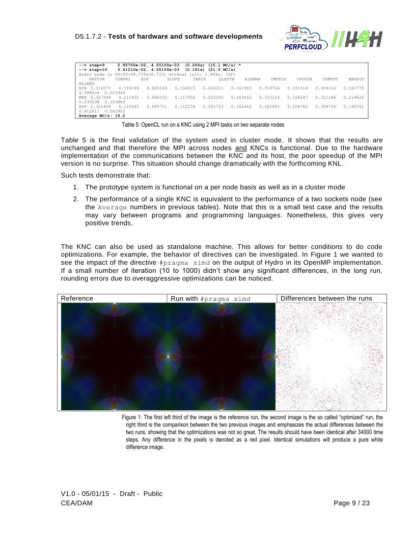
--> step=9 2.95700e-02, 4.55100e-03 (0.266s) (15.1 MC/s) *

--> step=10 3.41210e-02, 4.55100e-03 (0.191s) (21.0 MC/s)



ALLRED

MIN 0.316271 0.109199 0.085169 0.106515 0.200221 0.161903 0.318756 0.101318 0.306316 0.161775

0.395536 0.023942

MAX 0.327046 0.111931 0.086332 0.117952 0.203285 0.163022 0.333114 0.108247 0.311196 0.219626

0.430098 0.103863

AVG 0.321658 0.110565 0.085751 0.112234 0.201753 0.162462 0.325935 0.104782 0.308756 0.190701

0.412817 0.063903

Average MC/s: 18.2

Table 5: OpenCL run on a KNC using 2 MPI tasks on two separate nodes

Table 5 is the final validation of the system used in cluster mode. It shows that the results are unchanged and that therefore the MPI across nodes and KNCs is functional. Due to the hardware implementation of the communications between the KNC and its host, the poor speedup of the MPI version is no surprise. This situation should change dramatically with the forthcoming KNL.

Such tests demonstrate that:

1. The prototype system is functional on a per node basis as well as in a cluster mode

2. The performance of a single KNC is equivalent to the performance of a two sockets node (see

the Average numbers in previous tables). Note that this is a small test case and the results

may vary between programs and programming languages. Nonetheless, this gives very positive trends.

The KNC can also be used as standalone machine. This allows for better conditions to do code optimizations. For example, the behavior of directives can be investigated. In Figure 1 we wanted to

see the impact of the directive #pragma simd on the output of Hydro in its OpenMP implementation.

If a small number of iteration (10 to 1000) didn’t show any significant differences, in the long run, rounding errors due to overaggressive optimizations can be noticed.

Reference Run with #pragma simd Differences between the runs

Figure 1: The first left third of the image is the reference run, the second image is the so called “optimized” run, the

right third is the comparison between the two previous images and emphasizes the actual differences between the

two runs, showing that the optimizations was not so great. The results should have been identical after 34000 time

steps. Any difference in the pixels is denoted as a red pixel. Identical simulations will produce a pure white

difference image.


V1.0 - 05/01/15 - Draft - Public

CEA/DAM Page 10 / 23

F

i

g

u

r

e

E

r

r

o

r

!

M

a

i

n

D

o

c

u

m

e

n

t

O

n

l

y

.

3.4 Test of the CAPS developments

Because the CAPS partner had to withdraw from the project, no tests were made of their developments.

3.5 Test of the UVSQ developments

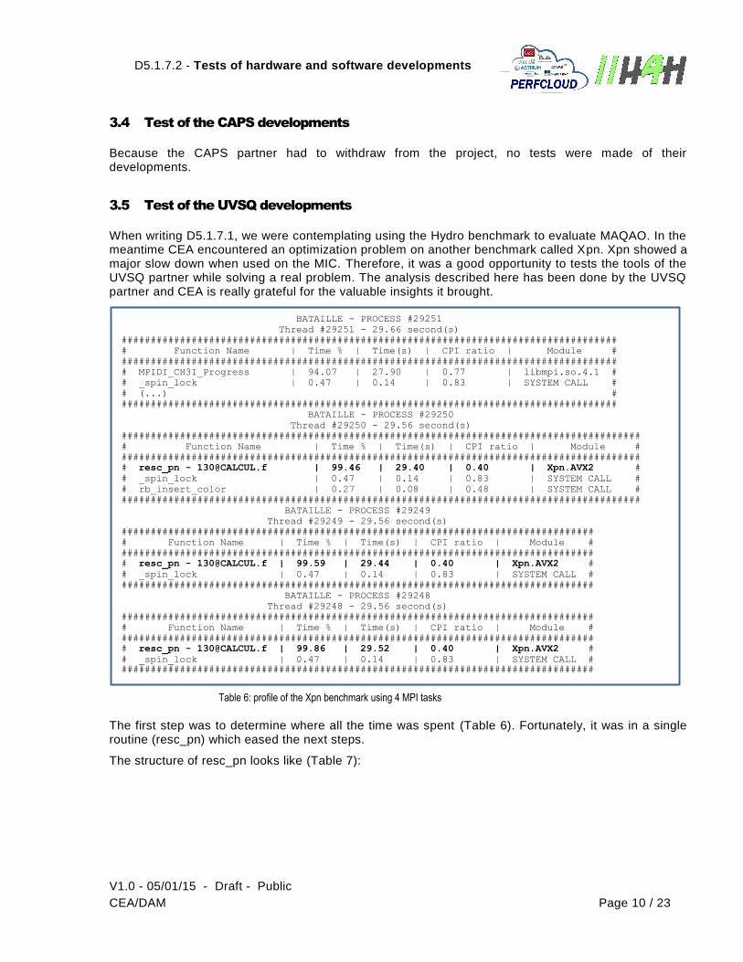
When writing D5.1.7.1, we were contemplating using the Hydro benchmark to evaluate MAQAO. In the meantime CEA encountered an optimization problem on another benchmark called Xpn. Xpn showed a major slow down when used on the MIC. Therefore, it was a good opportunity to tests the tools of the UVSQ partner while solving a real problem. The analysis described here has been done by the UVSQ partner and CEA is really grateful for the valuable insights it brought.

Table 6: profile of the Xpn benchmark using 4 MPI tasks

The first step was to determine where all the time was spent (Table 6). Fortunately, it was in a single routine (resc_pn) which eased the next steps.

The structure of resc_pn looks like (Table 7):

BATAILLE - PROCESS #29251

Thread #29251 - 29.66 second(s)

#####################################################################################

# Function Name | Time % | Time(s) | CPI ratio | Module #

#####################################################################################

# MPIDI_CH3I_Progress | 94.07 | 27.90 | 0.77 | libmpi.so.4.1 #

# _spin_lock | 0.47 | 0.14 | 0.83 | SYSTEM CALL #

# (...) #

#####################################################################################



#########################################################################################


#########################################################################################

# resc_pn - [email protected] | 99.46 | 29.40 | 0.40 | Xpn.AVX2 #


# rb_insert_color | 0.27 | 0.08 | 0.48 | SYSTEM CALL #

#########################################################################################



#################################################################################


#################################################################################



#################################################################################



#################################################################################


#################################################################################



#################################################################################


V1.0 - 05/01/15 - Draft - Public


F

i

g

u

r

e

E

r

r

o

r

!

M

a

i

n

D

o

c

u

m

e

n

t

O

n

l

y

.

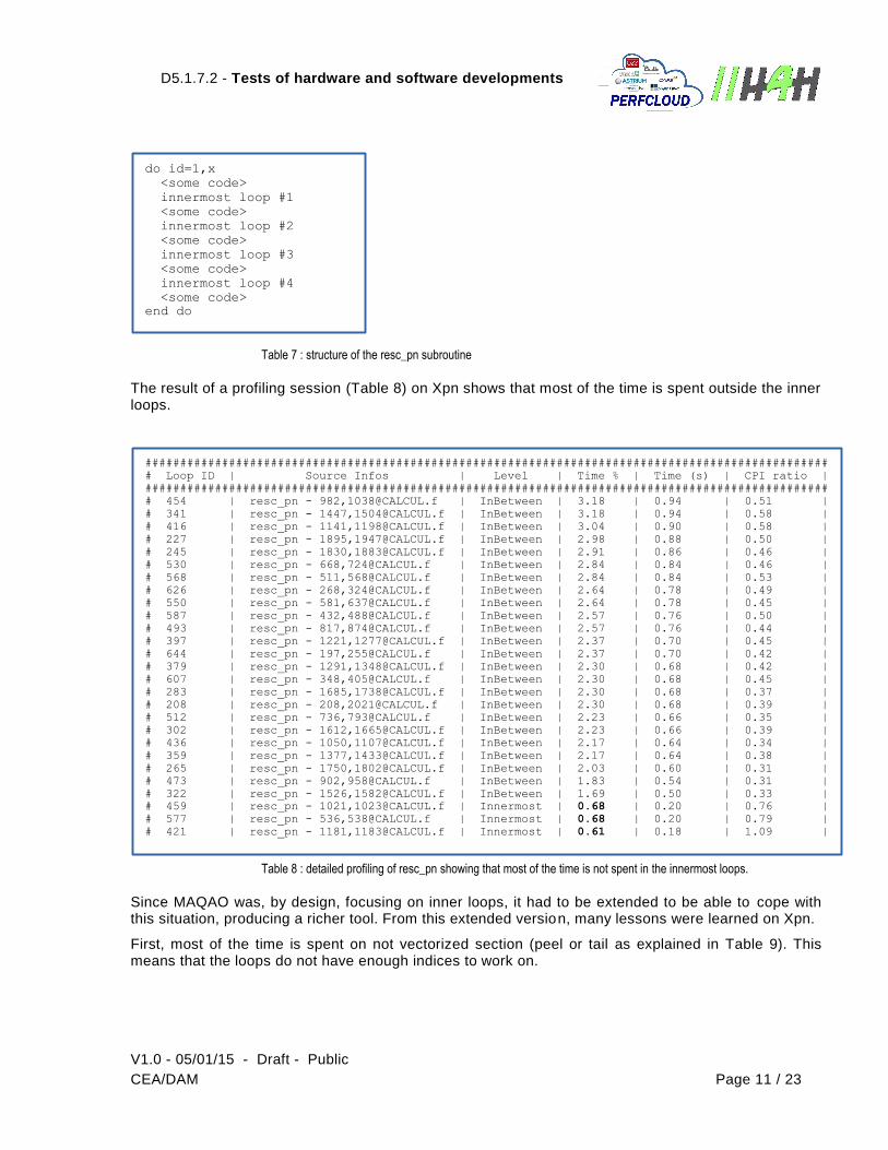
Table 7 : structure of the resc_pn subroutine

The result of a profiling session (Table 8) on Xpn shows that most of the time is spent outside the inner loops.

Table 8 : detailed profiling of resc_pn showing that most of the time is not spent in the innermost loops.

Since MAQAO was, by design, focusing on inner loops, it had to be extended to be able to cope with this situation, producing a richer tool. From this extended version, many lessons were learned on Xpn.

First, most of the time is spent on not vectorized section (peel or tail as explained in Table 9). This means that the loops do not have enough indices to work on.

do id=1,x

<some code>

innermost loop #1

<some code>

innermost loop #2

<some code>

innermost loop #3

<some code>

innermost loop #4

<some code>

end do

##################################################################################################

# Loop ID | Source Infos | Level | Time % | Time (s) | CPI ratio |

##################################################################################################

# 454 | resc_pn - 982,[email protected] | InBetween | 3.18 | 0.94 | 0.51 |
























# 459 | resc_pn - 1021,[email protected] | Innermost | 0.68 | 0.20 | 0.76 |




V1.0 - 05/01/15 - Draft - Public


F

i

g

u

r

e

E

r

r

o

r

!

M

a

i

n

D

o

c

u

m

e

n

t

O

n

l

y

.

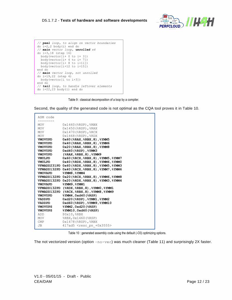
Table 9 : classical decomposition of a loop by a compiler.

Second, the quality of the generated code is not optimal as the CQA tool proves it in Table 10.

Table 10 : generated assembly code using the default (-O3) optimizing options.

The not vectorized version (option –no-vec) was much cleaner (Table 11) and surprisingly 2X faster.

// peel loop, to align on vector boundaries

do i=2,2 body(i) end do

// main vector loop, unrolled x4

do i=3,18 (step 16)

body(vector[i+ 0 to i+ 3])

body(vector[i+ 4 to i+ 7])

body(vector[i+ 8 to i+11])

body(vector[i+12 to i+15])

end do

// main vector loop, not unrolled

do i=19,22 (step 4)

body(vector[i to i+3])

end do

// tail loop, to handle leftover elements do i=22,23 body(i) end do

ASM code

--------

MOV 0x1460(%RSP),%RBX

MOV 0x1450(%RSP),%RAX

MOV 0x1470(%RSP),%RCX

MOV 0x1468(%RSP),%RDX

VMOVUPD 0x60(%RAX,%RBX,8),%YMM5



VMOVUPD 0xd40(%RSP),%YMM3

VMOVUPD (%RAX,%RBX,8),%YMM9

VMULPD 0x60(%RCX,%RBX,8),%YMM5,%YMM7

VMULPD 0x40(%RDX,%RBX,8),%YMM6,%YMM0

VFMADD231PD 0x60(%RDX,%RBX,8),%YMM5,%YMM3

VFMADD132PD 0x40(%RCX,%RBX,8),%YMM7,%YMM6

VMOVAPD %YMM8,%YMM4

VFMADD132PD 0x20(%RCX,%RBX,8),%YMM6,%YMM8

VFMADD132PD 0x20(%RDX,%RBX,8),%YMM3,%YMM4

VMOVAPD %YMM9,%YMM1

VFMADD132PD (%RDX,%RBX,8),%YMM0,%YMM1

VFMADD132PD (%RCX,%RBX,8),%YMM8,%YMM9

VMOVUPD %YMM4,0xd40(%RSP)

VADDPD 0xd20(%RSP),%YMM1,%YMM2

VADDPD 0xd60(%RSP),%YMM9,%YMM10

VMOVUPS %YMM2,0xd20(%RSP)

VMOVUPS %YMM10,0xd60(%RSP)

ADD $0x10,%RBX

MOV %RBX,0x1460(%RSP)

CMP 0x1478(%RSP),%RBX

JB 417ad5 <resc_pn_+0x3555>


V1.0 - 05/01/15 - Draft - Public


F

i

g

u

r

e

E

r

r

o

r

!

M

a

i

n

D

o

c

u

m

e

n

t

O

n

l

y

.

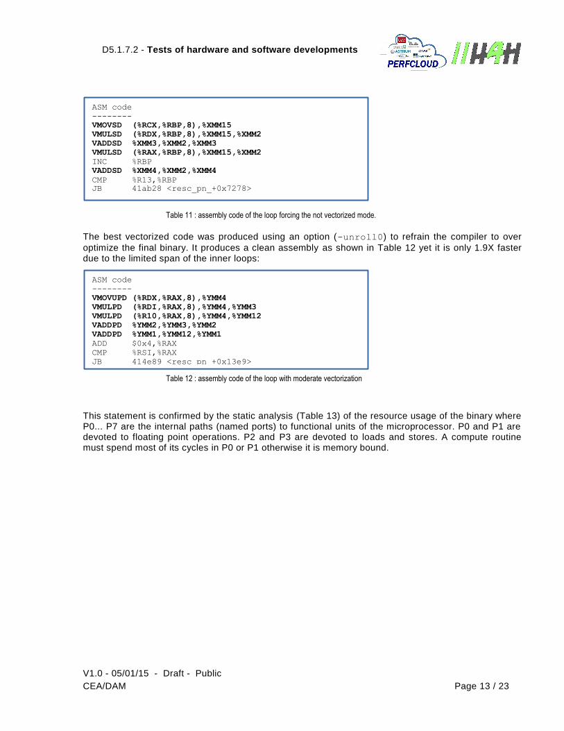
Table 11 : assembly code of the loop forcing the not vectorized mode.

The best vectorized code was produced using an option (-unroll0) to refrain the compiler to over

optimize the final binary. It produces a clean assembly as shown in Table 12 yet it is only 1.9X faster due to the limited span of the inner loops:

Table 12 : assembly code of the loop with moderate vectorization

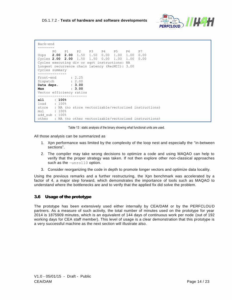
This statement is confirmed by the static analysis (Table 13) of the resource usage of the binary where P0... P7 are the internal paths (named ports) to functional units of the microprocessor. P0 and P1 are devoted to floating point operations. P2 and P3 are devoted to loads and stores. A compute routine must spend most of its cycles in P0 or P1 otherwise it is memory bound.

ASM code

--------

VMOVSD (%RCX,%RBP,8),%XMM15

VMULSD (%RDX,%RBP,8),%XMM15,%XMM2

VADDSD %XMM3,%XMM2,%XMM3

VMULSD (%RAX,%RBP,8),%XMM15,%XMM2

INC %RBP

VADDSD %XMM4,%XMM2,%XMM4

CMP %R13,%RBP

JB 41ab28 <resc_pn_+0x7278>

ASM code

--------

VMOVUPD (%RDX,%RAX,8),%YMM4

VMULPD (%RDI,%RAX,8),%YMM4,%YMM3

VMULPD (%R10,%RAX,8),%YMM4,%YMM12

VADDPD %YMM2,%YMM3,%YMM2

VADDPD %YMM1,%YMM12,%YMM1

ADD $0x4,%RAX

CMP %RSI,%RAX

JB 414e89 <resc_pn_+0x13e9>


V1.0 - 05/01/15 - Draft - Public


F

i

g

u

r

e

E

r

r

o

r

!

M

a

i

n

D

o

c

u

m

e

n

t

O

n

l

y

.

Table 13 : static analysis of the binary showing what functional units are used.

All those analysis can be summarized as

1. Xpn performance was limited by the complexity of the loop nest and especially the “in-between sections”.

2. The compiler may take wrong decisions to optimize a code and using MAQAO can help to verify that the proper strategy was taken. If not then explore other non-classical approaches

such as the –unroll0 option.

3. Consider reorganizing the code in depth to promote longer vectors and optimize data locality.

Using the previous remarks and a further restructuring, the Xpn benchmark was accelerated by a factor of 4, a major step forward, which demonstrates the importance of tools such as MAQAO to understand where the bottlenecks are and to verify that the applied fix did solve the problem.

3.6 Usage of the prototype

The prototype has been extensively used either internally by CEA/DAM or by the PERFCLOUD partners. As a measure of such activity, the total number of minutes used on the prototype for year 2014 is 1875909 minutes, which is an equivalent of 144 days of continuous work per node (out of 192 working days for CEA staff member). This level of usage is a clear demonstration that this prototype is a very successful machine as the next section will illustrate also.

Back-end

--------

P0 P1 P2 P3 P4 P5 P6 P7

Uops 2.00 2.00 1.50 1.50 0.00 1.00 1.00 0.00

Cycles 2.00 2.00 1.50 1.50 0.00 1.00 1.00 0.00

Cycles executing div or sqrt instructions: NA

Longest recurrence chain latency (RecMII): 3.00

Cycles summary

--------------

Front-end : 2.25

Dispatch : 2.00

Data deps. : 3.00

Max : 3.00

Vector efficiency ratios

------------------------

all : 100%

load : 100%

store : NA (no store vectorizable/vectorized instructions)

mul : 100%

add_sub : 100%

other : NA (no other vectorizable/vectorized instructions)


V1.0 - 05/01/15 - Draft - Public


F

i

g

u

r

e

E

r

r

o

r

!

M

a

i

n

D

o

c

u

m

e

n

t

O

n

l

y

.

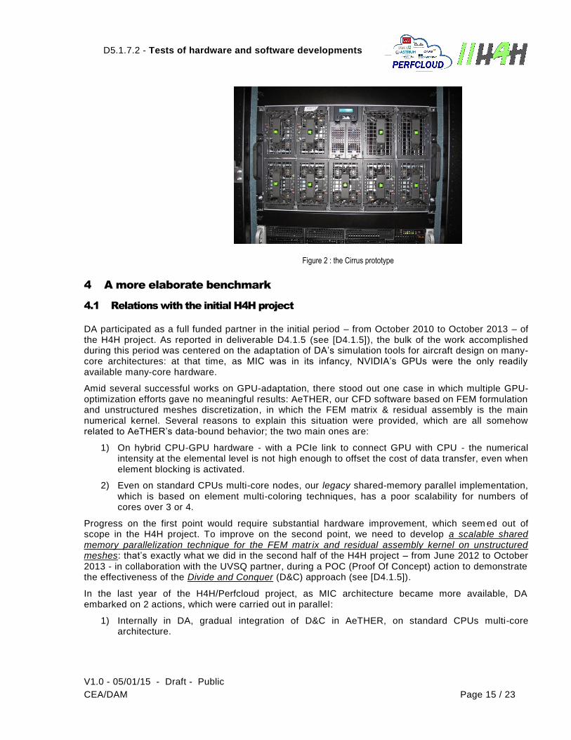
Figure 2 : the Cirrus prototype

4 A more elaborate benchmark

4.1 Relations with the initial H4H project

DA participated as a full funded partner in the initial period – from October 2010 to October 2013 – of the H4H project. As reported in deliverable D4.1.5 (see [D4.1.5]), the bulk of the work accomplished during this period was centered on the adaptation of DA’s simulation tools for aircraft design on many-core architectures: at that time, as MIC was in its infancy, NVIDIA’s GPUs were the only readily available many-core hardware.

Amid several successful works on GPU-adaptation, there stood out one case in which multiple GPU-optimization efforts gave no meaningful results: AeTHER, our CFD software based on FEM formulation and unstructured meshes discretization, in which the FEM matrix & residual assembly is the main numerical kernel. Several reasons to explain this situation were provided, which are all somehow related to AeTHER’s data-bound behavior; the two main ones are:

1) On hybrid CPU-GPU hardware - with a PCIe link to connect GPU with CPU - the numerical intensity at the elemental level is not high enough to offset the cost of data transfer, even when element blocking is activated.

2) Even on standard CPUs multi-core nodes, our legacy shared-memory parallel implementation, which is based on element multi-coloring techniques, has a poor scalability for numbers of cores over 3 or 4.

Progress on the first point would require substantial hardware improvement, which seem ed out of scope in the H4H project. To improve on the second point, we need to develop a scalable shared memory parallelization technique for the FEM matrix and residual assembly kernel on unstructured meshes: that’s exactly what we did in the second half of the H4H project – from June 2012 to October 2013 - in collaboration with the UVSQ partner, during a POC (Proof Of Concept) action to demonstrate the effectiveness of the Divide and Conquer (D&C) approach (see [D4.1.5]).

In the last year of the H4H/Perfcloud project, as MIC architecture became more available, DA embarked on 2 actions, which were carried out in parallel:

1) Internally in DA, gradual integration of D&C in AeTHER, on standard CPUs multi-core architecture.


V1.0 - 05/01/15 - Draft - Public


F

i

g

u

r

e

E

r

r

o

r

!

M

a

i

n

D

o

c

u

m

e

n

t

O

n

l

y

.

2) In the H4H/Perfcloud project, test of the D&C approach on the MIC architecture, which is available on the Cirrus prototype.

In what follows, we will first recall AeTHER’s MPI implementation and some of the D&C integration work, as well as how the FEM mini-application was derived. Finally, we will report on the benchmark results on using MIC architecture for the FEM mini-application, running with industrial-grade unstructured meshes.

4.2 Technical description: a CFD software and its derived FEM mini-application

4.2.1 Introducing D&C in AeTHER

The reader is referred to deliverable D4.1.1 (see [D4.1.1]) for a detailed description of AeTHER, DA’s CFD software based on FEM formulation and unstructured meshes discretization. Moreover, as mentioned above, an extensive description of the D&C approach can be found in deliverable D4.1.5 (see [D4.1.5]). At this point, we would just recall the basic facts leading to a hybrid MPI + D&C parallel approach, which we would like to implement in AeTHER.

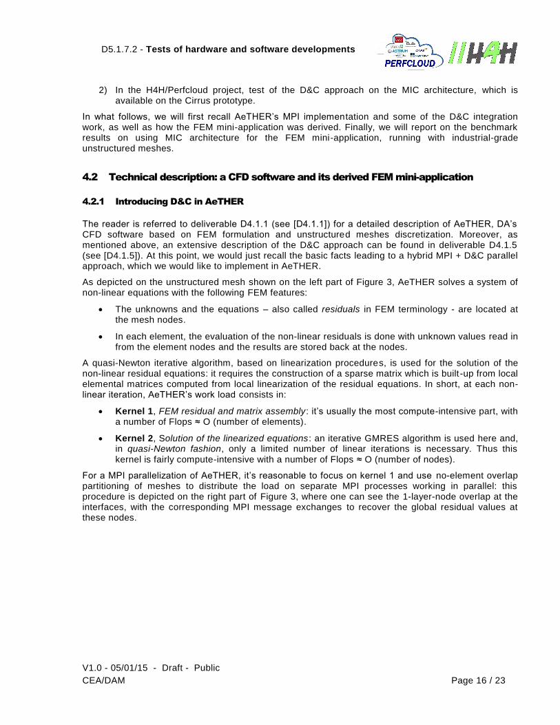
As depicted on the unstructured mesh shown on the left part of Figure 3, AeTHER solves a system of non-linear equations with the following FEM features:

The unknowns and the equations – also called residuals in FEM terminology - are located at the mesh nodes.

In each element, the evaluation of the non-linear residuals is done with unknown values read in from the element nodes and the results are stored back at the nodes.

A quasi-Newton iterative algorithm, based on linearization procedures, is used for the solution of the non-linear residual equations: it requires the construction of a sparse matrix which is built -up from local elemental matrices computed from local linearization of the residual equations. In short, at each non-linear iteration, AeTHER’s work load consists in:

Kernel 1, FEM residual and matrix assembly: it’s usually the most compute-intensive part, with a number of Flops ≈ O (number of elements).

Kernel 2, Solution of the linearized equations: an iterative GMRES algorithm is used here and, in quasi-Newton fashion, only a limited number of linear iterations is necessary. Thus this kernel is fairly compute-intensive with a number of Flops ≈ O (number of nodes).

For a MPI parallelization of AeTHER, it’s reasonable to focus on kernel 1 and use no-element overlap partitioning of meshes to distribute the load on separate MPI processes working in parallel: this procedure is depicted on the right part of Figure 3, where one can see the 1-layer-node overlap at the interfaces, with the corresponding MPI message exchanges to recover the global residual values at these nodes.


V1.0 - 05/01/15 - Draft - Public


F

i

g

u

r

e

E

r

r

o

r

!

M

a

i

n

D

o

c

u

m

e

n

t

O

n

l

y

.

Figure 3: MPI implementation via mesh partitioning. Left: sequential. Right: MPI.

To sum up, this MPI parallel implementation has the following features:

1) For kernel 1: the work load is very well balanced, as much as the mesh partitions are balanced in terms of number of elements.

2) For kernel 2: the work load is fairly balanced (when we compare 2 unstructured meshes, an equal number of elements does not guarantee an equal number of nodes…). Moreover there is a small overhead in terms of number of nodes, corresponding to the 1-layer-node overlap.

As one may suspect, this MPI-only (or flat MPI) model does not scale well when the number of physical cores (and corresponding MPI processes…) grows over the 500s. In addition to the growing complexity of the MPI messages and the sheer difficulty in process synchronization, the overhead in interfaces nodes for kernel 2 may become sizable: e.g. for an industrial -grade unstructured mesh of 7 Million-nodes, partitioned in 1024 mesh blocks, this overhead reaches 24% of the total number of nodes.

In DA, the above observations were made several years ago and since then, numerous efforts were done to keep a reasonable number of mesh blocks (and corresponding MPI processes) by introducing shared memory parallelism inside each MPI process, in short a hybrid MPI + threads model.

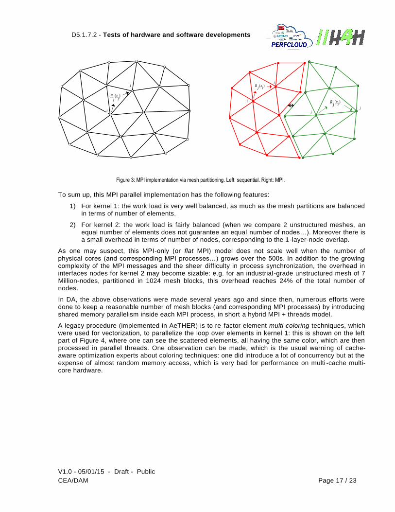
A legacy procedure (implemented in AeTHER) is to re-factor element multi-coloring techniques, which were used for vectorization, to parallelize the loop over elements in kernel 1: this is shown on the left part of Figure 4, where one can see the scattered elements, all having the same color, which are then processed in parallel threads. One observation can be made, which is the usual warning of cache-aware optimization experts about coloring techniques: one did introduce a lot of concurrency but at the expense of almost random memory access, which is very bad for performance on multi -cache multi-core hardware.

i

j

)(i

xj

Ri

j)(

ix

jR

)(i

xj

R

ij


V1.0 - 05/01/15 - Draft - Public


F

i

g

u

r

e

E

r

r

o

r

!

M

a

i

n

D

o

c

u

m

e

n

t

O

n

l

y

.

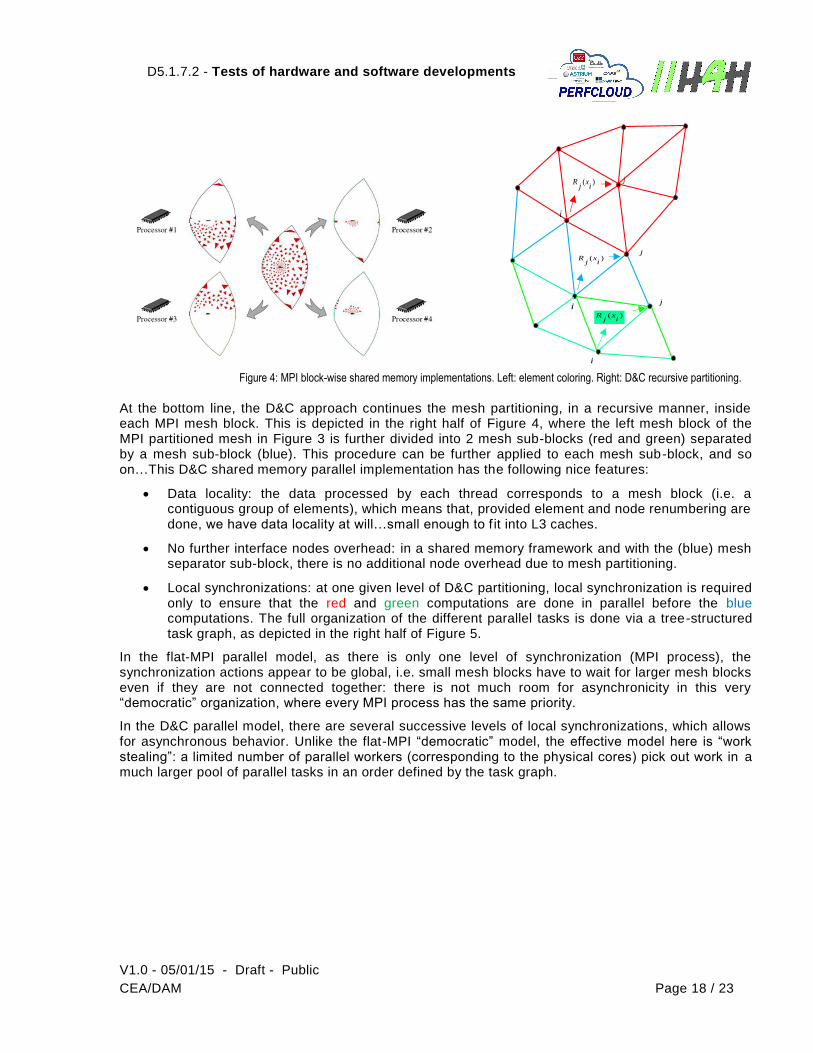
Figure 4: MPI block-wise shared memory implementations. Left: element coloring. Right: D&C recursive partitioning.

At the bottom line, the D&C approach continues the mesh partitioning, in a recursive manner, inside each MPI mesh block. This is depicted in the right half of Figure 4, where the left mesh block of the MPI partitioned mesh in Figure 3 is further divided into 2 mesh sub-blocks (red and green) separated by a mesh sub-block (blue). This procedure can be further applied to each mesh sub-block, and so on…This D&C shared memory parallel implementation has the following nice features:

Data locality: the data processed by each thread corresponds to a mesh block (i.e. a contiguous group of elements), which means that, provided element and node renumbering are done, we have data locality at will…small enough to f it into L3 caches.

No further interface nodes overhead: in a shared memory framework and with the (blue) mesh separator sub-block, there is no additional node overhead due to mesh partitioning.

Local synchronizations: at one given level of D&C partitioning, local synchronization is required only to ensure that the red and green computations are done in parallel before the blue computations. The full organization of the different parallel tasks is done via a tree-structured task graph, as depicted in the right half of Figure 5.

In the flat-MPI parallel model, as there is only one level of synchronization (MPI process), the synchronization actions appear to be global, i.e. small mesh blocks have to wait for larger mesh blocks even if they are not connected together: there is not much room for asynchronicity in this very “democratic” organization, where every MPI process has the same priority.

In the D&C parallel model, there are several successive levels of local synchronizations, which allows for asynchronous behavior. Unlike the flat-MPI “democratic” model, the effective model here is “work stealing”: a limited number of parallel workers (corresponding to the physical cores) pick out work in a much larger pool of parallel tasks in an order defined by the task graph.

i

j)(i

xj

R

)(i

xj

R

i

j

)(i

xj

Rj

i


V1.0 - 05/01/15 - Draft - Public


F

i

g

u

r

e

E

r

r

o

r

!

M

a

i

n

D

o

c

u

m

e

n

t

O

n

l

y

.

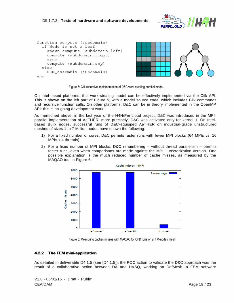
Figure 5: Cilk recursive implementation of D&C work stealing parallel model.

On Intel-based platforms, this work-stealing model can be effectively implemented via the Cilk API. This is shown on the left part of Figure 5, with a model source code, which includes Cilk commands and recursive function calls. On other platforms, D&C can be in theory implemented in the OpenMP API: this is on-going development work.

As mentioned above, in the last year of the H4H/Perfcloud project, D&C was introduced in the MPI-parallel implementation of AeTHER: more precisely, D&C was activated only for kernel 1. On Intel -based Bullx nodes, successful runs of D&C-equipped AeTHER on industrial-grade unstructured meshes of sizes 1 to 7 Million nodes have shown the following:

1) For a fixed number of cores, D&C permits faster runs with fewer MPI blocks (64 MPIs vs. 16 MPIs x 4 threads).

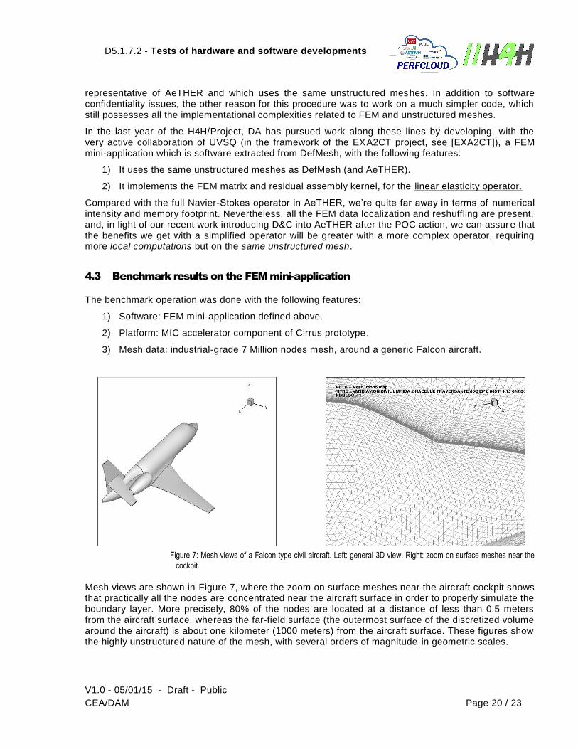
2) For a fixed number of MPI blocks, D&C renumbering – without thread parallelism – permits faster runs, even when comparisons are made against the MPI + vectorization version. One possible explanation is the much reduced number of cache misses, as measured by the MAQAO tool in Figure 6.

Figure 6: Measuring caches misses with MAQAO for CFD runs on a 1 M-nodes mesh

4.2.2 The FEM mini-application

As detailed in deliverable D4.1.5 (see [D4.1.5]), the POC action to validate the D&C approach was the result of a collaborative action between DA and UVSQ, working on DefMesh, a FEM software


V1.0 - 05/01/15 - Draft - Public


F

i

g

u

r

e

E

r

r

o

r

!

M

a

i

n

D

o

c

u

m

e

n

t

O

n

l

y

.

representative of AeTHER and which uses the same unstructured meshes. In addition to software confidentiality issues, the other reason for this procedure was to work on a much simpler code, which still possesses all the implementational complexities related to FEM and unstructured meshes.

In the last year of the H4H/Project, DA has pursued work along these lines by developing, with the very active collaboration of UVSQ (in the framework of the EXA2CT project, see [EXA2CT]), a FEM mini-application which is software extracted from DefMesh, with the following features:

1) It uses the same unstructured meshes as DefMesh (and AeTHER).

2) It implements the FEM matrix and residual assembly kernel, for the linear elasticity operator.

Compared with the full Navier-Stokes operator in AeTHER, we’re quite far away in terms of numerical intensity and memory footprint. Nevertheless, all the FEM data localization and reshuffling are present, and, in light of our recent work introducing D&C into AeTHER after the POC action, we can assur e that the benefits we get with a simplified operator will be greater with a more complex operator, requiring more local computations but on the same unstructured mesh.

4.3 Benchmark results on the FEM mini-application

The benchmark operation was done with the following features:

1) Software: FEM mini-application defined above.

2) Platform: MIC accelerator component of Cirrus prototype.

3) Mesh data: industrial-grade 7 Million nodes mesh, around a generic Falcon aircraft.

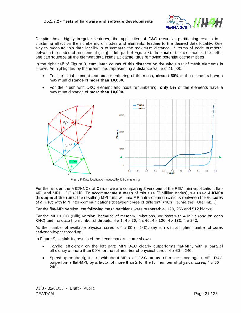
Figure 7: Mesh views of a Falcon type civil aircraft. Left: general 3D view. Right: zoom on surface meshes near the

cockpit.

Mesh views are shown in Figure 7, where the zoom on surface meshes near the aircraft cockpit shows that practically all the nodes are concentrated near the aircraft surface in order to properly simulate the boundary layer. More precisely, 80% of the nodes are located at a distance of less than 0.5 meters from the aircraft surface, whereas the far-field surface (the outermost surface of the discretized volume around the aircraft) is about one kilometer (1000 meters) from the aircraft surface. These figures show the highly unstructured nature of the mesh, with several orders of magnitude in geometric scales.


V1.0 - 05/01/15 - Draft - Public


F

i

g

u

r

e

E

r

r

o

r

!

M

a

i

n

D

o

c

u

m

e

n

t

O

n

l

y

.

Despite these highly irregular features, the application of D&C recursive partitioning results in a clustering effect on the numbering of nodes and elements, leading to the desired data locality. One way to measure this data locality is to compute the maximum distance, in terms of node numbers, between the nodes of an element (|i - j| in left part of Figure 8): the smaller this distance is, the better one can squeeze all the element data inside L3 cache, thus removing potential cache misses.

In the right half of Figure 8, cumulated counts of this distance on the whole set of mesh elements is shown. As highlighted by the green line, representing a distance value of 10,000:

For the initial element and node numbering of the mesh, almost 50% of the elements have a maximum distance of more than 10,000.

For the mesh with D&C element and node renumbering, only 5% of the elements have a maximum distance of more than 10,000.

Figure 8: Data localization induced by D&C clustering

For the runs on the MIC/KNCs of Cirrus, we are comparing 2 versions of the FEM mini -application: flat-MPI and MPI + DC (Cilk). To accommodate a mesh of this size (7 Million nodes), we used 4 KNCs throughout the runs: the resulting MPI runs will mix MPI intra-communications (between the 60 cores of a KNC) with MPI inter-communications (between cores of different KNCs, i.e. via the PCIe link…).

For the flat-MPI version, the following mesh partitions were prepared: 4, 128, 256 and 512 blocks.

For the MPI + DC (Cilk) version, because of memory limitations, we start with 4 MPIs (one on each KNC) and increase the number of threads: 4 x 1, 4 x 30, 4 x 60, 4 x 120, 4 x 180, 4 x 240.

As the number of available physical cores is 4 x 60 (= 240), any run with a higher number of cores activates hyper threading.

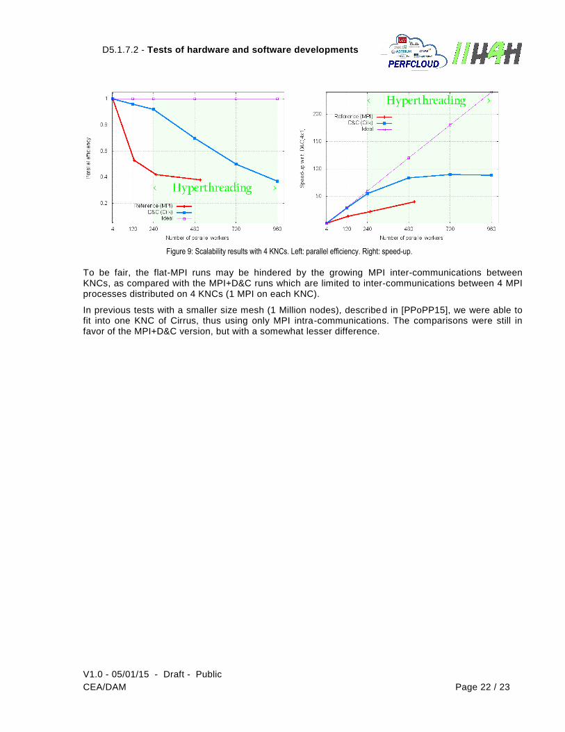
In Figure 9, scalability results of the benchmark runs are shown:

Parallel efficiency on the left part: MPI+D&C clearly outperforms flat-MPI, with a parallel efficiency of more than 90% for the full number of physical cores, 4 x 60 = 240.

Speed-up on the right part, with the 4 MPIs x 1 D&C run as reference: once again, MPI+D&C outperforms flat-MPI, by a factor of more than 2 for the full number of physical cores, 4 x 60 = 240.

i

j)(i

xj

R

)(i

xj

R

i

j

)(i

xj

Rj

i


V1.0 - 05/01/15 - Draft - Public


F

i

g

u

r

e

E

r

r

o

r

!

M

a

i

n

D

o

c

u

m

e

n

t

O

n

l

y

.

Figure 9: Scalability results with 4 KNCs. Left: parallel efficiency. Right: speed-up.

To be fair, the flat-MPI runs may be hindered by the growing MPI inter-communications between KNCs, as compared with the MPI+D&C runs which are limited to inter-communications between 4 MPI processes distributed on 4 KNCs (1 MPI on each KNC).

In previous tests with a smaller size mesh (1 Million nodes), described in [PPoPP15], we were able to fit into one KNC of Cirrus, thus using only MPI intra-communications. The comparisons were still in favor of the MPI+D&C version, but with a somewhat lesser difference.


V1.0 - 05/01/15 - Draft - Public


F

i

g

u

r

e

E

r

r

o

r

!

M

a

i

n

D

o

c

u

m

e

n

t

O

n

l

y

.

5 Abbreviations and acronyms

MIC®: Many Integrated Core. The public brand name is Intel Xeon Phi and describes processors having a lot of cores within its chip.

KNC: (Knights corner) Intel’s code name of the Xeon Phi.

#pragma simd: a directive provided by a programmer to tell the compiler to use special hardware functional units operating on a number of operands at the same time (SIMD stands for Single Instruction Multiple Data).

CFD: Computational Fluid Dynamics, for the numerical simulation of fluid flows.

FEM: Finite Element Method.

PCIe: PCI-eXpress, standard (Intel) solution to link CPU hardware with its many-core component (GPUs, MIC) on a node.

D&C: Divide and Conquer approach for shared memory parallelization. It has been successfully applied to the FEM matrix & residual assembly kernel, on fully unstructured 3D meshes.

GMRES: General Minimal RESidual. An effective (and popular) iterative algorithm for the solution of systems of sparse linear equations, with a general definite sparse matrix.

Cilk: An Intel API to implement shared memory thread parallelism. It’s particularly efficient for task-based parallelism.

6 References

[Github] https://github.com/HydroBench/Hydro.git [MAQAO] http://www.maqao.org/

[D4.1.1] F. CHALOT, Q.V. DINH, M. RAVACHOL, "Dassault Aviation - test cases description and requirements" H4H project, Deliverable D4.1.1, March 8, 2011.

[D4.1.5] F. CHALOT, Q.V. DINH, E. PETIT, L. THÉBAULT, "Dassault Aviation – final experimentation report" H4H project, Deliverable D4.1.5, September 27, 2013.

[EXA2CT] EXASCALE ALGORITHMS AND ADVANCED COMPUTATIONAL TECHNIQUES, European FP7 project, agreement no. 610741, September 2013 – September 2016. http://www.exa2ct.eu/

[PPOPP15] L. THÉBAULT, E. PETIT, Q.V. DINH, W. JALBY, "Scalable and efficient implementation of 3D unstructured meshes computations: a case study on Matrix Assembly”, accepted paper to PPoPP 2015, San Francisco, CA, USA, February 7-11, 2015.

https://github.com/HydroBench/Hydro.git

http://www.maqao.org/

Documents

Deliverable: D5.1.7.2 (L2.7.2) Tests of hardware and ... · PDF filethe OS installation as well as the network linking the nodes ... freefem++/3.16 lammps/7jun13 wrf/3.3 ... Tests