Embed Size (px)
Citation preview
Deliverable 3.6 “What-if Scenario Impact Studies based on real LV netw orks”
UoM-ENWL_LVNS_Deliverable3.6v14
9th Sep 2014
CONFIDENTIAL 1
Copyright © 2014 A. Navarro and L. Ochoa - The University of Manchester
Title: Deliverable 3.6 “What-if Scenario Impact
Studies based on real LV networks”
Synopsis: This report presents a Probabilistic Impact Assessment Methodology
for Low Carbon Technologies in real-life Low Voltage distribution feeders. This methodology has been applied on 128 real-life LV
feeder and the main results are summarised in this report.
Document ID:
Date:
Prepared for:
UoM-ENWL_LVNS_Deliverable3.6_v14
9
th September 2014
Rita Shaw Future Network Engineer Electricity North West Limited, UK
John Simpson LCN Tier 1 Project Manager
Electricity North West Limited, UK Dan Randles
Technology Development Manager Electricity North West Limited, UK
Prepared By: Alejandro Navarro Espinoza The University of Manchester Sackville Street, Manchester M13 9PL, UK
Supervised By: Dr Luis(Nando) Ochoa The University of Manchester
Sackville Street, Manchester M13 9PL, UK
Contacts: Alejandro Navarro Espinosa

Deliverable 3.6 “What-if Scenario Impact Studies based on real LV netw orks”
UoM-ENWL_LVNS_Deliverable3.6v14
9th Sep 2014
CONFIDENTIAL 2
Copyright © 2014 A. Navarro and L. Ochoa - The University of Manchester
Executive Summary This document corresponds to Deliverable 3.6 “What-if Scenario Impact Studies based on real LV networks”. This report is part of the Low Carbon Network Fund Tier 1 project “LV Network Solutions” run by Electricity North West Limited (ENWL), the Distribution Network Operator of the North West of
England, and The University of Manchester.
In particular, this report studies and assesses the impacts of low carbon technologies (LCT) in real-life LV distribution feeders. This entails analysing the capabilities of these networks to host new LCT
studying the penetration levels (% of houses with the technology) that trigger technical problems.
The increase of LCT in LV networks could produce voltage issues (drop and/or rise), thermal overload of the lines or transformers, and higher energy losses. To assess the extent of these effects on the
performance of LV networks, a Probabilistic Impact Assessment Methodology is implemented in this report. This methodology combines real networks, time-series analysis, a Monte Carlo approach (hundreds of simulations per penetration level) for loads and LCT (behaviour, location and size), and
the use of an unbalance power flow engine to assess the impacts. Several metrics are used to assess the corresponding impacts. This includes percentage of customers with voltage problems per feeder, utilization level of the feeder, daily energy losses, probability distribution of having certain number of
customers with problems, etc. With this methodology, the Distribution Network Operator can analyse the potential risk (in terms of probabilities) of having a given LCT penetration in their networks.
The inputs for the Probabilistic Impact Assessment Methodology are the loads and LCT profiles, and
the real-life LV networks. Hence, the creation of time-series profiles for loads, photovoltaic panels, electric vehicles, electric heat pumps and micro combined heat and power are also presented. The studies were carried out on 128 feeders implemented in OpenDSS (power flow engine) from the GIS
data provided by ENWL, analysing the effects of residential photovoltaic panels (PV), electric heat pumps (EHP), electric vehicles (EV) and micro combined heat and power units (µCHP).
Based on the application of the proposed probabilistic methodology, the following (general)
conclusions can be made:
Low Carbon Technologies
o The percentage of feeders with voltage problems is higher in the PV case (about 64%
of the feeders) and the percentage of feeders with thermal problems is higher in the EHP case (around 57% of the feeders).
o In the PV case, the first occurrence of problems is driven by voltage issues in all the
feeders examined. For the EHP and EV case, the first occurrence of problems is driven by voltage and also by thermal issues. Indeed, the 45% and 35% of the feeders have the first problem due to thermal issues in the EHP and EV case, respectively.
Occurrence of Problems
o Feeders with less than 25 customers do not present any problems among the feeders analysed.
o The best individual metrics for the LCT analysed to explain the occurrence of
problems in LV feeders are: the Initial Utilization Level and the Total Path Impedance.
o The combination of the Initial Utilization Level and the Total Path Impedance increases the coefficient of determination (correlation performance) for all the
technologies. In fact, the multiplication of these two metrics produces a coefficient of determination equals to 0.80, 0.88 and 0.79 for the PV, EHP and EV cases, respectively.
Monitoring. The utilization of low resolution data (e.g., 15 min, 30 min and 60 min) for loads and generation profiles underestimates the impacts of LCT in LV networks.
Network Modelling. The utilization of single-phase (balanced) network and load
representations underestimates the impacts of LCT in LV networks.

Deliverable 3.6 “What-if Scenario Impact Studies based on real LV netw orks”
UoM-ENWL_LVNS_Deliverable3.6v14
9th Sep 2014
CONFIDENTIAL 3
Copyright © 2014 A. Navarro and L. Ochoa - The University of Manchester
Contents Contents ...................................................................................................................................... 3
1 Introduction ............................................................................................................... 4
1.1 Report Structure .......................................................................................................... 4
2 Profiling of Low Carbon Technologies ...................................................................... 5
2.1 Load Profiles ............................................................................................................... 5
2.2 Photovoltaic Profiles .................................................................................................... 5
2.3 Micro Combined Heat and Power ................................................................................. 7
2.4 Electric heat pump profiles ........................................................................................... 8
2.5 Electric Vehicles Profiles .............................................................................................. 9
2.6 Aggregated Profiles – Diversified Profiles .....................................................................11 2.6.1 Sensitivities for the EV ................................................................................................13
3 LV Networks .............................................................................................................16
3.1 Modelling Summary ....................................................................................................16
3.2 Studied LV Networks ..................................................................................................16
4 Probabilistic Impact Assessment Methodology .......................................................21
4.1 Literature Review .......................................................................................................21
4.2 Methodology ..............................................................................................................21
4.3 Assessment Metrics....................................................................................................22 4.3.1 Voltage Problems .......................................................................................................23 4.3.2 Thermal Problems ......................................................................................................24 4.3.3 Energy Losses ...........................................................................................................25 4.3.4 Probability Distribution of Impacts ................................................................................26 4.3.5 Additional Metric for DG Technologies .........................................................................28
4.4 Case studies ..............................................................................................................30 4.4.1 Balanced versus unbalanced LV feeder .......................................................................30 4.4.2 Analysis of data granularity .........................................................................................31 4.4.3 Utilization of ELEXON profiles .....................................................................................32 4.4.4 EV Sensitivities: Fast charging and Peak shifting ..........................................................35 4.4.5 Additional Feeder Assessment ....................................................................................36
5 Multi-Feeder Analysis ...............................................................................................39
5.1 Results Overview .......................................................................................................39 5.1.1 General Analysis ........................................................................................................39 5.1.2 Occurrence of the First Problems ................................................................................41 5.1.3 Transformer thermal ratings ........................................................................................43
5.2 Metrics and Correlations .............................................................................................45 5.2.1 Metrics.......................................................................................................................45 5.2.2 Correlation Analysis....................................................................................................46 5.2.3 LCT Correlation Analysis ............................................................................................49
6 Conclusions .............................................................................................................58
7 References ...............................................................................................................60
Deliverable 3.6 “What-if Scenario Impact Studies based on real LV netw orks”
UoM-ENWL_LVNS_Deliverable3.6v14
9th Sep 2014
CONFIDENTIAL 4
Copyright © 2014 A. Navarro and L. Ochoa - The University of Manchester
1 Introduction As part of the transition towards a low carbon economy, Electricity North West Limited (ENWL), the Distribution Network Operator of the North West of England, is involved in different projects funded by the Low Carbon Network Fund. The University of Manchester is part of several of those projects. In
particular, this report is part of the Tier 1 project called “LV Networks Solutions”.
Penetrations of low carbon technologies such as photovoltaic panels, electric vehicles, micro combined heat and power and heat pumps (called hereinafter Low Carbon Technologies or LCT), are
likely to increase in the future, particularly at low voltage (LV) networks. The lack of observability and network modelling, typical of this voltage level, are the major barriers to assess how capable are these networks to cope with the future.
By modelling and analysing real-life LV networks, this project assesses the impacts of LCT and the technical viability of innovative solutions to manage future networks . Thus, the main objective is to provide greater understanding of the characteristics, behaviour, and future needs of LV networks.
Particularly, in this report the impacts of LCT in LV distribution networks are analysed in detail. In fact, hundreds of computer-based models for LV feeders are created using the state-of-the-art distribution analysis software package OpenDSS developed by EPRI (Electric Power Research Institute, USA). To
populate these feeders, thousands of individual profiles are created for loads, photovoltaic panels, electric vehicles, electric heat pump and micro combined heat and power. The methodology to create these profiles and their individual and aggregated behaviours are presented in this report.
To assess the extent of the LCT effects on the performance of LV networks, a Probabilistic Impact Assessment Methodology is implemented. This methodology embeds the uncertainties related to LCT such as, location, size, behaviour, etc., and considers different penetration levels (percentage of
houses with the new technology). Penetration levels ranging from 0% to 100% with increments of 10% are developed. This analysis takes into account 5-minute resolution time-series profiles and adopts a realistic representation of the unbalanced nature of LV networks (using OpenDSS). Thus, for each
penetration level, a random siting of loads and LCT profiles (following a realistic probability distribution) is carried out to then run a power flow in order to capture the main results. This process is repeated one hundred times for each penetration level and is developed for each LCT independently.
The results from the Probabilistic Impact Assessment Methodology are analysed through several metrics. In this report, the percentage of customers with voltage problems, the utilization level (according to the rating capacity) of the head of the feeder, the daily energy losses , and the
cumulative probability distribution of having problems are adopted and presented.
The application of this probabilistic methodology considering several case studies is illustrated through the analysis of two particular feeders (Whitchurch road, feeder feature number: 528267202 and Mellor
Street, feeder feature number: 227045574). This analysis is then extended to the 128 LV feeders considering all LCT. This allows investigating the main characteristics of LV feeders (e.g., number of customers, length, etc.) that could be related to the occurrence of thermal and/or voltage problems.
Thus, by understanding this relationship it is possible to produce general guidelines in terms of the LCT penetration level that results in technical issues.
1.1 Report Structure
The rest of this report is divided into six chapters. Chapter 2 presents a brief summary about the individual profiles created in this project, namely, loads, electric vehicles, photovoltaic panels, electric
heat pumps and micro combine heat and power units. The methodology to create them is also presented in this chapter. The aggregated behaviour of 100 of these profiles is also presented. The modelling of the studied LV networks is presented in Chapter 3. The Probabilistic Impact Assessment
methodology is explained in Chapter 4; there the methodology, assessment metrics and the case studies are presented. The application of this methodology on 128 feeders is carried out in Chapter 5; the results of this analysis are also presented in this chapter for all the LCT under analysis. The
conclusions are drawn in Chapter 6. Finally, the main references are presented in Chapter 7.
Deliverable 3.6 “What-if Scenario Impact Studies based on real LV netw orks”
UoM-ENWL_LVNS_Deliverable3.6v14
9th Sep 2014
CONFIDENTIAL 5
Copyright © 2014 A. Navarro and L. Ochoa - The University of Manchester
2 Profiling of Low Carbon Technologies To understand the impacts of LCT on low voltage distribution networks, the creation of realistic time-series profiles is fundamental. In this section, a summary of the main characteristic of the profiles used/created is presented. Further details are included in the Deliverable 3.5 “Creation of aggregated
profiles with and without new loads and DER based on monitored data” [1]. In particular, these profiles correspond to un-restricted residential loads, photovoltaic panels (PV), micro-combined heat and power (µCHP), electric heat pumps (EHP) and electric vehicles (EV). All the profiles produced for the
studies presented in this report consider 5-minute resolution data. This is to reduce the simulation time but it does not compromise accuracy.
2.1 Load Profiles
The load profiles are obtained from the computational model developed by CREST (Centre for Renewable Energy Systems Technology) at Loughborough University. This model creates time-series
profiles for residential loads based on the domestic behaviour of British costumers [2]; it takes into account the number of people at home, the type of day, the month, and the uses of the appliances. In this way, it is possible to have one minute resolution profiles, indicating which appliance is ON and
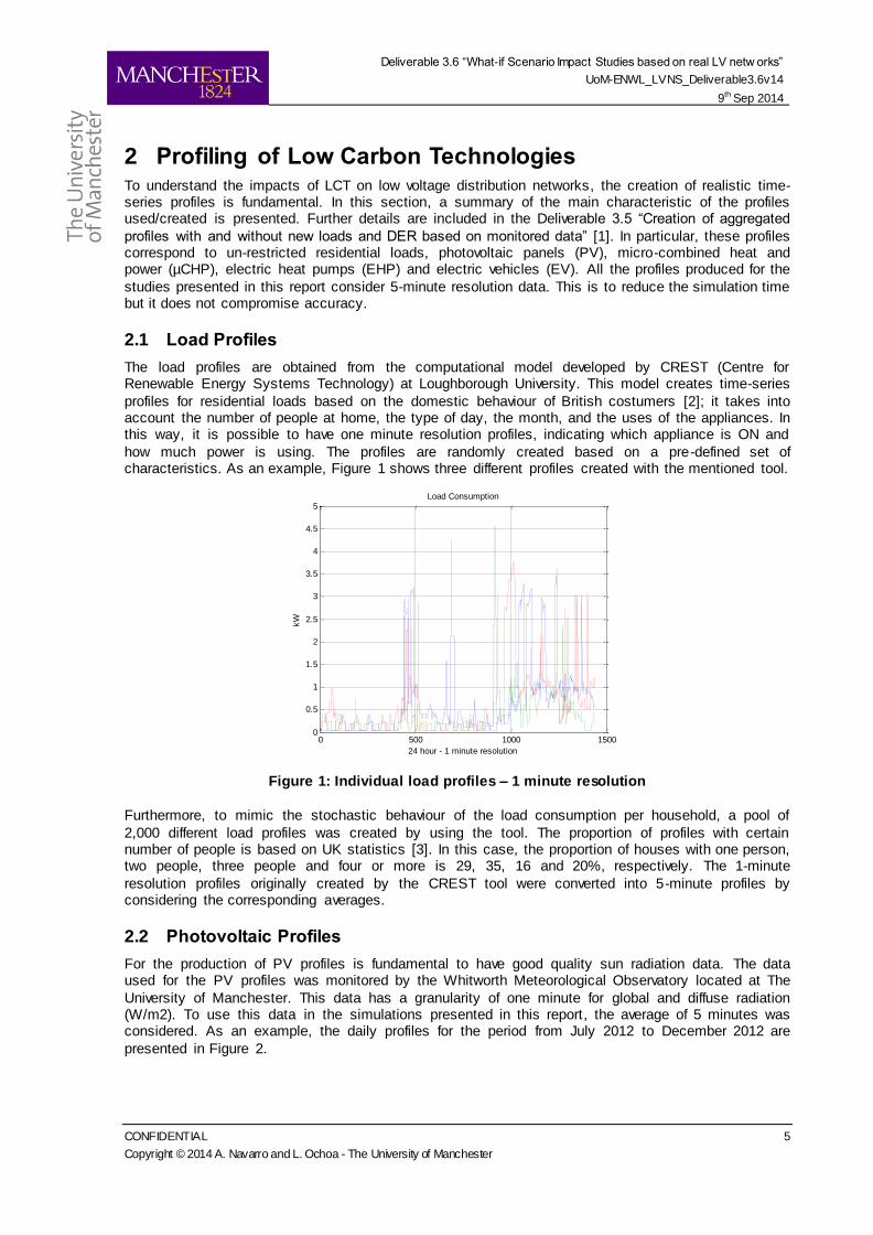
how much power is using. The profiles are randomly created based on a pre-defined set of characteristics. As an example, Figure 1 shows three different profiles created with the mentioned tool.
Figure 1: Individual load profiles – 1 minute resolution
Furthermore, to mimic the stochastic behaviour of the load consumption per household, a pool of
2,000 different load profiles was created by using the tool. The proportion of profiles with certain number of people is based on UK statistics [3]. In this case, the proportion of houses with one person, two people, three people and four or more is 29, 35, 16 and 20%, respectively. The 1-minute
resolution profiles originally created by the CREST tool were converted into 5-minute profiles by considering the corresponding averages.
2.2 Photovoltaic Profiles
For the production of PV profiles is fundamental to have good quality sun radiation data. The data used for the PV profiles was monitored by the Whitworth Meteorological Observatory located at The
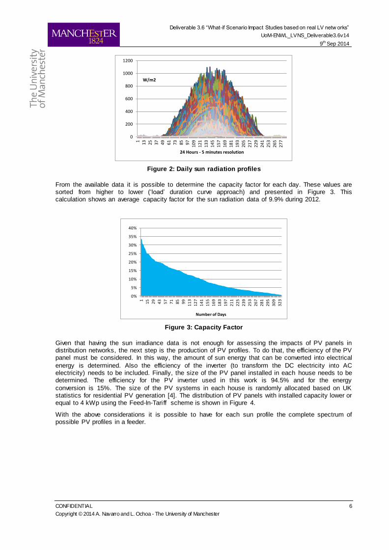
University of Manchester. This data has a granularity of one minute for global and diffuse radiation (W/m2). To use this data in the simulations presented in this report, the average of 5 minutes was considered. As an example, the daily profiles for the period from July 2012 to December 2012 are
presented in Figure 2.
0 500 1000 15000
0.5
1
1.5
2
2.5
3
3.5
4
4.5
5
24 hour - 1 minute resolution
kW
Load Consumption
Deliverable 3.6 “What-if Scenario Impact Studies based on real LV netw orks”
UoM-ENWL_LVNS_Deliverable3.6v14
9th Sep 2014
CONFIDENTIAL 6
Copyright © 2014 A. Navarro and L. Ochoa - The University of Manchester
Figure 2: Daily sun radiation profiles
From the available data it is possible to determine the capacity factor for each day. These values are sorted from higher to lower (‘load’ duration curve approach) and presented in Figure 3. This calculation shows an average capacity factor for the sun radiation data of 9.9% during 2012.
Figure 3: Capacity Factor
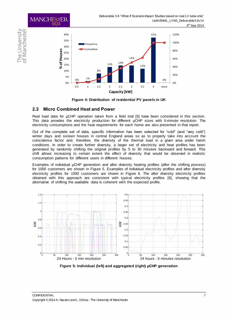
Given that having the sun irradiance data is not enough for assessing the impacts of PV panels in distribution networks, the next step is the production of PV profiles. To do that, the efficiency of the PV panel must be considered. In this way, the amount of sun energy that can be converted into electrical
energy is determined. Also the efficiency of the inverter (to transform the DC electricity into AC electricity) needs to be included. Finally, the size of the PV panel installed in each house needs to be determined. The efficiency for the PV inverter used in this work is 94.5% and for the energy
conversion is 15%. The size of the PV systems in each house is randomly allocated based on UK statistics for residential PV generation [4]. The distribution of PV panels with installed capacity lower or equal to 4 kWp using the Feed-In-Tariff scheme is shown in Figure 4.
With the above considerations it is possible to have for each sun profile the complete spectrum of possible PV profiles in a feeder.
0
200
400
600
800
1000
1200
1
13
25
37
49
61
73
85
97
10
9
12
1
13
3
14
5
15
7
16
9
18
1
19
3
20
5
21
7
22
9
24
1
25
3
26
5
27
7
W/m2
24 Hours - 5 minutes resolution
0%
5%
10%
15%
20%
25%
30%
35%
40%
1
15
29
43
57
71
85
99
11
3
12
7
14
1
15
5
16
9
18
3
19
7
21
1
22
5
23
9
25
3
26
7
28
1
29
5
30
9
32
3
Number of Days
Deliverable 3.6 “What-if Scenario Impact Studies based on real LV netw orks”
UoM-ENWL_LVNS_Deliverable3.6v14
9th Sep 2014
CONFIDENTIAL 7
Copyright © 2014 A. Navarro and L. Ochoa - The University of Manchester
Figure 4: Distribution of residential PV panels in UK
2.3 Micro Combined Heat and Power
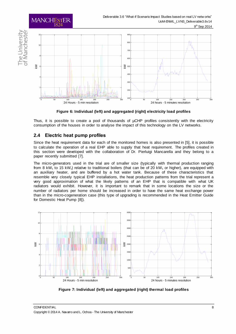
Real load data for µCHP operation taken from a field trial [5] have been considered in this section. This data provides the electricity production for different µCHP sizes with 5-minute resolution. The electricity consumptions and the heat requirements for each home are also presented in that report.
Out of the complete set of data, specific information has been selected for “cold” (and “very cold”) winter days and sixteen houses in central England areas so as to properly take into account the coincidence factor and, therefore, the diversity of the thermal load in a given area under harsh
conditions. In order to create further diversity, a larger set of electricity and heat profiles has been generated by randomly shifting the original profiles by 5 to 30 minutes backward and forward. This shift allows increasing to certain extent the effect of diversity that would be observed in realistic
consumption patterns for different users in different houses.
Examples of individual µCHP generation and after diversity heating profiles (after the shifting process) for 1000 customers are shown in Figure 5. Examples of individual electricity profiles and after diversity
electricity profiles for 1000 customers are shown in Figure 6. The after diversity electricity profiles obtained with this approach are consistent with typical electricity profiles [6], showing that the alternative of shifting the available data is coherent with the expected profile.
Figure 5: Individual (left) and aggregated (right) µCHP generation
0%1%
8%
13%14%
14%
12%
37%
0%0%
20%
40%
60%
80%
100%
120%
0%
5%
10%
15%
20%
25%
30%
35%
40%
0.5 1 1.5 2 2.5 3 3.5 4 more
% o
f H
ou
ses
Capacity [kW]
Frequency
Cumulative
0 50 100 150 200 250 3000
0.2
0.4
0.6
0.8
1
1.2
1.4
kW
24 Hours - 5 min resolution0 50 100 150 200 250 300
0
0.05
0.1
0.15
0.2
0.25
0.3
0.35
0.4
0.45
0.5
24 hours - 5 minutes resolution
kW
Deliverable 3.6 “What-if Scenario Impact Studies based on real LV netw orks”
UoM-ENWL_LVNS_Deliverable3.6v14
9th Sep 2014
CONFIDENTIAL 8
Copyright © 2014 A. Navarro and L. Ochoa - The University of Manchester
Figure 6: Individual (left) and aggregated (right) electricity load profiles
Thus, it is possible to create a pool of thousands of µCHP profiles consistently with the electricity consumption of the houses in order to analyse the impact of this technology on the LV networks.
2.4 Electric heat pump profiles
Since the heat requirement data for each of the monitored homes is also presented in [5], it is possible
to calculate the operation of a real EHP able to supply that heat requirement. The profiles created in this section were developed with the collaboration of Dr. Pierluigi Mancarella and they belong to a paper recently submitted [7].
The micro-generators used in the trial are of smaller size (typically with thermal production ranging from 8 kW t to 15 kW t) relative to traditional boilers (that can be of 20 kW t or higher), are equipped with an auxiliary heater, and are buffered by a hot water tank. Because of these characteristics that
resemble very closely typical EHP installations, the heat production patterns from the trial represent a very good approximation of what the likely patterns of an EHP that is compatible with what UK radiators would exhibit. However, it is important to remark that in some locations the size or the
number of radiators per home should be increased in order to have the same heat exchange power than in the micro-cogeneration case (this type of upgrading is recommended in the Heat Emitter Guide for Domestic Heat Pump [8]).
Figure 7: Individual (left) and aggregated (right) thermal load profiles
0 50 100 150 200 250 3000
2
4
6
8
10
12kW
24 Hours - 5 min resolution0 50 100 150 200 250 300
100
200
300
400
500
600
700
800
900
24 hours - 5 minutes resolution
kW
0 50 100 150 200 250 3000
2
4
6
8
10
12
kW
24 Hours - 5 min resolution0 50 100 150 200 250 300
0
500
1000
1500
2000
2500
3000
3500
4000
24 hours - 5 minutes resolution
kW
Deliverable 3.6 “What-if Scenario Impact Studies based on real LV netw orks”
UoM-ENWL_LVNS_Deliverable3.6v14
9th Sep 2014
CONFIDENTIAL 9
Copyright © 2014 A. Navarro and L. Ochoa - The University of Manchester
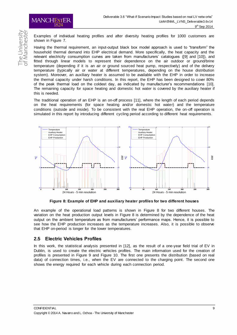
Examples of individual heating profiles and after diversity heating profiles for 1000 customers are shown in Figure 7.
Having the thermal requirement, an input-output black box model approach is used to “transform” the
household thermal demand into EHP electrical demand. More specifically, the heat capacity and the relevant electricity consumption curves are taken from manufacturers’ catalogues ([9] and [10]), and fitted through linear models to represent their dependence on the air outdoor or ground/brine
temperature (depending if it is an air or ground sourced heat pump, respectively) and of the delivery temperature (typically air or water at different temperatures, depending on the house distribution system). Moreover, an auxiliary heater is assumed to be available with the EHP in order to increase
the thermal capacity under harsh conditions. In this report, the EHP has been designed to cover 80% of the peak thermal load on the coldest day, as indicated by manufacturer’s recommendations [10]. The remaining capacity for space heating and domestic hot water is covered by the auxiliary heater if
this is needed.
The traditional operation of an EHP is an on-off process [11], where the length of each period depends on the heat requirements (for space heating and/or domestic hot water) and the temperature
conditions (outside and inside). To be consistent with the real EHP operation, the on-off operation is simulated in this report by introducing different cycling period according to different heat requirements.
Figure 8: Example of EHP and auxiliary heater profiles for two different houses
An example of the operational load patterns is shown in Figure 8 for two different houses. The variation on the heat production output levels in Figure 8 is determined by the dependence of the heat
output on the ambient temperature as from manufacturers’ performance maps. Hence, it is possible to see how the EHP production increases as the temperature increases. Also, it is possible to observe that EHP on-period is longer for the lower temperatures.
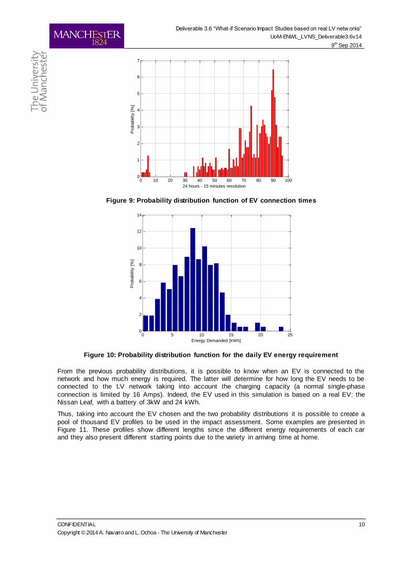
2.5 Electric Vehicles Profiles
In this work, the statistical analysis presented in [12], as the result of a one-year field trial of EV in
Dublin, is used to create the electric vehicles profiles. The main information used for the creation of profiles is presented in Figure 9 and Figure 10. The first one presents the distribution (based on real data) of connection times, i.e., when the EV are connected to the charging point. The second one
shows the energy required for each vehicle during each connection period.
0 50 100 150 200 250 300-5
0
5
10
ºC
24 Hours - 5 min resolution
0 50 100 150 200 250 3000
5
10
15
kW
Temperature
Auxiliary Heater
EHP Consumption
EHP Production
0 50 100 150 200 250 300-5
0
5
10ºC
24 Hours - 5 min resolution
0 50 100 150 200 250 3000
5
10
15
kW
Temperature
Auxiliary Heater
EHP Consumption
EHP Production
Deliverable 3.6 “What-if Scenario Impact Studies based on real LV netw orks”
UoM-ENWL_LVNS_Deliverable3.6v14
9th Sep 2014
CONFIDENTIAL 10
Copyright © 2014 A. Navarro and L. Ochoa - The University of Manchester
Figure 9: Probability distribution function of EV connection times
Figure 10: Probability distribution function for the daily EV energy requirement
From the previous probability distributions, it is possible to know when an EV is connected to the network and how much energy is required. The latter will determine for how long the EV needs to be connected to the LV network taking into account the charging capacity (a normal single-phase
connection is limited by 16 Amps). Indeed, the EV used in this simulation is based on a real EV: the Nissan Leaf, with a battery of 3kW and 24 kWh.
Thus, taking into account the EV chosen and the two probability distributions it is possible to create a
pool of thousand EV profiles to be used in the impact assessment. Some examples are presented in Figure 11. These profiles show different lengths since the different energy requirements of each car and they also present different starting points due to the variety in arriving time at home.
0 10 20 30 40 50 60 70 80 90 1000
1
2
3
4
5
6
7
24 hours - 15 minutes resolution
Pro
babili
ty [
%]
0 5 10 15 20 250
2
4
6
8
10
12
14
Energy Demanded [kWh]
Pro
babili
ty [
%]
Deliverable 3.6 “What-if Scenario Impact Studies based on real LV netw orks”
UoM-ENWL_LVNS_Deliverable3.6v14
9th Sep 2014
CONFIDENTIAL 11
Copyright © 2014 A. Navarro and L. Ochoa - The University of Manchester
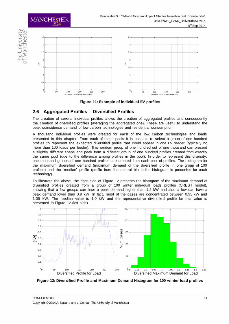
Figure 11: Example of individual EV profiles
2.6 Aggregated Profiles – Diversified Profiles
The creation of several individual profiles allows the creation of aggregated profiles and consequently
the creation of diversified profiles (averaging the aggregated one). These are useful to understand the peak coincidence demand of low carbon technologies and residential consumption.
A thousand individual profiles were created for each of the low carbon technologies and loads
presented in this chapter. From each of these pools it is possible to select a group of one hundred profiles to represent the expected diversified profile that could appear in one LV feeder (typically no more than 100 loads per feeder). This random group of one hundred out of one thousand can present
a slightly different shape and peak from a different group of one hundred profiles created from exactly the same pool (due to the difference among profiles in the pool). In order to represent this diversity, one thousand groups of one hundred profiles are created from each pool of profiles. The histogram for
the maximum diversified demand (maximum demand of the diversified profile in one group of 100 profiles) and the “median” profile (profile from the central bin in the histogram is presented for each technology).
To illustrate the above, the right side of Figure 12 presents the histogram of the maximum demand of diversified profiles created from a group of 100 winter individual loads profiles (CREST model), showing that a few groups can have a peak demand higher than 1.2 kW and also a few can have a
peak demand lower than 0.9 kW. In fact, most of the cases are concentrated between 0.95 kW and 1.05 kW. The median value is 1.0 kW and the representative diversified profile for this value is presented in Figure 12 (left side).
Figure 12: Diversified Profile and Maximum Demand Histogram for 100 winter load profiles
0 50 100 150 200 2500
0.5
1
1.5
2
2.5
3
3.5
24 hours - 5 minutes resolution
kW
0 50 100 150 200 2500
0.5
1
1.5
2
2.5
3
3.5
24 hours - 5 minutes resolution
kW
0 50 100 150 200 250 3000
0.1
0.2
0.3
0.4
0.5
0.6
0.7
0.8
0.9
1
Diversified Profile for Load
[kW
]
0.8 0.85 0.9 0.95 1 1.05 1.1 1.15 1.2 1.250
50
100
150
200
250
Diversified Maximum Demand for Load
Nu
m C
ase
s
Deliverable 3.6 “What-if Scenario Impact Studies based on real LV netw orks”
UoM-ENWL_LVNS_Deliverable3.6v14
9th Sep 2014
CONFIDENTIAL 12
Copyright © 2014 A. Navarro and L. Ochoa - The University of Manchester
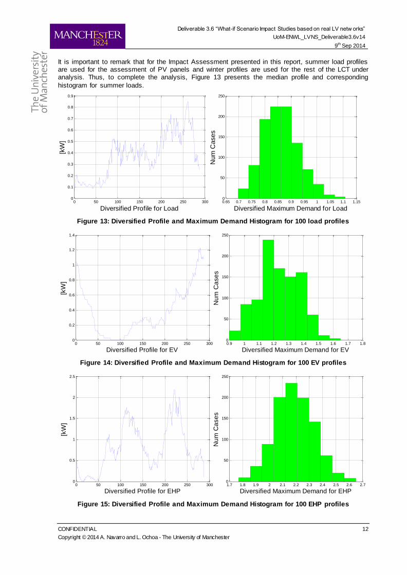
It is important to remark that for the Impact Assessment presented in this report, summer load profiles are used for the assessment of PV panels and winter profiles are used for the rest of the LCT under analysis. Thus, to complete the analysis, Figure 13 presents the median profile and corresponding
histogram for summer loads.
Figure 13: Diversified Profile and Maximum Demand Histogram for 100 load profiles
Figure 14: Diversified Profile and Maximum Demand Histogram for 100 EV profiles
Figure 15: Diversified Profile and Maximum Demand Histogram for 100 EHP profiles
0 50 100 150 200 250 3000
0.1
0.2
0.3
0.4
0.5
0.6
0.7
0.8
0.9
Diversified Profile for Load
[kW
]
0.65 0.7 0.75 0.8 0.85 0.9 0.95 1 1.05 1.1 1.150
50
100
150
200
250
Diversified Maximum Demand for LoadN
um
Cases
0 50 100 150 200 250 3000
0.2
0.4
0.6
0.8
1
1.2
1.4
Diversified Profile for EV
[kW
]
0.9 1 1.1 1.2 1.3 1.4 1.5 1.6 1.7 1.80
50
100
150
200
250
Diversified Maximum Demand for EV
Nu
m C
ase
s
0 50 100 150 200 250 3000
0.5
1
1.5
2
2.5
Diversified Profile for EHP
[kW
]
1.7 1.8 1.9 2 2.1 2.2 2.3 2.4 2.5 2.6 2.70
50
100
150
200
250
Diversified Maximum Demand for EHP
Nu
m C
ase
s
Deliverable 3.6 “What-if Scenario Impact Studies based on real LV netw orks”
UoM-ENWL_LVNS_Deliverable3.6v14
9th Sep 2014
CONFIDENTIAL 13
Copyright © 2014 A. Navarro and L. Ochoa - The University of Manchester
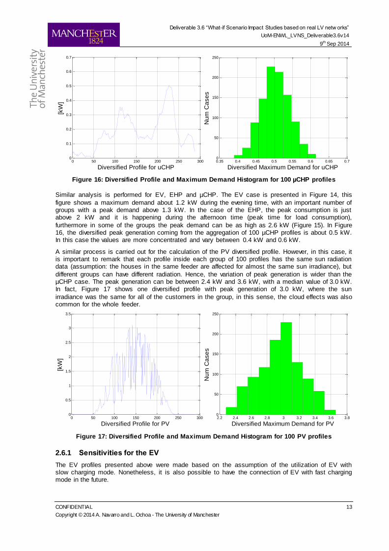
Figure 16: Diversified Profile and Maximum Demand Histogram for 100 µCHP profiles
Similar analysis is performed for EV, EHP and µCHP. The EV case is presented in Figure 14, this
figure shows a maximum demand about 1.2 kW during the evening time, with an important number of groups with a peak demand above 1.3 kW. In the case of the EHP, the peak consumption is just above 2 kW and it is happening during the afternoon time (peak time for load consumption),
furthermore in some of the groups the peak demand can be as high as 2.6 kW (Figure 15). In Figure 16, the diversified peak generation coming from the aggregation of 100 µCHP profiles is about 0.5 kW. In this case the values are more concentrated and vary between 0.4 kW and 0.6 kW.
A similar process is carried out for the calculation of the PV diversified profile. However, in this case, it is important to remark that each profile inside each group of 100 profiles has the same sun radiation data (assumption: the houses in the same feeder are affected for almost the same sun irradiance), but
different groups can have different radiation. Hence, the variation of peak generation is wider than the µCHP case. The peak generation can be between 2.4 kW and 3.6 kW, with a median value of 3.0 kW. In fact, Figure 17 shows one diversified profile with peak generation of 3.0 kW, where the sun
irradiance was the same for all of the customers in the group, in this sense, the cloud effects was also common for the whole feeder.
Figure 17: Diversified Profile and Maximum Demand Histogram for 100 PV profiles
2.6.1 Sensitivities for the EV
The EV profiles presented above were made based on the assumption of the utilization of EV with slow charging mode. Nonetheless, it is also possible to have the connection of EV with fast charging mode in the future.
0 50 100 150 200 250 3000
0.1
0.2
0.3
0.4
0.5
0.6
0.7
Diversified Profile for uCHP
[kW
]
0.35 0.4 0.45 0.5 0.55 0.6 0.65 0.70
50
100
150
200
250
Diversified Maximum Demand for uCHP
Nu
m C
ase
s
0 50 100 150 200 250 3000
0.5
1
1.5
2
2.5
3
3.5
Diversified Profile for PV
[kW
]
2.2 2.4 2.6 2.8 3 3.2 3.4 3.6 3.80
50
100
150
200
250
Diversified Maximum Demand for PV
Nu
m C
ase
s

Deliverable 3.6 “What-if Scenario Impact Studies based on real LV netw orks”
UoM-ENWL_LVNS_Deliverable3.6v14
9th Sep 2014
CONFIDENTIAL 14
Copyright © 2014 A. Navarro and L. Ochoa - The University of Manchester
Figure 18: Diversified Profile and Maximum Demand Histogram for 100 Fast Charging EV profiles
To analyse this effect, the same procedure considered in Section 2.5 is repeated but this time using an EV with a rating capacity of 6 kW (twice than in the slow mode) and an energy capacity of 24 kWh (same battery as in the slow mode). With this higher demand, the individual power requirements from
the grid will be higher and the time of connection will be lower, hence reducing the coincidence among different EV. These two effects will determine the diversified peak demand for the fast charging EV.
Again, a pool of 1000 fast charging EV profiles were created, and 1000 sets of 100 profiles were
analysed. The main results are presented in Figure 18, indicating a peak demand during the night time about 1.5 kW and presenting several scenarios with a peak demand between 1.5 kW and 2.0 kW. In comparison with the slow charging mode (Figure 14), the median value of peak demand is 25% higher
in the fast charging mode, although the rating capacity is 100% larger.
An important point in the analysis implemented is that the probability distributions for “connection time” and “energy required in each EV connection” are coming from real information gathered in Ireland and
therefore they will not necessarily represent the behaviour of customers in the North West of England. In order to incorporate the possibility to have the peak requirement of EV during the afternoon peak in England (so called tea time peak) instead of having the peak at 21:00 as in the Irish real data, the
“connection time” curve was shifted accordingly and the new results are presented in Figure 19 for the slow mode case (base EV case). In this new case, the peak diversified demand is also 1.2 kW in comparison with the case without shifting, but now the peak occurs at 19:00.
Figure 19: Diversified Profile and Maximum Demand Histogram for 100 EV profiles – Shifted
Case
0 50 100 150 200 250 3000
0.5
1
1.5
Diversified Profile for EV
[kW
]
1 1.5 2 2.50
50
100
150
200
250
Diversified Maximum Demand for EV
Nu
m C
ase
s
0 50 100 150 200 250 3000
0.2
0.4
0.6
0.8
1
1.2
1.4
Diversified Profile for EV
[kW
]
0.9 1 1.1 1.2 1.3 1.4 1.5 1.6 1.7 1.80
50
100
150
200
250
Diversified Maximum Demand for EV
Nu
m C
ase
s
Deliverable 3.6 “What-if Scenario Impact Studies based on real LV netw orks”
UoM-ENWL_LVNS_Deliverable3.6v14
9th Sep 2014
CONFIDENTIAL 15
Copyright © 2014 A. Navarro and L. Ochoa - The University of Manchester
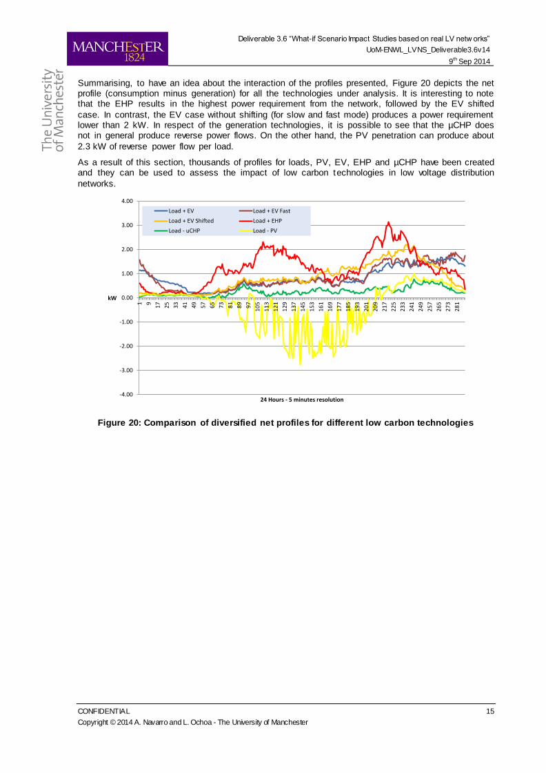
Summarising, to have an idea about the interaction of the profiles presented, Figure 20 depicts the net profile (consumption minus generation) for all the technologies under analysis. It is interesting to note that the EHP results in the highest power requirement from the network, followed by the EV shifted
case. In contrast, the EV case without shifting (for slow and fast mode) produces a power requirement lower than 2 kW. In respect of the generation technologies, it is possible to see that the µCHP does not in general produce reverse power flows. On the other hand, the PV penetration can produce about
2.3 kW of reverse power flow per load.
As a result of this section, thousands of profiles for loads, PV, EV, EHP and µCHP have been created and they can be used to assess the impact of low carbon technologies in low voltage distribution
networks.
Figure 20: Comparison of diversified net profiles for different low carbon technologies
-4.00
-3.00
-2.00
-1.00
0.00
1.00
2.00
3.00
4.00
1 9
17
25
33
41
49
57
65
73
81
89
97
10
5
11
3
12
1
12
9
13
7
14
5
15
3
16
1
16
9
17
7
18
5
19
3
20
1
20
9
21
7
22
5
23
3
24
1
24
9
25
7
26
5
27
3
28
1
kW
24 Hours - 5 minutes resolution
Load + EV Load + EV Fast
Load + EV Shifted Load + EHP
Load - uCHP Load - PV
Deliverable 3.6 “What-if Scenario Impact Studies based on real LV netw orks”
UoM-ENWL_LVNS_Deliverable3.6v14
9th Sep 2014
CONFIDENTIAL 16
Copyright © 2014 A. Navarro and L. Ochoa - The University of Manchester
3 LV Networks After the creation of the profiles of household loads and low carbon technologies, it is crucial to have realistic low voltage feeders to analyse the corresponding impacts. The information to create such networks was facilitated by ENWL through GIS files containing the network topology and the cable
characteristics (type of cable, phase connection, etc.). The main stages of this modelling process are the topology reconnection and the OpenDSS representation. Both of them are fully explained in Deliverable 1.2: “Tool for Translating Network Data from ENWL to OpenDSS” [13].
3.1 Modelling Summary
The first stage is needed because the ENWL GIS database presents many connections that seem
connected but in reality they are separated by very small distanced (from mm. to a couple of cm.). This does not allow power flow simulations given that all segments must be connected. To make the reconnection, the basic idea was to determine all the connected components (by using the Breath
First Search Algorithm) and then implementing the reconnection according to the distance among them. In this way, it is possible to have fully connected networks.
The power flow studies were carried out using OpenDSS, an open source software package to solve
power flows, harmonics analysis and fault current calculation in electrical distribution systems. One of the main characteristics of OpenDSS is the ability to represent the time dimension (daily and yearly simulations with different time step) in networks with distributed generation. This is very important to
measure the real impacts of intermittent sources (PV, micro-CHP, micron-wind turbines, etc.) and loads (EV, EHP etc.) on distribution networks. The second stage of the modelling process required all GIS files (fully connected) to be translated into OpenDSS format.
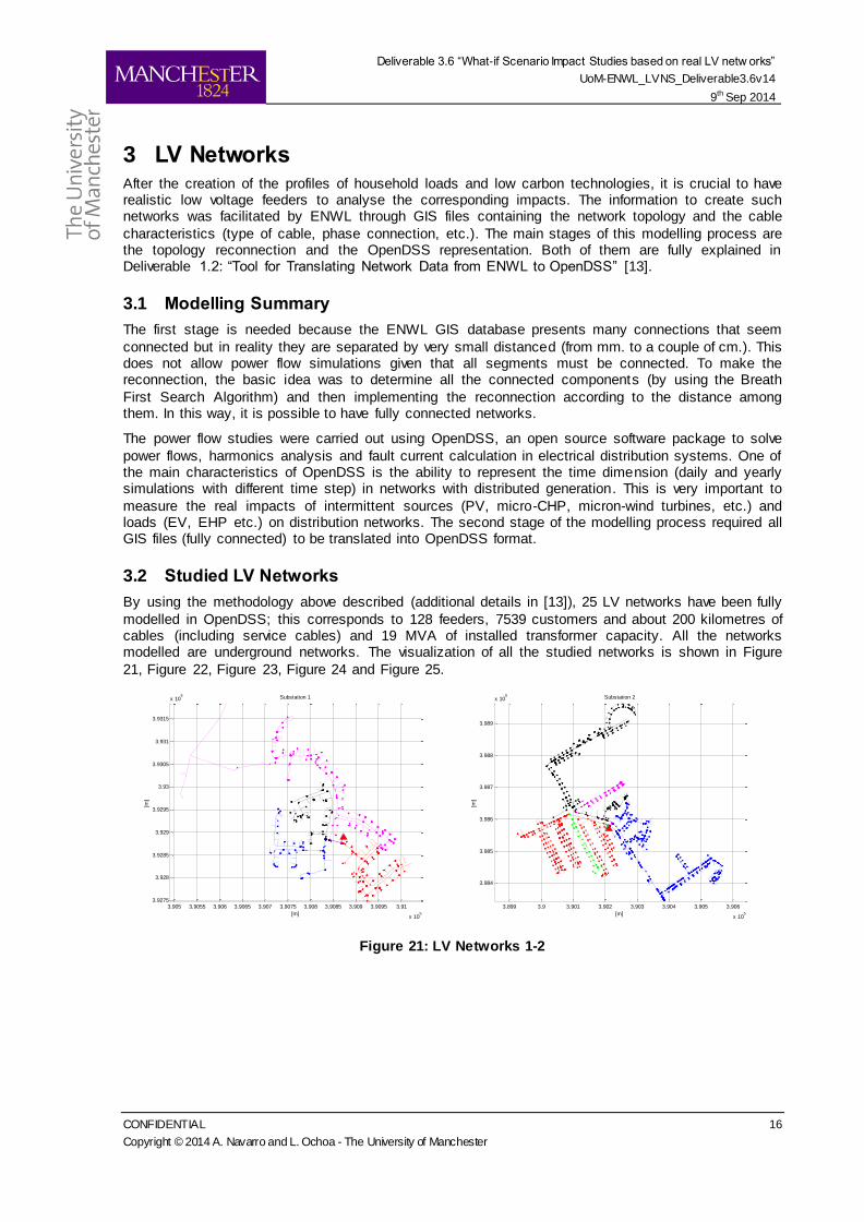
3.2 Studied LV Networks
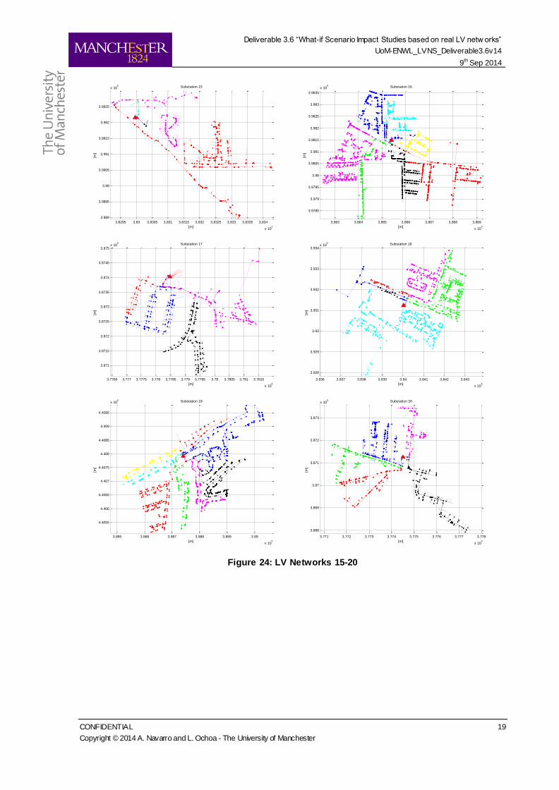
By using the methodology above described (additional details in [13]), 25 LV networks have been fully
modelled in OpenDSS; this corresponds to 128 feeders, 7539 customers and about 200 kilometres of cables (including service cables) and 19 MVA of installed transformer capacity. All the networks modelled are underground networks. The visualization of all the studied networks is shown in Figure
21, Figure 22, Figure 23, Figure 24 and Figure 25.
Figure 21: LV Networks 1-2
3.905 3.9055 3.906 3.9065 3.907 3.9075 3.908 3.9085 3.909 3.9095 3.91
x 105
3.9275
3.928
3.9285
3.929
3.9295
3.93
3.9305
3.931
3.9315
x 105
[m]
[m]
Substation 1
3.899 3.9 3.901 3.902 3.903 3.904 3.905 3.906
x 105
3.984
3.985
3.986
3.987
3.988
3.989
x 105
[m]
[m]
Substation 2
Deliverable 3.6 “What-if Scenario Impact Studies based on real LV netw orks”
UoM-ENWL_LVNS_Deliverable3.6v14
9th Sep 2014
CONFIDENTIAL 17
Copyright © 2014 A. Navarro and L. Ochoa - The University of Manchester
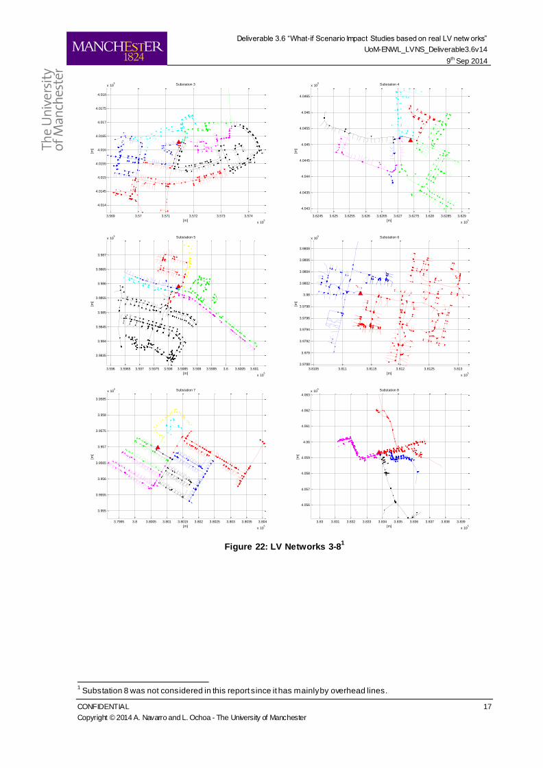
Figure 22: LV Networks 3-81
1 Substation 8 was not considered in this report since it has mainly by overhead lines.
3.569 3.57 3.571 3.572 3.573 3.574
x 105
4.014
4.0145
4.015
4.0155
4.016
4.0165
4.017
4.0175
4.018
x 105
[m]
[m]
Substation 3
3.6245 3.625 3.6255 3.626 3.6265 3.627 3.6275 3.628 3.6285 3.629
x 105
4.043
4.0435
4.044
4.0445
4.045
4.0455
4.046
4.0465
x 105
[m]
[m]
Substation 4
3.596 3.5965 3.597 3.5975 3.598 3.5985 3.599 3.5995 3.6 3.6005 3.601
x 105
3.9835
3.984
3.9845
3.985
3.9855
3.986
3.9865
3.987
x 105
[m]
[m]
Substation 5
3.8105 3.811 3.8115 3.812 3.8125 3.813
x 105
3.9788
3.979
3.9792
3.9794
3.9796
3.9798
3.98
3.9802
3.9804
3.9806
3.9808
x 105
[m]
[m]
Substation 6
3.7995 3.8 3.8005 3.801 3.8015 3.802 3.8025 3.803 3.8035 3.804
x 105
3.955
3.9555
3.956
3.9565
3.957
3.9575
3.958
3.9585
x 105
[m]
[m]
Substation 7
3.83 3.831 3.832 3.833 3.834 3.835 3.836 3.837 3.838 3.839
x 105
4.056
4.057
4.058
4.059
4.06
4.061
4.062
4.063x 10
5
[m]
[m]
Substation 8
Deliverable 3.6 “What-if Scenario Impact Studies based on real LV netw orks”
UoM-ENWL_LVNS_Deliverable3.6v14
9th Sep 2014
CONFIDENTIAL 18
Copyright © 2014 A. Navarro and L. Ochoa - The University of Manchester
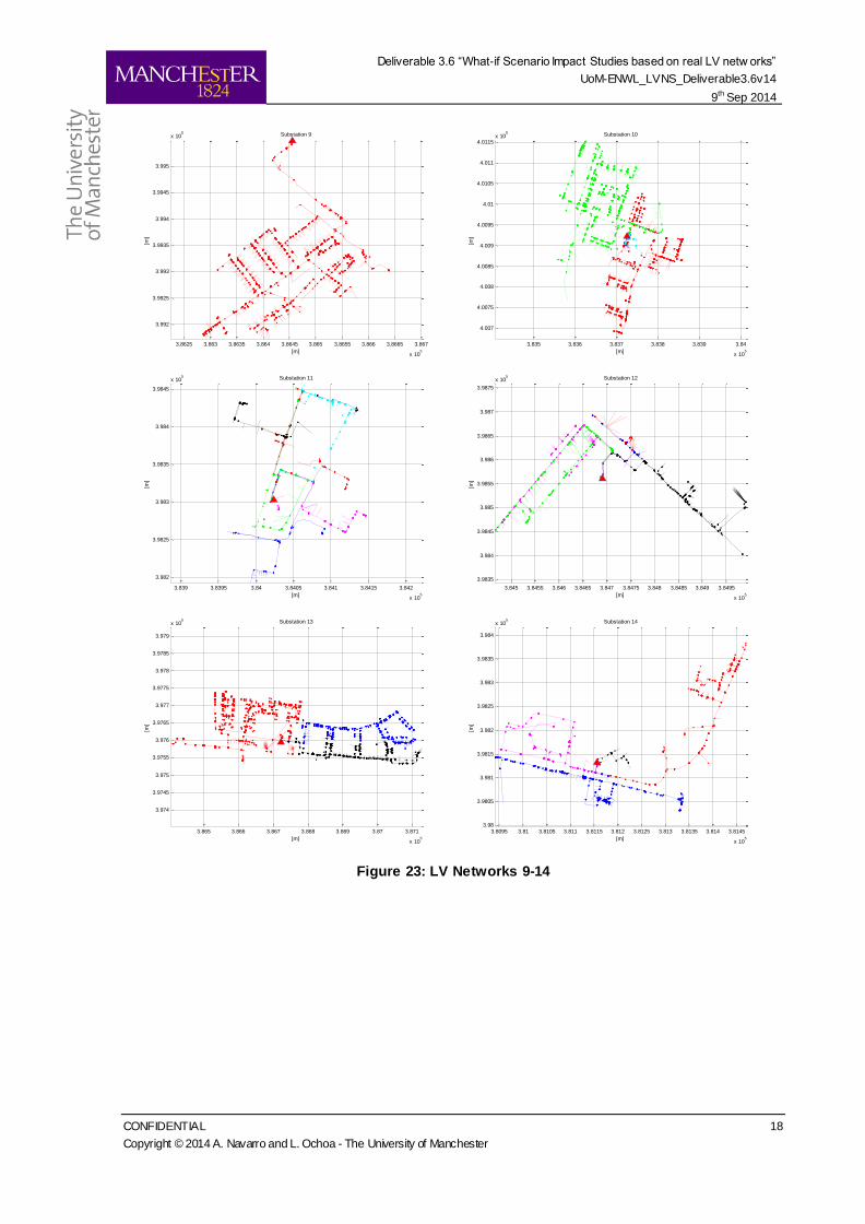
Figure 23: LV Networks 9-14
3.8625 3.863 3.8635 3.864 3.8645 3.865 3.8655 3.866 3.8665 3.867
x 105
3.992
3.9925
3.993
3.9935
3.994
3.9945
3.995
x 105
[m]
[m]
Substation 9
3.835 3.836 3.837 3.838 3.839 3.84
x 105
4.007
4.0075
4.008
4.0085
4.009
4.0095
4.01
4.0105
4.011
4.0115x 10
5
[m]
[m]
Substation 10
3.839 3.8395 3.84 3.8405 3.841 3.8415 3.842
x 105
3.982
3.9825
3.983
3.9835
3.984
3.9845
x 105
[m]
[m]
Substation 11
3.845 3.8455 3.846 3.8465 3.847 3.8475 3.848 3.8485 3.849 3.8495
x 105
3.9835
3.984
3.9845
3.985
3.9855
3.986
3.9865
3.987
3.9875
x 105
[m]
[m]
Substation 12
3.865 3.866 3.867 3.868 3.869 3.87 3.871
x 105
3.974
3.9745
3.975
3.9755
3.976
3.9765
3.977
3.9775
3.978
3.9785
3.979
x 105
[m]
[m]
Substation 13
3.8095 3.81 3.8105 3.811 3.8115 3.812 3.8125 3.813 3.8135 3.814 3.8145
x 105
3.98
3.9805
3.981
3.9815
3.982
3.9825
3.983
3.9835
3.984
x 105
[m]
[m]
Substation 14
Deliverable 3.6 “What-if Scenario Impact Studies based on real LV netw orks”
UoM-ENWL_LVNS_Deliverable3.6v14
9th Sep 2014
CONFIDENTIAL 19
Copyright © 2014 A. Navarro and L. Ochoa - The University of Manchester
Figure 24: LV Networks 15-20
3.8295 3.83 3.8305 3.831 3.8315 3.832 3.8325 3.833 3.8335 3.834
x 105
3.989
3.9895
3.99
3.9905
3.991
3.9915
3.992
3.9925
x 105
[m]
[m]
Substation 15
3.863 3.864 3.865 3.866 3.867 3.868 3.869
x 105
3.9785
3.979
3.9795
3.98
3.9805
3.981
3.9815
3.982
3.9825
3.983
3.9835
x 105
[m]
[m]
Substation 16
3.7765 3.777 3.7775 3.778 3.7785 3.779 3.7795 3.78 3.7805 3.781 3.7815
x 105
3.871
3.8715
3.872
3.8725
3.873
3.8735
3.874
3.8745
3.875x 10
5
[m]
[m]
Substation 17
3.836 3.837 3.838 3.839 3.84 3.841 3.842 3.843
x 105
3.928
3.929
3.93
3.931
3.932
3.933
3.934x 10
5
[m]
[m]
Substation 18
3.885 3.886 3.887 3.888 3.889 3.89
x 105
4.4055
4.406
4.4065
4.407
4.4075
4.408
4.4085
4.409
4.4095
x 105
[m]
[m]
Substation 19
3.771 3.772 3.773 3.774 3.775 3.776 3.777 3.778
x 105
3.868
3.869
3.87
3.871
3.872
3.873
x 105
[m]
[m]
Substation 20
Deliverable 3.6 “What-if Scenario Impact Studies based on real LV netw orks”
UoM-ENWL_LVNS_Deliverable3.6v14
9th Sep 2014
CONFIDENTIAL 20
Copyright © 2014 A. Navarro and L. Ochoa - The University of Manchester
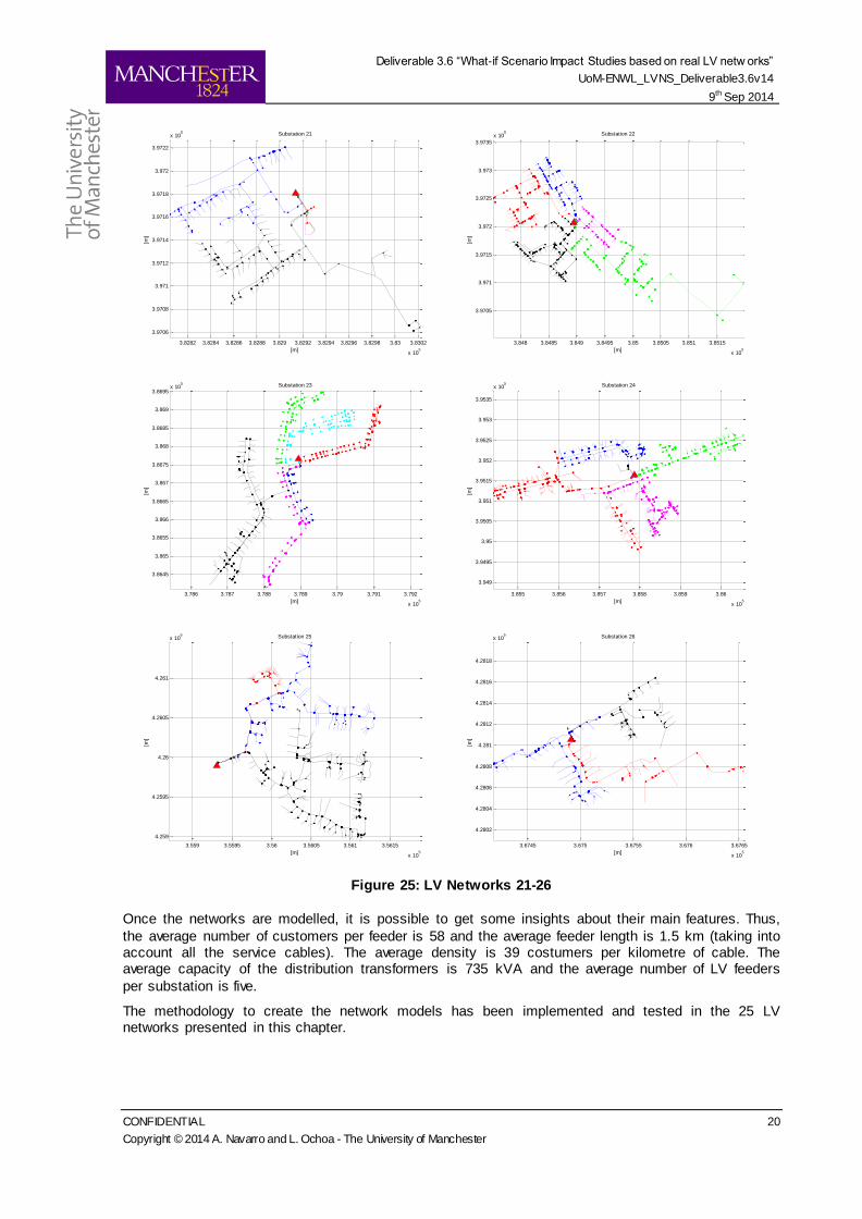
Figure 25: LV Networks 21-26
Once the networks are modelled, it is possible to get some insights about their main features. Thus,
the average number of customers per feeder is 58 and the average feeder length is 1.5 km (taking into account all the service cables). The average density is 39 costumers per kilometre of cable. The average capacity of the distribution transformers is 735 kVA and the average number of LV feeders
per substation is five.
The methodology to create the network models has been implemented and tested in the 25 LV networks presented in this chapter.
3.8282 3.8284 3.8286 3.8288 3.829 3.8292 3.8294 3.8296 3.8298 3.83 3.8302
x 105
3.9706
3.9708
3.971
3.9712
3.9714
3.9716
3.9718
3.972
3.9722
x 105
[m]
[m]
Substation 21
3.848 3.8485 3.849 3.8495 3.85 3.8505 3.851 3.8515
x 105
3.9705
3.971
3.9715
3.972
3.9725
3.973
3.9735
x 105
[m]
[m]
Substation 22
3.786 3.787 3.788 3.789 3.79 3.791 3.792
x 105
3.8645
3.865
3.8655
3.866
3.8665
3.867
3.8675
3.868
3.8685
3.869
3.8695x 10
5
[m]
[m]
Substation 23
3.855 3.856 3.857 3.858 3.859 3.86
x 105
3.949
3.9495
3.95
3.9505
3.951
3.9515
3.952
3.9525
3.953
3.9535
x 105
[m]
[m]
Substation 24
3.559 3.5595 3.56 3.5605 3.561 3.5615
x 105
4.259
4.2595
4.26
4.2605
4.261
x 105
[m]
[m]
Substation 25
3.6745 3.675 3.6755 3.676 3.6765
x 105
4.2802
4.2804
4.2806
4.2808
4.281
4.2812
4.2814
4.2816
4.2818
x 105
[m]
[m]
Substation 26
Deliverable 3.6 “What-if Scenario Impact Studies based on real LV netw orks”
UoM-ENWL_LVNS_Deliverable3.6v14
9th Sep 2014
CONFIDENTIAL 21
Copyright © 2014 A. Navarro and L. Ochoa - The University of Manchester
4 Probabilistic Impact Assessment Methodology The objective of the methodology presented in this section is to assess the expected impacts on low voltage distribution networks due to the penetration of low carbon technologies under different scenarios. The profiles and feeders used in this chapter correspond to the ones presented in chapters
2 and 3, respectively.
4.1 Literature Review
Several papers have focus on different aspects related to the penetration of DG in distribution systems. Most of them by using simplified networks or American real-life networks (much smaller LV networks than the European case). In [14], the maximum amount of DG that an LV feeder can host
without exhibiting under and/or over voltage problems is determined. The network implemented is a meshed USA distribution network (13.8kV/120 and 138kV/208V) with 311 loads. The study is, however, limited to maximum generation and minimum load (no time-series analysis) but adopts a
Monte Carlo approach for the DG location and size. The simulations are executed in a three-phase power flow engine. The utilization of energy storage systems to avoid the peak generation from the PV panels is proposed in [15]. This is particularly done to tackle the unbalance problems related with the
uneven distribution of PV connections (and injections). However, a simplified network is used and only a couple of scenarios with different generation and demand are simulated.
A proper alternative to cope with typical uncertainty of the low carbon technologies (location of DG,
size of the DG, load behaviour, etc.) is presented in [16]. Here, a Monte Carlo process is implemented to model the location and size of a single CHP (combined heat and power) plant in the network under study. Unfortunately, this work only uses a fictitious network (LV feeder supplying a circular area) and
the power flow model is a single-phase representation (balanced case). A more simplified study is presented in [17], where a basic framework regarding PV penetration limits in radial distribution systems, focusing on voltage rises and cable ratings is presented. However, the analysis is based on
a two-bus network with balanced loads. In contrast, the work presented in [18] implements a real Canadian residential suburban feeder (running a three-phase unbalanced case), providing an assessment on voltage profiles in residential neighbourhoods in the presence of PV. The analysis is
carried out only for certain scenarios (no time-series analysis). Furthermore, several real networks are implemented in [19]. The 16 LV feeders analysed correspond to U.S radial feeders simulated with a three-phase unbalanced power flow. They are studied by using a time-series simulation framework but
only with hourly resolution.
4.2 Methodology
From the studies described above, there are several analysis about DG impacts with different characteristics (time series, peak demand, balanced power flow, unbalance power flow, Monte Carlo Analysis, deterministic scenarios, etc.). Nonetheless, at the moment there are no analyses combining
the following features at the same time: Monte Carlo analysis, time-series simulation, unbalance power flows, and real-life networks (European style). The impact assessment methodology presented in this section considers all of these characteristics [20], [21]. The main steps are described below and
also summarised in Figure 26.
1. Firstly, different load profiles are allocated to each load in the feeder. These load profiles are randomly selected from the pool created in section 2.1 in order to represent properly the
diversity among the residential customers.
2. Secondly, for a given penetration level (from 0 to 100% in steps of 10%), the houses to have the analysed low carbon technology (LCT) are randomly selected. In this work, the penetration
level is defined as the percentage of houses with the LCT under analysis. Thus, if the penetration level is 20%, then 20% of the houses are selected to install a given technology. For example, the size of each PV panel is randomly selected according to the distribution of
residential PV panels in the UK (as presented in section 2.2). It is important to remark that the sun profile used for all the houses in the feeder is the same (assumption: there are not big changes in a small geographical region). Specifically, for the simulations presented in this
report, only the sunniest days are considered. In fact, the random sun profile is chosen among
Deliverable 3.6 “What-if Scenario Impact Studies based on real LV netw orks”
UoM-ENWL_LVNS_Deliverable3.6v14
9th Sep 2014
CONFIDENTIAL 22
Copyright © 2014 A. Navarro and L. Ochoa - The University of Manchester
the thirty sunniest days of the year. The idea behind this assumption is to assess the worst case scenario, avoiding the analysis of very cloudy days. This random selection is also applied for EV, EHP and µCHP. This probabilistic process is carried out to cater for the
uncertainties related to the location, size and behaviour of these technologies.
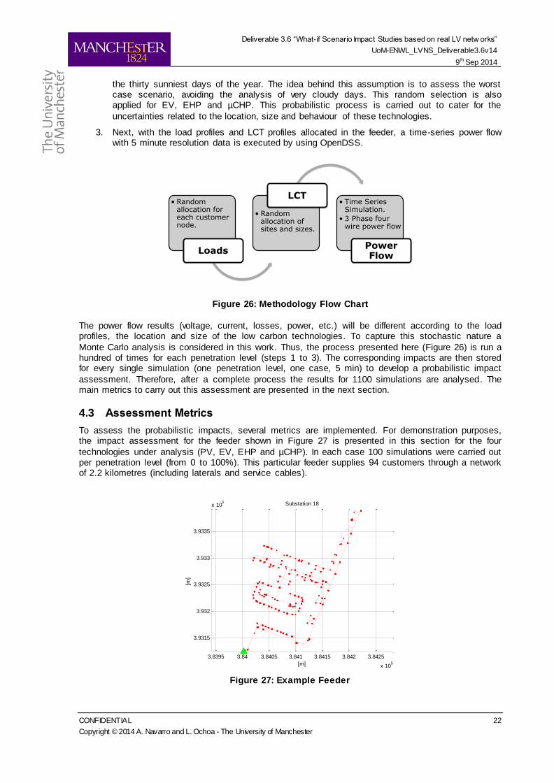
3. Next, with the load profiles and LCT profiles allocated in the feeder, a time-series power flow with 5 minute resolution data is executed by using OpenDSS.
Figure 26: Methodology Flow Chart
The power flow results (voltage, current, losses, power, etc.) will be different according to the load profiles, the location and size of the low carbon technologies. To capture this stochastic nature a
Monte Carlo analysis is considered in this work. Thus, the process presented here (Figure 26) is run a hundred of times for each penetration level (steps 1 to 3). The corresponding impacts are then stored for every single simulation (one penetration level, one case, 5 min) to develop a probabilistic impact
assessment. Therefore, after a complete process the results for 1100 simulations are analysed. The main metrics to carry out this assessment are presented in the next section.
4.3 Assessment Metrics
To assess the probabilistic impacts, several metrics are implemented. For demonstration purposes, the impact assessment for the feeder shown in Figure 27 is presented in this section for the four
technologies under analysis (PV, EV, EHP and µCHP). In each case 100 simulations were carried out per penetration level (from 0 to 100%). This particular feeder supplies 94 customers through a network of 2.2 kilometres (including laterals and service cables).
Figure 27: Example Feeder
• Random allocation for each customer node.
Loads
• Random allocation of sites and sizes.
LCT• Time Series
Simulation.
• 3 Phase four wire power flow
Power Flow
3.8395 3.84 3.8405 3.841 3.8415 3.842 3.8425
x 105
3.9315
3.932
3.9325
3.933
3.9335
x 105
[m]
[m]
Substation 18
Deliverable 3.6 “What-if Scenario Impact Studies based on real LV netw orks”
UoM-ENWL_LVNS_Deliverable3.6v14
9th Sep 2014
CONFIDENTIAL 23
Copyright © 2014 A. Navarro and L. Ochoa - The University of Manchester
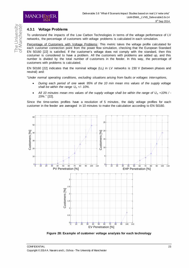
4.3.1 Voltage Problems
To understand the impacts of the Low Carbon Technologies in terms of the voltage performance of LV
networks, the percentage of customers with voltage problems is calculated in each simulation.
Percentage of Customers with Voltage Problems: This metric takes the voltage profile calculated for each customer connection point from the power flow simulation, checking that the European Standard
EN 50160 [22] is satisfied. If the customer’s voltage does not comply with the standard, then this costumer is considered to have a problem. All the customers with problems are added up, and this number is divided by the total number of customers in the feeder. In this way, the percentage of
customers with problems is calculated.
EN 50160 [22] indicates that the nominal voltage (Un) in LV networks is 230 V (between phases and neutral) and:
“Under normal operating conditions, excluding situations arising from faults or voltages interruptions,
During each period of one week 95% of the 10 min mean rms values of the supply voltage shall be within the range Un +/- 10%.
All 10 minutes mean rms values of the supply voltage shall be within the range of Un +10% / -15%.” [22].
Since the time-series profiles have a resolution of 5 minutes, the daily voltage profiles for each
customer in the feeder are averaged in 10 minutes to make the calculation according to EN 50160.
Figure 28: Example of customer voltage analysis for each technology
0 10 20 30 40 50 60 70 80 90 100 1100
10
20
30
40
50
60
PV Penetration [%]
Cu
sto
me
rs [
%]
0 10 20 30 40 50 60 70 80 90 100 1100
5
10
15
20
25
EHP Penetration [%]
Cu
sto
me
rs [
%]
0 10 20 30 40 50 60 70 80 90 100 1100
0.5
1
1.5
2
2.5
3
EV Penetration [%]
Cu
sto
me
rs [
%]
Deliverable 3.6 “What-if Scenario Impact Studies based on real LV netw orks”
UoM-ENWL_LVNS_Deliverable3.6v14
9th Sep 2014
CONFIDENTIAL 24
Copyright © 2014 A. Navarro and L. Ochoa - The University of Manchester
Once, the percentage of customers with voltage problems is calculated for each simulation, the average and standard deviation is determined for each penetration level. These results are presented in Figure 28 for the four technologies, adopting the average value +/- one standard deviation. For
example, for the PV case, the problems, although limited to ~2% of the customers, start at 40% of penetration level (40% of the houses with a PV panel). At 60% of penetration, however, 10% of the customers (in average) is not within the statutory limits.
On the other hand, the EHP produces voltage problems at 60% of penetration level and the magnitude of the problems are lower than in the PV case. In fact, the same average 10% of customers with voltage problems is reached after the 80% of penetration level in the EHP case. It is important to
remark, that in order to avoid outliers (low probability events), these figures only plot the cases when at least in average 1% of the customers have a problem. Under this criterion, the EV does not present any voltage problems (it never has in average 1% of the customers with voltage problems). For
comparison purposes, Figure 28 presents for the EV case all the problems (including those below 1%), showing that just at 100% of penetration level occurs the first problems and in average these problems affect in average only to 0.7% of the customers. Figure 28 does not show the µCHP case
because no voltage problems are observed with the penetration of this technology.
To summarise, in this particular feeder, in terms of voltage problems, the adoption of PV produces higher and earlier impacts.
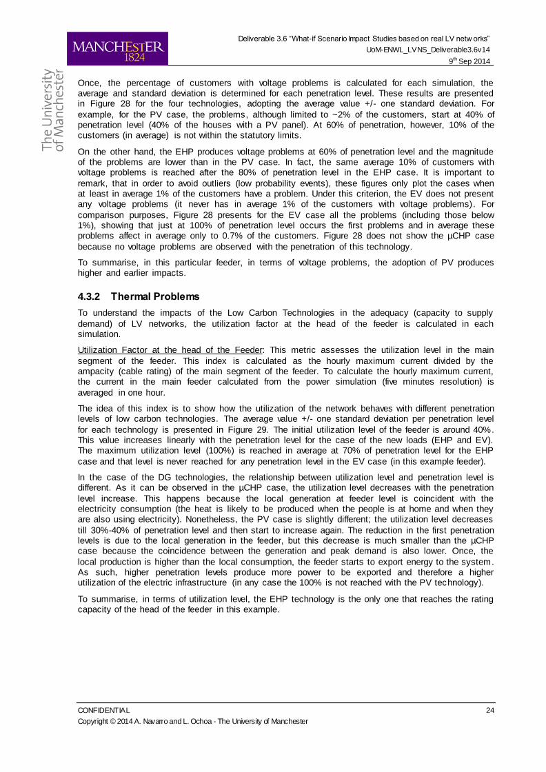
4.3.2 Thermal Problems
To understand the impacts of the Low Carbon Technologies in the adequacy (capacity to supply
demand) of LV networks, the utilization factor at the head of the feeder is calculated in each simulation.
Utilization Factor at the head of the Feeder: This metric assesses the utilization level in the main
segment of the feeder. This index is calculated as the hourly maximum current divided by the ampacity (cable rating) of the main segment of the feeder. To calculate the hourly maximum current, the current in the main feeder calculated from the power simulation (five minutes resolution) is
averaged in one hour.
The idea of this index is to show how the utilization of the network behaves with different penetration levels of low carbon technologies. The average value +/- one standard deviation per penetration level
for each technology is presented in Figure 29. The initial utilization level of the feeder is around 40%. This value increases linearly with the penetration level for the case of the new loads (EHP and EV). The maximum utilization level (100%) is reached in average at 70% of penetration level for the EHP
case and that level is never reached for any penetration level in the EV case (in this example feeder).
In the case of the DG technologies, the relationship between utilization level and penetration level is different. As it can be observed in the µCHP case, the utilization level decreases with the penetration
level increase. This happens because the local generation at feeder level is coincident with the electricity consumption (the heat is likely to be produced when the people is at home and when they are also using electricity). Nonetheless, the PV case is slightly different; the utilization level decreases
till 30%-40% of penetration level and then start to increase again. The reduction in the first penetration levels is due to the local generation in the feeder, but this decrease is much smaller than the µCHP case because the coincidence between the generation and peak demand is also lower. Once, the
local production is higher than the local consumption, the feeder starts to export energy to the system. As such, higher penetration levels produce more power to be exported and therefore a higher utilization of the electric infrastructure (in any case the 100% is not reached with the PV technology).
To summarise, in terms of utilization level, the EHP technology is the only one that reaches the rating capacity of the head of the feeder in this example.
Deliverable 3.6 “What-if Scenario Impact Studies based on real LV netw orks”
UoM-ENWL_LVNS_Deliverable3.6v14
9th Sep 2014
CONFIDENTIAL 25
Copyright © 2014 A. Navarro and L. Ochoa - The University of Manchester
Figure 29: Example of feeder utilization for each technology
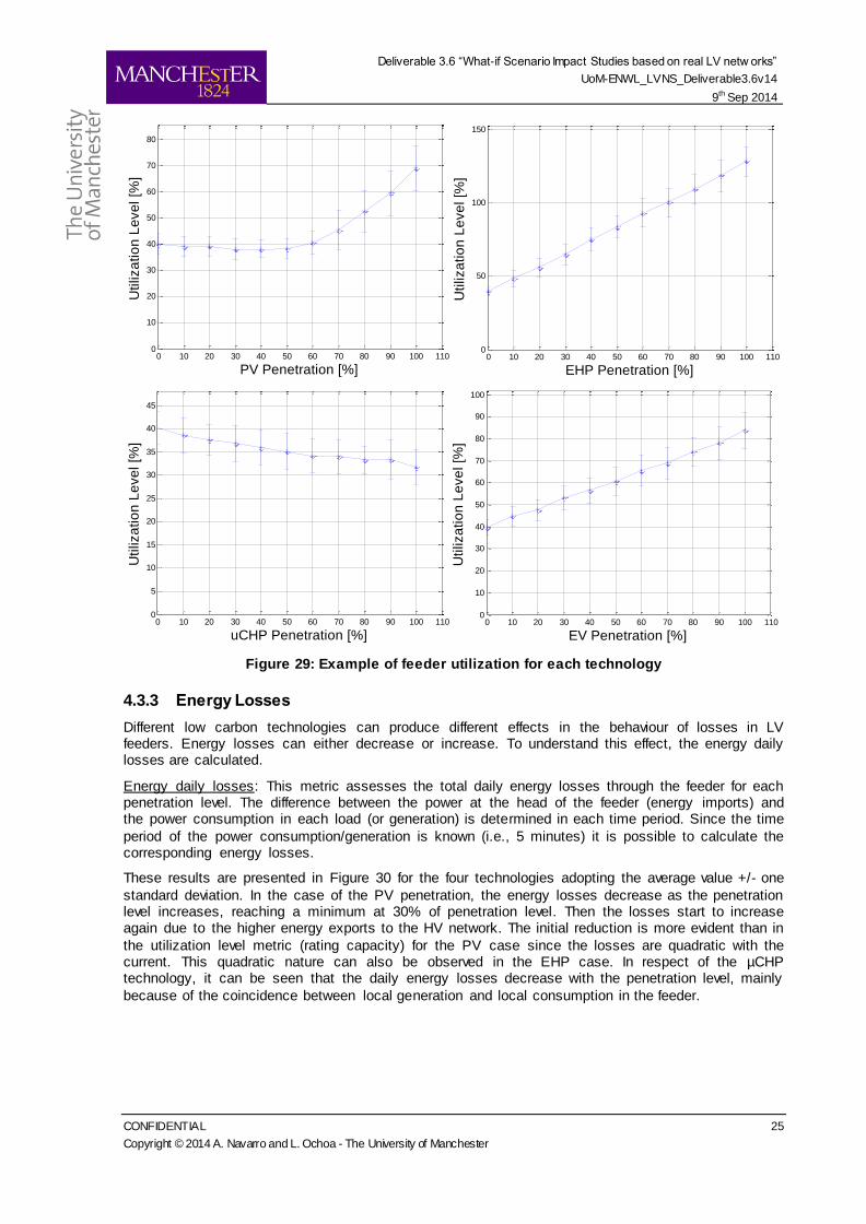
4.3.3 Energy Losses
Different low carbon technologies can produce different effects in the behaviour of losses in LV feeders. Energy losses can either decrease or increase. To understand this effect, the energy daily losses are calculated.
Energy daily losses: This metric assesses the total daily energy losses through the feeder for each penetration level. The difference between the power at the head of the feeder (energy imports) and the power consumption in each load (or generation) is determined in each time period. Since the time
period of the power consumption/generation is known (i.e., 5 minutes) it is possible to calculate the corresponding energy losses.
These results are presented in Figure 30 for the four technologies adopting the average value +/- one
standard deviation. In the case of the PV penetration, the energy losses decrease as the penetration level increases, reaching a minimum at 30% of penetration level. Then the losses start to increase again due to the higher energy exports to the HV network. The initial reduction is more evident than in
the utilization level metric (rating capacity) for the PV case since the losses are quadratic with the current. This quadratic nature can also be observed in the EHP case. In respect of the µCHP technology, it can be seen that the daily energy losses decrease with the penetration level, mainly
because of the coincidence between local generation and local consumption in the feeder.
0 10 20 30 40 50 60 70 80 90 100 1100
10
20
30
40
50
60
70
80
PV Penetration [%]
Utiliza
tio
n L
eve
l [%
]
0 10 20 30 40 50 60 70 80 90 100 1100
50
100
150
EHP Penetration [%]
Utiliza
tio
n L
eve
l [%
]
0 10 20 30 40 50 60 70 80 90 100 1100
5
10
15
20
25
30
35
40
45
uCHP Penetration [%]
Utiliza
tio
n L
eve
l [%
]
0 10 20 30 40 50 60 70 80 90 100 1100
10
20
30
40
50
60
70
80
90
100
EV Penetration [%]
Utiliza
tio
n L
eve
l [%
]
Deliverable 3.6 “What-if Scenario Impact Studies based on real LV netw orks”
UoM-ENWL_LVNS_Deliverable3.6v14
9th Sep 2014
CONFIDENTIAL 26
Copyright © 2014 A. Navarro and L. Ochoa - The University of Manchester
Figure 30: Example of daily energy losses for each technology
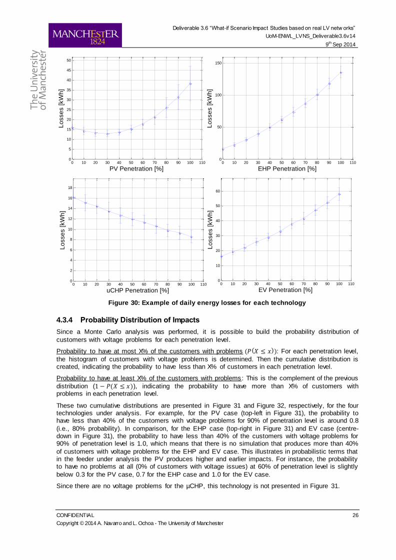
4.3.4 Probability Distribution of Impacts
Since a Monte Carlo analysis was performed, it is possible to build the probability distribution of
customers with voltage problems for each penetration level.
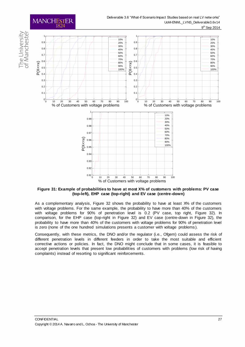
Probability to have at most X% of the customers with problems )): For each penetration level,
the histogram of customers with voltage problems is determined. Then the cumulative distribution is created, indicating the probability to have less than X% of customers in each penetration level.
Probability to have at least X% of the customers with problems: This is the complement of the previous
distribution ( )), indicating the probability to have more than X% of customers with problems in each penetration level.
These two cumulative distributions are presented in Figure 31 and Figure 32, respectively, for the four technologies under analysis. For example, for the PV case (top-left in Figure 31), the probability to have less than 40% of the customers with voltage problems for 90% of penetration level is around 0.8
(i.e., 80% probability). In comparison, for the EHP case (top-right in Figure 31) and EV case (centre-down in Figure 31), the probability to have less than 40% of the customers with voltage problems for 90% of penetration level is 1.0, which means that there is no simulation that produces more than 40%
of customers with voltage problems for the EHP and EV case. This illustrates in probabilistic terms that in the feeder under analysis the PV produces higher and earlier impacts. For instance, the probability to have no problems at all (0% of customers with voltage issues) at 60% of penetration level is slightly
below 0.3 for the PV case, 0.7 for the EHP case and 1.0 for the EV case.
Since there are no voltage problems for the µCHP, this technology is not presented in Figure 31.
0 10 20 30 40 50 60 70 80 90 100 1100
5
10
15
20
25
30
35
40
45
50
PV Penetration [%]
Lo
sse
s [
kW
h]
0 10 20 30 40 50 60 70 80 90 100 1100
50
100
150
EHP Penetration [%]
Lo
sse
s [
kW
h]
0 10 20 30 40 50 60 70 80 90 100 1100
2
4
6
8
10
12
14
16
18
uCHP Penetration [%]
Lo
sse
s [
kW
h]
0 10 20 30 40 50 60 70 80 90 100 1100
10
20
30
40
50
60
EV Penetration [%]
Lo
sse
s [
kW
h]
Deliverable 3.6 “What-if Scenario Impact Studies based on real LV netw orks”
UoM-ENWL_LVNS_Deliverable3.6v14
9th Sep 2014
CONFIDENTIAL 27
Copyright © 2014 A. Navarro and L. Ochoa - The University of Manchester
Figure 31: Example of probabilities to have at most X% of customers with problems: PV case (top-left), EHP case (top-right) and EV case (centre-down)
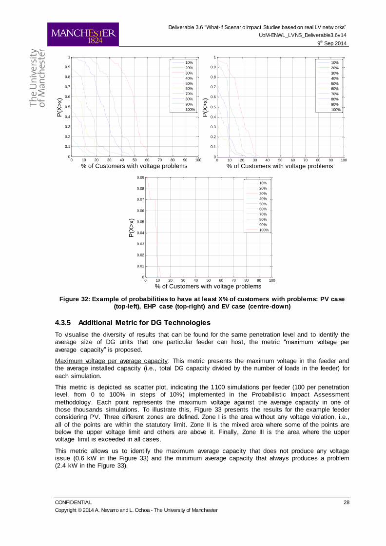
As a complementary analysis, Figure 32 shows the probability to have at least X% of the customers
with voltage problems. For the same example, the probability to have more than 40% of the customers with voltage problems for 90% of penetration level is 0.2 (PV case, top right, Figure 32). In comparison, for the EHP case (top-right in Figure 32) and EV case (centre-down in Figure 32), the
probability to have more than 40% of the customers with voltage problems for 90% of penetration level is zero (none of the one hundred simulations presents a customer with voltage problems).
Consequently, with these metrics, the DNO and/or the regulator (i.e., Ofgem) could assess the risk of
different penetration levels in different feeders in order to take the most suitable and efficient corrective actions or policies. In fact, the DNO might conclude that in some cases, it is feasible to accept penetration levels that present low probabilit ies of customers with problems (low risk of having
complaints) instead of resorting to significant reinforcements.
0 10 20 30 40 50 60 70 80 90 1000
0.1
0.2
0.3
0.4
0.5
0.6
0.7
0.8
0.9
1
% of Customers with voltage problems
P(X
<=
x)
10%
20%
30%
40%
50%
60%
70%
80%
90%
100%
0 10 20 30 40 50 60 70 80 90 1000
0.1
0.2
0.3
0.4
0.5
0.6
0.7
0.8
0.9
1
% of Customers with voltage problems
P(X
<=
x)
10%
20%
30%
40%
50%
60%
70%
80%
90%
100%
0 10 20 30 40 50 60 70 80 90 1000.91
0.92
0.93
0.94
0.95
0.96
0.97
0.98
0.99
1
% of Customers with voltage problems
P(X
<=
x)
10%
20%
30%
40%
50%
60%
70%
80%
90%
100%
Deliverable 3.6 “What-if Scenario Impact Studies based on real LV netw orks”
UoM-ENWL_LVNS_Deliverable3.6v14
9th Sep 2014
CONFIDENTIAL 28
Copyright © 2014 A. Navarro and L. Ochoa - The University of Manchester
Figure 32: Example of probabilities to have at least X% of customers with problems: PV case (top-left), EHP case (top-right) and EV case (centre-down)
4.3.5 Additional Metric for DG Technologies
To visualise the diversity of results that can be found for the same penetration level and to identify the average size of DG units that one particular feeder can host, the metric “maximum voltage per
average capacity” is proposed.
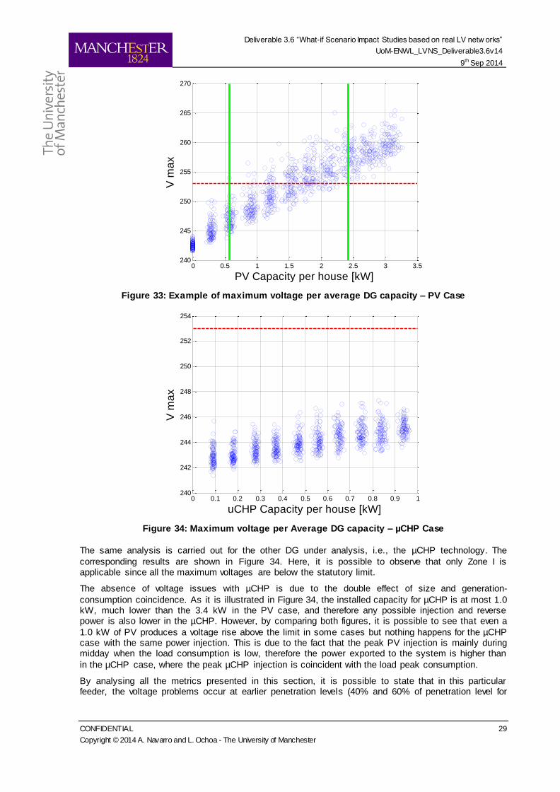
Maximum voltage per average capacity: This metric presents the maximum voltage in the feeder and the average installed capacity (i.e., total DG capacity divided by the number of loads in the feeder) for
each simulation.
This metric is depicted as scatter plot, indicating the 1100 simulations per feeder (100 per penetration level, from 0 to 100% in steps of 10%) implemented in the Probabilistic Impact Assessment
methodology. Each point represents the maximum voltage against the average capacity in one of those thousands simulations. To illustrate this, Figure 33 presents the results for the example feeder considering PV. Three different zones are defined. Zone I is the area without any voltage violation, i.e.,
all of the points are within the statutory limit. Zone II is the mixed area where some of the points are below the upper voltage limit and others are above it. Finally, Zone III is the area where the upper voltage limit is exceeded in all cases.
This metric allows us to identify the maximum average capacity that does not produce any voltage issue (0.6 kW in the Figure 33) and the minimum average capacity that always produces a problem (2.4 kW in the Figure 33).
0 10 20 30 40 50 60 70 80 90 1000
0.1
0.2
0.3
0.4
0.5
0.6
0.7
0.8
0.9
1
% of Customers with voltage problems
P(X
>x)
10%
20%
30%
40%
50%
60%
70%
80%
90%
100%
0 10 20 30 40 50 60 70 80 90 1000
0.1
0.2
0.3
0.4
0.5
0.6
0.7
0.8
0.9
1
% of Customers with voltage problems
P(X
>x)
10%
20%
30%
40%
50%
60%
70%
80%
90%
100%
0 10 20 30 40 50 60 70 80 90 1000
0.01
0.02
0.03
0.04
0.05
0.06
0.07
0.08
0.09
% of Customers with voltage problems
P(X
>x)
10%
20%
30%
40%
50%
60%
70%
80%
90%
100%
Deliverable 3.6 “What-if Scenario Impact Studies based on real LV netw orks”
UoM-ENWL_LVNS_Deliverable3.6v14
9th Sep 2014
CONFIDENTIAL 29
Copyright © 2014 A. Navarro and L. Ochoa - The University of Manchester
Figure 33: Example of maximum voltage per average DG capacity – PV Case
Figure 34: Maximum voltage per Average DG capacity – µCHP Case
The same analysis is carried out for the other DG under analysis, i.e., the µCHP technology. The
corresponding results are shown in Figure 34. Here, it is possible to observe that only Zone I is applicable since all the maximum voltages are below the statutory limit.
The absence of voltage issues with µCHP is due to the double effect of size and generation-
consumption coincidence. As it is illustrated in Figure 34, the installed capacity for µCHP is at most 1.0 kW, much lower than the 3.4 kW in the PV case, and therefore any possible injection and reverse power is also lower in the µCHP. However, by comparing both figures, it is possible to see that even a
1.0 kW of PV produces a voltage rise above the limit in some cases but nothing happens for the µCHP case with the same power injection. This is due to the fact that the peak PV injection is mainly during midday when the load consumption is low, therefore the power exported to the system is higher than
in the µCHP case, where the peak µCHP injection is coincident with the load peak consumption.
By analysing all the metrics presented in this section, it is possible to state that in this particular feeder, the voltage problems occur at earlier penetration levels (40% and 60% of penetration level for
0 0.5 1 1.5 2 2.5 3 3.5240
245
250
255
260
265
270
PV Capacity per house [kW]
V m
ax
0 0.1 0.2 0.3 0.4 0.5 0.6 0.7 0.8 0.9 1240
242
244
246
248
250
252
254
uCHP Capacity per house [kW]
V m
ax
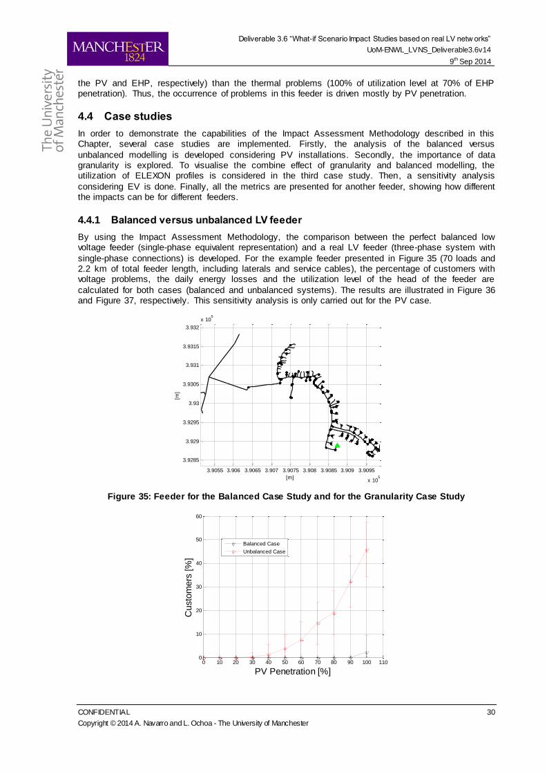
Deliverable 3.6 “What-if Scenario Impact Studies based on real LV netw orks”
UoM-ENWL_LVNS_Deliverable3.6v14
9th Sep 2014
CONFIDENTIAL 30
Copyright © 2014 A. Navarro and L. Ochoa - The University of Manchester
the PV and EHP, respectively) than the thermal problems (100% of utilization level at 70% of EHP penetration). Thus, the occurrence of problems in this feeder is driven mostly by PV penetration.
4.4 Case studies
In order to demonstrate the capabilities of the Impact Assessment Methodology described in this Chapter, several case studies are implemented. Firstly, the analysis of the balanced versus
unbalanced modelling is developed considering PV installations. Secondly, the importance of data granularity is explored. To visualise the combine effect of granularity and balanced modelling, the utilization of ELEXON profiles is considered in the third case study. Then, a sensitivity analysis
considering EV is done. Finally, all the metrics are presented for another feeder, showing how different the impacts can be for different feeders.
4.4.1 Balanced versus unbalanced LV feeder
By using the Impact Assessment Methodology, the comparison between the perfect balanced low voltage feeder (single-phase equivalent representation) and a real LV feeder (three-phase system with
single-phase connections) is developed. For the example feeder presented in Figure 35 (70 loads and 2.2 km of total feeder length, including laterals and service cables), the percentage of customers with voltage problems, the daily energy losses and the utilization level of the head of the feeder are
calculated for both cases (balanced and unbalanced systems). The results are illustrated in Figure 36 and Figure 37, respectively. This sensitivity analysis is only carried out for the PV case.
Figure 35: Feeder for the Balanced Case Study and for the Granularity Case Study
3.9055 3.906 3.9065 3.907 3.9075 3.908 3.9085 3.909 3.9095
x 105
3.9285
3.929
3.9295
3.93
3.9305
3.931
3.9315
3.932
x 105
[m]
[m]
0 10 20 30 40 50 60 70 80 90 100 1100
10
20
30
40
50
60
PV Penetration [%]
Custo
mers
[%
]
Balanced Case
Unbalanced Case
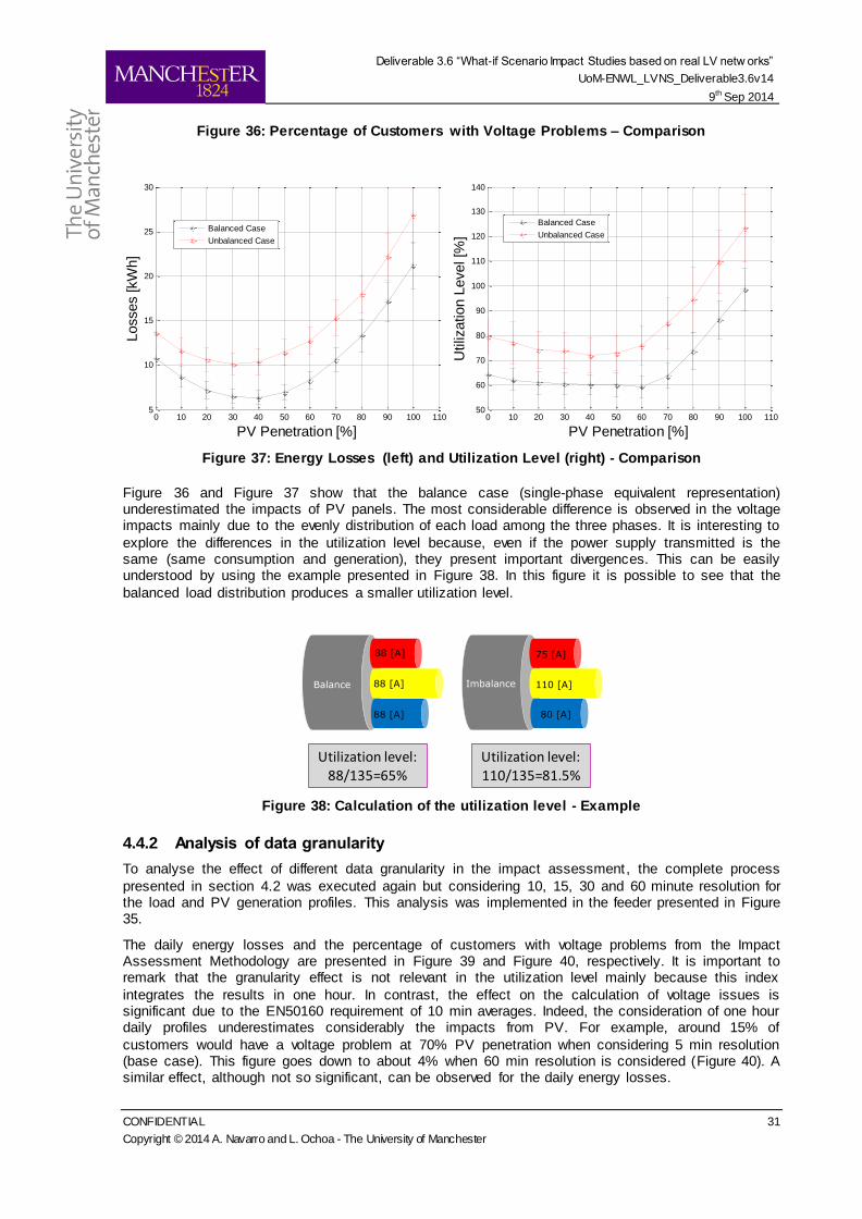
Deliverable 3.6 “What-if Scenario Impact Studies based on real LV netw orks”
UoM-ENWL_LVNS_Deliverable3.6v14
9th Sep 2014
CONFIDENTIAL 31
Copyright © 2014 A. Navarro and L. Ochoa - The University of Manchester
Figure 36: Percentage of Customers with Voltage Problems – Comparison
Figure 37: Energy Losses (left) and Utilization Level (right) - Comparison
Figure 36 and Figure 37 show that the balance case (single-phase equivalent representation) underestimated the impacts of PV panels. The most considerable difference is observed in the voltage impacts mainly due to the evenly distribution of each load among the three phases. It is interesting to
explore the differences in the utilization level because, even if the power supply transmitted is the same (same consumption and generation), they present important divergences. This can be easily understood by using the example presented in Figure 38. In this figure it is possible to see that the
balanced load distribution produces a smaller utilization level.
Figure 38: Calculation of the utilization level - Example
4.4.2 Analysis of data granularity
To analyse the effect of different data granularity in the impact assessment, the complete process
presented in section 4.2 was executed again but considering 10, 15, 30 and 60 minute resolution for the load and PV generation profiles. This analysis was implemented in the feeder presented in Figure 35.
The daily energy losses and the percentage of customers with voltage problems from the Impact Assessment Methodology are presented in Figure 39 and Figure 40, respectively. It is important to remark that the granularity effect is not relevant in the utilization level mainly because this index
integrates the results in one hour. In contrast, the effect on the calculation of voltage issues is significant due to the EN50160 requirement of 10 min averages. Indeed, the consideration of one hour daily profiles underestimates considerably the impacts from PV. For example, around 15% of
customers would have a voltage problem at 70% PV penetration when considering 5 min resolution (base case). This figure goes down to about 4% when 60 min resolution is considered (Figure 40). A similar effect, although not so significant, can be observed for the daily energy losses.
0 10 20 30 40 50 60 70 80 90 100 1105
10
15
20
25
30
PV Penetration [%]
Losses [kW
h]
Balanced Case
Unbalanced Case
0 10 20 30 40 50 60 70 80 90 100 11050
60
70
80
90
100
110
120
130
140
PV Penetration [%]
Utiliz
ation L
evel [%
]
Balanced Case
Unbalanced Case
110 [A]
80 [A]
75 [A]
Imbalance
88 [A]
88 [A]
88 [A]
Balance
Utilization level:110/135=81.5%
Utilization level:88/135=65%
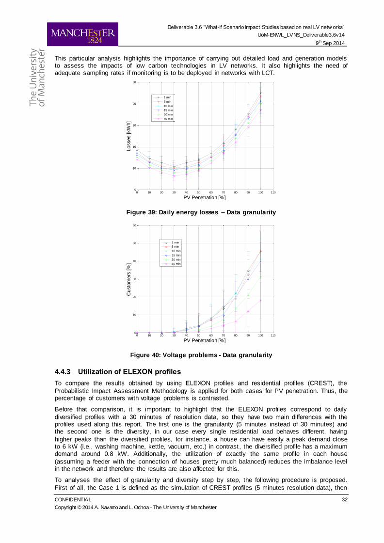
Deliverable 3.6 “What-if Scenario Impact Studies based on real LV netw orks”
UoM-ENWL_LVNS_Deliverable3.6v14
9th Sep 2014
CONFIDENTIAL 32
Copyright © 2014 A. Navarro and L. Ochoa - The University of Manchester
This particular analysis highlights the importance of carrying out detailed load and generation models to assess the impacts of low carbon technologies in LV networks. It also highlights the need of adequate sampling rates if monitoring is to be deployed in networks with LCT.
Figure 39: Daily energy losses – Data granularity
Figure 40: Voltage problems - Data granularity
4.4.3 Utilization of ELEXON profiles
To compare the results obtained by using ELEXON profiles and residential profiles (CREST), the
Probabilistic Impact Assessment Methodology is applied for both cases for PV penetration. Thus, the percentage of customers with voltage problems is contrasted.
Before that comparison, it is important to highlight that the ELEXON profiles correspond to daily
diversified profiles with a 30 minutes of resolution data, so they have two main differences with the profiles used along this report. The first one is the granularity (5 minutes instead of 30 minutes) and the second one is the diversity, in our case every single residential load behaves different, having
higher peaks than the diversified profiles, for instance, a house can have easily a peak demand close to 6 kW (i.e., washing machine, kettle, vacuum, etc.) in contrast , the diversified profile has a maximum demand around 0.8 kW. Additionally, the utilization of exactly the same profile in each house
(assuming a feeder with the connection of houses pretty much balanced) reduces the imbalance level in the network and therefore the results are also affected for this.
To analyses the effect of granularity and diversity step by step, the following procedure is proposed.
First of all, the Case 1 is defined as the simulation of CREST profiles (5 minutes resolution data), then
0 10 20 30 40 50 60 70 80 90 100 1105
10
15
20
25
30
PV Penetration [%]
Losses [kW
h]
1 min
5 min
10 min
15 min
30 min
60 min
0 10 20 30 40 50 60 70 80 90 100 1100
10
20
30
40
50
60
PV Penetration [%]
Custo
mers
[%
]
1 min
5 min
10 min
15 min
30 min
60 min
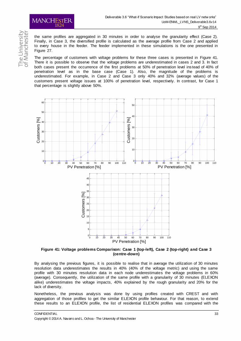
Deliverable 3.6 “What-if Scenario Impact Studies based on real LV netw orks”
UoM-ENWL_LVNS_Deliverable3.6v14
9th Sep 2014
CONFIDENTIAL 33
Copyright © 2014 A. Navarro and L. Ochoa - The University of Manchester
the same profiles are aggregated in 30 minutes in order to analyse the granularity effect (Case 2). Finally, in Case 3, the diversified profile is calculated as the average profile from Case 2 and applied to every house in the feeder. The feeder implemented in these simulations is the one presented in
Figure 27.
The percentage of customers with voltage problems for these three cases is presented in Figure 41. There it is possible to observe that the voltage problems are underestimated in cases 2 and 3. In fact
both cases present the occurrence of the first problems at 50% of penetration level ins tead of 40% of penetration level as in the base case (Case 1). Also, the magnitude of the problems is underestimated. For example, in Case 2 and Case 3 only 40% and 32% (average values) of the
customers present voltage issues at 100% of penetration level, respectively. In contrast, for Case 1 that percentage is slightly above 50%.
Figure 41: Voltage problems Comparison: Case 1 (top-left), Case 2 (top-right) and Case 3 (centre-down)
By analysing the previous figures, it is possible to realise that in average the utilization of 30 minutes
resolution data underestimates the results in 40% (40% of the voltage metric) and using the same profile with 30 minutes resolution data in each node underestimates the voltage problems in 60% (average). Consequently, the utilization of the same profile with a granularity of 30 minutes (ELEXON
alike) underestimates the voltage impacts, 40% explained by the rough granularity and 20% for the lack of diversity.
Nonetheless, the previous analysis was done by using profiles created with CREST and with
aggregation of those profiles to get the similar ELEXON profile behaviour. For that reason, to extend these results to an ELEXON profile, the list of residential ELEXON profiles was compared with the
0 10 20 30 40 50 60 70 80 90 100 1100
10
20
30
40
50
60
PV Penetration [%]
Custo
mers
[%
]
0 10 20 30 40 50 60 70 80 90 100 1100
10
20
30
40
50
PV Penetration [%]
Custo
mers
[%
]
0 10 20 30 40 50 60 70 80 90 100 1100
5
10
15
20
25
30
35
40
45
PV Penetration [%]
Custo
mers
[%
]
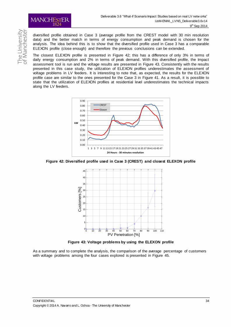
Deliverable 3.6 “What-if Scenario Impact Studies based on real LV netw orks”
UoM-ENWL_LVNS_Deliverable3.6v14
9th Sep 2014
CONFIDENTIAL 34
Copyright © 2014 A. Navarro and L. Ochoa - The University of Manchester
diversified profile obtained in Case 3 (average profile from the CREST model with 30 min resolution data) and the better match in terms of energy consumption and peak demand is chosen for the analysis. The idea behind this is to show that the diversified profile used in Case 3 has a comparable
ELEXON profile (close enough) and therefore the previous conclusions can be extended.
The closest ELEXON profile is presented in Figure 42; this has a difference of only 3% in terms of daily energy consumption and 2% in terms of peak demand. With this diversified profile, the Impact
assessment tool is run and the voltage results are presented in Figure 43. Consistently with the results presented in this case study, the utilization of ELEXON profiles underestimates the assessment of voltage problems in LV feeders. It is interesting to note that, as expected, the results for the ELEXON
profile case are similar to the ones presented for the Case 3 in Figure 41. As a result, it is possible to state that the utilization of ELEXON profiles at residential level underestimates the technical impacts along the LV feeders.
Figure 42: Diversified profile used in Case 3 (CREST) and closest ELEXON profile
Figure 43: Voltage problems by using the ELEXON profile
As a summary and to complete the analysis, the comparison of the average percentage of customers with voltage problems among the four cases explored is presented in Figure 45.
0.00
0.10
0.20
0.30
0.40
0.50
0.60
0.70
0.80
0.90
1 3 5 7 9 11 13 15 17 19 21 23 25 27 29 31 33 35 37 39 41 43 45 47
kW
24 Hours - 30 minutes resolution
CREST
Elexon
0 10 20 30 40 50 60 70 80 90 100 1100
5
10
15
20
25
30
35
40
45
PV Penetration [%]
Custo
mers
[%
]
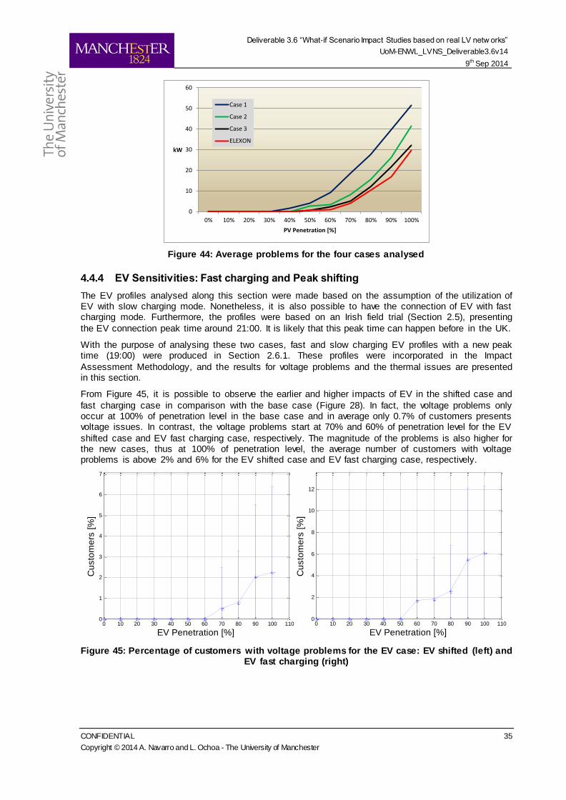
Deliverable 3.6 “What-if Scenario Impact Studies based on real LV netw orks”
UoM-ENWL_LVNS_Deliverable3.6v14
9th Sep 2014
CONFIDENTIAL 35
Copyright © 2014 A. Navarro and L. Ochoa - The University of Manchester
Figure 44: Average problems for the four cases analysed
4.4.4 EV Sensitivities: Fast charging and Peak shifting
The EV profiles analysed along this section were made based on the assumption of the utilization of EV with slow charging mode. Nonetheless, it is also possible to have the connection of EV with fast charging mode. Furthermore, the profiles were based on an Irish field trial (Section 2.5), presenting
the EV connection peak time around 21:00. It is likely that this peak time can happen before in the UK.
With the purpose of analysing these two cases, fast and slow charging EV profiles with a new peak time (19:00) were produced in Section 2.6.1. These profiles were incorporated in the Impact
Assessment Methodology, and the results for voltage problems and the thermal issues are presented in this section.
From Figure 45, it is possible to observe the earlier and higher impacts of EV in the shifted case and
fast charging case in comparison with the base case (Figure 28). In fact, the voltage problems only occur at 100% of penetration level in the base case and in average only 0.7% of customers presents voltage issues. In contrast, the voltage problems start at 70% and 60% of penetration level for the EV
shifted case and EV fast charging case, respectively. The magnitude of the problems is also higher for the new cases, thus at 100% of penetration level, the average number of customers with voltage problems is above 2% and 6% for the EV shifted case and EV fast charging case, respectively.
Figure 45: Percentage of customers with voltage problems for the EV case: EV shifted (left) and EV fast charging (right)
0
10
20
30
40
50
60
0% 10% 20% 30% 40% 50% 60% 70% 80% 90% 100%
kW
PV Penetration [%]
Case 1
Case 2
Case 3
ELEXON
0 10 20 30 40 50 60 70 80 90 100 1100
1
2
3
4
5
6
7
EV Penetration [%]
Cu
sto
me
rs [
%]
0 10 20 30 40 50 60 70 80 90 100 1100
2
4
6
8
10
12
EV Penetration [%]
Cu
sto
me
rs [
%]
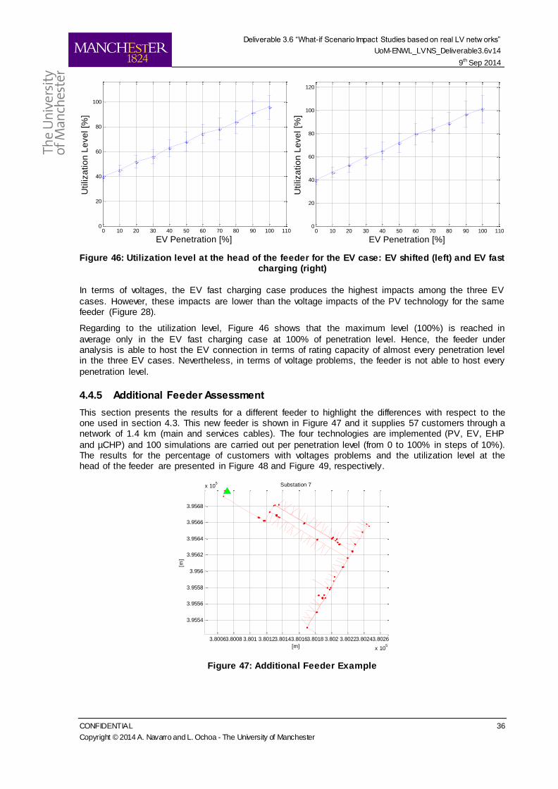
Deliverable 3.6 “What-if Scenario Impact Studies based on real LV netw orks”
UoM-ENWL_LVNS_Deliverable3.6v14
9th Sep 2014
CONFIDENTIAL 36
Copyright © 2014 A. Navarro and L. Ochoa - The University of Manchester
Figure 46: Utilization level at the head of the feeder for the EV case: EV shifted (left) and EV fast charging (right)
In terms of voltages, the EV fast charging case produces the highest impacts among the three EV
cases. However, these impacts are lower than the voltage impacts of the PV technology for the same feeder (Figure 28).
Regarding to the utilization level, Figure 46 shows that the maximum level (100%) is reached in
average only in the EV fast charging case at 100% of penetration level. Hence, the feeder under analysis is able to host the EV connection in terms of rating capacity of almost every penetration level in the three EV cases. Nevertheless, in terms of voltage problems, the feeder is not able to host every
penetration level.
4.4.5 Additional Feeder Assessment
This section presents the results for a different feeder to highlight the differences with respect to the one used in section 4.3. This new feeder is shown in Figure 47 and it supplies 57 customers through a network of 1.4 km (main and services cables). The four technologies are implemented (PV, EV, EHP
and µCHP) and 100 simulations are carried out per penetration level (from 0 to 100% in steps of 10%). The results for the percentage of customers with voltages problems and the utilization level at the head of the feeder are presented in Figure 48 and Figure 49, respectively.
Figure 47: Additional Feeder Example
0 10 20 30 40 50 60 70 80 90 100 1100
20
40
60
80
100
EV Penetration [%]
Utiliza
tio
n L
eve
l [%
]
0 10 20 30 40 50 60 70 80 90 100 1100
20
40
60
80
100
120
EV Penetration [%]
Utiliza
tio
n L
eve
l [%
]
3.80063.8008 3.801 3.80123.80143.80163.8018 3.802 3.80223.80243.8026
x 105
3.9554
3.9556
3.9558
3.956
3.9562
3.9564
3.9566
3.9568
x 105
[m]
[m]
Substation 7
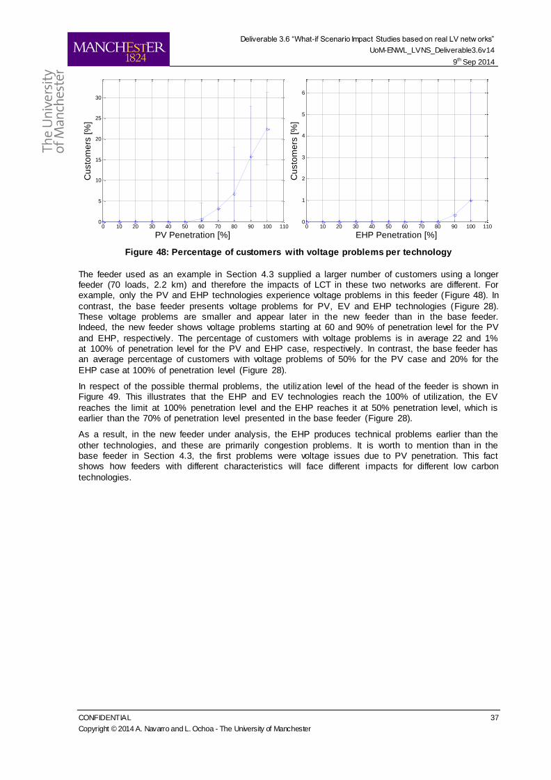
Deliverable 3.6 “What-if Scenario Impact Studies based on real LV netw orks”
UoM-ENWL_LVNS_Deliverable3.6v14
9th Sep 2014
CONFIDENTIAL 37
Copyright © 2014 A. Navarro and L. Ochoa - The University of Manchester
Figure 48: Percentage of customers with voltage problems per technology
The feeder used as an example in Section 4.3 supplied a larger number of customers using a longer feeder (70 loads, 2.2 km) and therefore the impacts of LCT in these two networks are different. For example, only the PV and EHP technologies experience voltage problems in this feeder (Figure 48). In
contrast, the base feeder presents voltage problems for PV, EV and EHP technologies (Figure 28). These voltage problems are smaller and appear later in the new feeder than in the base feeder. Indeed, the new feeder shows voltage problems starting at 60 and 90% of penetration level for the PV
and EHP, respectively. The percentage of customers with voltage problems is in average 22 and 1% at 100% of penetration level for the PV and EHP case, respectively. In contrast, the base feeder has an average percentage of customers with voltage problems of 50% for the PV case and 20% for the
EHP case at 100% of penetration level (Figure 28).
In respect of the possible thermal problems, the utilization level of the head of the feeder is shown in Figure 49. This illustrates that the EHP and EV technologies reach the 100% of utilization, the EV
reaches the limit at 100% penetration level and the EHP reaches it at 50% penetration level, which is earlier than the 70% of penetration level presented in the base feeder (Figure 28).
As a result, in the new feeder under analysis, the EHP produces technical problems earlier than the
other technologies, and these are primarily congestion problems. It is worth to mention than in the base feeder in Section 4.3, the first problems were voltage issues due to PV penetration. This fact shows how feeders with different characteristics will face different impacts for different low carbon
technologies.
0 10 20 30 40 50 60 70 80 90 100 1100
5
10
15
20
25
30
PV Penetration [%]
Cu
sto
me
rs [
%]
0 10 20 30 40 50 60 70 80 90 100 1100
1
2
3
4
5
6
EHP Penetration [%]
Cu
sto
me
rs [
%]
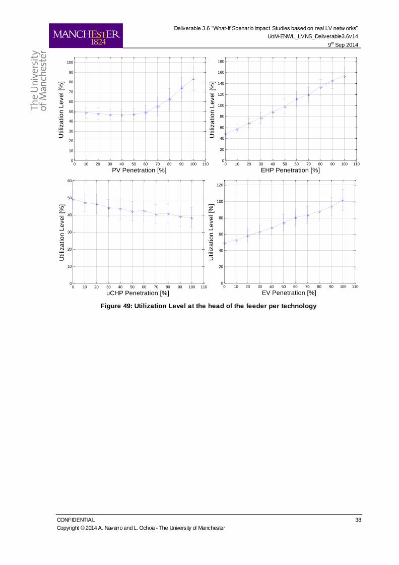
Deliverable 3.6 “What-if Scenario Impact Studies based on real LV netw orks”
UoM-ENWL_LVNS_Deliverable3.6v14
9th Sep 2014
CONFIDENTIAL 38
Copyright © 2014 A. Navarro and L. Ochoa - The University of Manchester
Figure 49: Utilization Level at the head of the feeder per technology
0 10 20 30 40 50 60 70 80 90 100 1100
10
20
30
40
50
60
70
80
90
100
PV Penetration [%]
Utiliza
tio
n L
eve
l [%
]
0 10 20 30 40 50 60 70 80 90 100 1100
20
40
60
80
100
120
140
160
180
EHP Penetration [%]
Utiliza
tio
n L
eve
l [%
]
0 10 20 30 40 50 60 70 80 90 100 1100
10
20
30
40
50
60
uCHP Penetration [%]
Utiliza
tio
n L
eve
l [%
]
0 10 20 30 40 50 60 70 80 90 100 1100
20
40
60
80
100
120
EV Penetration [%]
Utiliza
tio
n L
eve
l [%
]

Deliverable 3.6 “What-if Scenario Impact Studies based on real LV netw orks”
UoM-ENWL_LVNS_Deliverable3.6v14
9th Sep 2014
CONFIDENTIAL 39
Copyright © 2014 A. Navarro and L. Ochoa - The University of Manchester
5 Multi-Feeder Analysis The Impact Assessment Methodology implemented in Chapter 4 is useful for understanding the behaviour of one particular feeder under different penetration levels of low carbon technologies. Nonetheless, the lessons obtained from one feeder cannot be necessarily extrapolated to a different
one. In fact, the two feeders compared in section 4.4.5 face the occurrence of the first problems at different penetration levels. It is for that reason, that a larger number of feeders are analysed in this section.
The main idea is to apply the Probabilistic Impact Assessment Methodology over hundreds of feeders in order to get some general lessons about the impacts of low carbon technologies in LV networks. By analysing specific characteristics of LV networks (e.g., number of customers, feeder length, etc.) this
methodology can also be used to find the corresponding correlation with the potential impacts of LCT. Ultimately, this correlation can then be adopted by Distribution Network Operators to directly quantify those impacts without the need of further detailed network analyses.
The Probabilistic Impact Assessment Methodology is applied to 128 feeders. All the low carbon technologies (PV, EV, EHP and µCHP) are investigated considering daily profiles with 5 minutes resolution data and running 100 simulations for each penetration level for each feeder under analysis.
The voltage reference implemented at the secondary of the transformer is 241V phase to neutral (1.05 p.u.) in order to have the same headroom for voltage drops and voltage rises due to the penetration of DG and new loads, respectively. Nevertheless, there could be some very long feeders that might
present under voltage problems at 0% of penetration level (without any low carbon technology) with this reference voltage. To solve this problem, the reference voltage (secondary of the transformer) is increased gradually with the purpose of avoiding any under voltage issue. For this, an ADMD of 1.5
kW is first allocated to each load (according to ENWL’s planning criteria [23]) to then calculate the voltage for the last customer running a power flow. This voltage cannot be lower than 0.94 p.u. For example, if the feeder has an under voltage problem with 241V, then the voltage is increased by 1%.
This process is repeated till the problem is solved (no more than 255V are considered). Consequently, once the problem is solved, the Probabilistic Impact Assessment Methodology is executed.
5.1 Results Overview
5.1.1 General Analysis
After the application of the Probabilistic Impact Assessment Methodology in each of the 128 feeders under analysis for each of the technologies, it is possible to get a general overview about how problematic are the different technologies and what type of technical problem (voltage or thermal
issues) is more likely to occur.
The percentages of feeders that present voltage problems or thermal problems for at least one of the penetration levels are illustrated in Figure 50. For instance, 45% of the feeders experience voltage
problems and almost 10% of feeders reach the 100% of utilization level in the PV case. In contrast, in the EHP case, the percentage of feeders with voltage and thermal problems is 30% and 39%, respectively. It is worth mentioning that less than 4% of the feeders present problems in the µCHP
case, and these problems are only related with voltage rise.
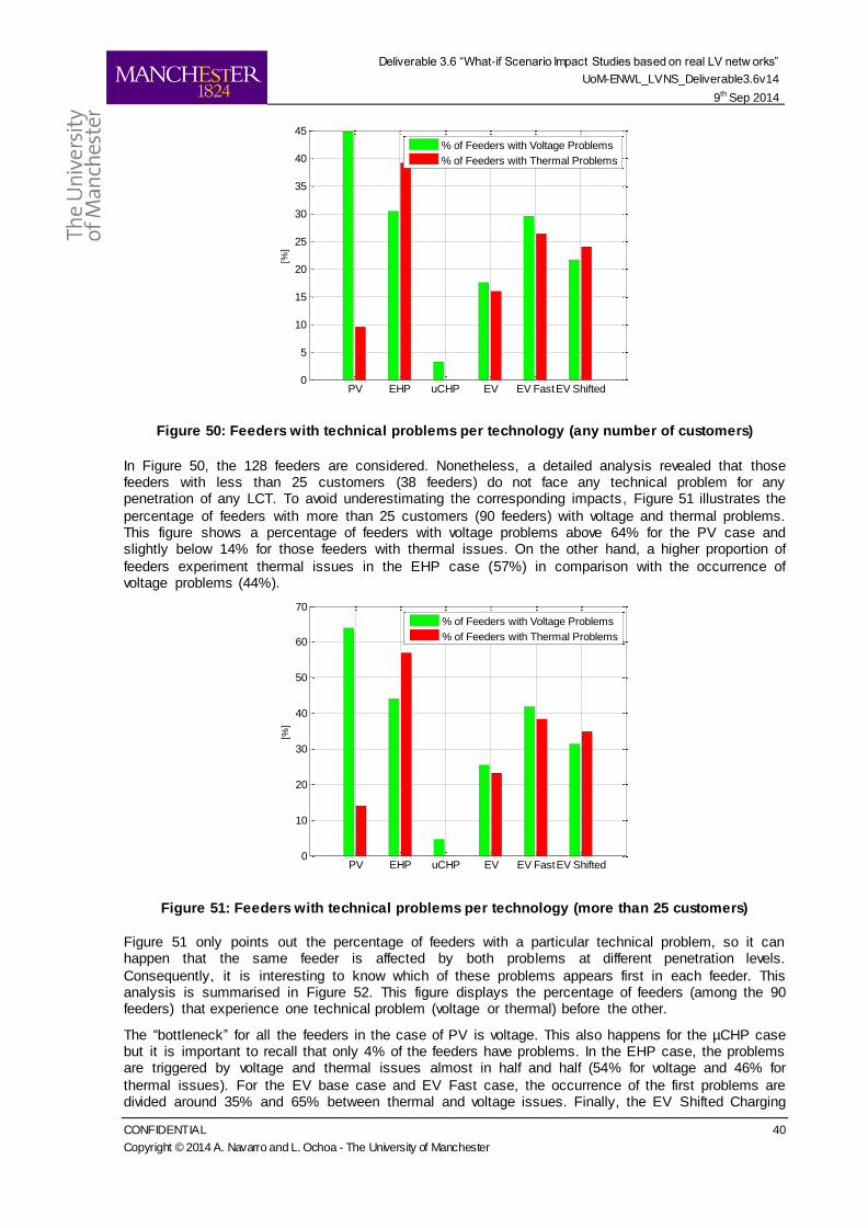
Deliverable 3.6 “What-if Scenario Impact Studies based on real LV netw orks”
UoM-ENWL_LVNS_Deliverable3.6v14
9th Sep 2014
CONFIDENTIAL 40
Copyright © 2014 A. Navarro and L. Ochoa - The University of Manchester
Figure 50: Feeders with technical problems per technology (any number of customers)
In Figure 50, the 128 feeders are considered. Nonetheless, a detailed analysis revealed that those feeders with less than 25 customers (38 feeders) do not face any technical problem for any penetration of any LCT. To avoid underestimating the corresponding impacts, Figure 51 illustrates the
percentage of feeders with more than 25 customers (90 feeders) with voltage and thermal problems. This figure shows a percentage of feeders with voltage problems above 64% for the PV case and slightly below 14% for those feeders with thermal issues. On the other hand, a higher proportion of
feeders experiment thermal issues in the EHP case (57%) in comparison with the occurrence of voltage problems (44%).
Figure 51: Feeders with technical problems per technology (more than 25 customers)
Figure 51 only points out the percentage of feeders with a particular technical problem, so it can happen that the same feeder is affected by both problems at different penetration levels.
Consequently, it is interesting to know which of these problems appears first in each feeder. This analysis is summarised in Figure 52. This figure displays the percentage of feeders (among the 90 feeders) that experience one technical problem (voltage or thermal) before the other.
The “bottleneck” for all the feeders in the case of PV is voltage. This also happens for the µCHP case but it is important to recall that only 4% of the feeders have problems. In the EHP case, the problems are triggered by voltage and thermal issues almost in half and half (54% for voltage and 46% for
thermal issues). For the EV base case and EV Fast case, the occurrence of the first problems are divided around 35% and 65% between thermal and voltage issues. Finally, the EV Shifted Charging
PV EHP uCHP EV EV FastEV Shifted0
5
10
15
20
25
30
35
40
45
[%]
% of Feeders with Voltage Problems
% of Feeders with Thermal Problems
PV EHP uCHP EV EV FastEV Shifted0
10
20
30
40
50
60
70
[%]
% of Feeders with Voltage Problems
% of Feeders with Thermal Problems
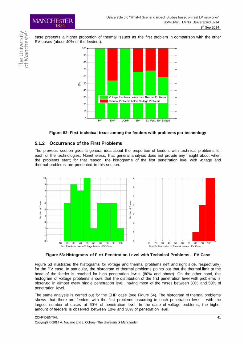
Deliverable 3.6 “What-if Scenario Impact Studies based on real LV netw orks”
UoM-ENWL_LVNS_Deliverable3.6v14
9th Sep 2014
CONFIDENTIAL 41
Copyright © 2014 A. Navarro and L. Ochoa - The University of Manchester
case presents a higher proportion of thermal issues as the first problem in comparison with the other EV cases (about 40% of the feeders).
Figure 52: First technical issue among the feeders with problems per technology
5.1.2 Occurrence of the First Problems
The previous section gives a general idea about the proportion of feeders with technical problems for
each of the technologies. Nonetheless, that general analysis does not provide any insight about when the problems start; for that reason, the histograms of the first penetration level with voltage and thermal problems are presented in this section.
Figure 53: Histograms of First Penetration Level with Technical Problems – PV Case
Figure 53 illustrates the histograms for voltage and thermal problems (left and right side, respectively) for the PV case. In particular, the histogram of thermal problems points out that the thermal limit at the
head of the feeder is reached for high penetration levels (80% and above). On the other hand, the histogram of voltage problems shows that the distribution of the first penetration level with problems is observed in almost every single penetration level, having most of the cases between 30% and 50% of
penetration level.
The same analysis is carried out for the EHP case (see Figure 54). The histogram of thermal problems shows that there are feeders with the first problems occurring in each penetration level – with the
largest number of cases at 60% of penetration level. In the case of voltage problems, the higher amount of feeders is observed between 10% and 30% of penetration level.
PV EHP uCHP EV EV Fast EV Shifted0
10
20
30
40
50
60
70
80
90
100
[%]
Voltage Problems before than Thermal Problems
Thermal Problems before Voltage Problems
10 20 30 40 50 60 70 80 90 1000
1
2
3
4
5
6
7
8
9
10
First Problems due to Voltage Issues - PV Case
Num
ber
of
Cases
10 20 30 40 50 60 70 80 90 1000
1
2
3
4
5
6
7
First Problems due to Thermal Issues - PV Case
Num
ber
of
Cases
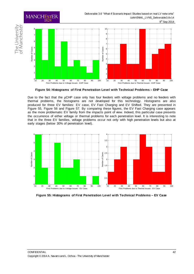
Deliverable 3.6 “What-if Scenario Impact Studies based on real LV netw orks”
UoM-ENWL_LVNS_Deliverable3.6v14
9th Sep 2014
CONFIDENTIAL 42
Copyright © 2014 A. Navarro and L. Ochoa - The University of Manchester
Figure 54: Histograms of First Penetration Level with Technical Problems – EHP Case
Due to the fact that the µCHP case only has four feeders with voltage problems and no feeders with thermal problems, the histograms are not developed for this technology. Histograms are also
produced for three EV families: EV case, EV Fast Charging and EV Shifted. They are presented in Figure 55, Figure 56 and Figure 57. By comparing these figures, the EV Fast Charging case appears as the more problematic EV family from the impacts point of view. Indeed, this particular case presents
the occurrence of either voltage or thermal problems for each penetration level. It is interesting to note that in the three EV families, voltage problems occur not only with high penetration levels but also at early stages (below 30% of penetration level).
Figure 55: Histograms of First Penetration Level with Technical Problems – EV Case
10 20 30 40 50 60 70 80 90 1000
1
2
3
4
5
6
7
8
First Problems due to Voltage Issues - EHP Case
Num
ber
of
Cases
10 20 30 40 50 60 70 80 90 1000
1
2
3
4
5
6
7
8
9
10
First Problems due to Thermal Issues - EHP Case
Num
ber
of
Cases
10 20 30 40 50 60 70 80 90 1000
1
2
3
4
5
6
First Problems due to Voltage Issues - EV Case
Num
ber
of
Cases
10 20 30 40 50 60 70 80 90 1000
0.5
1
1.5
2
2.5
3
3.5
4
First Problems due to Thermal Issues - EV Case
Num
ber
of
Cases
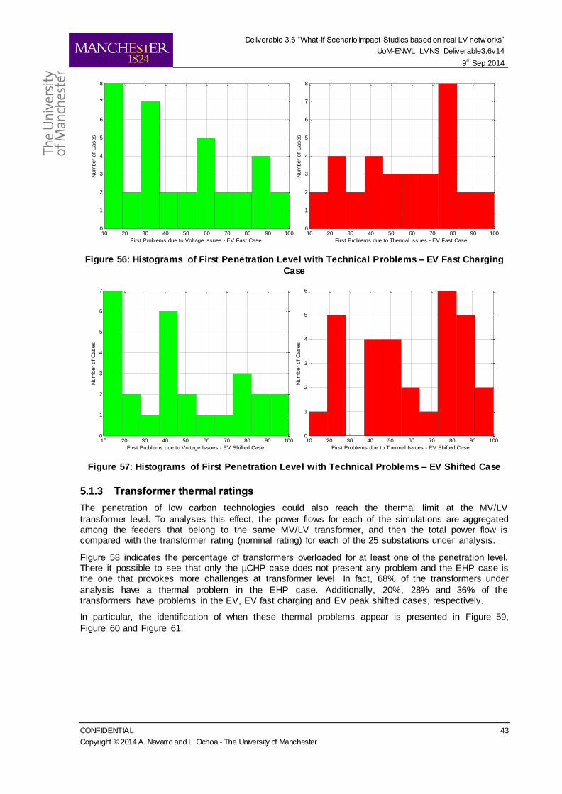
Deliverable 3.6 “What-if Scenario Impact Studies based on real LV netw orks”
UoM-ENWL_LVNS_Deliverable3.6v14
9th Sep 2014
CONFIDENTIAL 43
Copyright © 2014 A. Navarro and L. Ochoa - The University of Manchester
Figure 56: Histograms of First Penetration Level with Technical Problems – EV Fast Charging
Case
Figure 57: Histograms of First Penetration Level with Technical Problems – EV Shifted Case
5.1.3 Transformer thermal ratings
The penetration of low carbon technologies could also reach the thermal limit at the MV/LV
transformer level. To analyses this effect, the power flows for each of the simulations are aggregated among the feeders that belong to the same MV/LV transformer, and then the total power flow is compared with the transformer rating (nominal rating) for each of the 25 substations under analysis.
Figure 58 indicates the percentage of transformers overloaded for at least one of the penetration level. There it possible to see that only the µCHP case does not present any problem and the EHP case is the one that provokes more challenges at transformer level. In fact, 68% of the transformers under
analysis have a thermal problem in the EHP case. Additionally, 20%, 28% and 36% of the transformers have problems in the EV, EV fast charging and EV peak shifted cases, respectively.
In particular, the identification of when these thermal problems appear is presented in Figure 59,
Figure 60 and Figure 61.
10 20 30 40 50 60 70 80 90 1000
1
2
3
4
5
6
7
8
First Problems due to Voltage Issues - EV Fast Case
Num
ber
of
Cases
10 20 30 40 50 60 70 80 90 1000
1
2
3
4
5
6
7
8
First Problems due to Thermal Issues - EV Fast Case
Num
ber
of
Cases
10 20 30 40 50 60 70 80 90 1000
1
2
3
4
5
6
7
First Problems due to Voltage Issues - EV Shifted Case
Num
ber
of
Cases
10 20 30 40 50 60 70 80 90 1000
1
2
3
4
5
6
First Problems due to Thermal Issues - EV Shifted Case
Num
ber
of
Cases
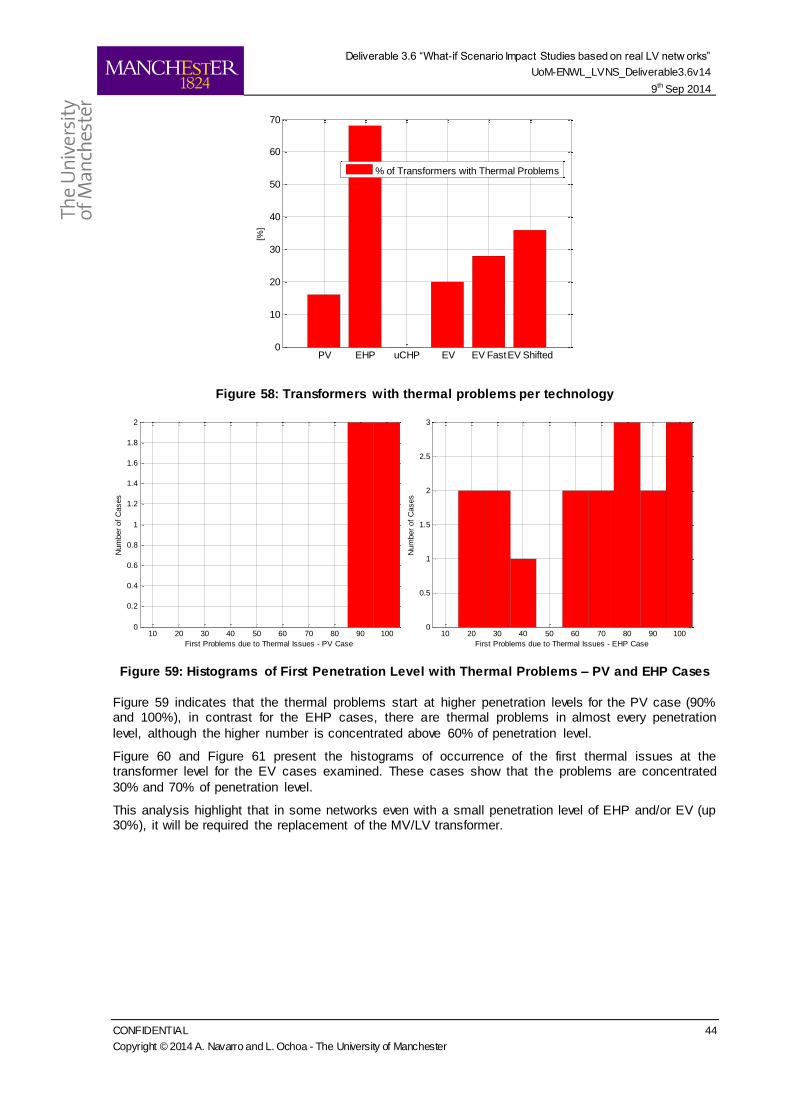
Deliverable 3.6 “What-if Scenario Impact Studies based on real LV netw orks”
UoM-ENWL_LVNS_Deliverable3.6v14
9th Sep 2014
CONFIDENTIAL 44
Copyright © 2014 A. Navarro and L. Ochoa - The University of Manchester
Figure 58: Transformers with thermal problems per technology
Figure 59: Histograms of First Penetration Level with Thermal Problems – PV and EHP Cases
Figure 59 indicates that the thermal problems start at higher penetration levels for the PV case (90% and 100%), in contrast for the EHP cases, there are thermal problems in almost every penetration
level, although the higher number is concentrated above 60% of penetration level.
Figure 60 and Figure 61 present the histograms of occurrence of the first thermal issues at the transformer level for the EV cases examined. These cases show that the problems are concentrated
30% and 70% of penetration level.
This analysis highlight that in some networks even with a small penetration level of EHP and/or EV (up 30%), it will be required the replacement of the MV/LV transformer.
PV EHP uCHP EV EV FastEV Shifted0
10
20
30
40
50
60
70
[%]
% of Transformers with Thermal Problems
10 20 30 40 50 60 70 80 90 1000
0.2
0.4
0.6
0.8
1
1.2
1.4
1.6
1.8
2
First Problems due to Thermal Issues - PV Case
Num
ber
of
Cases
10 20 30 40 50 60 70 80 90 1000
0.5
1
1.5
2
2.5
3
First Problems due to Thermal Issues - EHP Case
Num
ber
of
Cases
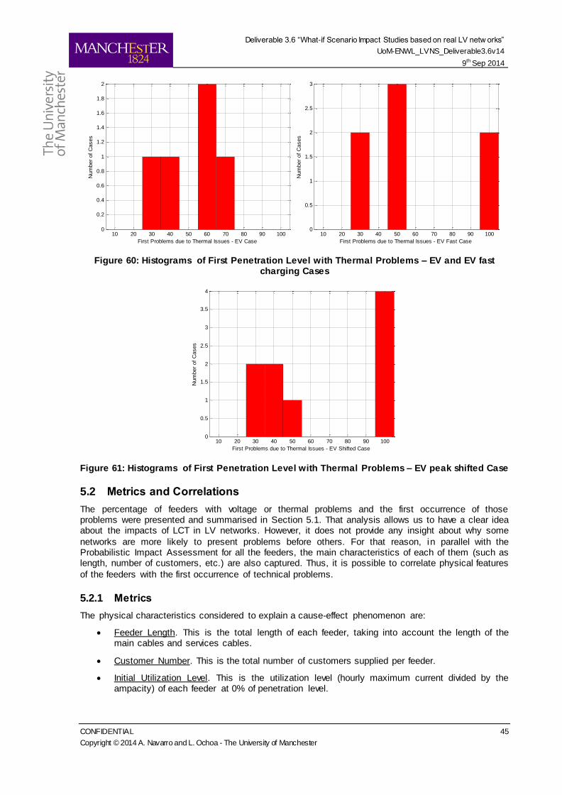
Deliverable 3.6 “What-if Scenario Impact Studies based on real LV netw orks”
UoM-ENWL_LVNS_Deliverable3.6v14
9th Sep 2014
CONFIDENTIAL 45
Copyright © 2014 A. Navarro and L. Ochoa - The University of Manchester
Figure 60: Histograms of First Penetration Level with Thermal Problems – EV and EV fast charging Cases
Figure 61: Histograms of First Penetration Level with Thermal Problems – EV peak shifted Case
5.2 Metrics and Correlations
The percentage of feeders with voltage or thermal problems and the first occurrence of those problems were presented and summarised in Section 5.1. That analysis allows us to have a clear idea about the impacts of LCT in LV networks. However, it does not provide any insight about why some
networks are more likely to present problems before others. For that reason, in parallel with the Probabilistic Impact Assessment for all the feeders, the main characteristics of each of them (such as length, number of customers, etc.) are also captured. Thus, it is possible to correlate physical features
of the feeders with the first occurrence of technical problems.
5.2.1 Metrics
The physical characteristics considered to explain a cause-effect phenomenon are:
Feeder Length. This is the total length of each feeder, taking into account the length of the main cables and services cables.
Customer Number. This is the total number of customers supplied per feeder.
Initial Utilization Level. This is the utilization level (hourly maximum current divided by the ampacity) of each feeder at 0% of penetration level.
10 20 30 40 50 60 70 80 90 1000
0.2
0.4
0.6
0.8
1
1.2
1.4
1.6
1.8
2
First Problems due to Thermal Issues - EV Case
Num
ber
of
Cases
10 20 30 40 50 60 70 80 90 1000
0.5
1
1.5
2
2.5
3
First Problems due to Thermal Issues - EV Fast Case
Num
ber
of
Cases
10 20 30 40 50 60 70 80 90 1000
0.5
1
1.5
2
2.5
3
3.5
4
First Problems due to Thermal Issues - EV Shifted Case
Num
ber
of
Cases
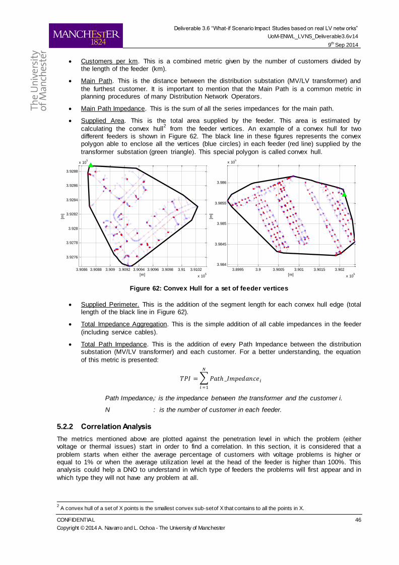
Deliverable 3.6 “What-if Scenario Impact Studies based on real LV netw orks”
UoM-ENWL_LVNS_Deliverable3.6v14
9th Sep 2014
CONFIDENTIAL 46
Copyright © 2014 A. Navarro and L. Ochoa - The University of Manchester
Customers per km. This is a combined metric given by the number of customers divided by the length of the feeder (km).
Main Path. This is the distance between the distribution substation (MV/LV transformer) and
the furthest customer. It is important to mention that the Main Path is a common metric in planning procedures of many Distribution Network Operators.
Main Path Impedance. This is the sum of all the series impedances for the main path.
Supplied Area. This is the total area supplied by the feeder. This area is estimated by
calculating the convex hull2 from the feeder vertices. An example of a convex hull for two
different feeders is shown in Figure 62. The black line in these figures represents the convex polygon able to enclose all the vertices (blue circles) in each feeder (red line) supplied by the
transformer substation (green triangle). This special polygon is called convex hull.
Figure 62: Convex Hull for a set of feeder vertices
Supplied Perimeter. This is the addition of the segment length for each convex hull edge (total length of the black line in Figure 62).
Total Impedance Aggregation. This is the simple addition of all cable impedances in the feeder
(including service cables).
Total Path Impedance. This is the addition of every Path Impedance between the distribution substation (MV/LV transformer) and each customer. For a better understanding, the equation
of this metric is presented:
∑
Path Impedancei: is the impedance between the transformer and the customer i.
N : is the number of customer in each feeder.
5.2.2 Correlation Analysis
The metrics mentioned above are plotted against the penetration level in which the problem (either voltage or thermal issues) start in order to find a correlation. In this section, it is considered that a
problem starts when either the average percentage of customers with voltage problems is higher or equal to 1% or when the average utilization level at the head of the feeder is higher than 100%. This analysis could help a DNO to understand in which type of feeders the problems will first appear and in
which type they will not have any problem at all.
2 A convex hull of a set of X points is the smallest convex sub-set of X that contains to all the points in X.
3.9086 3.9088 3.909 3.9092 3.9094 3.9096 3.9098 3.91 3.9102
x 105
3.9276
3.9278
3.928
3.9282
3.9284
3.9286
3.9288
x 105
[m]
[m]
3.8995 3.9 3.9005 3.901 3.9015 3.902
x 105
3.984
3.9845
3.985
3.9855
3.986
x 105
[m]
[m]
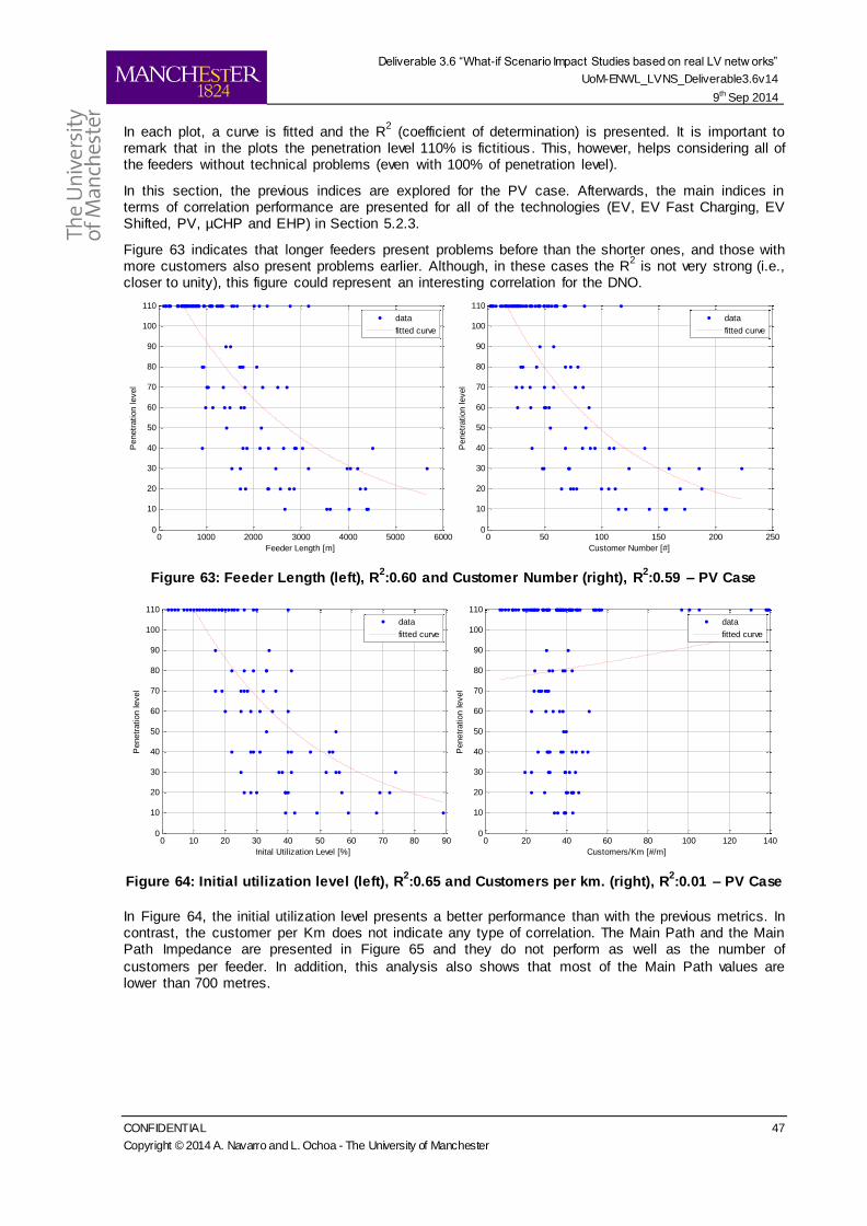
Deliverable 3.6 “What-if Scenario Impact Studies based on real LV netw orks”
UoM-ENWL_LVNS_Deliverable3.6v14
9th Sep 2014
CONFIDENTIAL 47
Copyright © 2014 A. Navarro and L. Ochoa - The University of Manchester
In each plot, a curve is fitted and the R2 (coefficient of determination) is presented. It is important to
remark that in the plots the penetration level 110% is fictitious. This, however, helps considering all of the feeders without technical problems (even with 100% of penetration level).
In this section, the previous indices are explored for the PV case. Afterwards, the main indices in terms of correlation performance are presented for all of the technologies (EV, EV Fast Charging, EV Shifted, PV, µCHP and EHP) in Section 5.2.3.
Figure 63 indicates that longer feeders present problems before than the shorter ones, and those with more customers also present problems earlier. Although, in these cases the R
2 is not very strong (i.e.,
closer to unity), this figure could represent an interesting correlation for the DNO.
Figure 63: Feeder Length (left), R2:0.60 and Customer Number (right), R
2:0.59 – PV Case
Figure 64: Initial utilization level (left), R2:0.65 and Customers per km. (right), R
2:0.01 – PV Case
In Figure 64, the initial utilization level presents a better performance than with the previous metrics. In contrast, the customer per Km does not indicate any type of correlation. The Main Path and the Main Path Impedance are presented in Figure 65 and they do not perform as well as the number of
customers per feeder. In addition, this analysis also shows that most of the Main Path values are lower than 700 metres.
0 1000 2000 3000 4000 5000 60000
10
20
30
40
50
60
70
80
90
100
110
Feeder Length [m]
Penetr
ation level
data
fitted curve
0 50 100 150 200 2500
10
20
30
40
50
60
70
80
90
100
110
Customer Number [#]
Penetr
ation level
data
fitted curve
0 10 20 30 40 50 60 70 80 900
10
20
30
40
50
60
70
80
90
100
110
Inital Utilization Level [%]
Penetr
ation level
data
fitted curve
0 20 40 60 80 100 120 1400
10
20
30
40
50
60
70
80
90
100
110
Customers/Km [#/m]
Penetr
ation level
data
fitted curve
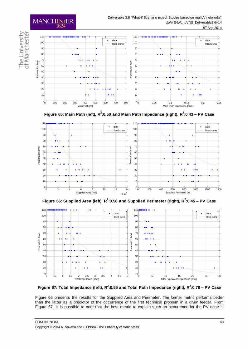
Deliverable 3.6 “What-if Scenario Impact Studies based on real LV netw orks”
UoM-ENWL_LVNS_Deliverable3.6v14
9th Sep 2014
CONFIDENTIAL 48
Copyright © 2014 A. Navarro and L. Ochoa - The University of Manchester
Figure 65: Main Path (left), R2:0.50 and Main Path Impedance (right), R
2:0.43 – PV Case
Figure 66: Supplied Area (left), R2:0.56 and Supplied Perimeter (right), R
2:0.45 – PV Case
Figure 67: Total Impedance (left), R2:0.55 and Total Path Impedance (right), R
2:0.78 – PV Case
Figure 66 presents the results for the Supplied Area and Perimeter. The former metric performs better than the latter as a predictor of the occurrence of the first technical problem in a given feeder. From Figure 67, it is possible to note that the best metric to explain such an occurrence for the PV case is
0 100 200 300 400 500 600 700 8000
10
20
30
40
50
60
70
80
90
100
110
Main Path [m]
Penetr
ation level
data
fitted curve
0 0.05 0.1 0.15 0.2 0.250
10
20
30
40
50
60
70
80
90
100
110
Main Path Impedance [ohm]
Penetr
ation level
data
fitted curve
0 2 4 6 8 10 12 14
x 104
0
10
20
30
40
50
60
70
80
90
100
110
Supplied Area [m2]
Penetr
ation level
data
fitted curve
0 200 400 600 800 1000 1200 14000
10
20
30
40
50
60
70
80
90
100
110
Supplied Perimeter [m]
Penetr
ation level
data
fitted curve
0 0.5 1 1.5 2 2.5 3 3.5 4 4.5 50
10
20
30
40
50
60
70
80
90
100
110
Total Impedance [ohm]
Penetr
ation level
data
fitted curve
0 5 10 15 20 25 300
10
20
30
40
50
60
70
80
90
100
110
Total Equivalent Impedance [ohm]
Penetr
ation level
data
fitted curve
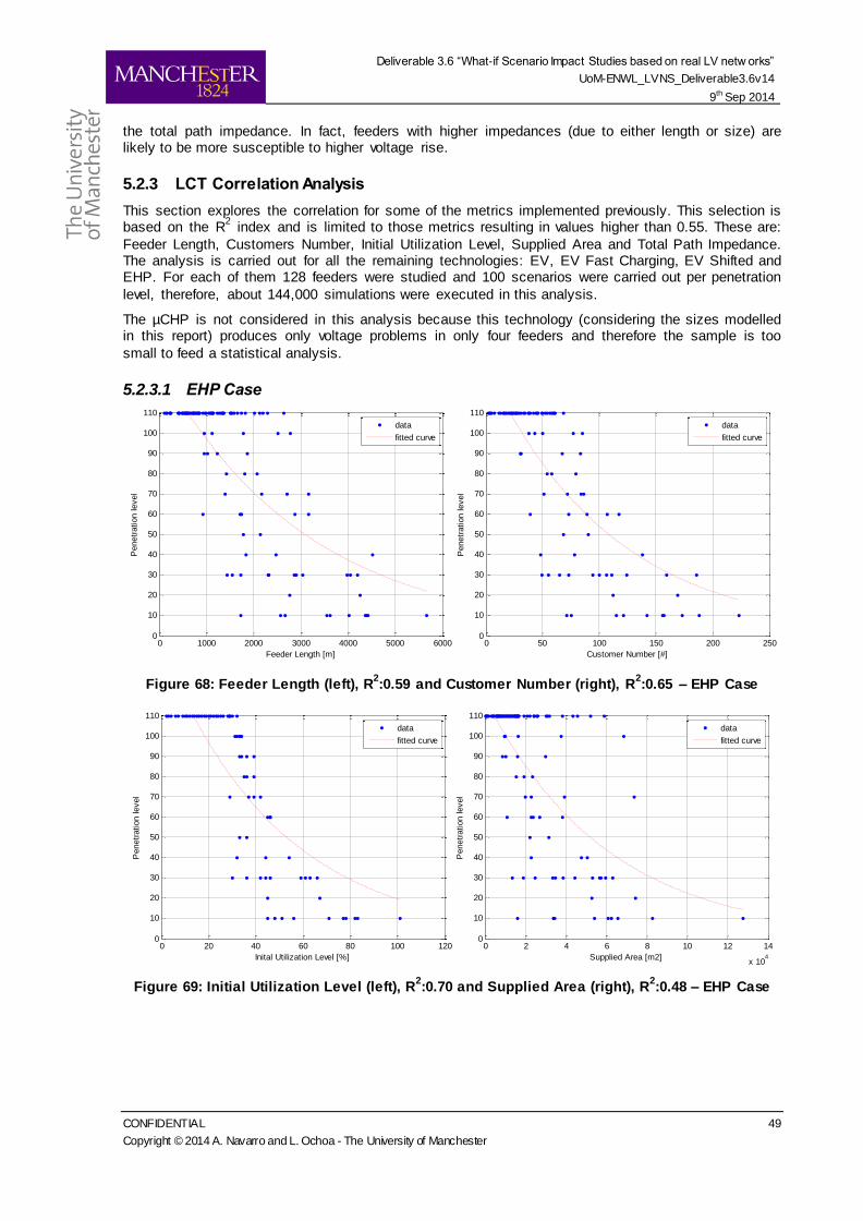
Deliverable 3.6 “What-if Scenario Impact Studies based on real LV netw orks”
UoM-ENWL_LVNS_Deliverable3.6v14
9th Sep 2014
CONFIDENTIAL 49
Copyright © 2014 A. Navarro and L. Ochoa - The University of Manchester
the total path impedance. In fact, feeders with higher impedances (due to either length or size) are likely to be more susceptible to higher voltage rise.
5.2.3 LCT Correlation Analysis
This section explores the correlation for some of the metrics implemented previously. This selection is based on the R
2 index and is limited to those metrics resulting in values higher than 0.55. These are:
Feeder Length, Customers Number, Initial Utilization Level, Supplied Area and Total Path Impedance. The analysis is carried out for all the remaining technologies: EV, EV Fast Charging, EV Shifted and EHP. For each of them 128 feeders were studied and 100 scenarios were carried out per penetration
level, therefore, about 144,000 simulations were executed in this analysis.
The µCHP is not considered in this analysis because this technology (considering the sizes modelled in this report) produces only voltage problems in only four feeders and therefore the sample is too
small to feed a statistical analysis.
5.2.3.1 EHP Case
Figure 68: Feeder Length (left), R2:0.59 and Customer Number (right), R
2:0.65 – EHP Case
Figure 69: Initial Utilization Level (left), R2:0.70 and Supplied Area (right), R
2:0.48 – EHP Case
0 1000 2000 3000 4000 5000 60000
10
20
30
40
50
60
70
80
90
100
110
Feeder Length [m]
Penetr
ation level
data
fitted curve
0 50 100 150 200 2500
10
20
30
40
50
60
70
80
90
100
110
Customer Number [#]
Penetr
ation level
data
fitted curve
0 20 40 60 80 100 1200
10
20
30
40
50
60
70
80
90
100
110
Inital Utilization Level [%]
Penetr
ation level
data
fitted curve
0 2 4 6 8 10 12 14
x 104
0
10
20
30
40
50
60
70
80
90
100
110
Supplied Area [m2]
Penetr
ation level
data
fitted curve
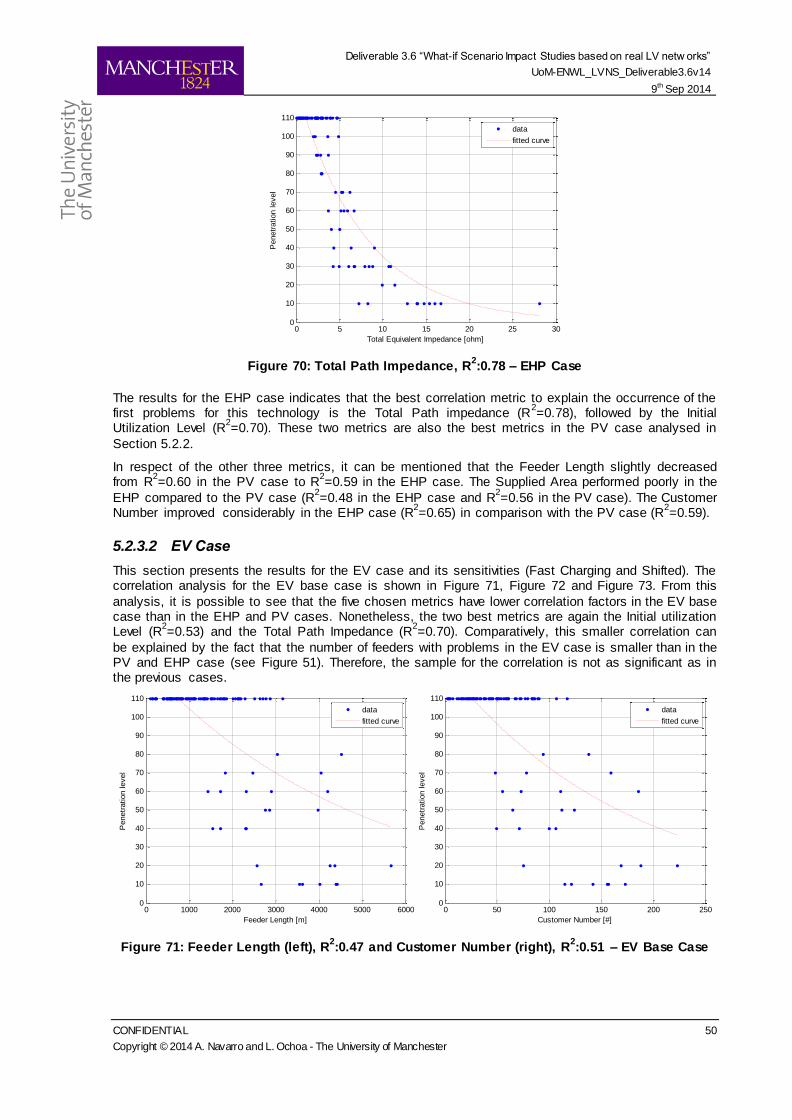
Deliverable 3.6 “What-if Scenario Impact Studies based on real LV netw orks”
UoM-ENWL_LVNS_Deliverable3.6v14
9th Sep 2014
CONFIDENTIAL 50
Copyright © 2014 A. Navarro and L. Ochoa - The University of Manchester
Figure 70: Total Path Impedance, R2:0.78 – EHP Case
The results for the EHP case indicates that the best correlation metric to explain the occurrence of the first problems for this technology is the Total Path impedance (R
2=0.78), followed by the Initial
Utilization Level (R2=0.70). These two metrics are also the best metrics in the PV case analysed in
Section 5.2.2.
In respect of the other three metrics, it can be mentioned that the Feeder Length slightly decreased from R
2=0.60 in the PV case to R
2=0.59 in the EHP case. The Supplied Area performed poorly in the
EHP compared to the PV case (R2=0.48 in the EHP case and R
2=0.56 in the PV case). The Customer
Number improved considerably in the EHP case (R2=0.65) in comparison with the PV case (R
2=0.59).
5.2.3.2 EV Case
This section presents the results for the EV case and its sensitivities (Fast Charging and Shifted). The correlation analysis for the EV base case is shown in Figure 71, Figure 72 and Figure 73. From this
analysis, it is possible to see that the five chosen metrics have lower correlation factors in the EV base case than in the EHP and PV cases. Nonetheless, the two best metrics are again the Initial utilization Level (R
2=0.53) and the Total Path Impedance (R
2=0.70). Comparatively, this smaller correlation can
be explained by the fact that the number of feeders with problems in the EV case is smaller than in the PV and EHP case (see Figure 51). Therefore, the sample for the correlation is not as significant as in the previous cases.
Figure 71: Feeder Length (left), R2:0.47 and Customer Number (right), R
2:0.51 – EV Base Case
0 5 10 15 20 25 300
10
20
30
40
50
60
70
80
90
100
110
Total Equivalent Impedance [ohm]
Penetr
ation level
data
fitted curve
0 1000 2000 3000 4000 5000 60000
10
20
30
40
50
60
70
80
90
100
110
Feeder Length [m]
Penetr
ation level
data
fitted curve
0 50 100 150 200 2500
10
20
30
40
50
60
70
80
90
100
110
Customer Number [#]
Penetr
ation level
data
fitted curve
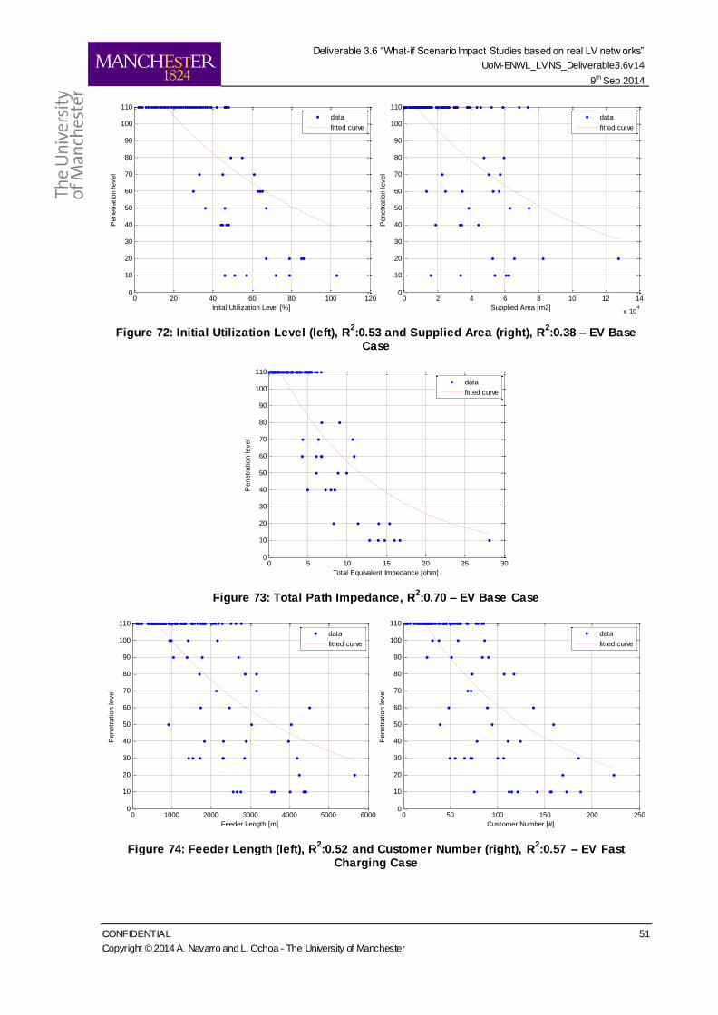
Deliverable 3.6 “What-if Scenario Impact Studies based on real LV netw orks”
UoM-ENWL_LVNS_Deliverable3.6v14
9th Sep 2014
CONFIDENTIAL 51
Copyright © 2014 A. Navarro and L. Ochoa - The University of Manchester
Figure 72: Initial Utilization Level (left), R2:0.53 and Supplied Area (right), R
2:0.38 – EV Base
Case
Figure 73: Total Path Impedance, R2:0.70 – EV Base Case
Figure 74: Feeder Length (left), R2:0.52 and Customer Number (right), R
2:0.57 – EV Fast
Charging Case
0 20 40 60 80 100 1200
10
20
30
40
50
60
70
80
90
100
110
Inital Utilization Level [%]
Penetr
ation level
data
fitted curve
0 2 4 6 8 10 12 14
x 104
0
10
20
30
40
50
60
70
80
90
100
110
Supplied Area [m2]
Penetr
ation level
data
fitted curve
0 5 10 15 20 25 300
10
20
30
40
50
60
70
80
90
100
110
Total Equivalent Impedance [ohm]
Penetr
ation level
data
fitted curve
0 1000 2000 3000 4000 5000 60000
10
20
30
40
50
60
70
80
90
100
110
Feeder Length [m]
Penetr
ation level
data
fitted curve
0 50 100 150 200 2500
10
20
30
40
50
60
70
80
90
100
110
Customer Number [#]
Penetr
ation level
data
fitted curve
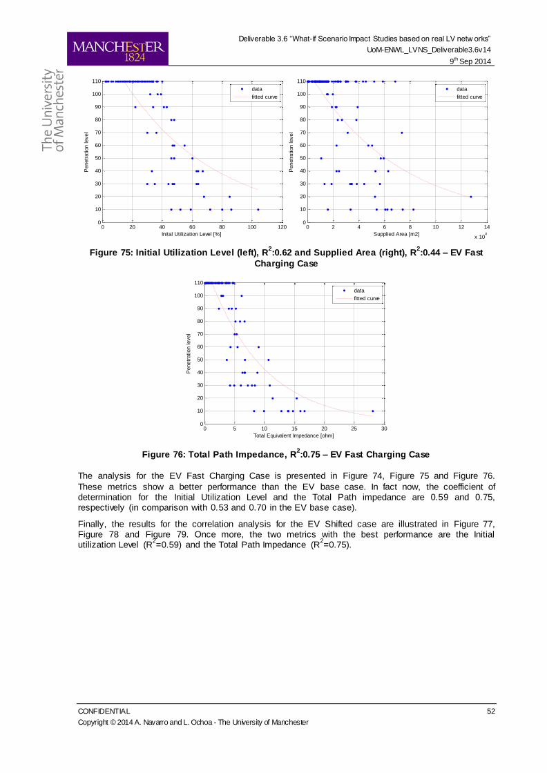
Deliverable 3.6 “What-if Scenario Impact Studies based on real LV netw orks”
UoM-ENWL_LVNS_Deliverable3.6v14
9th Sep 2014
CONFIDENTIAL 52
Copyright © 2014 A. Navarro and L. Ochoa - The University of Manchester
Figure 75: Initial Utilization Level (left), R2:0.62 and Supplied Area (right), R
2:0.44 – EV Fast
Charging Case
Figure 76: Total Path Impedance, R2:0.75 – EV Fast Charging Case
The analysis for the EV Fast Charging Case is presented in Figure 74, Figure 75 and Figure 76.
These metrics show a better performance than the EV base case. In fact now, the coefficient of determination for the Initial Utilization Level and the Total Path impedance are 0.59 and 0.75, respectively (in comparison with 0.53 and 0.70 in the EV base case).
Finally, the results for the correlation analysis for the EV Shifted case are illustrated in Figure 77, Figure 78 and Figure 79. Once more, the two metrics with the best performance are the Initial utilization Level (R
2=0.59) and the Total Path Impedance (R
2=0.75).
0 20 40 60 80 100 1200
10
20
30
40
50
60
70
80
90
100
110
Inital Utilization Level [%]
Penetr
ation level
data
fitted curve
0 2 4 6 8 10 12 14
x 104
0
10
20
30
40
50
60
70
80
90
100
110
Supplied Area [m2]
Penetr
ation level
data
fitted curve
0 5 10 15 20 25 300
10
20
30
40
50
60
70
80
90
100
110
Total Equivalent Impedance [ohm]
Penetr
ation level
data
fitted curve

Deliverable 3.6 “What-if Scenario Impact Studies based on real LV netw orks”
UoM-ENWL_LVNS_Deliverable3.6v14
9th Sep 2014
CONFIDENTIAL 53
Copyright © 2014 A. Navarro and L. Ochoa - The University of Manchester
Figure 77: Feeder Length (left), R2:0.52 and Customer Number (right), R
2:0.58 – EV Shifted Case
Figure 78: Initial Utilization Level (left), R2:0.59 and Supplied Area (right), R
2:0.42 – EV Shifted
Case
Figure 79: Total Path Impedance, R2:0.75 – EV Shifted Case
0 1000 2000 3000 4000 5000 60000
10
20
30
40
50
60
70
80
90
100
110
Feeder Length [m]
Penetr
ation level
data
fitted curve
0 50 100 150 200 2500
10
20
30
40
50
60
70
80
90
100
110
Customer Number [#]
Penetr
ation level
data
fitted curve
0 20 40 60 80 100 1200
10
20
30
40
50
60
70
80
90
100
110
Inital Utilization Level [%]
Penetr
ation level
data
fitted curve
0 2 4 6 8 10 12 14
x 104
0
10
20
30
40
50
60
70
80
90
100
110
Supplied Area [m2]
Penetr
ation level
data
fitted curve
0 5 10 15 20 25 300
10
20
30
40
50
60
70
80
90
100
110
Total Equivalent Impedance [ohm]
Penetr
ation level
data
fitted curve
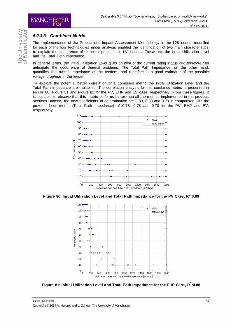
Deliverable 3.6 “What-if Scenario Impact Studies based on real LV netw orks”
UoM-ENWL_LVNS_Deliverable3.6v14
9th Sep 2014
CONFIDENTIAL 54
Copyright © 2014 A. Navarro and L. Ochoa - The University of Manchester
5.2.3.3 Combined Metric
The implementation of the Probabilistic Impact Assessment Methodology in the 128 feeders modelled
for each of the four technologies under analysis enabled the identification of two main characteristics to explain the occurrence of technical problems in LV feeders. These are: the Initial Utilization Level and the Total Path Impedance.
In general terms, the Initial Utilization Level gives an idea of the current rating status and therefore can anticipate the occurrence of thermal problems. The Total Path Impedance, on the other hand, quantifies the overall impedance of the feeders, and therefore is a good estimator of the possible
voltage drop/rise in the feeder.
To explore the potential better correlation of a combined metric the Initial Utilization Level and the Total Path impedance are multiplied. The correlation analysis for this combined metric is presented in
Figure 80, Figure 81 and Figure 82 for the PV, EHP and EV case, respectively. From these figures, it is possible to observe that this metric performs better than all the metrics implemented in the previous sections. Indeed, the new coefficients of determination are 0.80, 0.88 and 0.79 in comparison with the
previous best metric (Total Path Impedance) of 0.78, 0.78 and 0.70 for the PV, EHP and EV, respectively.
Figure 80: Initial Utilization Level and Total Path Impedance for the PV Case, R2:0.80
Figure 81: Initial Utilization Level and Total Path Impedance for the EHP Case, R2:0.88
0 200 400 600 800 1000 1200 1400 1600 18000
10
20
30
40
50
60
70
80
90
100
110
Utilization Level and Total Path Impedance [%*ohm]
Penetr
ation level
data
fitted curve
0 200 400 600 800 1000 1200 1400 1600 1800 20000
10
20
30
40
50
60
70
80
90
100
110
Utilization Level and Total Path Impedance [%*ohm]
Penetr
ation level
data
fitted curve
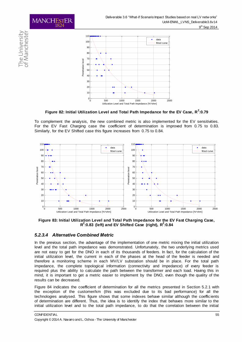
Deliverable 3.6 “What-if Scenario Impact Studies based on real LV netw orks”
UoM-ENWL_LVNS_Deliverable3.6v14
9th Sep 2014
CONFIDENTIAL 55
Copyright © 2014 A. Navarro and L. Ochoa - The University of Manchester
Figure 82: Initial Utilization Level and Total Path Impedance for the EV Case, R2:0.79
To complement the analysis, the new combined metric is also implemented for the EV sensitivities. For the EV Fast Charging case the coefficient of determination is improved from 0.75 to 0.83.
Similarly, for the EV Shifted case this figure increases from 0.75 to 0.84.
Figure 83: Initial Utilization Level and Total Path Impedance for the EV Fast Charging Case, R
2:0.83 (left) and EV Shifted Case (right), R
2:0.84
5.2.3.4 Alternative Combined Metric
In the previous section, the advantage of the implementation of one metric mixing the initial utilization level and the total path impedance was demonstrated. Unfortunately, the two underlying metrics used
are not easy to get for the DNO in each of its thousands of feeders. In fact, for the calculation of the initial utilization level, the current in each of the phases at the head of the feeder is needed and therefore a monitoring scheme in each MV/LV substation should be in place. For the total path
impedance, the complete topological information (connectivity and impedance) of every feeder is required plus the ability to calculate the path between the transformer and each load. Having this in mind, it is important to get a metric easier to implement by the DNO, even though the quality of the
results can be decreased.
Figure 84 indicates the coefficient of determination for all the metrics presented in Section 5.2.1 with the exception of the customer/km (this was excluded due to its bad performance) for all the
technologies analysed. This figure shows that some indexes behave similar although the coeffic ients of determination are different. Thus, the idea is to identify the index that behaves more similar to the initial utilization level and to the total path impedance, to do that the correlation between the initial
0 500 1000 1500 2000 25000
10
20
30
40
50
60
70
80
90
100
110
Utilization Level and Total Path Impedance [%*ohm]
Penetr
ation level
data
fitted curve
0 500 1000 1500 2000 25000
10
20
30
40
50
60
70
80
90
100
110
Utilization Level and Total Path Impedance [%*ohm]
Penetr
ation level
data
fitted curve
0 500 1000 1500 2000 25000
10
20
30
40
50
60
70
80
90
100
110
Utilization Level and Total Path Impedance [%*ohm]
Penetr
ation level
data
fitted curve
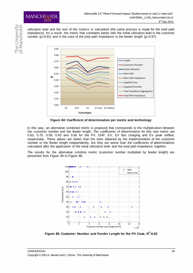
Deliverable 3.6 “What-if Scenario Impact Studies based on real LV netw orks”
UoM-ENWL_LVNS_Deliverable3.6v14
9th Sep 2014
CONFIDENTIAL 56
Copyright © 2014 A. Navarro and L. Ochoa - The University of Manchester
utilization level and the rest of the metrics is calculated (the same process is made for the total path impedance). As a result, the metric that correlates better with the initial utilization level is the customer number (ρ=0.91) and in the case of the total path impedance is the feeder length (ρ=0.97).
Figure 84: Coefficient of determination per metric and technology
In this way, an alternative combined metric is proposed that corresponds to the multiplication between the customer number and the feeder length. The coefficients of determination for this new metric are 0.63, 0.70, 0.59, 0.63 and 0.66 for the PV, EHP, EV, EV fast charging and EV peak shifted,
respectively. These values are better than the ones obtained by the implementation of the customer number or the feeder length independently, but they are worse than the coefficients of determinations calculated after the application of the initial utilization level and the total path impedance together.
The results for the alternative combine metric (customer number multiplied by feeder length) are presented from Figure 85 to Figure 88.
Figure 85: Customer Number and Feeder Length for the PV Case, R2:0.63
0.00
0.10
0.20
0.30
0.40
0.50
0.60
0.70
0.80
0.90
PV EHP EV EV Fast EV Shifted
R2
Technologies
Length
Customers Number
Initial Utilization
Main Path
Main Path Impedance
Supplied Area
Supplied Perimiter
Total Impedance Aggregation
Total Path Impedance
0 2 4 6 8 10 12 14
x 105
0
10
20
30
40
50
60
70
80
90
100
110
Custumer Number and Length [%*m]
Penetr
ation level
data
fitted curve
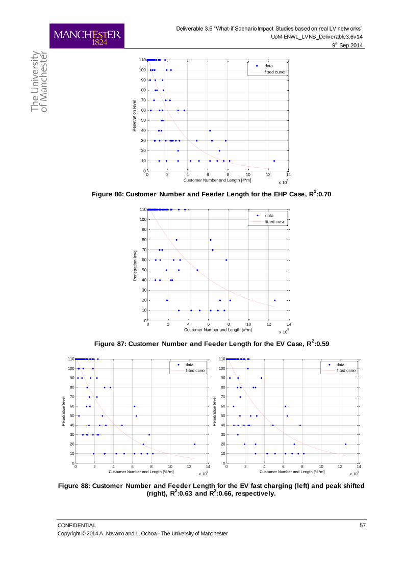
Deliverable 3.6 “What-if Scenario Impact Studies based on real LV netw orks”
UoM-ENWL_LVNS_Deliverable3.6v14
9th Sep 2014
CONFIDENTIAL 57
Copyright © 2014 A. Navarro and L. Ochoa - The University of Manchester
Figure 86: Customer Number and Feeder Length for the EHP Case, R2:0.70
Figure 87: Customer Number and Feeder Length for the EV Case, R2:0.59
Figure 88: Customer Number and Feeder Length for the EV fast charging (left) and peak shifted (right), R
2:0.63 and R
2:0.66, respectively.
0 2 4 6 8 10 12 14
x 105
0
10
20
30
40
50
60
70
80
90
100
110
Customer Number and Length [#*m]
Penetr
ation level
data
fitted curve
0 2 4 6 8 10 12 14
x 105
0
10
20
30
40
50
60
70
80
90
100
110
Customer Number and Length [#*m]
Penetr
ation level
data
fitted curve
0 2 4 6 8 10 12 14
x 105
0
10
20
30
40
50
60
70
80
90
100
110
Custumer Number and Length [%*m]
Penetr
ation level
data
fitted curve
0 2 4 6 8 10 12 14
x 105
0
10
20
30
40
50
60
70
80
90
100
110
Custumer Number and Length [%*m]
Penetr
ation level
data
fitted curve
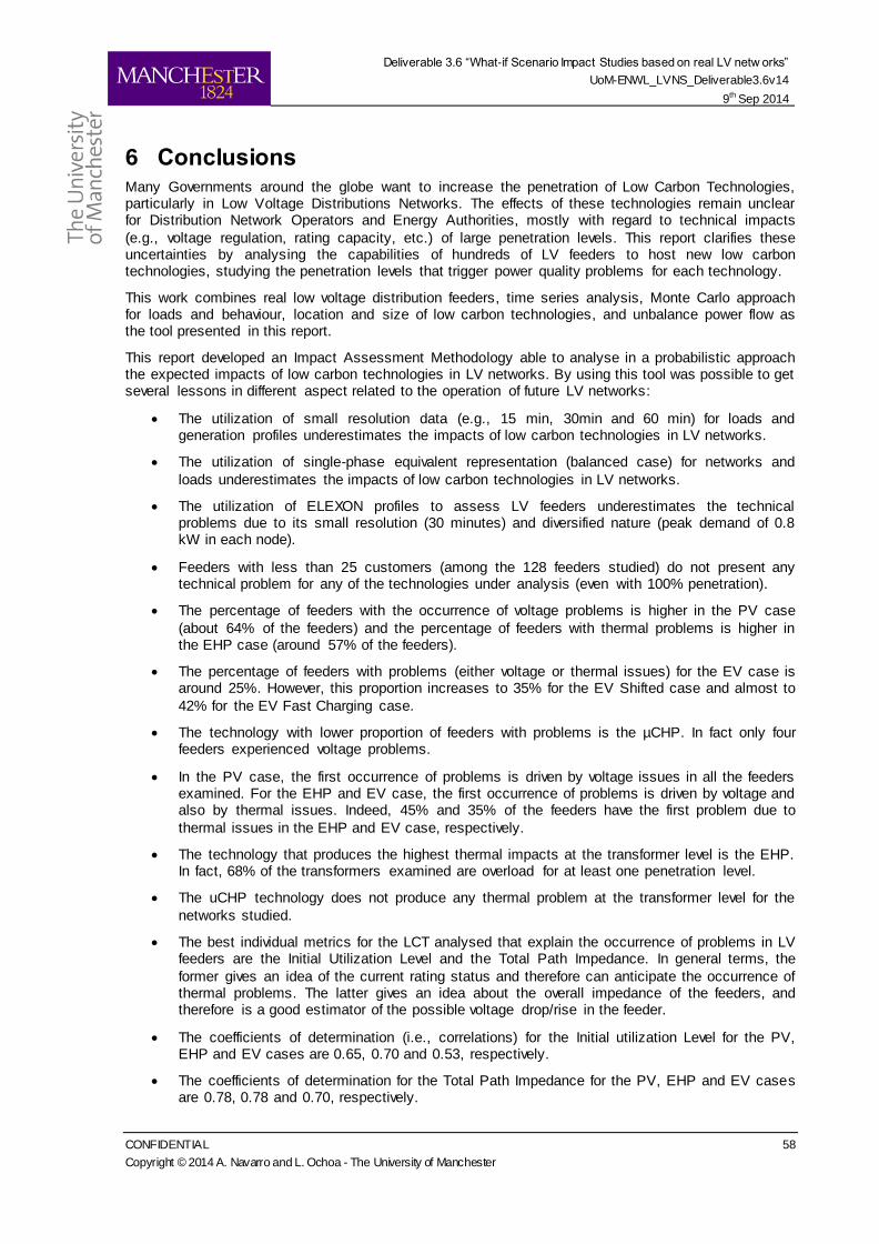
Deliverable 3.6 “What-if Scenario Impact Studies based on real LV netw orks”
UoM-ENWL_LVNS_Deliverable3.6v14
9th Sep 2014
CONFIDENTIAL 58
Copyright © 2014 A. Navarro and L. Ochoa - The University of Manchester
6 Conclusions Many Governments around the globe want to increase the penetration of Low Carbon Technologies, particularly in Low Voltage Distributions Networks. The effects of these technologies remain unclear for Distribution Network Operators and Energy Authorities, mostly with regard to technical impacts
(e.g., voltage regulation, rating capacity, etc.) of large penetration levels. This report clarifies these uncertainties by analysing the capabilities of hundreds of LV feeders to host new low carbon technologies, studying the penetration levels that trigger power quality problems for each technology.
This work combines real low voltage distribution feeders, time series analysis, Monte Carlo approach for loads and behaviour, location and size of low carbon technologies, and unbalance power flow as the tool presented in this report.
This report developed an Impact Assessment Methodology able to analyse in a probabilistic approach the expected impacts of low carbon technologies in LV networks. By using this tool was possible to get several lessons in different aspect related to the operation of future LV networks:
The utilization of small resolution data (e.g., 15 min, 30min and 60 min) for loads and generation profiles underestimates the impacts of low carbon technologies in LV networks.
The utilization of single-phase equivalent representation (balanced case) for networks and
loads underestimates the impacts of low carbon technologies in LV networks.
The utilization of ELEXON profiles to assess LV feeders underestimates the technical problems due to its small resolution (30 minutes) and diversified nature (peak demand of 0.8 kW in each node).
Feeders with less than 25 customers (among the 128 feeders studied) do not present any technical problem for any of the technologies under analysis (even with 100% penetration).
The percentage of feeders with the occurrence of voltage problems is higher in the PV case
(about 64% of the feeders) and the percentage of feeders with thermal problems is higher in the EHP case (around 57% of the feeders).
The percentage of feeders with problems (either voltage or thermal issues) for the EV case is around 25%. However, this proportion increases to 35% for the EV Shifted case and almost to
42% for the EV Fast Charging case.
The technology with lower proportion of feeders with problems is the µCHP. In fact only four feeders experienced voltage problems.
In the PV case, the first occurrence of problems is driven by voltage issues in all the feeders examined. For the EHP and EV case, the first occurrence of problems is driven by voltage and also by thermal issues. Indeed, 45% and 35% of the feeders have the first problem due to
thermal issues in the EHP and EV case, respectively.
The technology that produces the highest thermal impacts at the transformer level is the EHP. In fact, 68% of the transformers examined are overload for at least one penetration level.
The uCHP technology does not produce any thermal problem at the transformer level for the
networks studied.
The best individual metrics for the LCT analysed that explain the occurrence of problems in LV feeders are the Initial Utilization Level and the Total Path Impedance. In general terms, the
former gives an idea of the current rating status and therefore can anticipate the occurrence of thermal problems. The latter gives an idea about the overall impedance of the feeders, and therefore is a good estimator of the possible voltage drop/rise in the feeder.
The coefficients of determination (i.e., correlations) for the Initial utilization Level for the PV, EHP and EV cases are 0.65, 0.70 and 0.53, respectively.
The coefficients of determination for the Total Path Impedance for the PV, EHP and EV cases are 0.78, 0.78 and 0.70, respectively.

Deliverable 3.6 “What-if Scenario Impact Studies based on real LV netw orks”
UoM-ENWL_LVNS_Deliverable3.6v14
9th Sep 2014
CONFIDENTIAL 59
Copyright © 2014 A. Navarro and L. Ochoa - The University of Manchester
The combination of the Initial Utilization Level and the Total Path Impedance increases the coefficient of determination for all the technologies. In fact, the multiplication of these two metrics produces coefficients of determination equal to 0.80, 0.88 and 0.79 for the PV, EHP
and EV cases, respectively.
Due to it is highly likely that the DNOs cannot introduce in the short term the combine metric proposed, an alternative metric was developed as a proxy. This metric is the multiplication
between the number of customers and the feeder length.
Finally, it is important to remark that with the methodology implemented, the DNO can analyse the potential risk (in terms of probabilities) of having certain low carbon technology penetration in their
networks.
It is important to highlight that this document (version 14, September 2014) corresponds to an updated version of the Deliverable 3.6 “What-if Scenario Impact Studies based on real LV networks” produced
in May 2014 which was used for the project’s Close Down report. This updated version considers summer load profiles for the PV cases. The corresponding updated analysis did not result in any significant difference in the conclusions presented in this report or the Close Down report.
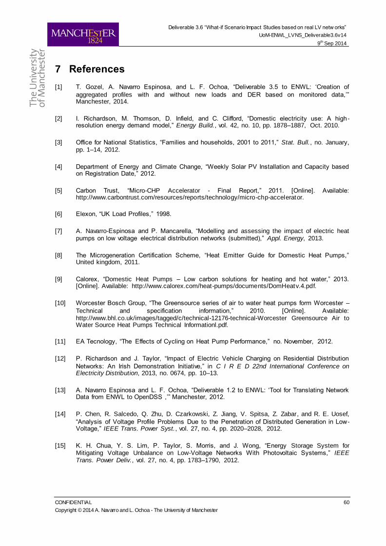
Deliverable 3.6 “What-if Scenario Impact Studies based on real LV netw orks”
UoM-ENWL_LVNS_Deliverable3.6v14
9th Sep 2014
CONFIDENTIAL 60
Copyright © 2014 A. Navarro and L. Ochoa - The University of Manchester
7 References
[1] T. Gozel, A. Navarro Espinosa, and L. F. Ochoa, “Deliverable 3.5 to ENWL: ‘Creation of
aggregated profiles with and without new loads and DER based on monitored data,’” Manchester, 2014.
[2] I. Richardson, M. Thomson, D. Infield, and C. Clifford, “Domestic electricity use: A high-resolution energy demand model,” Energy Build., vol. 42, no. 10, pp. 1878–1887, Oct. 2010.
[3] Office for National Statistics, “Families and households, 2001 to 2011,” Stat. Bull., no. January, pp. 1–14, 2012.
[4] Department of Energy and Climate Change, “Weekly Solar PV Installation and Capacity based on Registration Date,” 2012.
[5] Carbon Trust, “Micro-CHP Accelerator - Final Report,” 2011. [Online]. Available: http://www.carbontrust.com/resources/reports/technology/micro-chp-accelerator.
[6] Elexon, “UK Load Profiles,” 1998.
[7] A. Navarro-Espinosa and P. Mancarella, “Modelling and assessing the impact of electric heat pumps on low voltage electrical distribution networks (submitted),” Appl. Energy, 2013.
[8] The Microgeneration Certification Scheme, “Heat Emitter Guide for Domestic Heat Pumps,” United kingdom, 2011.
[9] Calorex, “Domestic Heat Pumps – Low carbon solutions for heating and hot water,” 2013. [Online]. Available: http://www.calorex.com/heat-pumps/documents/DomHeatv.4.pdf.
[10] Worcester Bosch Group, “The Greensource series of air to water heat pumps form Worcester –
Technical and specification information,” 2010. [Online]. Available: http://www.bhl.co.uk/images/tagged/c/technical-12176-technical-Worcester Greensource Air to Water Source Heat Pumps Technical Informationl.pdf.
[11] EA Tecnology, “The Effects of Cycling on Heat Pump Performance,” no. November, 2012.
[12] P. Richardson and J. Taylor, “Impact of Electric Vehicle Charging on Residential Distribution
Networks: An Irish Demonstration Initiative,” in C I R E D 22nd International Conference on Electricity Distribution, 2013, no. 0674, pp. 10–13.
[13] A. Navarro Espinosa and L. F. Ochoa, “Deliverable 1.2 to ENWL: ‘Tool for Translating Network Data from ENWL to OpenDSS ,’” Manchester, 2012.
[14] P. Chen, R. Salcedo, Q. Zhu, D. Czarkowski, Z. Jiang, V. Spitsa, Z. Zabar, and R. E. Uosef,
“Analysis of Voltage Profile Problems Due to the Penetration of Distributed Generation in Low-Voltage,” IEEE Trans. Power Syst., vol. 27, no. 4, pp. 2020–2028, 2012.
[15] K. H. Chua, Y. S. Lim, P. Taylor, S. Morris, and J. Wong, “Energy Storage System for Mitigating Voltage Unbalance on Low-Voltage Networks With Photovoltaic Systems,” IEEE Trans. Power Deliv., vol. 27, no. 4, pp. 1783–1790, 2012.
Deliverable 3.6 “What-if Scenario Impact Studies based on real LV netw orks”
UoM-ENWL_LVNS_Deliverable3.6v14
9th Sep 2014
CONFIDENTIAL 61
Copyright © 2014 A. Navarro and L. Ochoa - The University of Manchester
[16] F. Demailly, O. Ninet, and A. Even, “Numerical Tools and Models for Monte Carlo Studies of the Influence on Embedded Generation on Voltage Limits in LV Grids,” IEEE Trans. Power Syst., vol. 20, no. 3, pp. 2343–2350, 2005.
[17] R. A. Shayani and M. aurelio Gonçalves De Oliveira, “Photovoltaic Generation Penetration
Limits in Radial Distribution Systems,” IEEE Trans. Power Syst., vol. 26, no. 3, pp. 1625–1631, 2011.
[18] R. Tonkoski, D. Turcotte, and T. H. M. El-Fouly, “Impact of High PV Penetration on Voltage Profiles in Residential Neighborhoods,” IEEE Trans. Sustain. Energy, vol. 3, no. 3, pp. 518–527, Jul. 2012.
[19] A. Hoke, R. Butler, J. Hambrick, and B. Kroposki, “Steady -State Analysis of Maximum Photovoltaic Penetration Levels on Typical Distribution Feeders,” IEEE Trans. Sustain. Energy, vol. 4, no. 2, pp. 350–357, 2013.
[20] A. Navarro, L. F. Ochoa, and D. Randles, “Monte Carlo-Based Assessment of PV Impacts on
Real UK Low Voltage Networks,” in 2013 IEEE Power and Energy Society General Meeting, 2013, pp. 1–5.
[21] A. Navarro-Espinosa, L. F. Ochoa, P. Mamcarella, and D. Randles, “Impacts of Photovoltaics on Low voltage Networks: A Case Study for the North West of England,” in 22th International Conference on electricity Distribution (CIRED 2013), 2013, no. June, pp. 10–13.
[22] Brisitsh Standards Institution, “BS EN 50160: Voltage characteristics of electricity supplied by public distribution systems,” 2000.
[23] Electricity North West Limited, “Code of Practice 226: Low Voltage Network Design,” 2011.