Delegated Decision-Making in Finance

Felix Holzmeister, Martin Holmén, Michael Kirchler, MatthiasStefan, Erik Wengström

Working Papers in Economics and Statistics

����-��

University of Innsbruckhttps://www.uibk.ac.at/eeecon/

University of InnsbruckWorking Papers in Economics and Statistics

The series is jointly edited and published by

- Department of Banking and Finance

- Department of Economics

- Department of Public Finance

- Department of Statistics

Contact address of the editor:research platform “Empirical and Experimental Economics”University of InnsbruckUniversitaetsstrasse ��A-���� InnsbruckAustriaTel: + �� ��� ��� �����Fax: + �� ��� ��� ����E-mail: eeecon@uibk.ac.at

The most recent version of all working papers can be downloaded athttps://www.uibk.ac.at/eeecon/wopec/

For a list of recent papers see the backpages of this paper.

Delegated Decision-Making in Finance

Felix Holzmeister† Martin Holmén‡,ú Michael Kirchler†,‡

Matthias Stefan† Erik Wengström§,¶

† University of Innsbruck, Department of Banking and Finance‡ University of Gothenburg, Department of Economics, Centre for Finance

§ Lund University, Department of Economics¶ Hanken School of Economics, Department of Finance and Economics

ú Corresponding author: martin.holmen@gu.se

Abstract

We run an online experiment with 408 �nance professionals (money managers) and 550subjects from the general population in Sweden (clients). We examine drivers of clients’delegation decisions, di�erences in decision-making quality between both groups, andprofessionals’ ability to implement investment portfolios that suit the clients’ risk atti-tudes. We �nd that clients’ trust in money managers increases the likelihood of dele-gating their investment decisions, whereas decision-making quality is associated with adecrease. We further show that decision-making quality of �nance professionals is notsigni�cantly higher compared to their clients’ when controlling for risk taking. Finally,we observe high variability among professionals’ perception of delegated risk levels andoverlaps in portfolio risk across self-reported risk-levels of clients. This �nding indi-cates that communicating risk between clients and professionals constitutes a potentialpitfall in delegated investment decisions.

JEL: C93, G11, G41.Keywords: Experimental �nance, �nance professionals, delegated decision-making.

We thank Pol Campos-Mercade, Alain Cohn, Dawei Fang, Christian König-Kersting, Michael Razen, Markus Walzl, seminarparticipants at the Berlin Behavioral Economics Colloquium and Seminar, the Helsinki GSE Colloquium, as well as conferenceparticipants of the Organizations and Society Workshop 2019 at the University of Innsbruck, the NOeG 2019 (Austrian Eco-nomic Association) in Graz, the SFB Workshop 2019 in Innsbruck, the Experimental Finance Conference 2019 in Copenhagen,the Decision-Making for Others Workshop in Nijmegen 2018, and the Workshop on Trust and Cooperation in Markets and Or-ganizations in Stavanger 2019 for very valuable comments. We particularly thank Fredrik Bergdahl at Statistiska centralbyrån forthe excellent collaboration on the project. Financial support from the Austrian Science Fund FWF (START-grant Y617-G11 andSFB F63), and the Swedish Research Council (grant 2015-01713) is gratefully acknowledged. This study was ethically approvedby the review boards at Statistiska centralbyrån (SCB; Statistics Sweden) and in Gothenburg (Sweden).

1. Introduction

Given the complexity of �nancial products andmarkets, private investors often opt for delegating decisionsto �nance professionals. This involves decisions about portfolio investments, insurance and pension plans,and seeking advice on various other �nancial aspects, all of which have a potentially strong impact on aclient’s wealth. The economic importance of delegated decision-making in �nance is indicated by thelarge and growing market for �nancial advice and decision-making on behalf of clients. For instance, in2017, the net asset value of US mutual funds equaled 18.8 trillion USD1, and over 271,000 professionalswere employed as personal �nancial advisors in the United States2. Thus, it is surprising that research ineconomics and �nance has predominantly focused on individual decision-making (e.g., Holt and Laury,2002; Abdellaoui et al., 2011; Dohmen et al., 2011; Falk et al., 2018) without giving much considerationto how delegation decisions by clients and delegated investment decisions by �nance professionals areactually taken (as emphasized by, e.g., Foerster et al., 2017; Kirchler et al., 2018a; Linnainmaa et al., 2019).

We study delegation decisions by laypeople and how �nance professionals behave on their behalf by run-ning a controlled lab-in-the �eld experiment implemented online with �nance professionals (agents) andsubjects from the general population (principals) in Sweden. We examine (i) the motivations and charac-teristics of principals delegating investment decisions, (ii) di�erences in decision-making quality betweenprofessionals and the general population, and (iii) the agents’ ability to construct portfolios that suit therisk preferences of principals.

The reasons why private (and, partly, also institutional) investors delegate investment decisions to pro-fessional money managers (e.g., �nancial advisers or fund managers) are not well understood. Straight-forward potential explanations include that investors lack—or believe to lack—su�cient knowledge orinformation, or are time-constrained. An alternative motive for delegating investments may be the pos-sibility to blame the agent if the investment does not turn out as expected (Shefrin, 2007; Chang et al.,2016).3 Moreover, Gennaioli et al. (2015) argue that investors delegate because they do not know muchabout �nance and are too anxious to make investment decisions. Just like doctors, money managers aretrusted, and they give investors con�dence to take risks (see also Guiso et al., 2004, 2008, for the “trustchannel” as a major motive of delegated investment decisions). In their theoretical framework Gennaioliet al. (2015) show that, under rational expectations, money managers enable investors to take more riskand, consequently, being better o�.

However, since the seminal work of Jensen (1968) there is clear and persistent evidence that fundmanagersunderperform passive benchmark indices after costs. The annual underperformance varies and mainlyfalls within the range of 0.6 and 2.0 percent (see, for instance, Gruber, 1996; Carhart, 1997; French, 2008).This insight renders the question of why people delegate their �nancial decisions more puzzling. More-over, money managers have a strong incentive not to correct investors’ biased beliefs, because they enablecharging higher fees (Mullainathan et al., 2012). This �nding is also related to the credence goods char-acteristics of �nancial advice (Dulleck and Kerschbamer, 2006; Inderst and Ottaviani, 2012a,b,c), outliningthe prevailing information asymmetry between advisers and clients.

1 https://perma.cc/5VUB-U98U2 https://perma.cc/5RYT-CP6H3 For a general account of shifting blame see also Bartling and Fischbacher (2012).

2

In addition, not only asymmetric information, but also monetary incentives of �nancial professionals andtheir role of intensifying con�icts of interest between clients and money managers are relevant in dele-gating �nancial investment decisions. Payment schemes have become a hotly debated topic in �nance,as misaligned incentives have been portrayed as major contributors to the last �nancial crisis (FinancialCrisis Inquiry Commission, 2011; Dewatripont and Freixas, 2012). In particular, high-powered paymentschemes that align professionals’ incentives with clients’ returns (e.g., bonus schemes or tournament in-centives) have been identi�ed among the main drivers of excessive risk taking in �nancial markets (Jensenand Meckling, 1976; Rajan, 2006; Diamond and Rajan, 2009; Bebchuk and Spamann, 2010). Since thisdebate—in particular on bonus incentives—has spilled over to the public, incentives might also play a rolefor decisions whether to delegate.

A growing strand of literature uses experiments with student or general population samples to examinerisk taking in delegated decision-making. Several studies report a “risky shift” in risk-taking, indicatingthat decision-makers take more risks or show less loss-averse behavior for others than for themselves (e.g.,Sutter, 2009; Chakravarty et al., 2011; Andersson et al., 2016; Vieider et al., 2016). However, a substantialnumber of studies also �nd a “cautious shift” when the money of third parties is invested (Bolton andOckenfels, 2010; Eriksen and Kvaløy, 2010)—see Füllbrunn and Luhan (2015) and Eriksen et al. (2017)for overviews. Andersson et al. (2019) run a large-scale study with a random population sample fromDenmark. The agents face high-powered incentives to increase risk-taking on behalf of others throughhedged compensation contracts or tournament incentives. The authors report that the decision-makersrespond to these incentives, resulting in an increased risk exposure of the principals. Yet another strand ofexperimental studies suggests that even strong �nancial incentives hardly interfere with agents’ attemptto adhere to their clients’ preferences (see, e.g., Rud et al., 2018; Ifcher and Zarghamee, 2019; Kling et al.,2019).

In recent years, robo advice and algorithm-based investments have emerged as an alternative to traditional�nancial services. Although they promise to o�er a�ordable advice in investment matters, tailored to theclients’ needs, several pitfalls remain (D’Acunto et al., 2019). Similar to the case of delegating to �nancialprofessionals, the decision to opt for robo advice is likely shaped by trust. Previous research from otherdecision domains provides evidence of algorithm aversion, with people distrusting advice and predictionsbased on algorithms more than those based on human judgement (Dietvorst et al., 2014; Harvey et al.,2017; Longoni et al., 2019). However, the evidence is mixed, and other studies report the opposite patternof algorithm appreciation (Logg et al., 2017). To date, there is a lack of evidence on this issue in the realmof �nancial decision-making.

Given that �nance professionals regularly make decisions on behalf of their clients and that there is a lackof knowledge regarding the motives for delegation among laypeople, it is surprising that no evidence onprofessionals’ �duciary and clients’ delegation choices exists. In this paper, we report the results of anonline experiment with participants from a sample of Swedish �nance professionals and a representativesample of the Swedish general population. Via Statistiska centralbyrån (SCB; Statistics Sweden) invitationswere sent to �nancial analysts, investment advisors, traders, fund managers, and �nancial brokers andto an equally large randomly selected sample of Swedish employees, excluding �nance professionals. Inparticular, we address the following research questions:

3

RQ1: What drives clients’ decision to delegate? Which economic preferences and personal characteristicsin�uence delegation decisions, and do clients delegate to increase risk-taking? Does knowledgeabout the agents’ �nancial incentives a�ect clients’ decision whether or not to delegate, and doclients prefer delegating to an investment algorithm over a �nance professional?

RQ2: Do �nance professionals make better decisions? Do �nance professionals systematically outperformlaypeople in terms of decision-making quality, and is the agents’ decision-making quality impactedby �nancial incentives and whether investment decisions are made on one’s own account or onbehalf of others?

RQ3: Can investment preferences be communicated? Can professionals construct portfolios that match theriskiness requested by their principals, i.e., can risk be communicated between principals and agentssuch that risky decisions can be e�ectively delegated?

We set up six treatments, di�ering in (i) the subjects enrolled (�nance professionals or general populationsubjects), (ii) the agent, participants from the general population could delegate to (investment algorithm,linearly incentivized or �at paid �nance professional), and (iii) whether �nance professionals decided ontheir own account or on behalf of a client. In 25 investment decisions, subjects had to allocate an endow-ment across two or �ve investment alternatives that di�ered in their expected payout, riskiness, and diver-si�cation potential. Subjects from the general population were thereafter given the opportunity to delegatetheir decisions, by replacing their own investments with those of a �nancial professional/investment al-gorithm. In total, 408 �nance professionals and 550 people from the general population completed theexperiment. A set of prede�ned variables of the subjects’ register data for those who completed the ex-periment were provided by SCB after the experiment.

Our study provides the following insights. First, we show that clients in our setting are most likely todelegate to an investment algorithm, followed by professionals with aligned incentives and professionalswith �xed incentives. We further observe that clients’ propensity to delegate their decisions decreaseswith their own decision-making quality, but increases with trust in the agent and their propensity to shiftblame on others. Moreover, clients delegating their decisions, on average, request the agents to take morerisk than they perceive they took for themselves. Second, we �nd that the overall decision-making qualityof �nance professionals is not signi�cantly higher compared to clients in our sample, leaving little room fordelegation being superior for principals. Finally, we report that communication of investment preferences,based on the four risk-levels clients choose from when delegating their investment decisions, constitutesa potential pitfall. In particular, we �nd considerable overlaps in the risk of portfolios implemented by�nance professionals on behalf of clients with varying investment preferences, which implies that clientsrequesting di�erent levels of risk eventually may end up with very similar portfolios.

Our study adds to several emerging areas in the literature. First, we contribute to the expanding litera-ture on delegated decision-making for third parties in �nancial frameworks. When it comes to the de-cision whether to delegate, our �ndings are in line with the literature on algorithm appreciation, trust,and blame-shifting. In particular, we provide evidence on the relevance of trust in �nancial professionalsfor delegation decisions (Lachance and Tang, 2012). This �nding is also closely related to the rationalediscussed by Gennaioli et al. (2015). Just as doctors are trusted by patients, “money doctors” (Gennaioli

4

et al., 2015) are trusted when investing money on behalf of their clients, even if the outcome is not sig-ni�cantly better. Our �nding that many laypeople request professionals to take more risk, than they takethemselves, is related to the notion that investors “are too nervous or anxious to make risky investmentson their own” (Gennaioli et al., 2015, p.92). For these clients, delegation serves as a way to increase risktaking, and thereby expected returns.

Moreover, following our results, the communication of risk between money managers and clients appearsto be di�cult, as the same portfolio risk can be considered very di�erently by either party. Several stud-ies show that clients’ portfolio risk depends on professionals’ risk attitudes (see, e.g. Foerster et al., 2017;Kirchler et al., 2018a; Linnainmaa et al., 2019). In an experimental study with �nance professionals, Kirch-ler et al. (2018a) show that professionals’ beliefs about clients’ willingness to take risks do not explain risktaking, but professionals’ self-assessed risk attitude in �nancial matters does. Foerster et al. (2017) reportresults from Canadian households and �nancial advisers and show that advisor �xed e�ects explain con-siderably more variation in household portfolio risk than a broad set of investor attributes. Linnainmaaet al. (2019) provide evidence from a large sample of Canadian �nancial advisors and their clients. The au-thors show that most advisors invest their personal portfolios just as they advise their clients. Hence, wecontribute by showing professionals’ di�culties in implementing a suitable level of risk when constructingportfolios for their clients. Furthermore, we add to the literature on incentives of money managers. In-terestingly, we �nd that decision-making quality is not a�ected by the incentives professionals face, eventhough this seems to be expected by clients, who delegate more frequently to professionals with alignedincentives rather than with a �at compensation.

Second, we contribute to the small but growing corpus analyzing the behavior of �nance professionals.Across studies, one major result is that professionals’ behavior tends to be closer to neoclassical bench-marks compared to student subjects and representative general population samples. For instance, profes-sionals are less prone to anchoring than students (Kaustia et al., 2008), can better discern the quality ofpublic signals in information cascades (Alevy et al., 2007), and produce price bubbles less likely in exper-imental asset markets (Weitzel et al., 2019). However, other studies point towards opposite results andshow that professionals exhibit a higher degree of myopic loss aversion (Haigh and List, 2005), react morestrongly to rank incentives (Kirchler et al., 2018b), show herd behavior (Cipriani and Guarino, 2009) andframing heuristics (Schwaiger et al., 2019), and behave in line with prospect theory (Abdellaoui et al.,2013). We contribute to the literature by showing that decision-making quality of �nance professionals inportfolio decisions is not superior compared to our general population sample who selected themselvesinto the experiment.

2. Experimental Design

Recruitment and data collection. We conducted an online experiment in Sweden in cooperation withStatistiska centralbyrån (SCB; Statistics Sweden), who invited subjects for the experiment and provided aset of prede�ned variables of the subjects’ register data for those who completed the experiment. SCB sentout invitations (including a hyperlink to the online experiment and a personalized alphanumeric identi�erserving as login credentials) to 8,215 �nance professionals and a randomly selected representative sample

5

of 8,215 subjects from Sweden’s working general population, excluding �nance professionals. The sampleof �nance professionals includes �nancial analysts and investment advisors, traders and fund managers,and �nancial brokers. For the general population, following Edin and Fredriksson (2000) and Böhm et al.(2018), we only include people with a declared labor income exceeding the minimum amount that quali�esfor the earnings related part of the public pension system. Invitations were sent out in two waves. 20% ofthe sample were invited in the �rst week of 2019. Since no technical issues had arisen, the remaining 80%of the sample were invited in the third week of 2019.

Once participants logged in to the online software, programmed in oTree (Chen et al., 2016), using theirpersonal identi�er, they were presented with a detailed outline of the experiment. In particular, on the�rst screen, participants were informed that register data provided by SCB will be matched with the datacollected in the experiment. Moreover, participants were informed that the study has been approved bythe ethical review boards in Gothenburg and at Statistiska centralbyrån. Participants agreed upon theconditions and were directed to the instructions of the experiment. The data handling procedures ensuredfull pseudonymity of all participants. Further details and additional information on the recruitment, datacollection, and experimental implementation are provided in Appendix A.

In total, 408 �nance professionals and 550 people from the general population completed the experiment.The experiment was conducted in Swedish and took on average 45 minutes to complete. The averagepayment to participants was 238.9 Swedish Krona (���; SD = 122.3), which is approximately $30 giventhe exchange rate at the beginning of 2019. The experimental data was collected between January 4 andFebruary 10, 2019.

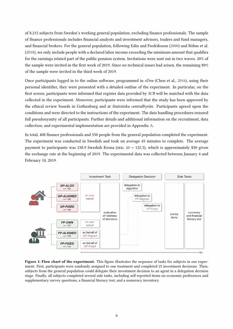
Figure 1: Flow chart of the experiment. This �gure illustrates the sequence of tasks for subjects in our exper-iment. First, participants were randomly assigned to one treatment and completed 25 investment decisions. Then,subjects from the general population could delegate their investment decision to an agent in a delegation decisionstage. Finally, all subjects completed several side tasks, including self-reported items on economic preferences andsupplementary survey questions, a �nancial literacy test, and a numeracy inventory.

6

The sequence of tasks within the experiment is graphically summarized in Figure 1 and described be-low. For detailed information on the main task, please refer to Appendix B. Details on the side tasksand questionnaires are provided in Appendix D. Analyses on subjects’ decision times across subject pools,treatments, and tasks are summarized in Appendix F, outlining high data quality due to moderate varianceacross all sub-samples.

Register data. In addition to the data collected in the online experiment, we obtained register data fromSCB for each participant who completed the experiment. In particular, we received data on demograph-ics (e.g., age, gender, income), occupational history (e.g., workplace, �rm size), subjects’ education, theirwealth history, and military records (e.g., scores of the military suitability tests). See Appendix A for fur-ther details on these variables. In the analysis of experimental results, we only use part of the registrydata as control variables, in particular, participants’ gender (binary indicator for female), age (in years),net income from major employment in 2017 (in thousand ���’s), and maximum education level (dichoto-mous indicators for high school education or less, university education smaller or equal to three years,and university education larger than three years).

Experimental treatments. Depending on the subject pool, participants were randomly assigned to oneof the treatments listed in Table 1. Common to all treatments, both for �nance professionals and for thegeneral population sample, is the 25-item allocation decision task, which is described in detail below.

After having completed all items of the allocation decision task, participants from the general population(principals) had the opportunity to delegate their decisions to an agent. If principals opted for delegatingtheir decisions, the experimental payo� depended on the agent’s rather than their own decisions.4

Depending on the treatment, the principals’ delegationwas either to an investment algorithm programmedby the experimenters (GP-ALGO), a �nance professional with aligned, i.e., linear, incentives (GP-ALIGNED), ora �nance professional receiving a �at payment of 200 ��� for deciding on behalf of one or more clients (GP-FIXED). Note that, compared to the baseline condition GP-FIXED, treatment GP-ALIGNEDmodi�es the incentivestructure of the agent, while holding the type of agent constant. Treatment GP-ALGO modi�es the type ofagent from a human to an investment algorithm.

4 Note that we designed the experiment in a way that each participant made the investment decision �rst, but was informed aboutthe opportunity to delegate the investment decisions only afterwards. Thus, principals do not actually delegate their decisions,but rather decide whether their own or the agent’s decisions are relevant for their payment. While in real-world applications,people usually do not make investment decisions prior to choosing whether or not to delegate, there are practical reasons forthis design choice: First, the opportunity to delegate without prior decisions potentially leads to a high number of delegation inorder to receive an experimental payment without spending any e�ort. Such considerations, however, are not in the focus of thisproject. Second, our design allows examining the allocation decisions of participants who chose to delegate. This way we canstudy whether or not delegation pays o� for those who delegate as well as those who stick to their own decisions. Moreover,we can study risk communication between principals and agents by comparing clients’ and professionals’ investment decisionsconditional on risk levels. However, we cannot account for other potential motives of delegation decisions such as principals’unwillingness to get informed in �nancial matters. Thus, potential “clients” that do not want to engage in �nancial matters at allmight have dropped out initially. For a comprehensive response rate analysis and a discussion of potential self-selection e�ects,please refer to Appendix E.

7

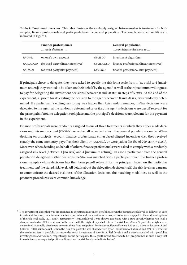
Table 1: Treatment overview. This table illustrates the randomly assigned between-subjects treatments for bothsamples, �nance professionals and participants from the general population. The sample sizes per condition areindicated in Figure 1.

Finance professionals General population. . .make decisions . . . . . . can delegate decisions to . . .

FP-OWN on one’s own account GP-ALGO investment algorithm

FP-ALIGNED for third party (linear incentives) GP-ALIGNED �nance professional (linear incentives)

FP-FIXED for third party (�at payment) GP-FIXED �nance professional (�at payment)

If principals chose to delegate, they were asked to specify the risk (on a scale from 1 [no risk] to 4 [maxi-mum return]) theywanted to be taken on their behalf by the agent,5 as well as their (maximum)willingnessto pay for delegating the investment decisions (between 0 and 50 ���, in steps of 5 ���). At the end of theexperiment, a “price” for delegating the decision to the agent (between 0 and 50 ���) was randomly deter-mined: If a participant’s willingness to pay was higher than this random number, his/her decisions weredelegated to the agent at the randomly determined price (i.e., the agent’s decisions were payo� relevant forthe principal); if not, no delegation took place and the principal’s decisions were relevant for the paymentin the experiment.

Finance professionals were randomly assigned to one of three treatments in which they either made deci-sions on their own account (FP-OWN ), or on behalf of subjects from the general population sample. Whendeciding on principals’ account, �nance professionals either faced aligned incentives (i.e., they receivedexactly the same monetary payo� as their client; FP-ALIGNED), or were paid a �at fee of 200 ��� (FP-FIXED).Moreover, when deciding on behalf of others, �nance professionals were asked to comply with a randomlyassigned risk level (between 1 [no risk] and 4 [maximum return]). In case a participant from the generalpopulation delegated his/her decisions, he/she was matched with a participant from the �nance profes-sional sample (whose decisions has then been payo� relevant for the principal), based on the particulartreatment and the stated risk level. All details about the delegation decision itself, the risk levels as a meansto communicate the desired riskiness of the allocation decisions, the matching modalities, as well as thepayment procedures were common knowledge.

5 The investment algorithm was programmed to construct investment portfolios, given the particular risk level, as follows: In eachinvestment decision, the minimum variance portfolio and the maximum return portfolio were mapped to the endpoint optionsof the risk level scale, i.e., 1 and 4, respectively. Thus, risk level 1 was always associated with a sure payo�, whereas risk level 4always involved a 100% investment in the asset with the highest expected return. For risk levels 2 and 3, portfolio weights weredetermined in equally sized steps between these �xed endpoints. For instance, if payo�s were 2.40 ��� / 0.00 ��� for asset A and0.00 ��� / 0.80 ��� for asset B, then the risk-free portfolio was characterized by an investment of 25% in A and 75% in B, whereasthe maximum return portfolio corresponded to an investment of 100% in A. Risk levels 2 and 3 were associated with portfoliosinvesting 50% and 75% in A, respectively. To the participants the algorithm was described to be “programmed in such a way thatit maximizes your expected pro�t conditional on the risk level you indicate below”.

8

Allocation decision task. The workhorse of our experiment is the allocation decision task as used byBanks et al. (2018). The task consists of 10 decisions with two binary assets in a �rst block, and 15 decisionswith �ve binary assets in a second block. Participants were �rst presented with the task instructions forthe �rst block. After reading the instructions, participants could only continue once they had correctlyanswered three comprehension questions. After the �rst ten decisions, participants were informed that�ve rather than two assets would be available for the remaining 15 decisions. Again, after the instructions,participants had to correctly answer three comprehension questions before proceeding with the task. Theorder of the two blocks was �xed for all subjects, but the order of decisions was randomized in each of thetwo blocks.

For each of the 25 items, participants were informed about the assets’ return per 1 ��� invested dependingon the outcome of a coin toss. The returns for each asset in the 25 investment decisions are depicted inTable B1, and the corresponding opportunity sets are illustrated in Figure B1 in Appendix B. Participantswere endowed with 100 ��� per item and had to allocate the entire endowment on the available assets. Atthe end of the experiment, one of their own or—in case a client opts for delegating the decisions—one ofthe agent’s decisions was randomly chosen, and a simulated coin toss determined the participant’s payo�.Returns were paid on top of the endowment, i.e., payments could not fall below 100 ���.

Decision-making quality measures. The allocation decision task used in this experimental set-up al-lows quantifying decision-making quality based on four di�erent measures. In particular, closely followingBanks et al. (2018), in addition to the expected return (ER) and the standard deviation (SD) of the chosenportfolios we determine a decision-making quality index that comprises the following measures:

• For each decision, we determine violations of the �rst order stochastic dominance principle (FOSD;Hadar and Russell, 1969). In particular, we calculate the di�erence between the expected returnof the chosen portfolio and the highest possible expected return of a portfolio that guarantees thesameminimum payo� as the chosen one. On the participant level, the measures of FOSD are averagedacross all decisions, except for two opportunity sets for which expected returns of all assets wereidentical.

• To quantify violations of the General Axiom of Revealed Preferences (GARP), we utilize the MoneyPump Index (MPI ; Echenique et al., 2011), i.e., the monetary amount a potential arbitrageur couldmake by exploiting a subject’s violations in revealed preferences. On the participant level, we cal-culate the mean money pump cost over all pairwise combinations of opportunity sets.

• Participants’ failure to minimize risk (FMR; Banks et al., 2018) is calculated based on the decisionsin the two opportunity sets for which returns of all allocations were identical, such that the risk-free portfolio (second-order) dominates all other feasible portfolios. A subject’s measure of FMR iscalculated as the mean standard deviation over the two opportunity sets.

• Participants’ �nancial competence (FC; Banks et al., 2018) is measured based on the portfolio choicesin each of four opportunity sets that were identical in the two-assets- and the �ve-assets-frameand/or that were mirrored versions of another opportunity set. A participant’s measure of FC isde�ned as the mean absolute di�erence in expected returns across all identical opportunity sets.

9

For each participant, the predicted values of a principal component analysis of the four measures, FOSD,GARP, FMR, and FC, constitute our decision-making quality index (DMQI). Detailed descriptions on howeach of the decision-making measures is de�ned are provided in Appendix C.

Questionnaires. After the allocation decisions (but prior to the choice whether or not to delegate), allparticipants were asked to self-assess the overall level of risk taken across the 25 items of the allocationdecision task on a scale from 1 to 4, i.e., on the same scale as when choosing the risk level in delegating therisky decisions. In addition, we included the following set of non-incentivized survey items at the end of theexperiment: All participants were asked about (i) their self-assessed risk attitude in general and in �nancialdecisions (Dohmen et al., 2011; Falk et al., 2016), (ii) their willingness to abstain from something today for afuture bene�t (Falk et al., 2016), (iii) their trust in mankind in general, in persons from the �nance industry,and in �nancial algorithms, (iv) their proneness to shift blame on others (Wilson et al., 1990), and (v) theirlevel of prosociality in a hypothetical charitable giving setting (Falk et al., 2018). Furthermore, we includeda 5-item questionnaire on delegation and advice-seeking in �nancial decisions, which was only posed toparticipants that indicate that they have been active in the �nancial market. Afterwards, all participantshad four minutes to answer an 8-item Rasch-validated numeracy inventory (Weller et al., 2013), includingtwo questions on cognitive re�ection. In addition, participants had to provide their self-assessment ofthe number of correct answers in the numeracy questionnaire as well as of their ranking compared toa random sample of the Swedish population. These assessments allow us constructing two measures ofovercon�dence (overestimation and overplacement). Finally, participants had three minutes to answer a6-item �nancial literacy questionnaire based on van Rooij et al., 2011. For further details regarding thesurvey items, please refer to Appendix D.

3. Results

In the following, we �rst answer research question 1 by examining principals’ decisions to delegate acrosstreatments and identifying potential drivers of the choice whether or not to delegate. In a second step, inorder to address research question 2, we examine di�erences in decision-making quality between subjectpools and treatments, serving as a basis for analyzing the e�ectiveness of delegation. Finally, we examinethe communication of risk between principals and agents, providing us with answers to the third researchquestion.

Descriptive results regarding the samples of �nance professionals and the general population, the re-sponses to the questionnaires, and the decision-making quality measures are presented in Tables E1 toTable E4 in Appendix E. Note that detailed descriptions on each of the decision-making measures used inthis section are provided in Appendix C.

Throughout the presentation of the results, we indicate standardized e�ect sizes in terms of marginale�ects at the means (MEM) for non-linear models, and in terms of (absolute) values of Cohen’s d for linearmodels. d is approximated by d ¥ —/(SE·

Ôn), with — denoting the respective regression coe�cient and SE

referring to the corresponding standard error.

10

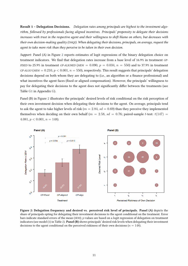
Result 1 – Delegation Decisions. Delegation rates among principals are highest to the investment algo-rithm, followed by professionals facing aligned incentives. Principals’ propensity to delegate their decisionsincreases with trust in the respective agent and their willingness to shift blame on others, but decreases withtheir own decision-making quality (DMQI). When delegating their decisions, principals, on average, request theagent to take more risk than they perceive to be taken in their own decision.

Support: Panel (A) in Figure 2 reports estimates of logit regressions of the binary delegation choice ontreatment indicators. We �nd that delegation rates increase from a base level of 16.9% in treatment GP-FIXED to 25.9% in treatment GP-ALIGNED (MEM = 0.090, p = 0.034, n = 550) and to 37.9% in treatmentGP-ALGO (MEM = 0.210, p < 0.001, n = 550), respectively. This result suggests that principals’ delegationdecisions depend on both whom they are delegating to (i.e., an algorithm or a �nance professional) andwhat incentives the agent faces (�xed or aligned compensation). However, the principals’ willingness topay for delegating their decisions to the agent does not signi�cantly di�er between the treatments (seeTable G1 in Appendix G).

Panel (B) in Figure 2 illustrates the principals’ desired levels of risk conditional on the risk perception oftheir own investment decision when delegating their decisions to the agent. On average, principals tendto ask the agent to take higher levels of risk (m = 2.84, sd = 0.69) than they perceive they implementedthemselves when deciding on their own behalf (m = 2.58, sd = 0.76; paired-sample t-test: t(147) =4.081, p < 0.001, n = 148).

Figure 2: Delegation frequency and desired vs. perceived risk level of principals. Panel (A) depicts theshare of principals opting for delegating their investment decisions to the agent conditional on the treatment. Errorbars indicate standard errors of the mean (SEM); p-values are based on a logit regression of delegation on treatmentindicators (see model (1) in Table 2). Panel (B) shows principals’ desired risk levels when delegating their investmentdecisions to the agent conditional on the perceived riskiness of their own decisions (n = 148).

11

In a second step, we investigate whether behavioral and cognitive measures systematically impact prin-cipals’ decision whether to delegate their decisions to the agent. As indicated by the estimates reportedin model (3) of Table 2, the odds of delegating one’s decision (relative to the delegation rate of 16.9% inthe FP-FIXED condition) are expected to decrease by 22.8% (MEM = 0.045, p = 0.006, n = 550) for a onestandard deviation increase in principals’ decision-making quality index (DMQI). Principals’ trust in theagent turns out to have the largest e�ect on the delegation decision: a one standard deviation increasein (self-reported) trust, on average, implies an increase in the odds of delegating one’s decision to theagent by 98.8% (MEM = 0.115, p < 0.001, n = 550). Similarly, the likelihood for delegating one’s in-vestment decisions tends to increase with a higher propensity for shifting blame to others (MEM = 0.043,p = 0.016, n = 550). Notably, neither numeracy skills and �nancial literacy scores, nor our measures ofovercon�dence, nor participants’ (self-reported) risk tolerance show any explanatory power with respectto principals’ delegation decisions. All results are robust to the inclusion of control variables (see models(2) and (4) in Table 2).6 In addition, we report that none of the drivers of delegation decisions show anysigni�cant impact on participants’ willingness to pay for delegating their choices to the agent (see Table G1in Appendix G).

Result 2 – Decision-Making Quality. Finance professionals deciding on their own account show higherdecision-making quality compared to subjects from the general population only for moderate levels of risktolerance and above. Moreover, professionals’ decision-making quality does not signi�cantly di�er when de-ciding on behalf of clients, neither when being paid a �at fee, nor when facing aligned incentives. On average,delegating the decisions does not pay o� for principals. While �nance professionals do indeed yield slightlyhigher returns than the general population (conditional on the risk level), their portfolios also imply higherportfolio risk.

Support: Given our experimental setup, clients can—assuming that individual-level risk preferences areperfectly mapped by the agents’ decision—only bene�t from delegating their investment decisions, if theagents show superior decision-making quality. Thus, in a �rst step, we compare the decision-making qual-ity index (DMQI) between �nance professionals deciding on their own behalf and the general population. Atwo-sample t-test suggests that �nance professionals are indeed less prone to poor decisions (d = 0.281,t(685) = 2.942, p = 0.003, n = 687; see model (1) in Table G2 in Appendix G). However, by design, errorsin decision-making are less likely, if the decision-maker is risk tolerant.7 Indeed, �nance professionals de-ciding on their own account are signi�cantly less risk averse, in terms of both the mean portfolio risk (SD)taken in the 25 investment decisions (two-sample t-test; d = 0.506, t(685) = 5.302, p < 0.001, n = 687)as well as self-reported risk attitudes in �nancial matters (two-sample t-test; d = 0.818, t(685) = 8.570,p < 0.001, n = 687). Figure 3 shows the linear prediction of decision-making quality based on ordinaryleast squares regressions of DMQI on a subject pool indicator, the portfolio risk (SD), and the interaction of

6 For descriptive results on self-rated trust levels, self-reported risk tolerance, numeracy skills, �nancial literacy, overestimation,and overplacement, please refer to Figures E2–E4 in Appendix G.

7 For instance, consider a risk neutral decision-maker: Choosing an allocation in the task is straightforward as he/she will simplyinvest the entire endowment in the asset yielding the highest expected return. On the other hand, consider a highly risk aversedecision-maker: In order to hedge risks, the decision-maker has to choose well-balanced portfolios. Apparently, the likelihood ofviolating the principle of �rst order stochastic dominance (FOSD) and/or the generalized axiom of revealed preferences (GARP) isconsiderably larger for allocations in the interior of the opportunity sets, compared to boundary allocations.

12

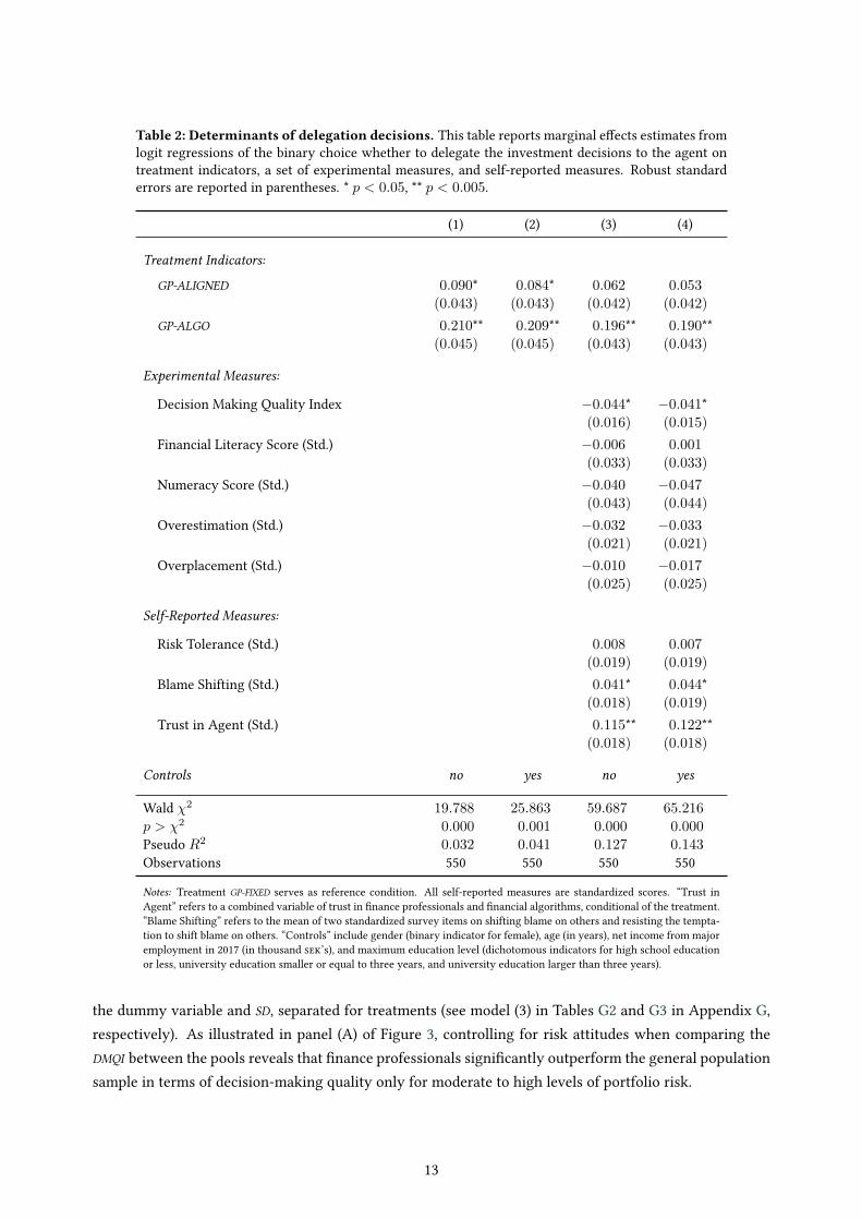
Table 2: Determinants of delegation decisions. This table reports marginal e�ects estimates fromlogit regressions of the binary choice whether to delegate the investment decisions to the agent ontreatment indicators, a set of experimental measures, and self-reported measures. Robust standarderrors are reported in parentheses. * p < 0.05, ** p < 0.005.

(1) (2) (3) (4)

Treatment Indicators:

GP-ALIGNED 0.090* 0.084* 0.062 0.053(0.043) (0.043) (0.042) (0.042)

GP-ALGO 0.210** 0.209** 0.196** 0.190**(0.045) (0.045) (0.043) (0.043)

Experimental Measures:

Decision Making Quality Index ≠0.044* ≠0.041*(0.016) (0.015)

Financial Literacy Score (Std.) ≠0.006 0.001(0.033) (0.033)

Numeracy Score (Std.) ≠0.040 ≠0.047(0.043) (0.044)

Overestimation (Std.) ≠0.032 ≠0.033(0.021) (0.021)

Overplacement (Std.) ≠0.010 ≠0.017(0.025) (0.025)

Self-Reported Measures:

Risk Tolerance (Std.) 0.008 0.007(0.019) (0.019)

Blame Shifting (Std.) 0.041* 0.044*(0.018) (0.019)

Trust in Agent (Std.) 0.115** 0.122**(0.018) (0.018)

Controls no yes no yes

Wald ‰2 19.788 25.863 59.687 65.216

p > ‰2 0.000 0.001 0.000 0.000

Pseudo R2 0.032 0.041 0.127 0.143

Observations 550 550 550 550

Notes: Treatment GP-FIXED serves as reference condition. All self-reported measures are standardized scores. “Trust inAgent” refers to a combined variable of trust in �nance professionals and �nancial algorithms, conditional of the treatment.“Blame Shifting” refers to the mean of two standardized survey items on shifting blame on others and resisting the tempta-tion to shift blame on others. “Controls” include gender (binary indicator for female), age (in years), net income from majoremployment in 2017 (in thousand ���’s), and maximum education level (dichotomous indicators for high school educationor less, university education smaller or equal to three years, and university education larger than three years).

the dummy variable and SD, separated for treatments (see model (3) in Tables G2 and G3 in Appendix G,respectively). As illustrated in panel (A) of Figure 3, controlling for risk attitudes when comparing theDMQI between the pools reveals that �nance professionals signi�cantly outperform the general populationsample in terms of decision-making quality only for moderate to high levels of portfolio risk.

13

In a second step, we examine if �nance professionals’ decision-making quality is systematically impactedby whether they decide on behalf of clients or on their own account, and whether the incentive schemea�ects the proneness to errors in decision-making. A plain comparison of DMQI shows that—compared todeciding for clients and receiving a �at payment (FP-FIXED)—�nance professionals tend to perform betterwhen facing aligned incentives (FP-ALIGNED; d = 0.100, t(405) = 2.019, p = 0.044, n = 408), andwhen deciding on their own account (FP-OWN ; d = 0.132, t(405) = 2.656, p = 0.008, n = 408); seemodel (1) in Table G3 in Appendix G). The di�erence in DMQI between the treatments FP-ALIGNED andFP-OWN is insigni�cant (Wald test; F (1, 405) = 0.426, p = 0.514, n = 408). However, as illustrated inpanels (B) and (C) in Figure 3, the rather small di�erences in decision-making quality between �nanceprofessionals deciding on clients’ behalf and the general population sample turn out being insigni�cantonce we again control for varying levels of portfolio risk (see model (2) in Table G3 in Appendix G fordetails). Finally, panel (D) in Figure 3 depicts the linear predictions of DMQI conditional on mean portfoliorisk for the three treatments FP-OWN , FP-ALIGNED, and FP-FIXED, emphasizing that �nance professionals’decision-making quality is neither systematically a�ected by whether decisions are made on one’s ownbehalf or on clients’ accounts, nor by the compensation scheme the decision-maker faces (see model (3) inTable G3 in Appendix G for details).

As indicated by Result 1, clients take into consideration the agents’ incentive structure when decidingwhether or not to delegate their investment decisions. The latter �nding, however, suggests that clients’expectations regarding the agents’ performance—as re�ected in the di�erence between delegation ratesin treatment GP-FIXED and GP-ALIGNED—are not justi�ed by the performance data, as professionals do notperform systematically better when facing aligned incentives.8

Table 3 summarizes the average decision-making quality (DMQI), expected portfolio returns, and portfoliorisk, separated for �nance professionals deciding on behalf of clients (FP-FIXED and FP-ALIGNED) and thoseprincipals who choose to delegate their decisions, conditional on the risk level principals and agents arematched on, as well as two-sample t-tests for each risk level. As already indicated by Result 2, �nanceprofessionals do not signi�cantly outperform laypeople in terms of decision-making quality for any of thefour risk levels. Comparing the mean expected returns and portfolio risk associated with the allocationdecisions suggests that, conditional on the risk level, �nance professionals tend to generate weakly (andmainly insigni�cantly) higher returns, but at the cost of higher portfolio risk. Thus, overall, principals’delegation decisions to professionals (agents) do not result in more e�cient portfolio allocations in termsof risk-adjusted returns, not even before potential costs of delegation.

Even though delegation has a very modest e�ect on decision quality, it could still be e�ective in terms ofchanging the risk pro�le of the investor. Result 1 reveals that, on average, principals ask the agents to

8 In Appendix F, we report detailed analyses on decision times across subject pools, treatments, and tasks. We observe, for instance,that professionals take more time when deciding for clients compared to when deciding on their on behalf, and compared toclients’ own decisions in the two-asset opportunity sets (see Table F2 for details). However, in the �ve-asset cases, di�erences intime spent between clients and professionals vanish, suggesting that clients took the more complex tasks seriously. Together withResult 2, these �ndings might indicate that professionals really strive for meeting clients’ expectations (i.e., desired risk levels),even though it does not translate into better performance in our sample. Furthermore, we examine potential learning e�ects inthe investment task and the impact of the time spent per investment decision on decision-making quality. While we identify asigni�cant decrease in the average time spent per investment decision for subsequent decisions in both subject pools, we reportthat the time spent per decision does not signi�cantly impact decision-making quality, neither among the general population,nor the �nance professionals sample; please refer to Appendix F for details.

14

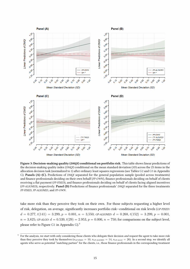
Figure 3: Decision-making quality (DMQI) conditional on portfolio risk. This table shows linear predictions ofthe decision-making quality index (DMQI ) conditional on the mean standard deviation (SD) across the 25 items in theallocation decision task (normalized to 1) after ordinary least squares regressions (see Tables G2 and G3 in AppendixG). Panels (A)–(C). Predictions of DMQI separated for the general population sample (pooled across treatments)and �nance professionals deciding on their own behalf (FP-OWN ), �nance professionals deciding on behalf of clientsreceiving a �at payment (FP-FIXED), and �nance professionals deciding on behalf of clients facing aligned incentives(FP-ALIGNED), respectively. Panel (D) Predictions of �nance professionals’ DMQI separated for the three treatmentsFP-FIXED, FP-ALIGNED, and FP-OWN .

take more risk than they perceive they took on their own. For those subjects requesting a higher levelof risk, delegation, on average, signi�cantly increases portfolio risk—conditional on risk levels (GP-FIXED:d = 0.277, t(141) = 3.299, p = 0.001, n = 3,550; GP-ALIGNED: d = 0.268, t(152) = 3.299, p = 0.001,n = 3,825; GP-ALGO: d = 0.539, t(29) = 2.953, p = 0.006, n = 750; for comparisons on the subject level,please refer to Figure G1 in Appendix G).9

9 For the analysis, we start with only considering those clients who delegate their decision and request the agent to take more riskthan they perceive they took by themselves (nGP-FIXED = 10, nGP-ALIGNED = 14, nGP-ALGO = 26). In a second step, we identify allagents who serve as potential “matching partner” for the clients, i.e., those �nance professionals in the corresponding treatment

15

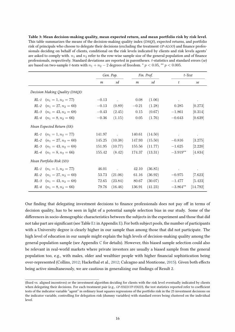
Table 3: Mean decision-making quality, mean expected return, and mean portfolio risk by risk level.This table summarizes the means of the decision-making quality index (DMQI ), expected returns, and portfoliorisk of principals who choose to delegate their decisions (excluding the treatment GP-ALGO) and �nance profes-sionals deciding on behalf of clients, conditional on the risk levels indicated by clients and risk levels agents’are asked to comply with. n1 and n2 refer to the row-wise sample size of the general population and of �nanceprofessionals, respectively. Standard deviations are reported in parentheses. t-statistics and standard errors (se)are based on two-sample t-tests with n1 + n2 ≠ 2 degrees of freedom. * p < 0.05, ** p < 0.005.

Gen. Pop. Fin. Prof. t-Test

m sd m sd t se

Decision Making Quality (DMQI):

RL-1 (n1 = 1, n2 = 77) ≠0.13 . 0.08 (1.06) . .RL-2 (n1 = 27, n2 = 60) ≠0.13 (0.89) ≠0.21 (1.28) 0.285 [0.273]RL-3 (n1 = 43, n2 = 68) ≠0.43 (2.45) 0.15 (0.67) ≠1.861 [0.314]RL-4 (n1 = 8, n2 = 66) ≠0.36 (1.15) 0.05 (1.76) ≠0.643 [0.639]

Mean Expected Return (ER):

RL-1 (n1 = 1, n2 = 77) 141.97 . 140.61 (14.50) . .RL-2 (n1 = 27, n2 = 60) 145.25 (10.38) 147.93 (15.50) ≠0.816 [3.275]RL-3 (n1 = 43, n2 = 68) 151.95 (10.77) 155.56 (11.77) ≠1.625 [2.220]RL-4 (n1 = 8, n2 = 66) 155.42 (8.42) 174.37 (13.31) ≠3.919** [4.834]

Mean Portfolio Risk (SD):

RL-1 (n1 = 1, n2 = 77) 46.01 . 42.10 (36.85) . .RL-2 (n1 = 27, n2 = 60) 53.73 (21.06) 61.16 (36.92) ≠0.975 [7.623]RL-3 (n1 = 43, n2 = 68) 72.65 (23.84) 80.67 (30.07) ≠1.477 [5.423]RL-4 (n1 = 8, n2 = 66) 79.76 (16.46) 136.91 (41.23) ≠3.864** [14.792]

Our �nding that delegating investment decisions to �nance professionals does not pay o� in terms ofdecision quality, has to be seen in light of a potential sample selection bias in our study. Some of thedi�erences in socio-demographic characteristics between the subjects in the experiment and those that didnot take part are signi�cant (see Table E1 in Appendix E). For both subject pools, the number of participantswith a University degree is clearly higher in our sample than among those that did not participate. Thehigh level of education in our sample might explain the high levels of decision-making quality among thegeneral population sample (see Appendix C for details). However, this biased sample selection could alsobe relevant in real-world markets where private investors are usually a biased sample from the generalpopulation too, e.g., with males, older and wealthier people with higher �nancial sophistication beingover-represented (Collins, 2012; Hackethal et al., 2012; Calcagno and Monticone, 2015). Given both e�ectsbeing active simultaneously, we are cautious in generalizing our �ndings of Result 2.

(�xed vs. aligned incentives) or the investment algorithm deciding for clients with the risk level eventually indicated by clientswhen delegating their decisions. For each treatment pair (e.g., GP-FIXED/FP-FIXED), the test statistics reported refer to coe�cienttests of the indicator variable “agent” in ordinary least squares regressions of the portfolio risk in the 25 investment decisions onthe indicator variable, controlling for delegation risk (dummy variables) with standard errors being clustered on the individuallevel.

16

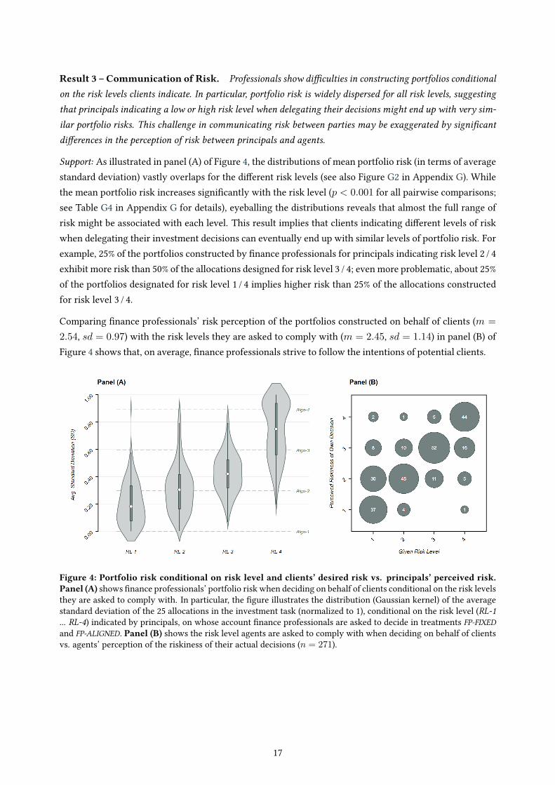
Result 3 – Communication of Risk. Professionals show di�culties in constructing portfolios conditionalon the risk levels clients indicate. In particular, portfolio risk is widely dispersed for all risk levels, suggestingthat principals indicating a low or high risk level when delegating their decisions might end up with very sim-ilar portfolio risks. This challenge in communicating risk between parties may be exaggerated by signi�cantdi�erences in the perception of risk between principals and agents.

Support: As illustrated in panel (A) of Figure 4, the distributions of mean portfolio risk (in terms of averagestandard deviation) vastly overlaps for the di�erent risk levels (see also Figure G2 in Appendix G). Whilethe mean portfolio risk increases signi�cantly with the risk level (p < 0.001 for all pairwise comparisons;see Table G4 in Appendix G for details), eyeballing the distributions reveals that almost the full range ofrisk might be associated with each level. This result implies that clients indicating di�erent levels of riskwhen delegating their investment decisions can eventually end up with similar levels of portfolio risk. Forexample, 25% of the portfolios constructed by �nance professionals for principals indicating risk level 2 / 4exhibit more risk than 50% of the allocations designed for risk level 3 / 4; even more problematic, about 25%of the portfolios designated for risk level 1 / 4 implies higher risk than 25% of the allocations constructedfor risk level 3 / 4.

Comparing �nance professionals’ risk perception of the portfolios constructed on behalf of clients (m =2.54, sd = 0.97) with the risk levels they are asked to comply with (m = 2.45, sd = 1.14) in panel (B) ofFigure 4 shows that, on average, �nance professionals strive to follow the intentions of potential clients.

Figure 4: Portfolio risk conditional on risk level and clients’ desired risk vs. principals’ perceived risk.Panel (A) shows �nance professionals’ portfolio risk when deciding on behalf of clients conditional on the risk levelsthey are asked to comply with. In particular, the �gure illustrates the distribution (Gaussian kernel) of the averagestandard deviation of the 25 allocations in the investment task (normalized to 1), conditional on the risk level (RL-1... RL-4) indicated by principals, on whose account �nance professionals are asked to decide in treatments FP-FIXEDand FP-ALIGNED. Panel (B) shows the risk level agents are asked to comply with when deciding on behalf of clientsvs. agents’ perception of the riskiness of their actual decisions (n = 271).

17

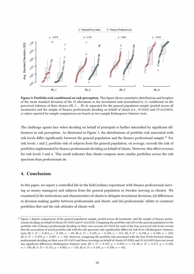
Figure 5: Portfolio risk conditional on risk perception. This �gure shows cumulative distributions and boxplotsof the mean standard deviation of the 25 allocations in the investment task (normalized to 1), conditional on theperceived riskiness of their choices (RL-1 ... RL-4), separated for the general population sample (pooled across alltreatments) and the sample of �nance professionals deciding on behalf of clients (i.e., FP-FIXED and FP-ALIGNED).p-values reported for sample comparisons are based on two-sample Kolmogorov-Smirnov tests.

The challenge agents face when deciding on behalf of principals is further intensi�ed by signi�cant dif-ferences in risk perception. As illustrated in Figure 5, the distributions of portfolio risk associated withrisk levels di�er signi�cantly between the general population and the �nance professional sample.10 Forrisk levels 1 and 2, portfolio risk of subjects from the general population, on average, exceeds the risk ofportfolios implemented by �nance professionals deciding on behalf of clients. However, this e�ect reversesfor risk levels 3 and 4. This result indicates that clients compose more similar portfolios across the riskspectrum than professionals do.

4. Conclusion

In this paper, we report a controlled lab-in-the �eld (online) experiment with �nance professionals (serv-ing as money managers) and subjects from the general population in Sweden (serving as clients). Weexamined (i) the motivations and characteristics of clients to delegate investment decisions, (ii) di�erencesin decision-making quality between professionals and clients, and (iii) professionals’ ability to constructportfolios that suit the risk attitudes of clients well.

10 Figure 5 depicts comparisons of the general population sample, pooled across all treatments, and the sample of �nance profes-sionals deciding on behalf of clients (FP-FIXED and FP-ALIGNED). Comparing the portfolio risk (SD) of the general population to theportfolio risk of �nance professionals deciding on their own account (FP-OWN ) for each of the four perceived risk levels revealsthat the association of actual portfolio risk with the risk spectrum only signi�cantly di�ers for risk level 4 (Kolmogorov-Smirnovtests; RL-1: D = 0.354, p = 0.180, n = 60; RL-2: D = 0.195, p = 0.108, n = 311; RL-3: D = 0.198, p = 0.100, n = 232;RL-4: D = 0.379, p = 0.007, n = 84). However, comparing the portfolio risk associated with the four levels between �nanceprofessionals deciding on their own (FP-OWN ) and those investing on behalf of clients (FP-FIXED and FP-ALIGNED) does not revealany signi�cant di�erences (Kolmogorov-Smirnov tests; RL-1: D = 0.167, p = 0.958, n = 54; RL-2: D = 0.157, p = 0.450,n = 136; RL-3: D = 0.131, p = 0.663, n = 134; RL-4: D = 0.185, p = 0.506, n = 84).

18

First, we found that investors delegated to the investment algorithm signi�cantly more often than to pro-fessionals with aligned incentives and �at incentives. Furthermore, we reported that those investors withthe highest levels of trust in professionals (investment algorithms) and those who are prone to shift blameon others delegated the most, whereas we found that principals’ own decision-making quality was neg-atively related to the delegation frequency. Second, we found that overall decision-making quality ofprofessionals was not signi�cantly better than that of subjects from the general population. Finally, weobserved that professionals had di�culties in constructing portfolios conditional on the risk-levels clientsindicated. In particular, we found strong overlaps in portfolio risks especially among three of the four riskclasses.

Our study has implications for real-world delegation decisions: �rst, clients with low decision-makingquality and/or high level of trust in professionals/algorithms are indeed the ones that delegate more fre-quently. This result highlights the importance of establishing trust in the �nance industry in general andin money managers in particular, as it appears to be one of the major motives for delegation decisions.However, professionals’ decision-making quality is only marginally and not signi�cantly better than thatof clients. We still conclude that for the clients that trust professionals or �nancial algorithms, delegationis probably a good choice, as they “purchase” slightly better decisions and are con�dent that professionalsdo it well. In other words, “money doctors” (Gennaioli et al., 2015) are trusted when investing money oftheir clients, even when the outcome is not signi�cantly better.

Second, our results indicate that some clients use delegation as way of increasing the risk of their portfolio,but the feasibility of this objective is hampered by our �nding that professionals face troubles in correctlyimplementing clients’ expected portfolio risk-level. The issue of risk communication is particularly rele-vant for real-world delegation of �nancial decisions and related to the empirical studies of Foerster et al.(2017) and Linnainmaa et al. (2019). Both studies show that �nancial advisers typically invest personallyjust as they advise their clients. Thus, we conclude that a better match of advisers and clients in termsof risk preferences and potentially also with respect to risk perception (Holzmeister et al., 2019) might bebene�cial both for clients and �nancial institutions.

19

References

Abdellaoui, M., Baillon, A., Placido, L., & Wakker, P. P. (2011). The rich domain of uncertainty: Sourcefunctions and their experimental implementation. American Economic Review, 101(2), 695–723.

Abdellaoui, M., Bleichrodt, H., & Kammoun, H. (2013). Do �nancial professionals behave according toprospect theory? An experimental study. Theory and Decision, 74(3), 411–429.

Alevy, J. E., Haigh, M. S., & List, J. A. (2007). Information cascades: Evidence from a �eld experiment with�nancial market professionals. Journal of Finance, 62(1), 151–180.

Andersson, O., Holm, H. J., Tyran, J.-R., & Wengström, E. (2016). Deciding for others reduces loss aversion.Management Science, 62(1), 29–36.

Andersson, O., Holm, H. J., Tyran, J.-R., & Wengström, E. (2019). Risking other people’s money: Experi-mental evidence on bonus schemes, competition, and altruism. Scandinavian Journal of Economics,online �rst, 1–27.

Banks, J., Carvalho, L., & Perez-Arce, F. (2018). Education, decision-making, and economic rationality.Review of Economics and Statistics, 101(3), 428–441.

Bartling, B., & Fischbacher, U. (2012). Shifting the blame: On delegation and responsibility. Review of Eco-nomic Studies, 79(1), 67–87.

Bebchuk, L., & Spamann, H. (2010). Regulating bankers’ pay. Georgetown Law Journal, 98(2), 247–287.

Böhm, M., Metzger, D., & Strömberg, P. (2018). Since you are so rich, you must be really smart: Talent andthe �nance wage premium. Riksbank Research Paper Series No. 137.

Bolton, G., & Ockenfels, A. (2010). Betrayal aversion: Evidence from Brazil, China, Oman, Switzerland,Turkey, and the United States: Comment. American Economic Review, 100(1), 628–633.

Calcagno, R., & Monticone, C. (2015). Financial literacy and the demand for �nancial advice. Journal ofBanking and Finance, 50, 363–380.

Carhart, M. M. (1997). On Persistence in Mutual Fund Performance. Journal of Finance, 52(1), 57–82.

Chakravarty, S., Harrison, G., Haruvy, E., & Rutström, E. (2011). Are you risk averse over other peoples’money? Southern Economic Journal, 77 (4), 901–913.

Chang, T., Solomon, D., & Wester�eld, M. (2016). Looking for someone to blame: Delegation, cognitivedissonance, and the disposition e�ect. The Journal of Finance, 71(1), 267–302.

Chen, D. L., Schonger, M., & Wickens, C. (2016). oTree—An open-source platform for laboratory, online,and �eld experiments. Journal of Behavioral and Experimental Finance, 9, 88–97.

Cipriani,M., &Guarino, A. (2009). Herd behavior in�nancialmarkets: An experimentwith�nancialmarketprofessionals. Journal of the European Economic Association, 7 (1), 206–233.

Collins, J. M. (2012). Financial advice: A substitute for �nancial literacy? Financial Services Review, 21(4),307–322.

D’Acunto, F., Prabhala, N., & Rossi, A. (2019). The promises and pitfalls of robo-advising. The Review ofFinancial Studies, 32(5), 1983–2020.

Dewatripont, M., & Freixas, X. (2012). Bank resolution: Lessons from the crisis. In M. Dewatripont & X.Freixas (Eds.), The crisis aftermath: New regulatory paradigms. London: Centre for Economic PolicyResearch.

20

Diamond, D. W., & Rajan, R. G. (2009). The credit crisis: Conjectures about causes and remedies. AmericanEconomic Review, 99(2), 606–610.

Dietvorst, B., Simmons, J., & Massey, C. (2014). Algorithm aversion: People erroneously avoid algorithmsafter seeing them err. Journal of Experimental Psychology: General, 144(1), 114–126.

Dohmen, T., Falk, A., Hu�man, D., Sunde, U., Schupp, J., &Wagner, G. (2011). Individual risk attitudes: Mea-surement, determinants and behavioral consequences. Journal of the European Economic Association,9(3), 522–550.

Dulleck, U., & Kerschbamer, R. (2006). On doctors, mechanics, and computer specialists: The economics ofcredence goods. Journal of Economic Literature, 44(1), 5–42.

Echenique, F., Lee, S., & Shum, M. (2011). The Money Pump as a measure of revealed preference violations.Journal of Political Economy, 119(6), 1201–1223.

Edin, P., & Fredriksson, P. (2000). LINDA: Longitudinell individual data for Sweden.Working Paper.

Eriksen, K., & Kvaløy, O. (2010). Myopic investment management. Review of Finance, 14(3), 521–542.

Eriksen, K., Kvaløy, O., & Luzuriaga, M. (2017). Risk-taking on behalf of others. CESifo Working Paper SeriesNo. 6378.

Falk, A., Becker, A., Dohmen, T., Enke, B., Hu�man, D., & Sunde, U. (2018). Global evidence on economicpreferences. Quarterly Journal of Economics, 133(4), 1645–1692.

Falk, A., Becker, A., Dohmen, T., Hu�man, D., & Sunde, U. (2016). The Preference Survey Module: A val-idated instrument for measuring risk, time, and social preferences. IZA Discussion Paper Series No.9674.

Financial Crisis Inquiry Commission. (2011). The Financial Crisis Inquiry Report: Final report of the NationalCommission on the causes of the �nancial and economic crisis in the United States. Washington, DC:U.S. Government Printing O�ce.

Foerster, S., Linnaimaa, J. T., Melzer, B. T., & Previtero, A. (2017). Retail �nancial advice: Does one size �tall? Journal of Finance, 72(4), 1441–1482.

Frederick, S. (2005). Cognitive re�ection and decision making. Journal of Economic Perspectives, 19(4), 25–42.

French, K. R. (2008). Presidential Address: The cost of active investing. The Journal of Finance, 63(4), 1537–1573.

Füllbrunn, S., & Luhan,W. (2015). Am Imy peer’s keeper? Social responsibility in �nancial decisionmaking.Ruhr Economic Papers #551.

Gennaioli, N., Shleifer, A., & Vishny, R. (2015). Money doctors. Journal of Finance, 70(1), 91–114.

Gruber, M. J. (1996). Another puzzle: The growth in actively managed mutual funds. The Journal of Finance,51(3), 783–810.

Guiso, L., Sapienza, P., & Zingales, L. (2004). The role of social capital in �nancial development. AmericanEconomic Review, 94(3), 526–556.

Guiso, L., Sapienza, P., & Zingales, L. (2008). Trusting the stock market. The Journal of Finance, 63(6), 2557–2600.

21

Hackethal, A., Haliassos, M., & Jappelli, T. (2012). Financial advisors: A case of babysitters? Journal ofBanking and Finance, 36(2), 509–524.

Hadar, J., & Russell, W. (1969). Rules for ordering uncertain prospects. American Economic Review, 59(1),25–34.

Haigh, M. S., & List, J. A. (2005). Do professional traders exhibit myopic loss aversion? An experimentalanalysis. Journal of Finance, 60(1), 523–534.

Harvey, C., Rattray, S., Sinclair, A., & Van Hemert, O. (2017). Man vs. machine: Comparing discretionaryand systematic hedge fund performance. Journal of Portfolio Management, 43(4), 55–69.

Holt, C. A., & Laury, S. K. (2002). Risk Aversion and Incentive E�ects. American Economic Review, 92(5),1644–1655.

Holzmeister, F., Huber, J., Kirchler, M., Lindner, F., Weitzel, U., & Zeisberger, S. (2019). What drives riskperception? A global survey with �nancial professionals and lay people.Management Science, forth-coming.

Ifcher, J., & Zarghamee, H. (2019). Behavioral economic phenomena in decision-making for others. Journalof Economic Psychology, forthcoming.

Inderst, R., & Ottaviani, M. (2012a). Competition through commissions and kickbacks. American EconomicReview, 102(2), 780–809.

Inderst, R., & Ottaviani, M. (2012b). Financial advice. Journal of Economic Literature, 50(2), 494–512.

Inderst, R., & Ottaviani, M. (2012c). How (not) to pay for advice: A framework for consumer �nancialprotection. Journal of Financial Economics, 105(2), 393–411.

Jensen, M. C. (1968). The performance of mutual funds in the period 1945–1964. The Journal of Finance,23(2), 389–416.

Jensen, M. C., & Meckling, W. H. (1976). Theory of the �rm: Managerial behavior, agency costs, and own-ership structure. Journal of Financial Economics, 3(4), 305–360.

Kaustia, M., Alho, E., & Puttonen, V. (2008). How much does expertise reduce behavioral biases? The caseof anchoring e�ects in stock return estimates. Financial Management, 37 (3), 391–412.

Kirchler, M., Lindner, F., & Weitzel, U. (2018a). Delegated decision making and social competition in the�nance industry.Working Papers in Economics and Statistics, University of Innsbruck.

Kirchler, M., Lindner, F., & Weitzel, U. (2018b). Rankings and risk-taking in the �nance industry. Journalof Finance, 73(5), 2271–2302.

Kling, L., König-Kersting, C., & Trautmann, S. T. (2019). Investment preferences and risk perception: Fi-nancial agents versus clients. AWI Discussion Paper Series No. 674.

Lachance, M.-E., & Tang, N. (2012). Financial advice and trust. Financial Services Review, 21(3), 209–226.

Linnainmaa, J. T., Melzer, B., & Previtero, A. (2019). The misguided beliefs of �nancial advisors. The Journalof Finance, forthcoming.

Logg, J., Minson, J., & Moore, D. (2017). Algorithm appreciation: People prefer algorithmic to human judg-ment. Organizational Behavior and Human Decision Processes, 151, 90–103.

Longoni, C., Bonezzi, A., & Morewedge, C. K. (2019). Resistance to medical arti�cial intelligence. Journalof Consumer Research, 46(4), 629–650.

22

Mullainathan, S., Noeth, M., & Schoar, A. (2012). The market for �nancial advice: An audit study. NBERWorking Paper No. 17929.

Rajan, R. G. (2006). Has �nance made the world riskier? European Financial Management, 12(4), 499–533.

Rud, O. A., Rabanal, J. P., & Horowitz, J. (2018). Does competition aggravate moral hazard? A multi-principal-agent experiment. Journal of Financial Intermediation, 33, 115–121.

Schwaiger, R., Kirchler, M., Lindner, F., & Weitzel, U. (2019). Determinants of investor expectations andsatisfaction: A study with �nancial professionals. Journal of Economic Dynamics and Control, forth-coming.

Shefrin, H. (2007). Beyond greed and fear: Understanding behavioral �nance and the psychology of investing.Oxford: Oxford University Press.

Sutter, M. (2009). Individual behavior and group membership: Comment. American Economic Review, 99(5),2247–2257.

Toplak, M. E., West, R. F., & Stanovich, K. E. (2014). Assessing miserly information processing: An expan-sion of the Cognitive Re�ection Test. Thinking and Reasoning, 20(2), 147–168.

van Rooij, M., Lusardi, A., & Alessie, R. (2011). Financial literacy and stock market participation. Journalof Financial Economics, 101(2), 449–472.

Vieider, F. M., Villegas-Palacio, C., Martinsson, P., & Mejía, M. (2016). Risk taking for oneself and others:A structural model approach. Economic Inquiry, 54(2), 879–894.

Weitzel, U., Huber, C., Huber, J., Kirchler, M., Lindner, F., & Rose, J. (2019). Bubbles and �nancial profes-sionals. Review of Financial Studies, forthcoming.

Weller, J. A., Dieckmann, N. F., Tusler, M., Mertz, C. K., Burns, W. J., & Peters, E. (2013). Development andtesting of an abbreviated numeracy scale: A Rasch analysis approach. Journal of Behavioral DecisionMaking, 26(2), 198–212.

Wilson, G., Gray, J., & Barrett, P. (1990). A factor analysis of the Gray-Wilson personality questionnaire.Personality and Individual Di�erences, 11(10), 1037–1044.

23

Appendices

Delegated Decision-Making in Finance

Felix Holzmeister† Martin Holmén‡,ú Michael Kirchler†,‡

Matthias Stefan† Erik Wengström§,¶

† University of Innsbruck, Department of Banking and Finance‡ University of Gothenburg, Department of Economics, Centre for Finance

§ Lund University, Department of Economics¶ Hanken School of Economics, Department of Finance and Economics

ú Corresponding author: martin.holmen@gu.se

Contents

A Data collection and Recruitment . . . . . . . . . . . . . . . . . . . . . . . . . . . . . . . . . . 1B Allocation Decision Task . . . . . . . . . . . . . . . . . . . . . . . . . . . . . . . . . . . . . . 3C Decision-Making Quality Measures . . . . . . . . . . . . . . . . . . . . . . . . . . . . . . . . 5D Questionnaires and Side Tasks . . . . . . . . . . . . . . . . . . . . . . . . . . . . . . . . . . . 10E Descriptive Results. . . . . . . . . . . . . . . . . . . . . . . . . . . . . . . . . . . . . . . . . . 15F Descriptives and Analyses of Time Spent . . . . . . . . . . . . . . . . . . . . . . . . . . . . . 25G Supplementary Results . . . . . . . . . . . . . . . . . . . . . . . . . . . . . . . . . . . . . . . 27

List of Tables

B1. Parameters of the 25 opportunity sets. . . . . . . . . . . . . . . . . . . . . . . . . . . . . . . 3C1. Principal component analysis of the four decision-making quality measures. . . . . . . . . 9D1. Survey questions. . . . . . . . . . . . . . . . . . . . . . . . . . . . . . . . . . . . . . . . . . 12D2. Numeracy inventory based on Weller et al. (2013). . . . . . . . . . . . . . . . . . . . . . . . 13D3. Financial literacy inventory based on van Rooij et al. (2011). . . . . . . . . . . . . . . . . . 14E1. Sample characteristics by subject pools. . . . . . . . . . . . . . . . . . . . . . . . . . . . . . 17E2. Descriptive statistics of the decision-making quality measures. . . . . . . . . . . . . . . . . 18E3. Di�erences in decision-making quality measures. . . . . . . . . . . . . . . . . . . . . . . . 18E4. Correlations between the decision-making quality measures. . . . . . . . . . . . . . . . . . 19E5. Descriptive statistics and comparisons between pools for the survey items. . . . . . . . . . 20E6. Descriptive statistics for numeracy, �nancial literacy, and overcon�dence. . . . . . . . . . 21F1. Descriptive statistics of time spent per task. . . . . . . . . . . . . . . . . . . . . . . . . . . . 26F2. Di�erences in time spent. . . . . . . . . . . . . . . . . . . . . . . . . . . . . . . . . . . . . . 26G1. Willingness to pay for delegation. . . . . . . . . . . . . . . . . . . . . . . . . . . . . . . . . 27G2. Decision-making quality by subject pool. . . . . . . . . . . . . . . . . . . . . . . . . . . . . 28G3. Finance professionals’ decision-making quality by treatments. . . . . . . . . . . . . . . . . 29G4. Finance professionals’ risk taking when deciding on behalf of clients. . . . . . . . . . . . . 30

List of Figures

B1. Opportunity sets in the allocation decision task. . . . . . . . . . . . . . . . . . . . . . . . . 4C1. Violation of the principle of �rst order stochastic dominance (FOSD). . . . . . . . . . . . . . 6C2. Violation of the generalized axiom of revealed preferences. . . . . . . . . . . . . . . . . . . 7E1. Self-reported risk tolerance. . . . . . . . . . . . . . . . . . . . . . . . . . . . . . . . . . . . 22E2. Self-reported trust. . . . . . . . . . . . . . . . . . . . . . . . . . . . . . . . . . . . . . . . . 23E3. Numeracy and �nancial literacy scores. . . . . . . . . . . . . . . . . . . . . . . . . . . . . . 24E4. Overestimation and overplacement. . . . . . . . . . . . . . . . . . . . . . . . . . . . . . . . 24G1. Portfolio risk of clients’ asking the agent to take more risk when delegating. . . . . . . . . 31G2. Number of portfolios with similar portfolio risk across risk levels. . . . . . . . . . . . . . . 32

A. Data collection and Recruitment

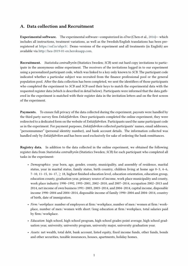
Experimental software. The experimental software—computerized in oTree (Chen et al., 2016)— whichincludes all instructions, treatment variations, as well as the Swedish/English translations has been pre-registered at https://osf.io/ubpr3/. Demo versions of the experiment and all treatments (in English) areavailable via http://hea-2019-01-en.herokuapp.com.

Recruitment. Statistiska centralbyro̊n (Statistics Sweden; SCB) sent out hard copy invitations to partic-ipate in the anonymous online experiment. The receivers of the invitations logged in to our experimentusing a personalized participant code, which was linked to a key only known to SCB. The participant codeindicated whether a particular subject was recruited from the �nance professional pool or the generalpopulation pool. After the data collection has been completed, we sent the identi�ers of those participantswho completed the experiment to SCB and SCB used their keys to match the experimental data with therequested register data (which is described in detail below). Participants were informed that the data gath-ered in the experiment is matched with their register data in the invitation letters and on the �rst screenof the experiment.

Payments. To ensure full privacy of the data collected during the experiment, payouts were handled bythe third party survey �rm Enkätfabriken. Once participants completed the online experiment, they wereredirected to a dedicated form on the website of Enkätfabriken. Participants used the same participant codeas in the experiment. For payment purposes, Enkätfabriken collected participants’ names, email addresses,“personnummer” (personal identity number), and bank account details. The information collected washandled only by Enkätfabriken and has been used exclusively for sake of ordering the bank remittances.

Registry data. In addition to the data collected in the online experiment, we obtained the followingregister data from Statistiska centralbyro̊n (Statistics Sweden; SCB) for each participant who completed alltasks in the experiment:

• Demographics: year born, age, gender, county, municipality, and assembly of residence, maritalstatus, year in marital status, family status, birth country, children living at home age 0–3, 4–6,7–10, 11–15, 16–17, Ø 18, highest �nished education level, education orientation, education group,education county, graduation year, primary source of income, work place municipality and county,work place industry 1990–1992, 1993–2001, 2002–2010, and 2007–2014, occupation 2002–2013 and2014, net income of own business 1991–2003, 2003–2014, and 2004–2014, capital income, disposableincome 1990–2004 and 2004–2014, disposable income of family 1990–2004 and 2004–2014, countryof birth, date of immigration.

• Firm /workplace: number of employees at �rm /workplace, number of men /women at �rm /work-place, number of men /women with short / long education at �rm /workplace, total salaries paidby �rm /workplace.

• Education: high school, high school program, high school grades point average, high school grad-uation year, university, university program, university major, university graduation year.

• Assets: net wealth, total debt, bank account, listed equity, �xed income funds, other funds, bondsand other securities, taxable insurances, houses, apartments, holiday homes.

1

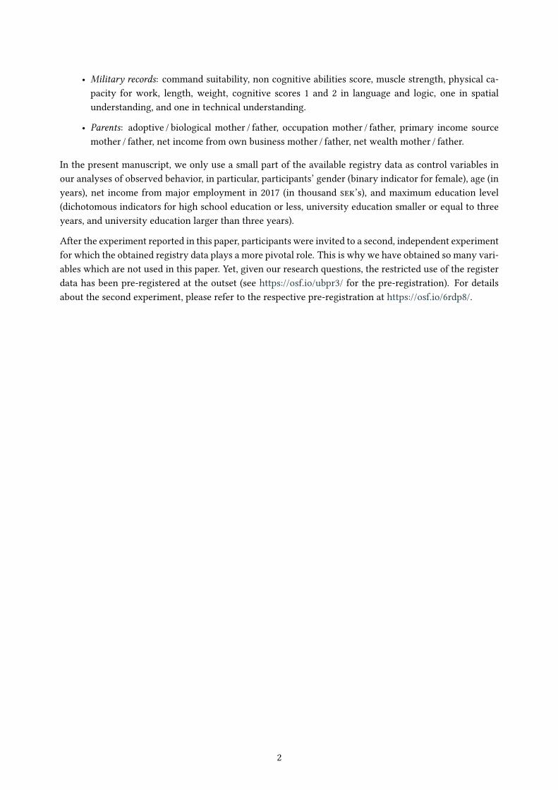
• Military records: command suitability, non cognitive abilities score, muscle strength, physical ca-pacity for work, length, weight, cognitive scores 1 and 2 in language and logic, one in spatialunderstanding, and one in technical understanding.

• Parents: adoptive / biological mother / father, occupation mother / father, primary income sourcemother / father, net income from own business mother / father, net wealth mother / father.

In the present manuscript, we only use a small part of the available registry data as control variables inour analyses of observed behavior, in particular, participants’ gender (binary indicator for female), age (inyears), net income from major employment in 2017 (in thousand ���’s), and maximum education level(dichotomous indicators for high school education or less, university education smaller or equal to threeyears, and university education larger than three years).

After the experiment reported in this paper, participants were invited to a second, independent experimentfor which the obtained registry data plays a more pivotal role. This is why we have obtained so many vari-ables which are not used in this paper. Yet, given our research questions, the restricted use of the registerdata has been pre-registered at the outset (see https://osf.io/ubpr3/ for the pre-registration). For detailsabout the second experiment, please refer to the respective pre-registration at https://osf.io/6rdp8/.

2

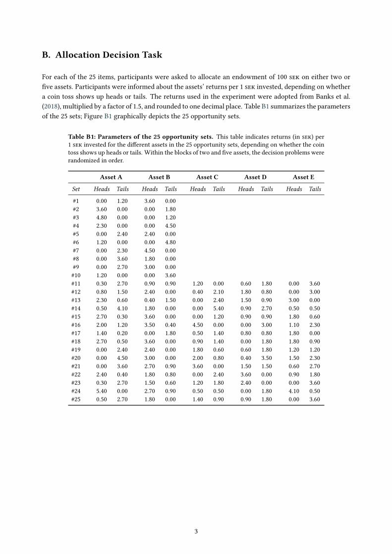
B. Allocation Decision Task

For each of the 25 items, participants were asked to allocate an endowment of 100 ��� on either two or�ve assets. Participants were informed about the assets’ returns per 1 ��� invested, depending on whethera coin toss shows up heads or tails. The returns used in the experiment were adopted from Banks et al.(2018), multiplied by a factor of 1.5, and rounded to one decimal place. Table B1 summarizes the parametersof the 25 sets; Figure B1 graphically depicts the 25 opportunity sets.

Table B1: Parameters of the 25 opportunity sets. This table indicates returns (in ���) per1 ��� invested for the di�erent assets in the 25 opportunity sets, depending on whether the cointoss shows up heads or tails. Within the blocks of two and �ve assets, the decision problems wererandomized in order.

Asset A Asset B Asset C Asset D Asset E

Set Heads Tails Heads Tails Heads Tails Heads Tails Heads Tails

#1 0.00 1.20 3.60 0.00#2 3.60 0.00 0.00 1.80#3 4.80 0.00 0.00 1.20#4 2.30 0.00 0.00 4.50#5 0.00 2.40 2.40 0.00#6 1.20 0.00 0.00 4.80#7 0.00 2.30 4.50 0.00#8 0.00 3.60 1.80 0.00#9 0.00 2.70 3.00 0.00#10 1.20 0.00 0.00 3.60#11 0.30 2.70 0.90 0.90 1.20 0.00 0.60 1.80 0.00 3.60#12 0.80 1.50 2.40 0.00 0.40 2.10 1.80 0.80 0.00 3.00#13 2.30 0.60 0.40 1.50 0.00 2.40 1.50 0.90 3.00 0.00#14 0.50 4.10 1.80 0.00 0.00 5.40 0.90 2.70 0.50 0.50#15 2.70 0.30 3.60 0.00 0.00 1.20 0.90 0.90 1.80 0.60#16 2.00 1.20 3.50 0.40 4.50 0.00 0.00 3.00 1.10 2.30#17 1.40 0.20 0.00 1.80 0.50 1.40 0.80 0.80 1.80 0.00#18 2.70 0.50 3.60 0.00 0.90 1.40 0.00 1.80 1.80 0.90#19 0.00 2.40 2.40 0.00 1.80 0.60 0.60 1.80 1.20 1.20#20 0.00 4.50 3.00 0.00 2.00 0.80 0.40 3.50 1.50 2.30#21 0.00 3.60 2.70 0.90 3.60 0.00 1.50 1.50 0.60 2.70#22 2.40 0.40 1.80 0.80 0.00 2.40 3.60 0.00 0.90 1.80#23 0.30 2.70 1.50 0.60 1.20 1.80 2.40 0.00 0.00 3.60#24 5.40 0.00 2.70 0.90 0.50 0.50 0.00 1.80 4.10 0.50#25 0.50 2.70 1.80 0.00 1.40 0.90 0.90 1.80 0.00 3.60

3

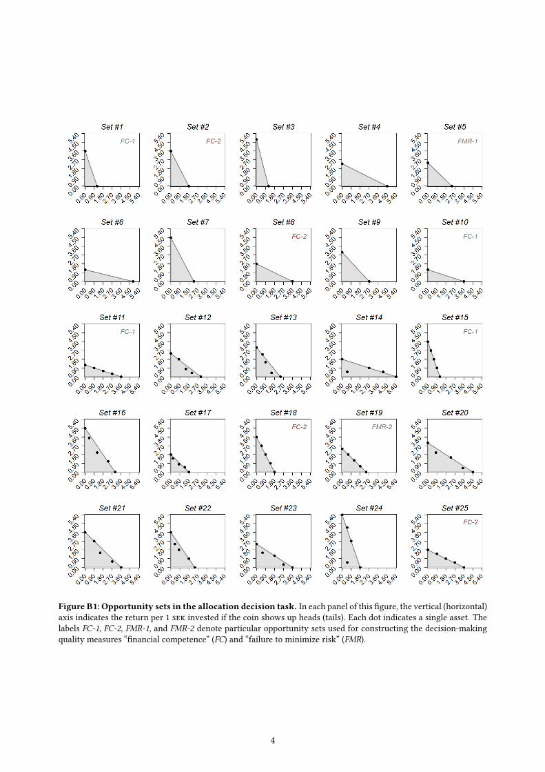
Figure B1: Opportunity sets in the allocation decision task. In each panel of this �gure, the vertical (horizontal)axis indicates the return per 1 ��� invested if the coin shows up heads (tails). Each dot indicates a single asset. Thelabels FC-1, FC-2, FMR-1, and FMR-2 denote particular opportunity sets used for constructing the decision-makingquality measures “�nancial competence” (FC) and “failure to minimize risk” (FMR).

4

C. Decision-Making Quality Measures

In each opportunity set j œ {1, 2, . . . , 25}, each participant i is endowed with 100 ��� to be allocated onassets k œ {1, 2, . . . , 5}. Let ai,j,k denote the fraction of the endowment allocated on asset k such thatq

k ai,j,k = 1.

The return per ��� invested in asset k if the coin comes up heads is denoted as hj,k; the return per ���invested if it comes up tails is denoted as tj,k. Thus, the return of participant i’s allocation in opportunityset j will either be

Hi,j =ÿ

k

ai,j,k · hj,k if the coin comes up heads, or

Ti,j =ÿ

k

ai,j,k · tj,k if the coin comes up tails.

Let the tuple xi,j = (Hi,j , Ti,j) denote the portfolio of participant i in opportunity set j. Following Bankset al. (2018), we de�ne four measures of decision-making quality: (i) violations of �rst order stochasticdominance (FOSD), (ii) violations of the generalized axiom of revealed preferences (GARP), (iii) �nancialcompetence (FC), and (iv) failure to minimize risk (FMR). Each of these measures is de�ned in detail below.

Expected Return. The expected portfolio return of participant i’s investment in opportunity set j, i.e.,the expected return from allocating the endowment on the available assets, is given by

ERi,j = Hi,j + Ti,j

2 .

Participant i’s mean expected return, ERi, is calculated as the average of ERi,j across 23 of the 25 oppor-tunity sets, as the expected returns are identical for all portfolios in the two remaining opportunity sets(set #5 and #19; see Table B1 and Figure B1), i.e., ERi = 1/23 ·

q23j=1 ERi,j .

Standard Deviation. As a measure of portfolio risk, we calculate the standard deviation of participanti’s portfolio in opportunity set j, i.e., the standard deviation of Hi,j and Ti,j occurring with a probabilityof 50% each:

SDi,j =Û

H2i,j + T

2i,j

2 ≠3

Hi,j + Ti,j

2

42.

The average portfolio risk for individual i, SDi, is de�ned as the mean standard deviation across all 25opportunity sets, i.e., SDi = 1/25 ·

q25j=1 SDi,j .

Violations of First Order Stochastic Dominance (FOSD). Suppose participant i chooses portfolioxi,j = (Hi,j ,Ti,j) in opportunity set j, i.e., an allocation returning Hi,j or Ti,j with 50% probability each,as illustrated in Figure C1. The �gure also depicts an alternative portfolio xÕ

i,j = (H Õi,j ,T

Õi,j). Apparently,

portfolio xÕi,j �rst order stochastically dominates xi,j because T

Õi,j = Hi,j and H

Õi,j > Ti,j .

Following Banks et al. (2018), we use the di�erence between the maximum expected return of a portfoliothat provides the same minimum payo� as the chosen portfolio and the expected return of the chosen

5

Tails

Heads

h⇤j

t⇤j

45� Line

xi,j

Ti,j

Hi,j

x0i,j

T0i,j = Hi,j

H0i,j > Ti,j

Figure C1: Violation of the principle of �rst order stochastic domi-nance (FOSD). The chosen portfolio xi,j is �rst order stochastically domi-nated by the alternative portfolio xÕ

i,j because TÕi,j = Hi,j and H

Õi,j > Ti,j .

That is, portfolio xÕi,j yields a higher expected return than xi,j while guar-

anteeing the same minimum payo�.

portfolio as a measure of how closely participant i’s choice in opportunity set j complies with the principleof FOSD (Hadar and Russell, 1969), i.e., FOSDi,j = (H Õ

i,j + TÕi,j) · 1/2 ≠ (Hi,j + Ti,j) · 1/2 in the example

depicted in Figure C1.

In general, given a chosen portfolio xi,j = (Hi,j ,Ti,j), let húj = max

khj,k be the maximum return across

all assets k if the coin comes up heads and túj = max

ktj,k if the the coin comes up tails. By investing the

fraction

w = min(Hi,j ,Ti,j)min(hú

j , túj )

on the asset paying min(húj , t

új ) and 0 ��� otherwise, and investing the fraction (1 ≠ w) on the asset

paying max(húj , t

új ) and 0 ��� otherwise, participant i maximizes the expected return but still guarantees

a minimum return of min(Hi,j ,Ti,j). Thus, our measure of FOSD is:

FOSDi,j =A

w ·min(hú

j , túj )

2 + (1 ≠ w) ·max(hú

j , túj )

2

B

≠ (Hi,j + Ti,j)2 .

To assess participant i’s average violations of FOSD, we average the measure over all choices, except forthe two opportunity sets for which any portfolio will yield the same expected returns (set #5 and #19; seeTable B1 and Figure B1), i.e., FOSDi = 1/23 ·

q23j=1 FOSDi,j .

6

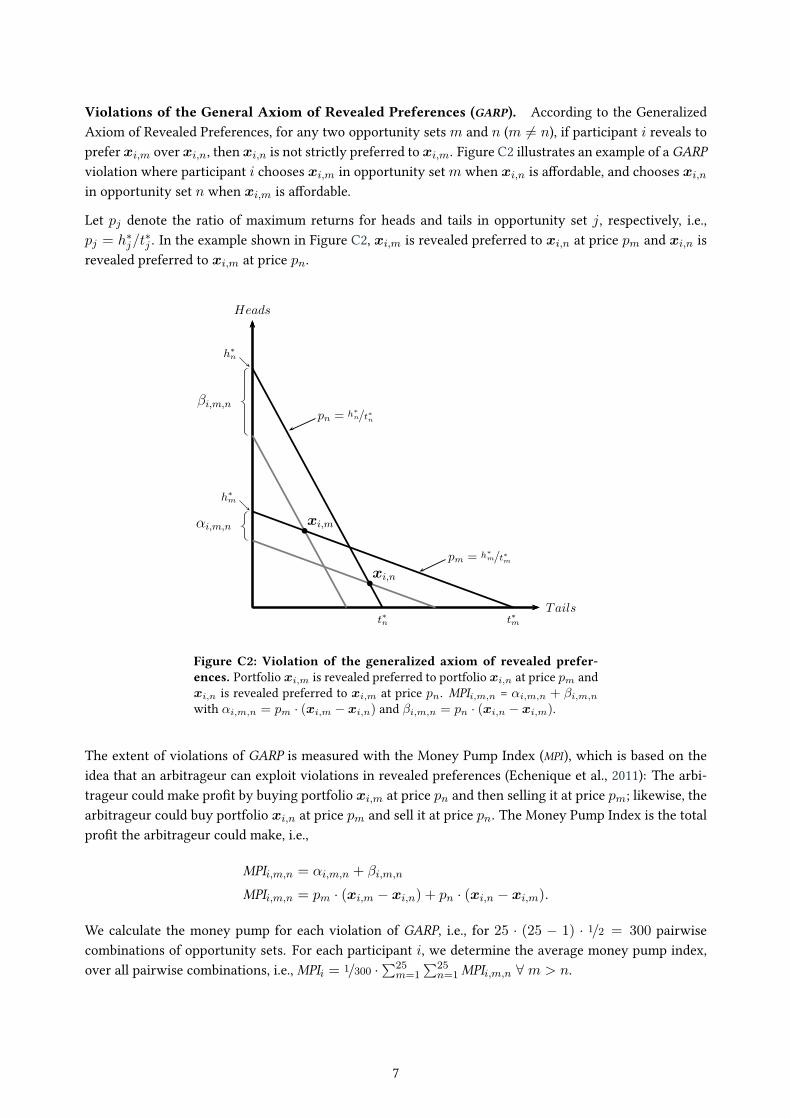
Violations of the General Axiom of Revealed Preferences (GARP). According to the GeneralizedAxiom of Revealed Preferences, for any two opportunity sets m and n (m ”= n), if participant i reveals toprefer xi,m over xi,n, then xi,n is not strictly preferred to xi,m. Figure C2 illustrates an example of a GARPviolation where participant i chooses xi,m in opportunity set m when xi,n is a�ordable, and chooses xi,n

in opportunity set n when xi,m is a�ordable.

Let pj denote the ratio of maximum returns for heads and tails in opportunity set j, respectively, i.e.,pj = h

új/t

új . In the example shown in Figure C2, xi,m is revealed preferred to xi,n at price pm and xi,n is

revealed preferred to xi,m at price pn.

Tails

Heads

pn = h⇤n/t⇤n

pm = h⇤m/t⇤m

h⇤m

t⇤m

xi,m

h⇤n

t⇤n

xi,n

↵i,m,n

�i,m,n

Figure C2: Violation of the generalized axiom of revealed prefer-ences. Portfolio xi,m is revealed preferred to portfolio xi,n at price pm andxi,n is revealed preferred to xi,m at price pn. MPIi,m,n = –i,m,n + —i,m,n

with –i,m,n = pm · (xi,m ≠ xi,n) and —i,m,n = pn · (xi,n ≠ xi,m).

The extent of violations of GARP is measured with the Money Pump Index (MPI), which is based on theidea that an arbitrageur can exploit violations in revealed preferences (Echenique et al., 2011): The arbi-trageur could make pro�t by buying portfolio xi,m at price pn and then selling it at price pm; likewise, thearbitrageur could buy portfolio xi,n at price pm and sell it at price pn. The Money Pump Index is the totalpro�t the arbitrageur could make, i.e.,

MPIi,m,n = –i,m,n + —i,m,n

MPIi,m,n = pm · (xi,m ≠ xi,n) + pn · (xi,n ≠ xi,m).

We calculate the money pump for each violation of GARP, i.e., for 25 · (25 ≠ 1) · 1/2 = 300 pairwisecombinations of opportunity sets. For each participant i, we determine the average money pump index,over all pairwise combinations, i.e., MPIi = 1/300 ·

q25m=1

q25n=1 MPIi,m,n ’ m > n.

7

Financial competence (FC). Four opportunity sets were identical in the two-asset- and the �ve-asset-frame, i.e., four sets were presented in both the two-asset- (sets #1, #2, #8, and #10) and the �ve-asset-frame(sets #11, #15, #18, and #25). Moreover, two of the four opportunity sets presented in the two-asset- and�ve-asset-frame, respectively, were constructed as mirror images of one another, i.e., only the payo�s forheads and tails were interchanged. Thus, two opportunity sets (denoted as FC1 and FC2 in Figure B1) weree�ectively presented four times each (#1 = #10 = #11 = #15 and #2 = #8 = #18 = #25).

Let J1 = {#1, #10, #11, #15} and J2 = {#2, #8, #18, #25}. Thus, J1 and J2 are sets containingidentical opportunity sets presented as mirror images and/or in the two-asset- or the �ve-asset-frame, re-spectively. The �nancial competence of individual i is de�ned as the average absolute di�erences betweenthe expected returns across the identical opportunity sets in J1 and J2, i.e.,

FCi = 112 ·

Q

aÿ

k,lœJ1

|ERi,k ≠ ERi,l| +ÿ

m,nœJ2

|ERi,m ≠ ERi,n|

R

b ’ k > l & m > n.

Note that our de�nition of FCi di�ers from the measure used by Banks et al. (2018), who average theabsolute di�erences in expected returns across the two frames, but not across the mirrored versions ofthe sets. However, the notion of “�nancial competence”, arguably, is not only re�ected by choosing thesame portfolio in an opportunity set presented in frames with varying complexity, but also by choosingthe same portfolio if heads and tails are interchanged.

Failure to minimize risk (FMR). In two opportunity sets (#5 and #19; see Figure B1), the expectedreturn per 1 ��� invested was the same for all assets k, such that all feasible portfolios will share thesame expected return. Choosing a fully-hedged portfolio (i.e., a zero-risk portfolio), thus, (second-order)dominates all other feasible portfolios in these two opportunity sets. The failure to minimize risk forsubject i in opportunity set j, FMRi,j , is measured as the standard deviation SDi,j of the particular portfolioallocation, which is then averaged over the two opportunity sets, i.e.,

FMRi = 12 ·

2ÿ

j=1SDi,j .

Decision-making quality index (DMQI). As a measure of decision-making quality, Banks et al. (2018)calculate the arithmetic mean of the four measures FOSD, MPI , FC, and FMR. We suggest an alternative ap-proach for two reasons. First, the measures on the subject level are not based on comparable aggregationlevels (for instance, the FMR index is constructed as the mean over two opportunity sets, whereas MPI is av-eraged across 300 pairwise combinations of opportunity sets). This implies that shortcomings in decision-making are weighted di�erently for each of the four indices. Second, there seems to be no obvious reasonwhy the four measures—which can di�er considerably in magnitude on an individual level—should beequally weighted.

Thus, rather than determining the mean of the four measure on the subject level, we utilize the pre-dicted values of a principal component analysis of the four measures to constitute the DMQI index foreach participant. The predictions of the principal component analysis summarized in Table C1 serve as

8

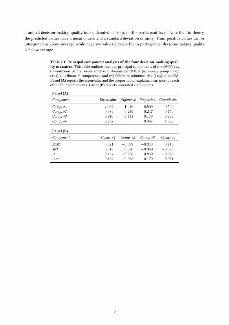
a uni�ed decision-making quality index, denoted as DMQI , on the participant level. Note that, in theory,the predicted values have a mean of zero and a standard deviation of unity. Thus, positive values can beinterpreted as above average while negative values indicate that a participants’ decision-making qualityis below average.

Table C1: Principal component analysis of the four decision-making qual-ity measures. This table outlines the four principal components of the DMQI , i.e.,(i) violations of �rst order stochastic dominance (FOSD), (ii) money pump index(MPI ), (iii) �nancial competence, and (iv) failure to minimize risk (FMR); n = 958.Panel (A) reports the eigenvalue and the proportion of explained variance for eachof the four components. Panel (B) reports unrotated components.

Panel (A)Component Eigenvalue Di�erence Proportion Cumulative

Comp. #1 2.034 1.046 0.509 0.509Comp. #2 0.989 0.279 0.247 0.756Comp. #3 0.710 0.444 0.178 0.933Comp. #4 0.267 . 0.067 1.000

Panel (B)Component Comp. #1 Comp. #2 Comp. #3 Comp. #4

FOSD 0.621 ≠0.099 ≠0.318 0.710MPI 0.618 0.026 ≠0.360 ≠0.698FC 0.457 ≠0.228 0.859 ≠0.048FMR 0.154 0.968 0.179 0.081

9

D. Questionnaires and Side Tasks

After the main experiment, participants were asked to answer a set of Likert items—all scaled from 0 (min-imum) to 10 (maximum)—which are summarized in Table D1 below. The questions on risk tolerance andpatience are based on Dohmen et al. (2011) and Falk et al. (2016, 2018); and the two statements addressingthe proneness to shift blame are based on the inventory introduced by Wilson et al. (1990). In addition tothe survey items reported in Table D1, participants were exposed to a hypothetical charitable giving settingbased on Falk et al. (2018), asking how much they would donate to a good cause if they had unexpectedlyreceived 10,000 ���.11 The 14 items were displayed on �ve separate screens: the �rst screen contained thequestions regarding risk preferences in general and their willingness to give up something today in orderto bene�t more in the future; the second screen included the item of risk tolerance in �nancial mattersas well as the three statements on trust; the third screen showed the hypothetical charitable giving task;the fourth screen comprised the two questions on blame shifting; and the �fth screen involved the �vequestions related to �nancial investments and the use of expertise.

Once the above questionnaires had been completed, participants answered eight questions allowing to de-termine their numeracy skills. As a measure of subjects’ numeracy, we use the number of correct answers.The numeracy task is based on the Rasch-validated inventory proposed by Weller et al. (2013). Two of theeight questions in the original set are well-known items from the Cognitive Re�ection Test (CRT) intro-duced by Frederick (2005). Since this three-item test has been widely spread on the Internet, many peoplewill know the questions and the corresponding answers. Therefore, the two items on cognitive re�ectionskills have been replaced by items from the CRT proposed by Toplak et al. (2014). For answering the eightquestions, participants faced a time constraint of four minutes. Since the items, by construction of the test,di�er considerably in di�culty, the order of the questions has been randomized to avoid systematic e�ectsarising from the time constraint. The questions used in the numeracy task are listed in Table D2.

After submitting their answers to the numeracy questions, participants were asked to self-assess theirperformance in the task in two di�erent ways: (i) “How many of the eight questions you answered onthe previous screen did you answer correctly?” (0 to 8), and (ii) “Compared to a random sample of theSwedish population, how did you score in terms of correct answers? Please estimate your position in theranking.” (Top 10%, Top 20%, . . . , Bottom 20%, Bottom 10%). While the �rst question allows for determin-ing participants’ overestimation of their own skills (as the di�erence between their estimates and actualperformance), the second question allows for quantifying subjects’ tendency to “overplace” their perfor-mance relative to others. Question (ii) asks participants to evaluate their performance relative to a randomsample of the Swedish population. However, our sample is not representative with respect to the levelof education due to self-selection e�ects. For this reason we take a detour to derive a sensible measureof overplacement: The validated inventory proposed by Weller et al. (2013) is constructed in such a waythat scores are approximately normally distributed among a general population sample. The fact that thenumeracy scores in our general population sample are signi�cantly di�erent from a normal distribution(Shapiro-Wilk-Test; W = 0.987, p < 0.001, n = 550) somewhat con�rms our conjecture of a self-selectione�ect in our sample. Thus, in a �rst step, we draw random integers from a normal distribution with a meanof 4.07 and a standard deviation of 1.83, the �rst and second moment reported for Study 2 in Weller et al.(2013), validating their Rasch-based measure. In a second step, we determine the percentiles associatedwith each possible score between 0 and 8. Finally, we deduct the percentile (from the sampled normal

11 The question was presented to participants as follows: “Imagine the following situation: Today you unexpectedly received10,000 ���. How much of this amount would you donate to a good cause?”

10

distribution) corresponding to participants’ numeracy score from their estimated decile, i.e., their answerto question (ii), to assess the degree of participants’ overplacement.12 As a �nal task of the experiment,participants were asked to answer six single-choice questions based on van Rooij et al. (2011), allowing todetermine their �nancial literacy. In particular, three of the questions stem from their basic literacy inven-tory (Q1–Q3, corresponding to (2), (3), and (5) in van Rooij et al. (2011)), and three questions are based onthe advanced literacy inventory (Q4–Q6, corresponding to (12), (16), and (7) in van Rooij et al. (2011)). Asan index of �nancial literacy, we use the sum of participants’ correct answers. The questions used in the�nancial literacy task are depicted in Table D3.

Descriptive results relating to the questionnaires are provided in Table E5 and Figures E1 and E2; summaryresults of the side experiments on numeracy skills, �nancial literacy, and the two measures of overcon�-dence are provided in Table E6 and Figures E3 and E4 in Appendix E.

12 As we ask participants to estimate their performance relative to the general population in deciles rather than percentiles, we usethe minimum di�erence to either of the bounds of the interval they implicitly provide as our measure of overestimation. That is,if the percentile (from the sampled normal distribution) lies within the interval subjects estimate, the measure takes value 0; ifthe percentile is smaller than the lower bound (upper bound) of the estimated interval, we evaluate the percentile to the lowerbound (upper bound) of the interval.

11

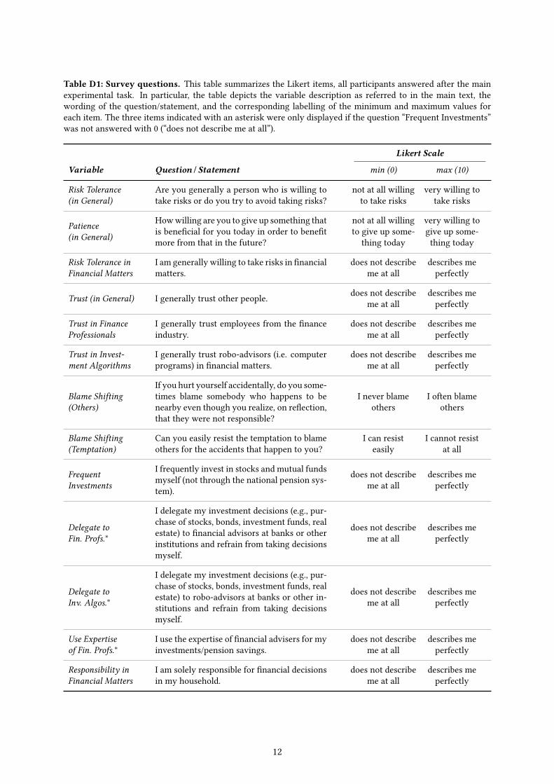
Table D1: Survey questions. This table summarizes the Likert items, all participants answered after the mainexperimental task. In particular, the table depicts the variable description as referred to in the main text, thewording of the question/statement, and the corresponding labelling of the minimum and maximum values foreach item. The three items indicated with an asterisk were only displayed if the question “Frequent Investments”was not answered with 0 (“does not describe me at all”).

Likert Scale

Variable Question / Statement min (0) max (10)

Risk Tolerance(in General)

Are you generally a person who is willing totake risks or do you try to avoid taking risks?

not at all willingto take risks

very willing totake risks

Patience(in General)

Howwilling are you to give up something thatis bene�cial for you today in order to bene�tmore from that in the future?

not at all willingto give up some-

thing today

very willing togive up some-thing today

Risk Tolerance inFinancial Matters

I am generally willing to take risks in �nancialmatters.

does not describeme at all

describes meperfectly

Trust (in General) I generally trust other people. does not describeme at all

describes meperfectly

Trust in FinanceProfessionals

I generally trust employees from the �nanceindustry.

does not describeme at all

describes meperfectly

Trust in Invest-ment Algorithms

I generally trust robo-advisors (i.e. computerprograms) in �nancial matters.

does not describeme at all

describes meperfectly

Blame Shifting(Others)

If you hurt yourself accidentally, do you some-times blame somebody who happens to benearby even though you realize, on re�ection,that they were not responsible?

I never blameothers

I often blameothers

Blame Shifting(Temptation)

Can you easily resist the temptation to blameothers for the accidents that happen to you?

I can resisteasily

I cannot resistat all

FrequentInvestments

I frequently invest in stocks and mutual fundsmyself (not through the national pension sys-tem).

does not describeme at all

describes meperfectly

Delegate toFin. Profs.ú

I delegate my investment decisions (e.g., pur-chase of stocks, bonds, investment funds, realestate) to �nancial advisors at banks or otherinstitutions and refrain from taking decisionsmyself.

does not describeme at all

describes meperfectly

Delegate toInv. Algos.ú

I delegate my investment decisions (e.g., pur-chase of stocks, bonds, investment funds, realestate) to robo-advisors at banks or other in-stitutions and refrain from taking decisionsmyself.

does not describeme at all

describes meperfectly

Use Expertiseof Fin. Profs.ú

I use the expertise of �nancial advisers for myinvestments/pension savings.

does not describeme at all

describes meperfectly

Responsibility inFinancial Matters

I am solely responsible for �nancial decisionsin my household.

does not describeme at all

describes meperfectly

12

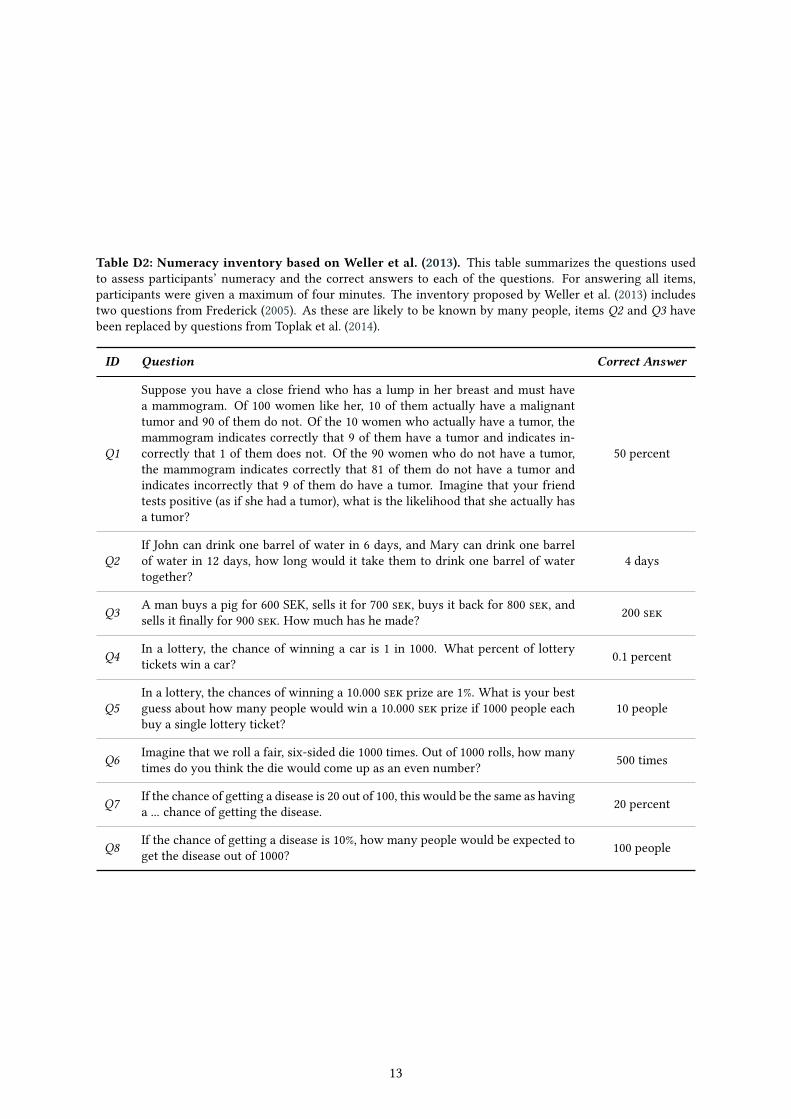
Table D2: Numeracy inventory based on Weller et al. (2013). This table summarizes the questions usedto assess participants’ numeracy and the correct answers to each of the questions. For answering all items,participants were given a maximum of four minutes. The inventory proposed by Weller et al. (2013) includestwo questions from Frederick (2005). As these are likely to be known by many people, items Q2 and Q3 havebeen replaced by questions from Toplak et al. (2014).

ID Question Correct Answer

Q1

Suppose you have a close friend who has a lump in her breast and must havea mammogram. Of 100 women like her, 10 of them actually have a malignanttumor and 90 of them do not. Of the 10 women who actually have a tumor, themammogram indicates correctly that 9 of them have a tumor and indicates in-correctly that 1 of them does not. Of the 90 women who do not have a tumor,the mammogram indicates correctly that 81 of them do not have a tumor andindicates incorrectly that 9 of them do have a tumor. Imagine that your friendtests positive (as if she had a tumor), what is the likelihood that she actually hasa tumor?

50 percent

Q2If John can drink one barrel of water in 6 days, and Mary can drink one barrelof water in 12 days, how long would it take them to drink one barrel of watertogether?

4 days

Q3 A man buys a pig for 600 SEK, sells it for 700 ���, buys it back for 800 ���, andsells it �nally for 900 ���. How much has he made? 200 ���

Q4 In a lottery, the chance of winning a car is 1 in 1000. What percent of lotterytickets win a car? 0.1 percent

Q5In a lottery, the chances of winning a 10.000 ��� prize are 1%. What is your bestguess about how many people would win a 10.000 ��� prize if 1000 people eachbuy a single lottery ticket?

10 people

Q6 Imagine that we roll a fair, six-sided die 1000 times. Out of 1000 rolls, how manytimes do you think the die would come up as an even number? 500 times

Q7 If the chance of getting a disease is 20 out of 100, this would be the same as havinga ... chance of getting the disease. 20 percent

Q8 If the chance of getting a disease is 10%, how many people would be expected toget the disease out of 1000? 100 people

13

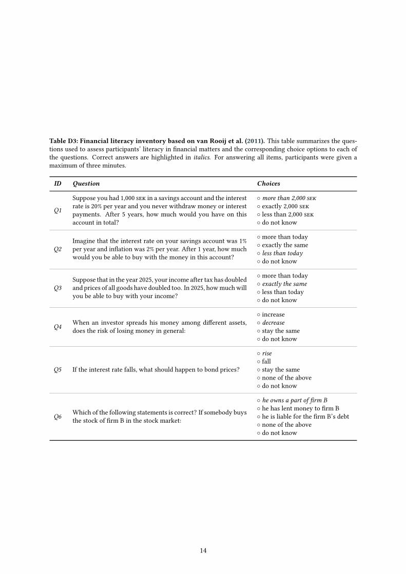
Table D3: Financial literacy inventory based on van Rooij et al. (2011). This table summarizes the ques-tions used to assess participants’ literacy in �nancial matters and the corresponding choice options to each ofthe questions. Correct answers are highlighted in italics. For answering all items, participants were given amaximum of three minutes.

ID Question Choices

Q1

Suppose you had 1,000 ��� in a savings account and the interestrate is 20% per year and you never withdraw money or interestpayments. After 5 years, how much would you have on thisaccount in total?

¶ more than 2,000 ���¶ exactly 2,000 ���¶ less than 2,000 ���¶ do not know

Q2Imagine that the interest rate on your savings account was 1%per year and in�ation was 2% per year. After 1 year, how muchwould you be able to buy with the money in this account?

¶ more than today¶ exactly the same¶ less than today¶ do not know

Q3Suppose that in the year 2025, your income after tax has doubledand prices of all goods have doubled too. In 2025, howmuchwillyou be able to buy with your income?

¶ more than today¶ exactly the same¶ less than today¶ do not know

Q4 When an investor spreads his money among di�erent assets,does the risk of losing money in general:

¶ increase¶ decrease¶ stay the same¶ do not know

Q5 If the interest rate falls, what should happen to bond prices?

¶ rise¶ fall¶ stay the same¶ none of the above¶ do not know

Q6 Which of the following statements is correct? If somebody buysthe stock of �rm B in the stock market:

¶ he owns a part of �rm B¶ he has lent money to �rm B¶ he is liable for the �rm B’s debt¶ none of the above¶ do not know

14

E. Descriptive Results

In the following, we present a set of descriptive results for all measures elicited in the experiment. Manyof these variables only enter our analyses as controls. Yet, while several results presented below back upour main �ndings, we also deem it interesting to compare our two subject pools—participants from thegeneral population and professionals from the �nance industry—along these measures.

Response rate analysis and self-selection. For the �nance professionals group, the response rateanalysis shows that men responded to a greater extent than women, and that �nance individuals in theage group 45–59 years responded to a slightly lesser extent than other ages. Furthermore, the non-responseanalysis shows that those with the lowest income responded to a somewhat higher degree compared to theothers, and that those with a post-secondary education level of three years or more responded to greaterextent than others. In the case of country of birth, the response rate was slightly higher for those born inSweden compared to other countries. In the �nance group there was a certain di�erence between the dif-ferent job codes where the response frequency was slightly lower (5%) in the group of traders and portfoliomanagers (job code “2414”) compared with analysts and advisors (code “2413”) and brokers (code“3311”)(6.4%).

For the general population group, the response rate analysis shows similar patterns regarding gender,i.e., men responded to a greater extent than women. The response rate was lowest among the elderly.Furthermore, the response rate analysis indicates that those with the lowest and highest income respondedto a somewhat higher extent compared to other income groups. When it comes to the level of education,those with a post-secondary education of three years or more tend to be over-represented in our sample.In the case of country of birth, the response rate was slightly higher for the ones born in Sweden comparedto other countries.

A detailed summary of participants demographics compared to the characteristics of the sample invitedis presented in Table E1. In particular, Table E1 reports the number of respondents and non-respondentsper category of several socio-demographic characteristics, separated for both samples, as reported by SCB.Moreover, we report‰

2-tests comparingwhether participants in our samples di�er signi�cantly from thosewho have been invited by SCB but did not participate in the experiment. As discussed in Appendix A, wereport self-selection e�ects in terms of gender, age, country of birth, income, and education for the generalpopulation sample, and self-selection e�ects with respect to gender, age, and education for the �nanceprofessionals sample. For a discussion of how this translates into the decision-making quality measures,see the discussion below.

Decision-making qualitymeasures. Table E2 reports summary statistics of the decision-making qual-ity measures derived from the main task (see Appendix B and C for details), separated for the generalpopulation sample and the �nance professionals. Since we conjecture that the varying incentive structurebetween treatments in the �nance professionals’ sample gives rise to di�erences in decision-making qual-ity, the summary statistics are separated for the three treatments. Notably, all measures—except for theindex capturing �nancial competence (FC)—are considerably left-skewed for both samples and across alltreatments.

15

On average, decision-making quality is remarkably high, both for �nance professionals and the generalpopulation sample. Comparing the means of the decision-making measures in our samples to the meansreported by Banks et al. (2018)13 shows that our general population sample performs signi�cantly betterthan the participants in Banks et al. (2018) in all four measures (two-sample t-tests; p < 0.001 for all com-parisons). This, too, indicates that our sample is highly sophisticated, which might be one of the reasonswhy we do not �nd strong di�erences in decision-making quality between the �nance professionals andthe general population in our results.

13 Banks et al. (2018) report the following means (m) and standard deviations (sd) for their (“pre-reform”) general population sample(n = 1,416) from the US: m = ≠$3.68, sd = $1.93 (FOSD); m = ≠$2.77, sd = $3.87 (MPI ); m = ≠$6.98, sd = $3.97 (FC); andm = ≠$3.32, sd = $4.91 (FMR). Two pivotal di�erences need to be taken into account, to come up with sensible comparisons:(i) in Banks et al. (2018), participants receive an endowment of of $25 to be allocated on the assets; in contrast, in our setting,participants were endowedwith 100 ���; (ii) all assets’ payo�s fromBanks et al. (2018) have beenmultiplied by a factor of 1.5 in ourexperiment. Thus, multiplying the means and standard deviations reported by Banks et al. (2018) by a factor of 100/25 · 1.5 = 6provides sensible benchmarks for the decision-making quality measures in our setting. In particular, the summary statisticsprovided in Table E2 can be compared to the following adjusted values from Banks et al. (2018): m = ≠$22.08, sd = $11.58(FOSD); m = ≠$16.62, sd = $23.22 (MPI ); m = ≠$41.88, sd = $23.82 (FC); and m = ≠$19.92, sd = $29.46 (FMR).

16

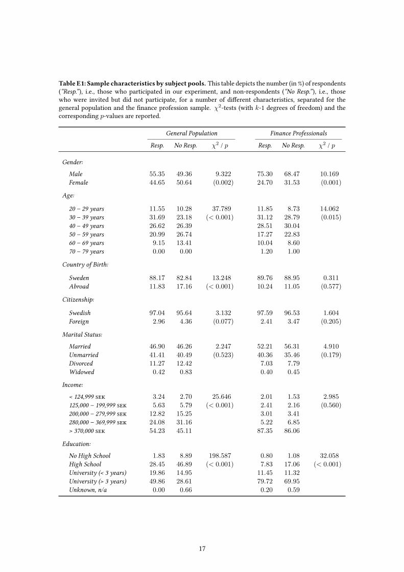
Table E1: Sample characteristics by subject pools. This table depicts the number (in %) of respondents(“Resp.” ), i.e., those who participated in our experiment, and non-respondents (“No Resp.” ), i.e., thosewho were invited but did not participate, for a number of di�erent characteristics, separated for thegeneral population and the �nance profession sample. ‰

2-tests (with k-1 degrees of freedom) and thecorresponding p-values are reported.

General Population Finance Professionals

Resp. No Resp. ‰2 / p Resp. No Resp. ‰

2 / p

Gender:

Male 55.35 49.36 9.322 75.30 68.47 10.169Female 44.65 50.64 (0.002) 24.70 31.53 (0.001)

Age:

20 – 29 years 11.55 10.28 37.789 11.85 8.73 14.06230 – 39 years 31.69 23.18 (< 0.001) 31.12 28.79 (0.015)40 – 49 years 26.62 26.39 28.51 30.0450 – 59 years 20.99 26.74 17.27 22.8360 – 69 years 9.15 13.41 10.04 8.6070 – 79 years 0.00 0.00 1.20 1.00

Country of Birth:

Sweden 88.17 82.84 13.248 89.76 88.95 0.311Abroad 11.83 17.16 (< 0.001) 10.24 11.05 (0.577)

Citizenship:

Swedish 97.04 95.64 3.132 97.59 96.53 1.604Foreign 2.96 4.36 (0.077) 2.41 3.47 (0.205)

Marital Status:

Married 46.90 46.26 2.247 52.21 56.31 4.910Unmarried 41.41 40.49 (0.523) 40.36 35.46 (0.179)Divorced 11.27 12.42 7.03 7.79Widowed 0.42 0.83 0.40 0.45

Income:

< 124,999 ��� 3.24 2.70 25.646 2.01 1.53 2.985125,000 – 199,999 ��� 5.63 5.79 (< 0.001) 2.41 2.16 (0.560)200,000 – 279,999 ��� 12.82 15.25 3.01 3.41280,000 – 369,999 ��� 24.08 31.16 5.22 6.85> 370,000 ��� 54.23 45.11 87.35 86.06

Education:

No High School 1.83 8.89 198.587 0.80 1.08 32.058High School 28.45 46.89 (< 0.001) 7.83 17.06 (< 0.001)University (< 3 years) 19.86 14.95 11.45 11.32University (> 3 years) 49.86 28.61 79.72 69.95Unknown, n/a 0.00 0.66 0.20 0.59

17

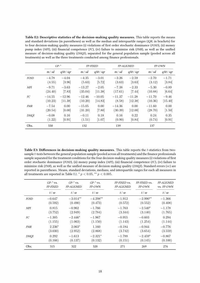
Table E2: Descriptive statistics of the decision-making quality measures. This table reports the meansand standard deviations (in parentheses) as well as the median and interquartile ranges (IQR; in brackets) forto four decision-making quality measures (i) violations of �rst order stochastic dominance (FOSD), (ii) moneypump index (MPI ), (iii) �nancial competence (FC), (iv) failure to minimize risk (FMR), as well as the uni�edmeasure of decision-making quality (DMQI ), separated for the general population sample (pooled across alltreatments) as well as the three treatments conducted among �nance professionals.

GP-* FP-FIXED FP-ALIGNED FP-OWN

m / sd q50 / iqr m / sd q50 / iqr m / sd q50 / iqr m / sd q50 / iqr

FOSD ≠4.78 ≠4.04 ≠4.35 ≠3.01 ≠3.26 ≠2.59 ≠2.70 ≠1.71(4.55) [3.96] (5.63) [5.72] (3.63) [3.63] (3.12) [3.84]

MPI ≠9.71 ≠3.63 ≠13.27 ≠2.05 ≠7.38 ≠2.33 ≠5.30 ≠0.89(24.40) [7.83] (35.04) [11.38] (17.61) [7.44] (10.88) [6.64]

FC ≠14.55 ≠12.96 ≠12.46 ≠10.05 ≠11.37 ≠11.28 ≠11.70 ≠9.46(10.23) [11.38] (10.20) [14.83] (8.58) [12.38] (10.36) [15.40]

FMR ≠7.54 0.00 ≠15.05 0.00 ≠14.36 0.00 ≠11.60 0.00(20.54) [0.00] (31.20) [7.80] (30.39) [12.00] (28.70) [1.50]

DMQI ≠0.08 0.16 ≠0.11 0.18 0.16 0.22 0.24 0.35(1.22) [0.91] (1.51) [1.07] (0.90) [0.84] (0.74) [0.91]

Obs. 550 132 139 137

Table E3: Di�erences in decision-making quality measures. This table reports the t-statistics from two-sample t-tests between the general population sample (pooled across all treatments) and the �nance professionalssample separated for the treatment conditions for the four decision-making quality measures (i) violations of �rstorder stochastic dominance (FOSD), (ii) money pump index (MPI ), (iii) �nancial competence (FC), (iv) failure tominimize risk (FMR), as well as the uni�ed measure of decision-making quality (DMQI ). Standard errors (se) arereported in parentheses. Means, standard deviations, medians, and interquartile ranges for each all measures inall treatments are reported in Table E2. * p < 0.05, ** p < 0.005.

GP-* vs.FP-FIXED

GP-* vs.FP-ALIGNED

GP-* vs.FP-OWN

FP-FIXED vs.FP-ALIGNED

FP-FIXED vs.FP-OWN

FP-ALIGNEDvs. FP-OWN

t / se t / se t / se t / se t / se t / se

FOSD ≠0.647 ≠3.014** ≠4.298** ≠1.912 ≠2.990** ≠1.366(0.592) (0.490) (0.473) (0.572) (0.552) (0.408)

MPI 0.815 ≠0.962 ≠1.766 ≠1.763 ≠2.540* ≠1.178(3.752) (2.949) (2.784) (3.344) (3.140) (1.765)

FC ≠1.305 ≠2.446* ≠1.967 ≠0.955 ≠0.603 0.294(1.155) (1.063) (1.150) (1.143) (1.254) (1.144)

FMR 2.236* 2.063* 1.160 ≠0.184 ≠0.944 ≠0.776(3.030) (2.952) (2.868) (3.742) (3.654) (3.559)

DMQI 0.292 ≠1.613 ≠2.321* ≠1.788 ≠2.459* ≠0.867(0.166) (0.137) (0.132) (0.151) (0.145) (0.100)

Obs. 315 322 320 271 269 276

18

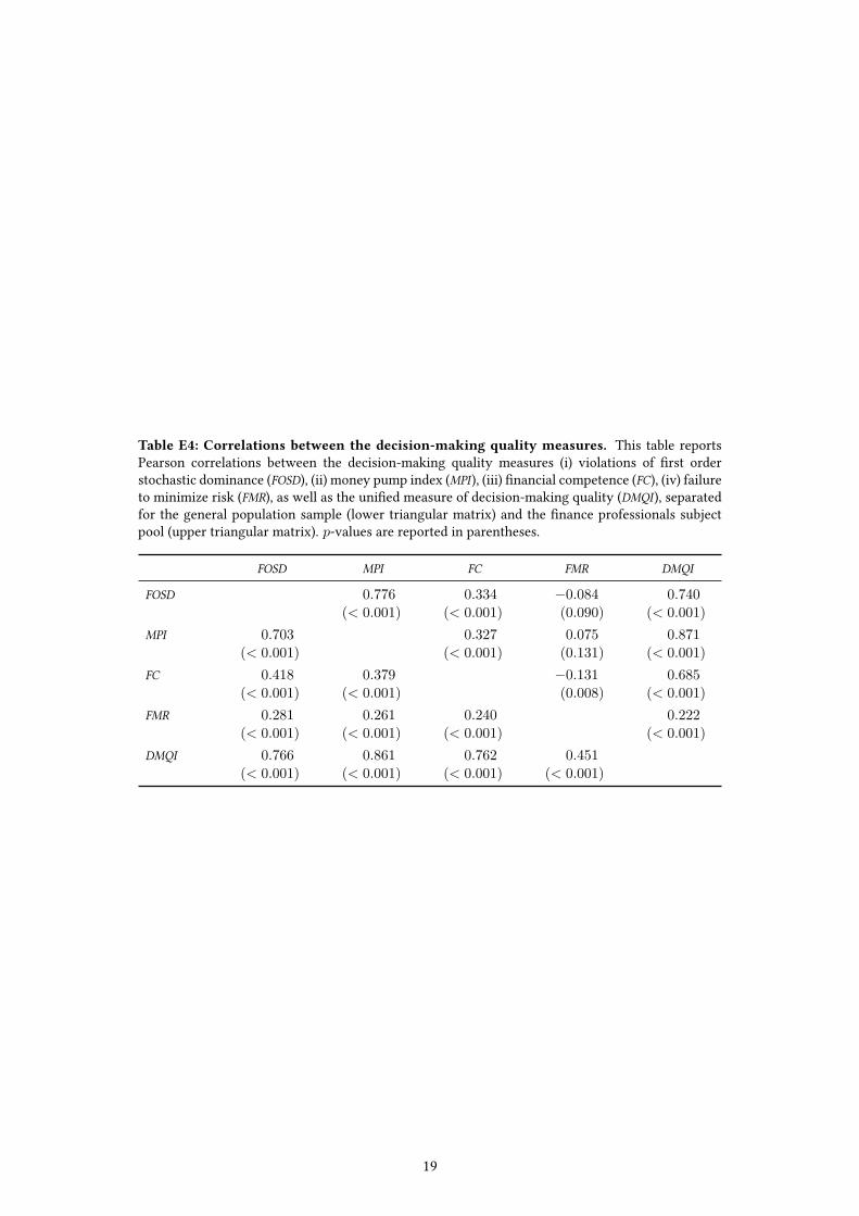
Table E4: Correlations between the decision-making quality measures. This table reportsPearson correlations between the decision-making quality measures (i) violations of �rst orderstochastic dominance (FOSD), (ii) money pump index (MPI ), (iii) �nancial competence (FC), (iv) failureto minimize risk (FMR), as well as the uni�ed measure of decision-making quality (DMQI ), separatedfor the general population sample (lower triangular matrix) and the �nance professionals subjectpool (upper triangular matrix). p-values are reported in parentheses.

FOSD MPI FC FMR DMQI

FOSD 0.776 0.334 ≠0.084 0.740(< 0.001) (< 0.001) (0.090) (< 0.001)

MPI 0.703 0.327 0.075 0.871(< 0.001) (< 0.001) (0.131) (< 0.001)

FC 0.418 0.379 ≠0.131 0.685(< 0.001) (< 0.001) (0.008) (< 0.001)

FMR 0.281 0.261 0.240 0.222(< 0.001) (< 0.001) (< 0.001) (< 0.001)

DMQI 0.766 0.861 0.762 0.451(< 0.001) (< 0.001) (< 0.001) (< 0.001)

19

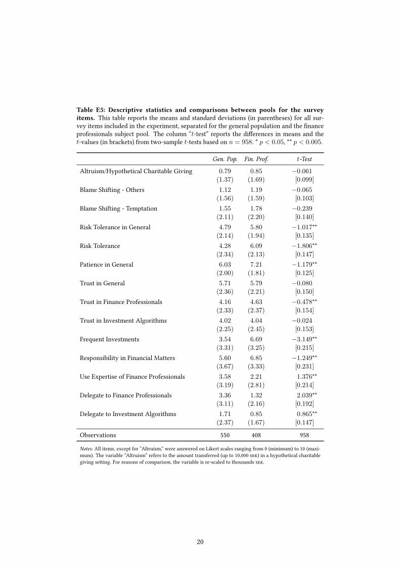
Table E5: Descriptive statistics and comparisons between pools for the surveyitems. This table reports the means and standard deviations (in parentheses) for all sur-vey items included in the experiment, separated for the general population and the �nanceprofessionals subject pool. The column “t-test” reports the di�erences in means and thet-values (in brackets) from two-sample t-tests based on n = 958. * p < 0.05, ** p < 0.005.

Gen. Pop. Fin. Prof. t-Test

Altruism/Hypothetical Charitable Giving 0.79 0.85 ≠0.061(1.37) (1.69) [0.099]

Blame Shifting - Others 1.12 1.19 ≠0.065(1.56) (1.59) [0.103]

Blame Shifting - Temptation 1.55 1.78 ≠0.239(2.11) (2.20) [0.140]

Risk Tolerance in General 4.79 5.80 ≠1.017**(2.14) (1.94) [0.135]

Risk Tolerance 4.28 6.09 ≠1.806**(2.34) (2.13) [0.147]

Patience in General 6.03 7.21 ≠1.179**(2.00) (1.81) [0.125]

Trust in General 5.71 5.79 ≠0.080(2.36) (2.21) [0.150]

Trust in Finance Professionals 4.16 4.63 ≠0.478**(2.33) (2.37) [0.154]

Trust in Investment Algorithms 4.02 4.04 ≠0.024(2.25) (2.45) [0.153]

Frequent Investments 3.54 6.69 ≠3.149**(3.31) (3.25) [0.215]

Responsibility in Financial Matters 5.60 6.85 ≠1.249**(3.67) (3.33) [0.231]

Use Expertise of Finance Professionals 3.58 2.21 1.376**(3.19) (2.81) [0.214]

Delegate to Finance Professionals 3.36 1.32 2.039**(3.11) (2.16) [0.192]

Delegate to Investment Algorithms 1.71 0.85 0.865**(2.37) (1.67) [0.147]

Observations 550 408 958

Notes: All items, except for “Altruism,” were answered on Likert scales ranging from 0 (minimum) to 10 (maxi-mum). The variable “Altruism” refers to the amount transferred (up to 10,000 ���) in a hypothetical charitablegiving setting. For reasons of comparison, the variable is re-scaled to thousands ���.

20

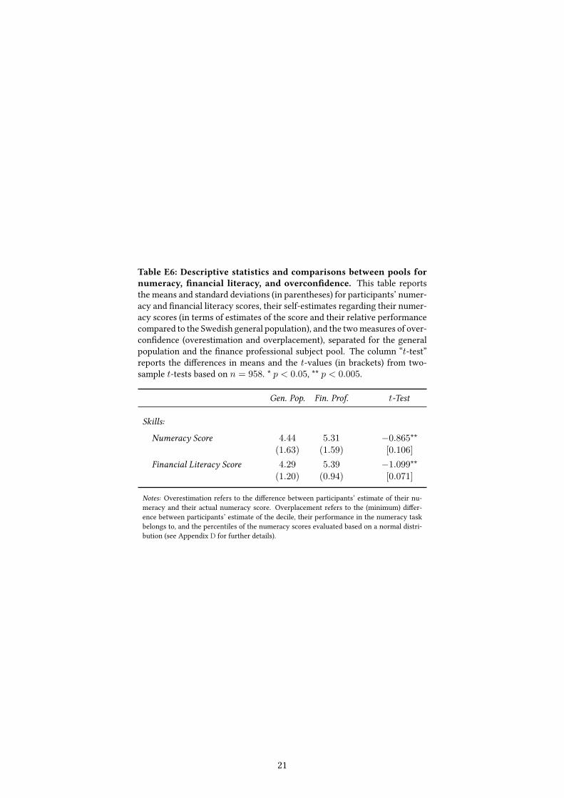
Table E6: Descriptive statistics and comparisons between pools fornumeracy, �nancial literacy, and overcon�dence. This table reportsthe means and standard deviations (in parentheses) for participants’ numer-acy and �nancial literacy scores, their self-estimates regarding their numer-acy scores (in terms of estimates of the score and their relative performancecompared to the Swedish general population), and the twomeasures of over-con�dence (overestimation and overplacement), separated for the generalpopulation and the �nance professional subject pool. The column “t-test”reports the di�erences in means and the t-values (in brackets) from two-sample t-tests based on n = 958. * p < 0.05, ** p < 0.005.

Gen. Pop. Fin. Prof. t-Test

Skills:

Numeracy Score 4.44 5.31 ≠0.865**(1.63) (1.59) [0.106]

Financial Literacy Score 4.29 5.39 ≠1.099**(1.20) (0.94) [0.071]

Notes: Overestimation refers to the di�erence between participants’ estimate of their nu-meracy and their actual numeracy score. Overplacement refers to the (minimum) di�er-ence between participants’ estimate of the decile, their performance in the numeracy taskbelongs to, and the percentiles of the numeracy scores evaluated based on a normal distri-bution (see Appendix D for further details).

21

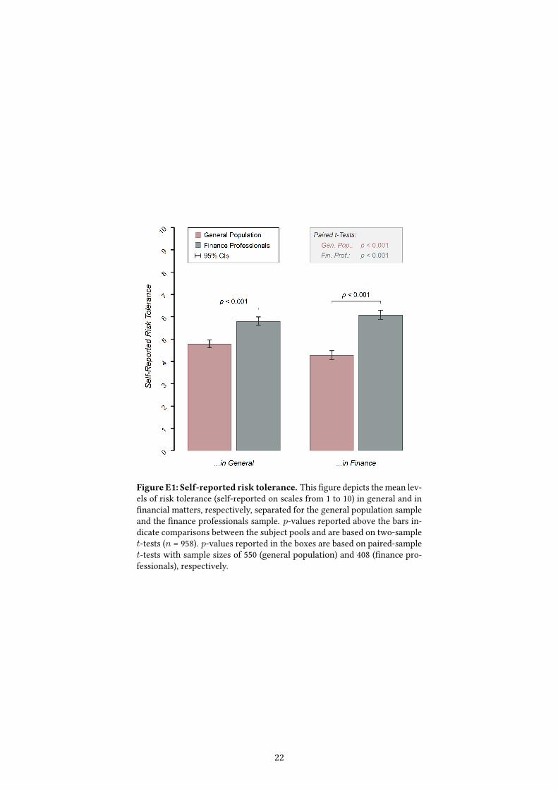
Figure E1: Self-reported risk tolerance. This �gure depicts themean lev-els of risk tolerance (self-reported on scales from 1 to 10) in general and in�nancial matters, respectively, separated for the general population sampleand the �nance professionals sample. p-values reported above the bars in-dicate comparisons between the subject pools and are based on two-samplet-tests (n = 958). p-values reported in the boxes are based on paired-samplet-tests with sample sizes of 550 (general population) and 408 (�nance pro-fessionals), respectively.

22

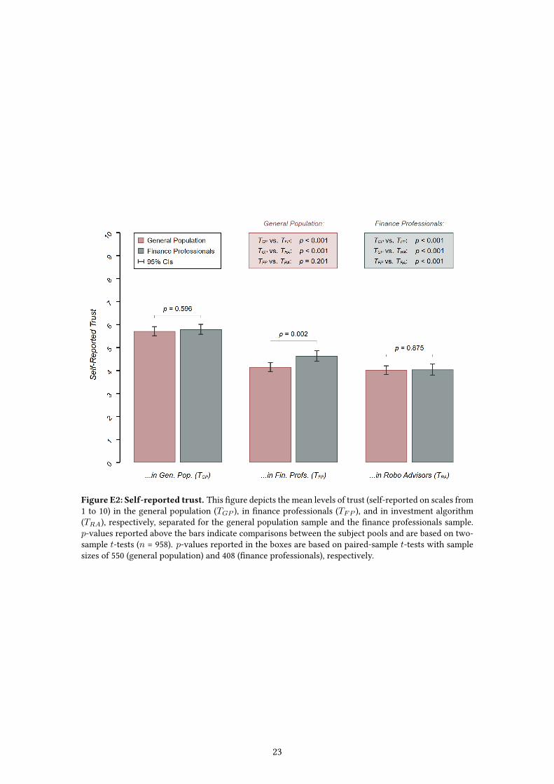
Figure E2: Self-reported trust. This �gure depicts the mean levels of trust (self-reported on scales from1 to 10) in the general population (TGP ), in �nance professionals (TF P ), and in investment algorithm(TRA), respectively, separated for the general population sample and the �nance professionals sample.p-values reported above the bars indicate comparisons between the subject pools and are based on two-sample t-tests (n = 958). p-values reported in the boxes are based on paired-sample t-tests with samplesizes of 550 (general population) and 408 (�nance professionals), respectively.

23

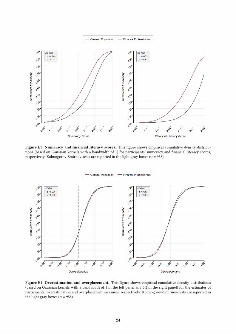
Figure E3: Numeracy and �nancial literacy scores. This �gure shows empirical cumulative density distribu-tions (based on Gaussian kernels with a bandwidth of 1) for participants’ numeracy and �nancial literacy scores,respectively. Kolmogorov-Smirnov-tests are reported in the light gray boxes (n = 958).

Figure E4: Overestimation and overplacement. This �gure shows empirical cumulative density distributions(based on Gaussian kernels with a bandwidth of 1 in the left panel and 0.2 in the right panel) for the estimates ofparticipants’ overestimation and overplacement measures, respectively. Kolmogorov-Smirnov-tests are reported inthe light gray boxes (n = 958).

24

F. Descriptives and Analyses of Time Spent

In the following, we examine the time spent per experimental task in the online experiment. Throughoutthe analysis, we truncate the time spent per task at the 99% percentile to avoid that outliers distort theresults. In particular, for each task, durations exceeding this threshold are replaced by the value of the99% percentile. Descriptive statistics of the time spent per task, separated for the general population andthe �nance professionals subject pools, are presented in Table F1. On average, the times spent in theexperimental tasks appear to be su�ciently long to be con�dent that participants in both samples tookthe experiment very seriously, which is also con�rmed by the high levels of decision-making quality (seeAppendix C for details). Di�erences in the time spent between the two pools are reported in Table F2.

With respect to the main task, we examine learning e�ects by means of ordinary least squares regressionsof the time spent on the 25 decisions on a linear time trend (with standard errors clustered at the subjectlevel). The regressions reveal that the time spent per decision decreases with the progressing round num-bers, in the decisions with both two and �ve assets, respectively. For the �rst two-asset item, participantsfrom the general population take, on average, 57.1 seconds; for the subsequent decisions, the time spent,on average, decreases by 5.1 seconds per item (t(548) = 13.916, p < 0.001, n = 5,500). Finance pro-fessionals take, on average, 72.7 seconds for the �rst two-asset decision; for the following nine decisionswith two assets, the time spent, on average, decreases by 6.5 seconds per item (t(406) = 8.776, p < 0.001,n = 6,120). Likewise, learning is observed for consecutive investment decisions with �ve assets. Forthe �rst �ve-asset item, participants from the general population take, on average, 3.5 minutes; for thesubsequent decisions, the time spent, on average, decreases by 13.1 seconds per item (t(548) = 2.065,p = 0.039, n = 5,500). Finance professionals take, on average, 2.6 minutes for the �rst �ve-asset decision;for the following fourteen decisions with �ve assets, the time spent, on average, decreases by 7.7 secondsper item (t(406) = 2.844, p = 0.005, n = 6,120).

In addition, we investigate whether decision-making quality is systematically a�ected by time participantstake to decide on the 25 investment decisions. Notably, ordinary least squares regression of the decision-making quality index (DMQI) on the time spent on the investment task (i.e., the sum of the time spent in theinvestment task with two and �ve assets) reveal that subjects’ proneness to poor investment decisions isnot signi�cantly driven by the time they spend on each decision, neither in the general population sample(— = 0.005, t(548) = 1.314, p = 0.189, n = 550), nor in the �nance professionals sample (— = 0.003,t(406) = 1.261, p = 0.208, n = 408).

25

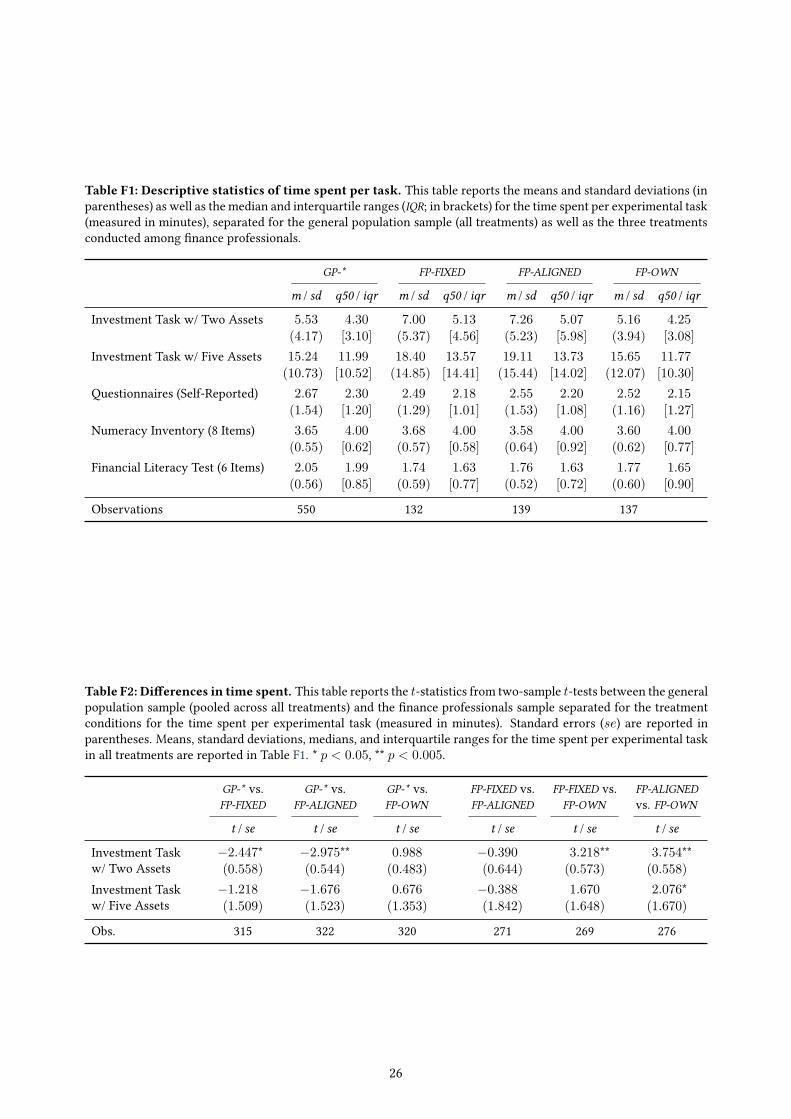
Table F1: Descriptive statistics of time spent per task. This table reports the means and standard deviations (inparentheses) as well as the median and interquartile ranges (IQR; in brackets) for the time spent per experimental task(measured in minutes), separated for the general population sample (all treatments) as well as the three treatmentsconducted among �nance professionals.

GP-* FP-FIXED FP-ALIGNED FP-OWN

m / sd q50 / iqr m / sd q50 / iqr m / sd q50 / iqr m / sd q50 / iqr

Investment Task w/ Two Assets 5.53 4.30 7.00 5.13 7.26 5.07 5.16 4.25(4.17) [3.10] (5.37) [4.56] (5.23) [5.98] (3.94) [3.08]

Investment Task w/ Five Assets 15.24 11.99 18.40 13.57 19.11 13.73 15.65 11.77(10.73) [10.52] (14.85) [14.41] (15.44) [14.02] (12.07) [10.30]

Questionnaires (Self-Reported) 2.67 2.30 2.49 2.18 2.55 2.20 2.52 2.15(1.54) [1.20] (1.29) [1.01] (1.53) [1.08] (1.16) [1.27]

Numeracy Inventory (8 Items) 3.65 4.00 3.68 4.00 3.58 4.00 3.60 4.00(0.55) [0.62] (0.57) [0.58] (0.64) [0.92] (0.62) [0.77]

Financial Literacy Test (6 Items) 2.05 1.99 1.74 1.63 1.76 1.63 1.77 1.65(0.56) [0.85] (0.59) [0.77] (0.52) [0.72] (0.60) [0.90]

Observations 550 132 139 137

Table F2: Di�erences in time spent. This table reports the t-statistics from two-sample t-tests between the generalpopulation sample (pooled across all treatments) and the �nance professionals sample separated for the treatmentconditions for the time spent per experimental task (measured in minutes). Standard errors (se) are reported inparentheses. Means, standard deviations, medians, and interquartile ranges for the time spent per experimental taskin all treatments are reported in Table F1. * p < 0.05, ** p < 0.005.

GP-* vs.FP-FIXED

GP-* vs.FP-ALIGNED

GP-* vs.FP-OWN

FP-FIXED vs.FP-ALIGNED

FP-FIXED vs.FP-OWN

FP-ALIGNEDvs. FP-OWN

t / se t / se t / se t / se t / se t / se

Investment Taskw/ Two Assets

≠2.447* ≠2.975** 0.988 ≠0.390 3.218** 3.754**(0.558) (0.544) (0.483) (0.644) (0.573) (0.558)

Investment Taskw/ Five Assets

≠1.218 ≠1.676 0.676 ≠0.388 1.670 2.076*(1.509) (1.523) (1.353) (1.842) (1.648) (1.670)

Obs. 315 322 320 271 269 276

26

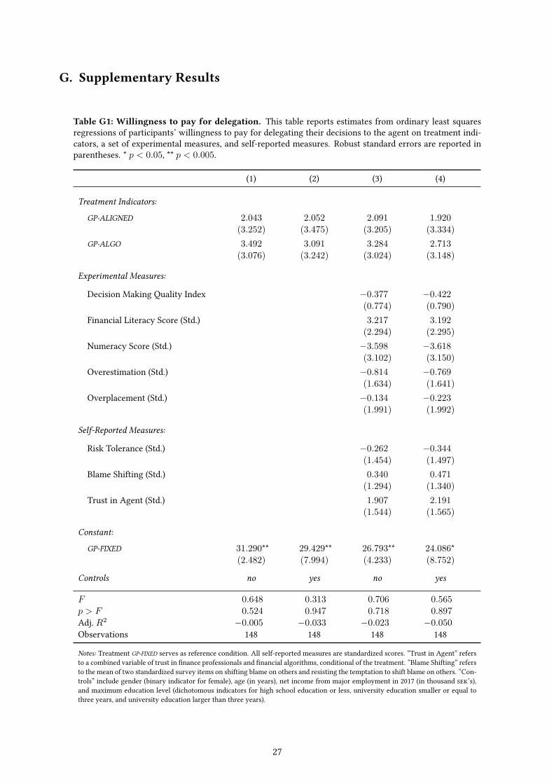
G. Supplementary Results

Table G1: Willingness to pay for delegation. This table reports estimates from ordinary least squaresregressions of participants’ willingness to pay for delegating their decisions to the agent on treatment indi-cators, a set of experimental measures, and self-reported measures. Robust standard errors are reported inparentheses. * p < 0.05, ** p < 0.005.

(1) (2) (3) (4)

Treatment Indicators:

GP-ALIGNED 2.043 2.052 2.091 1.920(3.252) (3.475) (3.205) (3.334)

GP-ALGO 3.492 3.091 3.284 2.713(3.076) (3.242) (3.024) (3.148)

Experimental Measures:

Decision Making Quality Index ≠0.377 ≠0.422(0.774) (0.790)

Financial Literacy Score (Std.) 3.217 3.192(2.294) (2.295)

Numeracy Score (Std.) ≠3.598 ≠3.618(3.102) (3.150)

Overestimation (Std.) ≠0.814 ≠0.769(1.634) (1.641)

Overplacement (Std.) ≠0.134 ≠0.223(1.991) (1.992)

Self-Reported Measures:

Risk Tolerance (Std.) ≠0.262 ≠0.344(1.454) (1.497)

Blame Shifting (Std.) 0.340 0.471(1.294) (1.340)

Trust in Agent (Std.) 1.907 2.191(1.544) (1.565)

Constant:

GP-FIXED 31.290** 29.429** 26.793** 24.086*(2.482) (7.994) (4.233) (8.752)

Controls no yes no yes

F 0.648 0.313 0.706 0.565p > F 0.524 0.947 0.718 0.897Adj. R2 ≠0.005 ≠0.033 ≠0.023 ≠0.050Observations 148 148 148 148

Notes: Treatment GP-FIXED serves as reference condition. All self-reported measures are standardized scores. “Trust in Agent” refersto a combined variable of trust in �nance professionals and �nancial algorithms, conditional of the treatment. “Blame Shifting” refersto the mean of two standardized survey items on shifting blame on others and resisting the temptation to shift blame on others. “Con-trols” include gender (binary indicator for female), age (in years), net income from major employment in 2017 (in thousand ���’s),and maximum education level (dichotomous indicators for high school education or less, university education smaller or equal tothree years, and university education larger than three years).

27

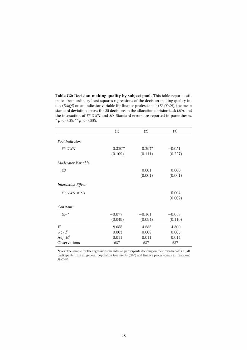
Table G2: Decision-making quality by subject pool. This table reports esti-mates from ordinary least squares regressions of the decision-making quality in-dex (DMQI ) on an indicator variable for �nance professionals (FP-OWN ), the meanstandard deviation across the 25 decisions in the allocation decision task (SD), andthe interaction of FP-OWN and SD. Standard errors are reported in parentheses.* p < 0.05, ** p < 0.005.

(1) (2) (3)

Pool Indicator:

FP-OWN 0.320** 0.297* ≠0.051(0.109) (0.111) (0.227)

Moderator Variable:

SD 0.001 0.000(0.001) (0.001)

Interaction E�ect:

FP-OWN ◊ SD 0.004(0.002)

Constant:

GP-* ≠0.077 ≠0.161 ≠0.058(0.049) (0.094) (0.110)

F 8.655 4.885 4.300p > F 0.003 0.008 0.005Adj. R2 0.011 0.011 0.014Observations 687 687 687

Notes: The sample for the regressions includes all participants deciding on their own behalf, i.e., allparticipants from all general population treatments (GP-*) and �nance professionals in treatmentFP-OWN .

28

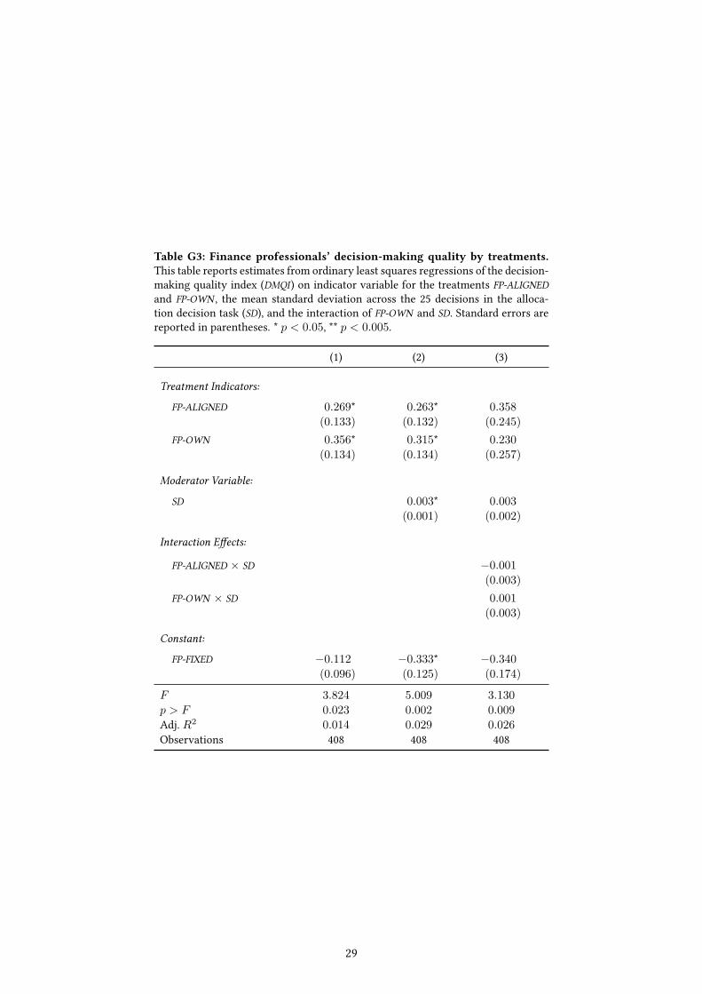
Table G3: Finance professionals’ decision-making quality by treatments.This table reports estimates from ordinary least squares regressions of the decision-making quality index (DMQI ) on indicator variable for the treatments FP-ALIGNEDand FP-OWN , the mean standard deviation across the 25 decisions in the alloca-tion decision task (SD), and the interaction of FP-OWN and SD. Standard errors arereported in parentheses. * p < 0.05, ** p < 0.005.

(1) (2) (3)

Treatment Indicators:

FP-ALIGNED 0.269* 0.263* 0.358(0.133) (0.132) (0.245)

FP-OWN 0.356* 0.315* 0.230(0.134) (0.134) (0.257)

Moderator Variable:

SD 0.003* 0.003(0.001) (0.002)

Interaction E�ects:

FP-ALIGNED ◊ SD ≠0.001(0.003)

FP-OWN ◊ SD 0.001(0.003)

Constant:

FP-FIXED ≠0.112 ≠0.333* ≠0.340(0.096) (0.125) (0.174)

F 3.824 5.009 3.130p > F 0.023 0.002 0.009Adj. R2 0.014 0.029 0.026Observations 408 408 408

29

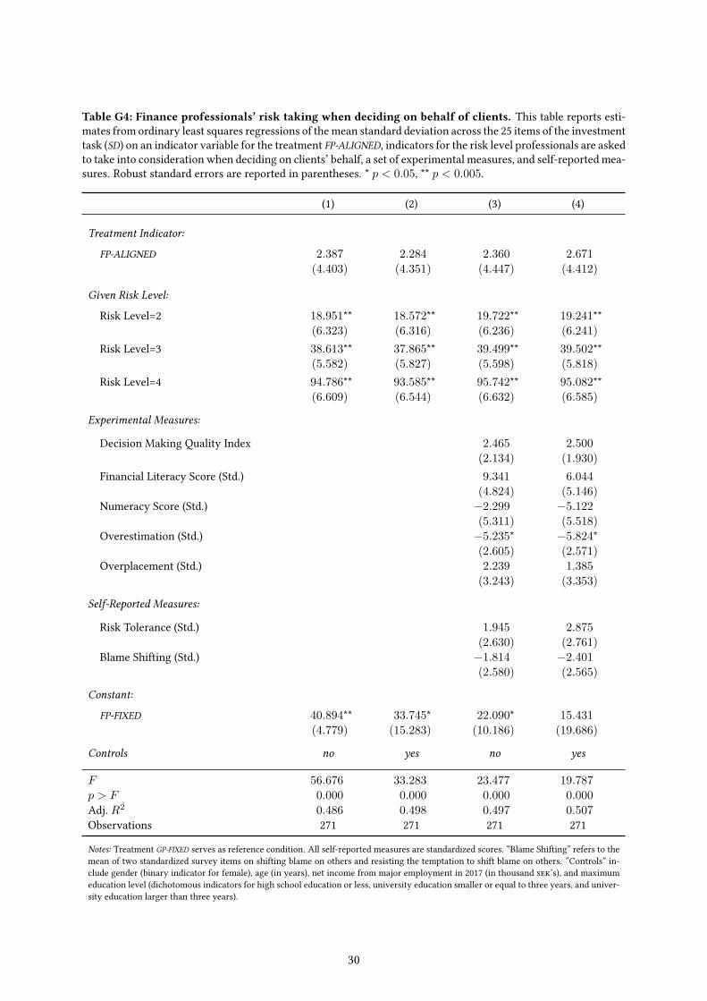
Table G4: Finance professionals’ risk taking when deciding on behalf of clients. This table reports esti-mates from ordinary least squares regressions of themean standard deviation across the 25 items of the investmenttask (SD) on an indicator variable for the treatment FP-ALIGNED, indicators for the risk level professionals are askedto take into consideration when deciding on clients’ behalf, a set of experimental measures, and self-reported mea-sures. Robust standard errors are reported in parentheses. * p < 0.05, ** p < 0.005.

(1) (2) (3) (4)

Treatment Indicator:

FP-ALIGNED 2.387 2.284 2.360 2.671(4.403) (4.351) (4.447) (4.412)

Given Risk Level:

Risk Level=2 18.951** 18.572** 19.722** 19.241**(6.323) (6.316) (6.236) (6.241)

Risk Level=3 38.613** 37.865** 39.499** 39.502**(5.582) (5.827) (5.598) (5.818)

Risk Level=4 94.786** 93.585** 95.742** 95.082**(6.609) (6.544) (6.632) (6.585)

Experimental Measures:

Decision Making Quality Index 2.465 2.500(2.134) (1.930)

Financial Literacy Score (Std.) 9.341 6.044(4.824) (5.146)

Numeracy Score (Std.) ≠2.299 ≠5.122(5.311) (5.518)

Overestimation (Std.) ≠5.235* ≠5.824*(2.605) (2.571)

Overplacement (Std.) 2.239 1.385(3.243) (3.353)

Self-Reported Measures:

Risk Tolerance (Std.) 1.945 2.875(2.630) (2.761)

Blame Shifting (Std.) ≠1.814 ≠2.401(2.580) (2.565)

Constant:

FP-FIXED 40.894** 33.745* 22.090* 15.431(4.779) (15.283) (10.186) (19.686)

Controls no yes no yes

F 56.676 33.283 23.477 19.787p > F 0.000 0.000 0.000 0.000Adj. R2 0.486 0.498 0.497 0.507Observations 271 271 271 271

Notes: Treatment GP-FIXED serves as reference condition. All self-reported measures are standardized scores. “Blame Shifting” refers to themean of two standardized survey items on shifting blame on others and resisting the temptation to shift blame on others. “Controls” in-clude gender (binary indicator for female), age (in years), net income from major employment in 2017 (in thousand ���’s), and maximumeducation level (dichotomous indicators for high school education or less, university education smaller or equal to three years, and univer-sity education larger than three years).

30

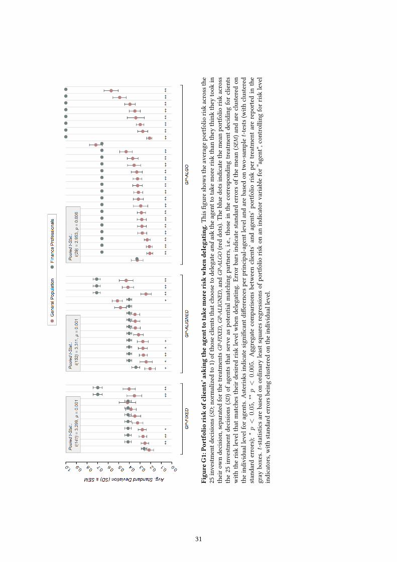
Figu

reG1:Po

rtfolio

risk

ofclients’asking

theag

enttotake

morerisk

whe

nde

lega

ting

.This�

gure

show

sthe

averagepo

rtfolio

riskacrossthe

25investmentd

ecisions

(SD;n

ormalized

to1)

ofthoseclientsthatcho

oseto

delegate

andasktheagenttotake

moreris

kthan

they

thinkthey

took

intheiro

wndecision

,separated

forthe

treatm

ents

GP-FIXE

D,G

P-ALIGNED

,and

GP-ALG

O(red

dots).Th

eblue

dotsindicate

themeanpo

rtfolio

riskacross

the25

investmentd

ecisions

(SD)o

fagentsthat

serveas

potentialm

atchingpartners,i.e.,thosein

thecorrespo

ndingtreatm

entd

ecidingforclients

with

theris

klevelthatm

atches

theirdesiredris

klevelw

hendelegatin

g.Errorbars

indicate

standard

errors

ofthemean(SEM

)and

areclusteredon

theindividu

allevelfor

agents.A

sterisks

indicate

sign

i�cant

di�e

rences

perp

rincipal-a

gent

leveland

arebasedon

two-sample

t-tests(w

ithclustered

standard

errors);*

p<

0.05,**

p<

0.00

5.Aggregate

comparis

onsbetw

eenclients’

andagents’p

ortfo

lioris

kpertreatm

entarerepo

rted

inthe

gray

boxes.

t-statistic

sarebasedon

ordinary

leastsqu

ares

regression

sof

portfolio

riskon

anindicatorvaria

blefor“

agent”,

controlling

forr

isklevel

indicators,w

ithstandard

errors

beingclusteredon

theindividu

allevel.

31

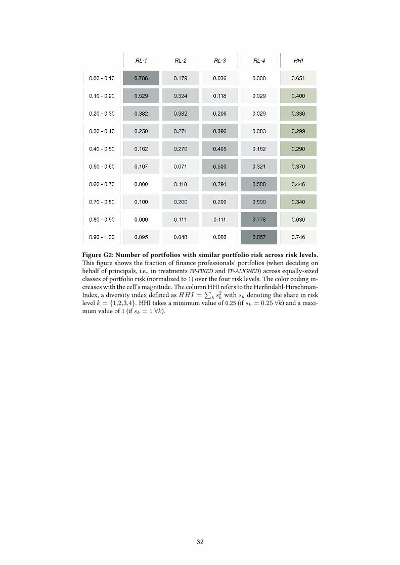
Figure G2: Number of portfolios with similar portfolio risk across risk levels.This �gure shows the fraction of �nance professionals’ portfolios (when deciding onbehalf of principals, i.e., in treatments FP-FIXED and FP-ALIGNED) across equally-sizedclasses of portfolio risk (normalized to 1) over the four risk levels. The color coding in-creases with the cell’s magnitude. The columnHHI refers to theHer�ndahl-Hirschman-Index, a diversity index de�ned as HHI =

qk s

2k with sk denoting the share in risk

level k = {1,2,3,4}. HHI takes a minimum value of 0.25 (if sk = 0.25 ’k) and a maxi-mum value of 1 (if sk = 1 ’k).

32

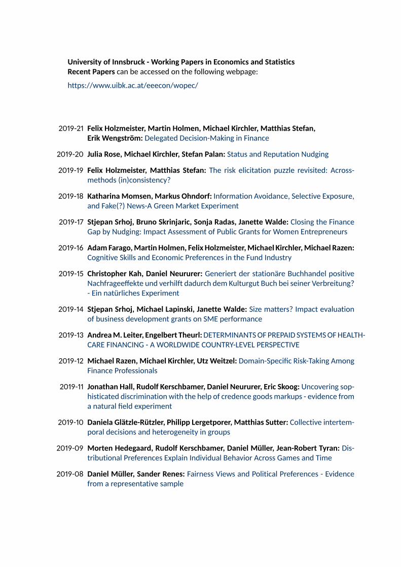
University of Innsbruck - Working Papers in Economics and StatisticsRecent Papers can be accessed on the following webpage:

https://www.uibk.ac.at/eeecon/wopec/

����-�� Felix Holzmeister, Martin Holmen, Michael Kirchler, Matthias Stefan,Erik Wengström: Delegated Decision-Making in Finance

����-�� Julia Rose, Michael Kirchler, Stefan Palan: Status and Reputation Nudging

����-�� Felix Holzmeister, Matthias Stefan: The risk elicitation puzzle revisited: Across-methods (in)consistency?

����-�� Katharina Momsen, Markus Ohndorf: Information Avoidance, Selective Exposure,and Fake(?) News-A Green Market Experiment

����-�� Stjepan Srhoj, Bruno Skrinjaric, Sonja Radas, Janette Walde: Closing the FinanceGap by Nudging: Impact Assessment of Public Grants for Women Entrepreneurs

����-�� AdamFarago,Martin Holmen, Felix Holzmeister,Michael Kirchler,Michael Razen:Cognitive Skills and Economic Preferences in the Fund Industry

����-�� Christopher Kah, Daniel Neururer: Generiert der stationäre Buchhandel positiveNachfragee�ekte und verhilft dadurch dem Kulturgut Buch bei seiner Verbreitung?- Ein natürliches Experiment

����-�� Stjepan Srhoj, Michael Lapinski, Janette Walde: Size matters? Impact evaluationof business development grants on SME performance

����-�� AndreaM. Leiter, Engelbert Theurl:DETERMINANTSOFPREPAID SYSTEMSOFHEALTH-CARE FINANCING - A WORLDWIDE COUNTRY-LEVEL PERSPECTIVE

����-�� Michael Razen, Michael Kirchler, Utz Weitzel: Domain-Speci�c Risk-Taking AmongFinance Professionals

����-�� Jonathan Hall, Rudolf Kerschbamer, Daniel Neururer, Eric Skoog: Uncovering sop-histicated discrimination with the help of credence goodsmarkups - evidence froma natural �eld experiment

����-�� Daniela Glätzle-Rützler, Philipp Lergetporer, Matthias Sutter: Collective intertem-poral decisions and heterogeneity in groups

����-�� Morten Hedegaard, Rudolf Kerschbamer, Daniel Müller, Jean-Robert Tyran: Dis-tributional Preferences Explain Individual Behavior Across Games and Time

����-�� Daniel Müller, Sander Renes: Fairness Views and Political Preferences - Evidencefrom a representative sample

����-�� Florian Lindner, Michael Kirchler, Stephanie Rosenkranz, Utze Weitzel: Social Sta-tus and Risk-Taking in Investment Decisions

����-�� Christoph Huber, Julia Rose: Individual attitudes andmarket dynamics towards im-precision

����-�� Felix Holzmeister, Jürgen Huber, Michael Kirchler, Florian Lindner, Utz Weitzel,Stefan Zeisberger: What Drives Risk Perception? A Global Survey with FinancialProfessionals and Lay People

����-�� David M. McEvoy, Tobias Haller, Esther Blanco: The Role of Non-Binding Pledgesin Social Dilemmas with Mitigation and Adaptation

����-�� KatharinaMomsen,MarkusOhndorf:Whendopeople exploitmoralwiggle room?An experimental analysis in a market setup

����-�� Rudolf Kerschbamer, Daniel Neururer, Matthias Sutter: Credence goods marketsand the informational value of new media: A natural �eld experiment

����-�� Martin Geiger, Eric Mayer, Johann Scharler: Inequality and the Business Cycle: Evi-dence from U.S. survey data

����-�� Matthias Sutter, Jürgen Huber, Michael Kirchler, Matthias Stefan, Markus Walzl:Where to look for the morals in markets?

����-�� Rene Schwaiger, Michael Kirchler, Florian Lindner, Utz Weitzel: Determinants ofinvestor expectations and satisfaction. A study with �nancial professionals

����-�� Andreas Groll, Julien Hambuckers, Thomas Kneib, Nikolaus Umlauf: LASSO-TypePenalization in the Framework of Generalized Additive Models for Location, Scaleand Shape

����-�� Christoph Huber, Jürgen Huber: Scale matters: Risk perception, return expecta-tions, and investment propensity under di�erent scalings

����-�� Thorsten Simon, Georg J. Mayr, Nikolaus Umlauf, Achim Zeileis: Lightning predic-tion using model output statistics

����-�� Martin Geiger, Johann Scharler: How do consumers interpret the macroeconomice�ects of oil price �uctuations? Evidence from U.S. survey data

����-�� Martin Geiger, Johann Scharler: How do people interpret macroeconomic shocks?Evidence from U.S. survey data

����-�� Sebastian J. Dietz, Philipp Kneringer, Georg J. Mayr, Achim Zeileis: Low visibilityforecasts for di�erent �ight planning horizons using tree-based boosting models

����-�� Michael Pfa�ermayr: Trade creation and trade diversion of regional trade agree-ments revisited: A constrained panel pseudo-maximum likelihood approach

����-�� Achim Zeileis, Christoph Leitner, Kurt Hornik: Probabilistic forecasts for the ����FIFA World Cup based on the bookmaker consensus model

����-�� Lisa Schlosser, TorstenHothorn, Reto Stau�er, Achim Zeileis:Distributional regres-sion forests for probabilistic precipitation forecasting in complex terrain

����-�� Michael Kirchler, Florian Lindner, Utz Weitzel: Delegated decision making and so-cial competition in the �nance industry

����-�� Manuel Gebetsberger, Reto Stau�er, Georg J. Mayr, Achim Zeileis: Skewed logisticdistribution for statistical temperature post-processing in mountainous areas

����-�� Reto Stau�er, Georg J.Mayr, JakobW.Messner, Achim Zeileis:Hourly probabilisticsnow forecasts over complex terrain: A hybrid ensemble postprocessing approach

����-�� Utz Weitzel, Christoph Huber, Florian Lindner, Jürgen Huber, Julia Rose, MichaelKirchler: Bubbles and �nancial professionals

����-�� Carolin Strobl, Julia Kopf, Raphael Hartmann, Achim Zeileis: Anchor point selec-tion: An approach for anchoring without anchor items

����-�� Michael Greinecker, Christopher Kah: Pairwise stablematching in large economies

����-�� Max Breitenlechner, Johann Scharler: How does monetary policy in�uence banklending? Evidence from the market for banks’ wholesale funding

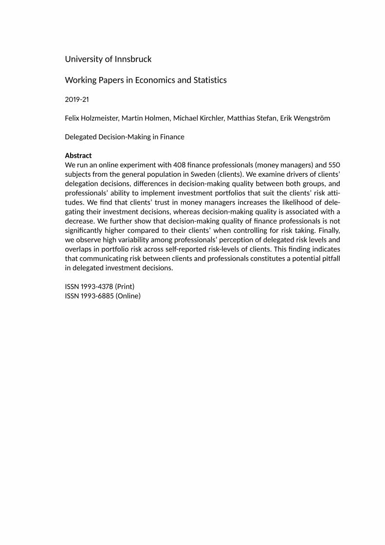
University of Innsbruck

Working Papers in Economics and Statistics

����-��

Felix Holzmeister, Martin Holmen, Michael Kirchler, Matthias Stefan, Erik Wengström

Delegated Decision-Making in Finance

AbstractWe run an online experiment with ��� �nance professionals (money managers) and ���subjects from the general population in Sweden (clients). We examine drivers of clients’delegation decisions, di�erences in decision-making quality between both groups, andprofessionals’ ability to implement investment portfolios that suit the clients’ risk atti-tudes. We �nd that clients’ trust in money managers increases the likelihood of dele-gating their investment decisions, whereas decision-making quality is associated with adecrease. We further show that decision-making quality of �nance professionals is notsigni�cantly higher compared to their clients’ when controlling for risk taking. Finally,we observe high variability among professionals’ perception of delegated risk levels andoverlaps in portfolio risk across self-reported risk-levels of clients. This �nding indicatesthat communicating risk between clients and professionals constitutes a potential pitfallin delegated investment decisions.

ISSN ����-���� (Print)ISSN ����-���� (Online)