Delay-dependent anti-windup synthesis for stability of constrained state delay systems using pole-constraints

ISA Transactions 50 (2011) 249–255

Contents lists available at ScienceDirect

ISA Transactions

journal homepage: www.elsevier.com/locate/isatrans

Delay-dependent anti-windup synthesis for stability of constrained state delaysystems using pole-constraintsAbrar Ahmed ∗, Muhammad Rehan, Naeem IqbalDepartment of Electrical Engineering, Pakistan Institute of Engineering and Applied Sciences (PIEAS), Islamabad, Pakistan

a r t i c l e i n f o

Article history:Received 15 July 2010Received in revised form24 October 2010Accepted 13 November 2010Available online 4 December 2010

Keywords:Anti-windup compensatorTime-delay systemsLinear matrix inequalities

a b s t r a c t

This paper proposes the design of anti-windup compensator gain for stability of actuator inputconstrained state delay systems using constrained pole-position of the closed-loop. Based on Delay-Dependent Lyapunov–Krasovskii functionals and local sector conditions, a new LMI characterization isderived that ensures closed-loop asymptotic stability of constrained state delay systemswhile accountingupper bound fixed state delay and largest lower bound of the system’s pole-position in the formulationof anti-windup gain. Besides, at saturation, the method significantly nullifies the inherent slow dynamicspresent in the system. It is shown in the comparative numerical examples that the LMI formulation drawsstability with improved time-domain performance.

© 2010 ISA. Published by Elsevier Ltd. All rights reserved.

1. Introduction

The domain of actuator constrained time-delay systems hasalways been a vocal issue in the community of control engineers.Since, the existence of time-delay in a linear system is a majorsource of performance degradation and instability, therefore thissubject is dealtwith prime concern [1]. In the literature for stabilityand performance, [2] has a broad focusing of various methodsof stability analysis including both frequency and time domainmethods. Besides some survey papers by [3,4] and a book [5]cover significant overviews on time-delay stability. It is possibleto extend the Lyapunov stability theory to time-delay systems.It was first realized by [6] that such a ‘‘Lyapunov functional’’should depend on the delayed states. As physical actuators cannotdeliver unlimited signals to the controlled plants, numerousmethods exist to cater the problem but the most accepted oneis the incorporation of anti-windup compensator (AWC) withthe existing controller. This approach designs the controller intwo parts, the first part addresses performance in the absenceof actuator saturation and the second part addresses stabilityand performance in the presence of actuator saturation. Thisapproach of controller design explicitly incorporates anti-windupcompensation that is activated subject to the actuator’s saturationconstraint. The closed-loop poles of controller and plantmust lie inthe left-half complex plane. Thus anti-windup compensator does

∗ Corresponding author. Tel.: +92 51 2207381x3408, Cell No.: +92 300 5530072.E-mail addresses: [email protected] (A. Ahmed),

[email protected] (M. Rehan), [email protected] (N. Iqbal).

0019-0578/$ – see front matter© 2010 ISA. Published by Elsevier Ltd. All rights reservdoi:10.1016/j.isatra.2010.11.003

not disturb the nominal linear controller’s design and becomesfunctional only in the saturation region ensuring closed-loopstability and resilience. Therefore, the literature [7–11] signi-ficantly highlights dynamic anti-windup compensator design andstability for actuator constrained time-delay systems. The studyfocused constrained linear single state delay systems. Further-ing this approach with new dimensions, the work of [12–15]treats the problem with a solution of enlarging the domain ofstability or basin of attraction of the overall closed-loop system.These papers use anti-windup compensator gain Ec as a freeparameter to enlarge the domain of stability. The techniques usedensure asymptotic stability of the system but do not addressthe inherent slow dynamics present in the system. This papertherefore addresses the method in the form of delay-dependentLyapunov–Krasovskii functionals based LMI for removing theinherent slow dynamics present in the actuator constrainedsystems besides ensuring asymptotic stability at upper fixedstate delay bound with anti-windup compensator gain. The slowdynamics are removed while applying constraints on the system’sclosed-loop pole-position. The method does not alter the originaldynamics of the plant. Instead the pole-position of the overallclosed-loop system is tapped. This procedure may also induce lag,if desired in the process. In the literature [16], such a constraintis defined as the decay rate or largest Lyapunov exponent orthe stability degree of the closed-loop system. It is primarily thenegative of the maximum real part of the eigenvalues of theclosed-loop system that ensures improved exponential stability.The constraint is fixed in the LMI resulting in anti-windup gain thatleads to the removal of slow dynamics. The resultant LMI is solvedusing a convex optimization technique. It is vocally said that theschemepresented in the paper also enlarges the domain of stability

ed.

http://dx.doi.org/10.1016/j.isatra.2010.11.003

http://www.elsevier.com/locate/isatrans

http://www.elsevier.com/locate/isatrans

mailto:[email protected]



http://dx.doi.org/10.1016/j.isatra.2010.11.003

250 A. Ahmed et al. / ISA Transactions 50 (2011) 249–255

in terms of ascertaining the upper state’s delay bound whileensuring stability. The work in this paper excels that of [17] byaddressing constrained state delay systems and finding an upperdelay bound besides removing slow dynamics in the formulationof anti-windup gain. The comparative numerical examples amplysignify the efficacy of the method.

2. Problem formulation

2.1. System description

Consider a linear plant with a state delay,

x(t) = Ax(t)+ Adx(t − τ)+ Bu(t)y(t) = Cx(t)

(1)

with initial condition function

x(t) = φ(t), t ∈ [−τ , 0] (2)

where x(t) ∈ ℜn is the state and τ is the unknown constant plant

state delay.Besides, u(t) ∈ ℜ

m and y(t) ∈ ℜm are the plant’s input

and measured output. We consider the input vector u to undergoamplitude constraint asu(i) ≤ u0(i), u0(i) > 0, i = 1, . . . ,m. (3)

We take the controller in a closed-loop with the plant

η(t) = Acη(t)+ Bcy(t)yc(t) = Ccη(t)+ Dcy(t)

(4)

where η(t) ∈ ℜnc is the controller’s state, uc(t) = y(t) ∈ ℜ

m is thecontroller’s input and yc(t) ∈ ℜ

m is the controller’s output. In thedefined feature, we take the dead zone signal as yc(t)− sat(yc(t))or yc(t) − u0(i), provided yc(t) > sat(yc(t)) or yc(t) > u0(i).The controller’s selection ensures stability and performance in theabsence of plant input constraint. Thus to overcome the brunt ofinstability at the time of saturation, the anti-windup compensatorgain Ec ∈ ℜ

nc×m is incorporated with the controller. Now thecontroller is modified with an anti-windup compensator as

η(t) = Acη(t)+ BcCx(t)+ Ec(sat(yc(t))− yc(t)) (5)yc(t) = Ccη(t)+ DcCx(t). (6)

Using (1) and (5), we define an extended state vector ξ(t) =

[x(t)T η(t)T ]T ∈ ℜn+nc or ℜ

nξ and the following matrices as

A =

[A + BDcC BCc

BcC Ac

], Ad =

[Ad 00 0

],

B =B 0nc×m

T, R =

0nc×n Inc

T,

K =DcC Cc

.

Now the closed-loop system reads

ξ (t) = Aξ(t)+ Adξ(t − τ)− (B + REc)ψ(Kξ(t)). (7)

Matrix A, not necessarily, is Hurwitz for delay-dependent analysis.Deriving coefficient orders in the closed-loop state model givesA ∈ ℜ

nξ×nξ ,Ad ∈ ℜnξ×nξ ,B ∈ ℜ

nξ×m,R ∈ ℜnξ×nc , Ec ∈ ℜ

nc×m

and K ∈ ℜm×nξ . Here ψ(Kξ(t)) = yc(t) − sat(yc(t)) = Kξ(t) −

sat(Kξ(t)) is the dead zone nonlinear signal as defined earlier.The augmented initial condition functions of (7) are defined to

be

ξ(t0 + θ) = φξ (θ) =

[x(t0 + θ)η(t0 + θ)

]=

[φx(θ)φη(θ)

],

∀θ ∈−τ , 0

;

where φξ (θ) satisfies ‖φξ‖c ≤ v, v > 0.

Using the Leibnitz–Newton formula andModel Transformation,we get

ξ (t) = (A + Ad)ξ(t)− (B + REc)ψ(Kξ(t))

− Ad

∫ 0

−τ

Aξ(t + θ)dθ

+ Ad

∫ 0

−τ

(B + REc)ψ(Kξ(t + θ))dθ

−

∫ 0

−τ

AdAdξ(t + θ − τ)dθ. (8)

Stability of (8) implies the stability of the original system (7).However, the reverse is not necessarily true because of thepresence of additional dynamics [1]. System (7) is globally asymp-totically stable if for any initial condition satisfying the statednorm condition of φξ (θ), the system’s state trajectories convergeasymptotically to the origin [14].

The problem would be to find the AWC’s gain Ec , upper bound onstate delay and largest lower bound on the pole-position of the closed-loop system.

3. AWC and stability of state delay systems

3.1. Delay-dependent analysis

Taking the Lyapunov–Krasovskii (LK) functional candidate as

V (ξ(t)) = V1(ξt)+ V2(ξt)+ V3(ξt) (9)

V1(ξt) = ξ(t)TPξ(t)+

∫ 0

−τ

∫ t

t+θψ(Kξ(Λ))T (B + REc)TH−1

× (B + REc)ψ(Kξ(Λ))dΛ

dθ (10)

V2(ξt) = −

∫ 0

−τ

∫ t

t+θξ(Λ)T S10ξ(Λ)dΛ

dθ (11)

V3(ξt) = −

∫−τ

−2τ

∫ t

t+θξ(Λ)T S11ξ(Λ)dΛ

dθ (12)

where P ∈ ℜnξ×nξ ,H ∈ ℜ

nξ×nξ , S10 ∈ ℜnξ×nξ , S11 ∈ ℜ

nξ×nξ aresymmetric positive-definite matrices.

Using (8) we have

V1(ξt) = ξ(t)T (ATP + PA + ATdP + PAd)ξ(t)

− 2Pξ(t)TAd

∫ 0

−τ

(Aξ(t + θ)+ Adξ(t + θ − τ))dθ

− 2Pξ(t)T (B + REc)ψ(Kξ(t))

+ 2Pξ(t)T∫ 0

−τ

Ad(B + REc)ψ(Kξ(t + θ))dθ

+ τψ(Kξ(t))T (B + REc)TH−1(B + REc)ψ(Kξ(t))

−

∫ 0

−τ

ψ(Kξ(t + θ))T (B + REc)T

×H−1(B + REc)ψ(Kξ(t + θ))dθ. (13)

Now, consider a matrix F ∈ ℜm×nξ , such that a constraint is

developed asK(i) − F(i) ξ ≤ u0(i), i = 1, . . . ,m (14)

leading to sector condition ψ(Kξ(t))TT [ψ(Kξ(t))− Fξ(t)] ≤ 0.Here T ∈ ℜ

m×m > 0, a diagonal matrix. Therefore, V1(ξt) is ex-tended to

V1(ξt) ≤ V1(ξt)− 2ψ(Kξ(t))TT [ψ(Kξ(t))− Fξ(t)] < 0. (15)

A. Ahmed et al. / ISA Transactions 50 (2011) 249–255 251

Solving the following term in V1(ξt) using the inequality 2uTv ≤

uTMu+vTM−1vwhereM is any symmetric positive definitematrixand u and v are vectors of appropriate dimensions.

− 2ξ(t)TP(B + REc)ψ(Kξ(t))− 2ψ(Kξ(t))TTψ(Kξ(t))+ 2ψ(Kξ(t))TTFξ(t)+ τψ(Kξ(t))T (B + REc)T

×H−1(B + REc)ψ(Kξ(t))≤ ξ(t)T (F TT − P(B + REc))T (2T − τ(B + REc)T

×H−1(B + REc))−1(F TT − P(B + REc))ξ(t). (16)

Replacing the inequality in V1(ξt)

V1(ξt) = ξ(t)T (ATP + PA + ATdP + PAd

+ (F TT − P(B + REc))T (2T − τ(B + REc)T

×H−1(B + REc))−1(F TT − P(B + REc)))ξ(t)

− 2Pξ(t)TAd

∫ 0

−τ

(Aξ(t + θ)+ Adξ(t + θ − τ))dθ

+ 2Pξ(t)T∫ 0

−τ


−

∫ 0

−τ


×H−1(B + REc)ψ(Kξ(t + θ))dθ. (17)

Solving the three integral terms in V1(ξt) separately

2ξ(t)TP∫ 0

−τ

AdAξ(t + θ)dθ ≤ τξ(t)TPAdAS−110 ATAT

dPξ(t)

+

∫ 0

−τ

ξ(t + θ)T S10ξ(t + θ)dθ (18)

2ξ(t)TP∫ 0

−τ

AdAdξ(t + θ − τ)dθ ≤ τξ(t)TPAdAdS−111 AT

dATdPξ(t)

+

∫ 0

−τ

ξ(t + θ − τ)T S11ξ(t + θ − τ)dθ (19)

2ξ(t)TP∫ 0

−τ


≤ τξ(t)TPAdHATdPξ(t)+

∫ 0

−τ


×H−1(B + REc)ψ(Kξ(t + θ))dθ. (20)

Finally V1(ξt) becomes, after replacing the integral terms

V1(ξt) = ξ(t)T (ATP + PA + ATdP + PAd


×H−1(B + REc))−1(F TT − P(B + REc)))ξ(t)− τξ(t)TPAdAS−1

10 ATATdPξ(t)

−

∫ 0

−τ

ξ(t + θ − τ)T S11ξ(t + θ − τ)dθ

− τξ(t)TPAdAdS−111 AT

dATdPξ(t)+ τξ(t)TPAdHAT

dPξ(t)

−

∫ 0

−τ

ξ(t + θ)T S10ξ(t + θ)dθ. (21)

Taking the remaining derivatives of (11) and (12)

V2(ξt) = −τξ(t)T S10ξ(t)+

∫ 0

−τ

ξ(t + θ)T S10ξ(t + θ)dθ (22)

V3(ξt) = −τξ(t)T S11ξ(t)

+

∫ 0

−τ

ξ(t + θ − τ)T S11ξ(t + θ − τ)dθ. (23)

Having summed (21)–(23) we get

V (ξ) ≤ ξ(t)T (ATP + PA + ATdP + PAd


×H−1(B + REc))−1(F TT − P(B + REc))− τPAdAS−1

10 ATATdP − τS11 − τPAdAdS−1

11 ATdAT

dP

+ τPAdHATdP − τS10)ξ(t) < 0. (24)

For stability using the constraint pole-position [16], we assumeV (ξ(t)) ≤ −2αξ(t)TPξ(t) for all trajectories. Then V (ξ(t)) ≤

V (ξ(0))e−2αt so that ‖ξ(t)‖ ≤ e−αtκ(P)1/2‖ξ(0)‖ for all trajecto-ries, and therefore, the decay rate or largest Lyapunov exponent orclosed-loop pole-position of (7) are at leastα. Stability correspondsto a positive decay rate.

Therefore (24) becomes,

V (ξ(t)) ≤ ξ(t)T (ATP + PA + ATdP + PAd + 2αP


×H−1(B + REc))−1(F TT − P(B + REc))− τPAdAS−1

10 ATATdP − τS11 − τPAdAdS−1

11 ATdAT

dP

+ τPAdHATdP − τS10)ξ(t) < 0. (25)

Rewriting (25) in LMI formΛ(P) (F T T − P(B + REc)) 0 τPAdA τPAdAd

∗ −2T τ(B + REc) 0 0∗ ∗ −τH 0 0∗ ∗ ∗ τS10 0∗ ∗ ∗ ∗ τS11

< 0 (26)

where Λ(P) = ATP + PA + PAd + ATdP + 2αP + τPAdHAT

dP −

τS10 − τS11.Pre- and post-multiplying (26) byW 0 0 0 00 G 0 0 00 0 Inξ 0 00 0 0 W 00 0 0 0 W

∈ ℜ(4nξ+m)×(4nξ+m) (27)

where G = T−1,G ∈ ℜm×m,W = P−1,W ∈ ℜ

nξ×nξ .This process of multiplication is called ‘‘Congruence Transfor-

mation’’. It is very useful for removing bilinear terms in matrixinequalities, in conjunction with a change of variables to make abilinear matrix inequality linear.

Making congruence transformation turns (26) toΛ(W ) (Y T

− BG − RZ) 0 τWAdA τWAdAd

∗ −2G τ(GBT+ ZTRT ) 0 0

∗ ∗ −τH 0 0∗ ∗ ∗ τΠ10 0∗ ∗ ∗ ∗ τΠ11

< 0 (28)

whereΛ(W ) = ATW +WA +WAd + ATdW + 2αW + τAdHAT

d −

τΠ10 − τΠ11,Π10 = WS10W ,Π11 = WS11W ,G = T−1,G ∈

ℜm×m, Y T

= WF T , Y ∈ ℜm×nξ , Z = EcG, Z ∈ ℜ

nc×m,W = P−1,W ∈ ℜ

nξ×nξ .LMI (28) ensures asymptotic stability of (7). Thus the anti-

windup gain Ec is calculated by fixing upper bound of state delayτ and largest lower bound of pole-position or decay rate α in (28).The two parameters fixed in the LMI may be taken from a givenset by which we may verify whether the asymptotic stability ofthe considered delay system class is guaranteed, this makes thestability problem a feasibility one.


LMI (28), if redefined with K = F turns toΛ(W ) (WKT

− BG − RZ) 0 τWAdA τWAdAd

∗ −2G τ(GBT+ ZT RT ) 0 0

∗ ∗ −τH 0 0∗ ∗ ∗ τΠ10 0∗ ∗ ∗ ∗ τΠ11

< 0. (29)

Thus LMI (29) ensures the global uniform asymptotic stabilityof (7).

3.2. Sector-constraint on controller

Regarding the sector-constraint on the controller, we assumeu20(i)

P ≥ (K − F)T (K − F), i = 1, . . . ,m.

This may be rewritten as[P KT

− F T

K − F u20(i)

]≥ 0, i = 1, . . . ,m. (30)

Pre- and post-multiplying (30) byW 00 I

,we finally get the sector-

constraint LMI[W WKT

− Y T

KW − Y u20(i)

]≥ 0, i = 1, . . . ,m. (31)

Thus the exponential and asymptotic stability of (7) is defined byLMIs (28) and (31).

4. Comparative analysis

The comparative analysis is based on finding the distinct timedomain behavior in state convergence of (7) using varied values ofpole-position or decay rate α and upper state delay bound τ .

Example 1. We take the plant and controller as in [12,15],

Ap =

[1 1.50.3 −2

], Apd =

[0 −10 0

],

Bp =

[101

], Cp =

5 1

Ac =

[−20.2042 2.52162.1415 −4.4821

], Bc =

[1.9516

−0.0649

],

Cc =−0.9165 0.1091

, Dc = 0.

The saturation is taken at u0 = 1, state delay bound τ ≤ 1 sand decay rate or largest lower bound α ≥ 100. The anti-windupgain Ec is calculated using LMIs (28) and (31). It is calculated tobe Ec =

−20.4450 −59.7402

. The value of α is drawn from

a pre-defined set of values in which the best possible asymptoticconvergence is obtained. Even defining the upper bound of τ ,would eventually ensure the feasible solution obtained from theLMIs. The value of u0 is taken small instead of 15 as in [12,15]to ascertain the marked effect of saturation. Initial conditions aretaken as

10 10 5 50

. Fig. 1 shows the state behavior.

By simulations it is found that at α = 100, the system startsconverging at reasonably optimal range. It is also implied that thedesigner has to select a value from this range either above or belowdepending on convergence rate. The above range of α than 100always produces optimal convergence rate. But the lower rangewould exponentially deteriorate the convergence and eventuallyexplode the system. We therefore study the deterioration inthe system state behavior at the lower range in the followingdescription.

We take u0 = 1, 97 ≤ α < 100, τ ≤ 1. Solving LMIs, givesEc =

5.8919 −63.5251


Fig. 1. System state trajectories at decay rate/state delay of α = 100, τ = 1.


Fig. 3. System state trajectories at decay rate/state delay of α = 95.5, τ = 1.


Since the largest lower bound is already ascertained, in Fig. 2the system convergence rate at α = 97 is derived. Controller stateis found un-damped. The plant converges appropriately.

Next we take u0 = 1, 95.5 ≤ α < 97, τ ≤ 1. Solving LMIs,gives Ec =

14.8236 −64.3366


In Fig. 3, the controller is seen further un-damped. Though, theplant’s convergence remains unchanged.

Next we take u0 = 1, 95 ≤ α < 95.5, τ ≤ 1. Solving LMIs,gives Ec =

18.1376 −64.0899


In Fig. 4, the controller is found to be oscillating and anticipatinga nonlinear effect to arise in the closed-loop system.

Next we take u0 = 1, α < 95, τ ≤ 1. Solving LMIs, givesEc =

20.1214 −63.9228


In Fig. 5, the system state is found to be exploding. It isattributed to the lower range value of α. A critical value of α maytherefore be selected to ensure the desired convergence.

Next we take u0 = 1, α ≥ 100, τ ≤ 2.5. Solving LMIs, givesEc =

3.1100 −0.2990



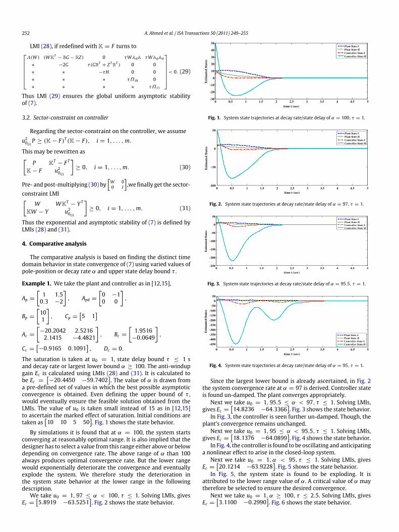
Fig. 5. System state trajectories at decay rate/state delay of α = 94.7, τ = 1.

Fig. 6. System state trajectories at decay rate/state delay of α = 100, τ = 2.5.

Fig. 7. System state trajectories of [15] without decay rate at state delay of τ = 1.

To further entrench the validity of LMIs (28) and (31), an upperdelay bound is selected. It is proved in Fig. 6 that the systemensures exponential and asymptotic stability. Our results excel [12,15] by proving an upper delay bound of 2.5 s than 1 s.

Now we infer, that the original system defined in [12,15]produces its state trajectories at the same initial condition as takenin the afore-stated discussion with u0 = 1 and τ = 1 as shownin Fig. 7. The delay-dependent anti-windup gain turns out to beEc =

5.3421 −6.2815

after having solved the LMIs defined

in [15]. The LMIs and state behavior do not take the pole-positionconstraint α into account.

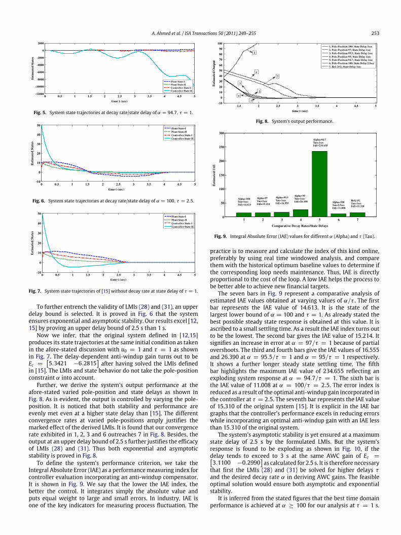
Further, we derive the system’s output performance at theafore-stated varied pole-position and state delays as shown inFig. 8. As is evident, the output is controlled by varying the pole-position. It is noticed that both stability and performance areevenly met even at a higher state delay than [15]. The differentconvergence rates at varied pole-positions amply justifies themarked effect of the derived LMIs. It is found that our convergencerate exhibited in 1, 2, 3 and 6 outreaches 7 in Fig. 8. Besides, theoutput at an upper delay bound of 2.5 s further justifies the efficacyof LMIs (28) and (31). Thus both exponential and asymptoticstability is proved in Fig. 8.

To define the system’s performance criterion, we take theIntegral Absolute Error (IAE) as a performancemeasuring index forcontroller evaluation incorporating an anti-windup compensator.It is shown in Fig. 9. We say that the lower the IAE index, thebetter the control. It integrates simply the absolute value andputs equal weight to large and small errors. In industry, IAE isone of the key indicators for measuring process fluctuation. The

Fig. 8. System’s output performance.

Fig. 9. Integral Absolute Error (IAE) values for different α (Alpha) and τ (Tau).

practice is to measure and calculate the index of this kind online,preferably by using real time windowed analysis, and comparethem with the historical optimum baseline values to determine ifthe corresponding loop needs maintenance. Thus, IAE is directlyproportional to the cost of the loop. A low IAE helps the process tobe better able to achieve new financial targets.

The seven bars in Fig. 9 represent a comparative analysis ofestimated IAE values obtained at varying values of α/τ . The firstbar represents the IAE value of 14.613. It is the state of thelargest lower bound of α = 100 and τ = 1. As already stated thebest possible steady state response is obtained at this value. It isascribed to a small settling time. As a result the IAE index turns outto be the lowest. The second bar gives the IAE value of 15.214. Itsignifies an increase in error at α = 97/τ = 1 because of partialovershoots. The third and fourth bars give the IAE values of 16.555and 26.390 at α = 95.5/τ = 1 and α = 95/τ = 1 respectively.It shows a further longer steady state settling time. The fifthbar highlights the maximum IAE value of 234.655 reflecting anexploding system response at α = 94.7/τ = 1. The sixth bar isthe IAE value of 11.008 at α = 100/τ = 2.5. The error index isreduced as a result of the optimal anti-windup gain incorporated inthe controller at τ = 2.5. The seventh bar represents the IAE valueof 15.310 of the original system [15]. It is explicit in the IAE bargraphs that the controller’s performance excels in reducing errorswhile incorporating an optimal anti-windup gain with an IAE lessthan 15.310 of the original system.

The system’s asymptotic stability is yet ensured at a maximumstate delay of 2.5 s by the formulated LMIs. But the system’sresponse is found to be exploding as shown in Fig. 10, if thedelay tends to exceed to 3 s at the same AWC gain of Ec =3.1100 −0.2990

as calculated for 2.5 s. It is therefore necessary

that first the LMIs (28) and (31) be solved for higher delays τand the desired decay rate α in deriving AWC gains. The feasibleoptimal solution would ensure both asymptotic and exponentialstability.

It is inferred from the stated figures that the best time domainperformance is achieved at α ≥ 100 for our analysis at τ = 1 s.


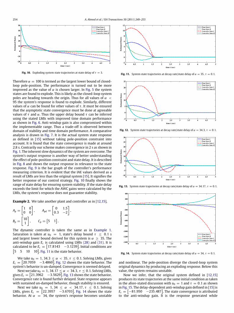
Fig. 10. Exploding system state trajectories at state delay of τ = 3.

Therefore α = 100 is termed as the largest lower bound of closed-loop pole-position. The performance is turned out to be moreimproved as the value of α is chosen larger. In Fig. 5 the systemstates are found to explode. This is likely as the closed-loop systempoles are heading towards the origin. Thus for all values of α <95 the system’s response is found to explode. Similarly, differentvalues of α can be found for other values of τ . It must be ensuredthat the asymptotic state convergence must be done at agreeablevalues of τ and α. Thus the upper delay bound τ can be inferredusing the stated LMIs with improved time domain performanceas shown in Fig. 6. Anti-windup gain is also compromised withinthe implementable range. Thus a trade-off is observed betweendomain of stability and time domain performance. A comparativeanalysis is drawn in Fig. 7. It is the actual system state responseas defined in [15] without taking pole-position constraint intoaccount. It is found that the state convergence is made at around2.8 s. Contrarily our scheme makes convergence in 2 s as shown inFig. 1. The inherent slowdynamics of the system are overcome. Thesystem’s output response is another way of better understandingthe effect of pole-position constraint and state delay. It is describedin Fig. 8 and shows the output response in relevance to the stateresponse. Fig. 9 is the bar graph of the controller’s performancemeasuring criterion. It is evident that the IAE values derived as aresult of LMIs are less than the original system [15]. It signifies thebetter response of our control strategy. Fig. 10 finally shows therange of state delay for ensuring system stability. If the state delayexceeds the limit for which the AWC gains were calculated by theLMIs, the system’s response does not guarantee stability.

Example 2. We take another plant and controller as in [12,15],

Ap =

[1 00 0

], Apd =

[0 1.50.3 −2

],

Bp =

[101

], Cp =

5 1

.

The dynamic controller is taken the same as in Example 1.Saturation is taken at u0 = 1, state’s delay bound τ ≤ 0.1 sand largest lower bound derived for this system is α ≥ 35. Theanti-windup gain Ec is calculated using LMIs (28) and (31). It iscalculated to be Ec =

17.8143 −3.1239

. Initial conditions are

5 5 10 10. Fig. 11 is the state behavior.

We take u0 = 1, 34.3 ≤ α < 35, τ ≤ 0.1. Solving LMIs, givesEc =

20.7059 −3.4860

. Fig. 12 shows the state behavior. The

system’s behavior is un-damped. Convergence is seemed delayed.Nextwe take u0 = 1, 34.17 ≤ α < 34.3, τ ≤ 0.1. Solving LMIs,

gives Ec =21.3962 −3.5629


Convergence rate is found further delayed. State response appearswith sustained un-damped behavior, though stability is ensured.

Next we take u0 = 1, 34 ≤ α < 34.17, τ ≤ 0.1. SolvingLMIs, gives Ec =

22.3957 −3.6703

. Fig. 14 shows the state

behavior. At α = 34, the system’s response becomes unstable


Fig. 12. System state trajectories at decay rate/state delay of α = 34.3, τ = 0.1.

Fig. 13. System state trajectories at decay rate/state delay of α = 34.17, τ = 0.1.


and nonlinear. The pole-position diverge the closed-loop systemoriginal dynamics by producing an exploding response. Below thisvalue, the system remains unstable.

Now we infer, that the original system defined in [12,15]produces its state trajectories at the same initial condition as takenin the afore-stated discussion with u0 = 1 and τ = 0.1 as shownin Fig. 15. The delay-dependent anti-windup gain defined in [15] isEc =

−81.950 −235.487

. The state convergence is attributed

to the anti-windup gain. It is the response generated while


Fig. 15. System state trajectories of [15] without decay rate at state delay ofτ = 0.1.

Fig. 16. System’s output performance.


only addressing the enlarged domain of stability and asymptoticconvergence in [15].

Further, we derive the system’s output performance at thevaried pole-position and state delays as shown in Fig. 16. Theoutput is controlled by varying the pole-position. The performanceagain clearly manifests the behavior of the system outputgenerated as a result of state response detailed above. It is evidenthow the pole-position affects the system’s output response byremoving the inherent slow dynamics by fast convergence asshown by 1, 2 and 7 in Fig. 16. Besides, the slow responses in4 and 6 may also be considered for adding an additional lagin the system. This may prove useful for inducing a lag in fastprocess variable controllers. Such a procedure may be adopted forreciprocating controller speed response at varying intervals. Theexploding response in 6 shows the unstable behavior of the system.

Lastly, we take u0 = 1, α ≥ 50, τ ≤ 1. Solving LMIs, gives Ec =4.9210 −0.5240

. Fig. 17 shows the state behavior. Again the

higher upper delay bound of 1 s than 0.4 s in [15] shows the effectof our LMIs. The convergence rate is also found fast. The aim ofthis paper is achieved after having resolved an upper delay boundand fast convergence besides ensuring asymptotic stability. TheFig. 17 again proves the objective. Though the system’s matrix A isunstable, the delay-dependent analysis proves the system stability

at upper delay bound. This adds to the enlargement of domain ofstability in terms of the state delay bounds of the plant.

The IAE of the controller at α = 35, τ = 0.1 is 4.418 and thatof [15] at τ = 0.1 is 9.140. It proves the better controller lawfollowed by the paper.

Having done a comparative inference, the work in [12,15]addresses only the enlargement of the domain of stabilityirrespective of the steady state time response and upper boundstate delay and [17] computes the dynamic anti-windup controllerwith pole-constraints for non-state delay systems.

Remarks. Examples are numerically solved using [18].

5. Conclusion

This paper exploited the effect of the largest Lyapunov exponentor the closed-loop pole-position on the stability of actuator-constrained state delay systems. The work is an extension tothe previous work in the literature in terms of addressingconstrained state delay systems and deriving the maximum delaybound with improved time domain performance. The methodeventually removes the inherent slow dynamics present in thesystem. Thus the implications of anti-windup compensator gainand constrained pole-position proved decisive in the improvedexponential stability of the closed-loop system.

References

[1] GuK,Niculescu S-I. Survey on recent results in the stability and control of time-delay systems. Journal of Dynamic Systems, Measurement and Control 2003;125:158–65.

[2] Kolmanovskii VB, Nosov VR. Stability of functional differential equations.Mathematics in science and eng, vol. 180. New York: Academic Press; 1986.

[3] Niculescu S-I, Verriest EI, Dugard L, Dion JM. Stability and robust stability oftime-delay systems: a guided tour. In: Dugards L, Verriest EI, editors. Stabilityand control of time-delay systems. LNCIS, vol. 228. 1997. p. 1–71.

[4] Kharitonov VL. Robust stability analysis of time-delay systems: a survey.Annual Reviews in Control 1999;23:185–96.

[5] Niculescu S-I. Delay effects on stability: a robust control approach. Heidelberg(Germany): Springer-Verlag; 2001.

[6] Krasovskii NN. Stability of motion, Moscow, 1959 [in Russian]. Englishtranslation: Stanford Uni. Press, 1963.

[7] Tarbouriech S, Turner M-C. Anti-windup design: an overview of some recentadvances and open problems. IET Control Theory and Applications 2009;3:1–19.

[8] Park J-K, Choi C-H, Choo H. Dynamic anti-windup method for a class of time-delay control systems with input saturation. International Journal of Robustand Nonlinear Control 2000;10:457–88.

[9] Zaccarian L, Nesic D, Teel AR. L2 anti-windup for linear dead-time systems.Systems & Control Letters 2005;54(12):1205–17.

[10] Tarbouriech S, Gomes Da Silva Jr JM. Synthesis of controllers for continuous-time delay systems with saturating controls via LMIs. IEEE Transactions onAutomatic Control 2000;45(1):105–11.

[11] Tarbouriech S, Gomes Da Silva Jr JM, Garcia G. Delay-dependent anti-windupstrategy for linear systems with saturating inputs and delayed outputs.International Journal of Robust and Nonlinear Control 2004;14:665–82.

[12] Qiang WY, Yan CY, Xian SY. Anti-windup compensator gain design for time-delay systems with constraints. Acta Automatica Sinica 2006;32(1).

[13] Tarbouriech S, Gomes Da Silva Jr JM, Garcia G. Delay-dependent anti-winduploops for enlarging the stability region of time-delay systems with saturatinginputs. ASME Journal of Dynamic Systems, Measurement, and Control 2003;125(1):265–7.

[14] Tarbouriech S, Queinnec I, Garcia G. Stability region enlargement throughanti-windup strategy for linear systems with dynamics restricted actuator.International Journal of Systems Science 2006;37(2):79–90.

[15] Gomes Da Silva Jr JM, Tarbouriech S, Garcia G. Using anti-windup loopsfor enlarging the stability region of time-delay systems subject to inputsaturation. In: Proceeding of the 2004 American control conference. 2004.p. 4819–24.

[16] Boyd S, Ghaoui LEl, Feron E, Balakrishnan V. Linear matrix inequalities insystem and control theory. In: SIAM studies in applied mathematics. vol. 15.Philadelphia (USA); 1994.

[17] Roos C, Biannic JM. A convex characterization of dynamically-constrained anti-windup controllers. Automatica 2008;44:2449–52.

[18] Grant M, Boyd S. CVX-toolbox. USA: Stanford Uni.; 2009.

Documents

Delay-dependent anti-windup synthesis for stability of constrained state delay systems using pole-constraints