Embed Size (px)
Citation preview

1
Delay Analysis of Wireless Federated Learning
Based on Saddle Point Approximation and
Large Deviation Theory
Lintao Li, Longwei Yang, Xin Guo, Member, IEEE, Yuanming Shi,
Senior Member, IEEE, Haiming Wang, Wei Chen, Senior Member, IEEE,
and Khaled B. Letaief, Fellow, IEEEAbstract
Federated learning (FL) is a collaborative machine learning paradigm, which enables deep learning
model training over a large volume of decentralized data residing in mobile devices without accessing
clients’ private data. Driven by the ever increasing demand for model training of mobile applica-
tions or devices, a vast majority of FL tasks are implemented over wireless fading channels. Due
to the time-varying nature of wireless channels, however, random delay occurs in both the uplink and
downlink transmissions of FL. How to analyze the overall time consumption of a wireless FL task,
or more specifically, a FL’s delay distribution, becomes a challenging but important open problem,
especially for delay-sensitive model training. In this paper, we present a unified framework to calculate
the approximate delay distributions of FL over arbitrary fading channels. Specifically, saddle point
approximation, extreme value theory (EVT), and large deviation theory (LDT) are jointly exploited to
find the approximate delay distribution along with its tail distribution, which characterizes the quality-
of-service of a wireless FL system. Simulation results will demonstrate that our approximation method
achieves a small approximation error, which vanishes with the increase of training accuracy.
Index Terms
Wireless federated learning, task-oriented communications, delay analysis, saddle point approxima-
tion, large deviation theory, extreme value theory.
This work is supported in part by the National Natural Science Foundation of China under Grant No. 61971264, the BeijingNatural Science Foundation under Grant No. 4191001, and Lenovo Research. The preliminary work has been accepted by IEEEICC 2021.
Lintao Li, Longwei Yang and Wei Chen are with the Department of Electronic Engineering, Tsinghua University, Beijing100084, China, and also with the Beijing National Reasearch Center for Information Science and Technology, TsinghuaUniversity, Beijing 100084, China (email: [email protected]; [email protected]; [email protected]).
Xin Guo and Haiming Wang are with Lenovo Research, Beijing 100094, China (email: [email protected];[email protected]).
Yuanming Shi is with the School of Information Science and Technology, ShanghaiTech University, Shanghai 201210, China(email: [email protected]).
Khaled B. Letaief is with the School of Engineering, Hong Kong University of Science and Technology, Clear Water Bay,Hong Kong, and also with Peng Cheng Laboratory, Shenzhen 518066, China (email: [email protected]).
arX
iv:2
103.
1699
4v2
[ee
ss.S
P] 1
Apr
202
1
2
I. INTRODUCTION
The phenomenal development of wireless networking and machine learning technologies
yields huge volume of sensory data at the wireless edge networks [1]. Meanwhile, as the
computational power and storage of mobile devices keep growing, mobile edge computing
(MEC) [2] is becoming a crucial technology for future networks to enable ultra-low power
and ultra-low latency applications at the edge [3]. By integrating federated learning (FL) and
edge computing with enhanced privacy and security guarantees, federated edge learning has
recently been receiving increasing attention to provide services and intelligence at the edge.
This is achieved by training machine learning models across a fleet of participating distributed
mobile devices without transferring their local private data to a remote centralized server at
either the edge or cloud. FL thus becomes a key technique to support the paradigm shift from
“connected things” to “connected intelligence” in 6G, where humans, things, and intelligence
are intertwined within a hyper-connected cyber-physical world [4], [5]. This inspires extremely
exciting 6G applications, including industrial Internet of Things (IIoT), Internet of Vehicles
(IoV), and healthcare [6]–[8]. However, the deployment of FL in wireless networks, poses
unique challenges in terms of system heterogeneity, statistical heterogeneity, and trustworthiness
[9], [10]. In particular, due to the fading nature and limited resources of wireless channels,
communication-efficiency becomes a key performance indicator to implement FL at scale in
wireless networks with low-latency, privacy and security guarantees.
To address the communication challenges in wireless FL, a growing body of recent works has
demonstrated the effectiveness of joint optimizing communication, computation and learning
across wireless networks. The analysis and design of wireless FL systems can be typically
divided into two categories: analog and digital communication protocols. Specifically, by ex-
ploiting the signal superposition property of a wireless multiple-access channel, analog FL has
recently received particular interest to implement low-latency global model aggregation (e.g., the
weighted average function computation) via over-the-air computation (AirComp). This scheme
can significantly reduce the communication bandwidth consumption and improve spectrum effi-
ciency via concurrent transmission of locally updated models. However, the channel noise in the
AirComp based model aggregation procedure yields a completely different type of distributed FL
algorithms with iterative noise. It turns out to be difficult to characterize the convergence rates,
complexity, optimality and statistical behaviors of the noisy FL algorithm iterates, for which
various communication-efficient analog distributed algorithms were developed with convergence
3
guarantees, e.g., analog gradient methods [11], quantization schemes [12], and gradient sparsifi-
cation approaches [13]. Moreover, resource allocation becomes critical to improve the learning
convergence rate and model prediction accuracy in wireless FL, including the transmission power
control [13]–[16], model aggregation beamforming [17], [18], and device scheduling [18]–[21].
However, analog wireless FL system normally requires a strict synchronization at the symbol
level and the aggregation procedure of the underlying distributed learning algorithms is inherently
corrupted by channel noise.
In contrast, digital wireless FL systems are able to leverage advanced coding schemes and
mobile edge computing techniques, thereby achieving channel noise robustness and low-latency
transmission during the distributed wireless FL procedure. Various communication network
architectures, e.g., single-server, hierarchical and decentralized wireless FL systems, have re-
cently been proposed to improve the communication efficiency and learning performance. In
particular, numerous research efforts have been made to minimize the training delay of single-
server FL systems, including device scheduling policies for mitigating the stragglers (i.e., the
training bottleneck caused by the slowest participating devices) [22]–[28], resource allocation for
improving the transmission efficiency [27]–[30], adaptive aggregation for dynamically controlling
the aggregation frequency [31] or calibrating aggregation weights [32], batchsize selection for
improving learning efficiency [33], and incentive mechanisms for reducing the side effects of
information asymmetry [34], [35]. To further address the heterogeneity in terms of computation
and communication capabilities across devices, hierarchical FL was advocated to orchestrate
nodes for cooperative learning [36]. To this end, a partial model aggregation approach was
proposed in [37] to cope with communication bottlenecks, while a collaborative FL was proposed
in [38] for enabling on-device learning with less reliance on a central server. Besides, to
improve the system robustness and alleviate the straggler effect, a decentralized device-to-device
communication enabled FL network architecture was proposed in [39], which is supported by
radio resource allocation and computation loads adjustment.
Although there have already been a number of published works related to the delay minimiza-
tion in both analog and digital transmission schemes, a delay distribution analysis has not yet
been carried out for wireless FL systems. Indeed, delay distribution is critical and has profound
implications for resource budgeting and timeout probability assessment under delay constraints.
In this paper, we shall propose a novel framework to characterize the delay distribution analysis
in wireless FL systems, for which we conceive a versatile saddle point approximation based
4
method. Specifically, we first characterize the distribution of one user’s uplink delay by the saddle
point approximation method. Based on the characteristics of the synchronous and asynchronous
downlink transmission schemes, the distributions of one iteration delay are further obtained
along with the distributions of the overall delay. Besides, extreme value theory (EVT) [40] and
large deviation theory (LDT) [41] are also exploited to reveal the asymptotic properties of the
delay distribution in wireless FL systems. To address the challenge in theoretically deriving
the accurate number of convergence rounds, we model the number of convergence rounds as a
random variable in lieu of a constant, followed by using an empirical distribution to investigate
the overall delay in the general wireless FL systems with nonconvex FL models.
The main contribution of this paper is the analysis of the distribution of the one iteration
and overall delay in wireless FL systems. To the best of our knowledge, this is the first work
that provides a theoretical analysis of the delay distribution in wireless FL systems. The major
contributions are summarized as follows:
• We establish a unified FL modeling framework over wireless fading channels to analyze
the distribution of training delay caused by wireless communication under the practical
condition that the transmission time is larger than the coherence time.
• A transmission model consisting of the uplink and downlink transmission is proposed, for
which both synchronous and asynchronous downlink transmission schemes are developed
for different application scenarios.
• To characterize the delay distribution in wireless FL systems, we propose a saddle point
approximation based method. Moreover, EVT and LDT are leveraged to reveal asymptotic
properties of the delay distribution in wireless FL systems.
• Extensive experiments demonstrate that the simulation results are in good agreement with the
established theoretical results. In particular, for one iteration delay, the theoretical results
perfectly match with the simulation results, which verifies the validity of the proposed
methods.
The rest of this paper is organized as follow. Section II presents the system model, which
contains the FL model, transmission and computation model, with the definition of delay in two
different transmission schemes. Based on the FL model and transmission model, one iteration
and overall delay analysis are provided in Section III. In Section IV, experiment settings and
simulation results are described. The conclusion is given in Section V.

5
Fig. 1. Wireless federated learning system.
II. SYSTEM MODEL
As shown in Fig. 1, we consider a FL system over wireless channels that consists of one
base station (BS) and a set K of K users with all of them equipped with a single antenna. In
this system, users and the BS perform the FL algorithm collaboratively to complete the data
computation and analysis tasks. Specifically, a shared global model is trained by a decentralized
machine learning method without transfering users’ private data. In this section, we first explain
the FL principle by introducing the canonical FL algorithm. The transmission and computa-
tion model, supported by synchronous and asynchronous communication schemes, are further
established for the investigation of the delay distribution analysis.
A. Federated Learning Model
Consider a wireless FL system as shown in Fig. 1. Let Dk = {xk,i, yk,i}|Dk|i=1 denote the local
dataset of user k with |Dk| samples, where xk,i is the i-th training data sample with yk,i as
the corresponding output. The parameters of the shared global model are denoted by w ∈ Rm.
We then define l(w,xk,i, yk,i) as the loss function to measure the learning performance. Various
learning tasks and structures may yield different loss functions. By this means, the local loss
function of user k can be defined as [42]
Lk(w) =1
|Dk|
|Dk|∑i=1
l(w,xk,i, yk,i). (1)
The goal of the FL training process is to find a global model that minimizes the weighted sum
of every involved user’s loss functions. Therefore, the training procedure can be done by solving
the following optimization problem:
minw
L(w) =K∑k=1
|Dk|D
Lk(w) =1
D
K∑k=1
|Dk|∑i=1
l(w,xk,i, yk,i), (2)
where D =∑K
k=1 |Dk| is the total number of data samples from all users. Different FL algorithms
can be applied to solve (2). Such solution basically consists of two main steps, i.e., local update

6
Algorithm 1 Federated Learning Algorithm1: Initialize global parameters vector w(0) and global iteration number n = 0.2: repeat3: Each user k computes ∇Lk(w
(n)) and sends it to the BS.4: The BS computes
∇L(w(n)) =1
K
K∑k=1
∇Lk(w(n)), (3)
and broadcasts it to all involved users.5: for each user k ∈ K in parallel do6: Solve local problem (5) to get the solution g
(n)k .
7: Send g(n)k to the BS.
8: end for9: The BS computes
w(n+1) = w(n) +1
K
K∑k=1
g(n)k , (4)
and broadcasts it to all involved users.10: Set n = n+ 1.11: until the termination condition is satisfied.
and global aggregation. Specifically, the local update is the process in which learning tasks
are computed based on local datasets, while the global aggregation is achieved by updating the
global model using the uploaded users’ local model updates, followed by broadcasting the global
parameters to them. This procedure repeats until convergence. We shall adopt the FL algorithm
in [29], [42] and [43] as presented in Alg. 1. Specifically, the global FL parameter at iteration n
is denoted by w(n). After the broadcast of gradient ∇L(w(n)), the local update can be obtained
by solving the following local FL problem:
mingk
Gk(w(n), gk) , Lk(w
(n) + gk)−(∇Lk(w(n))− ξ∇L(w(n))
)Tgk +
µ
2‖gk‖2, (5)
where ξ is a step size parameter, µ is a regularized parameter, gk is the difference between
the global FL model parameters and the local FL model parameters of user k. The local model
parameters of user k at iteration n can be updated as w(n)k = w(n)+gk. To establish convergence,
the solution g(n)k at global iteration n with the target accuracy η needs to satisfy the requirement
Gk(w(n), g
(n)k )−Gk(w
(n), g(n)?k ) ≤ η
(Gk(w
(n),0)−Gk(w(n), g
(n)?k )
), (6)
where g(n)?k is the optimal solution of problem (5). After computing g
(n)k based on the local
dataset, each user sends this result, instead of raw data, to the BS to carry on (4) without
leaking private information. Then the BS broadcasts the global model update w(n+1) to the
involved users for a new learning iteration. Similar to the local update, for Problem (2), to
achieve a feasible solution w(n) under a given accuracy ε0 by iterating the local update and
global aggregation process, the termination condition for Alg. 1 can be expressed as
L(w(n))− L(w?) ≤ ε0(L(w(0))− L(w?)
), (7)
where w? is the optimal solution of Problem (2).

7
B. Transmission and Computation Model
From above discussions on FL, we can see that communication between end users and BS is
critical for local and global model updates. Specifically, users upload their local model parameters
to the BS via uplink transmission for global model update, while BS broadcasts the updated
global model parameters to all users via downlink transmission. Due to the limited resources
and deep wireless channel fading, the transmission procedure can not be accomplished without
delay. In this subsection, we shall present the transmission and computation model in details.
Consider a block fading channel model, in which the channel coefficient remains constant
within a time slot of length T0 and varies in an independent and identically distributed (i.i.d.)
manner across slots and users. We consider a narrowband scenario where the transmission time
of the learning procedure is much longer than the channel coherence time T0. This scenario is
practical because the bandwidth and the transmission power are very limited especially for the
Internet of Things (IoT) or Industrial Internet applications.
For the uplink transmission, we assume that each BS-user pair transmits independently via
frequency domain multiple access (FDMA) [44]. Then for input x(n)ul,k(t) ∈ C (i.e., the represen-
tation of local model update) of user k at the t-th time slot of the uplink transmission in iteration
n, the corresponding output y(n)ul,k(t) ∈ C is given by
y(n)ul,k(t) = h
(n)ul,k(t)x
(n)ul,k(t) + z
(n)ul,k(t), (8)
where h(n)ul,k(t) ∈ C is the uplink Rayleigh fading channel coefficient from user k to the BS,
z(n)ul,k(t) ∈ C is the additive Gaussian noise.
Moreover, we assume that each dimension of the uploading parameters is quantified by q
nats1. Thus, one user needs to upload S = mq nats at iteration n. Let r(n)ul,k(t) (in nats/s) denote
the uplink achievable data rate of user k during the t-th uplink transmission time slot in iteration
n, then the uplink transmission delay of user k at iteration n is given by
t(n)ul,k = T0 min
{d : T0
d∑t=1
r(n)ul,k(t) ≥ S, d ∈ N+
}. (9)
Similarly, for the downlink transmission, input is the aggregation results x(n)dl (t) ∈ C from
the BS, and the corresponding output y(n)dl,k(t) ∈ C of user k at the t-th time slot of downlink
transmission in iteration n is given by
y(n)dl,k(t) = h
(n)dl,k(t)x
(n)dl (t) + z
(n)dl,k(t), (10)
1For the convenience of derivation, we use nats instead of bits to denote the size of data.
8
where h(n)dl,k(t) ∈ C is the downlink Rayleigh fading channel coefficient from the BS to user k,
z(n)dl,k(t) ∈ C is the additive Gaussian noise. Let r(n)dl,k(t) (in nats/s) denote the downlink achievable
data rate of user k during the t-th downlink transmission time slot in iteration n, then the downlink
transmission delay of user k at iteration n is given by
t(n)dl,k = T0 min
{d : T0
d∑t=1
r(n)dl,k(t) ≥ S, d ∈ N+
}. (11)
For the computation time consumption, due to the relatively stronger computational capability
of the BS, we ignore the model aggregation delay at the BS. Thus, the computation time
consumption at iteration n is mainly from the local computation latency, which is defined as
t(n)cp,k = Ck|Dk| with Ck being a constant representing the computational capability of device k.
This definition is widely adopted in the literature for delay minimization in FL [28], [29], [45].
The global model aggregation will not start until all involved users’ model parameters arrived
at the BS. Therefore, based on t(n)ul,k, t(n)dl,k and t(n)cp,k, the one learning iteration delay T (n) at iteration
n is given by2
T (n) = maxk∈K{t(n)ul,k + t
(n)dl,k + t
(n)cp,k}. (12)
Given the number of iterations for convergence N , the overall delay Tc is given by
Tc =N−1∑i=0
T (i). (13)
C. Delay in Different Downlink Schemes
In this subsection, we will specify the one iteration and overall delay of two different trans-
mission schemes in wireless FL systems. According to Shannon formula, the achievable uplink
data rate r(n)ul,k(t) of user k at the t-th uplink transmission time slot in iteration n is given by
r(n)ul,k(t) = B ln
(1 +
Pk|h(n)ul,k(t)|2
σ2
), (14)
where Pk is the transmission power of user k, σ2 is the noise power, B is the bandwidth. For
the downlink transmission, we propose two different designs, i.e., the synchronous downlink
scheme as the first one, while the asynchronous downlink scheme as the second one.
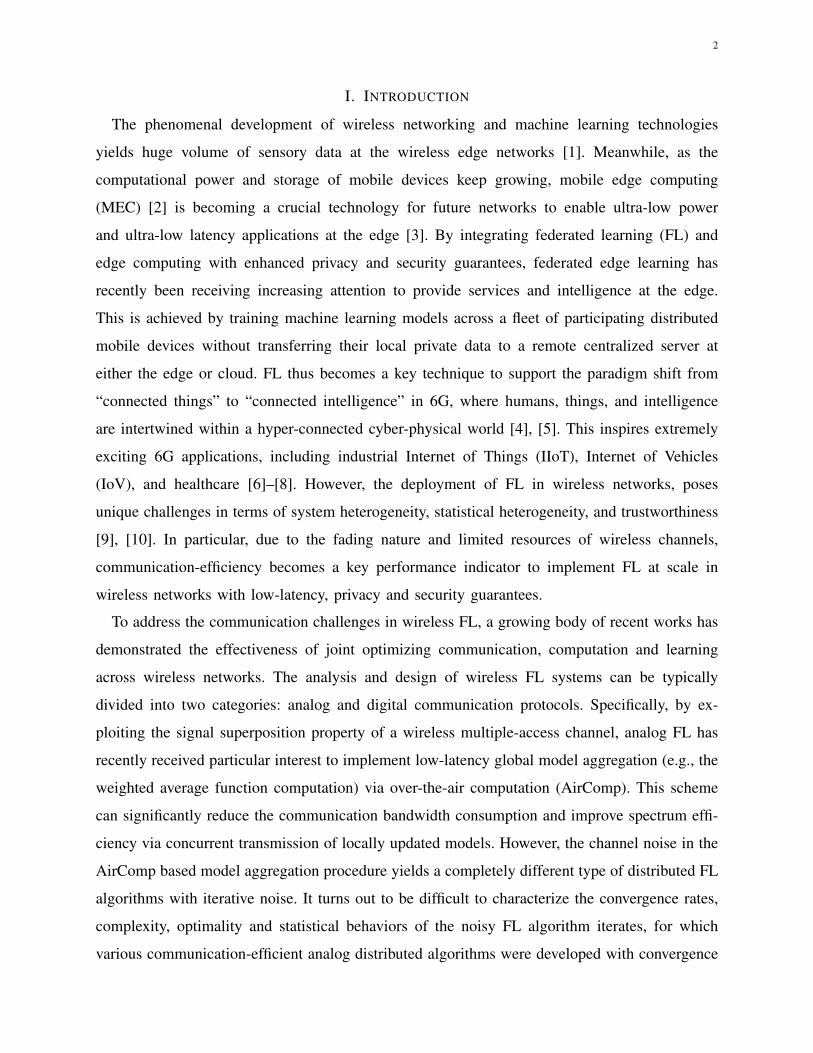
1) Synchronous Downlink Scheme:
The first proposed transmission scheme is the synchronous downlink communication, for
which the downlink delay depends on the worst channel of involved users. Since the BS occupies
2Actually, in Alg. 1, each iteration consists of two rounds of computation and transmission: one round for ∇Lk(w(n)) and
∇L(w(n)), another round for g(n)k and w(n+1). Without loss of generality, we consider only one round of computation and
transmission for the convenience of analysis. Also note that, in this paper, the one iteration delay is denoted by T (n) when itis used as a variable. It can also be written as a function of the number of involved users K in the FL system, i.e., T (n)(K).

9
Fig. 2. The schematic diagram for the synchronous downlink scheme.
more bandwidth to broadcast the global model, the bandwidth for downlink transmission is
denoted by Bdl. The downlink transmission rate at the t-th downlink transmission time slot is
thus given by
r(n)dl (t) = Bdl ln
(1 +
Pdl
(h(n)dl (t)
)2σ2
), (15)
where h(n)dl (t) = min{|h(n)dl,k(t)|, k ∈ K}, Pdl is the transmission power of the BS. In this scheme,
users have the same downlink transmission delay. Therefore, all involved users update their local
models synchronously. The schematic diagram for this scheme is shown in Fig. 2. Accordingly,
the uplink and downlink delays at iteration n in the first scheme are respectively given by
T(n)ul = max{t(n)ul,k, k ∈ K} = T0 max
k∈Kmin
{d : T0
d∑t=1
r(n)ul,k(t) ≥ S, d ∈ N+
}, (16)
T(n)dl = T0 min
{d : T0
d∑t=1
r(n)dl (t) ≥ S, d ∈ N+
}. (17)
As the local computation time t(n)cp,k is a deterministic constant for user k, it has no influence
on the random distribution of the one iteration delay. Moreover, with the rapid development
of both algorithms and hardware, the computational power and efficiency of mobile devices is
growing rapidly. Thus, for simplicity, it is reasonable to assume that t(n)cp,k is much shorter than
the uplink and downlink transmission delay and can be ignored in the following discussions3.
The one iteration delay at iteration n in this scheme is thus given by T (n) = T(n)ul + T
(n)dl .
From the above analysis, we can see that in the synchronous downlink scheme there are two time
alignments among all users during one iteration. The first one is downlink time alignment because
of the synchronous downlink scheme, while the second one is one iteration time alignment
because the global model aggregation can not start until all users’ local model parameters are
uploaded to the BS.
3The reasonability of this assumption will be further proved in Section IV.

10
Fig. 3. The schematic diagram for the asynchronous downlink scheme.
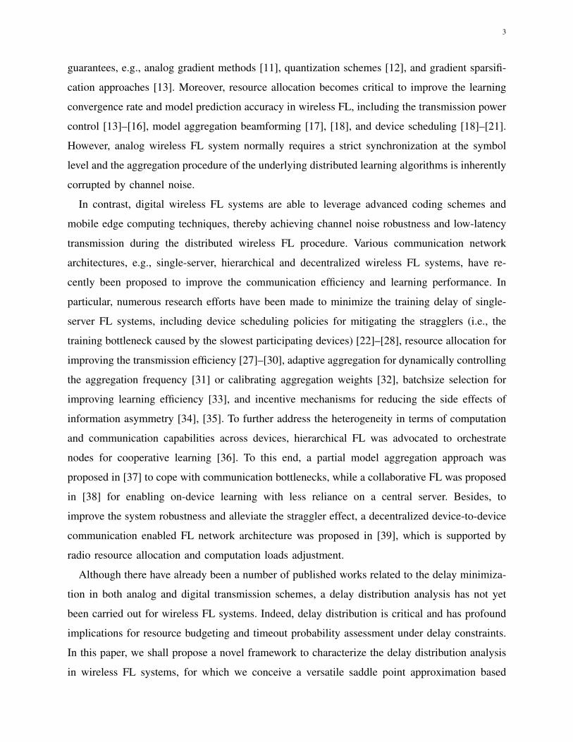
2) Asynchronous Downlink Scheme:
Another proposed transmission scheme is the asynchronous downlink communication, which
is also known as broadcast with common information. This downlink model is equivalent to a
broadcast channel in which a single encoding of a common message is being sent to multiple
receivers, where each experiences a different SNR because of different channel coefficients. By
using rateless coding, users can achieve their capacity simultaneously [46]. Therefore, in this
case, the downlink transmission rate for user k is given by
r(n)dl,k(t) = Bdl ln
(1 +
Pdl|h(n)dl,k(t)|2
σ2
). (18)
In this scheme, the start time of different users’ uplink transmission is asynchronous. Therefore,
as shown in Fig. 3, there is only one time alignment between all users in one iteration. Hence,
one iteration delay in this scheme is given by
T (n) = maxk∈K{T (n)
k : T(n)k = t
(n)ul,k + t
(n)dl,k}
= T0 maxk∈K
min
{d1 + d2 : T0
d1∑t=1
r(n)dl,k(t) ≥ S, T0
d2∑t=1
r(n)ul,k(t) ≥ S; d1, d2 ∈ N+
}, (19)
which is the largest sum of the uplink and downlink transmission delay.
III. DELAY ANALYSIS IN WIRELESS FL SYSTEMS
In this section, we first analyze the distribution of one iteration delay in two proposed
wireless FL transmission schemes by leveraging a saddle point approximation based method
[47]. Based on an upper bound of the iteration numbers for convergence, we also analyze the
overall delay distribution. To get more insights, we use EVT, LDT and stochastic order [48] to
further characterize the properties of the delay distribution in wireless FL systems. Finally, to
overcome the difficulties of obtaining the accurate number of convergence rounds analytically,
we model the number of convergence rounds as a random variable, thereby using an empirical
distribution to further characterize the overall delay in wireless FL systems.
11
A. One Iteration Delay Distribution of the Synchronous Downlink Scheme
For the synchronous downlink scheme, we investigate the uplink delay and downlink delay
presented in Section II. To derive the uplink delay distribution of the wireless FL system, we
conceive a saddle point approximation based method, in which the Lugannani-Rice (LR) formula
[49] and differential analysis are leveraged to get one user’s uplink delay distribution in Lemma 1,
followed by presenting the distribution of the system’s uplink delay in Theorem 1. For simplicity,
we assume that the mean of the channel coefficients is√π/2. Moreover, we assume that the
transmit power of all involved users is fixed, for which we let λ = Pkσ2 and λd = Pdl
σ2 in the
following derivations.
Lemma 1. Define Zd as
Zd =
SBT0
, d = 0,
SBT0−∑d
t=1
r(n)ul,k(t)
B, d ≥ 1.
(20)
For all d ≥ 1, the distribution of user k’s uplink delay t(n)ul,k can be expressed as
%(d)=Pr{t(n)ul,k=dT0
}=
1√2π
(∫ ωd
ωd−1
e−u2
2 du+e−ω2d−1
2
( 1
ψd−1− 1
ωd−1
)−e−
ω2d2
( 1
ψd− 1
ωd
)), (21)
where ωd = sign(s∗d)√−2Kd
(s∗d), ψd = s∗d
√K ′′d(s∗d)
for d ≥ 1, and ω0 = ψ0 = −∞. Kd(s) is
the Cumulant Generating Function (CGF) of Zd, which is given in (22). Here, s∗d is the solution
to K ′d(s∗d)
= 0, which satisfies (23).
Kd(s) =S
BT0s+ d ln
(e
12λ (2λ)−sΓ
(− s+ 1,
erth
2λ
)). (22)
S
BT0=
dG3,02,3
(0, 0
−s∗d,−1,−1
∣∣∣∣∣ 12λ
)2λΓ(−s∗d + 1, 1
2λ)
. (23)
In (22)-(23), Γ(s, x) ,∫ +∞x
ts−1e−tdt is the upper incomplete gamma function [50] and
Gρ1,ρ2ρ3,ρ4
(a1, a2, . . . , aρ3
b1, b2, . . . , bρ4
∣∣∣∣∣z)
=1
2πi
∮L
∏ρ1j=1 Γ(bj − h)
∏ρ2j=2 Γ(1− aj + h)∏ρ4
j=ρ1+1 Γ(1− bj + h)∏ρ3
j=ρ2+1 Γ(aj − h)zhdh (24)
is the Meijer G-function [51].
Proof: Please refer to Appendix A for details.
Theorem 1. Given the distribution of t(n)ul,k, the system’s uplink delay distribution in the
synchronous downlink scheme is given by

12
ϕ(d) = Pr{T
(n)ul = dT0
}=
(1√2π
∫ ωd
−∞e−
u2
2 du− e−ω2d2
√2π
( 1
ψd− 1
ωd
))K
−(
1√2π
∫ ωd−1
−∞e−
u2
2 du− e−ω2d−1
2
√2π
( 1
ψd−1− 1
ωd−1
))K. (25)
Proof: Please refer to Appendix B for details.
The distribution of the downlink delay in the synchronous downlink scheme can be derived
similarly from the uplink delay analysis. It is given in the following lemma.
Lemma 2. Define Zd as
Zd =
S
BdlT0, d = 0,
SBdlT0
−∑d
t=1
r(n)dl (t)
Bdl, d ≥ 1.
(26)
For all d ≥ 1, the downlink delay distribution in the synchronous downlink scheme is given by
υ(d)=Pr{T
(n)dl =dT0
}=
1√2π
(∫ ωd
ωd−1
e−u2
2 du+ e−ω2d−1
2
( 1
ψd−1− 1
ωd−1
)−e−
ω2d2
( 1
ψd− 1
ωd
)), (27)
where ωd=sign(s∗d)√−2Kd
(s∗d), ψd= s∗d
√K ′′d(s∗d)
for d ≥ 1, and ω0 = ψ0 =−∞. Kd(s) is the
CGF of Zd, which is given in (28). Here, s∗d is the solution to K ′d(s∗d)
= 0, which satisfies (29).
Kd(s) =S
BdlT0s+ d ln
(eK2λd
(2λdK
)−sΓ(− s+ 1,
K
2λd
)). (28)
S
BdlT0=
dKG3,02,3
(0, 0
−s∗d,−1,−1
∣∣∣∣∣ K2λd)
2λdΓ(−s∗d + 1, K2λd
). (29)
Proof: Please refer to Appendix C for details.
Based on Theorem 1 and Lemma 2, we are ready to obtain the distribution of one iteration
delay in the synchronous downlink scheme in the following theorem.
Theorem 2. Given the uplink and downlink delay distribution, the distribution of one iteration
delay in the synchronous downlink scheme can be obtained as
Pr{T (n) = dT0
}=
d−1∑i=1
ϕ(i) υ(d− i)
=1√2π
d−1∑i=1
[(1√2π
∫ ωi
−∞e−
u2
2 du− e−ω2i2
√2π
( 1
ψi− 1
ωi
))K−(
1√2π
∫ ωi−1
−∞e−
u2
2 du− e−ω2i−1
2
√2π( 1
ψi−1− 1
ωi−1
))K][∫ ωd−i
ωd−i−1
e−u2
2 du+e−ω2d−i−1
2
( 1
ψd−i−1− 1
ωd−i−1
)−e−
ω2d−i2
( 1
ψd−i− 1
ωd−i
)]. (30)
13
Proof: As presented in Section II-A, in the synchronous downlink scheme, T (n) = T(n)ul +
T(n)dl . Therefore, given the uplink delay distribution and the downlink delay distribution, the
distribution of one iteration delay T (n) is the convolution of distributions of T (n)ul and T
(n)dl ,
which is shown in (30).
Corollary 1. When the number of users K approaches infinity, define R(t) as
R(t) = T0
⌈ tT0
⌉− t+
∑∞d=d t
T0e(1−
∑dj=1
∑j−1i=1 %(i)υ(j − i)
)1−
∑b tT0c
j=1
∑j−1i=1 %(i)υ(j − i)
, (31)
where d·e is the ceiling functions, b·c is the floor function. For all real x, if
limt→+∞
1−∑b t+xR(t)
T0c
j=1
∑j−1i=1 %(i)υ(j − i)
1−∑b t
T0c
j=1
∑j−1i=1 %(i)υ(j − i)
= e−x, (32)
then the limiting distribution of T (n) is given by
Pr{T (n) < y
}= e−e
− y−ab , (33)
where a and b can be chosen as
a = inf
{x : 1−
b xT0c∑
j=1
j−1∑i=1
%(i)υ(j − i) ≤ 1
K
}, (34)
b = R(a). (35)
Proof: Please refer to Appendix D for details.
In Corollary 1, we use EVA to characterize the asymptotic property of one iteration delay
in the synchronous downlink scheme. In practical scenarios, the number of users in a wireless
system is usually large. Hence, we can use Corollary 1 to simplify the computation. Note that,
this analysis is also applicable to the one iteration delay in the asynchronous downlink scheme.
B. One Iteration Delay Distribution of the Asynchronous Downlink Scheme
The analysis of one iteration delay for the asynchronous downlink scheme has some simi-
larities with the synchronous one in Section III-A. First, we give the distribution of t(n)dl,k in the
asynchronous downlink scheme in Lemma 3. Furthermore, the distribution of one iteration delay
in the asynchronous downlink scheme will be presented in Theorem 3.
Lemma 3. Define Zd as
Zd =
S
BdlT0, d = 0,
SBdlT0
−∑d
t=1
r(n)dl,k(t)
Bdl, d ≥ 1.
(36)
For all d ≥ 1, the distribution of t(n)dl,k in the asynchronous downlink scheme is given by
ϑ(d)=Pr{t(n)dl,k=dT0
}=
1√2π
(∫ ωd
ωd−1
e−u2
2 du+e−ω2d−1
2
( 1
ψd−1− 1
ωd−1
)−e−
ω2d2
( 1
ψd− 1
ωd
)), (37)
14
where ωd=sign(s∗d)√−2Kd
(s∗d), ψd= s∗d
√K ′′d(s∗d)
for d ≥ 1, and ω0 = ψ0 =−∞. Kd(s) is the
CGF of Zd, which is given in (38). Here, s∗d is the solution to K ′d(s∗d)
= 0, which satisfies (39).
Kd(s) =S
BdlT0s+ d ln
(e
12λd (2λd)
−sΓ(− s+ 1,
1
2λd
)). (38)
S
BdlT0=
dG3,02,3
(0, 0
−s∗d,−1,−1
∣∣∣∣∣ 12λd
)2λdΓ(−s∗d + 1, 1
2λd)
. (39)
Proof: This derivation is similar to Lemma 1. Except for the SNR varying from λ to λd,
the only difference is related to the bandwidth which becomes Bdl.
Theorem 3. The distribution of one iteration delay in the asynchronous downlink scheme is
given by
Pr{T (n) = dT0
}=
( d∑j=1
j−1∑i=1
%(i)ϑ(j − i))K−( d−1∑
j=1
j−1∑i=1
%(i)ϑ(j − i))K
. (40)
Proof: Please refer to Appendix E for details.
Corollary 2. When the number of users K approaches infinity, define m(t) as
m(t) = T0
⌈ tT0
⌉− t+
∑∞d=d t
T0e(1−
∑dj=1
∑j−1i=1 %(i)ϑ(j − i)
)1−
∑b tT0c
j=1
∑j−1i=1 %(i)ϑ(j − i)
. (41)
For all real x, if
limt→+∞
1−∑b t+xm(t)
T0c
j=1
∑j−1i=1 %(i)ϑ(j − i)
1−∑b t
T0c
j=1
∑j−1i=1 %(i)ϑ(j − i)
= e−x, (42)
then the limiting distribution of T (n) is given by
Pr{T (n) < y
}= e−e
− y−ab , (43)
where a and b can be chosen as
a = inf
{x : 1−
b xT0c∑
j=1
j−1∑i=1
%(i)ϑ(j − i) ≤ 1
K
}, (44)
b = m(a). (45)
Proof: Please refer to Appendix F for details.
C. Overall Delay Analysis
It is challenging to drive the exact number of iterations for the distributed FL algorithms,
for which we adopt the results in [29] presented in Lemma 4. It gives an upper bound of the
iteration numbers needed for Alg. 1 to achieve convergence.
Lemma 4. Assume that the loss function Lk(w) satisfies:
(a) Lk(w) is α-smooth, i.e., ∇2Lk(w) � αI .
(b) Lk(w) is γ-strongly convex, i.e., ∇2Lk(w) � γI .
15
Under these assumptions, if we run Alg. 1 with 0 < ξ ≤ γα
and µ = 0 for
n ≥ u
1− η, I0 (46)
iterations with u = 2α2
γ2ξln 1
ε0, we have L(w(n))− L(w?) ≤ ε0
(L(w(0))− L(w?)
).
Proof: Please refer to [29] Appendix A for details.
The assumptions in Theorem 3 are widely used in the literature for FL convergence analysis
[22], [23], [27]–[29], [31]. Note that, Lemma 4 is established on the condition that µ = 0, which
seems like abandoning the regularization term. However, if we put the regularization term into
Lk(w), which means we define Lk(w) as the sum of the local loss and the regularization term,
the conclusion in Lemma 4 still holds.
Having the upper bound of the number of iterations, we analyze the tail distribution of Tc for
different schemes by LDT in the following Theorems 4 and 5, respectively.
Theorem 4. For τ > I0E{T (n)}, if the CGF of T (n) exists, the tail distribution of Tc in the
synchronous downlink scheme can be expressed as
Pr{Tc ≥ τ} = exp
(− s?τ + I0 ln
( ∞∑d=1
es?dT0
d−1∑i=1
ϕ(i)υ(d− i)))
, (47)
where s? satisfies ∑∞d=1 dT0e
s?dT0∑d−1
i=1 ϕ(i)υ(d− i)∑∞d=1 e
s?dT0∑d−1
i=1 ϕ(i)υ(d− i)=
τ
I0. (48)
Proof: Please refer to Appendix G for details.
By the same way, we can get the property of Tc’s tail distribution in the asynchronous downlink
scheme in Theorem 5.
Theorem 5. For τ > I0E{T (n)}, if the CGF of T (n) exists, the tail distribution of Tc in the
asynchronous downlink scheme can be expressed as
Pr{Tc≥τ}=exp
(−s?τ+I0 ln
( ∞∑d=1
es?dT0[( d∑
j=1
j−1∑i=1
%(i)ϑ(j−i))K−(d−1∑
j=1
j−1∑i=1
%(i)ϑ(j−i))K]))
, (49)
where s? satisfies∑∞d=1 dT0e
s?dT0[(∑d
j=1
∑j−1i=1 %(i)ϑ(j − i))K − (
∑d−1j=1
∑j−1i=1 %(i)ϑ(j − i)
)K]∑∞d=1 e
s?dT0[(∑d
j=1
∑j−1i=1 %(i)ϑ(j − i))K − (
∑d−1j=1
∑j−1i=1 %(i)ϑ(j − i)
)K] =τ
I0. (50)
Corollary 3. The time needed for the convergence of the training process is less than the sum
of I0 iteration delays in the stochastic order
Tc =N−1∑i=0
T (i) ≤stI0−1∑i=0
T (i). (51)
Proof: Since Tc =∑N−1
i=0 T (i) and N ≤ I0, we have Pr{Tc > t} ≤ Pr{∑I0−1
i=0 T (i) > t} for
all t > 0.
16
Combined the EVT on one iteration delay with Theorem 4 and Theorem 5, we can get the
following asymptotic results for the distribution of overall delay in wireless FL systems when
the number of involved users approaches infinity.
Theorem 6. When the number of users in the wireless FL system K approaches infinity, if
the conditions in (32) and (42) are satisfied, then for τ > I0E[T (n)], the tail distribution of Tc
can be further expressed as
Pr{Tc ≥ τ} = exp(−s?τ)
(eab−e
ab
b
∫ +∞
0
e(s?− 1
b)ye−e
− 1by
dy
)I0, (52)
where a and b are chosen differently according to the different downlink schemes from (34),
(35) or (44), (45), while s? satisfies (48) or (50) according to the downlink schemes, too.
Proof: Please refer to Appendix H for details.
It turns out that machine learning models especially deep learning models may not always
satisfy the assumptions in Lemma 4. It is thus difficult to find the globally optimal solution for
nonconvex machine learning models. In fact, the distributed learning procedures and models used
in wireless FL systems become extremely complicated. As mentioned in Section I, the systems
and statistical heterogeneity in wireless FL systems brings additional difficulties to perform the
exact analysis on N . Therefore, by modeling N as a random variable, we can instead use the
empirical distribution to characterize it. Specifically, we define the probability generating function
(PGF) of non-negative discrete random variable of the number of iterations N as
GN(z) =∞∑n=0
Pr{N = n}zn, (53)
where Pr{N = n} can be approximated by the frequency of N = n in massive independently
repeated experiments according to the law of large numbers [48]. Similarly, the PGF of one
iteration delay T (n) is given by
GI(z) =∞∑i=0
Pr{T (n) = iT0
}zi, (54)
where Pr{T (n) = iT0
}can be derived from (30) in the synchronous downlink transmission
scheme or (40) in the asynchronous downlink transmission scheme. Since the overall delay Tc
is a compound random variable of N and T (n), now we can characterize the distribution of Tc
based on GN(z) and GI(z) in the following corollary.
Corollary 4. Given the PGF GN(z) of the iteration number for convergence N and GI(z) of
the one iteration delay T (n), the overall delay distribution can be expressed as
Pr{Tc = dT0} =G
(d)N
(GI(z)
)∣∣z=0
d!, (55)
17
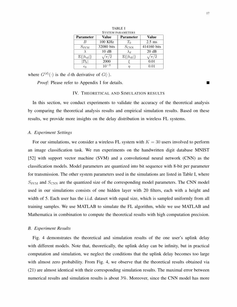
TABLE ISYSTEM PARAMETERS
Parameter Value Parameter ValueB 100 KHz T0 2.5 ms
SSVM 32080 bits SCNN 414160 bitsλ 10 dB λd 20 dB
E{|hul|}√π/2 E{|hdl|}
√π/2
|Dk| 2000 ξ 0.01ε0 10−3 η 0.01
where G(d)(·) is the d-th derivative of G(·).
Proof: Please refer to Appendix I for details.
IV. THEORETICAL AND SIMULATION RESULTS
In this section, we conduct experiments to validate the accuracy of the theoretical analysis
by comparing the theoretical analysis results and empirical simulation results. Based on these
results, we provide more insights on the delay distribution in wireless FL systems.
A. Experiment Settings
For our simulations, we consider a wireless FL system with K = 30 users involved to perform
an image classification task. We run experiments on the handwritten digit database MNIST
[52] with support vector machine (SVM) and a convolutional neural network (CNN) as the
classification models. Model parameters are quantized into bit sequence with 8-bit per parameter
for transmission. The other system parameters used in the simulations are listed in Table I, where
SSVM and SCNN are the quantized size of the corresponding model parameters. The CNN model
used in our simulations consists of one hidden layer with 20 filters, each with a height and
width of 5. Each user has the i.i.d. dataset with equal size, which is sampled uniformly from all
training samples. We use MATLAB to simulate the FL algorithm, while we use MATLAB and
Mathematica in combination to compute the theoretical results with high computation precision.
B. Experiment Results
Fig. 4 demonstrates the theoretical and simulation results of the one user’s uplink delay
with different models. Note that, theoretically, the uplink delay can be infinity, but in practical
computation and simulation, we neglect the conditions that the uplink delay becomes too large
with almost zero probability. From Fig. 4, we observe that the theoretical results obtained via
(21) are almost identical with their corresponding simulation results. The maximal error between
numerical results and simulation results is about 3%. Moreover, since the CNN model has more
18
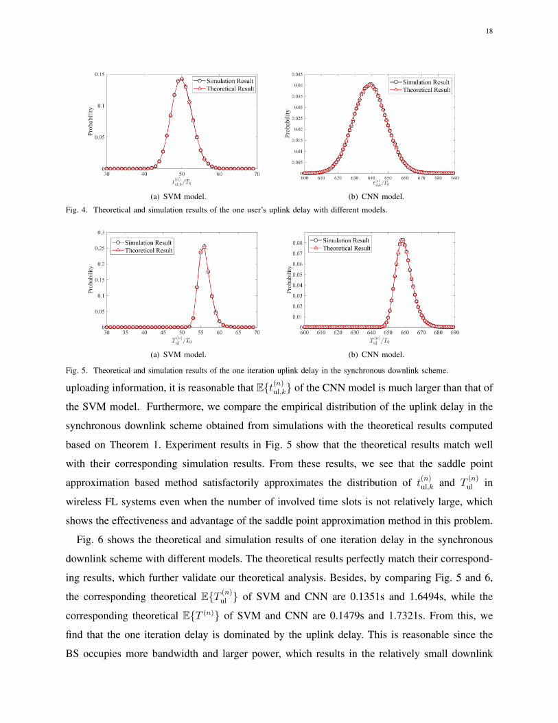
(a) SVM model. (b) CNN model.
Fig. 4. Theoretical and simulation results of the one user’s uplink delay with different models.
(a) SVM model. (b) CNN model.
Fig. 5. Theoretical and simulation results of the one iteration uplink delay in the synchronous downlink scheme.
uploading information, it is reasonable that E{t(n)ul,k} of the CNN model is much larger than that of
the SVM model. Furthermore, we compare the empirical distribution of the uplink delay in the
synchronous downlink scheme obtained from simulations with the theoretical results computed
based on Theorem 1. Experiment results in Fig. 5 show that the theoretical results match well
with their corresponding simulation results. From these results, we see that the saddle point
approximation based method satisfactorily approximates the distribution of t(n)ul,k and T(n)ul in
wireless FL systems even when the number of involved time slots is not relatively large, which
shows the effectiveness and advantage of the saddle point approximation method in this problem.
Fig. 6 shows the theoretical and simulation results of one iteration delay in the synchronous
downlink scheme with different models. The theoretical results perfectly match their correspond-
ing results, which further validate our theoretical analysis. Besides, by comparing Fig. 5 and 6,
the corresponding theoretical E{T (n)ul } of SVM and CNN are 0.1351s and 1.6494s, while the
corresponding theoretical E{T (n)} of SVM and CNN are 0.1479s and 1.7321s. From this, we
find that the one iteration delay is dominated by the uplink delay. This is reasonable since the
BS occupies more bandwidth and larger power, which results in the relatively small downlink
19
(a) SVM model. (b) CNN model.
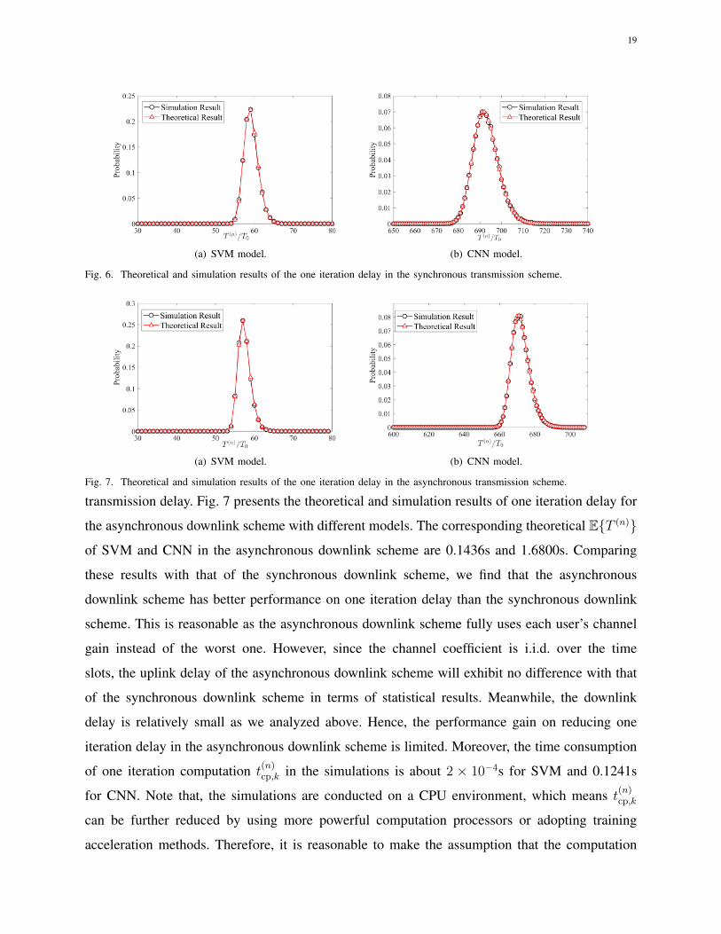
Fig. 6. Theoretical and simulation results of the one iteration delay in the synchronous transmission scheme.
(a) SVM model. (b) CNN model.
Fig. 7. Theoretical and simulation results of the one iteration delay in the asynchronous transmission scheme.
transmission delay. Fig. 7 presents the theoretical and simulation results of one iteration delay for
the asynchronous downlink scheme with different models. The corresponding theoretical E{T (n)}
of SVM and CNN in the asynchronous downlink scheme are 0.1436s and 1.6800s. Comparing
these results with that of the synchronous downlink scheme, we find that the asynchronous
downlink scheme has better performance on one iteration delay than the synchronous downlink
scheme. This is reasonable as the asynchronous downlink scheme fully uses each user’s channel
gain instead of the worst one. However, since the channel coefficient is i.i.d. over the time
slots, the uplink delay of the asynchronous downlink scheme will exhibit no difference with that
of the synchronous downlink scheme in terms of statistical results. Meanwhile, the downlink
delay is relatively small as we analyzed above. Hence, the performance gain on reducing one
iteration delay in the asynchronous downlink scheme is limited. Moreover, the time consumption
of one iteration computation t(n)cp,k in the simulations is about 2 × 10⁻⁴s for SVM and 0.1241s
for CNN. Note that, the simulations are conducted on a CPU environment, which means t(n)cp,k
can be further reduced by using more powerful computation processors or adopting training
acceleration methods. Therefore, it is reasonable to make the assumption that the computation
20
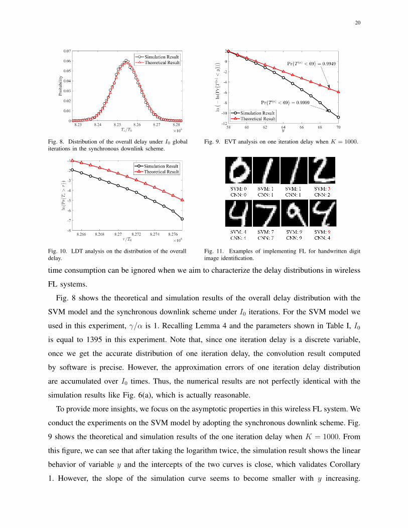
Fig. 8. Distribution of the overall delay under I0 globaliterations in the synchronous downlink scheme.
Fig. 9. EVT analysis on one iteration delay when K = 1000.
Fig. 10. LDT analysis on the distribution of the overalldelay.
Fig. 11. Examples of implementing FL for handwritten digitimage identification.
time consumption can be ignored when we aim to characterize the delay distributions in wireless
FL systems.
Fig. 8 shows the theoretical and simulation results of the overall delay distribution with the
SVM model and the synchronous downlink scheme under I0 iterations. For the SVM model we
used in this experiment, γ/α is 1. Recalling Lemma 4 and the parameters shown in Table I, I0
is equal to 1395 in this experiment. Note that, since one iteration delay is a discrete variable,
once we get the accurate distribution of one iteration delay, the convolution result computed
by software is precise. However, the approximation errors of one iteration delay distribution
are accumulated over I0 times. Thus, the numerical results are not perfectly identical with the
simulation results like Fig. 6(a), which is actually reasonable.
To provide more insights, we focus on the asymptotic properties in this wireless FL system. We
conduct the experiments on the SVM model by adopting the synchronous downlink scheme. Fig.
9 shows the theoretical and simulation results of the one iteration delay when K = 1000. From
this figure, we can see that after taking the logarithm twice, the simulation result shows the linear
behavior of variable y and the intercepts of the two curves is close, which validates Corollary
1. However, the slope of the simulation curve seems to become smaller with y increasing.

21
(a) SVM model. (b) CNN model.
Fig. 12. The frequency distribution histogram of iteration numbers for convergence.
(a) SVM model. (b) CNN model.
Fig. 13. The overall delay distribution in the synchronous downlink scheme.
The reason is that the number of simulations is not probably large enough to reflect the true
distribution of T (n), while the twice logarithm operation magnifies the difference between them.
Fig. 10 represents the theoretical and simulation results of the overall delay under I0 iterations.
By taking the logarithm, the slope of simulation results is approximately identical with the
theoretical one, which validates Theorem 4. When τ is large, the slope becomes smaller, which
means Pr{Tc ≥ τ} decays faster than the exponential distributions.
Fig. 11 persents performance results of the proposed FL algorithm for handwritten digit
identification. Fig. 12 is the frequency distribution histogram of the number of iterations for
convergence. In Fig. 12(a), we can see that all numbers are less than a threshold in this simulation
for SVM, which proves that Lemma 4 has some significance. Moreover, from Fig. 12(b), we
can see that although CNN does not meet the assumption mentioned in Lemma 4, it shows the
same property with the result of SVM. However, since CNN is a nonconvex model, it may not
converge. Although probability is rather small to be ignored in the simulation, N can be infinity

22
in theory, which means there may not be an upper bound for nonconvex models. Hence, by
taking all of the above factors into account, it is reasonable to treat N as a random variable.
Fig. 13 represents both the empirical and theoretical distribution of the overall delay in the
synchronous downlink scheme with different models. The difference between the empirical result
and the theoretical result is slightly more evident compared to Fig. 6. It is due to the fact that we
use the empirical distribution of N obtained in Fig. 12 to get the overall delay distribution, which
magnifies the errors. However, the results in Fig. 13 still show that the empirical distributions of
the overall delay are in good agreement with the theoretical distributions. From this experiment,
we see that it is practical to calculate the generating function of N through its empirical
distribution. Nonetheless, it is clear that getting more accurate distribution of global iteration
numbers remains an open and challenging problem.
V. CONCLUSIONS
In this paper, we investigated the delay distribution for wireless FL systems.
In particular, synchronous and asynchronous downlink transmission schemes were further
proposed in wireless FL systems, followed by the definitions of the one iteration and overall
delay. To characterize the accurate approximation and asymptotic properties of delay distributions
in wireless FL systems, saddle point approximation, EVT and LDT methods were exploited.
Moreover, we proposed to model the convergence rounds as a random variable instead of a
constant, yielding a novel way to provide an empirical distribution for the overall delay in
wireless FL systems. The proposed modeling and analytical tools for the delay distribution
provide a novel research direction to better understand and design wireless FL systems in both
practical and theoretical aspects. Future promising research directions include improving the
resource efficiency and users’ experience by leveraging the presented analytical results in this
paper.
APPENDIX A
PROOF OF LEMMA 1
According to (9), we have
t(n)ul,k = T0
{d :
d∑t=1
r(n)ul,k(t) ≥
S
T0,
d−1∑t=1
r(n)ul,k(t) <
S
T0, d ∈ N+
}, (56)
Pr{t(n)ul,k > dT0
}= Pr
{d∑t=1
r(n)ul,k(t) <
S
T0
}. (57)

23
Since r(n)ul,k(t) derives from (14), where h(n)ul,k(t) is i.i.d. over n and t, for simplicity, we omit
n and t in the following derivation in this paper. According to the definition of Zd in (20), (56)
and (57) can be rewritten as
tul,k = {dT0 : Zd ≤ 0, Zd−1 > 0, d ∈ N+}. (58)
Pr{tul,k > dT0} = Pr{Zd > 0}. (59)
Then we obtain
Pr{tul,k = dT0} = Pr{tul,k > (d− 1)T0} − P{tul,k > dT0}
= Pr{Zd−1 > 0} − Pr{Zd > 0}. (60)
From (60), we see that if we want to obtain the distribution of tul,k, we need to get the
complementary cumulative distribution function (CCDF) of Zd first. However, we can not get
the distribution of Zd easily, since it is hard to obtain the distribution of∑d
t=1 rul,k by convolution.
Therefore, we turn to saddle point approximation to obtain an accurate approximation of Zd’s
CCDF.
CGF is defined as the natural logarithm of moment generating function (MGF). Hence, the
CGF of Zd is given byKd(s) = lnE
{esZd
}=
S
BT0s+ lnE
{e−s
∑dt=1 rul,kB
}=
S
BT0s+ d lnE
{e−
srul,kB
}. (61)
Similar to MGF, CGF allows us to obtain the n-th cumulant of Zd by evaluating its n-th derivative
at zero. The first two cumulants are the mean and the variance.
Having the CGF of Zd, we need to find the saddle point s∗d. Since we want to obtain Pr{Zd >
0}, we have to solve the following saddle point equation:
K′
d
(s∗d)
= 0. (62)
Then the CCDF of Zd can be approximated by the first two terms of the LR formula as
Pr{Zd > 0} = 1− 1√2π
∫ ωd
−∞e−
u2
2 du+e−
ω2d2
√2π
( 1
ψd− 1
ωd
). (63)
The ωd and ψd, for d ≥ 1, are defined as
ωd = sign(s∗d)√−2Kd
(s∗d), (64)
ψd = s∗d
√K ′′d(s∗d), (65)
where sign(·) is the sign function. When d = 0, Pr{Z0 > 0} = 1. To keep the definition rigorous,
we let ω0 = ψ0 = −∞.
24
Given that |hul,k| follows Rayleigh distribution fh(x) = xe−x2
2 , we can express the distribution
of rul,kB
asful(r) =
1
2λe
12λ er−
er
2λ I{r ≥ 0}, (66)
where I{·} is the indicator function.
According to the definition of MGF, the MGF of rul,kB
is given by
M(s) =
∫ +∞
−∞esrful(r)dr
= e12λ (2λ)sΓ
(s+ 1,
1
2λ
). (67)
Thus, substituting (67) into (61), we have
Kd(s) =S
BT0s+ d lnM(−s)
=S
BT0s+ d ln
(e
12λ (2λ)−sΓ
(− s+ 1,
1
2λ
)). (68)
Then we can obtain the first and second derivative of Kd(s) respectively as
K ′d(s) =S
BT0− dM
′(−s)M(−s)
, (69)
K ′′d (s) = dM ′′(−s)M(−s)
− d(M ′(−s)
)2(M(−s)
)2 . (70)
M ′(−s) and M ′′(−s) are given by
M ′(−s) = e12λ (2λ)−s
[ln (2λ)Γ
(− s+ 1,
1
2λ
)+ Γ′
(− s+ 1,
1
2λ
)], (71)
M ′′(−s)=e12λ (2λ)−s
[ln2 (2λ)Γ
(−s+1,
1
2λ
)+2 ln (2λ)Γ′
(−s+1,
1
2λ
)+Γ′′
(−s+1,
1
2λ
)], (72)
where Γ′(·) and Γ′′(·) are given by
Γ′(− s+ 1,
1
2λ
)= Γ
(− s+ 1,
1
2λ
)ln( 1
2λ
)+
1
2λG3,0
2,3
(0, 0
−s,−1,−1
∣∣∣∣∣ 1
2λ
), (73)
Γ′′(− s+ 1,
1
2λ
)= Γ
(− s+ 1,
1
2λ
)ln2( 1
2λ
)+
1
λ
[G4,0
3,4
(0, 0, 0
−s,−1,−1,−1
∣∣∣∣∣ 1
2λ
)
+ ln( 1
2λ
)G3,0
2,3
(0, 0
−s,−1,−1
∣∣∣∣∣ 1
2λ
)]. (74)
In (73) and (74), Gρ1,ρ2ρ3,ρ4
(a1, a2, . . . , aρ3
b1, b2, . . . , bρ4
∣∣∣∣∣z)
is the Meijer G-function, which is defined in (24).
Combined with (62), (69), (71) and (73), we can know that the parameter s∗d satisfies the

25
following equation:
S
BT0=
dG3,02,3
(0, 0
−s∗d,−1,−1
∣∣∣∣∣ 12λ
)2λΓ(−s∗d + 1, 1
2λ)
. (75)
Once we get s∗d, ωd = sign(s∗d)√−2Kd
(s∗d)
can be obtained from (68). Moreover, ψd =
s∗d√K ′′d (s∗d) can also be obtained by using (70), (71), (72), (73), and (74). Hence, according to
the LR formula, we can approximate the probability Pr{Zd > 0} by (63). Substituting (63) into
(60), the distribution of one user’s uplink time slots consumption is obtained as (21) shows.
APPENDIX B
PROOF OF THEOREM 1
As shown in (16), we notice that Tul is the maximum order statistic between one user’s uplink
delay tul,k. Therefore, the probability of Tul = dT0 is equal to that of max{tul,k, k ∈ K} = dT0,
which is given by
Pr{
max{tul,k, k ∈ K} = dT0}
=K∏k=1
Pr{tul,k ≤ dT0} −K∏k=1
Pr{tul,k ≤ (d− 1)T0}. (76)
Recalling (59), Pr{tul,k ≤ dT0} = 1 − Pr{Zd > 0}. Hence, substituting (63) into (76), the
distribution of Tul can be expressed as
Pr{Tul = dT0} =(1− Pr{Zd > 0}
)K − (1− Pr{Zd−1 > 0})K.
=
(1√2π
∫ ωd
−∞e−
u2
2 du− e−ω
2d2
√2π
( 1
ψd− 1
ωd
))K−(
1√2π
∫ ωd−1
−∞e−
u2
2 du− e−ω2d−1
2
√2π
( 1
ψd−1− 1
ωd−1
))K.
(77)APPENDIX C
PROOF OF LEMMA 2
Similar to the proof of Lemma 1, we can use saddle point approximation to get the distribution
of T (n)dl . Specifically, there is a difference between uplink and downlink rate distribution. Since
hdl = min{|hdl,k|, k ∈ K}, we can get the distribution of hdl, which is given by
fhdl(x) = K[1− Fh(x)
]K−1fh(x)
= Kxe−Kx2
2 I{x > 0}, (78)
where Fh(x) =(1− e−x
2
2
)I{x > 0} is the CDF of |hdl,k|. Based on (78), the distribution of rdl
Bdl
is given by
fdl(r) =K
2λdeK2λd e
r− K2λd
erI{r ≥ 0}, (79)
26
where λd = Pdl
σ2 is the corresponding SNR.
Then the MGF of rdlBdl
is given by
Mdl(s) = eK2λd
(2λdK
)sΓ(s+ 1,
K
2λd
). (80)
The CGF of Zd is given by
Kd(s) =S
BdlT0s+ d lnMdl(−s)
=S
BdlT0s+ d ln
[eK2λd
(2λdK
)−sΓ(− s+ 1,
K
2λd
)]. (81)
Comparing (81) with (68), we can see that if we let λ = λdK
, then the further derivation is similar
to the derivation of the uplink delay. Thus, we omit it due to the limitation of layout. Finally,
the distribution of Tdl is given as shown in (27).
APPENDIX D
PROOF OF COROLLARY 1
Let F (·) denote the CDF of the user k’s one iteration delay T (n)k , which is given by
F (x) =
b xT0c∑
j=1
j−1∑i=1
%(i)υ(j − i). (82)
Then the one iteration delay of the FL system can be expressed as T (n) = max{T
(n)k , k ∈ K
}.
From [40], we can know that, if the limiting distribution of T (n) exists, it must belong to one
of the three standard extreme value distributions: Frechet, Weibull and Gumbel distribution. The
distribution of T (n)k determines the limiting distribution of T (n). Therefore, according to Theorem
2.13 in [40] and [53], we can give the sufficient condition for the distribution of T (n) satisfying
Gumbel distribution.
Let w(F ) denote the upper endpoint of F (x), which is given by
w(F ) = sup{x : F (x) < 1}. (83)
Based on the definition of T (n)k , we can know that the w(F ) = ∞. Hence, if there exist some
finite b satisfy ∫ +∞
b
(1− F (y)
)dy < +∞, (84)
then for 0 < t < +∞, we define
R(t) =
∫ +∞t
(1− F (y)
)dy
1− F (t)= T0
⌈ tT0
⌉− t+
∑∞d=d t
T0e(1−
∑dj=1
∑j−1i=1 %(i)υ(j − i)
)1−
∑b tT0c
j=1
∑j−1i=1 %(i)υ(j − i)
, (85)
which is also known as mean residual life function. For all real x, if

27
limt→+∞
1− F(t+ xR(t)
)1− F (t)
= limt→+∞
1−∑b t+xR(t)
T0c
j=1
∑j−1i=1 %(i)υ(j − i)
1−∑b t
T0c
j=1
∑j−1i=1 %(i)υ(j − i)
= e−x, (86)
then there are sequences an and bn > 0 such that, −∞ < x <∞,
limK→+∞
Pr{T (n)(K) < aK + bKx
}= e−e
−x. (87)
The constants aK and bK can be chosen as
aK = inf
{x : 1− F (x) ≤ 1
K
}, (88)
bK = R(aK). (89)
APPENDIX E
PROOF OF THEOREM 3
To get the distribution of T (n) in the asynchronous downlink scheme, we need to get the one
user’s delay first, then we take the maximum order statistic of all user’s delay. Similar to the
synchronous downlink scheme, one user’s uplink delay can be obtained by Lemma 1. Moreover,
one user’s downlink delay is given in Lemma 3. Thus, the delay of user k in one iteration is
given as the convolution of the uplink delay and downlink delay
Pr{T
(n)k = dT0
}=
d−1∑i=1
Pr{t(n)ul,k = iT0
}Pr{t(n)dl,k = (d− i)T0
}=
d−1∑i=1
%(i)ϑ(d− i). (90)
By substituting (21), (37) into (90), the corresponding distribution is given by
Pr{T (n) = dT0
}=
K∏k=1
Pr{T
(n)k ≤ dT0
}−
K∏k=1
Pr{T
(n)k ≤ (d− 1)T0
}=
( d∑j=1
j−1∑i=1
%(i)ϑ(j − i))K−( d−1∑
j=1
j−1∑i=1
%(i)ϑ(j − i))K
. (91)
APPENDIX F
PROOF OF COROLLARY 2
The most parts of the derivation are similar to Corollary 1. The difference lies in the CDF of
T(n)k . In the asynchronous downlink scheme, the CDF of T (n)
k is given by
F (x) =
b xT0c∑
j=1
j−1∑i=1
%(i)ϑ(j − i). (92)
Then we can get a similar result as derived from Corollary 1.
28
APPENDIX G
PROOF OF THEOREM 4
Our proof relies on the LDT. Having the distribution of the one iteration delay T (n), we can
analyze the tail distribution of Tc by LDT. Based on Theorem 23.3 in [41], first we calculate
the CGF of T (n) as
K(s) = lnE{esT
(n)}= ln
( ∞∑d=1
esdT0d−1∑i=1
ϕ(i)υ(d− i)). (93)
Then the rate function I(s), which is the Legendre transform of K(s), is given by
Λ∗(x) = sups∈R
(sx−K(s)
)= s?x− ln
( ∞∑d=1
es?dT0
d−1∑i=1
ϕ(i)υ(d− i)), (94)
where s? can be calculated as∑∞d=1 dT0e
s?dT0∑d−1
i=1 ϕ(i)υ(d− i)∑∞d=1 e
s?dT0∑d−1
i=1 ϕ(i)υ(d− i)= x. (95)
Then, for every x > E{T (n)},
limn→∞
1
nln Pr
{ n∑i=1
T (i) ≥ xn
}= −Λ∗(x). (96)
Hence, for x > E{T (n)} and n→∞, the tail distribution of Tc can be expressed as
Pr{Tc ≥ xn} = e−n(s?x−ln
(∑∞d=1 e
s?dT0∑d−1i=1 ϕ(i)υ(d−i)
)). (97)
Recalling that I0 is the upper bound of n, it can be seen as a relatively large number. Hence,
for τ ≥ I0E{T (n)}, by inserting n = I0 and τ = xI0, (47) holds.
APPENDIX H
PROOF OF THEOREM 6
According to (33) and (43), the probability density function of T (n) when K approaches
infinity is given by
f(y) =1
be−
y−ab−e−
y−ab . (98)
Then similar to the derivation in Theorem 4, we can get
K(s) = − ln b+a
b− e
ab + ln
(∫ +∞
0
e(s−1b)ye−e
− 1by
dy
), (99)
Λ∗(x) = sups∈R
(sx−K(s)
)= s?x− ln
(∫ +∞
0
e(s?− 1
b)ye−e
− 1by
dy
)+ ln b− a
b+ e
ab , (100)
where s? satisfies ∫ +∞
0
ye(s?− 1
b)ye−e
− 1by
dy = x
∫ +∞
0
e(s?− 1
b)ye−e
− 1by
dy. (101)

29
Hence, for τ ≥ I0E{T (n)}, the tail distribution of Tc can be expressed as
Pr{Tc ≥ τ} = exp
(− I0
(s?x− ln
(∫ +∞
0
e(s?− 1
b−e−
1b )ydy
)+ ln b− a
b+ e
ab
))
= exp(−s?τ)
(eab−e
ab
b
∫ +∞
0
e(s?− 1
b)ye−e
− 1by
dy
)I0. (102)
APPENDIX I
PROOF OF COROLLARY 4
Once we get the distribution of the number of iterations for convergence N , we obtain its
PGF GN(z). From Theorem 2 and Theorem 3, we can also get the PGF of one iteration delay,
which we denote as GI(z). Therefore, the MGF of overall delay is given by
Gc(z) =∞∑d=1
zdT0 Pr{Tc = dT0}
=∞∑j=1
Pr{N = j}∞∑d=1
Pr{Tc = dT0|N = j}zdT0
=∞∑j=1
Pr{N = j}(GI(z)
)j= GN
(GI(z)
). (103)
Based on the Gc(z), we can derive the distribution of Tc from
Pr{Tc = dT0} =G
(d)c (0)
d!=G
(d)n
(GI(z)
)∣∣z=0
d!. (104)
REFERENCES
[1] G. Zhu, D. Liu, Y. Du, C. You, J. Zhang, and K. Huang, “Toward an intelligent edge: Wireless communication meetsmachine learning,” IEEE Commun. Mag., vol. 58, no. 1, pp. 19–25, Jan. 2020.
[2] Y. Mao, C. You, J. Zhang, K. Huang, and K. B. Letaief, “A survey on mobile edge computing: The communicationperspective,” IEEE Commun. Surveys Tuts., vol. 19, no. 4, pp. 2322–2358, Aug. 2017.
[3] Y. Shi, K. Yang, T. Jiang, J. Zhang, and K. B. Letaief, “Communication-efficient edge AI: Algorithms and systems,” IEEECommun. Surveys Tuts., vol. 22, no. 4, pp. 2167–2191, Jul. 2020.
[4] K. B. Letaief, W. Chen, Y. Shi, J. Zhang, and Y. A. Zhang, “The roadmap to 6G: AI empowered wireless networks,” IEEECommun. Mag., vol. 57, no. 8, pp. 84–90, Aug. 2019.
[5] W. Saad, M. Bennis, and M. Chen, “A vision of 6G wireless systems: Applications, trends, technologies, and open researchproblems,” IEEE Netw., vol. 34, no. 3, pp. 134–142, May 2020.
[6] S. Niknam, H. S. Dhillon, and J. H. Reed, “Federated learning for wireless communications: Motivation, opportunities,and challenges,” IEEE Commun. Mag., vol. 58, no. 6, pp. 46–51, Jun. 2020.
[7] W. Y. B. Lim, N. C. Luong, D. T. Hoang, Y. Jiao, Y. C. Liang, Q. Yang, D. Niyato, and C. Miao, “Federated learning inmobile edge networks: A comprehensive survey,” IEEE Commun. Surveys Tuts., vol. 22, no. 3, pp. 2031–2063, Apr. 2020.
[8] Y. Sun, W. Shi, X. Huang, S. Zhou, and Z. Niu, “Edge learning with timeliness constraints: Challenges and solutions,”IEEE Commun. Mag., vol. 58, no. 12, pp. 27–33, Dec. 2020.
[9] L. U. Khan, S. R. Pandey, N. H. Tran, W. Saad, Z. Han, M. N. H. Nguyen, and C. S. Hong, “Federated learning for edgenetworks: Resource optimization and incentive mechanism,” IEEE Commun. Mag., vol. 58, no. 10, pp. 88–93, Nov. 2020.
[10] T. Li, A. K. Sahu, A. Talwalkar, and V. Smith, “Federated learning: Challenges, methods, and future directions,” IEEESignal Process. Mag., vol. 37, no. 3, pp. 50–60, May 2020.
[11] T. Sery and K. Cohen, “On analog gradient descent learning over multiple access fading channels,” IEEE Trans. SignalProcess., vol. 68, pp. 2897–2911, Apr. 2020.
[12] G. Zhu, Y. Du, D. Gunduz, and K. Huang, “One-bit over-the-air aggregation for communication-efficient federated edgelearning: Design and convergence analysis,” IEEE Trans. Wireless Commun., pp. 1–1, Nov. 2020.
[13] M. M. Amiri and D. Gunduz, “Federated learning over wireless fading channels,” IEEE Trans. Wireless Commun., vol. 19,no. 5, pp. 3546–3557, May 2020.
30
[14] X. Wei and C. Shen, “Federated learning over noisy channels: Convergence analysis and design examples,” 2021,arXiv:2101.02198. [Online]. Available: https://arxiv.org/abs/2101.02198
[15] D. Liu, and O. Simeone, “Privacy for Free: Wireless Federated Learning via Uncoded Transmission With Adaptive PowerControl,” IEEE J. Sel. Areas Commun., vol. 39, no. 1, pp. 170–185, Jan. 2021.
[16] X. Cao, G. Zhu, J. Xu, and K. Huang, “Optimized Power Control for Over-the-Air Computation in Fading Channels,”IEEE Trans. Wireless Commun., vol. 19, no. 11, pp. 7498–7513, Nov. 2020.
[17] M. M. Amiri, T. M. Duman, D. Gunduz, S. R. Kulkarni, and H. V. Poor, “Blind federated edge learning,” 2020,arXiv:2010.10030. [Online]. Available: https://arxiv.org/abs/2010.10030
[18] K. Yang, T. Jiang, Y. Shi, and Z. Ding, “Federated learning via over-the-air computation,” IEEE Trans. Wireless Commun.,vol. 19, no. 3, pp. 2022–2035, Mar. 2020.
[19] G. Zhu, Y. Wang, and K. Huang, “Broadband analog aggregation for low-latency federated edge learning,” IEEE Trans.Wireless Commun., vol. 19, no. 1, pp. 491–506, Jan. 2020.
[20] H. Liu, X. Yuan, and Y.-J. A. Zhang, “Reconfigurable intelligent surface enabled federated learning: A unifiedcommunication-learning design approach,” 2020, arXiv:2011.10282. [Online]. Available: https://arxiv.org/abs/2011.10282
[21] S. Xia, J. Zhu, Y. Yang, Y. Zhou, Y. Shi, and W. Chen, “Fast convergence algorithm for analog federated learning,” 2020,arXiv:2011.06658. [Online]. Available: https://arxiv.org/abs/2011.06658
[22] H. H. Yang, Z. Liu, T. Q. S. Quek, and H. V. Poor, “Scheduling policies for federated learning in wireless networks,”IEEE Trans. Commun., vol. 68, no. 1, pp. 317–333, Jan. 2020.
[23] J. Ren, Y. He, D. Wen, G. Yu, K. Huang, and D. Guo, “Scheduling for cellular federated edge learning with importanceand channel awareness,” IEEE Trans. Wireless Commun., vol. 19, no. 11, pp. 7690–7703, Nov. 2020.
[24] M. M. Amiri, D. Gunduz, S. R. Kulkarni, and H. Vincent Poor, “Update aware device scheduling for federated learningat the wireless edge,” in Proc. IEEE Int. Symp. Inf. Theory (ISIT), Jun. 2020, pp. 2598–2603.
[25] B. Luo, X. Li, S. Wang, J. Huang, and L. Tassiulas, “Cost-effective federated learning design,” 2020, arXiv:2012.08336.[Online]. Available: https://arxiv.org/abs/2012.08336
[26] B. Buyukates and S. Ulukus, “Timely Communication in Federated Learning,” 2020, arXiv:2012.15831. [Online]. Available:https://arxiv.org/abs/2012.15831
[27] W. Shi, S. Zhou, Z. Niu, M. Jiang, and L. Geng, “Joint device scheduling and resource allocation for latency constrainedwireless federated learning,” IEEE Trans. Wireless Commun., pp. 453–467, Jan. 2021.
[28] M. Chen, Z. Yang, W. Saad, C. Yin, H. V. Poor, and S. Cui, “A joint learning and communications framework for federatedlearning over wireless networks,” IEEE Trans. Wireless Commun., pp. 269–283, Jan. 2021.
[29] Z. Yang, M. Chen, W. Saad, C. S. Hong, and M. Shikh-Bahaei, “Energy efficient federated learning over wirelesscommunication networks,” IEEE Trans. Wireless Commun., pp. 1–1, Nov. 2020.
[30] D. Wen, M. Bennis, and K. Huang, “Joint parameter-and-bandwidth allocation for improving the efficiency of partitionededge learning,” IEEE Trans. Wireless Commun., pp. 8272–8286, Dec. 2020.
[31] S. Wang, T. Tuor, T. Salonidis, K. K. Leung, C. Makaya, T. He, and K. Chan, “Adaptive federated learning in resourceconstrained edge computing systems,” IEEE J. Sel. Areas Commun., vol. 37, no. 6, pp. 1205–1221, Jun. 2019.
[32] H. T. Nguyen, V. Sehwag, S. Hosseinalipour, C. G. Brinton, M. Chiang, and H. Vincent Poor, “Fast-convergent federatedlearning,” IEEE J. Sel. Areas Commun., pp. 201–218, Jan. 2021.
[33] J. Ren, G. Yu, and G. Ding, “Accelerating DNN training in wireless federated edge learning systems,” IEEE J. Sel. AreasCommun., vol. 39, no. 1, pp. 219–232, Jan. 2021.
[34] S. R. Pandey, N. H. Tran, M. Bennis, Y. K. Tun, Z. Han, and C. S. Hong, “Incentivize to build: A crowdsourcing frameworkfor federated learning,” in Proc. IEEE Global Commun. Conf. (GLOBECOM), Dec. 2019, pp. 1–6.
[35] N. Ding, Z. Fang, and J. Huang, “Optimal contract design for efficient federated learning with multi-dimensional privateinformation,” IEEE J. Sel. Areas Commun., vol. 39, no. 1, pp. 186–200, Jan. 2021.
[36] S. Hosseinalipour, C. G. Brinton, V. Aggarwal, H. Dai, and M. Chiang, “From federated to fog learning: Distributedmachine learning over heterogeneous wireless networks,” IEEE Commun. Mag., vol. 58, no. 12, pp. 41–47, Dec. 2020.
[37] L. Liu, J. Zhang, S. H. Song, and K. B. Letaief, “Client-edge-cloud hierarchical federated learning,” in Proc. IEEE Int.Conf. Commun. (ICC), Dublin, Ireland, Jun. 2020, pp. 1–6.
[38] M. Chen, H. V. Poor, W. Saad, and S. Cui, “Wireless communications for collaborative federated learning,” IEEE Commun.Mag., vol. 58, no. 12, pp. 48–54, Dec. 2020.
[39] X. Cai, X. Mo, J. Chen, and J. Xu, “D2D-enabled data sharing for distributed machine learning at wireless network edge,”IEEE Wireless Commun. Lett., vol. 9, no. 9, pp. 1457–1461, Sept. 2020.
[40] J. Galambos, “The asymptotic theory of extreme order statistics,” Tech. Rep., 1978.[41] A. Klenke, Probability theory: a comprehensive course. Springer Science & Business Media, 2013.[42] J. Konecny, H. B. McMahan, D. Ramage, and P. Richtarik, “Federated optimization: Distributed machine learning for
on-device intelligence,” 2016, arXiv:1610.02527. [Online]. Available: https://arxiv.org/abs/1610.02527[43] O. Shamir, N. Srebro, and T. Zhang, “Communication-efficient distributed optimization using an approximate newton-type
method,” in Proc. Int. Conf. Mach. Learn. (ICML), 2014, pp. 1000–1008.[44] H. G. Myung, J. Lim, and D. J. Goodman, “Single carrier FDMA for uplink wireless transmission,” IEEE Veh. Technol.
Mag., vol. 1, no. 3, pp. 30–38, Sept. 2006.[45] Q. Zeng, Y. Du, K. Huang, and K. K. Leung, “Energy-efficient radio resource allocation for federated edge learning,” in
Proc. IEEE Int. Conf. Commun. (ICC) Workshop, Dublin, Ireland, Jun. 2020, pp. 1–6.[46] U. Erez, M. D. Trott, and G. W. Wornell, “Rateless coding for gaussian channels,” IEEE Trans. Inf. Theory, vol. 58, no. 2,
pp. 530–547, Feb. 2012.[47] R. W. Butler, Saddlepoint approximations with applications. Cambridge University Press, 2007, vol. 22.[48] S. M. Ross, J. J. Kelly, R. J. Sullivan, W. J. Perry, D. Mercer, R. M. Davis, T. D. Washburn, E. V. Sager, J. B. Boyce,
and V. L. Bristow, Stochastic processes. Wiley New York, 1996, vol. 2.[49] R. Lugannani and S. Rice, “Saddle point approximation for the distribution of the sum of independent random variables,”
Advances in applied probability, vol. 12, no. 2, pp. 475–490, 1980.[50] M. Abramowitz and I. A. Stegun, Handbook of mathematical functions with formulas, graphs, and mathematical tables.
US Government printing office, 1970, vol. 55.[51] H. Bateman, Higher transcendental functions [volumes i-iii]. McGraw-Hill Book Company, 1953, vol. 1.[52] Y. LeCun, “The MNIST database of handwritten digits,” http://yann. lecun. com/exdb/mnist/, 1998.[53] H. A. David and H. N. Nagaraja, “Order statistics,” Encyclopedia of Statistical Sciences, 2004.


![Energy Efficient Federated Learning Over Wireless … · 2019-11-07 · arXiv:1911.02417v1 [cs.IT] 6 Nov 2019 1 Energy Efficient Federated Learning Over Wireless Communication Networks](https://img.pdfslide.us/doc/110x75/5fac82d954ace821e75f6a90/energy-eficient-federated-learning-over-wireless-2019-11-07-arxiv191102417v1.jpg)