Chapter 7

Definition and properties oftensor products

The DFT, the DCT, and the wavelet transform were all defined as changes ofbasis for vectors or functions of one variable and therefore cannot be directlyapplied to higher dimensional data like images. In this chapter we will introducea simple recipe for extending such one-dimensional schemes to two (and higher)dimensions. The basic ingredient is the tensor product construction. This isa general tool for constructing two-dimensional functions and filters from one-dimensional counterparts. This will allow us to generalise the filtering andcompression techniques for audio to images, and we will also recognise someof the basic operations for images introduced in Chapter 6 as tensor productconstructions.

A two-dimensional discrete function on a rectangular domain, like for exam-ple an image, is conveniently represented in terms of a matrix X with elementsXi,j , and with indices in the ranges 0 ≤ i ≤ M − 1 and 0 ≤ j ≤ N − 1. Oneway to apply filters to X would be to rearrange the matrix into a long vector,column by column. We could then apply a one-dimensional filter to this vectorand then split the resulting vector into columns that can be reassembled backinto a matrix again. This approach may have some undesirable effects near theboundaries between columns. In addition, the resulting computations may berather ineffective. Consider for example the case where X is an N ×N matrixso that the long vector has length N2. Then a linear transformation applied toX involves multiplication with an N2 ×N2-matrix. Each such matrix multipli-cation may require as many as N4 multiplications which is substantial when Nis large.

The concept of tensor products can be used to address these problems. Us-ing tensor products, one can construct operations on two-dimensional functionswhich inherit properties of one-dimensional operations. Tensor products alsoturn out to be computationally efficient.

212

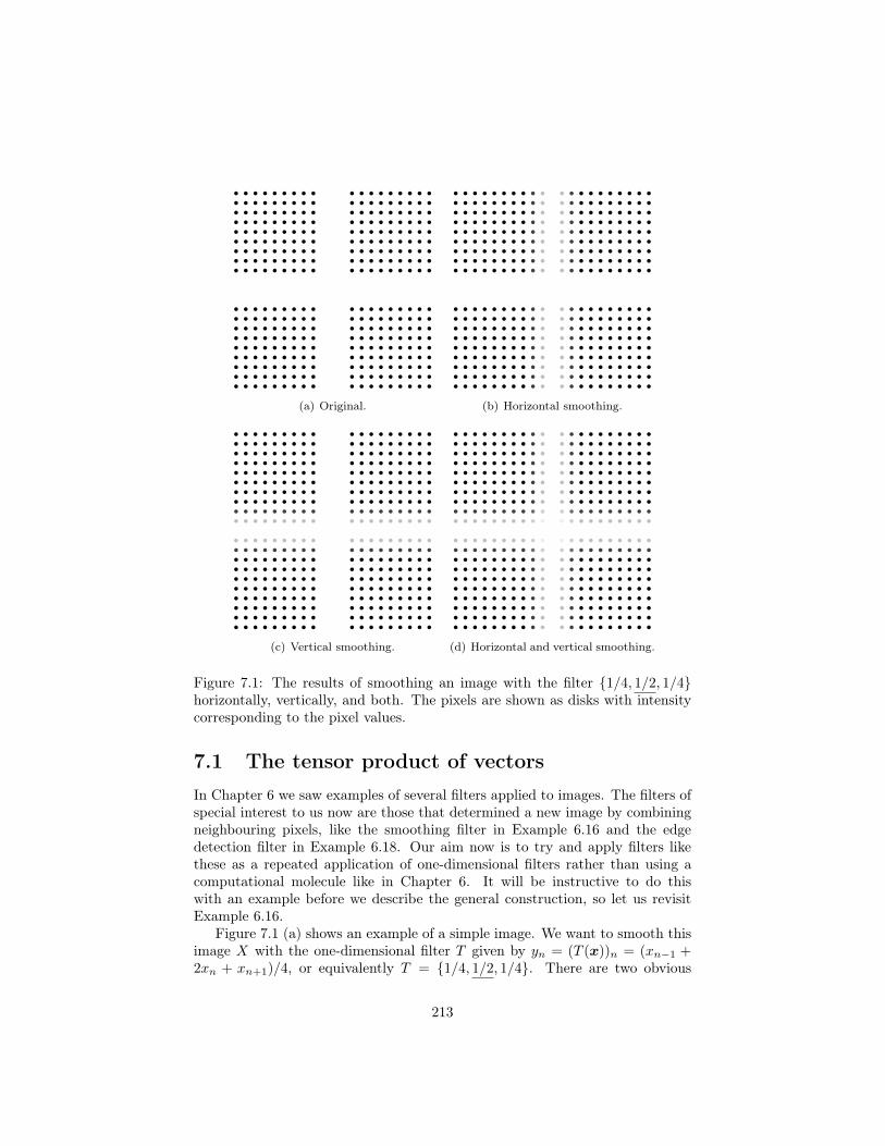
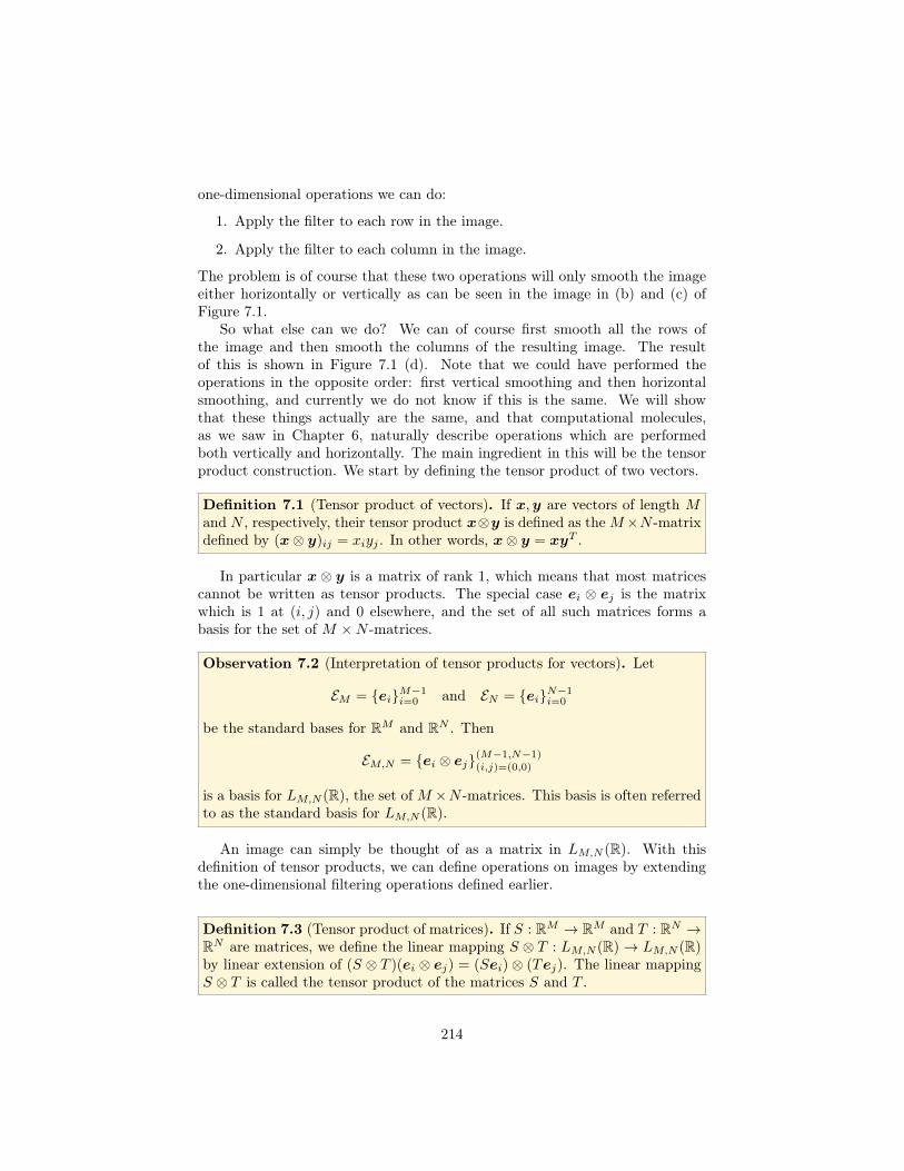
(a) Original. (b) Horizontal smoothing.

(c) Vertical smoothing. (d) Horizontal and vertical smoothing.

Figure 7.1: The results of smoothing an image with the filter {1/4, 1/2, 1/4}horizontally, vertically, and both. The pixels are shown as disks with intensitycorresponding to the pixel values.

7.1 The tensor product of vectorsIn Chapter 6 we saw examples of several filters applied to images. The filters ofspecial interest to us now are those that determined a new image by combiningneighbouring pixels, like the smoothing filter in Example 6.16 and the edgedetection filter in Example 6.18. Our aim now is to try and apply filters likethese as a repeated application of one-dimensional filters rather than using acomputational molecule like in Chapter 6. It will be instructive to do thiswith an example before we describe the general construction, so let us revisitExample 6.16.

Figure 7.1 (a) shows an example of a simple image. We want to smooth thisimage X with the one-dimensional filter T given by yn = (T (x))n = (xn−1 +2xn + xn+1)/4, or equivalently T = {1/4, 1/2, 1/4}. There are two obvious

213

one-dimensional operations we can do:

1. Apply the filter to each row in the image.

2. Apply the filter to each column in the image.

The problem is of course that these two operations will only smooth the imageeither horizontally or vertically as can be seen in the image in (b) and (c) ofFigure 7.1.

So what else can we do? We can of course first smooth all the rows ofthe image and then smooth the columns of the resulting image. The resultof this is shown in Figure 7.1 (d). Note that we could have performed theoperations in the opposite order: first vertical smoothing and then horizontalsmoothing, and currently we do not know if this is the same. We will showthat these things actually are the same, and that computational molecules,as we saw in Chapter 6, naturally describe operations which are performedboth vertically and horizontally. The main ingredient in this will be the tensorproduct construction. We start by defining the tensor product of two vectors.

Definition 7.1 (Tensor product of vectors). If x,y are vectors of length Mand N , respectively, their tensor product x⊗y is defined as the M×N -matrixdefined by (x⊗ y)ij = xiyj . In other words, x⊗ y = xyT .

In particular x ⊗ y is a matrix of rank 1, which means that most matricescannot be written as tensor products. The special case ei ⊗ ej is the matrixwhich is 1 at (i, j) and 0 elsewhere, and the set of all such matrices forms abasis for the set of M ×N -matrices.

Observation 7.2 (Interpretation of tensor products for vectors). Let

EM = {ei}M−1i=0 and EN = {ei}N−1

i=0

be the standard bases for RM and RN . Then

EM,N = {ei ⊗ ej}(M−1,N−1)(i,j)=(0,0)

is a basis for LM,N (R), the set of M ×N -matrices. This basis is often referredto as the standard basis for LM,N (R).

An image can simply be thought of as a matrix in LM,N (R). With thisdefinition of tensor products, we can define operations on images by extendingthe one-dimensional filtering operations defined earlier.

Definition 7.3 (Tensor product of matrices). If S : RM → RM and T : RN →RN are matrices, we define the linear mapping S ⊗ T : LM,N (R) → LM,N (R)by linear extension of (S ⊗ T )(ei ⊗ ej) = (Sei)⊗ (Tej). The linear mappingS ⊗ T is called the tensor product of the matrices S and T .

214

A couple of remarks are in order. First, from linear algebra we know that,when T is linear mapping from V and T (vi) is known for a basis {vi}i of V ,T is uniquely determined. In particular, since the {ei ⊗ ej}i,j form a basis,there exists a unique linear transformation S ⊗ T so that (S ⊗ T )(ei ⊗ ej) =(Sei) ⊗ (Tej). This unique linear transformation is what we call the linearextension from the values in the given basis.

Secondly S ⊗ T also satisfies (S ⊗ T )(x ⊗ y) = (Sx) ⊗ (Ty). This followsfrom

(S ⊗ T )(x⊗ y) = (S ⊗ T )((�

i

xiei)⊗ (�

j

yjej)) = (S ⊗ T )(�

i,j

xiyj(ei ⊗ ej))

=�

i,j

xiyj(S ⊗ T )(ei ⊗ ej) =�

i,j

xiyj(Sei)⊗ (Tej)

=�

i,j

xiyjSei((Tej))T = S(

�

i

xiei)(T (�

j

yjej))T

= Sx(Ty)T = (Sx)⊗ (Ty).

Here we used the result from Exercise 5. Linear extension is necessary anyway,since only rank 1 matrices have the form x⊗ y.

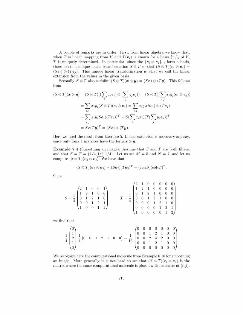
Example 7.4 (Smoothing an image). Assume that S and T are both filters,and that S = T = {1/4, 1/2, 1/4}. Let us set M = 5 and N = 7, and let uscompute (S ⊗ T )(e2 ⊗ e3). We have that

(S ⊗ T )(e2 ⊗ e3) = (Se2)(Te3)T = (col2S)(col3T )T .

Since

S =1

4

2 1 0 0 11 2 1 0 00 1 2 1 00 0 1 2 11 0 0 1 2

T =

1

4

2 1 0 0 0 0 01 2 1 0 0 0 00 1 2 1 0 0 00 0 1 2 1 0 00 0 0 1 2 1 00 0 0 0 1 2 11 0 0 0 0 1 2

,

we find that

1

4

01210

1

4

�0 0 1 2 1 0 0

�=

1

16

0 0 0 0 0 0 00 0 1 2 1 0 00 0 2 4 2 0 00 0 1 2 1 0 00 0 0 0 0 0 0

We recognize here the computational molecule from Example 6.16 for smoothingan image. More generally it is not hard to see that (S ⊗ T )(ei ⊗ ej) is thematrix where the same computational molecule is placed with its centre at (i, j).

215

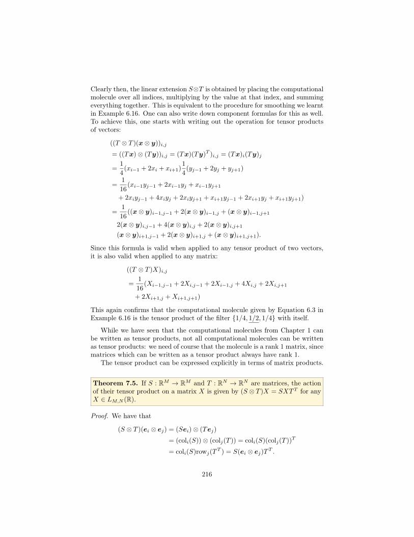
Clearly then, the linear extension S⊗T is obtained by placing the computationalmolecule over all indices, multiplying by the value at that index, and summingeverything together. This is equivalent to the procedure for smoothing we learntin Example 6.16. One can also write down component formulas for this as well.To achieve this, one starts with writing out the operation for tensor productsof vectors:

((T ⊗ T )(x⊗ y))i,j

= ((Tx)⊗ (Ty))i,j = (Tx)(Ty)T )i,j = (Tx)i(Ty)j

=1

4(xi−1 + 2xi + xi+1)

1

4(yj−1 + 2yj + yj+1)

=1

16(xi−1yj−1 + 2xi−1yj + xi−1yj+1

+ 2xiyj−1 + 4xiyj + 2xiyj+1 + xi+1yj−1 + 2xi+1yj + xi+1yj+1)

=1

16((x⊗ y)i−1,j−1 + 2(x⊗ y)i−1,j + (x⊗ y)i−1,j+1

2(x⊗ y)i,j−1 + 4(x⊗ y)i,j + 2(x⊗ y)i,j+1

(x⊗ y)i+1,j−1 + 2(x⊗ y)i+1,j + (x⊗ y)i+1,j+1).

Since this formula is valid when applied to any tensor product of two vectors,it is also valid when applied to any matrix:

((T ⊗ T )X)i,j

=1

16(Xi−1,j−1 + 2Xi,j−1 + 2Xi−1,j + 4Xi,j + 2Xi,j+1

+ 2Xi+1,j +Xi+1,j+1)

This again confirms that the computational molecule given by Equation 6.3 inExample 6.16 is the tensor product of the filter {1/4, 1/2, 1/4} with itself.

While we have seen that the computational molecules from Chapter 1 canbe written as tensor products, not all computational molecules can be writtenas tensor products: we need of course that the molecule is a rank 1 matrix, sincematrices which can be written as a tensor product always have rank 1.

The tensor product can be expressed explicitly in terms of matrix products.

Theorem 7.5. If S : RM → RM and T : RN → RN are matrices, the actionof their tensor product on a matrix X is given by (S ⊗ T )X = SXTT for anyX ∈ LM,N (R).

Proof. We have that

(S ⊗ T )(ei ⊗ ej) = (Sei)⊗ (Tej)

= (coli(S))⊗ (colj(T )) = coli(S)(colj(T ))T

= coli(S)rowj(TT ) = S(ei ⊗ ej)T

T .

216

This means that (S⊗T )X = SXTT for any X ∈ LM,N (R), since equality holdson the basis vectors ei ⊗ ej .

This leads to the following implementation for the tensor product of matrices:

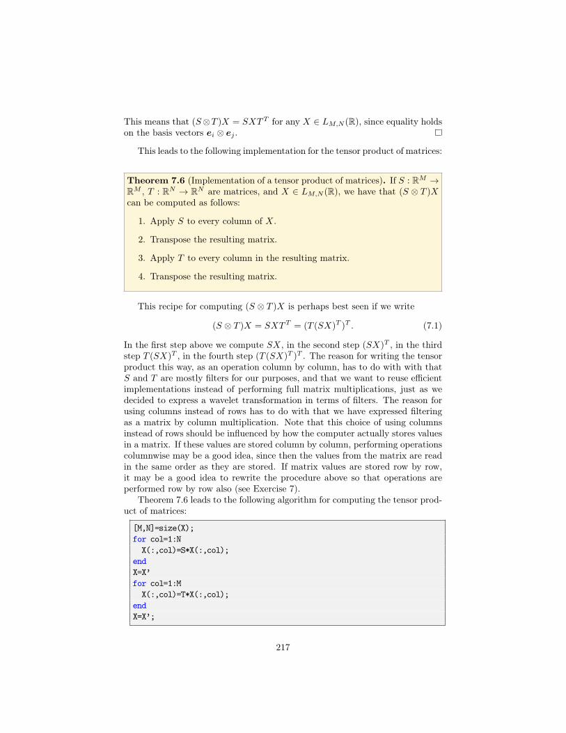
Theorem 7.6 (Implementation of a tensor product of matrices). If S : RM →RM , T : RN → RN are matrices, and X ∈ LM,N (R), we have that (S ⊗ T )Xcan be computed as follows:

1. Apply S to every column of X.

2. Transpose the resulting matrix.

3. Apply T to every column in the resulting matrix.

4. Transpose the resulting matrix.

This recipe for computing (S ⊗ T )X is perhaps best seen if we write

(S ⊗ T )X = SXTT = (T (SX)T )T . (7.1)

In the first step above we compute SX, in the second step (SX)T , in the thirdstep T (SX)T , in the fourth step (T (SX)T )T . The reason for writing the tensorproduct this way, as an operation column by column, has to do with with thatS and T are mostly filters for our purposes, and that we want to reuse efficientimplementations instead of performing full matrix multiplications, just as wedecided to express a wavelet transformation in terms of filters. The reason forusing columns instead of rows has to do with that we have expressed filteringas a matrix by column multiplication. Note that this choice of using columnsinstead of rows should be influenced by how the computer actually stores valuesin a matrix. If these values are stored column by column, performing operationscolumnwise may be a good idea, since then the values from the matrix are readin the same order as they are stored. If matrix values are stored row by row,it may be a good idea to rewrite the procedure above so that operations areperformed row by row also (see Exercise 7).

Theorem 7.6 leads to the following algorithm for computing the tensor prod-uct of matrices:

[M,N]=size(X);for col=1:NX(:,col)=S*X(:,col);

endX=X’for col=1:MX(:,col)=T*X(:,col);

endX=X’;

217

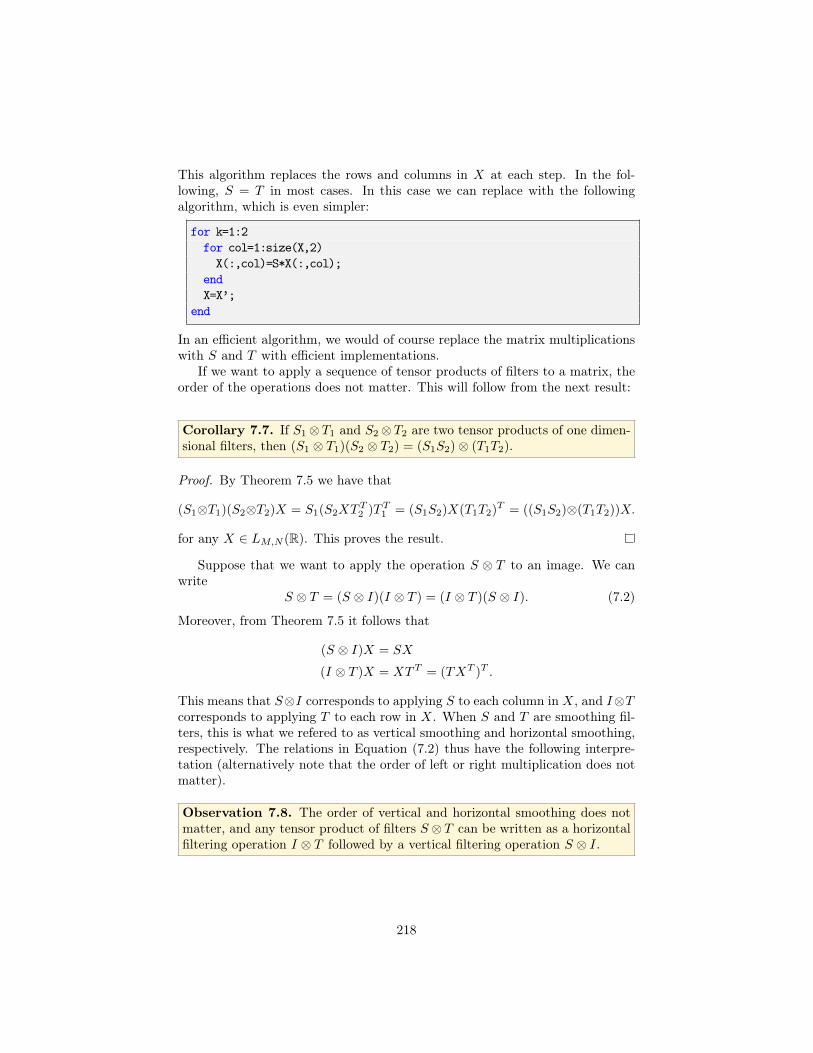
This algorithm replaces the rows and columns in X at each step. In the fol-lowing, S = T in most cases. In this case we can replace with the followingalgorithm, which is even simpler:

for k=1:2for col=1:size(X,2)X(:,col)=S*X(:,col);

endX=X’;

end

In an efficient algorithm, we would of course replace the matrix multiplicationswith S and T with efficient implementations.

If we want to apply a sequence of tensor products of filters to a matrix, theorder of the operations does not matter. This will follow from the next result:

Corollary 7.7. If S1 ⊗T1 and S2 ⊗T2 are two tensor products of one dimen-sional filters, then (S1 ⊗ T1)(S2 ⊗ T2) = (S1S2)⊗ (T1T2).

Proof. By Theorem 7.5 we have that

(S1⊗T1)(S2⊗T2)X = S1(S2XTT2 )TT

1 = (S1S2)X(T1T2)T = ((S1S2)⊗(T1T2))X.

for any X ∈ LM,N (R). This proves the result.

Suppose that we want to apply the operation S ⊗ T to an image. We canwrite

S ⊗ T = (S ⊗ I)(I ⊗ T ) = (I ⊗ T )(S ⊗ I). (7.2)

Moreover, from Theorem 7.5 it follows that

(S ⊗ I)X = SX

(I ⊗ T )X = XTT = (TXT )T .

This means that S⊗I corresponds to applying S to each column in X, and I⊗Tcorresponds to applying T to each row in X. When S and T are smoothing fil-ters, this is what we refered to as vertical smoothing and horizontal smoothing,respectively. The relations in Equation (7.2) thus have the following interpre-tation (alternatively note that the order of left or right multiplication does notmatter).

Observation 7.8. The order of vertical and horizontal smoothing does notmatter, and any tensor product of filters S ⊗ T can be written as a horizontalfiltering operation I ⊗ T followed by a vertical filtering operation S ⊗ I.

218

In fact, the order of any vertical operation S ⊗ I and horizontal operationI ⊗ T does not matter: it is not required that the operations are filters. Forfilters we have a stronger result: If S1, T1, S2, T2 all are filters, we have fromCorollary 7.7 that (S1 ⊗ T1)(S2 ⊗ T2) = (S2 ⊗ T2)(S1 ⊗ T1), since all filterscommute. This does not hold in general since general matrices do not commute.

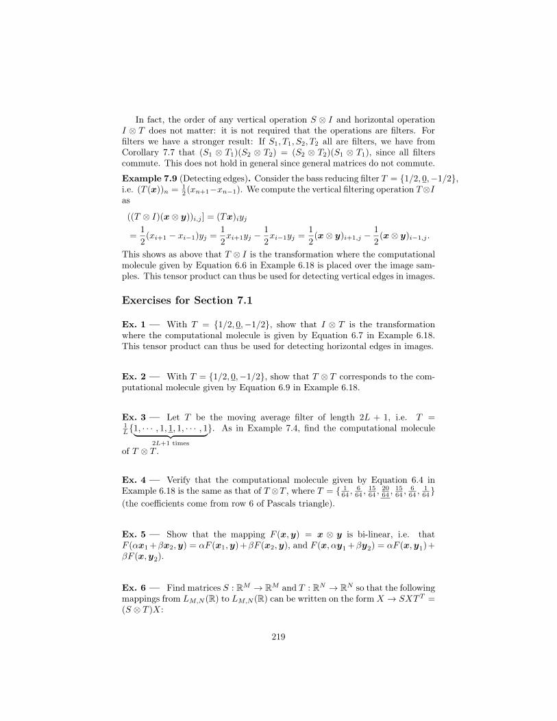
Example 7.9 (Detecting edges). Consider the bass reducing filter T = {1/2, 0,−1/2},i.e. (T (x))n = 1

2 (xn+1−xn−1). We compute the vertical filtering operation T⊗Ias

((T ⊗ I)(x⊗ y))i,j ] = (Tx)iyj

=1

2(xi+1 − xi−1)yj =

1

2xi+1yj −

1

2xi−1yj =

1

2(x⊗ y)i+1,j −

1

2(x⊗ y)i−1,j .

This shows as above that T ⊗ I is the transformation where the computationalmolecule given by Equation 6.6 in Example 6.18 is placed over the image sam-ples. This tensor product can thus be used for detecting vertical edges in images.

Exercises for Section 7.1

Ex. 1 — With T = {1/2, 0,−1/2}, show that I ⊗ T is the transformationwhere the computational molecule is given by Equation 6.7 in Example 6.18.This tensor product can thus be used for detecting horizontal edges in images.

Ex. 2 — With T = {1/2, 0,−1/2}, show that T ⊗ T corresponds to the com-putational molecule given by Equation 6.9 in Example 6.18.

Ex. 3 — Let T be the moving average filter of length 2L + 1, i.e. T =1L{1, · · · , 1, 1, 1, · · · , 1� �� �

2L+1 times

}. As in Example 7.4, find the computational molecule

of T ⊗ T .

Ex. 4 — Verify that the computational molecule given by Equation 6.4 inExample 6.18 is the same as that of T ⊗T , where T = { 1

64 ,664 ,

1564 ,

2064 ,

1564 ,

664 ,

164}

(the coefficients come from row 6 of Pascals triangle).

Ex. 5 — Show that the mapping F (x,y) = x ⊗ y is bi-linear, i.e. thatF (αx1+βx2,y) = αF (x1,y)+βF (x2,y), and F (x,αy1+βy2) = αF (x,y1)+βF (x,y2).

Ex. 6 — Find matrices S : RM → RM and T : RN → RN so that the followingmappings from LM,N (R) to LM,N (R) can be written on the form X → SXTT =(S ⊗ T )X:

219

a. The mapping which reverses the order of the rows in a matrix.b. The mapping which reverses the order of the columns in a matrix.c. The mapping which transposes a matrix.

Ex. 7 — Find an alternative form for Equation (7.1) and an accompanyingreimplementation of Theorem 7.6 which is adapted to the case when we wantall operations to be performed row by row, instead of column by column.

7.2 Change of bases in tensor productsIn this section we will prove a specialization of our previous result to the casewhere S and T are change of coordinate matrices. We start by proving thefollowing:

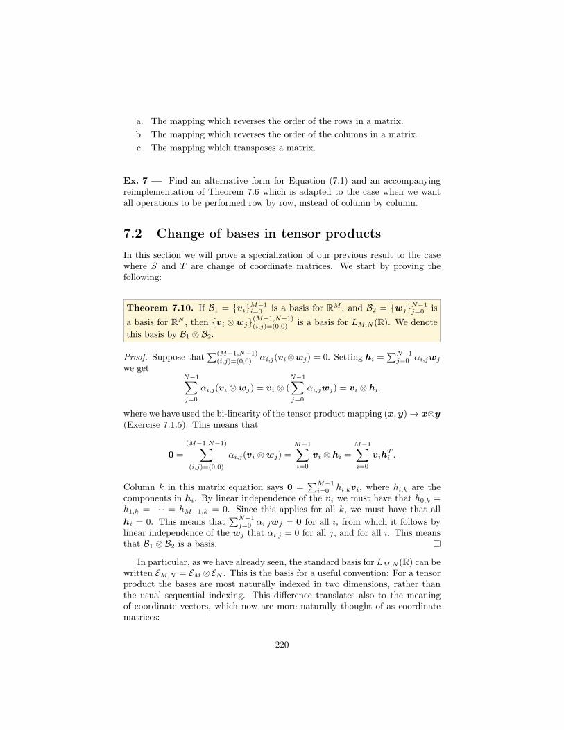
Theorem 7.10. If B1 = {vi}M−1i=0 is a basis for RM , and B2 = {wj}N−1

j=0 isa basis for RN , then {vi ⊗wj}(M−1,N−1)

(i,j)=(0,0) is a basis for LM,N (R). We denotethis basis by B1 ⊗ B2.

Proof. Suppose that�(M−1,N−1)

(i,j)=(0,0) αi,j(vi⊗wj) = 0. Setting hi =�N−1

j=0 αi,jwj

we getN−1�

j=0

αi,j(vi ⊗wj) = vi ⊗ (N−1�

j=0

αi,jwj) = vi ⊗ hi.

where we have used the bi-linearity of the tensor product mapping (x,y) → x⊗y(Exercise 7.1.5). This means that

0 =

(M−1,N−1)�

(i,j)=(0,0)

αi,j(vi ⊗wj) =M−1�

i=0

vi ⊗ hi =M−1�

i=0

vihTi .

Column k in this matrix equation says 0 =�M−1

i=0 hi,kvi, where hi,k are thecomponents in hi. By linear independence of the vi we must have that h0,k =h1,k = · · · = hM−1,k = 0. Since this applies for all k, we must have that allhi = 0. This means that

�N−1j=0 αi,jwj = 0 for all i, from which it follows by

linear independence of the wj that αi,j = 0 for all j, and for all i. This meansthat B1 ⊗ B2 is a basis.

In particular, as we have already seen, the standard basis for LM,N (R) can bewritten EM,N = EM ⊗EN . This is the basis for a useful convention: For a tensorproduct the bases are most naturally indexed in two dimensions, rather thanthe usual sequential indexing. This difference translates also to the meaningof coordinate vectors, which now are more naturally thought of as coordinatematrices:

220

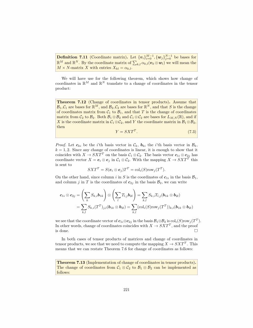
Definition 7.11 (Coordinate matrix). Let {vi}M−1i=0 , {wj}N−1

j=0 be bases forRM and RN . By the coordinate matrix of

�k,l αk,l(vk⊗wl) we will mean the

M ×N -matrix X with entries Xkl = αk,l.

We will have use for the following theorem, which shows how change ofcoordinates in RM and RN translate to a change of coordinates in the tensorproduct:

Theorem 7.12 (Change of coordinates in tensor products). Assume thatB1, C1 are bases for RM , and B2, C2 are bases for RN , and that S is the changeof coordinates matrix from C1 to B1, and that T is the change of coordinatesmatrix from C2 to B2. Both B1⊗B2 and C1⊗C2 are bases for LM,N (R), and ifX is the coordinate matrix in C1⊗C2, and Y the coordinate matrix in B1⊗B2,then

Y = SXTT . (7.3)

Proof. Let cki be the i’th basis vector in Ck, bki the i’th basis vector in Bk,k = 1, 2. Since any change of coordinates is linear, it is enough to show that itcoincides with X → SXTT on the basis C1 ⊗ C2. The basis vector c1i ⊗ c2j hascoordinate vector X = ei ⊗ ej in C1 ⊗ C2. With the mapping X → SXTT thisis sent to

SXTT = S(ei ⊗ ej)TT = coli(S)rowj(T

T ).

On the other hand, since column i in S is the coordinates of c1i in the basis B1,and column j in T is the coordinates of c2j in the basis B2, we can write

c1i ⊗ c2j =

��

k

Sk,ib1k

�⊗

��

l

Tl,jb2l

�=

�

k,l

Sk,iTl,j(b1k ⊗ b2l)

=�

k,l

Sk,i(TT )j,l(b1k ⊗ b2l) =

�

k,l

(coli(S)rowj(TT ))k,l(b1k ⊗ b2l)

we see that the coordinate vector of c1i⊗c2j in the basis B1⊗B2 is coli(S)rowj(TT ).In other words, change of coordinates coincides with X → SXTT , and the proofis done.

In both cases of tensor products of matrices and change of coordinates intensor products, we see that we need to compute the mapping X → SXTT . Thismeans that we can restate Theorem 7.6 for change of coordinates as follows:

Theorem 7.13 (Implementation of change of coordinates in tensor products).The change of coordinates from C1 ⊗ C2 to B1 ⊗ B2 can be implemented asfollows:

221

1. For every column in the coordinate matrix in C1 ⊗ C2, perform a changeof coordinates from C1 to B1.

2. Transpose the resulting matrix.

3. For every column in the resulting matrix, perform a change of coordinatesfrom C2 to B2.

4. Transpose the resulting matrix.

We can reuse the algorithm from the previous section to implement this. Inthe following operations on images, we will visualize the pixel values in an imageas coordinates in the standard basis, and perform a change of coordinates.

Example 7.14 (Change of coordinates with the DFT). The DFT is one partic-ular change of coordinates which we have considered. The DFT was the changeof coordinates from the standard basis to the Fourier basis. The correspondingchange of coordinates in a tensor product is obtained by substituting with theDFT as the function implementing change of coordinates in Theorem 7.13. Thechange of coordinates in the opposite direction is obtained by using the IDFTinstead of the DFT.

Modern image standards do typically not apply a change of coordinates tothe entire image. Rather one splits the image into smaller squares of appropriatesize, called blocks, and perform change of coordinates independently for eachblock. With the JPEG standard, the blocks are always 8× 8. It is of course nota coincidence that a power of 2 is chosen here, since the DFT takes a simplifiedform in case of powers of 2.

The DFT values express frequency components. The same applies for thetwo-dimensional DFT and thus for images, but frequencies are now representedin two different directions. The thing which actually provides compression inmany image standards is that frequency components which are small are set to0. This corresponds to neglecting frequencies in the image which have smallcontributions. This type of lossy compression has little effect on the humanperception of the image, if we use a suitable neglection threshold.

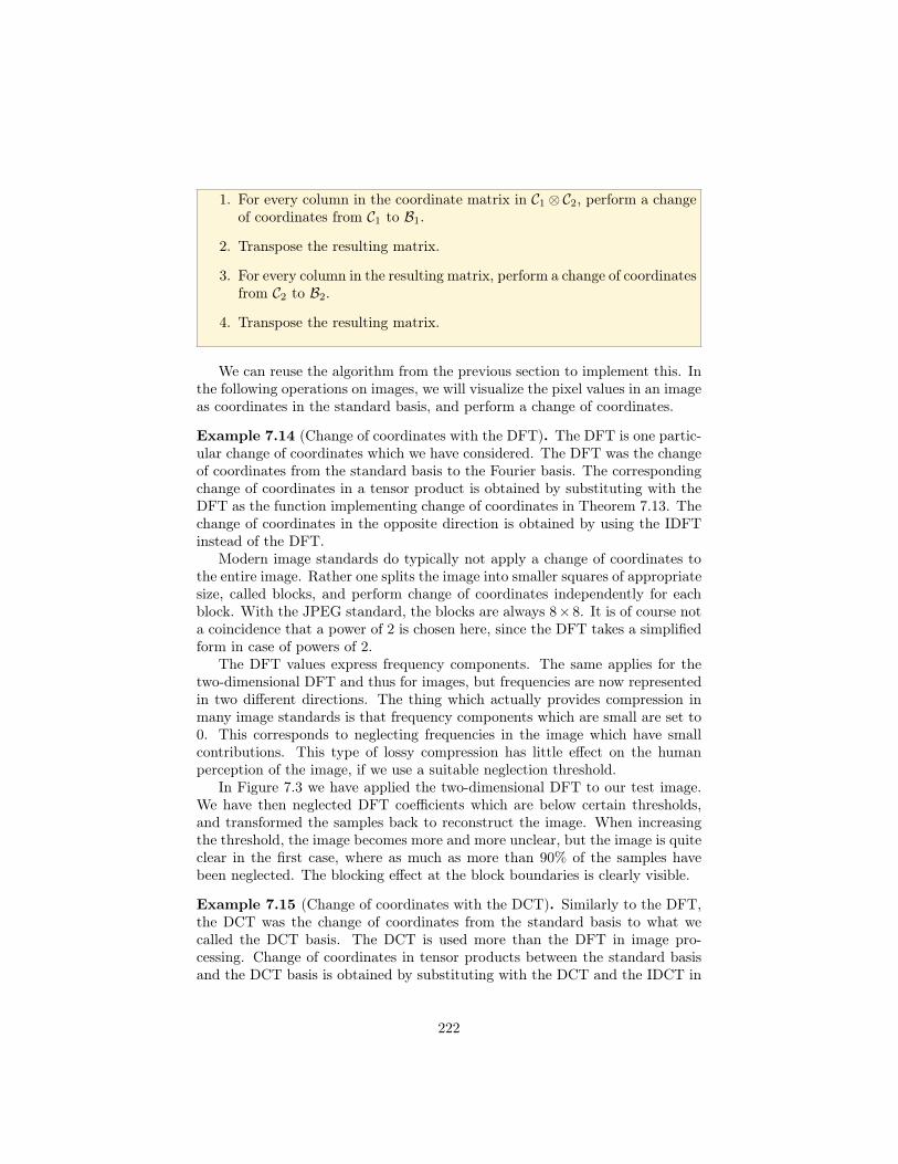
In Figure 7.3 we have applied the two-dimensional DFT to our test image.We have then neglected DFT coefficients which are below certain thresholds,and transformed the samples back to reconstruct the image. When increasingthe threshold, the image becomes more and more unclear, but the image is quiteclear in the first case, where as much as more than 90% of the samples havebeen neglected. The blocking effect at the block boundaries is clearly visible.

Example 7.15 (Change of coordinates with the DCT). Similarly to the DFT,the DCT was the change of coordinates from the standard basis to what wecalled the DCT basis. The DCT is used more than the DFT in image pro-cessing. Change of coordinates in tensor products between the standard basisand the DCT basis is obtained by substituting with the DCT and the IDCT in

222

(a) Threshold 30. 91.3%of the DFT-values were ne-glected

(b) Threshold 50. 94.9%of the DFT-values were ne-glected

(c) Threshold 100. 97.4%of the DFT-values were ne-glected

Figure 7.2: The effect on an image when it is transformed with the DFT, andthe DFT-coefficients below a certain threshold were neglected.

Theorem 7.13. The JPEG standard actually applies a two-dimensional DCT tothe blocks of size 8× 8, it does not apply the two-dimensional DFT.

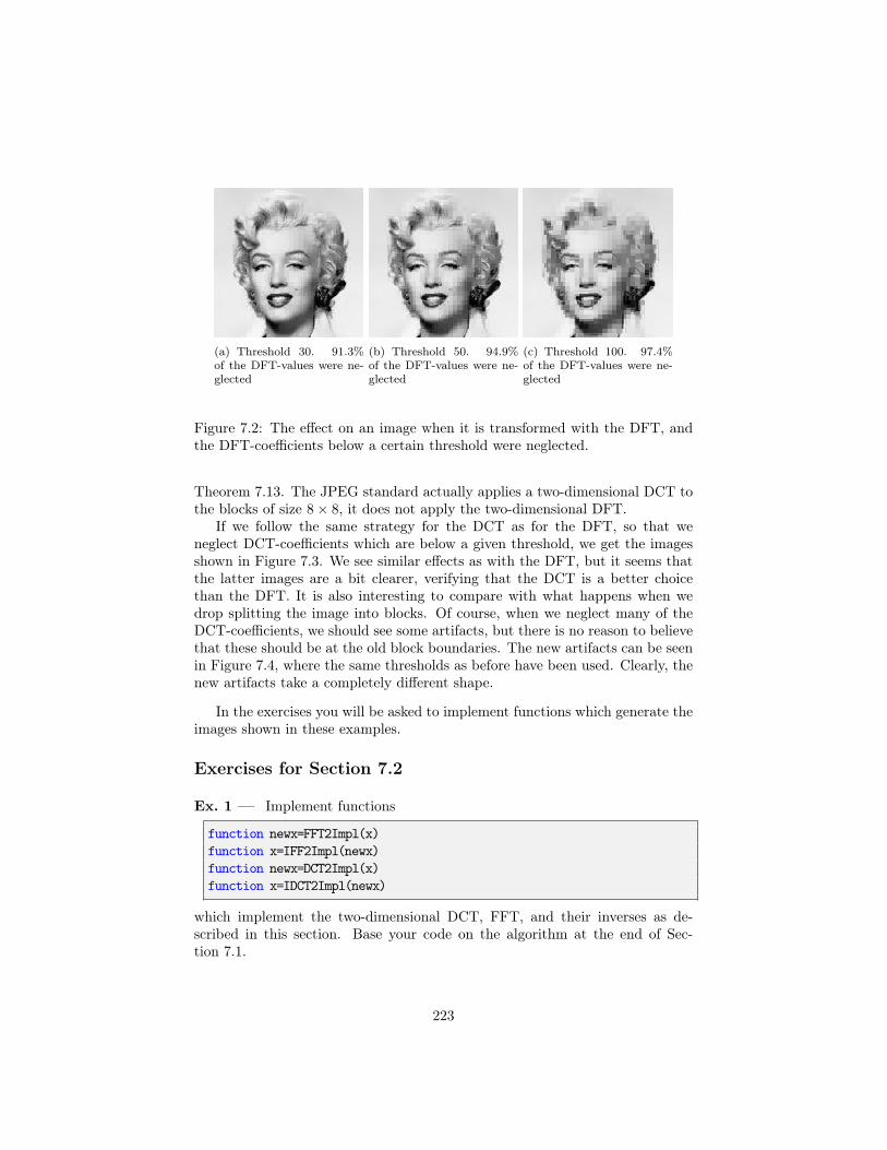
If we follow the same strategy for the DCT as for the DFT, so that weneglect DCT-coefficients which are below a given threshold, we get the imagesshown in Figure 7.3. We see similar effects as with the DFT, but it seems thatthe latter images are a bit clearer, verifying that the DCT is a better choicethan the DFT. It is also interesting to compare with what happens when wedrop splitting the image into blocks. Of course, when we neglect many of theDCT-coefficients, we should see some artifacts, but there is no reason to believethat these should be at the old block boundaries. The new artifacts can be seenin Figure 7.4, where the same thresholds as before have been used. Clearly, thenew artifacts take a completely different shape.

In the exercises you will be asked to implement functions which generate theimages shown in these examples.

Exercises for Section 7.2

Ex. 1 — Implement functions

function newx=FFT2Impl(x)function x=IFF2Impl(newx)function newx=DCT2Impl(x)function x=IDCT2Impl(newx)

which implement the two-dimensional DCT, FFT, and their inverses as de-scribed in this section. Base your code on the algorithm at the end of Sec-tion 7.1.

223

(a) Threshold 30. 93.9%of the DCT-values were ne-glected

(b) Threshold 50. 96.0%of the DCT-values were ne-glected

(c) Threshold 100. 97.6%of the DCT-values were ne-glected

Figure 7.3: The effect on an image when it is transformed with the DCT, andthe DCT-coefficients below a certain threshold were neglected.

(a) Threshold 30. 93.7%of the DCT-values were ne-glected

(b) Threshold 50. 96.7%of the DCT-values were ne-glected

(c) Threshold 100. 98.5%of the DCT-values were ne-glected

Figure 7.4: The effect on an image when it is transformed with the DCT, andthe DCT-coefficients below a certain threshold were neglected. The image hasnot been split into blocks here.

224

Ex. 2 — Implement functions

function samples=transform2jpeg(x)function samples=transform2invjpeg(x)

which splits the image into blocks of size 8×8, and performs the DCT2/IDCT2on each block. Finally run the code

function showDCThigher(threshold)img = double(imread(’mm.gif’,’gif’));newimg=transform2jpeg(img);thresholdmatr=(abs(newimg)>=threshold);zeroedout=size(img,1)*size(img,2)-sum(sum(thresholdmatr));newimg=transform2invjpeg(newimg.*thresholdmatr);imageview(abs(newimg));fprintf(’%i percent of samples zeroed out\n’,...

100*zeroedout/(size(img,1)*size(img,2)));

for different threshold parameters, and check that this reproduces the test im-ages of this section, and prints the correct numbers of values which have beenneglected (i.e. which are below the threshold) on screen.

7.3 SummaryWe defined the tensor product, and saw how this could be used to define op-erations on images in a similar way to how we defined operations on sound.It turned out that the tensor product construction could be used to constructsome of the operations on images we looked at in the previous chapter, whichnow could be factorized into first filtering the columns in the image, and thenfiltering the rows in the image. We went through an algorithm for computingthe tensor product, and established how we could perform change of coordi-nates in tensor products. This enables us to define two-dimensional extensionsof the DCT and the DFT and their inverses, and we used these extensions toexperiment on images.

225