DEGREE PREDICTION USING LOGISTIC REGRESSION

Faculty of Science Center of Mathematical Science Mathematical Statistics

DEGREE PREDICTION USING LOGISTIC REGRESSION

HAILEGEBRIEL KIDANEKAL AND ENDRIYAS ASSEFA

Master’s Thesis

Introduction .......................................................................................................................................1

CHAPTER 1

1 Related Study ................................................................................................................................3

CHAPTER 2

2 Data Description and Methodology ......................................................................................4

2.1 Data Description ………………………………………………………………………………………………………………..4

2.2 Logistic regression...................................................................................................................5

2.2.1Odds and odds ratio.........................................................................................................6

2.2.2 Logistic Regression Model……………………………………………………………………………………….6

2.2.3 Maximum likelihood Estimation of Logistic Regression Model…………………..7

2.3 Model Selection and Validation……………………………………………………………………………………10

2.3.1Akaike Information Criterion (AIC)………………………………………………………………………10

2.3.2 Significance Test for Model Estimates …………………………………………………………….10

2.4 Diagnosing Logistic Regression Models and Influential Observation……………..11

2.4.1 Pearson Residual…………………………………………………………………………………………………………11

2.4.2 Standardized Residual………………………………………………………………………………………………11

2.4.3 Deviance Residual …………………………………………………………………………………………………….11

2.4.4 Cook’s Distance …………………………………………………………………………………………………………12

2.4.5 DFBETAS ……………………………………………………………………………………………………………………….12

ii

CHAPTER 3

3 Data and Model Fit………………………………………………………………………………………………………………13

3.1 Model Fit …………………………………………………………………………………………………………………………….14

3.1.1 Model Diagnosis and Detecting Influential observation ………………………………20

3.1.2 Model for Students’ degree time at most 10 semesters ……………………………..23



CHAPTER 4

4 Model Prediction …………………………………………………………………………………………………………………29

CHAPTER 5

5 Conclusion ……………………………………………………………………………………………………………………………..39

5.1 Suggestion and Implication for Further Study …………………………………………………….40

References …………………………………………………………………………………………………………………………………41

ABSTRACT

To evaluate the efficiency of the previous years or to set visible plan in different

aspects for the upcoming years in higher institutions studying students’ time to

degree is important. Since logistic regression is a method used to predict a

dependent categorical outcome or predict the probability of an event occurrence,

studying Students’ time to degree using logistic regression is a reasonable way to

predict the probability of students’ time to graduate considering influential factors

that magnify and make a difference between different types of students. This

difference can be the difference between age, gender, study programmes and so on.

Thus, this study explores the prediction of degree at University of Lund Engineering

faculty students on time and in the consecutive semesters based on significant

factors.

1

Introduction

Lund University is one of the best and oldest universities in Sweden even in

Europe, it was founded in the year 1666. Through the past 348 years it contribute a

lot by producing educated and skilled man power to put the country in the top list of

developed countries in the word and this create sustainable development for

Sweden. Increasing skillful graduates has a great roll for healthy economy of the

country, so focusing on the rate of graduate is some how much related to the overall

development of the country. After each year’s graduation the university community

and administration evaluate their success, of course the students’ success because

graduate students are indicators of institutional quality and institutes are accountable

for lower rate of degree graduates.

Therefore, one of the quantifying measures will be how many of the students

who joined the university graduate on time each year. Answering this question helps

the university administration to see how successful it was in accepting new students

and produce skillful man power by the end of each year and also how successful it

was in spending budgets. Basically these three things which are accepting students,

graduating students and budget spending relate and affect each other, because

having students who do not complete their program on time puts more burden on

the next years plan and budget. Also the government supposes to know the

university budget as well as how many of the students need student allowance.

Since, in Sweden students takes credit money each month till they complete their

study. Consequently, the university administration expects the students to complete

their program on time and leave the place for the new students. Based on the above

reason and more other reasons that we don’t describe here the administration

needed to predict how many of the students will complete their program on time and

get their degree or what is the expectation of students proportion that graduate with

respect to time. These predictions are crucial to adjust the upcoming year plan

budget wise, accommodation and student funding money in case of government.

Accordingly, this thesis paper tries to identify the significant factors that really

matter to complete the program on time and in the following two consecutive

semesters then develops a model in order to make a prediction.

2

When we think about influential factors different kinds will come in our mind

such as economical, health condition, chance of getting job after school and others

but the data that we have for our study gives information only about factors related

to school activity. So our study will be limited on those factors that related to school

activities and somehow significant enough to describe students’ time to degree.

Thus, using this LTH student data we will try to follow logistic regression

methodology and fit logistic regression model that helps us to see which variables

are significant and make a difference on the probability of the students to complete

their program. After getting reasonable models that describe the variance the most

we will make prediction on students’ probability to graduate on time or one semester

later or a year later.

3

CHAPTER 1

1 Related Study

Before proceeding to our study let us revise a very related study written by

CHONNART PANYANGAM and KIA XIA (JUNE 2012) [7] which basically study time to

degree using Survival Analysis methodology on the same data set that we are about

to use for our study. It is better to preview summarized brief conclusion of the study,

they have tried to get reasonable survival function model to make a prediction which

contains variables that have impacts on students’ time to degree. The variables used

to fit the model are age, gender, admittance group, discontinuation of the program

in the middle of study, students who passed 60 credit hours or less during first year

and students who had more than or not more than two stop-out semesters.

Consequently, the fitted model was used to make prediction on six different types of

students’ sample groups, which are categorized by the variables that were used in

the model listed on the pervious statement.

In each variable perspective their study conclude that students who were forced

to enroll in a new program because the program that they enrolled for the first time

discontinued, will need more time than other students. Students who take more

stop-out semesters will graduate later and in gender wise female students will

graduate sooner than male students. Younger students have higher probability to

complete their study sooner than older ones. The study also concludes that students

who came from admittance group old gymnasium will graduate sooner than other

admittance groups. Finally, students who have tendency to cover more credit hours

in a year will graduate faster than those who can’t do so. Overall, according to this

study paper half of the students in a group, who had no more than two stop-out

semesters, got no less than 60 credit hours during first year, which are only between

17.5 and 21.5 years old, admitted from new gymnasium and which are female would

expect to graduate within 9 to 10 semesters. Additionally, two third of these students

get a degree by the 10th or 11th semester. Other types of student groups complete

their study programs one to two more semesters later compared to the previous

group and the time to graduate two third of them take 11th to 15th semester.

4

CHAPTER 2

2 Data Description And Methodology

2.1 Data Description

The most descriptive and effective studies success is choosing the right method

for the right data to analysis and made reasonable, reliable conclusions that lead to

efficient problem solving. This study is about students’ rate of graduation time to

degree based on influential factors that make students graduating time different

from one another which means on time or later than the standard time. Previously

we described the aim of the study, now let see the data description then we will

proceed to the methodology that will more adequate to reveal useful facts and get

reliable prediction result that fits the reality.

Here are the row data variables and their description

idnr Person identification number 1,. . . ,26 724

progr Education programme code

ppoang ECTS-credits for the programme

kaprogr Short code for programme groups

extyp Type of exam (A = architect, CI = civil engineer, HI = engineering bachelor)

examen terminated studes with exam (0 = no, 1 = yes)

nedl terminated studies because the programme was discontinued (0 = no, 1 = yes)

avbrott terminated programme without exam (0 = no, 1 = yes)

uhlang length, in semesters, of hiatus

uhall has had hiatus (0 = no (uhlang=0), 1 = yes (uhlang>0))

provp1 passed credits during first year

antalp1 number of passed tests during first year

kv gender (0 = man, 1 = woman)

ater admittance semester: 0,1,. . . ,43 = autumn 1988,. . . ,spring 2010

kter start of corresponding beginners

eter semester of exam or censoring

uter semester of first hiatus (missing = no hiatus)

ter2 semester when first started second semester of programme (ideally kter+1,

missing if no start on second semester)

ter3 semester when first started third semester of programme (ideally kter+2, missing

if no start on third semester)

ter5 semester when first started fifth semester of programme (ideally kter+4, missing

if no start on fifth semester) avter semester of termination of studies or censoring

age age (counted in semesters, 35 = 17.5 years) at kter

hak admitted to later part of programme (0 = no (kter=ater), 1 = yes (kter>ater))

kvgr admittance group (0 = old gymnasium, 1 = new gymnasium, 2 = national test,

3 = national test and work experience, 4 = foreign educ., 5 = folk high school,

6 = practical test, 7 = later part (hak=1), 8 = other

tid_ek time from kter to eter (exam or censoring)

5

tid_ea time from ater to eter (exam or censoring)

tidt2 time from second semester to eter (exam or censoring)

tidt3 time from third semester to eter (exam or censoring)

tidt5 time from fifth semester to eter (exam or censoring)

tid_eu time from ater to eter (exam or censoring), excluding time spent on hiatus

provp2 passed credits during second year

antalp2 number of passed tests during second year

provp3 passed credits during third year

antalp3 number of passed tests during third year

Note: at variable kvgr (admittance group) old Gymnasium refer for high school students who passed

through the grading system that was used before and including the year autumn 2003 and new

gymnasium refer for those who passed through the new grading system implemented starting from

autumn 2004.

From the list of variables and their description one can see that the data provide us

detailed information about the students from the admittance semester till they leave

the University. It described gender, admittance group, exam time, passed credit

hours and other school activities. Notice that the given students’ information depends

only on activities within the university; it does not include any other information

beyond that. May be there will be some factors which are direct consequences of

some other external factor but we only stick to what we are given.

From the data description above and the study direction we intend to do, it is

better to use either Survival analysis or Logistic regression methodologies because

Survival analysis is a method that involves modeling of time to event and the data

might be censored like the data we have. Since Survival analysis methodology

already has been used to predict graduation time of students we are going to use the

other alternative methodology which is Logistic regression because Logistic

regression is a method that involves predicting categorical dependent variable based

on continuous or/and categorical explanatory variables.

2.2 Logistic regression

Many educational research problems need statistical analysis of dichotomous type

of data. Many of these researches use logistic regression methodology to deal with

such kind of dichotomous dataset. Binary logistic regression is the method to explore

relation and influence between the dependent binary data and continues and/or

categorical independent variables.

6

2.2 .1 Odds and Odds Ratio

Odds are the ratio of probability of an event will occur divided by the probability of it

will not occur [8]. Mathematically

Odds=

=

where p is the probability of success

Odds always have values greater than zero and if odds value is larger than one it

means that success will occur more likely than failure. For example, odds= 4 means

we will observe four success for every one failure and if Odds= ¼ expect that the

reverse will occur. Odds ratio, as the name indicates, is the ratio of two Odds.

Mathematically Odds ratio =

Here, and refer to the probability of success in group 1 and group 2

respectively.

If the odds ratio value is greater than one it indicates that the odds of the

outcome in group 1 is larger than in group 2. Thus subjects in group 1 are more

likely to have success than subjects in group 2. If the odds is ratio less than the

value one, expect that the reverse will occur and if it equal to one subjects of odds of

both in group 1 and group 2 will equally likely occur. Logarithm of odds will show up

later so it is better to make clear here, as we have seen above Odds of an event lie

between 0 and positive infinity, notice that 1 is the base line for Odds so that the

Natural logarithm of Odds have no boundaries of domain they lie between negative

and positive infinity and 0 is the base line for natural logarithm of Odds.

2.2.2 Logistic Regression Model

Logistic regression model looks familiar especially to someone who is familiar

with linear regression, like standard regression it used a regression equation with

coefficients for all regressed variables but Logistic regression regress against the logit

of dependent variable, not the dependent variable itself [1]. Additionally, binary

logistic regression is a type of regression analysis where the dependent variable is a

7

dummy variable. The logistic regression model use logit transform and formula

represented as

(1)

Where = ( =1) =1 ( =0),

( =1), ( =0) is the probability of success and failure of an observation i

respectively.

= log-odds when all are 0

= increase in log-odds when is increased by one unit, j=1, …,

= increase in odds when is increased by one unit, j=1,…,

For the dependent variable coefficients in logit are the effects of the predictor on log

of odds.

2.2.3 Maximum Likelihood Estimation of Logistic Regression Model

The Logistics regression model coefficients tell us the relation between a

dummy dependent variable and continuous or/and categorical independent variables.

In logistic regression the coefficients estimates expect to have optimal values. This is

done with the maximum likelihood estimation method which helps to find the set of

parameters for which the probability of observed data is largest [5]. From equation 1

we can observe that each represents a binomial count in the population, the

maximum likelihood equation comes from the probability distribution of dependent

variable which is , the joint probability density function of is

Let us describe some of the notation; the combination function is the

number of different ways to arrange successes from trials that give as the

part

. For any one of these trials the probability of success is , similarly the

probability of failures is .The likelihood function is almost the

same as the probability density function except the parameters of the function are

reversed. Thus the likelihood function use fixed value for . So the function looks

8

(2)

Rearranging Eq.1 will give us

After solving for and using Eq.2 the equation to be maximized can be written as:

And taking the logarithm of both sides, the equation can be written as

After simplifying some steps we get

))

We take the derivative with respect to each and set equal to zero to get the

critical points of the log likelihood function

=…..= =0 (3)

The estimate for can be found by setting each of the k+1 equations at

equation 3 equal to zero and solve for each . This solution gives us a critical point

either a maximum or minimum and if the matrix of second partial derivatives is

negative definite it will be maximum [5].

9

This matrix also forms the variance-covariance matrix of the parameter estimates.

It can found by differentiating each of the k+1 equations in Eq.3 for the second time

with respect to each , so the form of the matrix of second partial derivative is

=

After using some general rules for differentiation we will get

(4)

Putting Eq.4 equal to zero results in k+1 nonlinear equations with k+1 unknown

variables. But solving a system of nonlinear equations is difficult, so that the solution

must be numerically estimated by using an iterative process. Accordingly we need to

apply Iterative solution using Newton-Raphson method. We want to find the roots for

Eq.3 simultaneously but it is better to use matrix notation. It is possible to write Eq.3

as and let represent a vector of initial approximations for each , the

initial step of Newton-Raphson can be expressed as

=

By using matrix multiplication we can see that

where is a column vector of length N with elements = and will be a

column vector of length k+1 with elements

. We also have

where W is a square matrix of order N with diagonal elements and

zero everywhere else, then , described using matrix multiplication as above ,is

a square matrix with elements

[5] . So we can write the initial

step Newton-Raphson as

= .

This iteration will continue until there is no change between the elements of

from one to the next iteration. Then the maximum likelihood estimates will converge.

For our study this computation done by R, which is programming language software

widely used among statisticians for data analysis.

10

2.3 Model Selection and Validation

Studies are mostly designed to answer certain questions, using methodology that is

most likely to model and answer those questions. In using Logistic regression model

one of the most challenging processes is selecting explanatory variables which

should be included in the model or not, even though sometimes the number of

variables is very large and make our study tougher to chose among the given

covariates. But our model should be complex enough to fit the data and easier to

interpret. So that, a search among models may provide clues about which predictors

are most associated with the response variable and suggest some questions for the

future study.

2.3.1 Akaike Information Criterion (AIC)

The Akaike Information Criterion [8] evaluates a model by how close to fitted

values to the true expected values. The optimal model is the one its fitted values

closest to the true outcome probabilities. The log likelihood of the model is the value

that is maximized by the process that computes the maximum likelihood value for

the coefficients which are parameters;

2.3.2 Significance Test for Model Estimates

Wald test: - The Wald test is defines as the ratio between the maximum likelihood

estimate divide by its standard deviation [2].

For large n, W approximate to normal distribution with mean zero and variance one.

Significance test against

If , we can reject at significance level .

11

2.4 Diagnosing Logistic Regression Models and Influential Observation

2.4.1 Pearson Residual

Each Pearson residual is the difference between an observed count and its

expected value divided by the estimated binomial standard deviation of the expected

count [2].

Let denote the number of “successes” for trials at setting of explanatory

variables and is the estimated probability of successes for the model fit. Which

is estimated binomial mean is the fitted number of successes. It uses to test lack of

model fit.

(i.e. Bin (1, with ))

2.4.2 Standardized Residual

Because of the binary nature of the dependent variable analyzing residual in

logistic regression is not direct forward. The other type of residual that diagnoses the

model fit is Standardized residual.

Standardized residual=

Here is the observation’s leverage its elements come from the matrix

that yields the predicted logit values for the model. The larger the

greater its potential influence on the model fit [2]. So as we have seen from the above it is larger in absolute value than the Pearson residual.

2.4.3 Deviance Residual An alternative residual based on the deviance or likelihood ratio chi-squared statistics is the deviance residual and it defined as [2]

=

Squaring these residuals and summing over all observations yields the deviance

statistics. Observations with a deviance residual in excess of two may indicate lack of

fit.

12

2.4.4 Cook’s Distance

The most common summary measure of influential point is Cook’s distance which

is just a weighted sum of squares of the difference between each element of the

coefficient vectors. Interestingly, it can be computed from diagnostic statistics that

we have already encountered [1]

If we can say the observation is influential point on

the model.

2.4.5 DFBETAS

DFBETA use to measure the influence of the observation is defined as the

one-step to the difference in the MLE of the parameter vector and the MLE of the

parameter vector without observation. This one-step assumes a Fisher scoring

step, and is given by

Where is the leverage and is the standardized Pearson residual

DFBETAS is the standardized DFBETA statistics for assessing the influence of

observation on the regression parameter is defined as DFBETA for the

parameter divided by its estimated standard deviation, here the standard deviation is

estimated from the data.

=

Values of greater than two would certainly indicate a major impact

from a single point [3].

13

CHAPTER 3

3 Data and Model Fit

As described in the introduction part this thesis is a study about the prediction of

student time to degree. When we write about students’ time to degree it is basic to

know influential factors that have impacts on raising or declining the probability of

students’ to graduate directly or indirectly. Sometimes factors which are influential to

graduate on time may not be influential to graduate late. So, we will go further to

see those consistent variables on the consecutive semesters. We are going to use

the history data of LTH students who were admitted at Lund University from autumn

1988 to spring 2010. Our dataset has 29,163 with 34 different variable values but we

can’t use this row data directly. Rather, it needs some adjustment before applying

the logistic regression methodology to analysis and get reasonable results. As we can

see in the data description in chapter 2 shows list of variables that describes

students’ activity in the University.

As we look through the 29163 data set there are NA (not available) values in the

dependent variable so remove these values from the data, for our study analysis

select exam type for only Civil engineer students who must take 270 credit hours for

entire program. After this adjustment we only use the total of 14,317 observations

for modeling purpose. We also save adjusted data for prediction and make similar

adjustment. So what we have done is we took the data starting from year 1988-2006

for modeling and the rest starting from 2007 to the end which is spring 2010

semester for prediction and analysis.

Before applying the chosen methodology, which is logistic regression, let us go

through our adjusted modeling data in simple descriptive statistical measures it

might help for better understanding of the data structure.

The observed students have ages between 18 and 55 years old and about one

third of them are female. Majority of these students were admitted from two groups,

which are new and old Gymnasiums they take 25.57% and 31.96% of the total

revised observed data respectively. Regardless of analyzing the dataset number of

credit hours passed during each year stay does matter to complete their program on

time, so let us see the rough structure of passed credit hours at least for three years

stay at the university. Out of 14317 students only 2734, 3815 and 4102 students

passed at least sixty credit hours during first, second and third years study

respectively.

14

As we have seen the sequence the number of students who passed at least sixty

credit hours in each year increases when we observe their stay from first to third

year. Additionally, only 766 of them passed at least sixty credit hours and 676 of

students couldn’t pass any credit hours consistently for consecutive three years

which are from first year to third year of their stay respectively.

Gender wise the proportion of the students who passed at least sixty credit

hours for the consecutive three years are almost similar but males have larger

proportion than females. If we take look on the event that on taking a break in the

middle of the study, around 66.68% of the students do not take any break at all.

Surprisingly, out of 676 who couldn’t pass any credit hours from the first to third

year 528 of them do not take any break. Women have slightly larger proportion in

taking a break out in semester than men which is about 38.8% for female and

31.5% for male students. In terms of age out of 10778 who are at least 21.5 years

old about 3833 of them take a break which shows higher proportion than the

students who have older age group which is older than 21.5 years. It seems that

older men who are older than 21.5 years have larger proportion in the data than

female students with the similar age category.

variables Categories in each variables Number of students in each category

Total number of students

Age Age 43 semesters (21.5 years) 10778 14317

Age 44 semesters (22 years) 3539

Kv (gender) 0 (Male) 10773 14317

1 (Female) 3544

Uhall (break)

0 (no breaks) 9547 14317

1 (takes break) 4770

Kvgr (admittance group)

0 (old gymnasium) 3661 14317

1 (new gymnasium) 4576

2 (national test) 1451

3 (national test and work experience) 2117

Others (4,5,6,7 and 8) 2512

Table 1 number of students in three categorical variables, uhall (break), kvgr

(admittance group), kv (gender) and in two age category groups.

15

3.1 Model Fit

After we revised our dataset it contains 14317 observations whose credit hours is

270 for entire program which are only civil engineering (extype=CI). Since these

students need 9 semesters or four and half years to complete their degree program

on time then we need to take students who admitted before and including spring

semester 2006 ( ) for modeling and the later admitted ones for prediction.

To get the best model one of the most essential processes is deciding which

variables should or shouldn’t be included in the model especially when we have many

variables similar to our case, too many variables bring too many choices.

We are going to use Logistic regression methodology to analyze the historic LTH

student data. Using two variables which are and we make the

dependent variable named , for equal to

one otherwise zero. After creating dependent variable, even though having many

variables make our model selection hard enough but we try to eliminate some

variables because of collinearity and significance in the model.

Let us see some of the collinear variables, from the revised data and

are correlated to each other, since these all three variables give us information

about whether students take a break in the semester or not. , and

are also collinear with one another. Similarly, are among the

variables that are collinear, since both provide us information about students’ status

based on termination of studies with exam or not.

Because of multi collinearity we eliminate some of the variables and try to fit

logistic regression model including most interesting variables. Remember that our

dependent variable is which is equal to one if

otherwise zero. Stepwise method helps us to select which variables we need to

include in the model and which are not. This method detects significance of a

variable and eliminates variables if they are not significant. The elimination will

continue until all variables in the model are significant. Even though Akaike’s

Information Criterion (AIC) is biased for large number of parameters to choose best

model between models we use it with combing ANOVA table and make a decision to

select the best model that describe the dependent variable the most.

Finally we get a reasonable logistic regression model using only eight independent

variables, which are , , , , , , and

with the dependent variable called . But before getting the estimates we need

to summarize two of our variables which have so many sub-groups. These variables

are and , the descriptions of these two variables are is

admittance group and is short code for program groups.

16

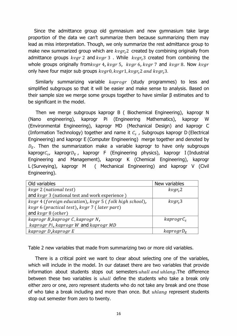
Since the admittance group old gymnasium and new gymnasium take large

proportion of the data we can’t summarize them because summarizing them may

lead as miss interpretation. Though, we only summarize the rest admittance group to

make new summarized group which are created by combining originally from

admittance groups and . While created from combining the

whole groups originally from , , , and . Now

only have four major sub groups

Similarly summarizing variable (study programmes) to less and

simplified subgroups so that it will be easier and make sense to analysis. Based on

their sample size we merge some groups together to have similar β estimates and to

be significant in the model.

Then we merge subgroups kaprogr B ( Biochemical Engineering), kaprogr N

(Nano engineering), kaprogr Pi (Engineering Mathematics), kaprogr W

(Environmental Engineering), kaprogr MD (Mechanical Design) and kaprogr C

(Information Technology) together and name it , Subgroups kaprogr D (Electrical

Engineering) and kaprogr E (Computer Engineering) merge together and denoted by

. Then the summarization make a variable kaprogr to have only subgroups

kaprogr , kaprogr , kaprogr F (Engineering physics), kaprogr I (Industrial

Engineering and Management), kaprogr K (Chemical Engineering), kaprogr

L (Surveying), kaprogr M ( Mechanical Engineering) and kaprogr V (Civil

Engineering).

Old variables New variables and

, , , and

, ,

, and

,

Table 2 new variables that made from summarizing two or more old variables.

There is a critical point we want to clear about selecting one of the variables,

which will include in the model. In our dataset there are two variables that provide

information about students stops out semesters .The difference

between these two variables is define the students who take a break only

either zero or one, zero represent students who do not take any break and one those

of who take a break including and more than once. But represent students

stop out semester from zero to twenty.

17

Unlike variable summarize the wide range only in to zero and one.

Since, the above model is to see the students to degree on 9 semesters which means

on time within four and half years the variable is not significant for our model

at this level.

Even though, it give us more information than and we even try to

summarize the wide range of to three main sections but still it is not

significant enough in the model. Therefore, is an appropriate variable for the

model in case of students stop out semester information to model for students who

complete their study on time which is four and half years.

After we go through all the adjustment, summarization and analyzing interesting

variables finally time to reveal our best model and its estimates. To compute the

logistic model fits we use R which is widely used among statisticians for data

analysis. The table below is the model estimates on time for students who need to

take 270 credit hours for the entire programme and we named it Model 9.

Log odd ratio Estimates

Odds ratio

95 % Confidence Interval Odds ratio

Pr(>|z|)

2.5% 97.5 %

Intercept -8.48 0.00 0.00 0.00 < 2e-16 *** 0.06 1.06 1.05 1.07 < 2e-16 ***

0.05 1.05 1.04 1.05 < 2e-16 *** 0.03 1.03 1.03 1.04 < 2e-16 *** 0.02 1.02 1.02 1.02 < 2e-16 *** 0 1 - - - -2.17 0.11 0.09 0.15 < 2e-16 ***

0 1 - - -

0 -1.34 0.26 0.22 0.31 < 2e-16 ***

1 -1.64 0.19 0.16 0.23 < 2e-16 ***

-1.60 0.20 0.17 0.24 < 2e-16 *** 0 1 - - -

0.38 1.46 1.26 1.69 6.00e-07 *** 0 1 - - - 0.36 1.43 1.10 1.86 0.008597 ** 0.20 1.22 0.98 1.52 0.083495. 0.81 2.24 1.66 3.02 1.39e-07 *** 0.48 1.61 1.24 2.10 0.000424 *** 0.72 2.06 1.49 2.84 1.14e-05 *** 0.34 1.38 1.08 1.75 0.009406 ** 0.56 1.75 1.35 2.26 2.60e-05 ***

Table 3 Logistic regression model estimates of Model 9 in terms of log odds ratio , odds

ratio , 95% confidence interval for Odds ratio and 95% significance level of each variable for

the students who graduate at most 9 semesters time.

18

Significant codes: 0 ‘***’ 0.001’ **’ 0.01’ *’ 0.05 ‘0.1’ ‘ ’ 1

Null deviance: 10121.7 on 14316 degrees of freedom

Residual deviance: 6897.2 on 14300 degrees of freedom

AIC: 6931.2

Df Deviance Resid.Df Resid.Dev Pr(>Chi)

NULL 14316 10121.7

Age 1 22.00 14315 10099.7 2.733e-06 ***

Provp1 1 1425.86 14314 8673.9 < 2.2e-16 ***

Provp2 1 592.25 14313 8081.6 < 2.2e-16 ***

Provp3 1 245.01 14312 7836.6 < 2.2e-16 ***

as.factor(kvgr), ref = "3" 3 483.31 14309 7353.3 < 2.2e-16 ***

kaprogr, ref = "F" 7 51.64 14302 7301.7 6.875e-09***

as.factor(uhall) 1 379.94 14301 6921.7 < 2.2e-16***

Kv 1 24.55 14300 6897.2 7.235e-07***

Table 4, ANOVA table for logistic regression model estimates shown in Table 3

, i=1,2……..14,317.

The reference group of covariates for each category , , and

are , , and .

As shown in the table 4 all main eight variables are significant at 5% significance

level with model AIC value 6941.50. One can notice that on Table 3 has

slightly significant reference to program group F; this means that the program

group almost has similar probability with group F to graduate within nine

semester time which is the program group as reference group to estimate the model

parameters on time to degree.

There are some observations that have extreme values, specifically for variable

which is a student passed credit for the first year. Five students passed over

100 credit hours for their first year stay; of course we worried that these values may

affect the estimates and try to fit the model with and without these extreme values.

19

Regardless of these values the model estimates stay constant so it is not necessary

to remove these values. In the residual analysis part we will see if this decision

brings any model inadequacy.

Our computed coefficients for the logistic regression model which, are seen in

Table 3 are estimated increase or decrease of log odds for students who graduate on

time for each variable in one unit increase. The coefficient for age indicates that a

one semester increase of the age of a student increases the odds of graduating on

time by 1.06. Similarly, passing a credit hour increase odds of graduating on time by

1.05, 1.03 and 1.02 from the first to third year respectively, which means students

who passed certain credit hours on the first year have higher probability to graduate

relative to students who passed the same credit hours on the second or third year.

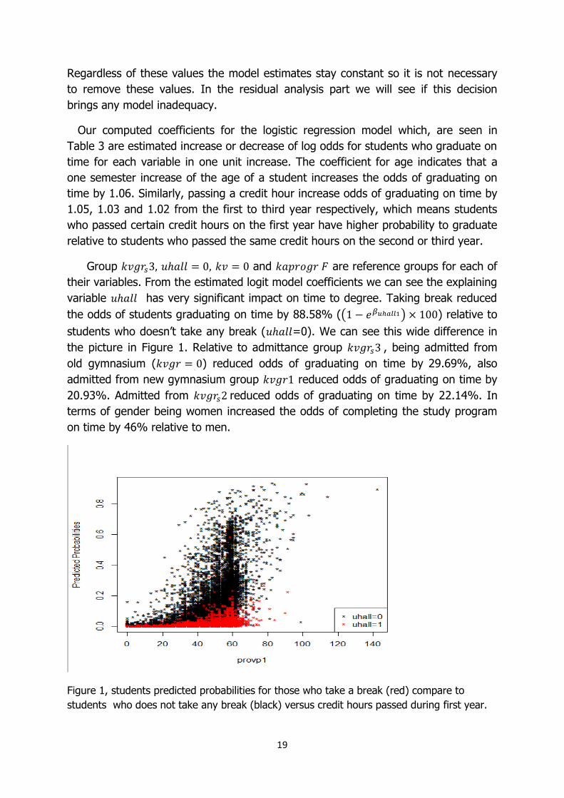
Group and are reference groups for each of

their variables. From the estimated logit model coefficients we can see the explaining

variable has very significant impact on time to degree. Taking break reduced

the odds of students graduating on time by 88.58% ( ) relative to

students who doesn’t take any break ( =0). We can see this wide difference in

the picture in Figure 1. Relative to admittance group , being admitted from

old gymnasium ( ) reduced odds of graduating on time by 29.69%, also

admitted from new gymnasium group reduced odds of graduating on time by

20.93%. Admitted from reduced odds of graduating on time by 22.14%. In

terms of gender being women increased the odds of completing the study program

on time by 46% relative to men.

Figure 1, students predicted probabilities for those who take a break (red) compare to

students who does not take any break (black) versus credit hours passed during first year.

20

3.1.1 Model Diagnosis and Detecting Influential Observation

After a model has been fit, it is wise to check the model to see how well it fits the

data. By computing different types of residuals which are Pearson’s residual,

Deviance residual, Standardized residual and plotting these residuals help us to judge

the model fit. Cook’s distance helps us to identify influential points. Diagnostic plots

for Model 9 are show below which models student’s time to degree within nine

semester’s time that is on time for 270 credit hours students.

Figure 2, Diagnostic plots for the model fit to predict student’s time to degree at most 9

semesters (Model 9).

21

For checking the systematic part of models, plots of the residuals against the

predicted probability values. Figure 2 (top left) shows Pearson residuals and Figure 2

(bottom left) shows deviance residuals. These residual plots show an obvious pattern

on one curve above and one curve below the line zero. This is because of the binary

outcome, nothing to do with bad model fit. For acceptable fit one would expect that

locally the residual average zero, the smooth line helps in detecting a deviation from

this expectation. Therefore, overall from these residual plots our model fit is very

acceptable.

In Figure 2 (top right) the shape of the plot show quadratic curves. If our model

fit poorly we may see points falling in the top left or top right. Assessment of the

distance is partly numerical values and partly visual impression. On bottom right of

Figure 2 the Cook’s distance plot shows us there are no observation that has major

influence on the model estimates.

Hence, it can be concluded that no significant model inadequacy and presence of

influential outliers are observed in the covariates space. Thus, the existing outliers

detected by residual plots are not influential. We should see the efficiency of our

model using our modeling data and one can judge how good the model is and see

how much of our independent variables describe our dependent variable which is the

students time to graduate within nine semester it counts four and half years.

22

Figure 3, DFBETAS index plots of six variables of the model that used to fit the students time

to degree for nine semesters.

Figure 3 helps us to detect influential observations that affect the model

estimates. According to the figure except the estimate for variable there are no

major influential observations that influence on model estimates. Interestingly, in

case of variable there are observations that depart from the majority

observations, this two depart cluster of observations tell us there are a few

observations who might have slight influence on the model estimate that involve with

students taking a break in the middle of the study programme.

23

3.1.2 Model for students’ degree time at most 10 semesters

For students’ time to degree in at most 10 semesters’ time, to model the logodds

of students who complete their study within 10 or less semesters we need to adjust

the data a little more as follows. It is important to adjust the admittance semester so

we take students who were admitted before and including autumn semester 2005

( for modeling data for 10 semesters’ time. Then we fit the binary logistic

regression model and we found the following estimates. The model below is one

semester later for 270 credit hours major students but on time for 300 credit hours

major students, since for 300 credit hours major students 10 semester time is the

standard time and to identify this model from the other models named it Model 10.


Odds ratio 95 % Confidence Interval Odds Pr(>|z|)

2.5% 97.5%

Intercept -8.85 0.00 0.00 0.00 < 2e-16 *** 0.04 1.04 1.03 1.06 < 2e-16 ***

0.06 1.05 1.05 1.06 < 2e-16 *** 0.04 1.04 1.04 1.05 < 2e-16 *** 0.03 1.03 1.03 1.04 < 2e-16 ***

0 1 - - - -1.99 0.14 0.12 0.16 < 2e-16 ***

0 1 - - -

0 -1.09 0.34 0.29 0.40 < 2e-16 ***

1 -1.03 0.36 0.30 0.42 < 2e-16 *** -1.20 0.30 0.26 0.36 < 2e-16 ***

0 1 - - - 0.37 1.44 1.27 1.63 1.18e-08 ***

0 1 - - - 0.50 1.66 1.33 2.07 8.98e-06 *** 0.44 1.55 1.29 1.88 4.81e-06 *** 0.98 2.65 2.03 3.48 1.19e-12 *** 1.00 2.73 2.18 3.42 < 2e-16 *** 0.70 2.00 1.51 2.66 1.36e-06 *** 0.87 2.39 1.95 2.93 < 2e-16 *** 1.04 2.82 2.25 3.52 < 2e-16 ***

Table 5 Logistic regression model estimates of Model 10 in terms of log odds ratio, odds

ratio, 95% confidence interval for Odds ratio and 95% significance level of each variable for

the students who graduate in at most 10 semesters.

Significant codes: 0 ‘***’ 0.001’ **’ 0.01’ *’ 0.05 ‘0.1’ ‘ ’ 1



AIC: 9126.3

24


NULL 1 14288 16719.8

Age 1 5.4 14287 16714.4 0.01982 *

Provp1 1 3277.4 14286 13437.0 < 2.2e-16 ***

Provp2 1 1773.8 14285 11663.2 < 2.2e-16 ***

Provp3 1 1377.5 14284 10285.6 < 2.2e-16 ***


kaprogr, ref = "F" 1 711.4 14280 9300.8 < 2.2e-16 ***

as.factor(uhall) 7 175.8 14273 9125.0 < 2.2e-16 ***

Kv 1 32.7 14272 9092.3 1.093e-08***

Table 6, ANOVA table for logistic regression model estimates shown in Table 5 (Model 10).

From Table 6 we can see the variables in the Model 10 are significant at 5% significance

level.

Residual plots for the model that fit students who complete their study at most 10

semesters (Model 10) shown below

Figure 4 Diagnostic plots for the model fit to predict student’s time to degree at most 10

semesters (model 10). The interpretation of the figure is similar to Model 9 diagnostic plot

(section 3.1.1).

25


For students’ time to degree at most 11 semesters time, to fit the logistic

regression model for students who complete their programme for 11 semesters we

need a little more adjustment to model. Here we need to substitute variable by

variable because has a wider range than . The amount of break

can possibly influence for the students who complete their study for two or more

semesters late. Additionally, the admittance semester must be before and including

spring semester 2005 for modeling data. See the estimates in Table 7

below. The model below is a model a year later for 270 major credit hours but one

semester later for students whose major is 300 credit hours and to identify this

model from the others we call this model Model 11.


Odds ratio

95 % Confidence Interval Odds Pr(>|z|)

2.5% 97.5%

Intercept -7.24 0.00 0.00 0.00 < 2e-16 *** 0.02 1.02 1.01 1.03 0.000109 ***

0.05 1.05 1.05 1.06 < 2e-16 *** 0.04 1.04 1.04 1.05 < 2e-16 *** 0.03 1.03 1.03 1.04 < 2e-16 *** 0 1 - - - -0.97 0.38 0.33 0.43 < 2e-16 ***

2 -4.68 0.01 0.00 0.03 1.82e-15 *** 0 1 - - -

0 -0.69 0.50 0.43 0.59 < 2e-16 *** -0.87 0.42 0.36 0.50 < 2e-16 *** -0.97 0.38 0.32 0.45 < 2e-16 ***

0 1 - - - 0.34 1.40 1.24 1.59 1.53e-07 ***

0 1 - - - 0.12 1.13 0.91 1.42 0.278616 0.31 1.36 1.13 1.64 0.001298 ** 0.62 1.86 1.41 2.45 9.40e-06 *** 0.54 1.72 1.38 2.15 1.73e-06 *** 0.34 1.40 1.05 1.88 0.022467 * 0.63 1.88 1.54 2.31 1.24e-09 *** 0.81 2.25 1.80 2.82 1.87e-12 ***

Table 7 Logistic regression model estimates of Model 11 in terms of log odds ratio, odds

ratio, 95% confidence interval for Odds ratio and 95% significance level of each variable for

the students who graduate at most 11 semesters time.

Null deviance: 17234 on 13202 degrees of freedom

Residual deviance: 9040 on 13185 degrees of freedom

AIC: 9076

26


NULL 13202 17234.4

Age 1 55.5 13201 17178.9 9.415e-14***

Provp1 1 3807.3 13200 13371.6 < 2.2e-16 ***

Provp2 1 2211.3 13199 11160.3 < 2.2e-16 ***

Provp3 1 1385.5 13198 9774.7 < 2.2e-16 ***


as.factor(uhlang) 2 433.2 13193 9159.7 < 2.2e-16 ***

kaprogr, ref = "F" 7 92.0 13186 9067.7 < 2.2e-16 ***

Kv 1 27.7 13185 9040.0 1.388e-07***

Table 8, ANOVA table for logistic regression model estimates shown in Table 7 (Model 11).

Table 8 shows us the variables in the Model 11 are significant at 5% significance level.

Residual plots for the model that fit students who complete their study at most 11



semesters (Model 11). The interpretation of the figure is similar to Model 9 diagnostic plot

(section 3.1.1).

27


For students’ time to degree at most 12 semesters time, to fit the logistic

regression model for students who complete their program within at most 12

semesters’ time still need to keep variable rather than since

has wider range than because still the amount of break that students take in

the middle of the study program has influence for the students who complete their

study late. Interestingly, age is not significant any more for the students who

complete their study at most twelve semesters’ time, so we exclude the age variable

from the model. Additionally, the admittance semester must be before and including

autumn semester 2004 for modeling data.


Odds ratio

95 % Confidence Interval Odds Pr(>|z|)

2.5% 97.5%

Intercept -5.85 0.00 0.00 0.00 < 2e-16 ***

0.05 1.05 1.05 1.06 < 2e-16 *** 0.04 1.04 1.04 1.05 < 2e-16 *** 0.03 1.03 1.03 1.04 < 2e-16 *** 0 1 - - - 0.19 1.21 1.07 1.38 0.00222 **

2 -2.97 0.05 0.03 0.08 < 2e-16 ***

0 1 - - -

0 -0.42 0.66 0.56 0.77 5.09e-07 ***

-0.63 0.53 0.45 0.63 1.76e-14 *** -0.81 0.44 0.37 0.53 < 2e-16 *** 0 1 - - - 0.47 1.59 1.40 1.82 2.05e-12 ***

0 1 - - - -0.24 0.79 0.64 0.96 0.01732 * -0.25 0.78 0.65 0.95 0.01096 * 0.42 1.53 1.19 1.99 0.00121 ** 0.41 1.51 1.24 1.84 4.10e-05 *** -0.43 0.65 0.50 0.85 0.00178 ** 0.49 1.63 1.39 1.92 1.92e-09 *** 0.50 1.64 1.36 1.98 3.01e-07 ***

Table 9 Logistic regression model estimates of Model 12 in terms of log odds, odds, 95%

confidence interval for Odds and 95% significance level of each variable for the students

who graduate at most 12 semesters time.



AIC: 8900.9


28

NULL 13151 18150.2

Provp1 1 4869.6 13150 13280.6 < 2.2e-16 ***

Provp2 1 2623.2 13149 10657.4 < 2.2e-16 ***

Provp3 1 1189.6 13148 9467.8 < 2.2e-16 ***


as.factor(uhlang) 2 298.2 13143 9057.8 < 2.2e-16 ***

kaprogr, ref = "D" 7 140.6 13136 8917.2 < 2.2e-16 ***

Kv 1 50.3 13135 8866.9 1.345e-12 ***

Table 10, ANOVA table for logistic regression model estimates shown in Table 9.

Table 10 shows us the variables in the Model 12 are significant at 5% significance level.

Residual plots for the model that fit to students who complete their study at most 12



semesters (Model 12). The interpretation of the figure is similar to Model 9 diagnostic plot

(section 3.1.1).

29

CHAPTER 4

4 Model Prediction

In the previous chapter we developed a model using variables which have high

significant impact on the degree time of the student and we saw that it fits well

enough to the data. In this part of the study we are going to use our model to

predict the probability of the students to complete their program study on time. At

the same time we will try to analyze the output. Here the prediction will help us to

evaluate how reasonable the output of our model is relative to the real condition of

the students.

So the prediction is made on a different dataset other than the modeling dataset.

Since students who were admitted before and including spring semester 2006

used as modeling dataset now we are going to take students who were

admitted after this semester ( ). But in this data we have students with 270

credit hour and others with 300 credit hours. It is because LTH has increased the

major credit hours from 270 to 300 in the year 2007. Then for our prediction purpose

we choose students with the new credit hours that means those who needs a total of

300 credit hours to graduate and get a degree. This makes the total number of the

prediction data become 1081. Since we have eight main variables in the model and

even more, there are variables that have subgroups, so it will be quite a lot to make

a prediction and analyze for each individual student. Instead we decided to form a

group of students according to the variables we have in the model. The combination

of different variables to form different types of student groups is also too many but

what we are going to do is that we will take four of the variables and make a

combination to form interestingly different types of student groups. The grouping is

done with variables age, uhall/uhlang, kv, kvgr. Age is divided in to two groups one

less or equal 43 semesters age ( 21.5 years old) , the other ones are age greater

than 43 semesters age (i.e. starting from 22 years old), with this age division male

and female are categorized with whether they take a break or not including the

admittance group they came from. This gives us 16 different groups. Thus after

forming this group we further select out those groups of students who have better

advantage to get their degree on time and those who are relatively less likely to get

their degree on time, based on the model estimate values . For instance, women

have better chance than men in case of gender category, so according to our model

women who don’t take any break are most likely have a better chance than men who

take a break and so on.

30

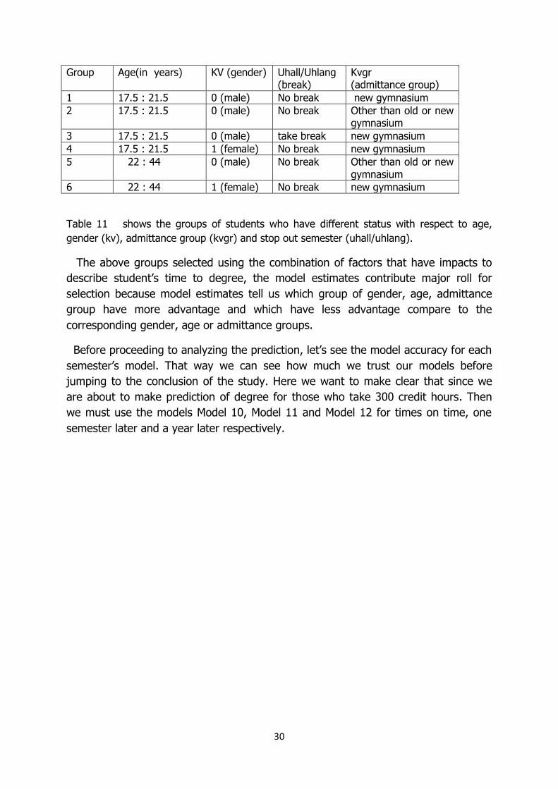
Group Age(in years) KV (gender) Uhall/Uhlang (break)

Kvgr (admittance group)

1 17.5 : 21.5 0 (male) No break new gymnasium

2 17.5 : 21.5 0 (male) No break Other than old or new gymnasium

3 17.5 : 21.5 0 (male) take break new gymnasium

4 17.5 : 21.5 1 (female) No break new gymnasium

5 22 : 44 0 (male) No break Other than old or new gymnasium

6 22 : 44 1 (female) No break new gymnasium

Table 11 shows the groups of students who have different status with respect to age,

gender (kv), admittance group (kvgr) and stop out semester (uhall/uhlang).

The above groups selected using the combination of factors that have impacts to

describe student’s time to degree, the model estimates contribute major roll for

selection because model estimates tell us which group of gender, age, admittance

group have more advantage and which have less advantage compare to the

corresponding gender, age or admittance groups.

Before proceeding to analyzing the prediction, let’s see the model accuracy for each

semester’s model. That way we can see how much we trust our models before

jumping to the conclusion of the study. Here we want to make clear that since we

are about to make prediction of degree for those who take 300 credit hours. Then

we must use the models Model 10, Model 11 and Model 12 for times on time, one

semester later and a year later respectively.

31

Model accuracy table

Table 12, model prediction accuracy table for models Model 10, Model 11 and Model 12

that fits for students who at most need 10, 11 and 12 semesters to graduate

respectively.

From the above table it is clear that all our models have around 85% over all

model accuracy which indicates that the model covariates well describe the

variance of the dependent variable. Using these best accurate models we make

prediction for student’s probabilities for the described groups of students and

see which groups of students have better chance to get their degree on time or

within 11 semesters or 12 semesters.

Group Predicted probabilities for 10 semesters (on time)

Predicted probabilities for 11 semesters ( one semester later)

Predicted probabilities for 12 semesters (a year later)

1 37.23% 51.42% 59.58%

2 34.97% 42.62% 48.09%

3 - 12.63% 28.42%

4 66.42% 72.39% 77.61%

5 31.18% 43.02% 46.24%

6 54.84% 61.29% 67.74%

Table 13, Predicted probabilities of students’ for different type of groups to complete

their study on time, one semester later and one year later.

10 semesters (Model 10)

Predicted category

Correctly classified

Number of observation

Observed category

1 0

3884 1 2620 1264 67.46%

10405 0 287 10118 97.24%

Over all accuracy 89.17%



4736 1 3878 858 81.88%

8467 0 1191 7276 85.93%




6056 1 5309 747 87.67%

7096 0 1278 5818 81.99%


32

Let us analyze the predicted probabilities shown in table 13, since we are

studying students’ time to degree notice that the amount of students that

graduate increase from ten semesters time to one year later time regardless of

the groups they belong to. Group 3 contains the least likely type of students to

graduate according to our table; these students are male students who took

break and admitted from new gymnasium. Here one of the most influential factor

is taking a break because irrespective of the other factors a student that has to

study 300 credits hours for the entire programme it means the student standard

time to complete the study need 10 semesters but if a student takes a break in

the middle of the five year programme most likely such kind of students need

more time to get their degree that is why the probability for students from group

3 is very low relative to the others.

The probabilities for male and female students with the same other covariate

categories that are used for grouping are shown in group 1 and group 4

respectively. Two third of female students who do not take a break and are

admitted from new gymnasium would graduate on time, about more than seventy

five percent of these female students expected to graduate at most a year later

than the standard time. In case of group 1 which contains male students of the

same category unlike female students, about one third of students from group 1

would graduate at most one semester later.

33

Figure 7, Predicted probabilities of students to get a degree at most 10 semesters who

belong to Group 1 (17.5: 21.5 years old, male, no break and new gymnasium) and Group

4 (17.5: 21.5 years old, female, no break and new gymnasium ) versus passed credits

during Third year.

From Figure 7 and in the following Figures (Figure 8 and Figure 9) we can notice that

the number of passed credit hours during third year has more impact when they exceed

forty five credit hours. Therefore, students who pass more than forty five credit hours

have higher probability to graduate on time.

In age perspective let us compare the predicted probabilities of group 2 and

group 5 which are both male student groups. Group 2 and group 4 are made of

students whose age is less than 21.5 years but not less than 17.5. These students

have slightly higher probabilities than groups 5 and group 6 corresponding to the

same gender. This means that the younger students have higher probability than

the older ones, here remember that we only to take a look for on time and one

semester later time because at most 12 semester time age is not significant and

our model does not consider age. In table 13, the percentage of a student who

would graduate at most 12 semesters, who belong to either group 2 or group 5

has very close percentage 48.09% and 46.24% respectively.

34

In Figure 7, 8 and 9 we use predicted probability versus passed credit hours

during third year because there are more students that shown beyond sixty credit

hours on third year than during first or second year.

Figure 8, Predicted probabilities of students to get a degree within 10 semesters who

belong to Group 2 (17.5: 21.5 years old, male, no break and other than new or old

gymnasium) and Group 5 (22: 44 years old, male, no break and other than new or old

gymnasium) versus passed credits during Third year.

Additionally, to see who have better chance to graduate in comparison to

admittance group we need to compare group 1 and group 2 of the prediction sample

data. Both of these groups have similar covariate categories that used for grouping

category other than admittance group. The probability of a student to get degree on

time, at most 11 or 12 semesters who came from new gymnasium have slightly

larger than other students admitted from different admittance groups. The majority

of students in group 2, about 80% belong to (national test and work

experience).

35


belong to Group 1 (17.5: 21.5 years old, male, no break and new gymnasium) and Group

2 (17.5: 21.5 years old, male, no break and other than new or old gymnasium ) versus

passed credits during Third year.

It is obvious that students who take more credit hours in each year have

higher probability to graduate than those of who take less credit hour irrespective

of the other variables. We have interesting findings between groups, notice that

group 4 and group 6 have similar category but different age group (see table 11).

The predictions of these two groups shows that younger students have higher

probability than older ones, theoretically one can say this because the older

students might have other issues or responsibilities that force them to graduate

late. According to our model estimate that refers to age we expect students from

group 6 to graduate sooner than group 4 but based on the prediction probability

we found the reverse result. This is because students from group 4 who passed

more than 45 credit hours on the first, second and third years reach around 75%

but students who are in group 6 have no such kind of success that increase the

probability to graduate, since , and are the three

influential covariates that have major impacts to graduate on time and the

following semesters.

36

Based on our grouping, students who are from Group3 have less probability

than any other students groups and students who belong to Group 4 have the

highest probability of all groups in all assessed three consecutive semesters (i.e. 10,

11, 12 semesters). These different groups show us the effect of age, sex, taking a

break and admittance group to get a degree within at least ten, eleven or twelve

semesters. Students who have older age have higher probability than the young

ones to graduate at most 10 semesters or 11 semesters, female students have better

chance of getting a degree on time or the following two semesters. Most definitely

taking semester breaks in the middle of the study programme force students to take

more time than the standard time that the study program needs. Overall, our groups

are between Group 3 and Group 4 which are the unlikely and most likely to graduate

on time and the next two consecutive semesters (see Figure 10).


belong to Group 3 (red) and Group 4(blue) versus passed credits during third year.

Figure 10 tell us even though students who belong to Group 3 passed more credit

hours than students who belong to Group 4 the probabilities to graduate on time are

very low. Because of the sample size we couldn’t use the covariate for

grouping. If we include for grouping we become more specific and end

up on very small sample size that mislead us to wrong conclusion. But after

making prediction on the prediction data we can see which programme groups

have higher probability than the others to graduate on time. Remember that the

programme codes D, E, F, I, K, L, M and V refers to Computer Engineering,

Electrical Engineering, Engineering Physics, Industrial Engineering and

management, Chemical Engineering, Surveying, Mechanical Engineering and Civil

engineering respectively.

37

Table and figure 11 tell us that students who belong to study programme

computer Engineering and Electrical engineering denoted by , Engineering

Physics (F) and Mechanical Engineering (M) have very low probability to graduate

on time. Being one year later to graduate seem being on rush time for most of

computer Engineering and Electrical engineering ( ) students because the

students who study these programmes have very low probability to graduate

even a year later. Rather, Study programmes Industrial Engineering and

management (I), Civil Engineering (V) and Surveying (L) graduate about half of

their students on time or one semester later. Interestingly, about 70% of

students from Study programmes Industrial Engineering and management (I)

expect to graduate at most one year later and similarly about 75% of students

from Surveying expect to graduate at most a year later too.

(study

programme groups)

percentage of students that expect to graduate within semesters below

10 11 12 30.38% 40.61% 52.90% 21.39% 33.33% 36.82%

F 23.53% 34.12% 47.06%

I 54.72% 63.21% 70.76%

K 44.23% 53.85% 57.69%

L 56.72% 68.66% 74.63%

M 20.13% 33.33% 45.28%

V 40.68% 55.09% 63.56%

Table 11, students predicted percentage for each programme group who need at most 10,

11 or 12 semesters to graduate.

38

Figure 11, Histogram plot for the students who expect to graduate on time denote by G

(blue) with students who need more time to graduate than 10 semesters in each

programme group denote by U (red)

After assessing the probability of students in each group described above

and each study programme it is better to look over all students graduating time

and probability at most within 10, 11 or 12 semester’s time. Based on our

prediction, students who need to take 300 credit hours for the entire programme

expects to graduate on time are about 32.46%. About 43.84% of students expect

to graduate at most 11 semesters which is one semester later than the standard

time and for at most 12 semester time or a year later than the standard time

about 52.82% of students expect to get their degree.

39

CHAPTER 5

5 Conclusion

In this part we discuss the summarized implication of findings in the study but

before proceeding to the conclusion we need to mention clearly the limitations of the

study. This study is only based on the information that measures activities in the

university except admittance group, gender and age. Even though our study is on

students’ time to degree, almost all variables are information that measures students’

activities in the school and of course these measures have impacts on the probability

to graduate sooner, but we can’t say these are the only variables. We don’t have

variables that measures socioeconomic factors such as family financial status, marital

status and high school performance. Such kind of factors might have their own level

of impact for the students’ time to graduate.

Finally, after studying and analyzing the historic data of LTH students using Logistic

regression methodology who were admitted from autumn 1988 to spring 2010 we

made the conclusion as follows. Based on our study paper the significant factors for

students’ time to degree are students’ age, sex, credit hours passed on the first,

second and third years, admittance group, stop-out semesters and study

programmes. Since we use logistic regression our models that we used to predict

students’ probability to graduate at most 10 semesters or five years time is defined

in section 3.1.2.The model estimates that used to predict for at most eleven or

twelve semester’s time have slight differences so we use the same formula but

different estimates for at most eleven or twelve semesters’ time shown on tables 7

and 9 respectively but excluding age for the twelve semesters’ time.

According to the findings the older students would graduate on time or one

semester later but after that age does not matter anymore. Students’ passed credit

hours on the first, second and third years stay is a major factor for students’

graduation time. The more passed credit hours they have the higher the probability

to graduate soon. Of all records based on passed credit hours students who perform

well in their first year have higher probability than students who have similar records

in the second or third year.

There is a wide difference between students who take a break and those who

don’t. From our model estimation and prediction we are able to see students who

take a break in the middle of their study programme take more time than the

standard time and the more taking the break the longer the time to graduate . Even,

there is a visible difference between students who take short break and students

who take longer breaks. Simply students who don’t take any stop out semesters are

expecting to graduate sooner than those of who take breaks.

40

In case of admittance group students from have the highest chance of all

groups to graduate on time and on the consecutive two semesters and students from

have the lowest probability of all to get a degree. The probability to in

graduate at most ten semesters for students admitted from new gymnasium (kvgr 1)

is slightly higher than for old gymnasium (kvgr 0) but it is really hard to say it is

significant because one can see the difference of the logodds estimates between

these two admittance reference to is very close to each other. Rather for the

other semesters’ time students from old gymnasium have advantage to graduate

sooner than students from new gymnasium. Even though the number of female

students admitted in each semester is very low compared to male students but in

terms of the factor gender our study leads us to the conclusion that these few

female students that will graduate sooner than male students.

At last but not the least here is the conclusion about study programmes, the

students’ study programme also has impact on the students’ graduation time. From

our model prediction students from Industrial Engineering and management (kaprogr

I), Civil Engineering (kaprogr V) and Chemical Engineering (kaprogr K) have higher

probability. This prediction tells us there should be work to do on students from the

study programmes Engineering physics (kaprogr F), Electrical Engineering and

Computer Engineering which are summarized as kaprogr and study programmes

summarized as (see table 2). To remind which contains Engineering

Mathematics (kaprogr Pi), Bio Engineering (kaprogr B), Informatics (kaprogr C),

Mechanical designing (kaprogr MD) prgrammes have very low probability to graduate

on time even a year later than the standard time, which is ten semesters time.

5.1 Suggestion and Implication for Further Study

This study based on some perspectives and experiences of LTH students which

are engineering students, so our findings tell us only for this particular student

group. In one way it would be more interesting if it includes students from different

faculties which will make the study more generalized and it will make sense to reveal

perspectives and experience of Lund University. If one can try to generalize this

study for the students that include most of the facilities for sure it implies something

about students graduation time in higher education of Sweden, since Lund University

is a major figure of Sweden in terms of higher educational institution. On the other

way the suggestion for further study as we discussed on the limitation of the study

we describe that the data used for this study has information only on activities in the

school boundaries but there are more factors that influence students’ graduation

time like socio economic factors, health condition, study programmes’ job

opportunities because, regardless of completing the study programmes, there are

study fields which are very opportunistic for students to get a job with a couple of

credit hours. Then such kinds of variables will describe much better students’ time to

degree.

41

SUMMARY

From government to higher institution level to draw efficient use of budget or plan

for the upcoming year and make improvements in different aspects that concerns

university students need to have most accurate figures of expected graduates. This

Thesis paper makes prediction of degree graduates based on the influential factors

that have higher or lower the probability to graduate on time, one semester later or

a year later time. The study uses Logistic regression methodology to analyze the

historic data of Lund University faculty of engineering students who admitted from

year 1988 to 2010.

According to the findings students’ age, gender, admittance group, study

programme, taking a break in the middle of the study programme and number of

passed credit hours during first, second and third years have impacts on proper time

to graduate or to delay time to graduate. Older students have higher chance to

graduate sooner than younger once and gender wise female students also have

better chance to graduate faster than male students.

Students who admitted from old gymnasium would graduate sooner than students

who were admitted from new gymnasium and most of the students who came from

admittance group national test and work experience would graduate late relative to

the others. Students who take more stop out semester breaks would need more time

to graduate. Number of passed credit hours during first, second and third years also

have their own influences on students graduating time. Relatively, students who

passed more credit hours on their first year study programme would have a better

chance to graduate on time than students who have similar number of passed credit

hours during their second or third year stay.

The study shows that study programmes have impacts on graduating time of

students. Unlike the study programmes Electrical Engineering and Computer

Engineering, which are study progammes that graduate only few number of

students, Industrial Engineering and management, Chemical Engineering and Civil

Engineering are the study progammes have a tendency to graduate most of their

students on time, a semester later or a year later time relative to the other study

programmes.

Finally, the overall prediction of the study in title “PREDICTION OF DEGREES

USING LOGISTIC REGRESSION” predicted that Lund University faculty of

Engineering has a tendency to graduate 32.46%, 43.84% and 52.82% of its’

bachelor degree programme students at most on time, a semester later and a year

later time respectively.

42

References

[1] Agresti, Alan. (2002). Categorical Data Analysis Lecture 10: [2] Hosmer, David W.; Lemeshow, Stanley (2000). Applied Logistic Regression (2nd ed.)

[3] Menard, Scott W. (2002). Applied Logistic Regression (2nd ed.).

[4] Hilbe, Joseph M. (2009). Logistic Regression Models. [5] Scott A. Czepiel. Maximum Likelihood Estimation of Logistic Regression

Models [6] DeAngelo ,L., Franke,R., Hurtado,S.,Pryor,J.H., & Tran ,S.(2011). Completing college: Assessing Graduation rates at Four-year Institutions. Los Angeles: Higher Education Research Institute, UCLA. [7] C.Panyangam and K.Xia (June 2012). Prediction of Degrees using Survival

Analysis. Master’s Thesis in Mathematics Sciences, Lund University.

[8] Ronald Christensen. Log-Linear Models and Logistic Regression. (2nd ed.)

[9] John Bound, Michael Lovenheim and Sarah Tuner. Research Report (April 2010): Increasing Time to Baccalaureate Degree in United States for Population studies Center University of Michigan Institute for social study.

Documents

DEGREE PREDICTION USING LOGISTIC REGRESSION