Embed Size (px)
Citation preview
DIVISION OF PRODUCT DEVELOPMENT | DEPARTMENT OF DESIGN SCIENCES FACULTY OF ENGINEERING LTH | LUND UNIVERSITY 2016
MASTER THESIS
Mattias Norén
Deformation Optimization
of Plate Heat Exchangers


Deformation Optimization of Plate Heat
Exchangers
How to Minimize Deformations in Gasket Plate Heat
Exchangers
Mattias Norén
Deformation Optimization of Plate Heat Exchangers
How to Minimize Deformations in Gasket Plate Heat Exchangers
Copyright © Mattias Norén
Published by
Department of Design Sciences
Faculty of Engineering LTH, Lund University
P.O. Box 118, SE-221 00 Lund, Sweden
Subject: Machine Design for Engineers (MMK820)
Division: Product Development
Supervisor at the university: Per-Erik Andersson
Supervisor at Alfa Laval: Joakim Krantz
Examiner: Olaf Diegel
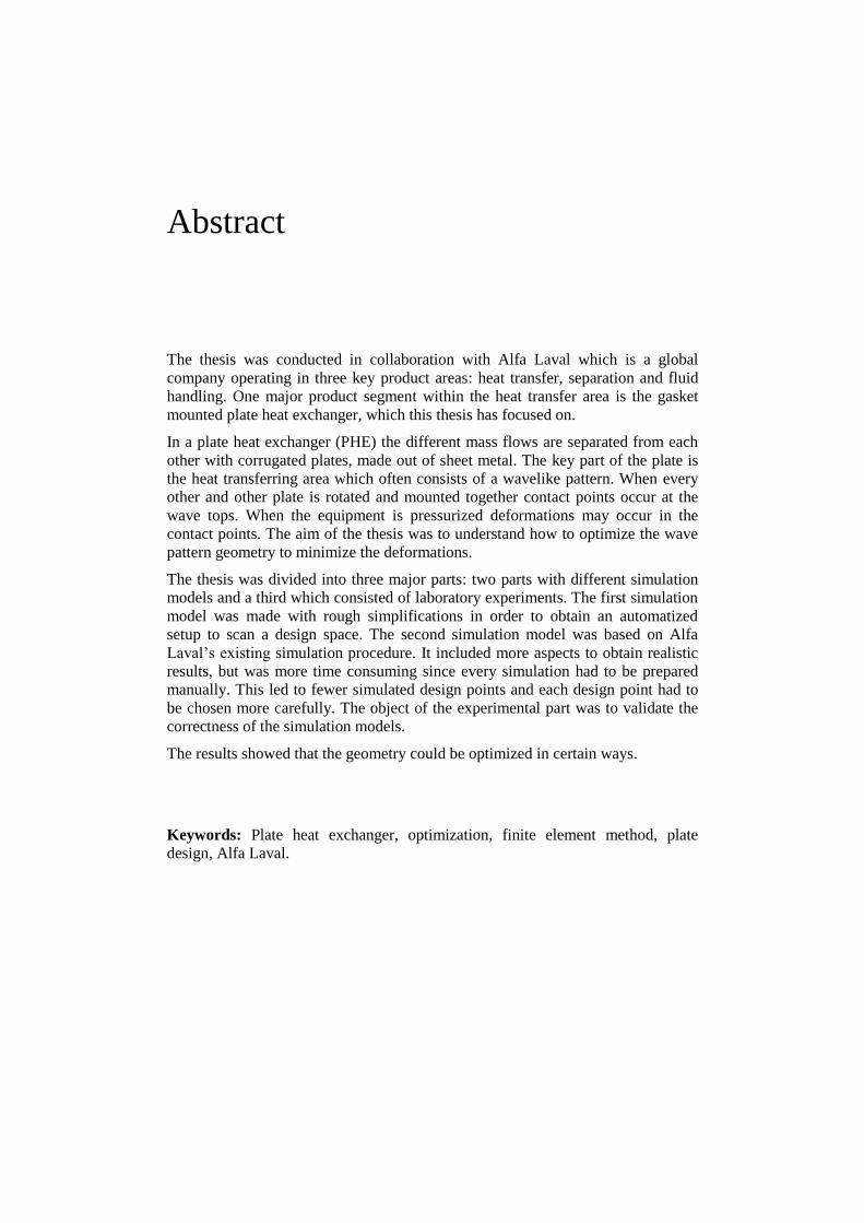
Abstract
The thesis was conducted in collaboration with Alfa Laval which is a global
company operating in three key product areas: heat transfer, separation and fluid
handling. One major product segment within the heat transfer area is the gasket
mounted plate heat exchanger, which this thesis has focused on.
In a plate heat exchanger (PHE) the different mass flows are separated from each
other with corrugated plates, made out of sheet metal. The key part of the plate is
the heat transferring area which often consists of a wavelike pattern. When every
other and other plate is rotated and mounted together contact points occur at the
wave tops. When the equipment is pressurized deformations may occur in the
contact points. The aim of the thesis was to understand how to optimize the wave
pattern geometry to minimize the deformations.
The thesis was divided into three major parts: two parts with different simulation
models and a third which consisted of laboratory experiments. The first simulation
model was made with rough simplifications in order to obtain an automatized
setup to scan a design space. The second simulation model was based on Alfa
Laval’s existing simulation procedure. It included more aspects to obtain realistic
results, but was more time consuming since every simulation had to be prepared
manually. This led to fewer simulated design points and each design point had to
be chosen more carefully. The object of the experimental part was to validate the
correctness of the simulation models.
The results showed that the geometry could be optimized in certain ways.
Keywords: Plate heat exchanger, optimization, finite element method, plate
design, Alfa Laval.

Sammanfattning
Examensarbetet gjordes i sammarbete med Alfa Laval som är ett globalt företag
verksamt inom tre huvudområden: Värmeöverföring, separering och
flödeshantering. Ett av de största produktområdena inom värmeöverföring är
packningsförsedda plattvärmeväxlare, vilket uppsatsen har fokuserat på.
I en plattvärmeväxlare hålls de olika massflödena separerade med hjälp av
korrugerade plattor gjorda av plåt. Den viktigaste delen av plattan är den
värmeöverförande ytan som består av ett vågfomat möster. När varannan platta
vrids och plattorna monteras samman uppstår kontaktpunkter på vågtopparna
mellan plattorna. När sedan utrustningen trycksätts kan det uppstå deformationer i
kontaktpunkterna. Målet med uppsatsen var att förstå hur vågmönstret kan
optimeras för att minimera dessa deformationer.
Uppsatsen delades upp i tre delar: Två olika simuleringsdelar och en tredje del
som bestod av fysiska experiment. Den första simuleringsmodellen bestod av
grova förenklingar för att kunna automatisera utforskningen av den uppställda
konstruktionsrymden. Den andra simuleringsmodellen utgick från Alfa Lavals
befintliga simuleringstillvägagångssätt. Den tar å ena sidan hänsyn till fler faktorer
och uppnår på så sätt ett mer realistiskt resultat, men tar å andra sidan mer tid då
alla förberedande steg måste göras manuellt. Detta resulterade i att färre
utformningar kunde simuleras med denna metod och att valen av
utformningspunkter blev allt viktigare. Den experimentella delen gjordes för att
validera korrektheten av simuleringmodellerna mot verkligheten.
Resultaten visade att geometrin kan optimeras.
Nyckelord: Plattvärmeväxlare, optimering, finita elementmetoden,
plattkonstruktion, Alfa Laval.


Preface
The Master Thesis has been conducted at the Department of Design Sciences,
Faculty of Engineering LTH, Lund University as a collaboration with Alfa Laval.
I would like to thank my supervisor at Alfa Laval, Joakim Krantz, for his guidance
during the work. I would also like to thank Håkan Larsson at the Mechanical
Technology department at Alfa Laval for his advice.
At the university I would like to thank my supervisor, Lecturer Per-Erik
Andersson for his support and cooperation throughout the thesis.
Lund, March 2016
Mattias Norén
Table of Contents
1 Introduction 15
1.1 The Company 15
1.2 Background 15
1.3 Ethics 17
1.4 Confidential Information 17
2 Aim 19
3 Method 21
3.1 Overview 21
3.1.1 Design Space Exploration 22
3.1.2 Forming and Pressure Simulations 22
3.1.3 Laboratory Experiments 22
3.2 Software 23
4 Limitations 25
5 Theory 27
5.1 Heat Exchangers 27
5.1.1 Function and Design of PHE 27
5.1.2 Manufacturing Process of Plates 29
5.1.3 Local and Global Deformation 29
5.2 Finite Element Method 30
5.2.1 Brief Explanation 30
5.2.2 Shell Elements and the Engineering Theory of Plates 31
5.2.3 Explicit and Implicit Solver 31
5.3 Anisotropic Material Model of Plasticity 32
6 Geometry 33
6.1 The Pressing Tool 33
6.2 Design Parameters 33
6.2.1 Constraints 34
6.2.2 Relations 35
6.3 Design Space 36
7 Design Space Exploration 37
7.1 Constraints 37
7.1.1 Geometry 37
7.1.2 Design Space 38
7.1.3 Model 40
7.2 Simulation Model Approach 41
7.2.1 Model 41
7.2.2 Material Model 42
7.2.3 Mesh 43
7.2.4 Boundary Conditions 45
7.2.5 Number of Contact Points 48
7.2.6 Friction 49
7.2.7 Other Adjustments 50
7.2.8 Zoomed in Study 50
7.2.9 Software interference 51
7.3 Post Process of Results 51
8 Forming and Pressure Simulations 53
8.1 Purpose 53
8.2 Constraints 53
8.2.1 Theoretical Plate Angle 53
8.2.2 Settings 54
8.2.3 Material Model 54
8.2.4 Global Deformation 54
8.2.5 Design Points 55
8.3 Simulation Model Approach 55
8.3.1 Model 55
8.3.2 Material Model 55
8.3.3 Boundary Conditions 56
8.3.4 Mesh 56
8.3.5 Forming Simulation 57
8.3.6 Pressure Simulation 57
8.4 Post Process of Results 59
8.4.1 Measurement 59
9 Laboratory Experiments 61
9.1 Constraints 61
9.2 Experimental Approach 61
9.2.1 Pressure Levels 61
9.2.2 Material 62
9.2.3 Measurement 63
9.2.4 Post Processing of Results 64
10 Results 67
10.1 Design Space Exploration 67
10.1.1 Initial Design Space Exploration 67
10.1.2 Zoomed in Study 69
10.2 Forming and Pressure Simulations 70
10.3 Comparison of Design Optimization Results 75
10.4 Laboratory Experiments 77
10.5 Verification of Simulation Models 78
11 Discussion 79
11.1 Design Exploration Simulations 79
11.2 Forming and Pressure Simulations 80
11.3 Laboratory Experiments 81
11.4 Comparison of Results 82
11.4.1 Verification of Simulation Models with Experiments 82
11.4.2 Design Optimization 82
11.5 General Improvements 83

11.6 Thoughts 83
11.7 Conclusions 87
11.8 Recommendations for Future Work 87
References 89
Appendix A Time Schedule
Appendix B Theoretical and True Plate Angle

15
1 Introduction
This chapter gives an introduction to the thesis. It includes a description of the
company, the background of the project with a short brief of a plate heat
exchanger and what problems that initiated the thesis.
1.1 The Company
Alfa Laval is a global company with three key product areas: heat transfer,
separation and fluid handling. It all started in 1883 when Gustav de Laval and
Oscar Lamm Jr founded the company Separator AB, which in 1963 became Alfa
Laval. Today Alfa Laval holds more than 2000 patents, their products are sold in
approximately 100 countries with 18,000 employees worldwide. In 2014 Alfa
Laval had sales of 35.1 billion SEK. The head office is located in Lund, Sweden,
which is also where the major part of the research and development of plate heat
exchangers (PHE) is done [1].
1.2 Background
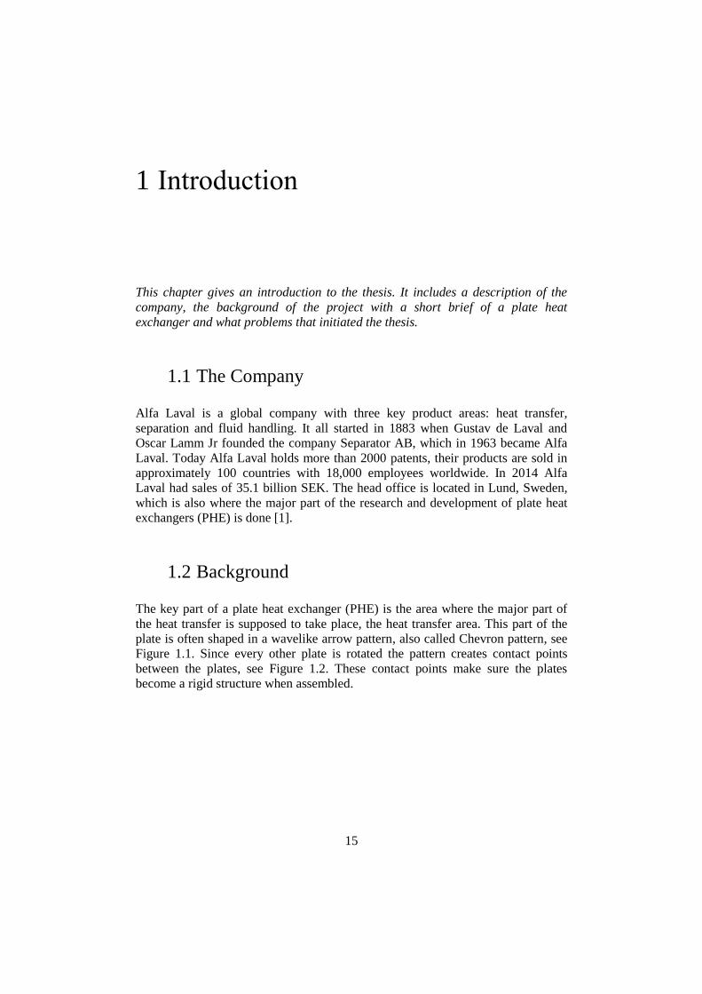
The key part of a plate heat exchanger (PHE) is the area where the major part of
the heat transfer is supposed to take place, the heat transfer area. This part of the
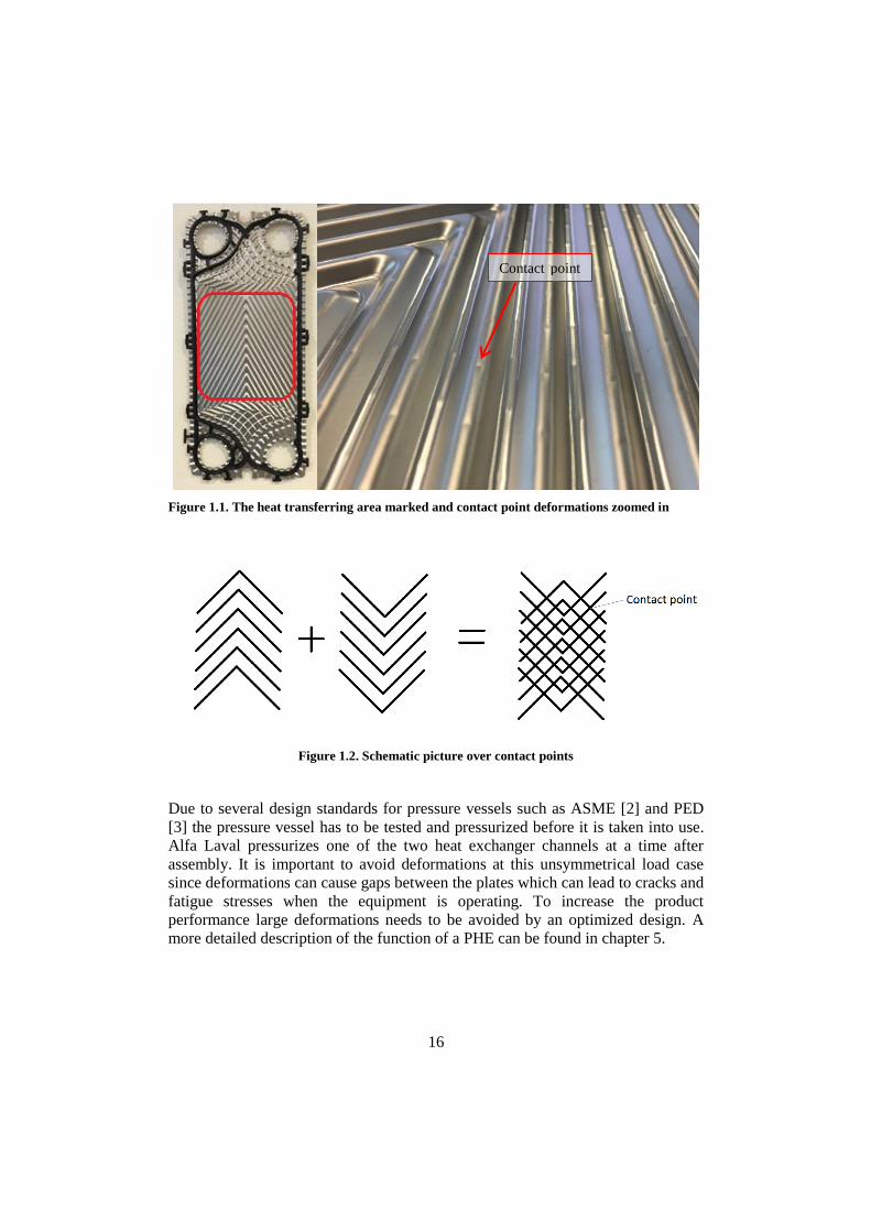
plate is often shaped in a wavelike arrow pattern, also called Chevron pattern, see
Figure 1.1. Since every other plate is rotated the pattern creates contact points
between the plates, see Figure 1.2. These contact points make sure the plates
become a rigid structure when assembled.
16
Figure 1.1. The heat transferring area marked and contact point deformations zoomed in
Figure 1.2. Schematic picture over contact points
Due to several design standards for pressure vessels such as ASME [2] and PED
[3] the pressure vessel has to be tested and pressurized before it is taken into use.
Alfa Laval pressurizes one of the two heat exchanger channels at a time after
assembly. It is important to avoid deformations at this unsymmetrical load case
since deformations can cause gaps between the plates which can lead to cracks and
fatigue stresses when the equipment is operating. To increase the product
performance large deformations needs to be avoided by an optimized design. A
more detailed description of the function of a PHE can be found in chapter 5.
Contact point
def.

17
1.3 Ethics
There are no obvious ethical problems with heat exchangers compared with e.g.
the weapon industry. In many applications heat exchangers are used to minimize
the waste of energy in processes by preheating an incoming mass flow with an
outgoing. Since energy production more or less always has a negative impact on
the environment through emissions or exploitation of nature a minimization of the
consumed energy for a certain process is positive. Since heat exchangers are
general products with a broad spectrum of application areas it is up to the user to
decide whether it is to be used for a good or bad cause. Despite this there are
obvious situations where the reseller has a responsibility to make sure the
equipment is not sold to e.g. terrorist organizations.
A heat exchanger can reduce the cost of a process, e.g. in the oil industry. In this
sector the heat exchanger can be a contributing part in making it profitable to
extract fossil oil which has a negative impact on the environment if it is
combusted. However, a heat exchanger can contribute to making production of
renewable energy more efficient and profitable which in the long term can reduce
negative impact on the environment. In both cases the heat exchanger can reduce
the waste of energy, which is positive. This argumentation strengthens that there
are no ethical problems with working with development of heat exchangers.
1.4 Confidential Information
Some information regarding the Alfa Laval products such as material models,
geometry and results were seen as confidential. This means that some parameter
values could not be revealed and had to be presented in general terms. Some
figures are not as detailed as they could have been and some scales have been
removed or modified. In some places where it might look strange that no values
are revealed there are footnotes marking the confidential information.

19
2 Aim
The general aim of the thesis is presented below.
The thesis was initiated to increase the knowledge of how different parameters
affect the strength and deformation of the heat exchanger plates in contact points
of the heat transfer area. The aim was to understand how to optimize the design to
minimize the deformations. If no specific optimal design was obtained the
objective was to find design guidelines on how to minimize the deformations.
It was of interest to investigate how different simulation models work and match
the experimental results. The forming and pressure simulation routine was known
to be functional but a more detailed verification against reality was of interest. The
design space exploration simulations were known to be roughly simplified. It was
still of interest to see how those kinds of simplifications would affect the results
and if the method could be used in order to optimize the results by comparing
them relatively to each other.

21
3 Method
This chapter describes the general and overall method of the thesis. More detailed
simulation and experiment method descriptions are given in each subsection.
3.1 Overview
No conventional scientific overall method was used in the thesis. The method can
rather be seen as a description of a product development procedure to obtain more
information about the behavior of a product. Despite this, the well accepted Finite
Element Method (FEM) was used as the main tool in solving the task. Other
conventional engineering tools such as computational CAD-modulation and
analytical mathematics were also used.
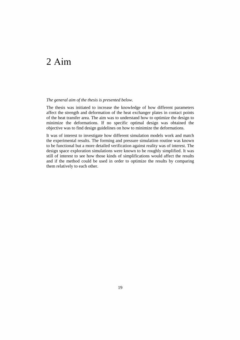
The thesis consists of three major parts. The two first parts handle different ways
to model and simulate in a theoretical manner. The purpose of these simulations
was to find an optimal design or at least a suitable design space. The third part was
made to verify the theoretical models with laboratory experiments. A schematic
picture of the thesis is seen in Figure 3.1.
Figure 3.1. Schematic overview of the thesis
Design space exploration
Forming and pressure
simulations
Laboratory experiments
Comparison and verification of results
Results of optimization
22
Each of the three major parts is described in more detail in separate chapters. Here
follows a brief introduction to the three parts to make it possible to get an
overview.
3.1.1 Design Space Exploration
This part of the thesis was made to explore the design space with a larger amount
of design points than what was made in the forming and pressure simulation part.
To be able to run all of the simulations within a reasonable time a lot of
simplifications had to be made. The most important aspect was that the forming
process was neglected and the geometry was controlled directly in the CAD
software, Creo. A test matrix was set up and all the simulations could be run
automatically from that. Ansys workbench was used to solve this FEM task. An
existing Alfa Laval plate, further on denoted as “the reference plate”, was
simulated in two plate thicknesses to verify the model by laboratory experiments.
3.1.2 Forming and Pressure Simulations
With the results from the design space exploration some verifying simulations in
the interesting design space area were performed. In this part, the forming process
was included and also a more detailed material model was adopted. Each design
point had to be manually prepared which made it more time consuming than the
simulations in the design space exploration. The software used for this task was
Creo and Dynaform for preparation of the model. Ls-dyna, which used an explicit
solver instead of an implicit as Ansys did, was used to solve this FEM task. The
difference between explicit and implicit solving method is described in the theory
chapter. This simulation model was also used to simulate the reference plate in
order to verify the model by laboratory experiments.
3.1.3 Laboratory Experiments
To verify the simulated results some experimental tests had to be done. Two
different plate thicknesses of the reference plate were pressurized to four different
pressure levels each, i.e. eight tests. The tests were made at Alfa Laval’s
laboratory in Lund. Afterwards, the results were compared to the simulations to
see if the theoretical models were reliable.

23
3.2 Software
The software listed below was used in the thesis and all licenses were supplied by
Alfa Laval.
Creo 2.0
Ansys workbench 16.0
Dynaform 5.9.1
LS-dyna
Microsoft Word, Excel and Project 2010

25
4 Limitations
The limitations of the thesis are defined in this chapter.
Overall limitations for the thesis were made to achieve a well-defined project
manageable within the time schedule. A Master Thesis time limit is one semester
or approximately 20 weeks and as a consequence, the extent of the thesis must be
restricted. The overall limitations are listed below:
Only the mechanical aspects of the design were examined. This means no
consideration of the heat transfer or flow aspects were evaluated even
though they are affected by the design.
Exclusively Chevron patterned heat transfer areas were investigated.
Only contact points of the heat transferring area were investigated.
The plate material was limited to stainless steel, Alloy 316.
The interaction of two identical plates was investigated and accordingly
plates with different Chevron angles were not mixed. However, the results
may be applicable on a mixed setup.
Shell elements were adopted in the simulation models.
The geometry optimization simulations were performed with 0.5 mm in
plate thickness.
The verification of the simulation models made by laboratory experiments
were implemented with both 0.5 mm and 0.4 mm plate thicknesses.
The reference plate was used as a base in the modulation geometries.
Only the reference plate’s pressing depth, which is about 4 mm, was used.
The reference plate was used to verify the theoretical model with reality
through the laboratory experiments.

27
5 Theory
This chapter gives explanations of the mechanisms and theories which are
fundamental to the thesis.
5.1 Heat Exchangers
There are several different types of heat exchangers such as tube or spiral heat
exchangers but this thesis focus on plate heat exchangers (PHE). There are in
general two types of PHEs, gasket mounted (GPHE) and brazed (BHE). In BHE
all plates are brazed together and they cannot be disassembled to be cleaned or
serviced. They are often used in smaller applications such as heat pumps or district
heating systems in both private houses and apartment houses. GPHE are in general
larger than BHE and are used when larger capacity is needed or possibilities of
cleaning and servicing are important. Examples of applications for GPHE are:
Chemical process industries, dairies, breweries, ships, greater buildings etc. This
means that the media which is handled could be anything from corrosive acids, oil
and seawater to milk and cream.
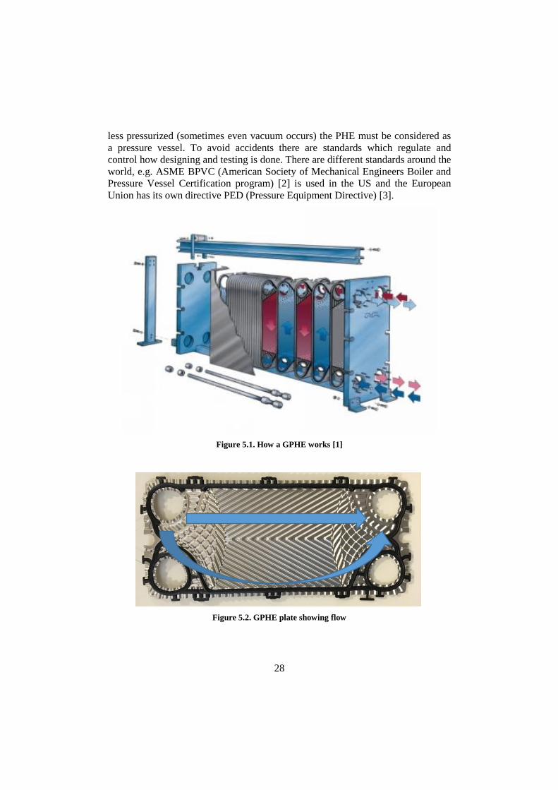
5.1.1 Function and Design of PHE
The purpose with a heat exchanger is to transfer heat energy from one media to
another without mixing them together. PHE are made from corrugated plates
which separate the flows from each other at the same time as they transfer the
heat. The pattern of the corrugated plates are made to maximize the area, increase
the flow turbulence, distribute the flows over the plates and separate the plates
from each other to create flow channels. GPHE have gaskets as seal and the
gaskets also make sure the flows are separated. The gaskets are most commonly
attached at the edge of the plates but some gaskets need to be glued to stay
attached when the equipment is assembled or opened. It is most common that the
plates are in principal identical throughout the apparatus. Every other plate is
rotated 180 degrees which makes half of the channels filled with warm and half
with cold media, see Figure 5.1 and Figure 5.2. Outside of the heat transferring
plates there are two thicker plates, frame and pressure plates, which hold the plate
package together with bolts. Since the flows through the PHE are always more or
28
less pressurized (sometimes even vacuum occurs) the PHE must be considered as
a pressure vessel. To avoid accidents there are standards which regulate and
control how designing and testing is done. There are different standards around the
world, e.g. ASME BPVC (American Society of Mechanical Engineers Boiler and
Pressure Vessel Certification program) [2] is used in the US and the European
Union has its own directive PED (Pressure Equipment Directive) [3].
Figure 5.1. How a GPHE works [1]
Figure 5.2. GPHE plate showing flow
29
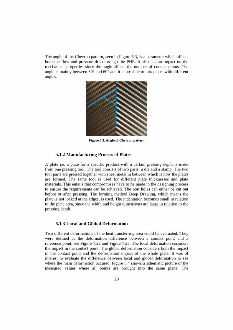
The angle of the Chevron pattern, seen in Figure 5.3, is a parameter which affects
both the flow and pressure drop through the PHE. It also has an impact on the
mechanical properties since the angle affects the number of contact points. The
angle is mainly between 30° and 60° and it is possible to mix plates with different
angles.
Figure 5.3. Angle of Chevron pattern
5.1.2 Manufacturing Process of Plates
A plate i.e. a plate for a specific product with a certain pressing depth is made
from one pressing tool. The tool consists of two parts: a die and a stamp. The two
tool parts are pressed together with sheet metal in between which is how the plates
are formed. The same tool is used for different plate thicknesses and plate
materials. This entails that compromises have to be made in the designing process
to ensure the requirements can be achieved. The port holes can either be cut out
before or after pressing. The forming method Deep Drawing, which means the
plate is not locked at the edges, is used. The indentation becomes small in relation
to the plate area, since the width and height dimensions are large in relation to the
pressing depth.
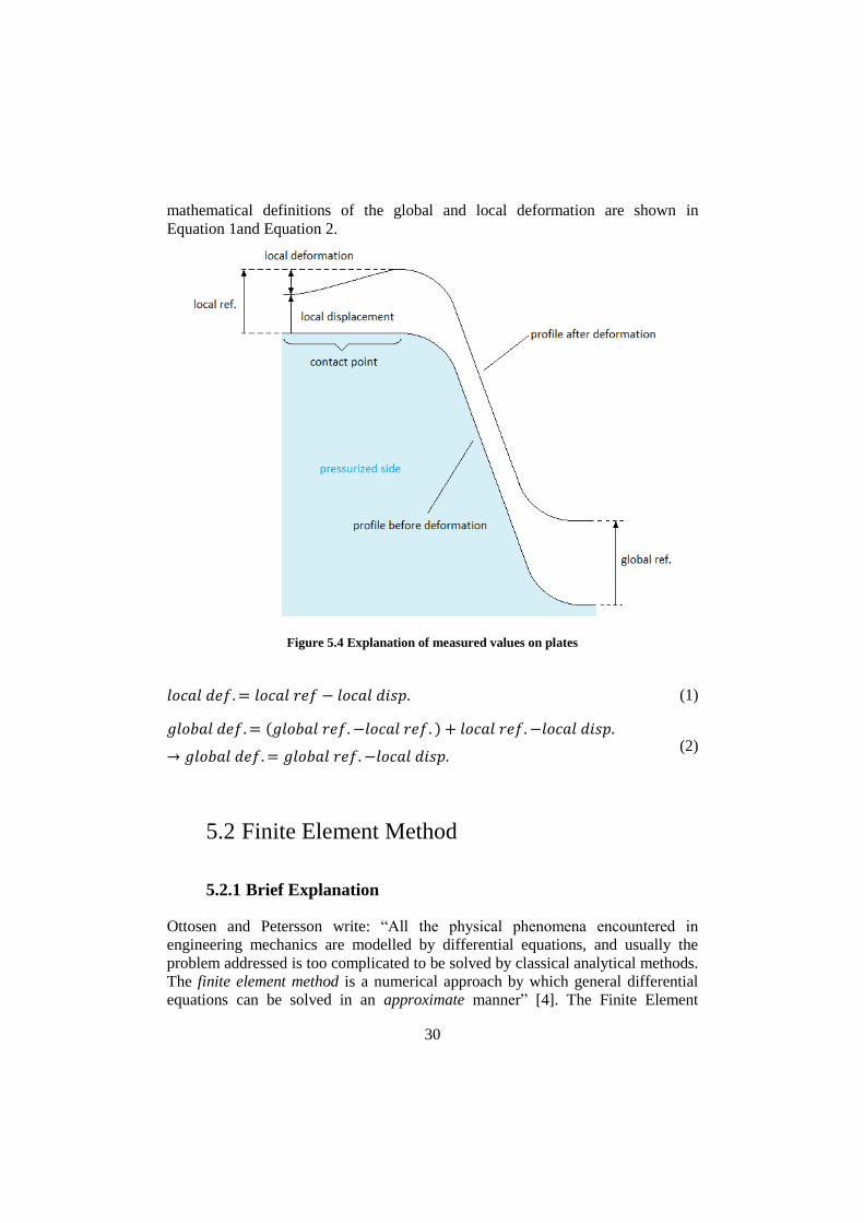
5.1.3 Local and Global Deformation
Two different deformations of the heat transferring area could be evaluated. They
were defined as the deformation difference between a contact point and a
reference point, see Figure 7.22 and Figure 7.23. The local deformation considers
the impact in the contact point. The global deformation considers both the impact
in the contact point and the deformation impact of the whole plate. It was of
interest to evaluate the difference between local and global deformation to see
where the main deformation occured. Figure 5.4 shows a schematic picture of the
measured values where all points are brought into the same plane. The
30
mathematical definitions of the global and local deformation are shown in
Equation 1and Equation 2.
Figure 5.4 Explanation of measured values on plates
𝑙𝑜𝑐𝑎𝑙 𝑑𝑒𝑓. = 𝑙𝑜𝑐𝑎𝑙 𝑟𝑒𝑓 − 𝑙𝑜𝑐𝑎𝑙 𝑑𝑖𝑠𝑝. (1)
𝑔𝑙𝑜𝑏𝑎𝑙 𝑑𝑒𝑓. = (𝑔𝑙𝑜𝑏𝑎𝑙 𝑟𝑒𝑓. −𝑙𝑜𝑐𝑎𝑙 𝑟𝑒𝑓. ) + 𝑙𝑜𝑐𝑎𝑙 𝑟𝑒𝑓. −𝑙𝑜𝑐𝑎𝑙 𝑑𝑖𝑠𝑝.
→ 𝑔𝑙𝑜𝑏𝑎𝑙 𝑑𝑒𝑓. = 𝑔𝑙𝑜𝑏𝑎𝑙 𝑟𝑒𝑓. −𝑙𝑜𝑐𝑎𝑙 𝑑𝑖𝑠𝑝. (2)
5.2 Finite Element Method
5.2.1 Brief Explanation
Ottosen and Petersson write: “All the physical phenomena encountered in
engineering mechanics are modelled by differential equations, and usually the
problem addressed is too complicated to be solved by classical analytical methods.
The finite element method is a numerical approach by which general differential
equations can be solved in an approximate manner” [4]. The Finite Element
31
Method (FEM) is widely used for research and development applications. It is
applicable in many fields and especially suitable to solve static and dynamic
mechanical problems. To solve mechanical problems the geometry is needed.
Most commonly the geometry is modulated with CAD software and imported to
the numerical solving software. From the 3D model a mesh is generated to define
the geometry in mathematical terms. A mesh is a grid system defined by elements
and nodes. In mechanical applications one, two and three dimensional elements
can be used. A material model can be needed to define the behavior of the
elements if e.g. the deformation is of interest. Constraints which define the
boundary conditions in some certain nodes are needed to obtain a solvable model.
5.2.2 Shell Elements and the Engineering Theory of Plates
For both of the simulation models used in the thesis shell elements were chosen
instead of solid elements. Ottosen and Peterson write about shell elements in FEM:
“…the theory of plates is an engineering approximation which reduces the original
three-dimensional problem to a simpler two-dimensional problem. For many
applications, however, this engineering theory provides realistic solutions,
especially if the plate is thin.” [4]. This means there will be no variation of the
result over the thickness. They also write: “Generally speaking, a plate is a
structure with a thickness t that is small compared with all other dimensions of the
plate…” and “…a plate is loaded by forces normal to the plane of the plate.” [4].
The ratio between plate thickness and other dimensions needed to assume The
Theory of Plate is not specifically determined. The greater difference between
thickness and other dimensions the better approximation will be obtained. Plates
of PHE often have a thickness, t, smaller than a millimeter and the overall
dimensions are in the scale of meters.
5.2.3 Explicit and Implicit Solver
Two different solving methods for the FEM differential equation were used for the
simulation models, explicit and implicit method. The design space exploration
simulation model which was solved with Ansys used the implicit method. The
more complex model, which included the plate forming, used the explicit method
by the software of Ls-dyna. Some practical information about the differences
between explicit and implicit solver were found on the Ls-dyna support webpages:
“In nonlinear implicit analysis, solution of each step requires a series of trial
solutions (iterations) to establish equilibrium within a certain tolerance. In explicit
analysis, no iteration is required as the nodal accelerations are solved directly.”
[5].
32
“The time step in explicit analysis must be less than the Courrant time step (time it
takes a sound wave to travel across an element). Implicit transient analysis has no
inherent limit on the size of the time step. As such, implicit time steps are
generally several orders of magnitude larger than explicit time steps.” [5].
“Explicit analysis handles nonlinearities with relative ease as compared to implicit
analysis. This would include treatment of contact and material nonlinearities.” [5].
“Implicit analysis requires a numerical solver to invert the stiffness matrix once or
even several times over the course of a load/time step. This matrix inversion is an
expensive operation, especially for large models. Explicit doesn't require this
step.” [5].
5.3 Anisotropic Material Model of Plasticity
The sheet metal gets anisotropic material properties caused by the forming
process. Therefore an anisotropic material model was adopted in the forming and
pressure simulations. The model was based on a planar-stress yield criterion for
orthotropic anisotropy which Barlat and Lian presented in 1989, shown by
Equation 3, 4 and 5. [6].
𝑓 = 𝑎|𝐾1 + 𝐾2|𝑀 + 𝑎|𝐾1 − 𝐾2|𝑀 + 𝑐|2𝐾2|𝑀 = 2�̅�𝑀 (3)
Where:
𝐾1 =𝜎𝑥𝑥 + ℎ𝜎𝑦𝑦
2 (4)
𝐾2 = √(𝜎𝑥𝑥 − ℎ𝜎𝑦𝑦
2)
2
+ 𝑝2𝜎𝑥𝑦2 (5)
�̅� is the uniaxial yield stress in the rolling direction
𝑀 is a material coefficient e.g.:
𝑀 = 6 for a BCC material (Body Center Cubic structure)
𝑀 = 8 for a FCC material (Face Center Cubic structure).
𝑎, 𝑐, 𝑝 and ℎ are material constants which can be calculated from 𝑅 values
obtained from uniaxial tension tests in three directions, for instance 𝑅0, 𝑅45 and
𝑅90. The 𝑅 values are ratios between strains in two directions. For more details see
the article by Barlat F. and Lian J. [6]
33
6 Geometry
This section examines the geometry and conditions that have to be taken into
account when modulating and simulating. All equations are derived from the
geometry.
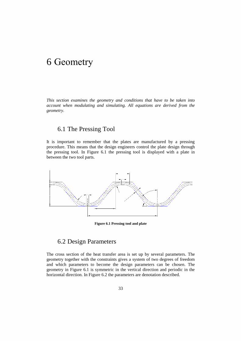
6.1 The Pressing Tool
It is important to remember that the plates are manufactured by a pressing
procedure. This means that the design engineers control the plate design through
the pressing tool. In Figure 6.1 the pressing tool is displayed with a plate in
between the two tool parts.
Figure 6.1 Pressing tool and plate
6.2 Design Parameters
The cross section of the heat transfer area is set up by several parameters. The
geometry together with the constraints gives a system of two degrees of freedom
and which parameters to become the design parameters can be chosen. The
geometry in Figure 6.1 is symmetric in the vertical direction and periodic in the
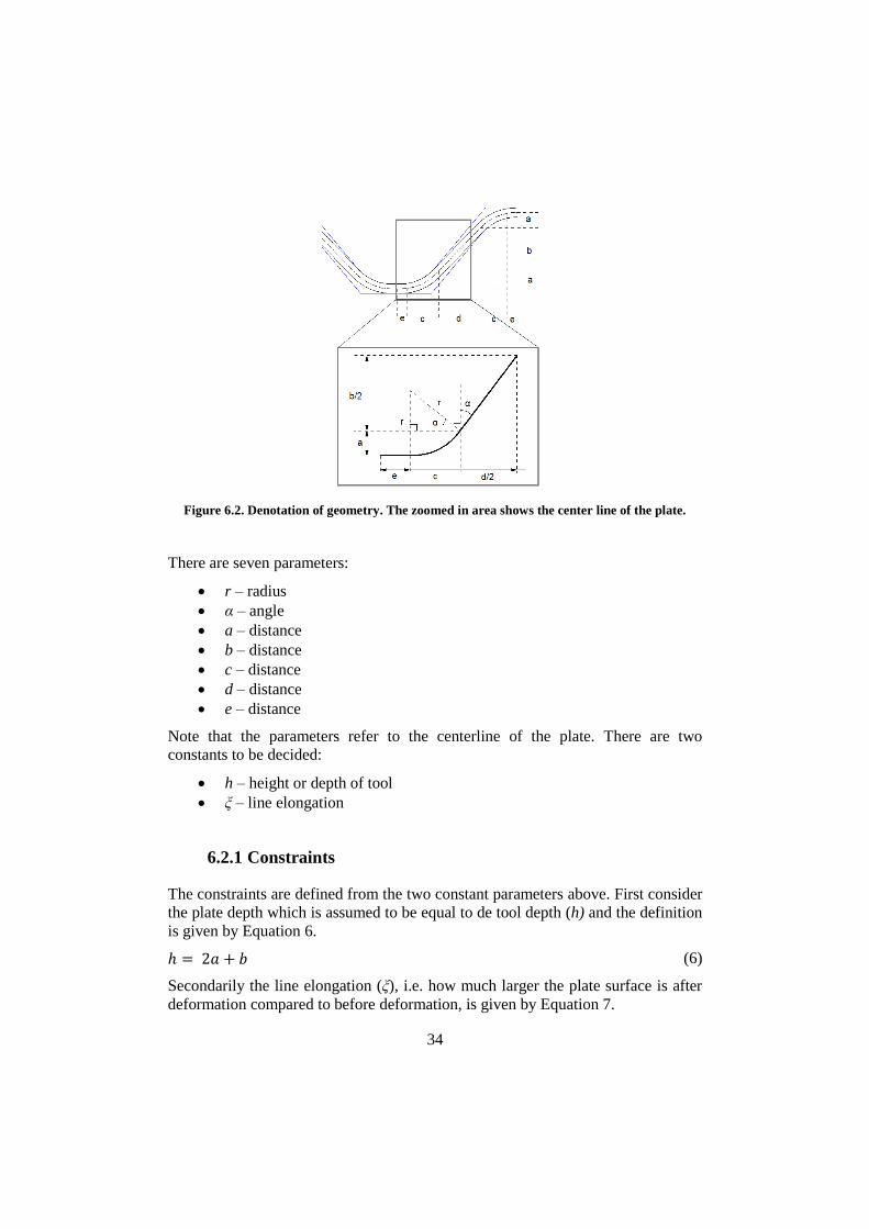
horizontal direction. In Figure 6.2 the parameters are denotation described.
34
Figure 6.2. Denotation of geometry. The zoomed in area shows the center line of the plate.
There are seven parameters:
r – radius
α – angle
a – distance
b – distance
c – distance
d – distance
e – distance
Note that the parameters refer to the centerline of the plate. There are two
constants to be decided:
h – height or depth of tool
ξ – line elongation
6.2.1 Constraints
The constraints are defined from the two constant parameters above. First consider
the plate depth which is assumed to be equal to de tool depth (h) and the definition
is given by Equation 6.
ℎ = 2𝑎 + 𝑏 (6)
Secondarily the line elongation (ξ), i.e. how much larger the plate surface is after
deformation compared to before deformation, is given by Equation 7.

35
𝜉 =𝑒 + 𝑟𝜋
90 − 𝛼180
+𝑏
2 cos 𝛼
𝑒 + 𝑐 +𝑑2
(7)
6.2.2 Relations
From Figure 6.2 Equations 8 and 9 can be derived.
𝑎 = 𝑟(1 − sin 𝛼) (8)
𝑐 = 𝑟 cos 𝛼 (9)
Equations 6 and 8 combined gives Equation 10.
𝑏 = ℎ − 2𝑎 = ℎ − 2𝑟(1 − sin 𝛼) (10)
The geometry in Figure 6.2 also gives Equation 11.
𝑑 = 𝑏 tan 𝛼 = (ℎ − 2𝑟(1 − sin 𝛼)) tan 𝛼 (11)
Equation 7 with inserted expressions from Equations 9, 10 and 11 gives Equation
12.
𝜉 =𝑒 + 𝑟𝜋
90 − 𝛼180
+𝑏
2 cos 𝛼
𝑒 + 𝑐 +𝑑2
=𝑒 + 𝑟𝜋
90 − 𝛼180
+
ℎ2
− 𝑟(1 − sin 𝛼)
cos 𝛼
𝑒 + 𝑟 cos 𝛼 + (ℎ2 − 𝑟(1 − sin 𝛼)) tan 𝛼
(12)
Equation 12 can be described either as a function 𝑟(𝑒, 𝛼) (Equation 13) or as a
function 𝑒(𝑟, 𝛼) (Equation 14).
𝑟 =
ℎ2
cos 𝛼 − (𝜉 − 1)𝑒 − 𝜉ℎ2 tan 𝛼
𝜉(cos 𝛼 − (1 − sin 𝛼) tan 𝛼) − 𝜋90 − 𝛼
180 +1 − sin 𝛼
cos 𝛼
(13)
𝑒 =
𝑟𝜋90 − 𝛼
180+
ℎ2 − 𝑟(1 − sin 𝛼)
cos 𝛼− 𝜉(𝑟 cos 𝛼 + (
ℎ2 − 𝑟(1 − sin 𝛼)) tan 𝛼)
(𝜉 − 1) (14)
Now an equation system with two degrees of freedom is obtained from the seven
parameters and the five equations, 8 to 12. When choosing which parameters to be
free, i.e. the design parameters, there are some alternatives. The flat surface 𝑒, the
radius 𝑟, and the angle 𝛼 are all possible, but only two can be chosen. It was seen
that it was easiest to graphically interpret the design space as a function of radius
and angle and therefore they were chosen as design parameters.
36
All equations were verified by CAD-models and drawings, i.e. known design
parameters from an existing plate where the input and the output were compared to
the existing plate.
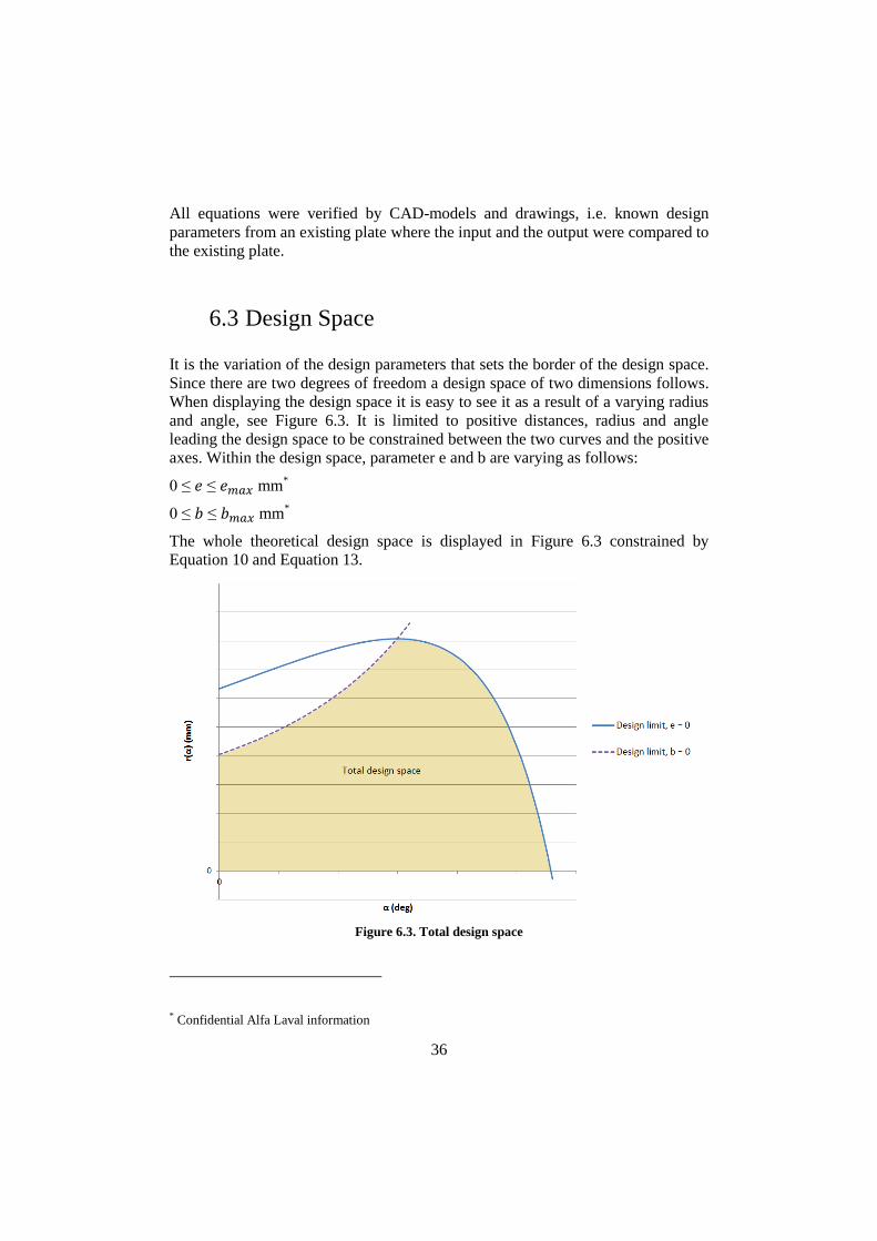
6.3 Design Space
It is the variation of the design parameters that sets the border of the design space.
Since there are two degrees of freedom a design space of two dimensions follows.
When displaying the design space it is easy to see it as a result of a varying radius
and angle, see Figure 6.3. It is limited to positive distances, radius and angle
leading the design space to be constrained between the two curves and the positive
axes. Within the design space, parameter e and b are varying as follows:
0 ≤ 𝑒 ≤ 𝑒𝑚𝑎𝑥 mm*
0 ≤ 𝑏 ≤ 𝑏𝑚𝑎𝑥 mm*
The whole theoretical design space is displayed in Figure 6.3 constrained by
Equation 10 and Equation 13.
Figure 6.3. Total design space
* Confidential Alfa Laval information
37
7 Design Space Exploration
The design space exploration part of the thesis aimed to get a brief picture of the
deformation behavior over the interesting part of the design space. The interesting
part of the design space refers to the part which is reasonable to manufacture and
design. The aim was to get results for several design points to be able to plot the
results over the design space. This would make it possible to see which area could
be interesting for further investigations. It also aimed verify the simulation model
with the laboratory experiments
7.1 Constraints
7.1.1 Geometry
The plate depth that was chosen to use was equal to the reference plate depth*.
Inserted in Equation 6 it gave Equation 15.
2𝑎 + 𝑏 = ℎ𝑟𝑒𝑓. mm (15)
The line elongation was set to a value which was common for Alfa Laval’s plates,
𝜉𝑐𝑜𝑚.*. Inserted in Equation 7 it gave Equation 16.
𝑒 + 𝑟𝜋90 − 𝛼
180 +𝑏
2 cos 𝛼
𝑒 + 𝑐 +𝑑2
= 𝜉𝑐𝑜𝑚. (16)
The line elongation value was selected before the reference plate line elongation
value was known. Therefore, the verifying simulations were run with a different
line elongation than and the design space exploration and forming and pressure
simulations. The values differed one percent unit and did not affect the results
since no comparison were made between them.
* Confidential Alfa Laval information
38
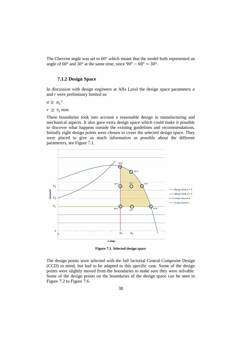
The Chevron angle was set to 60° which meant that the model both represented an
angle of 60° and 30° at the same time, since 90° − 60° = 30°.
7.1.2 Design Space
In discussion with design engineers at Alfa Laval the design space parameters α
and r were preliminary limited as:
𝛼 ≥ 𝛼1°
𝑟 ≥ 𝑟1 𝑚𝑚
These boundaries took into account a reasonable design in manufacturing and
mechanical aspects. It also gave extra design space which could make it possible
to discover what happens outside the existing guidelines and recommendations.
Initially eight design points were chosen to cover the selected design space. They
were placed to give as much information as possible about the different
parameters, see Figure 7.1.
Figure 7.1. Selected design space
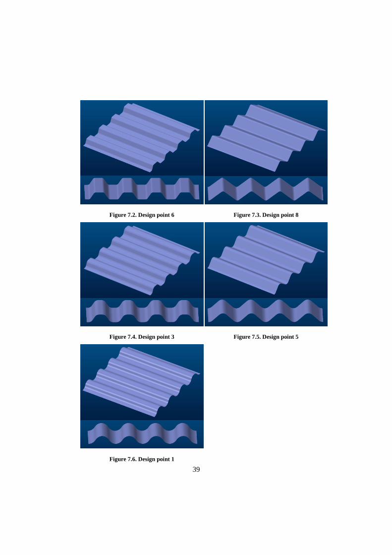
The design points were selected with the full factorial Central Composite Design
(CCD) in mind, but had to be adapted to this specific case. Some of the design
points were slightly moved from the boundaries to make sure they were solvable.
Some of the design points on the boundaries of the design space can be seen in
Figure 7.2 to Figure 7.6.
𝛼1 𝛼2
𝑟3
𝑟2
𝑟1
39
Figure 7.2. Design point 6 Figure 7.3. Design point 8
Figure 7.4. Design point 3 Figure 7.5. Design point 5
Figure 7.6. Design point 1
40
After the results of the first design exploration were obtained further studies were
made. To see where a possible optimum could be the design points for the
zoomed-in study were selected more arbitrarily step by step as the results were
obtained. This is why the design points were not evenly distributed.
7.1.3 Model
The hydrostatic pressure difference between the upper and lower part of the
channels caused by the gravitation was neglected i.e. a homogeneous pressure was
applied.
Effects from the forming process were neglected since the model was modulated
directly in CAD. This means that there were no internal stresses or local thinning
of the plate caused by the forming process, which probably has a significant
impact on the results. This simplification is further discussed in chapter 11.
The plates in a GPHE are pressed together by a frame with bolts. When mounted
together an initial pressure on the plates and gaskets is created. After a while the
pressure decreases due to relaxation of the gaskets but there will always be a
remaining built in pressure. This pressure was neglected in these simulations.
41
7.2 Simulation Model Approach
Due to the fact that the study is a design space exploration a large amount of
simulations were planned. To do this within an acceptable calculation time with
the available computer capacity some simplifications had to be made. To decide
how the model could be set up, several investigations and test simulations had to
be made; thus a way of how evaluating the results also had to be defined.
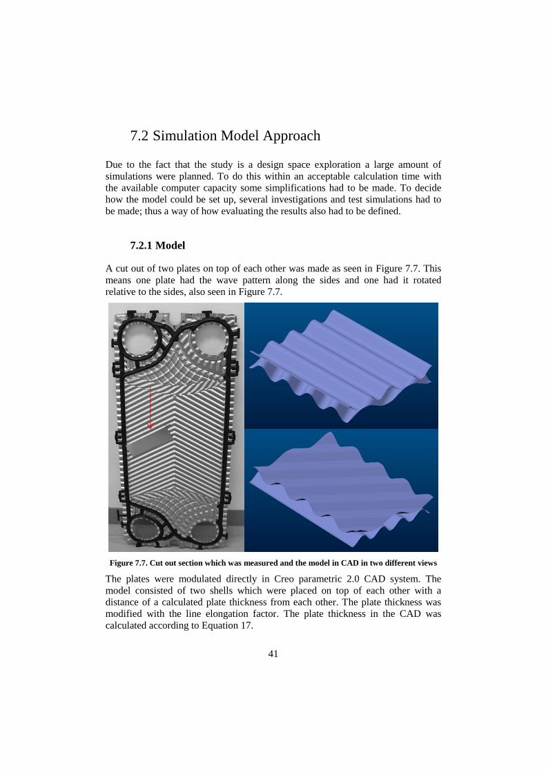
7.2.1 Model
A cut out of two plates on top of each other was made as seen in Figure 7.7. This
means one plate had the wave pattern along the sides and one had it rotated
relative to the sides, also seen in Figure 7.7.
Figure 7.7. Cut out section which was measured and the model in CAD in two different views
The plates were modulated directly in Creo parametric 2.0 CAD system. The
model consisted of two shells which were placed on top of each other with a
distance of a calculated plate thickness from each other. The plate thickness was
modified with the line elongation factor. The plate thickness in the CAD was
calculated according to Equation 17.
42
𝐩𝐥𝐚𝐭𝐞 𝐭𝐡𝐢𝐜𝐤𝐧𝐞𝐬𝐬 =𝟎. 𝟓 𝐦𝐦
𝝃𝒄𝒐𝒎.
(17)
The thickness for the verifying simulations was calculated in the same way.
As already mentioned, it was decided that the model would consist of shell
elements instead of solid element since the thickness was considered negligible in
relation to the area of the plate. With shell elements there is no variation of the
results in the thickness direction and this was considered to be an acceptable
simplification.
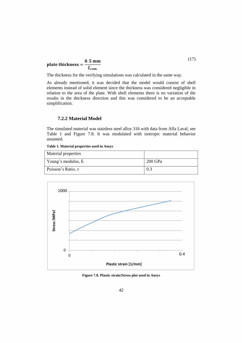
7.2.2 Material Model
The simulated material was stainless steel alloy 316 with data from Alfa Laval, see
Table 1 and Figure 7.8. It was modulated with isotropic material behavior
assumed.
Table 1. Material properties used in Ansys
Material properties
Young’s modulus, E 200 GPa
Poisson’s Ratio, v 0.3
Figure 7.8. Plastic strain/Stress plot used in Ansys
0
200
400
600
800
1000
1200
0 0,1 0,2 0,3 0,4 0,5
Stre
ss [
MP
a]
Plastic strain [1/mm]
1000
1000
0.4
43
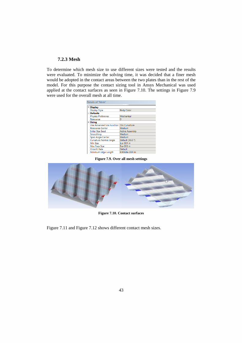
7.2.3 Mesh
To determine which mesh size to use different sizes were tested and the results
were evaluated. To minimize the solving time, it was decided that a finer mesh
would be adopted in the contact areas between the two plates than in the rest of the
model. For this purpose the contact sizing tool in Ansys Mechanical was used
applied at the contact surfaces as seen in Figure 7.10. The settings in Figure 7.9
were used for the overall mesh at all time.
Figure 7.9. Over all mesh settings
Figure 7.10. Contact surfaces
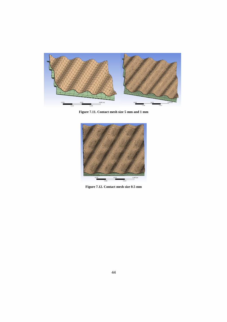
Figure 7.11 and Figure 7.12 shows different contact mesh sizes.
44
Figure 7.11. Contact mesh size 5 mm and 1 mm
Figure 7.12. Contact mesh size 0.5 mm
45
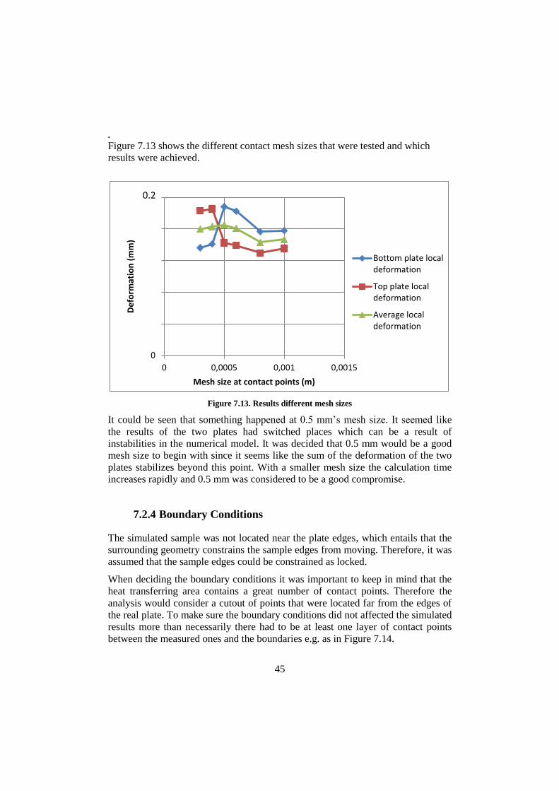
. Figure 7.13 shows the different contact mesh sizes that were tested and which
results were achieved.
Figure 7.13. Results different mesh sizes
It could be seen that something happened at 0.5 mm’s mesh size. It seemed like
the results of the two plates had switched places which can be a result of
instabilities in the numerical model. It was decided that 0.5 mm would be a good
mesh size to begin with since it seems like the sum of the deformation of the two
plates stabilizes beyond this point. With a smaller mesh size the calculation time
increases rapidly and 0.5 mm was considered to be a good compromise.
7.2.4 Boundary Conditions
The simulated sample was not located near the plate edges, which entails that the
surrounding geometry constrains the sample edges from moving. Therefore, it was
assumed that the sample edges could be constrained as locked.
When deciding the boundary conditions it was important to keep in mind that the
heat transferring area contains a great number of contact points. Therefore the
analysis would consider a cutout of points that were located far from the edges of
the real plate. To make sure the boundary conditions did not affected the simulated
results more than necessarily there had to be at least one layer of contact points
between the measured ones and the boundaries e.g. as in Figure 7.14.
0
0,05
0,1
0,15
0,2
0,25
0 0,0005 0,001 0,0015
De
form
atio
n (
mm
)
Mesh size at contact points (m)
Bottom plate localdeformation
Top plate localdeformation
Average localdeformation
0.2
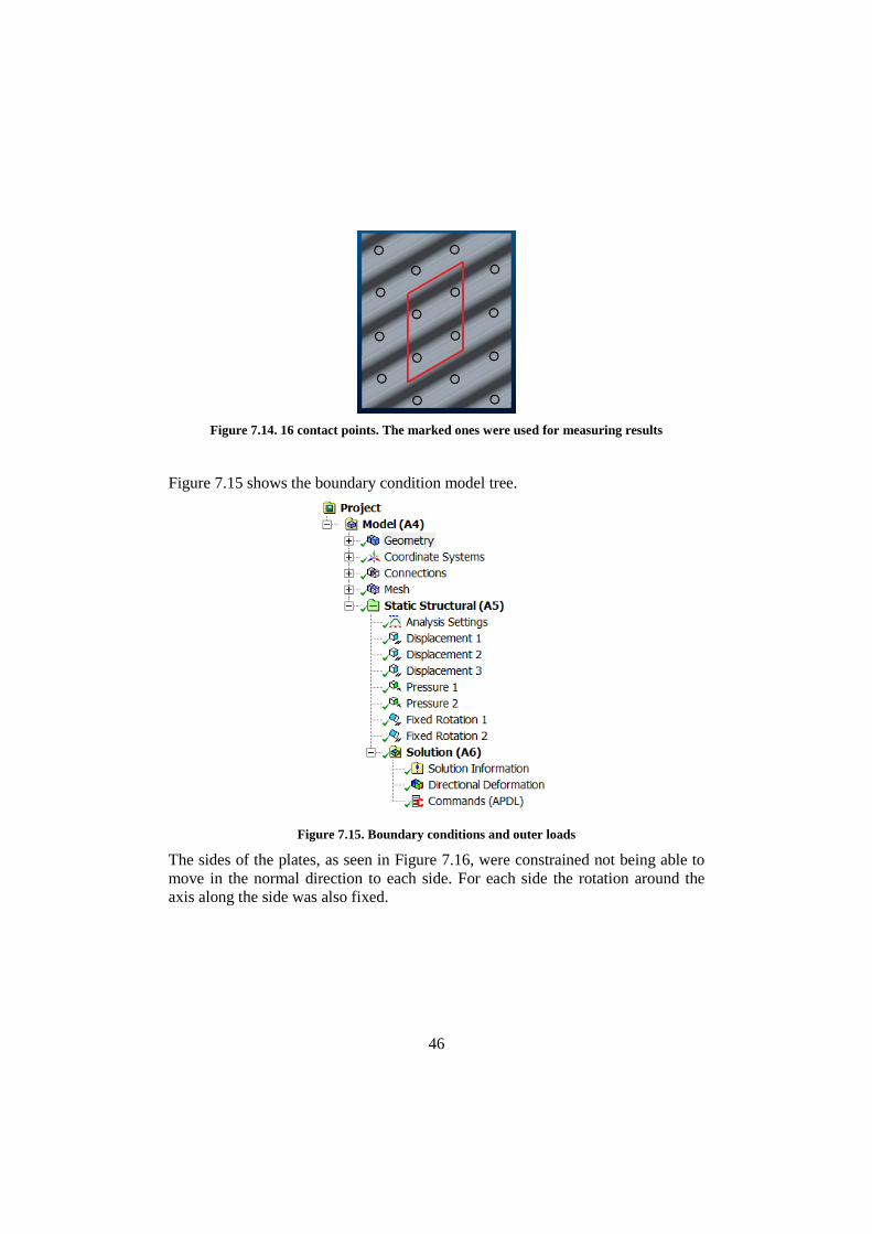
46
Figure 7.14. 16 contact points. The marked ones were used for measuring results
Figure 7.15 shows the boundary condition model tree.
Figure 7.15. Boundary conditions and outer loads
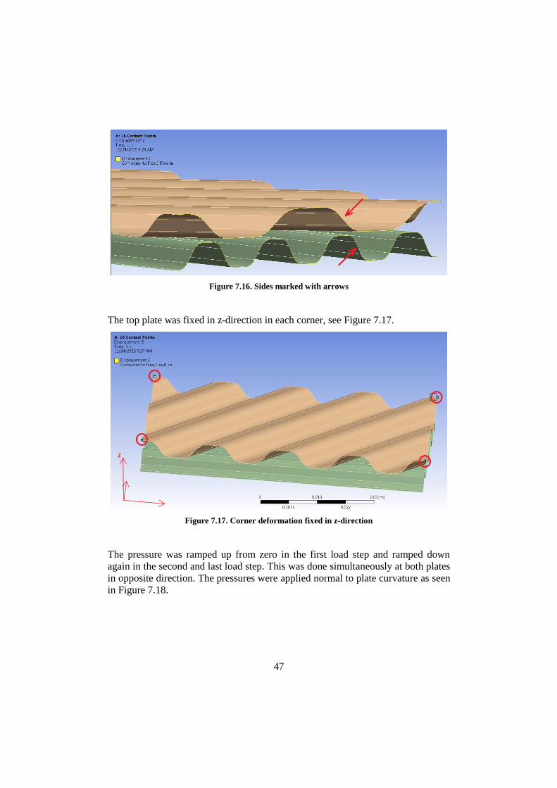
The sides of the plates, as seen in Figure 7.16, were constrained not being able to
move in the normal direction to each side. For each side the rotation around the
axis along the side was also fixed.
47
Figure 7.16. Sides marked with arrows
The top plate was fixed in z-direction in each corner, see Figure 7.17.
Figure 7.17. Corner deformation fixed in z-direction
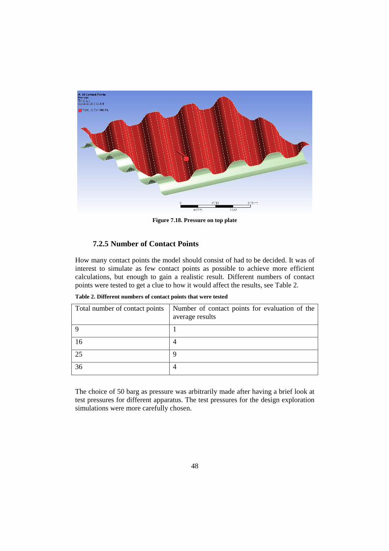
The pressure was ramped up from zero in the first load step and ramped down
again in the second and last load step. This was done simultaneously at both plates
in opposite direction. The pressures were applied normal to plate curvature as seen
in Figure 7.18.
z
48
Figure 7.18. Pressure on top plate
7.2.5 Number of Contact Points
How many contact points the model should consist of had to be decided. It was of
interest to simulate as few contact points as possible to achieve more efficient
calculations, but enough to gain a realistic result. Different numbers of contact
points were tested to get a clue to how it would affect the results, see Table 2.
Table 2. Different numbers of contact points that were tested
Total number of contact points Number of contact points for evaluation of the
average results
9 1
16 4
25 9
36 4
The choice of 50 barg as pressure was arbitrarily made after having a brief look at
test pressures for different apparatus. The test pressures for the design exploration
simulations were more carefully chosen.
49
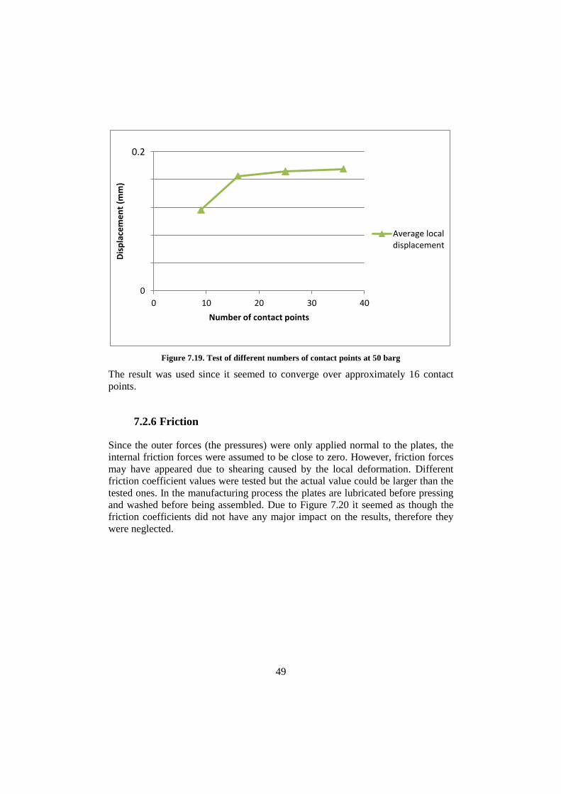
Figure 7.19. Test of different numbers of contact points at 50 barg
The result was used since it seemed to converge over approximately 16 contact
points.
7.2.6 Friction
Since the outer forces (the pressures) were only applied normal to the plates, the
internal friction forces were assumed to be close to zero. However, friction forces
may have appeared due to shearing caused by the local deformation. Different
friction coefficient values were tested but the actual value could be larger than the
tested ones. In the manufacturing process the plates are lubricated before pressing
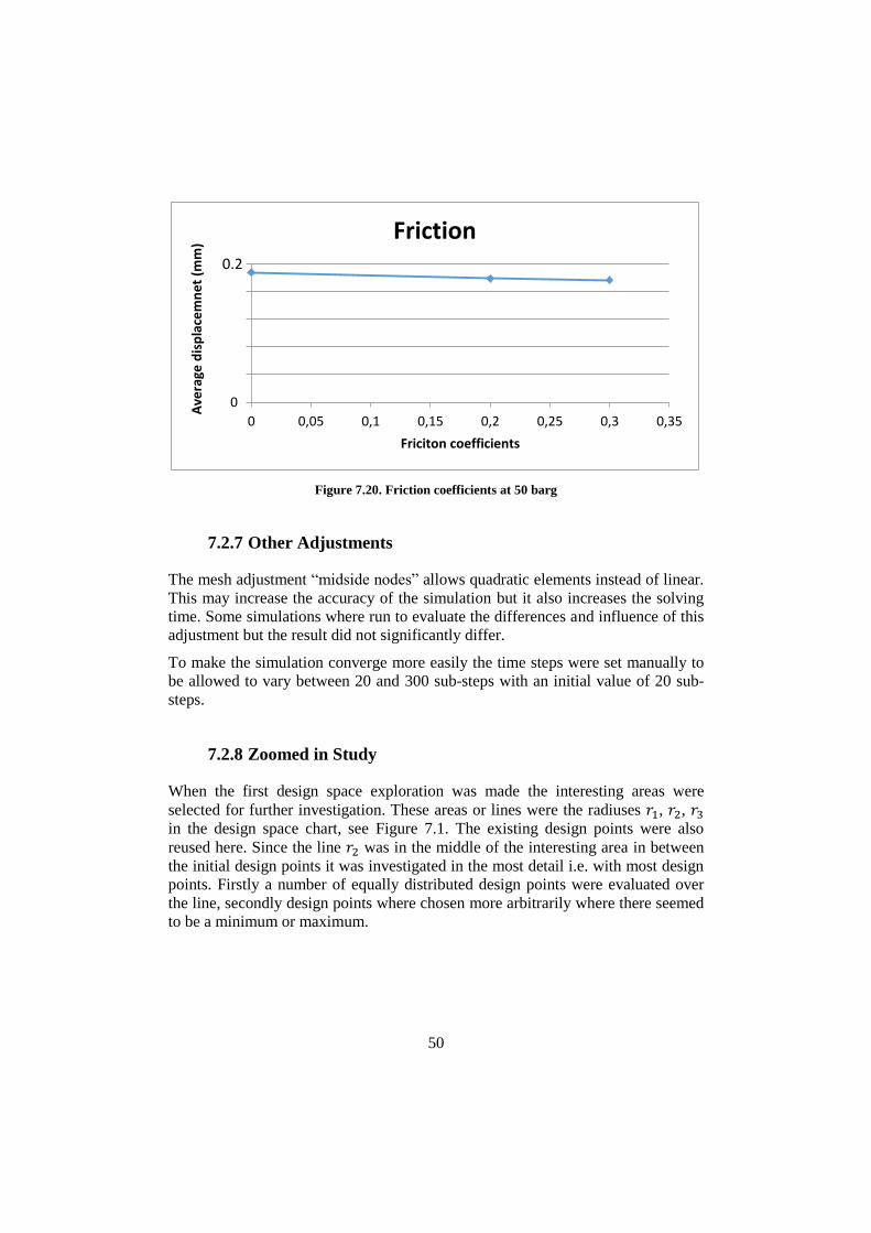
and washed before being assembled. Due to Figure 7.20 it seemed as though the
friction coefficients did not have any major impact on the results, therefore they
were neglected.
0
0,05
0,1
0,15
0,2
0,25
0 10 20 30 40
Dis
pla
cem
en
t (m
m)
Number of contact points
Average localdisplacement
0.2
50
Figure 7.20. Friction coefficients at 50 barg
7.2.7 Other Adjustments
The mesh adjustment “midside nodes” allows quadratic elements instead of linear.
This may increase the accuracy of the simulation but it also increases the solving
time. Some simulations where run to evaluate the differences and influence of this
adjustment but the result did not significantly differ.
To make the simulation converge more easily the time steps were set manually to
be allowed to vary between 20 and 300 sub-steps with an initial value of 20 sub-
steps.
7.2.8 Zoomed in Study
When the first design space exploration was made the interesting areas were
selected for further investigation. These areas or lines were the radiuses 𝑟1, 𝑟2, 𝑟3
in the design space chart, see Figure 7.1. The existing design points were also
reused here. Since the line 𝑟2 was in the middle of the interesting area in between
the initial design points it was investigated in the most detail i.e. with most design
points. Firstly a number of equally distributed design points were evaluated over
the line, secondly design points where chosen more arbitrarily where there seemed
to be a minimum or maximum.
0
0,05
0,1
0,15
0,2
0,25
0 0,05 0,1 0,15 0,2 0,25 0,3 0,35
Ave
rage
dis
pla
cem
ne
t (m
m)
Friciton coefficients
Friction 0.2
0.2
51
7.2.9 Software interference
The geometry in Creo was made to be controlled by relations based on the
previously described geometry equations. This means that the geometry could be
controlled completely by the two parameters radius and plate angle. In Ansys
workbench a test matrix was made with different parameter values. The two
different types of software were connected and the geometry could be modified for
each simulation from the test matrix in Ansys. No manual interference was
needed.
7.3 Post Process of Results
When post processing results it is preferable to make the different simulations easy
to compare and ideally find one comparable value for each test. It was possible to
measure the deformation over one single contact point, but due to local variations
the result may differ slightly over the contact points. To make the results more
reliable four contact points were measured and an average value was calculated.
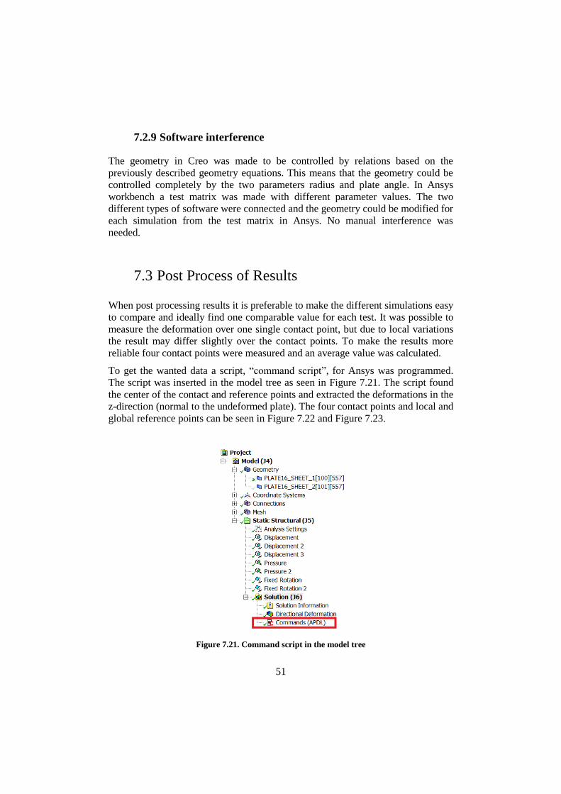
To get the wanted data a script, “command script”, for Ansys was programmed.
The script was inserted in the model tree as seen in Figure 7.21. The script found
the center of the contact and reference points and extracted the deformations in the
z-direction (normal to the undeformed plate). The four contact points and local and
global reference points can be seen in Figure 7.22 and Figure 7.23.
Figure 7.21. Command script in the model tree
52
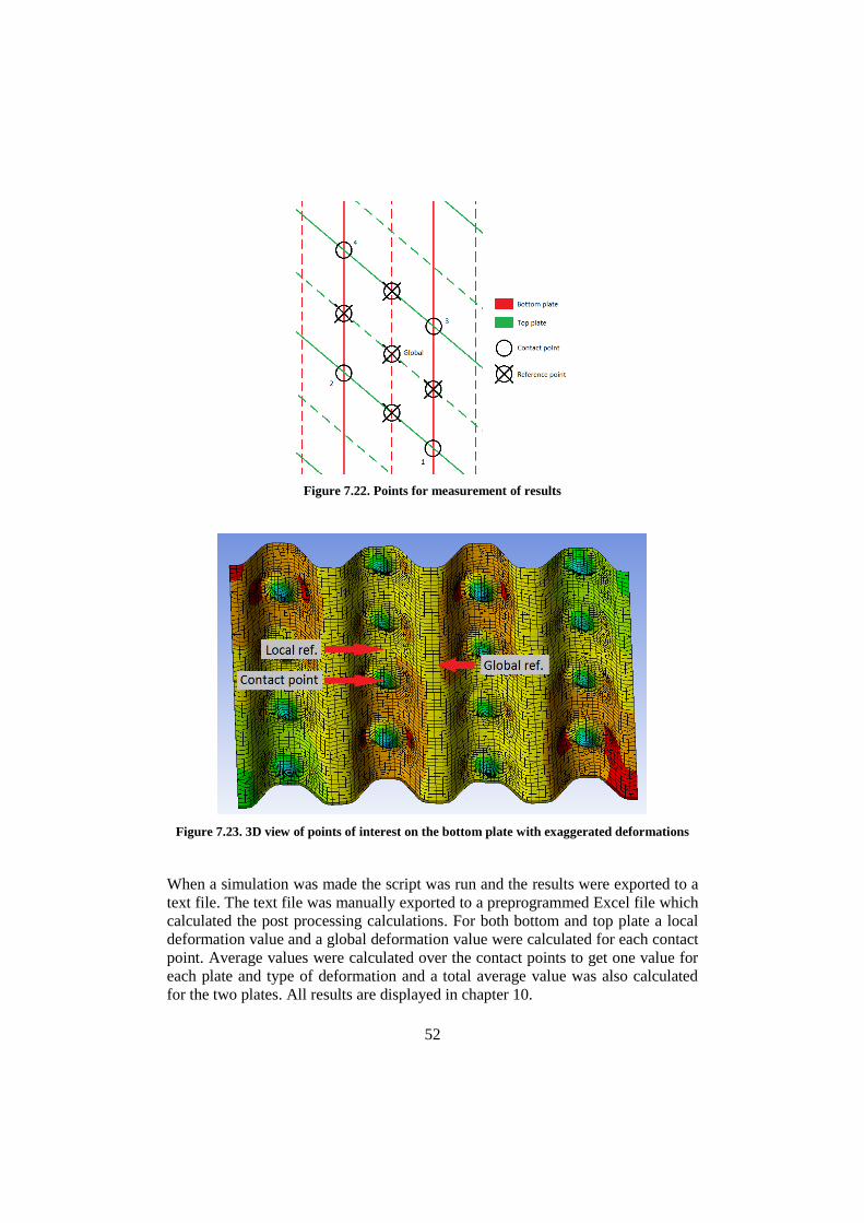
Figure 7.22. Points for measurement of results
Figure 7.23. 3D view of points of interest on the bottom plate with exaggerated deformations
When a simulation was made the script was run and the results were exported to a
text file. The text file was manually exported to a preprogrammed Excel file which
calculated the post processing calculations. For both bottom and top plate a local
deformation value and a global deformation value were calculated for each contact
point. Average values were calculated over the contact points to get one value for
each plate and type of deformation and a total average value was also calculated
for the two plates. All results are displayed in chapter 10.
53
8 Forming and Pressure Simulations
The Forming and Pressure Simulations were based on a simulation routine that
Alfa Laval uses to evaluate new plate tools and plates. This simulation routine
uses the LS-Dyna FEM solver which in this case uses an explicit solver, unlike the
implicit solver which Ansys ordinarily uses.
8.1 Purpose
The aim with these simulations was to verify or dismiss the findings from the
design space exploration simulations. This simulation method includes the plate
forming process; hence, it is more realistic. The method was not used for the
design space exploration simulations because it is much more time consuming
since each simulation has to be manually prepared for all steps from CAD to
forming and pressure simulation. Since this simulation routine is used by Alfa
Laval in development of plates it was of interest to see how the results would
differ from the other simulation model and also from reality in terms of the
laboratory experiments.
8.2 Constraints
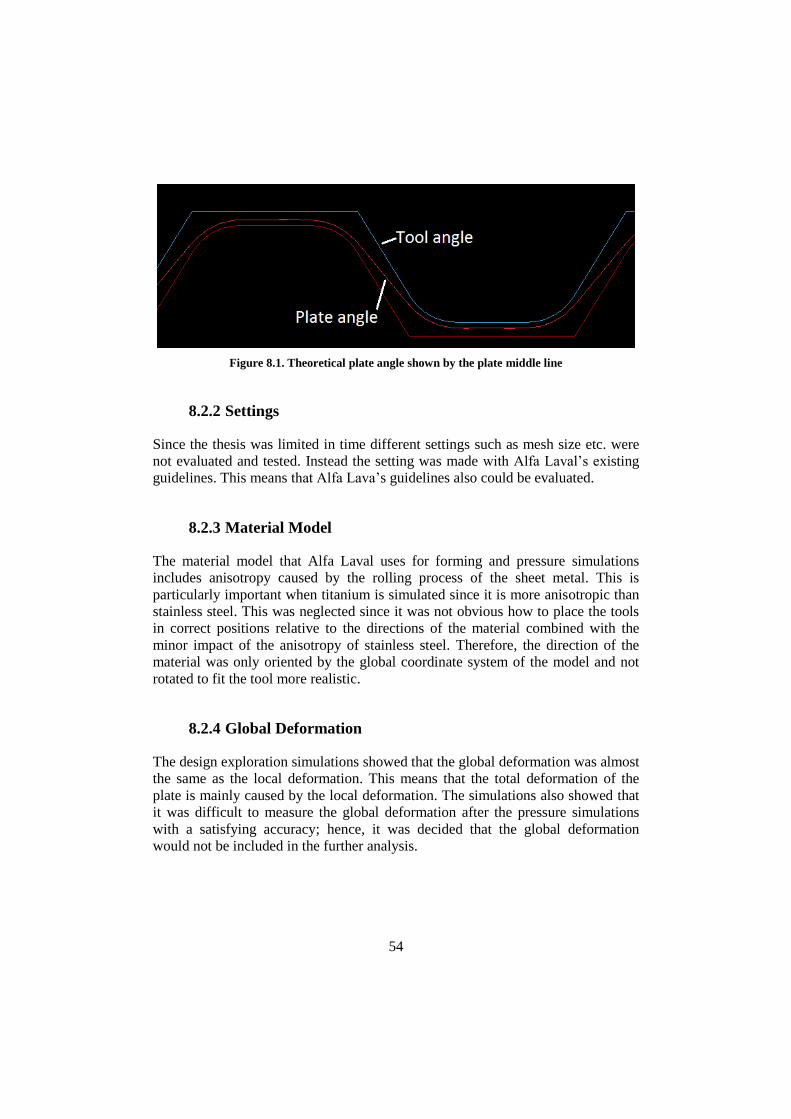
8.2.1 Theoretical Plate Angle
In the design exploration simulations the plate was directly modulated and
therefore all parameters could be controlled precisely. When the tool was
modulated instead of the plate the aim was to obtain the theoretical plate
parameters. The real values, e.g. plate angle would differ a bit since the theoretical
value assumes a homogenous, undeformed plate thickness. In reality the thickness
decreases as a consequence of the forming and this will cause a different plate
angle. The tool angle and plate angle also differs, since the tool is made to press
multiple plate thicknesses. The difference between plate angle and tool angle can
be seen in Figure 8.1.
54
Figure 8.1. Theoretical plate angle shown by the plate middle line
8.2.2 Settings
Since the thesis was limited in time different settings such as mesh size etc. were
not evaluated and tested. Instead the setting was made with Alfa Laval’s existing
guidelines. This means that Alfa Lava’s guidelines also could be evaluated.
8.2.3 Material Model
The material model that Alfa Laval uses for forming and pressure simulations
includes anisotropy caused by the rolling process of the sheet metal. This is
particularly important when titanium is simulated since it is more anisotropic than
stainless steel. This was neglected since it was not obvious how to place the tools
in correct positions relative to the directions of the material combined with the
minor impact of the anisotropy of stainless steel. Therefore, the direction of the
material was only oriented by the global coordinate system of the model and not
rotated to fit the tool more realistic.
8.2.4 Global Deformation
The design exploration simulations showed that the global deformation was almost
the same as the local deformation. This means that the total deformation of the
plate is mainly caused by the local deformation. The simulations also showed that
it was difficult to measure the global deformation after the pressure simulations
with a satisfying accuracy; hence, it was decided that the global deformation
would not be included in the further analysis.
55
8.2.5 Design Points
It was of interest to investigate the radius which was examined in most detail in
the design exploration study, i.e. 𝑟2 in Figure 7.1. The radius 𝑟3 was also of interest
to investigate since it was quite close to the radius used in the reference plate.
8.3 Simulation Model Approach
The method which was used is the same as Alfa Laval uses when developing
plates and it consists of two major steps. Firstly the plate forming simulations were
made, in this case one for each plate. Secondarily the formed plate with all internal
stresses and other information was assembled in a pressure simulation where the
plates were forced together and a pressure was applied.
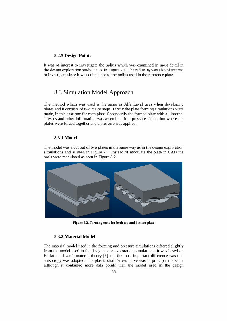
8.3.1 Model
The model was a cut out of two plates in the same way as in the design exploration
simulations and as seen in Figure 7.7. Instead of modulate the plate in CAD the
tools were modulated as seen in Figure 8.2.
Figure 8.2. Forming tools for both top and bottom plate
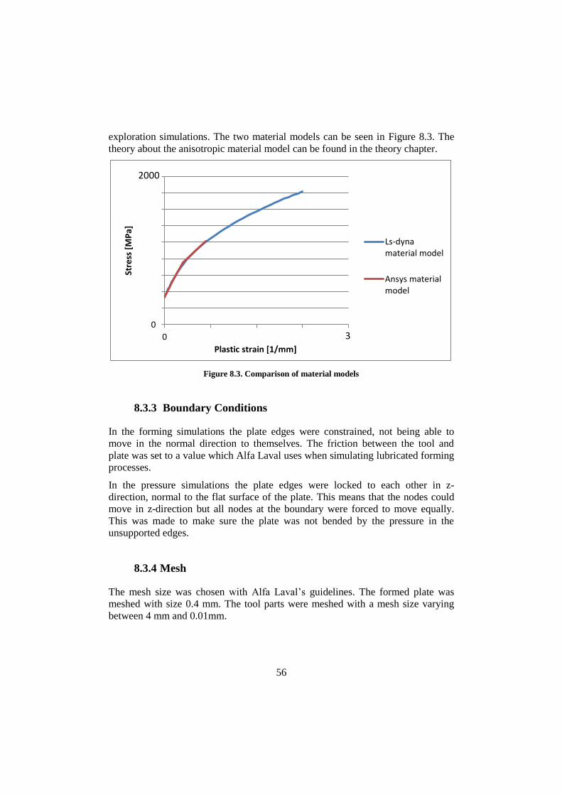
8.3.2 Material Model
The material model used in the forming and pressure simulations differed slightly
from the model used in the design space exploration simulations. It was based on
Barlat and Lean’s material theory [6] and the most important difference was that
anisotropy was adopted. The plastic strain/stress curve was in principal the same
although it contained more data points than the model used in the design
56
exploration simulations. The two material models can be seen in Figure 8.3. The
theory about the anisotropic material model can be found in the theory chapter.
Figure 8.3. Comparison of material models
8.3.3 Boundary Conditions
In the forming simulations the plate edges were constrained, not being able to
move in the normal direction to themselves. The friction between the tool and
plate was set to a value which Alfa Laval uses when simulating lubricated forming
processes.
In the pressure simulations the plate edges were locked to each other in z-
direction, normal to the flat surface of the plate. This means that the nodes could
move in z-direction but all nodes at the boundary were forced to move equally.
This was made to make sure the plate was not bended by the pressure in the
unsupported edges.
8.3.4 Mesh
The mesh size was chosen with Alfa Laval’s guidelines. The formed plate was
meshed with size 0.4 mm. The tool parts were meshed with a mesh size varying
between 4 mm and 0.01mm.
0
200
400
600
800
1000
1200
1400
1600
1800
0 0,5 1 1,5 2
Stre
ss [
MP
a]
Plastic strain [1/mm]
Ls-dynamaterial model
Ansys materialmodel
2000
3
57
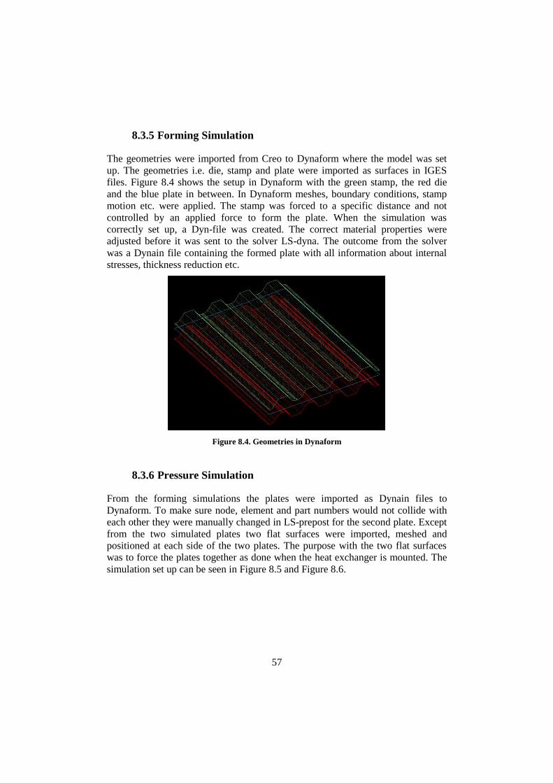
8.3.5 Forming Simulation
The geometries were imported from Creo to Dynaform where the model was set
up. The geometries i.e. die, stamp and plate were imported as surfaces in IGES
files. Figure 8.4 shows the setup in Dynaform with the green stamp, the red die
and the blue plate in between. In Dynaform meshes, boundary conditions, stamp
motion etc. were applied. The stamp was forced to a specific distance and not
controlled by an applied force to form the plate. When the simulation was
correctly set up, a Dyn-file was created. The correct material properties were
adjusted before it was sent to the solver LS-dyna. The outcome from the solver
was a Dynain file containing the formed plate with all information about internal
stresses, thickness reduction etc.
Figure 8.4. Geometries in Dynaform
8.3.6 Pressure Simulation
From the forming simulations the plates were imported as Dynain files to
Dynaform. To make sure node, element and part numbers would not collide with
each other they were manually changed in LS-prepost for the second plate. Except
from the two simulated plates two flat surfaces were imported, meshed and
positioned at each side of the two plates. The purpose with the two flat surfaces
was to force the plates together as done when the heat exchanger is mounted. The
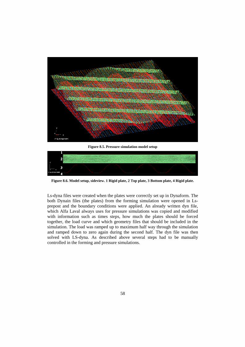
simulation set up can be seen in Figure 8.5 and Figure 8.6.
58
Figure 8.5. Pressure simulation model setup
Figure 8.6. Model setup, sideview. 1 Rigid plate, 2 Top plate, 3 Bottom plate, 4 Rigid plate.
Ls-dyna files were created when the plates were correctly set up in Dynaform. The
both Dynain files (the plates) from the forming simulation were opened in Ls-
prepost and the boundary conditions were applied. An already written dyn file,
which Alfa Laval always uses for pressure simulations was copied and modified
with information such as times steps, how much the plates should be forced
together, the load curve and which geometry files that should be included in the
simulation. The load was ramped up to maximum half way through the simulation
and ramped down to zero again during the second half. The dyn file was then
solved with LS-dyna. As described above several steps had to be manually
controlled in the forming and pressure simulations.
59
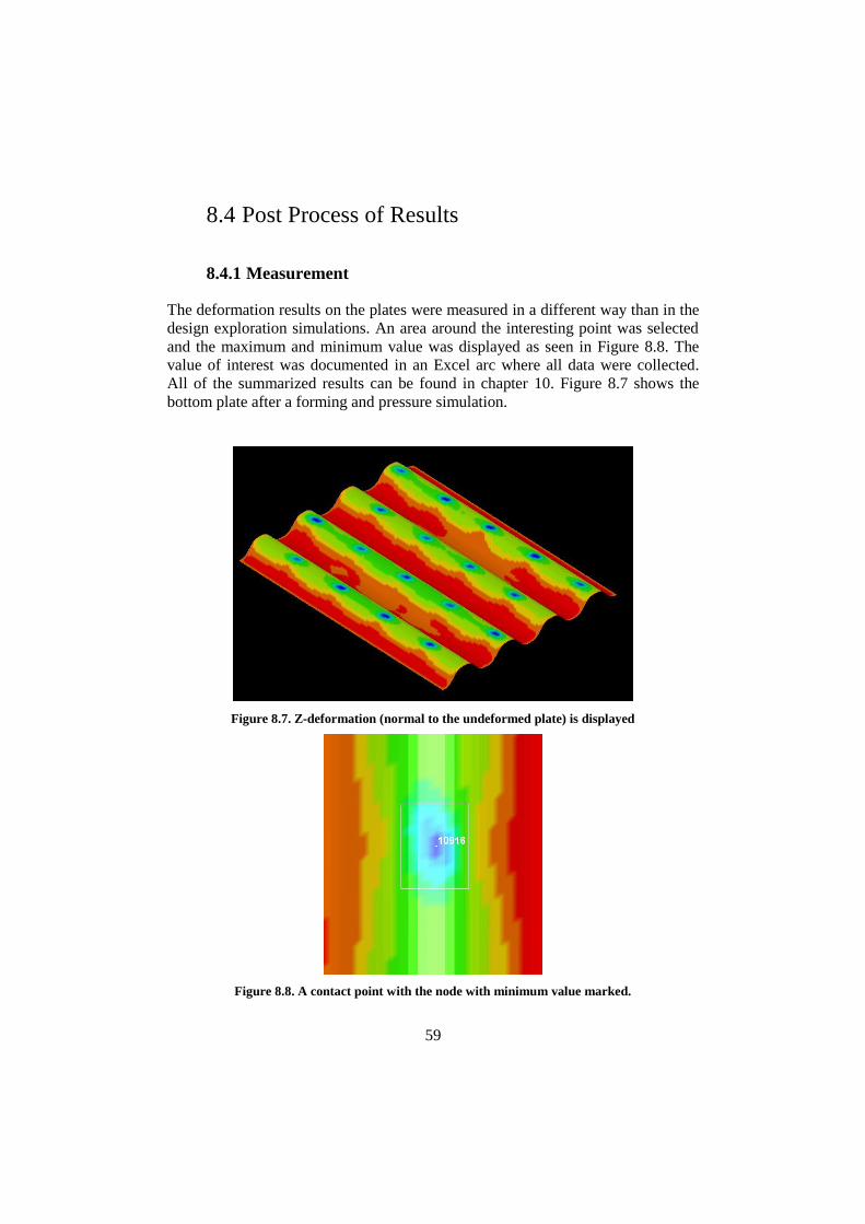
8.4 Post Process of Results
8.4.1 Measurement
The deformation results on the plates were measured in a different way than in the
design exploration simulations. An area around the interesting point was selected
and the maximum and minimum value was displayed as seen in Figure 8.8. The
value of interest was documented in an Excel arc where all data were collected.
All of the summarized results can be found in chapter 10. Figure 8.7 shows the
bottom plate after a forming and pressure simulation.
Figure 8.7. Z-deformation (normal to the undeformed plate) is displayed
Figure 8.8. A contact point with the node with minimum value marked.

61
9 Laboratory Experiments
To know if the simulated models were realistic and reliable they were verified by
examining the reference plate. A description how it was made by laboratory
experiments follows.
9.1 Constraints
Two different plate thicknesses were tested, 0.4 mm and 0.5 mm, to make sure that
the models were independent of the plate thickness. The experiments were limited
to four pressure levels for each plate thickness, i.e. totally eight tests were
performed. An attempt to measure the global deformations was made but since it
was difficult to measure them with a satisfying accuracy they were not included in
the analysis. Instead only the local deformations were analyzed.
9.2 Experimental Approach
Different pressure levels were applied and the deformations were examined at
each level. After a test with a certain pressure had been run the plates were
replaced with new plates for next pressure level. The first test of each plate
thickness was first assembled with an extra plate which was taken out before the
pressurization. These extra plates were references to see if any deformations
occurred due to the forces from the assembly process.
9.2.1 Pressure Levels
Different pressures were used in the tests to make sure that the simulations follow
the reality through all time/pressure steps. It was important to make sure the tested
pressures gave remaining deformations. To decide which pressures to use the
maximum allowed test pressure was tried first. Note that the maximum allowed
test pressure is decided with safety factors, which means that the proved actual
leakage pressure is higher. After the first tests the PHE was disassembled and the
plates were examined ocularly. The deformations were considered to be moderate,
62
i.e. they were visible but it was estimated that they were far from fracture. With
this in mind the rest of the pressure levels were chosen. Since the deformations
were considered moderate one test level with lower pressure and two with higher
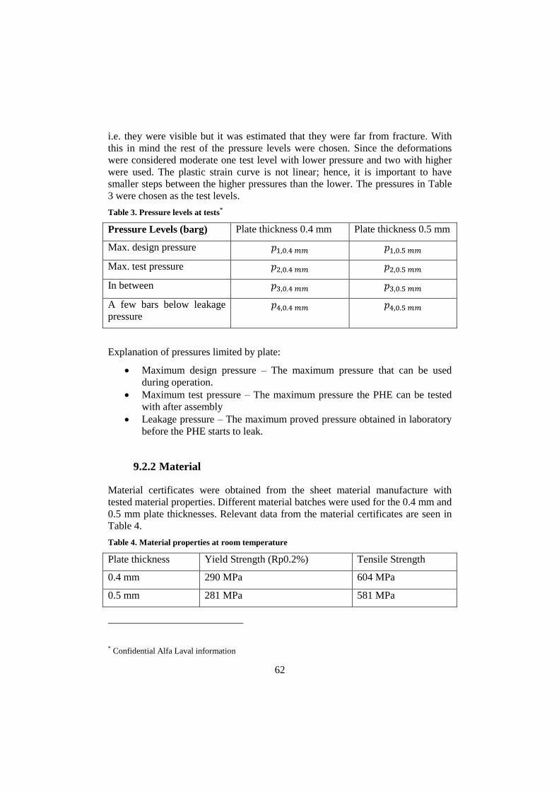
were used. The plastic strain curve is not linear; hence, it is important to have
smaller steps between the higher pressures than the lower. The pressures in Table
3 were chosen as the test levels.
Table 3. Pressure levels at tests*
Pressure Levels (barg) Plate thickness 0.4 mm Plate thickness 0.5 mm
Max. design pressure 𝑝1,0.4 𝑚𝑚 𝑝1,0.5 𝑚𝑚
Max. test pressure 𝑝2,0.4 𝑚𝑚 𝑝2,0.5 𝑚𝑚
In between 𝑝3,0.4 𝑚𝑚 𝑝3,0.5 𝑚𝑚
A few bars below leakage
pressure 𝑝4,0.4 𝑚𝑚 𝑝4,0.5 𝑚𝑚
Explanation of pressures limited by plate:
Maximum design pressure – The maximum pressure that can be used
during operation.
Maximum test pressure – The maximum pressure the PHE can be tested
with after assembly
Leakage pressure – The maximum proved pressure obtained in laboratory
before the PHE starts to leak.
9.2.2 Material
Material certificates were obtained from the sheet material manufacture with
tested material properties. Different material batches were used for the 0.4 mm and
0.5 mm plate thicknesses. Relevant data from the material certificates are seen in
Table 4.
Table 4. Material properties at room temperature
Plate thickness Yield Strength (Rp0.2%) Tensile Strength
0.4 mm 290 MPa 604 MPa
0.5 mm 281 MPa 581 MPa
* Confidential Alfa Laval information
63
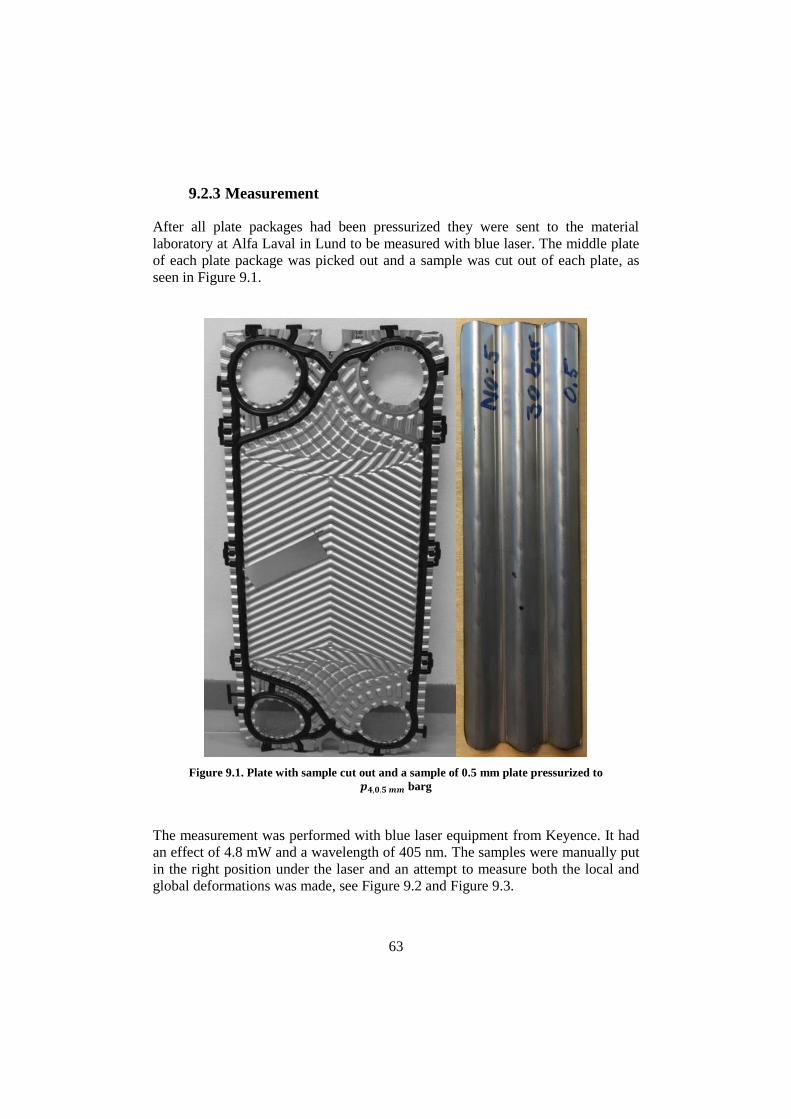
9.2.3 Measurement
After all plate packages had been pressurized they were sent to the material
laboratory at Alfa Laval in Lund to be measured with blue laser. The middle plate
of each plate package was picked out and a sample was cut out of each plate, as
seen in Figure 9.1.
Figure 9.1. Plate with sample cut out and a sample of 0.5 mm plate pressurized to 𝒑𝟒,𝟎.𝟓 𝒎𝒎 barg
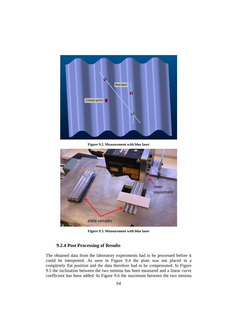
The measurement was performed with blue laser equipment from Keyence. It had
an effect of 4.8 mW and a wavelength of 405 nm. The samples were manually put
in the right position under the laser and an attempt to measure both the local and
global deformations was made, see Figure 9.2 and Figure 9.3.
64
Figure 9.2. Measurement with blue laser
Figure 9.3. Measurement with blue laser
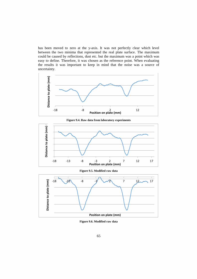
9.2.4 Post Processing of Results
The obtained data from the laboratory experiments had to be processed before it
could be interpreted. As seen in Figure 9.4 the plate was not placed in a
completely flat position and the data therefore had to be compensated. In Figure
9.5 the inclination between the two minima has been measured and a linear curve
coefficient has been added. In Figure 9.6 the maximum between the two minima
plate samples
laser equipment
65
has been moved to zero at the y-axis. It was not perfectly clear which level
between the two minima that represented the real plate surface. The maximum
could be caused by reflections, dust etc. but the maximum was a point which was
easy to define. Therefore, it was chosen as the reference point. When evaluating
the results it was important to keep in mind that the noise was a source of
uncertainty.
Figure 9.4. Raw data from laboratory experiments
Figure 9.5. Modified raw data
Figure 9.6. Modified raw data
-18 -8 2 12
Dis
tan
ce t
o p
late
(m
m)
Position on plate (mm)
5,06
5,08
5,1
5,12
5,14
5,16
-18 -13 -8 -3 2 7 12 17
Dis
tan
ce t
o p
late
(m
m)
Position on plate (mm)
-18 -13 -8 -3 2 7 12 17
Dis
tan
ce t
o p
late
(m
m)
Position on plate (mm)
66
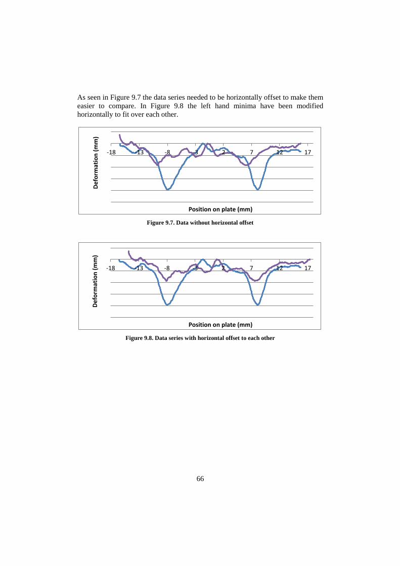
As seen in Figure 9.7 the data series needed to be horizontally offset to make them
easier to compare. In Figure 9.8 the left hand minima have been modified
horizontally to fit over each other.
Figure 9.7. Data without horizontal offset
Figure 9.8. Data series with horizontal offset to each other
-18 -13 -8 -3 2 7 12 17
De
form
atio
n (
mm
)
Position on plate (mm)
-18 -13 -8 -3 2 7 12 17
De
form
atio
n (
mm
)
Position on plate (mm)
67
10 Results
All the results are shown in this chapter. First each section is displayed separately
and finally the results are compared to each other.
10.1 Design Space Exploration
The results are analyzed and discussed in chapter 11.
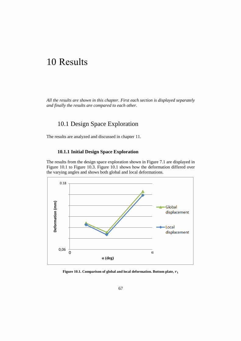
10.1.1 Initial Design Space Exploration
The results from the design space exploration shown in Figure 7.1 are displayed in
Figure 10.1 to Figure 10.3. Figure 10.1 shows how the deformation differed over
the varying angles and shows both global and local deformations.
Figure 10.1. Comparison of global and local deformation. Bottom plate, 𝒓𝟏
0,06
0,07
0,08
0,09
0,1
0,11
0,12
De
form
atio
n (
mm
)
α (deg)
Globaldisplacement
α 0
0.18
68
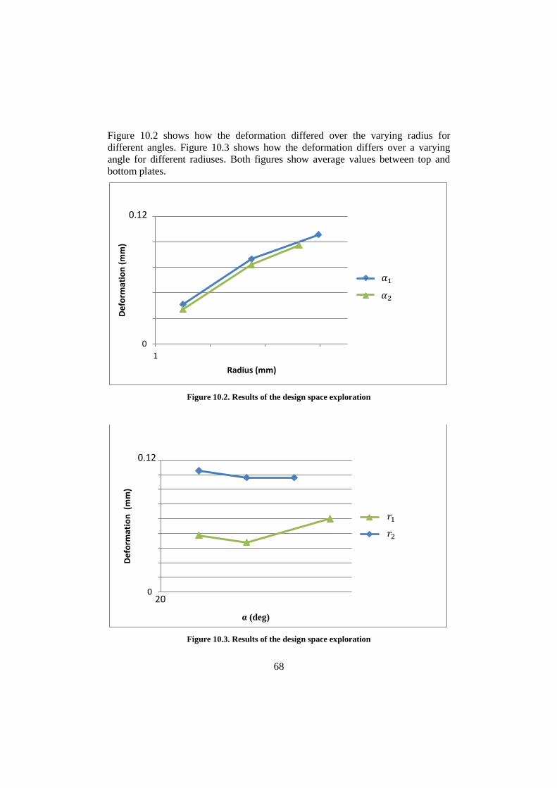
Figure 10.2 shows how the deformation differed over the varying radius for
different angles. Figure 10.3 shows how the deformation differs over a varying
angle for different radiuses. Both figures show average values between top and
bottom plates.
Figure 10.2. Results of the design space exploration
Figure 10.3. Results of the design space exploration
0
0,05
0,1
0,15
0,2
0,25
1 2 3 4
De
form
atio
n (
mm
)
Radius (mm)
α = 35 deg
α = 41.25 deg
𝛼1
𝛼2
0.12
0
0,02
0,04
0,06
0,08
0,1
0,12
0,14
0,16
0,18
De
form
atio
n (
mm
)
α (deg)
r = 1.5 mm
r = 2.75 mm
20
0.12
𝑟1
𝑟2
69
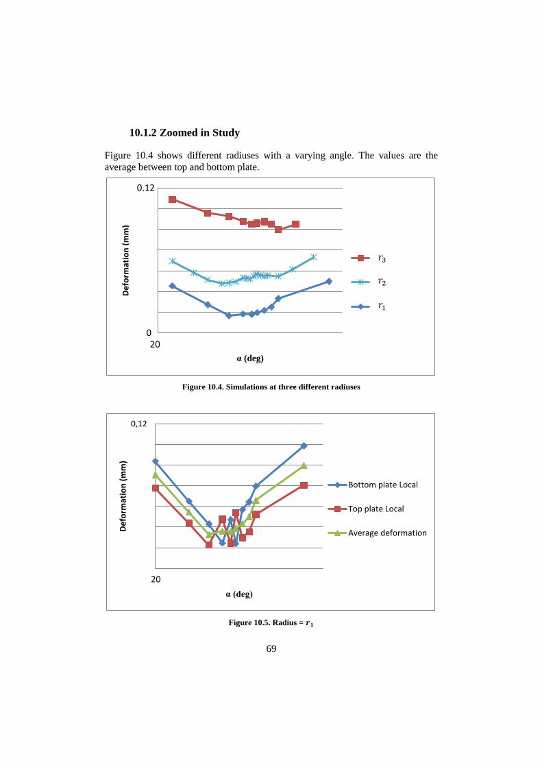
10.1.2 Zoomed in Study
Figure 10.4 shows different radiuses with a varying angle. The values are the
average between top and bottom plate.
Figure 10.4. Simulations at three different radiuses
Figure 10.5. Radius = 𝒓𝟏
0,05
0,07
0,09
0,11
0,13
0,15
0,17
0,19
28 32 36 40 44 48 52
De
form
atio
n (
mm
)
α (deg)
radius = 2.75mm
radius = 2 mm
radius = 1.5 mm
𝑟3
𝑟2 𝑟1
20
0.12
0
0,05
0,06
0,07
0,08
0,09
0,1
0,11
0,12
30 40 50
De
form
atio
n (
mm
)
α (deg)
Bottom plate Local
Top plate Local
Average deformation
20
70
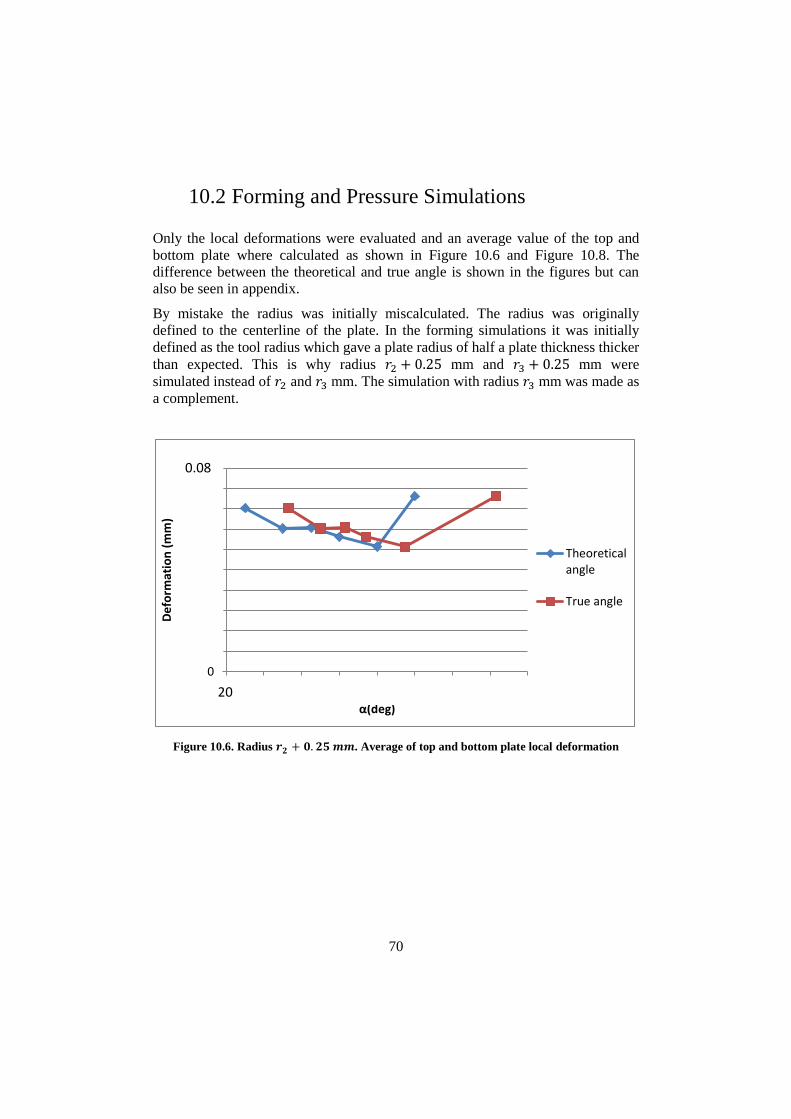
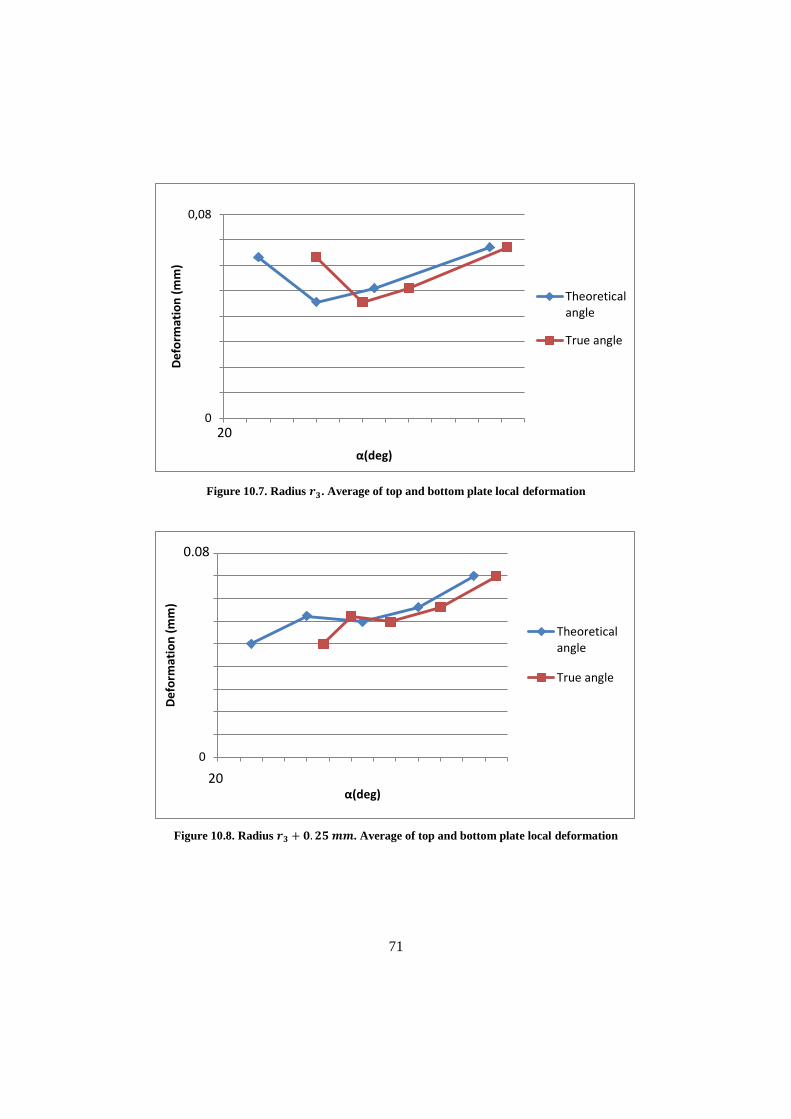
10.2 Forming and Pressure Simulations
Only the local deformations were evaluated and an average value of the top and
bottom plate where calculated as shown in Figure 10.6 and Figure 10.8. The
difference between the theoretical and true angle is shown in the figures but can
also be seen in appendix.
By mistake the radius was initially miscalculated. The radius was originally
defined to the centerline of the plate. In the forming simulations it was initially
defined as the tool radius which gave a plate radius of half a plate thickness thicker
than expected. This is why radius 𝑟2 + 0.25 mm and 𝑟3 + 0.25 mm were
simulated instead of 𝑟2 and 𝑟3 mm. The simulation with radius 𝑟3 mm was made as
a complement.
Figure 10.6. Radius 𝒓𝟐 + 𝟎. 𝟐𝟓 𝒎𝒎. Average of top and bottom plate local deformation
0
0,005
0,01
0,015
0,02
0,025
0,03
0,035
0,04
0,045
0,05
32 34 36 38 40 42 44 46 48
De
form
atio
n (
mm
)
α(deg)
Theoreticalangle
True angle
0.08
20
71
Figure 10.7. Radius 𝒓𝟑. Average of top and bottom plate local deformation
Figure 10.8. Radius 𝒓𝟑 + 𝟎. 𝟐𝟓 𝒎𝒎. Average of top and bottom plate local deformation
0
0,01
0,02
0,03
0,04
0,05
0,06
0,07
0,08
22 24 26 28 30 32 34 36 38 40 42 44 46 48
De
form
atio
n (
mm
)
α(deg)
Theoreticalangle
True angle
20
0
0,01
0,02
0,03
0,04
0,05
0,06
0,07
0,08
0,09
22 24 26 28 30 32 34 36 38 40 42 44 46 48
De
form
atio
n (
mm
)
α(deg)
Theoreticalangle
True angle
20
0.08
72
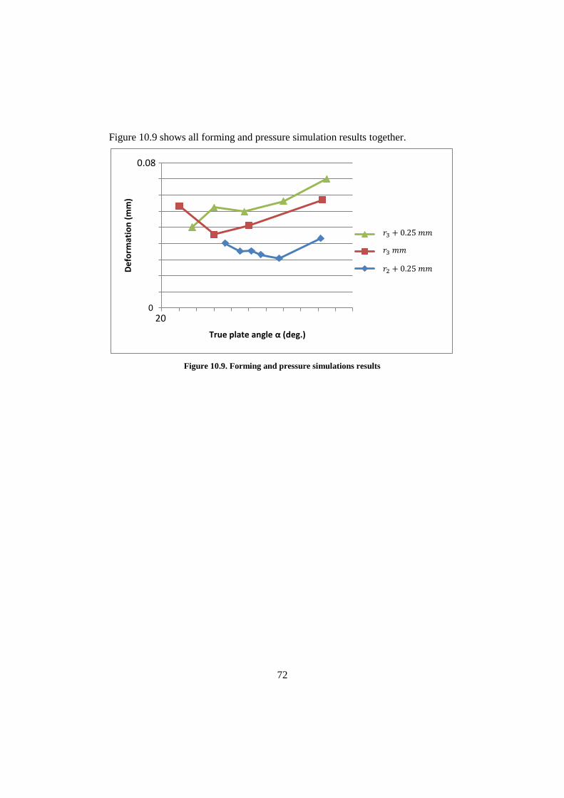
Figure 10.9 shows all forming and pressure simulation results together.
Figure 10.9. Forming and pressure simulations results
0
0,01
0,02
0,03
0,04
0,05
0,06
0,07
0,08
0,09
28 30 32 34 36 38 40 42 44 46 48 50
De
form
atio
n (
mm
)
True plate angle α (deg.)
radius = 3 mm
radius = 2.75 mm
radius = 2.25 mm
𝑟3 + 0.25 𝑚𝑚
𝑟3 𝑚𝑚
𝑟2 + 0.25 𝑚𝑚
20
0.08
73
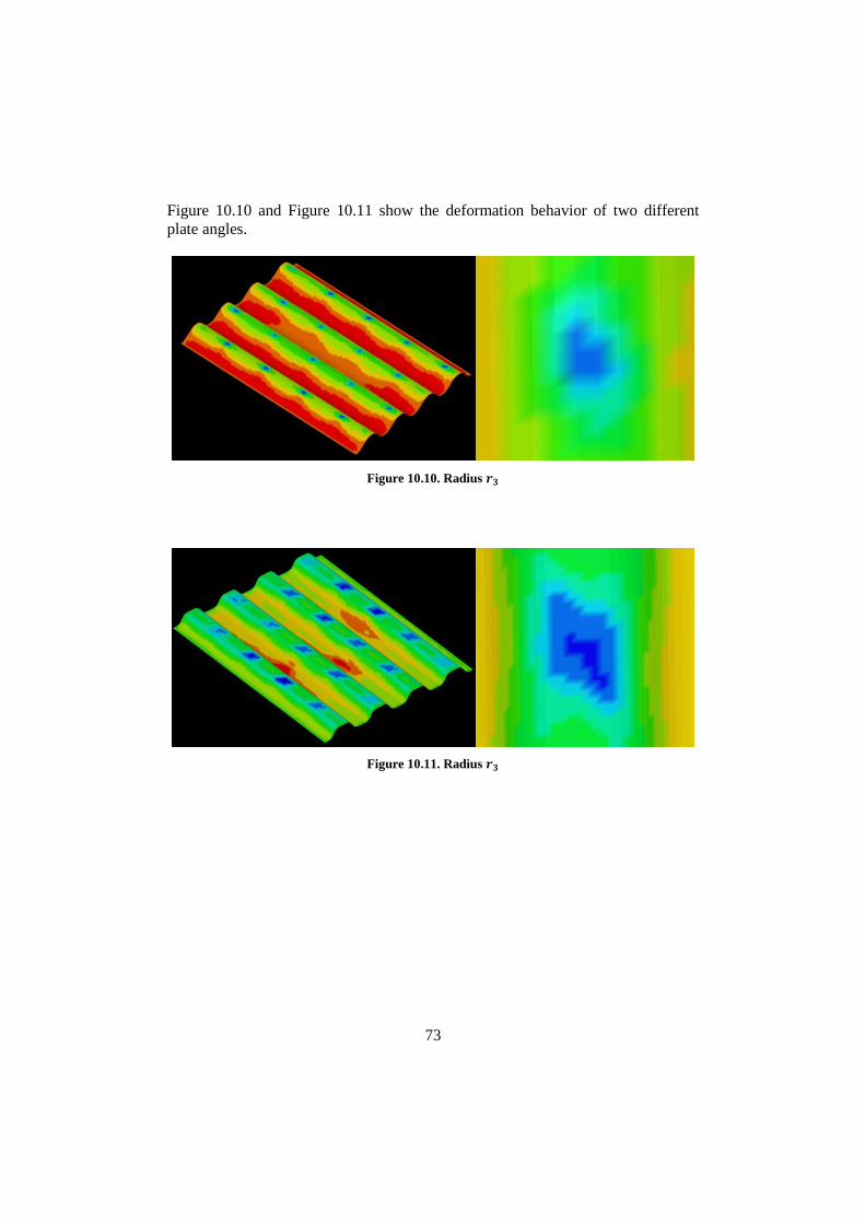
Figure 10.10 and Figure 10.11 show the deformation behavior of two different
plate angles.
Figure 10.10. Radius 𝒓𝟑
Figure 10.11. Radius 𝒓𝟑
74
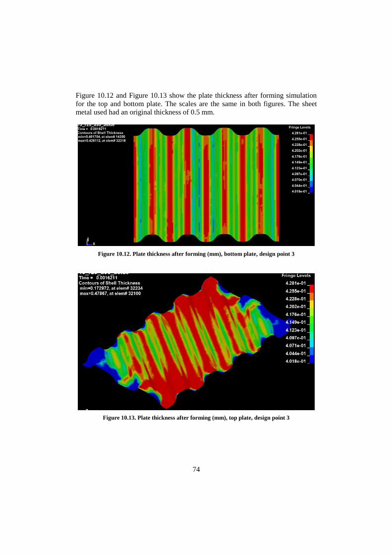
Figure 10.12 and Figure 10.13 show the plate thickness after forming simulation
for the top and bottom plate. The scales are the same in both figures. The sheet
metal used had an original thickness of 0.5 mm.
Figure 10.12. Plate thickness after forming (mm), bottom plate, design point 3
Figure 10.13. Plate thickness after forming (mm), top plate, design point 3
75
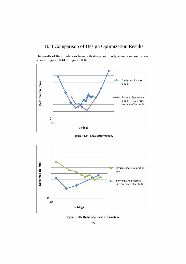
10.3 Comparison of Design Optimization Results
The results of the simulations from both Ansys and Ls-dyna are compared to each
other in Figure 10.14 to Figure 10.16.
Figure 10.14. Local deformation.
Figure 10.15. Radius 𝒓𝟑. Local deformation.
0,09
0,095
0,1
0,105
0,11
0,115
0,12
0,125
28 30 32 34 36 38 40 42 44 46 48 50 52
De
form
atio
n (
mm
)
α (deg)
Design explorationsim. r = 2 mm
Forming & pressuresim. r = 2.25 mm.Vertical offset0.065mm
0
20
Design exploration sim. 𝑟2
Forming & pressure sim. 𝑟2 + 0.25 𝑚𝑚. Vertical offset to fit
0,12
0,13
0,14
0,15
0,16
0,17
0,18
0,19
0,2
28 30 32 34 36 38 40 42 44 46 48 50
De
form
atio
n (
mm
)
α (deg)
Design explorationsim.
Froming and pressuresim. Vert. Offset 0.09mm
Forming and pressure sim. Vertical offset to fit
20 0
Design space exploration sim.
76
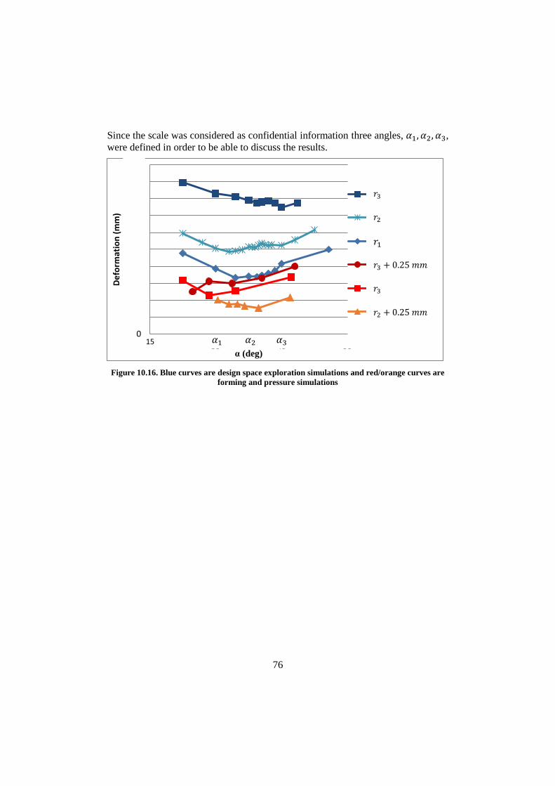
Since the scale was considered as confidential information three angles, 𝛼1, 𝛼2, 𝛼3,
were defined in order to be able to discuss the results.
Figure 10.16. Blue curves are design space exploration simulations and red/orange curves are
forming and pressure simulations
0
0,02
0,04
0,06
0,08
0,1
0,12
0,14
0,16
0,18
0,2
25 35 45 55
De
form
atio
n (
mm
)
α (deg)
Radius = 2.75 mm
Radius = 2 mm
Radius = 1.5 mm
Radius = 3 mm
Radius = 2.75 mm
Radius = 2.25 mm
𝑟3
𝑟2
𝑟1 𝑟3 + 0.25 𝑚𝑚
𝑟3
𝑟2 + 0.25 𝑚𝑚
15 𝛼1 𝛼2 𝛼3
77
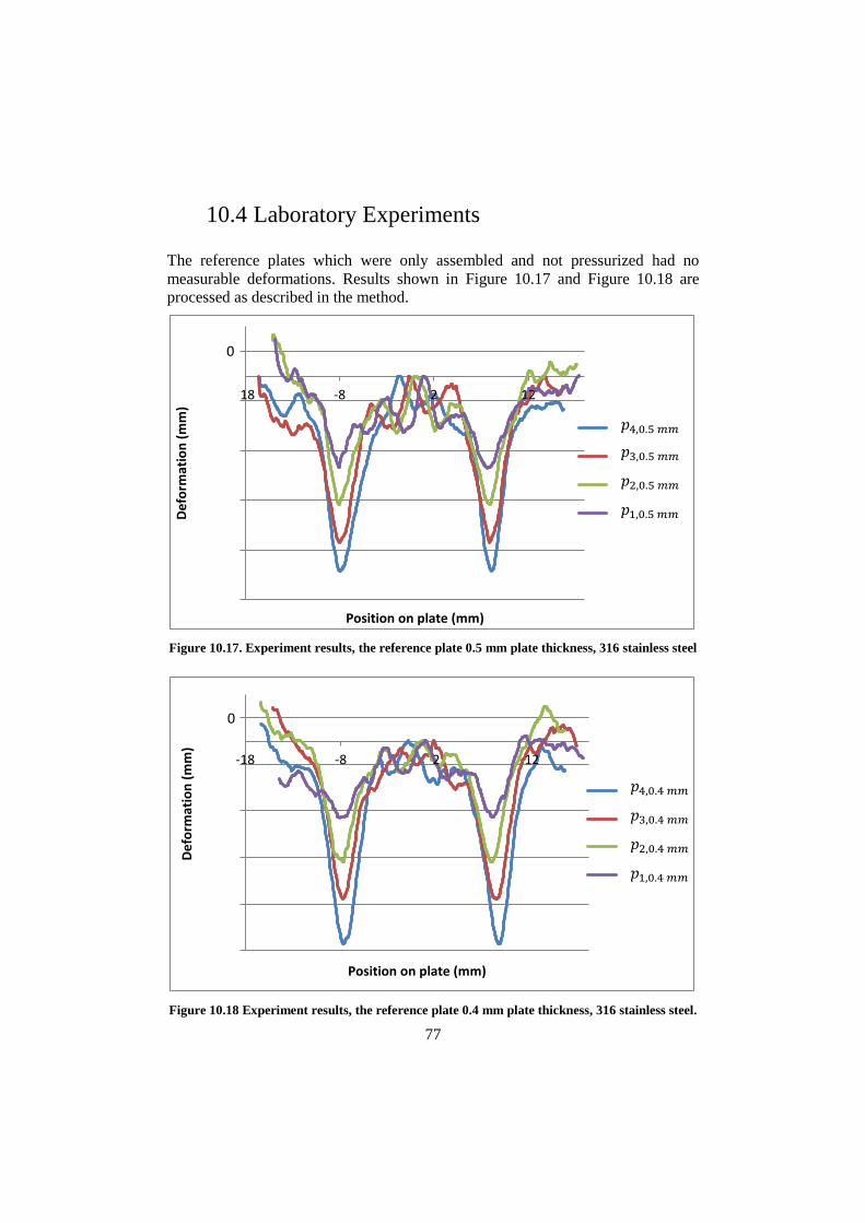
10.4 Laboratory Experiments
The reference plates which were only assembled and not pressurized had no
measurable deformations. Results shown in Figure 10.17 and Figure 10.18 are
processed as described in the method.
Figure 10.17. Experiment results, the reference plate 0.5 mm plate thickness, 316 stainless steel
Figure 10.18 Experiment results, the reference plate 0.4 mm plate thickness, 316 stainless steel.
-0,09
-0,07
-0,05
-0,03
-0,01
0,01
-18 -8 2 12
De
form
atio
n (
mm
)
Position on plate (mm)
30 bar
26.5 bar
23 bar
18 bar
𝑝4,0.5 𝑚𝑚
𝑝3,0.5 𝑚𝑚
𝑝2,0.5 𝑚𝑚
𝑝1,0.5 𝑚𝑚
0
-0,09
-0,07
-0,05
-0,03
-0,01
0,01
-18 -8 2 12
De
form
atio
n (
mm
)
Position on plate (mm)
21 bar
18,5 bar
16 bar
12 bar
𝑝4,0.4 𝑚𝑚
𝑝3,0.4 𝑚𝑚
𝑝2,0.4 𝑚𝑚
𝑝1,0.4 𝑚𝑚
0
78
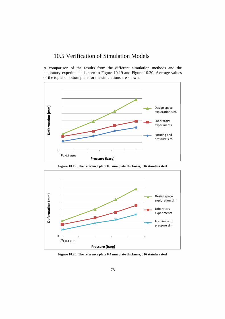
10.5 Verification of Simulation Models
A comparison of the results from the different simulation methods and the
laboratory experiments is seen in Figure 10.19 and Figure 10.20. Average values
of the top and bottom plate for the simulations are shown.
Figure 10.19. The reference plate 0.5 mm plate thickness, 316 stainless steel
Figure 10.20. The reference plate 0.4 mm plate thickness, 316 stainless steel
0
0,02
0,04
0,06
0,08
0,1
0,12
0,14
0,16
18 20 22 24 26 28 30
De
form
atio
n [
mm
]
Pressure (barg)
Ansys
Lab. Experiments
LS-dyna
𝑝1,0.5 𝑚𝑚
Design space exploration sim.
Laboratory experiments
Forming and pressure sim.
0
0,02
0,04
0,06
0,08
0,1
0,12
0,14
0,16
12 14 16 18 20 22
De
form
atio
n (
mm
)
Pressure (barg)
Ansys
Lab. Experiments
Ls-dyna
𝑝1,0.4 𝑚𝑚
Design space exploration sim. Laboratory experiments Forming and pressure sim.
79
11 Discussion
The following chapter discusses the results and which improvements that could
have been made. The conclusions of the thesis are also gathered.
11.1 Design Exploration Simulations
The aim of the design exploration simulation model was not to get perfect results
but to get a brief picture of the design space. It was already known that the
simplifications were considerable and that it would make the result differ
significantly from the reality. The expectations were rather to see if any geometry
dependencies could be found and if these trends, despite their absolute values,
would correspond to more precise calculation models or to reality. It was
considerably easier to run a large amount of simulations with this model than the
forming and pressure simulation model, which was a great benefit.
Two obvious effects as a result of the neglected forming procedure were
identified. When a plate is formed it becomes thinner, but not homogenously
thinner as it was modulated in this model. The thinning occurs more locally as
seen in Figure 10.12 and Figure 10.13. The inhomogeneous thickness affect
should have an impact on the results, but it was not completely clear if the affect
should make the deformations greater or smaller. Another aspect which was not
considered is the hardening of the metal which occurs when the plates are cold
formed. The hardening affect should have made the deformations smaller if they
were considered.
It is seen in Figure 10.1 that the differences between global and local deformations
were next to none. This was seen in all of the design exploration simulations. Yet,
the global deformations were slightly greater than the local deformations, which
indicate that there might occur more deformations than just the local ones. Since it
looks like the local deformation accounts for the major part of the deformation
together with the fact that it was hard to measure the global deformation properly,
the global deformations were not included in the further analysis. An investigation
about the impact of the global deformation has been noted as a possible future
improvement. The effect from the unevenly distributed plate thinning may
increase or decrease the difference between global and local deformation.
80
Figure 10.5 shows the local deformation for top and bottom plate with a 𝑟1 radius.
It can be seen that there is a difference between top and bottom plate and that there
are notches on the two curves. It seems like the values between top and bottom
plate for some design points have changed places. Though the reason for this is not
clear, it is probably caused by unidentified of instabilities in the model. When an
average of top and bottom plate was calculated the resultant curve looked more
correct, which can be seen in Figure 10.4. One contributing reason for this can be
that the top plate was constrained in each corner unlike the bottom plate. Another
reason can be the way the upper plate was cut in an angle with a different
boundary compared to the bottom plate. However, as long as the two plates show
the same trend, the vertical offset in the figure is a minor problem.
11.2 Forming and Pressure Simulations
The anisotropic material model was directly adopted from Alfa Laval’s forming
and pressure simulation procedure. The direction of the material was not adjusted
to fit the model which has been a source of error, although it was considered to be
of minor importance since stainless steel is an isotropic material unlike e.g.
titanium. It may have contributed to the difference between upper and lower plate
since they were oriented differently in relation to the material model. This is
something that can be improved, to gain better control over the directions of the
material. Despite this the results show that the simulation model corresponds well
to the experimental results so the ignorance of the material directions was
accepted.
The plate thickness after the forming simulations, which is shown in Figure 10.12
and Figure 10.13, reflects that the top and bottom plate differed slightly from each
other. The overall magnitude of the plate thickness was virtually the same for both
plates, which was the most important aspect, but although there was still a
difference. It is probable that the difference partly was caused by the different cut
out orientations of the sample plates. This may have contributed to the difference
in deformation between the two plates. A larger simulation model could have
made this error smaller.
When the tools were designed a theoretical plate angle was calculated. As
expected, it was seen that the theoretical and measured plate angle (i.e. true angle)
differed from each other. When the plate becomes thinner the radius, which is
measured from the middle line of the plate, also becomes slightly smaller. This
causes an uncertainty of the relation between plate angle and radius of the formed
plates and the line elongation might also differ marginally.
One improvement could have been to have done more forming and pressure
simulations. There could also have been larger differences between the simulated
radiuses. The radiuses differed only 0.75 mm and not over the whole design space.
81
However, the amount of simulations needed to be limited due to the time
limitations of the thesis. The simulations modulated with a radius of 𝑟2 + 0.25 mm
were supposed to be modulated with a radius of 𝑟2 mm instead. Nevertheless, it
was impossible to completely control the radius of the plate since it was affected
by uncertainties in the forming process, e.g. plate thinning.
The shapes of the plotted curves in Figure 10.9 differ from each other even though
the radiuses are close to each other. This could be an indicator of instabilities of
the simulation model. One possible reason can be that the mesh size was too big to
reflect the small variations of the radiuses.
An aspect that the forming simulations did not include was the spring back effect
of the plate after forming. This may affect the results slightly but was estimated to
be negligible.
11.3 Laboratory Experiments
The laboratory experiments gave clear results of the local deformation. An attempt
to measure the global deformations was made, but there were too many sources of
errors to get any clear results. To measure the global deformations the plate depth
had to be known and since it may vary between different plates and eventually
even on different places on a plate, it was considered too uncertain. Another
source of error occurred when the plates were measured with the laser. When the
local deformations were measured the laser was placed along one wave top. When
the global deformations were measured, the laser was placed over two contact
points as seen in Figure 9.2. It was more difficult to aim at a contact point that was
barely visible than to aim along a wave top so the measurement might not have
been perfectly made over the contact points.
During the post processing of the results they were modified to be easier to
interpret. The samples were not lying completely flat when they were measured
and this was compensated with a linear function. When the data was vertically
offset a point between the two minima had to be chosen as the zero level i.e. the
flat plate surface between two contact points. The minimum and maximum values
in this area differed approximately 0.01mm and this was probably caused by
reflections on the surface. It was impossible to know where the plate surface truly
was. Perhaps an average value could have been more accurate, but to make it
simpler the maximum value was chosen. This was, nonetheless, a source of error
which had to be taken into account.
82
11.4 Comparison of Results
11.4.1 Verification of Simulation Models with Experiments
The experimental results were found in between the two simulation models as seen
in Figure 10.19 and Figure 10.20. It seems as though the design space exploration
simulations exaggerated the deformations and the forming and pressure
simulations underestimated the actual results. If the errors that may be caused
when the experimental results were offset the actual results could be about 0.01
mm smaller. If that is true, the forming and pressure simulations were close to the
reality and the design explorations are even more exaggerated. It can be seen that
the design space exploration curve diverges from the other curves at an increasing
pressure. This can most likely be explained by the neglected forming procedure.
When a plate is cold formed it becomes hardened and the yield limit increases, the
forming simulations included that aspect. Since the plastic strain curve is not linear
the differences between excluding and including that effect increases with an
increasing pressure, i.e. increasing strain. The verification strengthens that the
forming and pressure simulation are close to reality and that the design space
exploration simulations exaggerates the results.
11.4.2 Design Optimization
The comparison of the simulations in Figure 10.14 strengthens the credibility of
the results even though they did not reflect the same radius. There did not seem to
be any reasonable explanation to why there should be any major differences
between a radius of 𝑟2 mm and 𝑟2 + 0.25 mm. The most important aspect to notice
is that both curves show that there should be an optimal angle to be found. Figure
10.15 is confusing since the simulation methods indicate different optima. The
design exploration simulations indicate that the optimum should be at a higher
angle and the forming and pressure simulations indicate that an optimum should
be found at a lower angle. The forming and pressure simulation model seems to be
more accurate; hence, it is more likely that the optimum should be located at a low
angle rather than a high one. The irregular results could be caused by too large
mesh elements which simplifies too much.
It is clearer, as seen in Figure 10.4 and Figure 10.9, that a minor radius results in
minor deformations. All design points, except one point in Figure 10.9, indicates
this. Regardless, that irregular design point deviated from the others and an
improvement could be to investigate more design points around and to the left of
that point.
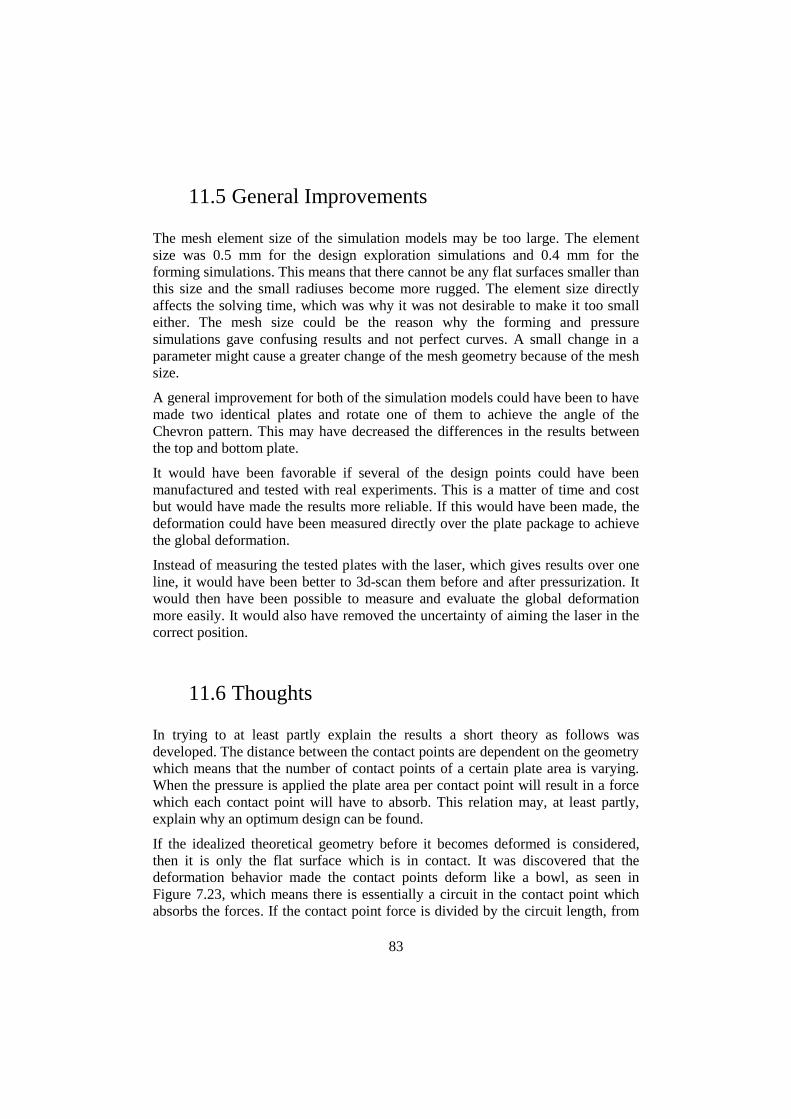
83
11.5 General Improvements
The mesh element size of the simulation models may be too large. The element
size was 0.5 mm for the design exploration simulations and 0.4 mm for the
forming simulations. This means that there cannot be any flat surfaces smaller than
this size and the small radiuses become more rugged. The element size directly
affects the solving time, which was why it was not desirable to make it too small
either. The mesh size could be the reason why the forming and pressure
simulations gave confusing results and not perfect curves. A small change in a
parameter might cause a greater change of the mesh geometry because of the mesh
size.
A general improvement for both of the simulation models could have been to have
made two identical plates and rotate one of them to achieve the angle of the
Chevron pattern. This may have decreased the differences in the results between
the top and bottom plate.
It would have been favorable if several of the design points could have been
manufactured and tested with real experiments. This is a matter of time and cost
but would have made the results more reliable. If this would have been made, the
deformation could have been measured directly over the plate package to achieve
the global deformation.
Instead of measuring the tested plates with the laser, which gives results over one
line, it would have been better to 3d-scan them before and after pressurization. It
would then have been possible to measure and evaluate the global deformation
more easily. It would also have removed the uncertainty of aiming the laser in the
correct position.
11.6 Thoughts
In trying to at least partly explain the results a short theory as follows was
developed. The distance between the contact points are dependent on the geometry
which means that the number of contact points of a certain plate area is varying.
When the pressure is applied the plate area per contact point will result in a force
which each contact point will have to absorb. This relation may, at least partly,
explain why an optimum design can be found.
If the idealized theoretical geometry before it becomes deformed is considered,
then it is only the flat surface which is in contact. It was discovered that the
deformation behavior made the contact points deform like a bowl, as seen in
Figure 7.23, which means there is essentially a circuit in the contact point which
absorbs the forces. If the contact point force is divided by the circuit length, from
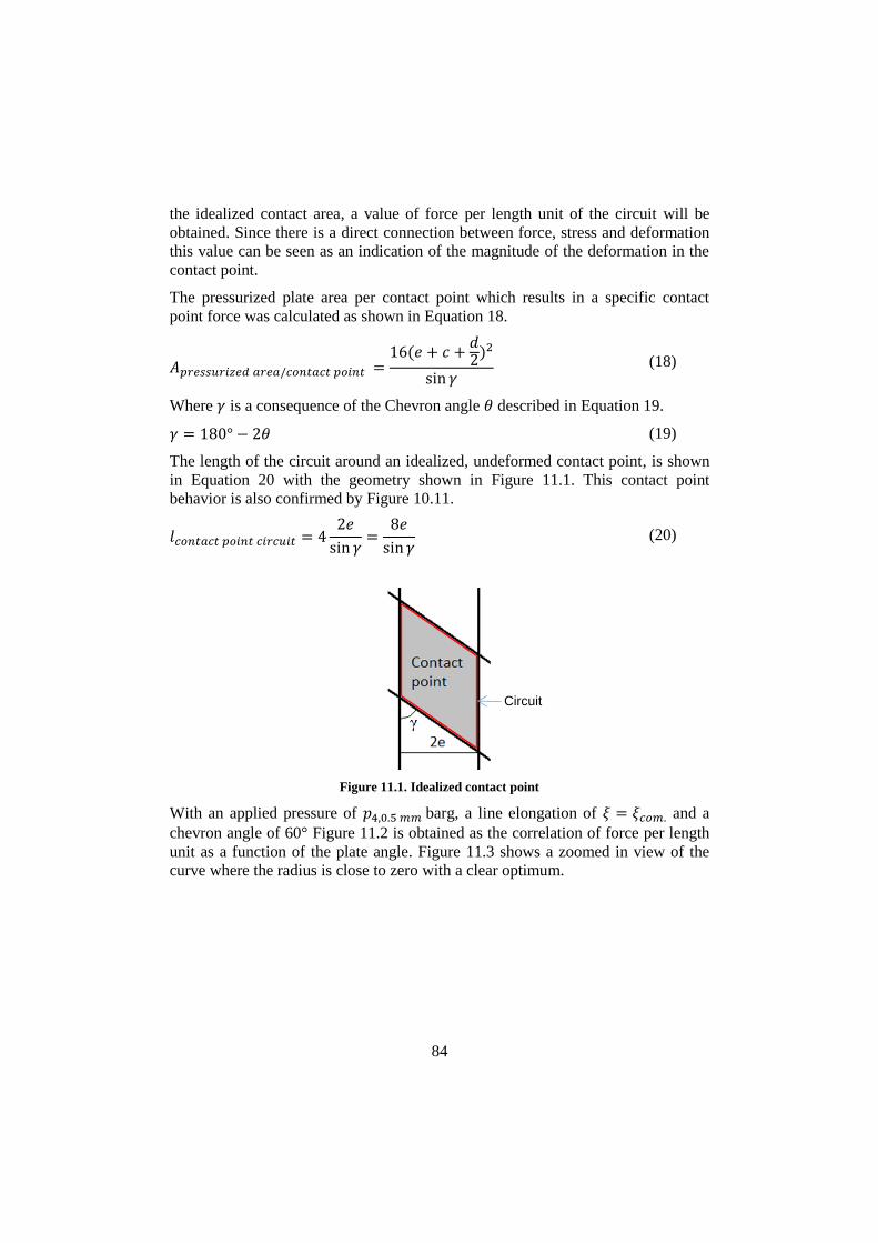
84
the idealized contact area, a value of force per length unit of the circuit will be
obtained. Since there is a direct connection between force, stress and deformation
this value can be seen as an indication of the magnitude of the deformation in the
contact point.
The pressurized plate area per contact point which results in a specific contact
point force was calculated as shown in Equation 18.
𝐴𝑝𝑟𝑒𝑠𝑠𝑢𝑟𝑖𝑧𝑒𝑑 𝑎𝑟𝑒𝑎/𝑐𝑜𝑛𝑡𝑎𝑐𝑡 𝑝𝑜𝑖𝑛𝑡 =16(𝑒 + 𝑐 +
𝑑2
)2
sin 𝛾 (18)
Where 𝛾 is a consequence of the Chevron angle 𝜃 described in Equation 19.
𝛾 = 180° − 2𝜃 (19)
The length of the circuit around an idealized, undeformed contact point, is shown
in Equation 20 with the geometry shown in Figure 11.1. This contact point
behavior is also confirmed by Figure 10.11.
𝑙𝑐𝑜𝑛𝑡𝑎𝑐𝑡 𝑝𝑜𝑖𝑛𝑡 𝑐𝑖𝑟𝑐𝑢𝑖𝑡 = 42𝑒
sin 𝛾=
8𝑒
sin 𝛾 (20)
Figure 11.1. Idealized contact point
With an applied pressure of 𝑝4,0.5 𝑚𝑚 barg, a line elongation of 𝜉 = 𝜉𝑐𝑜𝑚. and a
chevron angle of 60° Figure 11.2 is obtained as the correlation of force per length
unit as a function of the plate angle. Figure 11.3 shows a zoomed in view of the
curve where the radius is close to zero with a clear optimum.
Circuit
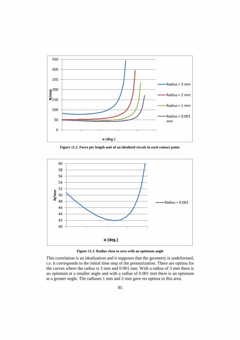
85
Figure 11.2. Force per length unit of an idealized circuit in each contact point.
Figure 11.3. Radius close to zero with an optimum angle
This correlation is an idealization and it supposes that the geometry is undeformed,
i.e. it corresponds to the initial time step of the pressurization. There are optima for
the curves where the radius is 3 mm and 0.001 mm. With a radius of 3 mm there is
an optimum at a smaller angle and with a radius of 0.001 mm there is an optimum
at a greater angle. The radiuses 1 mm and 2 mm gave no optima in this area.
0
50
100
150
200
250
300
350
10 20 30 40 50 60
N/m
m
α (deg.)
Radius = 3 mm
Radius = 2 mm
Radius = 1 mm
Radius = 0.001mm
40
42
44
46
48
50
52
54
56
58
60
10 20 30 40 50
N/m
m
α (deg.)
Radius = 0.001

86
The reason for the curves turning straight upwards with an increasing angle is that
the flat contact surface and the circuit become close to zero. A probable
explanation to why the simulation results do not increases this fast is that in reality
there is an immediate deformation which increases the contact area and circuit
length. If the contact area from the beginning is close to zero a small absolute
increase will result in a great relative increase. This means that if a compensation
is made for what happens when the deformation has started concerning the points
with a greater angle the stress will decrease faster than for the points with a minor
angle. If that argument is correct, it could explain why there also are optima for
radiuses of 𝑟2 mm and 𝑟3 + 0.25 mm and why the real optima are located further
to the right (i.e. greater angles) than what can be seen in this theoretical model.
87
11.7 Conclusions
Regarding the geometry, the conclusion is that the radius should be as small as
possible. It is not as easy to give an exact answer about the plate angle. Generally
an angle around 𝛼2, seen in Figure 10.16, can be an appropriate target. Angles
between 𝛼1 and 𝛼2 can be the optimum. The other parameters must also be
evaluated in the choice of design. A mechanically optimized design could be
similar to what is shown in Figure 7.2 where the flat surface is relatively large. In
a thermal perspective this might not be ideal since the area of the contact points
are not directly heat transferring.
Regarding the simulation models the conclusions are that the existing forming and
pressure simulations used by Alfa Laval work well and correspond acceptably to
reality. The simulations made for the design exploration were relatively far from
reality. Nonetheless, it was a useful tool for examining the behavior of the
geometry.
It seems likely that the local deformation stands for the major part of the total
deformations, but it was only confirmed by the first rough simulation model. It
was seen that the global deformations are difficult to measure on a single plate.
11.8 Recommendations for Future Work
One recommendation would be to carry out laboratory experiments in order to
investigate the difference between local and global. If the total deformation on a
whole plate package is measured and divided by the number of plates, the global
deformation for one plate would be obtained. The local deformation for a single
plate can then be measured and a comparison can be made.
It would have been interesting to investigate the behavior of titanium plates to see
if the material properties have any major impact on the deformation behavior.
Investigating and confirming how the conclusions correspond to different plate
depths and plate thicknesses would have been valuable.
Doing laboratory experiments of different plate geometries in the same way as the
simulations were done would give a greater credibility to the results of the thesis.

89
References
[1] Alfa Laval. (2015). Retrieved March 1, 2016, from: http://www.alfalaval.com/.
[2] ASME (American Society of Mechanical Engineers). (2016). Retrieved March
2, 2016, from: https://www.asme.org/shop/certification-and-
accreditation/boiler-and-pressure-vessel-certification.
[3] European Comission. (2016). Retrieved March 2, 2016, from:
http://ec.europa.eu/growth/sectors/pressure-gas/pressure-
equipment/directive/index_en.htm.
[4] Ottosen N, Petersson H. (1992) Introduction to the Finite Element Method.
Lund, Sweden: Prentice Hall.
[5] LSTC Inc; Dynamore. Ls-dyna Support. (2016). Retrieved March 11, 2016,
from: http://www.dynasupport.com/faq/general/what-are-the-differences-
between-implicit-and-explicit.
[6] Barlat F, Lian J. (1989) Plastic behavior and stretchability of sheet metals. Part
I: A yield function for orthotropic sheets under plane stress conditions.
International Journal of Plasticity.


Appendix A Time Schedule
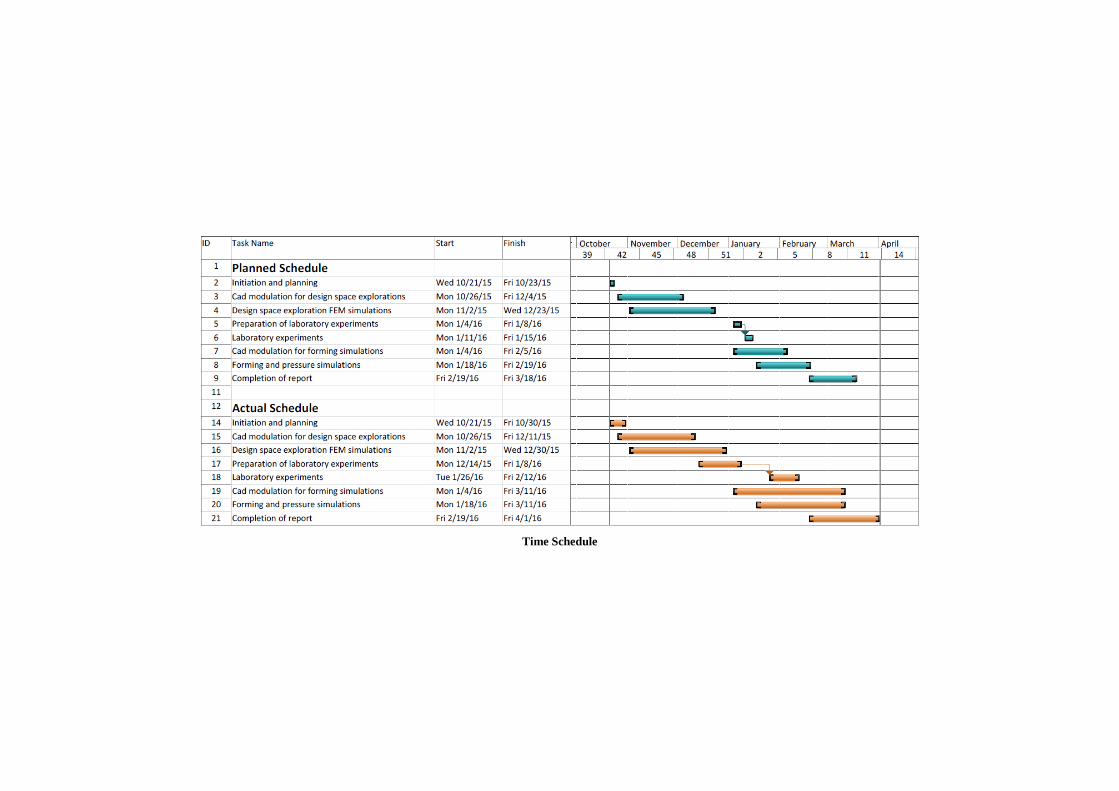
Time Schedule
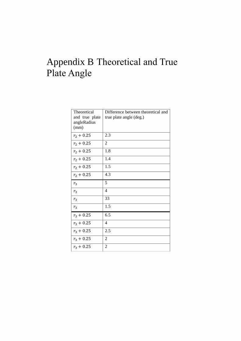
Appendix B Theoretical and True
Plate Angle
Theoretical
and true plate
angleRadius
(mm)
Difference between theoretical and
true plate angle (deg.)
𝑟2 + 0.25 2.3
𝑟2 + 0.25 2
𝑟2 + 0.25 1.8
𝑟2 + 0.25 1.4
𝑟2 + 0.25 1.5
𝑟2 + 0.25 4.3
𝑟3 5
𝑟3 4
𝑟3 33
𝑟3 1.5
𝑟3 + 0.25 6.5
𝑟3 + 0.25 4
𝑟3 + 0.25 2.5
𝑟3 + 0.25 2
𝑟3 + 0.25 2