Embed Size (px)
Citation preview
Deformation-Invariant Sparse Coding
by
George H. Chen
B.S. with dual majors in Electrical Engineering and Computer Sciences,Engineering Mathematics and Statistics, UC Berkeley, May 2010
Submitted to the Department of Electrical Engineering and Computer Sciencein partial fulfillment of the requirements for the degree of
Master of Sciencein Electrical Engineering and Computer Science
at the Massachusetts Institute of Technology
June 2012
c© 2012 Massachusetts Institute of TechnologyAll Rights Reserved.
Signature of Author:
George H. ChenDepartment of Electrical Engineering and Computer Science
May 23, 2012
Certified by:
Polina GollandAssociate Professor of Electrical Engineering and Computer Science
Thesis Supervisor
Accepted by:
Leslie A. KolodziejskiProfessor of Electrical Engineering and Computer Science
Chair, Committee for Graduate Students

2
Deformation-Invariant Sparse Codingby George H. Chen
Submitted to the Department of Electrical Engineering and Computer Sciencein partial fulfillment of the requirements for the degree of
Master of Science
AbstractSparse coding represents input signals each as a sparse linear combination of a set ofbasis or dictionary elements where sparsity encourages representing each input signalwith a few of the most indicative dictionary elements. In this thesis, we extend sparsecoding to allow dictionary elements to undergo deformations, resulting in a generalprobabilistic model and accompanying inference algorithm for estimating sparse linearcombination weights, dictionary elements, and deformations.
We apply our proposed method on functional magnetic resonance imaging (fMRI)data, where the locations of functional regions in the brain evoked by a specific cognitivetask may vary across individuals relative to anatomy. For a language fMRI study,our method identifies activation regions that agree with known literature on languageprocessing. Furthermore, the deformations learned by our inference algorithm producemore robust group-level effects than anatomical alignment alone.
Thesis Supervisor: Polina GollandTitle: Associate Professor of Electrical Engineering and Computer Science
3

4
Acknowledgements
The past two years have been a tumultuous success, thanks to an incredible cast of
people who’ve helped me along the way. At the forefront of this cast is Polina Golland,
who has been a phenomenal advisor. Polina has provided me insight into a slew of
problems, and I’ve lost count of how many times I’ve crashed into a road block, she’d
suggest a way to visualize data for debugging, and—voila—road block demolished! At
the same time, Polina has been tremendously chill, letting me toil at my own pace
while I sporadically derail myself with side interests divergent from the Golland group.
Thanks Polina, and thanks for ensuring that I don’t derail myself too much!
This thesis would not have seen the light of day without the assistance of my collab-
orators Ev Fedorenko and Nancy Kanwisher. As I have no background in neuroscience,
Ev and Nancy were instrumental in explaining some of the basics and offered invaluable
comments, feedback, and data on the neuroscience application that drives this thesis.
It really was the neuroscience application that led to the main model proposed in this
thesis rather than the other way around.
Meanwhile, landing in Polina’s group was a culture shock in itself as my background
was not in medical imaging. Luckily, members of the group have been more than ac-
commodating. Without the patience of former group members Danial Lashkari, Gabriel
Tobon, and Michal Depa in answering my barrage of questions on functional magnetic
resonance imaging and image registration during my first year, my transition into work-
ing in medical imaging would have taken substantially longer with at least a tenfold
increase in headaches, futility, and despair. I would also like to thank the rest of the
group members for far too many delightful conversations and for putting up with my
recurring bouts of frustration and fist shaking. Numerous thanks also go out to visiting
group members Rene Donner, who hosted me in Austria, and Prof. Georg Langs, whose
bicycle that I’m still borrowing has immensely improved my quality of life.
5

6
Many students outside of Polina’s group have also had a remarkable impact on
my education and crusade against grad-student-depressionitis. Eric Trieu has been a
repository of great conversations, puns, and medical advice. James Saunderson has
been my encyclopedia for math and optimization. As for machine learning, I have
yet to meet any grad student who has amassed more machine learning knowledge and
big-picture understanding than Roger Grosse, who persistently is rewarding to bounce
ideas off of. I also want to thank the rest of the computer vision and Stochastic Systems
Group students for all the productive discussions as well as new ways to procrastinate.
To solidify my understanding of probabilistic graphical models, I had the fortune of
being a teaching assistant for Devavrat Shah and Greg Wornell, who were an absolute
riot to work with. Too often, their perspectives on problems led me to all sorts of new
intuitions and epiphanies. Many thanks also go to my co-TA’s Roger Grosse (again)
and George Tucker, who contributed to my project of making Khan Academy style
videos for the students. I still can’t believe we threw together all those videos and
churned out the first ever complete set of typeset lecture notes for 6.438!
Outside of academics, I’ve had the pleasure and extraordinary experience of being
an officer in the Sidney Pacific Graduate Residence. I would like to thank all the other
officers who helped me serve the full palate of artsy, marginally educational, and down-
right outrageous competitive dorm events throughout the 2011-2012 academic year,
and all the residents who participated, not realizing that they were actually helpless
test subjects. My only hope is that I didn’t accidentally deplete all the dorm funds.
I would especially like to thank Brian Spatocco for being an exceptional mentor and
collaborator, helping me become a far better event organizer than I imagined myself
being at the start of grad school.
I end by thanking my brother and my parents for their support over the years.
Contents
Abstract 3
Acknowledgements 4
List of Figures 9
1 Introduction 11
2 Background 15
2.1 Images, Deformations, Qualitative Spaces, and Masks . . . . . . . . . . 15
2.2 Sparse Coding . . . . . . . . . . . . . . . . . . . . . . . . . . . . . . . . 17
2.3 Estimating a Deformation that Aligns Two Images . . . . . . . . . . . . 20
2.3.1 Pairwise Image Registration as an Optimization Problem . . . . 20
2.3.2 Diffeomorphic Demons Registration . . . . . . . . . . . . . . . . 21
2.4 Estimating Deformations that Align a Group of Images . . . . . . . . . 24
2.4.1 Parallel Groupwise Image Registration . . . . . . . . . . . . . . . 26
2.4.2 Serial Groupwise Image Registration . . . . . . . . . . . . . . . . 27
2.5 Finding Group-level Functional Brain Activations in fMRI . . . . . . . . 27
3 Probabilistic Deformation-Invariant Sparse Coding 31
3.1 Formulation . . . . . . . . . . . . . . . . . . . . . . . . . . . . . . . . . . 31
3.1.1 Model Parameters . . . . . . . . . . . . . . . . . . . . . . . . . . 33
3.1.2 Relation to Sparse Coding . . . . . . . . . . . . . . . . . . . . . . 36
3.2 Inference . . . . . . . . . . . . . . . . . . . . . . . . . . . . . . . . . . . . 36
3.2.1 Initialization . . . . . . . . . . . . . . . . . . . . . . . . . . . . . 41
3.2.2 Intensity-equalization Interpretation . . . . . . . . . . . . . . . . 41
3.3 Extensions . . . . . . . . . . . . . . . . . . . . . . . . . . . . . . . . . . . 42
7
8 CONTENTS
4 Modeling Spatial Variability of Functional Patterns in the Brain 47
4.1 Instantiation to fMRI Analysis . . . . . . . . . . . . . . . . . . . . . . . 47
4.2 Hyperparameter Selection . . . . . . . . . . . . . . . . . . . . . . . . . . 51
4.2.1 Cross-validation Based on Limited Ground Truth . . . . . . . . . 51
4.2.2 Heuristics in the Absence of Ground Truth . . . . . . . . . . . . 53
4.3 Synthetic Data . . . . . . . . . . . . . . . . . . . . . . . . . . . . . . . . 56
4.3.1 Data Generation . . . . . . . . . . . . . . . . . . . . . . . . . . . 56
4.3.2 Evaluation . . . . . . . . . . . . . . . . . . . . . . . . . . . . . . 57
4.3.3 Results . . . . . . . . . . . . . . . . . . . . . . . . . . . . . . . . 58
4.4 Language fMRI Study . . . . . . . . . . . . . . . . . . . . . . . . . . . . 62
4.4.1 Data . . . . . . . . . . . . . . . . . . . . . . . . . . . . . . . . . . 63
4.4.2 Evaluation . . . . . . . . . . . . . . . . . . . . . . . . . . . . . . 63
4.4.3 Results . . . . . . . . . . . . . . . . . . . . . . . . . . . . . . . . 64
5 Discussion and Conclusions 69
A Deriving the Inference Algorithm 71
A.1 E-step . . . . . . . . . . . . . . . . . . . . . . . . . . . . . . . . . . . . . 74
A.2 M-step: Updating Deformations Φ . . . . . . . . . . . . . . . . . . . . . 76
A.3 M-step: Updating Parameters λ and σ2 . . . . . . . . . . . . . . . . . . 77
A.4 M-step: Updating Dictionary D . . . . . . . . . . . . . . . . . . . . . . 78
B Deriving the Specialized Inference Algorithm for Chapter 4 83
Bibliography 87
List of Figures
1.1 Toy example observed signals. . . . . . . . . . . . . . . . . . . . . . . . . 11
1.2 Toy example average signal. . . . . . . . . . . . . . . . . . . . . . . . . . 12
1.3 Toy example observed signals that have undergone shifts. . . . . . . . . 12
1.4 Toy example average of the shifted signals. . . . . . . . . . . . . . . . . 13
2.1 A probabilistic graphical model for sparse coding. . . . . . . . . . . . . . 19
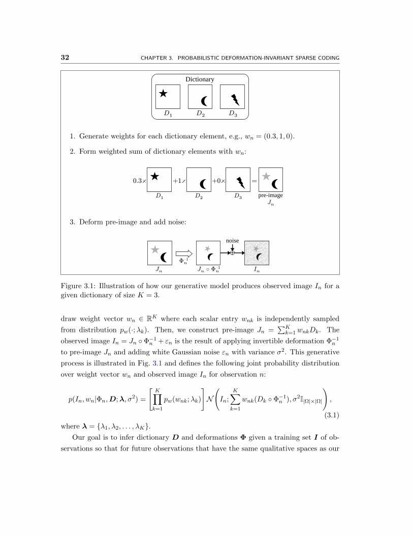
3.1 Illustration of how our generative model produces observed image In for
a given dictionary of size K = 3. . . . . . . . . . . . . . . . . . . . . . . 32
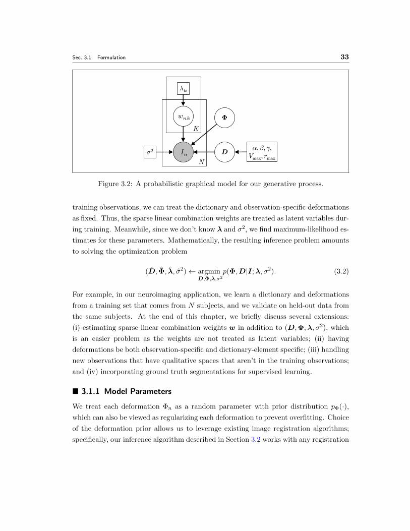
3.2 A probabilistic graphical model for our generative process. . . . . . . . . 33
4.1 The synthetic data’s (a) true dictionary, and estimated dictionaries us-
ing (b) the watershed baseline, (c) the sparse coding baseline, and (d)
deformation-invariant sparse coding. . . . . . . . . . . . . . . . . . . . . 60
4.2 Synthetic data examples of pre-images and their corresponding observed
images. All images are shown with the same intensity scale. . . . . . . . 61
4.3 Synthetic data average of test images (a) without deformations, and
(b) aligned with deformations estimated from training data using deformation-
invariant sparse coding. Both images are shown with the same intensity
scale and zoomed in. . . . . . . . . . . . . . . . . . . . . . . . . . . . . . 61
4.4 Scatter plot used to evaluate hyperparameter selection heuristics for syn-
thetic data. Each hyperparameter setting (α, β, γ) is depicted as a single
point, where α, β, γ ∈ 0, 102, 104, 106. The top 5 hyperparameter set-
tings (some overlap in the plot) according to our group average error on
test data are shown in red; all other hyperparameter settings are shown
in blue. . . . . . . . . . . . . . . . . . . . . . . . . . . . . . . . . . . . . 62
9
10 LIST OF FIGURES
4.5 Scatter plot used to evaluate hyperparameter selection heuristics for lan-
guage fMRI data. Each hyperparameter setting (α, β, γ) is depicted
as a single point, where α, β, γ ∈ 0, 102, 104, 106, 108. Hyperparam-
eter settings in red and green have comparable dictionary consistency,
Hintensity-improvement-difference < 0.1, and Hintensity-improvement > 0.4. Hy-
perparameter settings in green further achieve Hintensity-improvement > 0.6. 65
4.6 Estimated dictionary. (a) Four slices of a map showing the spatial sup-
port of the extracted dictionary elements. Different colors correspond to
distinct dictionary elements where there is some overlap between dictio-
nary elements. From left to right: left frontal lobe and temporal regions,
medial prefrontal cortex and posterior cingulate/precuneus, right cere-
bellum, and right temporal lobe. Dictionary element indices correspond
to those in Fig. 4.7. (b) A single slice from three different estimated
dictionary elements where relative intensity varies from high (red) to
low (blue). From left to right: left posterior temporal lobe, left anterior
temporal lobe, left inferior frontal gyrus. . . . . . . . . . . . . . . . . . . 66
4.7 Box plots of top 25% weighted random effects analysis significance val-
ues within dictionary element supports. For each dictionary element,
“A” refers to anatomical alignment, and “F” refers to alignment via de-
formations learned by our model. . . . . . . . . . . . . . . . . . . . . . 66
4.8 Box plots of top 50% weighted random effects analysis significance val-
ues within dictionary element supports. For each dictionary element,
“A” refers to anatomical alignment, and “F” refers to alignment via de-
formations learned by our model. . . . . . . . . . . . . . . . . . . . . . 67
4.9 Box plots of top 1% weighted random effects analysis significance values
within dictionary element supports. For each dictionary element, “A”
refers to anatomical alignment, and “F” refers to alignment via deforma-
tions learned by our model. . . . . . . . . . . . . . . . . . . . . . . . . . 67
Chapter 1
Introduction
FINDING succinct representations for signals such as images and audio enable us to
glean high-level features in data. For example, an image may be represented as a
sum of a small number of edges or patches, and the presence of certain edges and patches
may be used as features for object recognition. As another example, given a household’s
electricity usage over time, representing this signal as a sum of contributions from
different electrical devices could allow us to pinpoint the culprits for a high electricity
bill. These scenarios exemplify sparse coding, which refers to representing an input
signal as a sparse linear combination of basis or dictionary elements, where sparsity
selects the most indicative dictionary elements that explain our data. The focus of this
thesis is on estimating these dictionary elements and, in particular, extending sparse
coding to allow dictionary elements to undergo potentially nonlinear deformations.
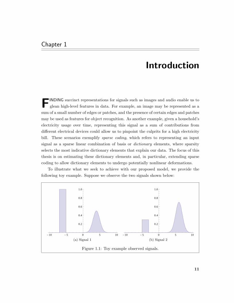
To illustrate what we seek to achieve with our proposed model, we provide the
following toy example. Suppose we observe the two signals shown below:
- 10 - 5 0 5 10
0.2
0.4
0.6
0.8
1.0
(a) Signal 1
- 10 - 5 0 5 10
0.2
0.4
0.6
0.8
1.0
(b) Signal 2
Figure 1.1: Toy example observed signals.
11
12 CHAPTER 1. INTRODUCTION
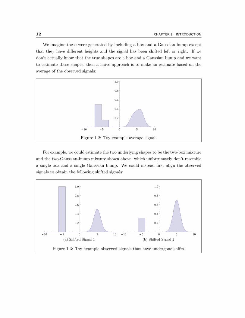
We imagine these were generated by including a box and a Gaussian bump except
that they have different heights and the signal has been shifted left or right. If we
don’t actually know that the true shapes are a box and a Gaussian bump and we want
to estimate these shapes, then a naive approach is to make an estimate based on the
average of the observed signals:
- 10 - 5 0 5 10
0.2
0.4
0.6
0.8
1.0
Figure 1.2: Toy example average signal.
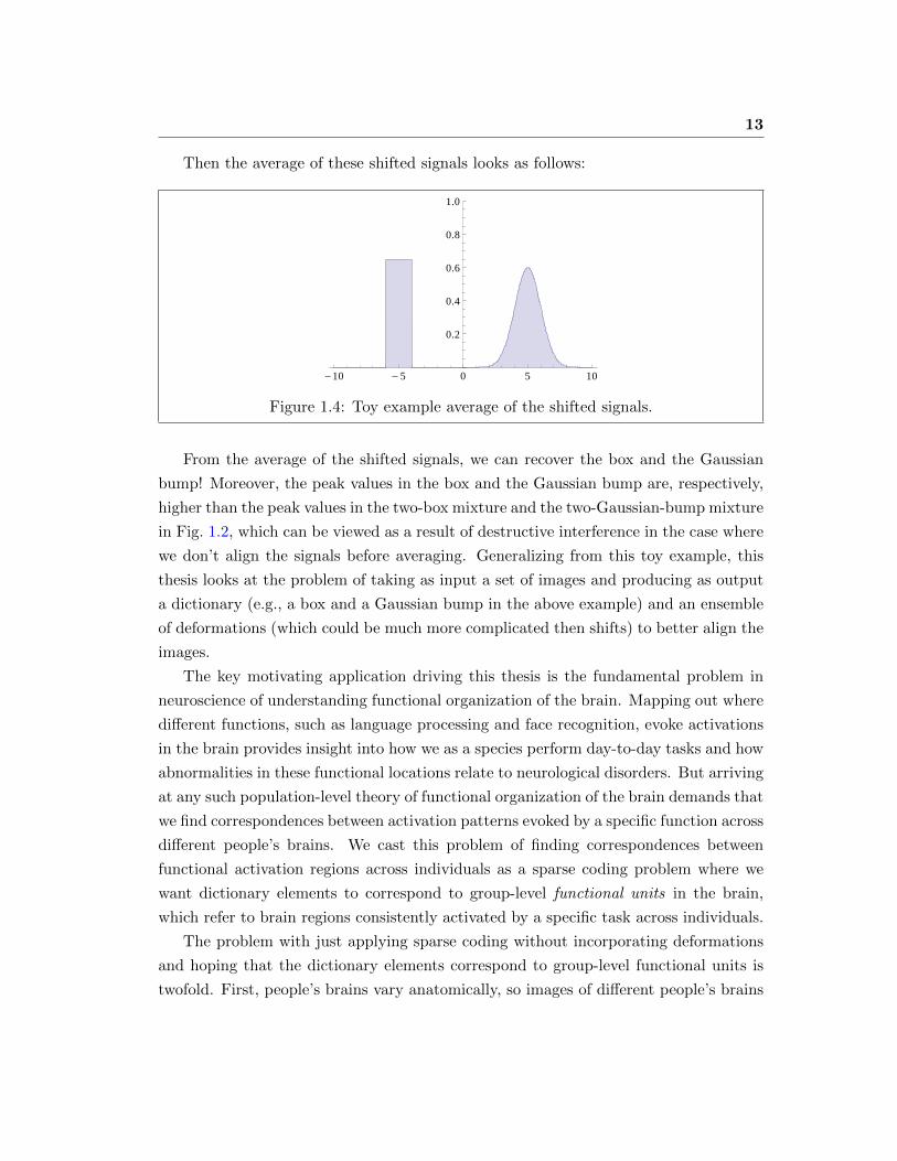
For example, we could estimate the two underlying shapes to be the two-box mixture
and the two-Gaussian-bump mixture shown above, which unfortunately don’t resemble
a single box and a single Gaussian bump. We could instead first align the observed
signals to obtain the following shifted signals:
- 10 - 5 0 5 10
0.2
0.4
0.6
0.8
1.0
(a) Shifted Signal 1
- 10 - 5 0 5 10
0.2
0.4
0.6
0.8
1.0
(b) Shifted Signal 2
Figure 1.3: Toy example observed signals that have undergone shifts.
13
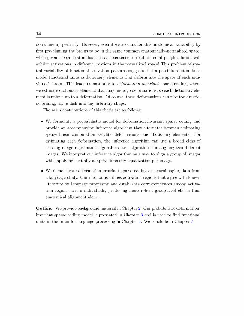
Then the average of these shifted signals looks as follows:
- 10 - 5 0 5 10
0.2
0.4
0.6
0.8
1.0
Figure 1.4: Toy example average of the shifted signals.
From the average of the shifted signals, we can recover the box and the Gaussian
bump! Moreover, the peak values in the box and the Gaussian bump are, respectively,
higher than the peak values in the two-box mixture and the two-Gaussian-bump mixture
in Fig. 1.2, which can be viewed as a result of destructive interference in the case where
we don’t align the signals before averaging. Generalizing from this toy example, this
thesis looks at the problem of taking as input a set of images and producing as output
a dictionary (e.g., a box and a Gaussian bump in the above example) and an ensemble
of deformations (which could be much more complicated then shifts) to better align the
images.
The key motivating application driving this thesis is the fundamental problem in
neuroscience of understanding functional organization of the brain. Mapping out where
different functions, such as language processing and face recognition, evoke activations
in the brain provides insight into how we as a species perform day-to-day tasks and how
abnormalities in these functional locations relate to neurological disorders. But arriving
at any such population-level theory of functional organization of the brain demands that
we find correspondences between activation patterns evoked by a specific function across
different people’s brains. We cast this problem of finding correspondences between
functional activation regions across individuals as a sparse coding problem where we
want dictionary elements to correspond to group-level functional units in the brain,
which refer to brain regions consistently activated by a specific task across individuals.
The problem with just applying sparse coding without incorporating deformations
and hoping that the dictionary elements correspond to group-level functional units is
twofold. First, people’s brains vary anatomically, so images of different people’s brains
14 CHAPTER 1. INTRODUCTION
don’t line up perfectly. However, even if we account for this anatomical variability by
first pre-aligning the brains to be in the same common anatomically-normalized space,
when given the same stimulus such as a sentence to read, different people’s brains will
exhibit activations in different locations in the normalized space! This problem of spa-
tial variability of functional activation patterns suggests that a possible solution is to
model functional units as dictionary elements that deform into the space of each indi-
vidual’s brain. This leads us naturally to deformation-invariant sparse coding, where
we estimate dictionary elements that may undergo deformations, so each dictionary ele-
ment is unique up to a deformation. Of course, these deformations can’t be too drastic,
deforming, say, a disk into any arbitrary shape.
The main contributions of this thesis are as follows:
• We formulate a probabilistic model for deformation-invariant sparse coding and
provide an accompanying inference algorithm that alternates between estimating
sparse linear combination weights, deformations, and dictionary elements. For
estimating each deformation, the inference algorithm can use a broad class of
existing image registration algorithms, i.e., algorithms for aligning two different
images. We interpret our inference algorithm as a way to align a group of images
while applying spatially-adaptive intensity equalization per image.
• We demonstrate deformation-invariant sparse coding on neuroimaging data from
a language study. Our method identifies activation regions that agree with known
literature on language processing and establishes correspondences among activa-
tion regions across individuals, producing more robust group-level effects than
anatomical alignment alone.
Outline. We provide background material in Chapter 2. Our probabilistic deformation-
invariant sparse coding model is presented in Chapter 3 and is used to find functional
units in the brain for language processing in Chapter 4. We conclude in Chapter 5.

Chapter 2
Background
We begin this chapter by describing how images and deformations are represented
throughout this thesis including notation used. We then provide background material
on sparse coding, estimating deformations for aligning images, and finding group-level
brain activations evoked by functional stimuli in functional magnetic resonance imag-
ing (fMRI).
2.1 Images, Deformations, Qualitative Spaces, and Masks
To represent images and deformations, we first define the space in which they exist.
Consider a finite, discrete set of points Ω ⊂ Rd that consists of coordinates in d-
dimensional space that are referred to as pixels for 2D images (d = 2) and volumetric
pixels or voxels for 3D images (d = 3). For simplicity, we refer to elements of Ω as
voxels when working with signals that are not 3D images.
We represent an image in two different ways: as a vector in R|Ω| and as a function
that maps Ω to R. Specifically, for an image I, we write I ∈ R|Ω| (vector representation)
and use indexing notation I(x) ∈ R to mean the intensity value of image I at voxel x ∈ Ω
(functional representation). These two representations are equivalent: by associating
each voxel x ∈ Ω with a unique index in 1, 2, . . . , |Ω|, value I(x) becomes just the
value of vector I ∈ R|Ω| at the index associated with voxel x.
But what if we want to know the value of an image at a voxel that’s not in Ω?
To handle this, we extend notation by allowing indexing into an image I ∈ R|Ω| by a
voxel that may not be in Ω. Specifically, we allow indexing into a voxel in Ωc, which
is a continuous extension Ωc of Ω, where formally Ωc is a simply-connected open set
that contains Ω. This means that Ωc is a region comprising of a single connected
component, does not have any holes in it, and contains the convex hull of Ω. Then I(y)
for y ∈ Ωc \ Ω refers to an interpolated value of image I at voxel y /∈ Ω; e.g., nearest-
15

16 CHAPTER 2. BACKGROUND
neighbor interpolation would simply involve finding x ∈ Ω closest in Euclidean distance
to voxel y and outputting I(y)← I(x).
Next, we discuss deformations, which use interpolation. We define a deformation Φ
as a mapping from Ωc to Ωc. Note that if Φ only mapped from Ω to Ω, then Φ
would just be a permutation, which is insufficient for our purposes. We work with
deformations that are diffeomorphisms, which means that they are invertible and both
the deformations and their inverses have continuous derivatives of all orders. We let
|JΦ(x)| denote the Jacobian determinant of Φ evaluated at voxel x. Crucially, |JΦ(x)|can be interpreted as the volume change ratio for voxel x due to deformation Φ, i.e.,
|JΦ(x)| partial voxels from the input space of Φ warps to voxel x in the output space
of Φ. To see this, consider a compactly supported, continuous function f : Ωc → R.
From calculus, we have ∫Ωc
f(Φ−1(x))dx =
∫Ωc
f(x)|JΦ(x)|dx. (2.1)
Observe that voxel x has weight |JΦ(x)| in image f while it has weight 1 in image
f Φ−1. Thus, due to applying Φ to f Φ−1 to obtain f , the “volume” at voxel x
changes from 1 to |JΦ(x)|. This intuition of volume change will be apparent when we
discuss averaging deformed images later in this chapter. Also, as eq. (2.1) suggests,
for Φ to be invertible, we must have |JΦ(x)| > 0 for all x ∈ Ωc.
We can interpret deformation Φ as a change of coordinates that may potentially be
nonlinear; Φ deforms an input space to an output space and while both input and output
spaces are Ωc, they may have very qualitative meanings! For example, for Ωc = R+ (the
positive real line) and Φ(x) = log(x + 1), if the input space is in units of millimeters,
then the output space, while also being R+, is in units of log millimeters. Thus, each
image is associated with a qualitative space (e.g., millimeter space, log-millimeter space,
the anatomical space of Alice’s brain, the anatomical space of Bob’s brain).
With an image I and deformation Φ, we can define deformed image I Φ ∈ R|Ω|
using our functional representation for images:
(I Φ)(x) = I(Φ(x)) for x ∈ Ω,
where Φ(x) could be in Ωc \ Ω, requiring interpolation. Importantly, image I Φ has
the interpretation of image I being deformed by Φ such that I Φ now has coordinates
defined by the input space of Φ.

Sec. 2.2. Sparse Coding 17
Henceforth, when dealing with images, we often omit writing out the voxel space Ω
and liberally switch between using vector and functional representations for images. We
typically use variable x to denote a voxel. In this work, we consider diffeomorphisms
and note that by setting Ωc = Rd, then translations, rotations, and invertible affine
transformations are all examples of diffeomorphisms mapping Ωc to Ωc.
2.2 Sparse Coding
As mentioned previously, sparse coding refers to representing an input signal as a sparse
linear combination of dictionary elements. For example, sparse coding applied to natural
images can learn dictionary elements resembling spatial receptive fields of neurons in
the visual cortex [27, 28]. Applied to images, video, and audio, sparse coding can
learn dictionary elements that represent localized bases [12, 23, 25, 27, 28, 40]. In this
section, we review sparse coding, its associated optimization problem, its probabilistic
interpretation, and its relation to factor analysis.
In sparse coding, we model observations I1, I2 . . . , IN ∈ RP to be generated from
dictionary elements D1, D2, . . . , DK ∈ RP as follows:
In =
K∑k=1
wnkDk + εn for n = 1, 2, . . . , N, (2.2)
where weights wn ∈ RK are sparse (i.e., mostly zero), and noise εn ∈ Rd is associated
with observation n. For notational convenience, we write eq. (2.2) in matrix form:
I = Dw + ε, (2.3)
where we stack column vectors to form matrices I = [I1|I2| · · · |IN ] ∈ RP×N , D =
[D1|D2| · · · |DK ] ∈ RP×K , w = [w1|w2| · · · |wN ] ∈ RK×N , and ε = [ε1|ε2| · · · |εN ] ∈RP×N . We aim to find dictionary D and sparse weights w that minimize data-fitting
error ‖I −Dw‖2F =∑N
n=1 ‖In −Dwn‖22, where ‖ · ‖F and ‖ · ‖2 refer to the Frobenius
and Euclidean norms, respectively.
However, as written, finding dictionary D and sparse weights w is an ill-posed
problem because scaling weight wnk by some constant c > 0 for all n while scaling
dictionary element Dk by 1/c results in the same observation I. Thus, we require
a constraint on either the weights or the dictionary elements. Often a constraint is
placed on the latter by requiring ‖Dk‖2 ≤ 1 for each k. A less worrisome issue is that
18 CHAPTER 2. BACKGROUND
permuting the dictionary elements and their associated weights also yields the same
observed signal; this is addressed by just recognizing that the ordering of estimated
dictionary elements is not unique.
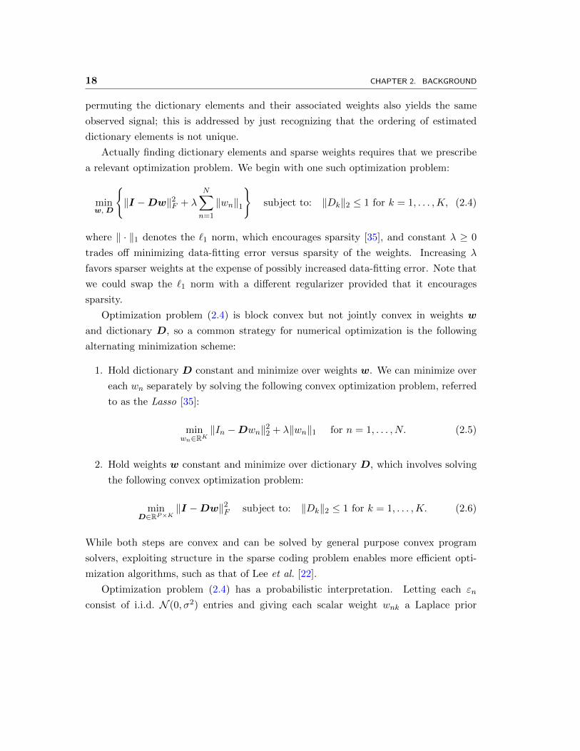
Actually finding dictionary elements and sparse weights requires that we prescribe
a relevant optimization problem. We begin with one such optimization problem:
minw,D
‖I −Dw‖2F + λ
N∑n=1
‖wn‖1
subject to: ‖Dk‖2 ≤ 1 for k = 1, . . . ,K, (2.4)
where ‖ · ‖1 denotes the `1 norm, which encourages sparsity [35], and constant λ ≥ 0
trades off minimizing data-fitting error versus sparsity of the weights. Increasing λ
favors sparser weights at the expense of possibly increased data-fitting error. Note that
we could swap the `1 norm with a different regularizer provided that it encourages
sparsity.
Optimization problem (2.4) is block convex but not jointly convex in weights w
and dictionary D, so a common strategy for numerical optimization is the following
alternating minimization scheme:
1. Hold dictionary D constant and minimize over weights w. We can minimize over
each wn separately by solving the following convex optimization problem, referred
to as the Lasso [35]:
minwn∈RK
‖In −Dwn‖22 + λ‖wn‖1 for n = 1, . . . , N. (2.5)
2. Hold weights w constant and minimize over dictionary D, which involves solving
the following convex optimization problem:
minD∈RP×K
‖I −Dw‖2F subject to: ‖Dk‖2 ≤ 1 for k = 1, . . . ,K. (2.6)
While both steps are convex and can be solved by general purpose convex program
solvers, exploiting structure in the sparse coding problem enables more efficient opti-
mization algorithms, such as that of Lee et al. [22].
Optimization problem (2.4) has a probabilistic interpretation. Letting each εn
consist of i.i.d. N (0, σ2) entries and giving each scalar weight wnk a Laplace prior

Sec. 2.2. Sparse Coding 19
In
N
wnk
K
¾ 2 D
Figure 2.1: A probabilistic graphical model for sparse coding.
p(wnk;λ) ∝ exp(−λ|wnk|), eq. (2.2) implies a probability distribution
p(I,w;D, λ, σ2) =N∏n=1
p(wn;λ)p(In|wn;D, σ2)
∝N∏n=1
e−λ‖wn‖1N (In;Dwn, σ2IP×P )
∝ exp
−λ
N∑n=1
‖wn‖1 −1
2σ2‖I −Dw‖2F
, (2.7)
where IP×P is the P -by-P identity matrix, not to be confused with observed images I.
A graphical model representation is given in Fig. 2.1. Dictionary D and variance σ2
are treated as parameters, where we constrain ‖Dk‖2 ≤ 1 for each k. However, these
variables can also be treated as random with prior distributions. As a preview, our
formulation of deformation-invariant sparse coding treats the dictionary D as a random
variable and variance σ2 as a constant.
With I observed, maximizing p(w|I;D, λ, σ2) over (w,D) is equivalent to mini-
mizing negative log p(I,w;D, λ, σ2) over (w,D), given by the following optimization
problem:
minw,D
1
2σ2‖I −Dw‖2F + λ
N∑n=1
‖wn‖1
subject to: ‖Dk‖2 ≤ 1 for k = 1, . . . ,K.
(2.8)
This is equivalent to optimization problem (2.4) with λ in (2.4) replaced by 2λσ2.
20 CHAPTER 2. BACKGROUND
We end this section by relating sparse coding to factor analysis. In particular, if
the weights were given i.i.d. N (0, 1) priors instead, then we get a factor analysis model,
where D is referred to as the loading matrix and w consists of the factors, which
are no longer encouraged to be sparse due to the Gaussian prior. A key feature is
that with D fixed, estimating the factors for a signal just involves applying a linear
transformation to the signal. Also, the number of factors K per signal is selected
to be less than P , the dimensionality of each of In, and so factor analysis can be
thought of as a linear method for dimensionality reduction whereby we represent In ∈RP using a lower-dimensional representation wn ∈ RK residing in a subspace of RP .
In contrast, while sparse coding is based on a linear generative model, once we fix
the dictionary, estimating weights for an observed signal involves solving the Lasso
rather than just applying a linear transformation. Furthermore, sparse coding does
not necessarily perform dimensionality reduction since in many applications of sparse
coding we have K > P . Thus, we can view sparse coding as nonlinearly mapping
In ∈ RP to wn ∈ RK , achieving dimensionality reduction only if K < P .
2.3 Estimating a Deformation that Aligns Two Images
When extending sparse coding to handle deformations, we need to specify what class of
deformations we want to consider, e.g., translations, invertible affine transformations,
diffeomorphisms. Many such classes already have existing image registration algorithms
for estimating a deformation that aligns or registers two images. For example, we can
estimate a diffeomorphism that aligns two images using the diffeomorphic Demons al-
gorithm [36]. In this section we briefly describe how image registration is formulated as
an optimization problem and outline Demons registration and its diffeomorphic vari-
ant, the latter of which is used when applying deformation-invariant sparse coding to
neuroimaging data in Chapter 4.
2.3.1 Pairwise Image Registration as an Optimization Problem
In general, registering a pair of images I and J can be formulated as finding a defor-
mation Φ that minimizes energy
Epair(Φ; I, J) =1
σ2i
Sim(I Φ, J) +1
σ2T
Reg(Φ), (2.9)

Sec. 2.3. Estimating a Deformation that Aligns Two Images 21
where Sim(·, ·) measures how similar two images are, Reg(·) measures how complicated
a deformation is, and constants σ2i , σ
2T > 0 trade off how much we favor minimizing
the similarity term over minimizing deformation complexity. Image I is said to be the
“moving” image since we are applying the deformation Φ to I in the similarity term
whereas image J is the “fixed” image. As an example, for estimating a translation,
we could have Sim(I Φ, J) = ‖I Φ − J‖22 and Reg(Φ) = 0 if Φ is a translation and
Reg(Φ) =∞ otherwise.
2.3.2 Diffeomorphic Demons Registration
For aligning images of, say, two different people’s brains, a simple deformation like a
translation is unlikely to produce a good alignment. Instead, we could use a deformation
with a “dense” description, specifying where each voxel gets mapped to. Intuitively,
we would like to obtain a deformation that is smooth, where adjacent voxels in the
moving image aren’t mapped to wildly different voxels in the fixed image. Moreover,
we would like the deformation to be invertible since if we can warp image I to be close
to image J , then we should be able to apply the inverse warp to J to get an image close
to I. This motivates seeking a deformation that is a diffeomorphism, which is both
smooth and invertible. We now review log-domain diffeomorphic Demons [37], which
is an algorithm that estimates a diffeomorphism for aligning two images.
The key idea is that we can parameterize a diffeomorphism Φ by a velocity field VΦ,
where Φ = exp(VΦ) and the exponential map for vector fields is defined in [2] and can
be efficiently computed via Alg. 2 of [36]. Importantly, the inverse of Φ is given by
Φ−1 = exp(−VΦ). So if we work in the log domain defined by the space of velocity
fields and exponentiate to recover deformations, then we can rest assured that such
resulting deformations are invertible.
Parameterizing diffeomorphisms by velocity fields, log-domain diffeomorphic Demons
registration estimates diffeomorphism Φ for aligning moving image I to fixed image J
by minimizing energy
Epair(Φ; I, J) = minΓ=exp(VΓ)
1
2σ2i
‖I Φ− J‖22 +1
σ2c
‖ log(Γ−1 Φ)‖2V +1
σ2T
Reg(log(Γ))
subject to: Φ = exp(VΦ), (2.10)
where Γ is an auxiliary deformation, norm ‖ · ‖V for a vector field is defined such that
‖u‖2V ,∑
x ‖u(x)‖22 (u(x) is a velocity vector at voxel x), constants σ2i , σ
2c , σ
2T > 0
22 CHAPTER 2. BACKGROUND
trade off the importance of the three terms, and Reg(·) is a fluid-like or diffusion-
like deformation regularization from [6] that encourages deformation Φ to be smooth
albeit indirectly through auxiliary deformation Γ. Essentially Reg(·) is chosen so that
if we fix Φ and minimize over Γ, then the resulting optimization problem just involves
computing a convolution. In fact, this is possible [5] provided that Reg(·) is isotropic
and consists of a sum of squared partial derivatives (e.g., Reg(V) = ‖∇V‖2V ); such a
regularization function is referred to as an isotropic differential quadratic form (IDQF).
Thus, in practice, often Reg(·) is not specified explicitly and instead Gaussian blurring
is used to update auxiliary deformation Γ. Framed in terms of the general pairwise
image registration energy (2.9), log-domain diffeomorphic Demons has Sim(I Φ, J) =12‖I Φ− J‖22 and replaces 1
σ2T
Reg(·) in eq. (2.9) with function
LogDiffDemonsReg(Φ) = minΓ=exp(VΓ)
1
2σ2c
‖ log(Γ−1 Φ)‖2V +1
σ2T
Reg(log(Γ))
, (2.11)
which still only depends on Φ as σ2c and σ2
T are treated as constants.
We sketch the strategy typically used to numerically minimize energy (2.10). For
simplicity, we consider the case where Reg(·) is a diffusion-like regularization, which
just means that Reg(·) is an IDQF as defined in [5].1 A key idea is that we switch
between eq. (2.10) and an alternative form of eq. (2.10) resulting from the following
change of variables: Denoting Φ = Γexp(u) = exp(VΓ)exp(u), we can rewrite energy
(2.10) as
Epair(Φ; I, J) = minVΓ
1
2σ2i
‖I exp(VΓ) exp(u)− J‖22 +1
σ2c
‖u‖2V +1
σ2T
Reg(VΓ)
,
subject to: Φ = exp(VΓ) exp(u). (2.12)
Let Φ = exp(VΦ) denote the current estimate of Φ = exp(VΦ) and Γ = exp(VΓ) denote
the current estimate of Γ = exp(VΓ) in the inner optimization problem. After specifying
some initial guess for VΓ, we minimize (2.10) by iterating between the following two
steps:
• With Γ fixed, minimize energy in form (2.12), which amounts to solving:
u← argminu
1
σ2i
‖I exp(VΓ) exp(u)− J‖22 +1
σ2c
‖u‖2V. (2.13)
1A fluid-like regularization function, in addition to being an IDQF, depends on incremental changes,i.e., Reg(V) = f(V(i) − V(i−1)) where i is the iteration number and f(·) is an IDQF.
Sec. 2.3. Estimating a Deformation that Aligns Two Images 23
By modifying the noise variance to be voxel-dependent with estimate σ2i (x) =
|I Φ(x)− J(x)|2 (and thus no longer a known constant) and applying a Taylor
approximation, we obtain a closed-form solution [36]:
u(x)← −
J(x)− I(x)
‖ − ∇I(x)T ‖22 +σ2i (x)
σ2c
∇I(x)T , where I , I Γ. (2.14)
Then update VΦ ← log(exp(VΓ) exp(u)) using the Baker-Campbell-Hausdorff
approximation:
VΦ ← VΓ + u+1
2[VΓ, u], (2.15)
where Lie bracket image [·, ·] is defined as
[VΓ, u](x) , |JVΓ(x)|u(x)− |Ju(x)|VΓ(x) for voxel x. (2.16)
Finally update Φ← exp(VΦ).
• With Φ = exp(VΦ) fixed, minimize energy in form (2.10), which amounts to solving:
VΓ ← argminVΓ
1
σ2c
‖ log(Γ−1 Φ)‖2V +1
σ2T
Reg(log(Γ))
= argmin
VΓ
1
σ2c
‖ log(exp(−VΓ) exp(VΦ))‖2V +1
σ2T
Reg(VΓ)
≈ argmin
VΓ
1
σ2c
‖VΦ − VΓ‖2V +1
σ2T
Reg(VΓ)
. (2.17)
As discussed in Section 3 of [5], the solution to the above optimization problem
is VΓ ← Kdiff ∗ VΦ, where “∗” denotes convolution and Kdiff is some convolution
kernel.
Importantly, introducing auxiliary deformation Γ enables the above alternating mini-
mization with two relatively fast steps. As shown in [6], to handle fluid-like regular-
ization, the only change is that in the first step, after solving optimization (2.13), we
immediately set u← Kfluid∗u for some convolution kernel Kfluid. Typically, convolution
kernels Kdiff and Kfluid are chosen to be Gaussian.

24 CHAPTER 2. BACKGROUND
2.4 Estimating Deformations that Align a Group of Images
We now present two approaches to aligning a group of images, referred to as groupwise
registration. One approach is parallelizable across images whereas the other is not. Our
inference algorithm for deformation-invariant sparse coding uses the latter as part of
initialization and, beyond initialization, can be viewed as an extension to the former.
Both approaches seek invertible, differentiable deformations Φ = Φ1,Φ2, . . . ,ΦNthat align images I = I1, I2, . . . , IN to obtain average image J , which is “close” to
deformed images I1 Φ1, I2 Φ2, . . . , IN ΦN . Specifically, they find deformations Φ
and average image J by numerically minimizing energy
Egroup(Φ, J ; I) =N∑n=1
Epair(Φn; In, J) (2.18)
subject to an “average deformation” being identity, which we formalize shortly. In
general, without constraining the ensemble of deformations, the problem is ill-posed
since modified deformations Φ1 Γ,Φ2 Γ, . . . ,ΦN Γ for an invertible deformation Γ
could result in the same total energy (e.g., let Epair(Φ; I, J) = ‖I Φ− J‖22 + ‖∇Φ‖2V ,
restrict Φ to be a diffeomorphism, and take Γ to be any translation). The idea is
that the qualitative space of average image J could be perturbed without changing the
overall energy! Thus, an average deformation constraint anchors the qualitative space
of average image J .
We use the following average deformation constraint on diffeomorphisms Φ1 =
exp(V1), . . . ,ΦN = exp(VN ):
1
N
N∑n=1
Vn(x) = 0 for each voxel x. (2.19)
If the deformations are sufficiently small, then this constraint approximately corre-
sponds to requiring Φ1Φ2· · ·ΦN to be identity since Φ1Φ2· · ·ΦN ≈ exp(∑N
n=1 Vn).
To modify deformations Φ1 = exp(V1), . . . , ΦN = exp(VN ) to obtain deformations
Φ1 = exp(V1), . . . , ΦN = exp(VN ) that satisfy the above constraint, we compute:
Vn(x)← Vn(x)− 1
N
N∑m=1
Vn(x) for each voxel x. (2.20)
Before plunging into the parallel and serial approaches to groupwise registration, we

Sec. 2.4. Estimating Deformations that Align a Group of Images 25
discuss how to compute average image J if we fix the deformations Φ. This computation
depends on the form of the pairwise registration energy Epair. We consider two forms
of pairwise energy both based on squared `2 cost:
• Average space cost. The similarity is evaluated in the qualitative space of av-
erage image J :
Epair(Φn; In, J) = ‖In Φn − J‖22 + Reg(Φn). (2.21)
With deformations Φ fixed, minimizing (2.18) with respect to average image J
amounts to setting each partial derivative ∂Egroup/∂J(x) to 0 for each voxel x. A
straightforward calculation shows that the resulting average image estimate J for
fixed Φ is given by:
J(x)← 1
N
N∑n=1
In(Φn(x)) for each voxel x. (2.22)
More compactly, we can write J ← 1N
∑Nn=1 In Φn.
• Observed space cost. The similarity is evaluated in the qualitative space of each
image In:
Epair(Φn; In, J) = ‖In − J Φ−1n ‖22 + Reg(Φn). (2.23)
This form leads to more involved analysis. Letting Ω denote the voxel space and
Ωc a continuous extension of Ω, Eq. (2.1) suggests an approximation:
∑x∈Ω
f(Φ−1n (x)) ≈
∫Ωc
f(Φ−1n (x))dx =
∫Ωc
f(x)|JΦn(x)|dx ≈∑x∈Ω
|JΦn(x)|f(x),
(2.24)
for which we can take f to be x 7→ (In(Φ(x))− J(x))2, and so
Epair(Φn; In, J) ≈∑x
|JΦn(x)|(In(Φn(x))− J(x))2 + Reg(Φn). (2.25)
With this approximation, setting partial derivative ∂Egroup/∂J(x) to 0 for each
voxel x yields average image estimate J given by:
J(x)←∑N
n=1 |JΦn(x)|In(Φn(x))∑Nn=1 |JΦn(x)|
for each voxel x, (2.26)

26 CHAPTER 2. BACKGROUND
which is a weighted average where the contribution of each In(Φ(x)) is weighted
by the volume change due to Φn at voxel x, e.g., if Φn shrinks volume at x, then
|JΦn(x)| is small.
The average space and observed space costs for pairwise image registration differ in
that the fixed and moving images are swapped. Note that function Reg(·) need not
be the same for the two different costs and can be chosen so that, in either case, we
can apply an existing image registration algorithm. Typically the observed space cost is
used in practice because it makes more sense measuring error in the qualitative spaces of
observed images, which we can more easily make sense of, rather than in the qualitative
space of the average image J , which is essentially a space we’re constructing as part of
the alignment procedure.
2.4.1 Parallel Groupwise Image Registration
The parallel approach optimizes each pairwise energy in eq. (2.18) independently and
then enforces the average deformation constraint before computing the average image.
The algorithm proceeds as follows:
Algorithm 1: Parallel Groupwise Image Registration
Input: Images I = I1, . . . , INOutput: Aligned image J , deformations Φ that align input images
1 Make an initial guess J for average image J , e.g., J ← 1N
∑Nn=1 In.
2 repeat3 for n = 1, . . . , N do
4 Update Φn by solving a pairwise image registration problem
Φn ← argminΦn
Epair(Φn; In, J).
This step can be parallelized across n.
5 Update Φ to satisfy the average deformation constraint using eq. (2.20).
6 Update J by computing average image J based on images I and estimated
deformations Φ using eq. (2.22) for the average space cost or eq. (2.26) forthe observed space cost.
7 until convergence
Empirically, initializing J with average image 1N
∑Nn=1 In may result in a final av-
erage image J that is blurry compared to initializing J to be one of the images In.
Moreover, computing the average image after all the deformations have been updated
as in line 6 may introduce some blurriness. For example, after doing the first pairwise
Sec. 2.5. Finding Group-level Functional Brain Activations in fMRI 27
registration in line 4, if we immediately recomputed the average image J , then this
could affect what estimate Φ2 we obtain and, in practice, can lead to a sharper average
image. This leads to the serial approach discussed next.
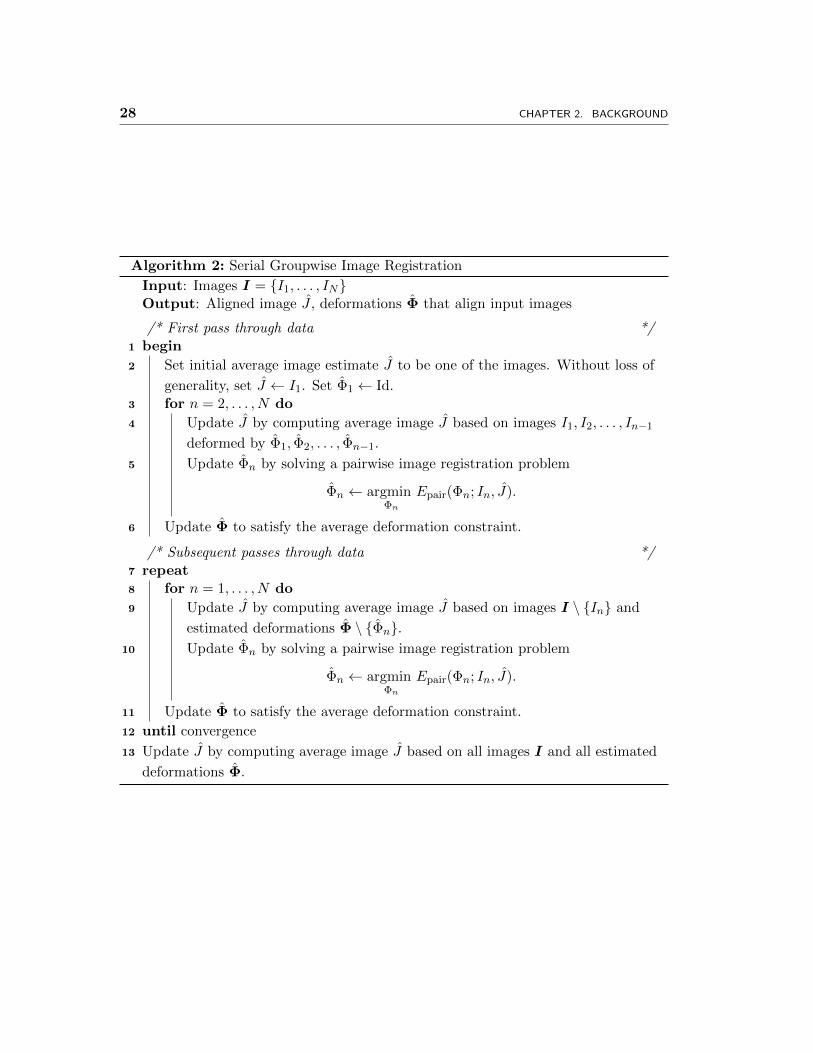
2.4.2 Serial Groupwise Image Registration
We outline in Alg. 2 a serial groupwise registration approach by Sabuncu et al. [31]
that essentially recomputes an average image before every pairwise registration and
can result in a sharper resulting average image J . Excluding the current image being
registered in line 9 is done to reduce bias in pairwise image registration from line 10 and
can be thought of as an implementation detail. Without excluding the current image
being registered, lines 7-12 of the algorithm can be viewed as doing coordinate ascent
for energy Egroup simply in a different order than in the parallel approach.
2.5 Finding Group-level Functional Brain Activations in fMRI
To determine what brain regions consistently activate due to a specific task such as
language processing or face recognition, we first need some way of measuring brain
activity. One way of doing this is to use fMRI, which will be the source of our data
in Chapter 4. We provide some fMRI basics before reviewing prior work on finding
group-level functional brain activations in fMRI.
FMRI is a widely used imaging modality for observing functional activity in the
brain. We specifically consider fMRI that uses the blood-oxygenation-level-dependent
(BOLD) magnetic resonance contrast [26]. BOLD fMRI is a non-invasive way to mea-
sure the blood oxygenation level in the brain, where local blood flow and local brain
metabolism are closely linked [30]. In particular, when neural activity occurs at a cer-
tain location in the brain, blood oxygenation level rises around that location, tapering
off after the neural activity subsides. As such, fMRI provides an indirect measure of
neural activity.
For this thesis, we treat fMRI preprocessing as a black box, referring the reader
to prior work [4, 16] for details on standard fMRI preprocessing and to the first three
chapters of [21] for an overview of fMRI analysis. The output of the black box, which
we treat as the observed fMRI data, consists of one 3D image per individual or sub-
ject, where each voxel has an intensity value roughly correlated with the voxel being
“activated” by a particular stimulus of interest, such as reading sentences. Assuming
the stimulus to be the same across a group of individuals, we seek to draw conclusions
28 CHAPTER 2. BACKGROUND
Algorithm 2: Serial Groupwise Image Registration
Input: Images I = I1, . . . , INOutput: Aligned image J , deformations Φ that align input images
/* First pass through data */1 begin
2 Set initial average image estimate J to be one of the images. Without loss of
generality, set J ← I1. Set Φ1 ← Id.3 for n = 2, . . . , N do
4 Update J by computing average image J based on images I1, I2, . . . , In−1
deformed by Φ1, Φ2, . . . , Φn−1.
5 Update Φn by solving a pairwise image registration problem
Φn ← argminΦn
Epair(Φn; In, J).
6 Update Φ to satisfy the average deformation constraint.
/* Subsequent passes through data */7 repeat8 for n = 1, . . . , N do
9 Update J by computing average image J based on images I \ In and
estimated deformations Φ \ Φn.10 Update Φn by solving a pairwise image registration problem
Φn ← argminΦn
Epair(Φn; In, J).
11 Update Φ to satisfy the average deformation constraint.
12 until convergence
13 Update J by computing average image J based on all images I and all estimated
deformations Φ.
Sec. 2.5. Finding Group-level Functional Brain Activations in fMRI 29
about how the group responds to the stimulus.
As mentioned in the introduction to this thesis, two types of variability pose chal-
lenges to accurately assessing the group response:
• Anatomical variability. Different subjects’ brains are anatomically different.
Thus, a popular procedure for obtaining the average group response is to first
align all subjects’ fMRI data to a common space, such as the Talairach space [32].
This involves aligning each individual’s fMRI data to a template brain [7].
• Functional variability. Even if we first aligned each subject’s brain into a com-
mon anatomically-normalized space so that anatomical structures line up perfectly,
when given a particular stimulus, different subjects experience brain activations
in different locations within the anatomically-normalized space.
After addressing anatomical variability by aligning images to a template brain, the
standard approach assumes voxel-wise correspondences across subjects, which means
that for a given voxel in the common space, different subjects’ data at that voxel
are assumed to be from the same location in the brain. Then the group’s functional
response at a voxel is taken to be essentially the average of the subjects’ fMRI data
at that voxel. This approach relies on the registration process being perfect and there
being no functional variability, neither of which is true [1, 17, 19].
Recent work addresses functional variability in different ways [31, 34, 39]. Thirion
et al. [34] identify contiguous regions, or parcels, of functional activation at the subject
level and then find parcel correspondences across subjects. While this approach yields
reproducible activation regions and provides spatial correspondences across subjects, its
bottom-up, rule-based nature does not incorporate a notion of a group template while
finding the correspondences. Instead, it builds a group template as a post-processing
step. As such, the model lacks a clear group-level interpretation of the estimated
parcels. In contrast, Xu et al. [39] use a spatial point process in a hierarchical Bayesian
model to describe functional activation regions. Their formulation accounts for vari-
able shape of activation regions and has an intuitive interpretation of group-level acti-
vations. However, since the model represents shapes using Gaussian mixture models,
functional regions of complex shape could require a large number of Gaussian compo-
nents. Lastly, Sabuncu et al. [31] sidestep finding functional region correspondences
altogether by estimating voxel-wise correspondences through groupwise registration of
functional activation maps from different subjects. This approach does not explicitly
model functional regions.
30 CHAPTER 2. BACKGROUND
In this thesis, we propose a novel way to characterize functional variability that
combines ideas from [31, 34, 39]. We model each subject’s activation map as a weighted
sum of group-level functional activation parcels that undergo a subject-specific defor-
mation. Similar to Xu et al. [39], we define a hierarchical generative model, but instead
of using a Gaussian mixture model to represent shapes, we represent each parcel as
an image, which allows for complex shapes. By explicitly modeling parcels, our model
yields parcel correspondences across subjects, similar to [34]. Second, we assume that
the template regions can deform to account for spatial variability of activation regions
across subjects. This involves using groupwise registration similar to [31] that is guided
by estimated group-level functional activation regions. We perform inference within
the proposed model using an algorithm similar to expectation-maximization (EM) [8]
and illustrate our method on the language system, which is known to have significant
functional variability [14].
Chapter 3
Probabilistic Deformation-Invariant
Sparse Coding
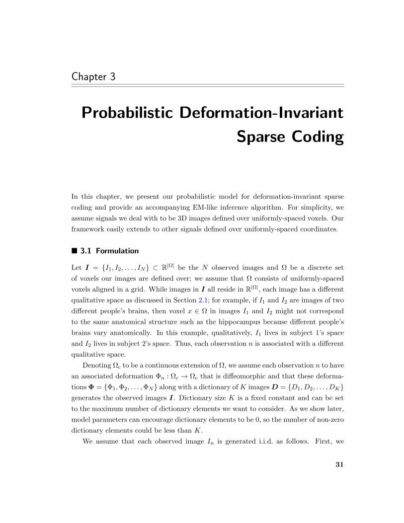
In this chapter, we present our probabilistic model for deformation-invariant sparse
coding and provide an accompanying EM-like inference algorithm. For simplicity, we
assume signals we deal with to be 3D images defined over uniformly-spaced voxels. Our
framework easily extends to other signals defined over uniformly-spaced coordinates.
3.1 Formulation
Let I = I1, I2, . . . , IN ⊂ R|Ω| be the N observed images and Ω be a discrete set
of voxels our images are defined over; we assume that Ω consists of uniformly-spaced
voxels aligned in a grid. While images in I all reside in R|Ω|, each image has a different
qualitative space as discussed in Section 2.1; for example, if I1 and I2 are images of two
different people’s brains, then voxel x ∈ Ω in images I1 and I2 might not correspond
to the same anatomical structure such as the hippocampus because different people’s
brains vary anatomically. In this example, qualitatively, I1 lives in subject 1’s space
and I2 lives in subject 2’s space. Thus, each observation n is associated with a different
qualitative space.
Denoting Ωc to be a continuous extension of Ω, we assume each observation n to have
an associated deformation Φn : Ωc → Ωc that is diffeomorphic and that these deforma-
tions Φ = Φ1,Φ2, . . . ,ΦN along with a dictionary of K imagesD = D1, D2, . . . , DKgenerates the observed images I. Dictionary size K is a fixed constant and can be set
to the maximum number of dictionary elements we want to consider. As we show later,
model parameters can encourage dictionary elements to be 0, so the number of non-zero
dictionary elements could be less than K.
We assume that each observed image In is generated i.i.d. as follows. First, we
31
32 CHAPTER 3. PROBABILISTIC DEFORMATION-INVARIANT SPARSE CODING
Dictionary
D1 D2 D3
1. Generate weights for each dictionary element, e.g., wn = (0.3, 1, 0).
2. Form weighted sum of dictionary elements with wn:
0.3 +1 +0 =
pre-image
Jn
D1 D2 D3
3. Deform pre-image and add noise:
noise
Jn Jn ©n 1 In
©n 1
Figure 3.1: Illustration of how our generative model produces observed image In for agiven dictionary of size K = 3.
draw weight vector wn ∈ RK where each scalar entry wnk is independently sampled
from distribution pw(·;λk). Then, we construct pre-image Jn =∑K
k=1wnkDk. The
observed image In = Jn Φ−1n + εn is the result of applying invertible deformation Φ−1
n
to pre-image Jn and adding white Gaussian noise εn with variance σ2. This generative
process is illustrated in Fig. 3.1 and defines the following joint probability distribution
over weight vector wn and observed image In for observation n:
p(In, wn|Φn,D;λ, σ2) =
[K∏k=1
pw(wnk;λk)
]N
(In;
K∑k=1
wnk(Dk Φ−1n ), σ2I|Ω|×|Ω|
),
(3.1)
where λ = λ1, λ2, . . . , λK.Our goal is to infer dictionary D and deformations Φ given a training set I of ob-
servations so that for future observations that have the same qualitative spaces as our
Sec. 3.1. Formulation 33
©
In
N
D
wnk
K
¸k
¾ 2
®, ¯, °,
Vmax, rmax
Figure 3.2: A probabilistic graphical model for our generative process.
training observations, we can treat the dictionary and observation-specific deformations
as fixed. Thus, the sparse linear combination weights are treated as latent variables dur-
ing training. Meanwhile, since we don’t know λ and σ2, we find maximum-likelihood es-
timates for these parameters. Mathematically, the resulting inference problem amounts
to solving the optimization problem
(D, Φ, λ, σ2)← argminD,Φ,λ,σ2
p(Φ,D|I;λ, σ2). (3.2)
For example, in our neuroimaging application, we learn a dictionary and deformations
from a training set that comes from N subjects, and we validate on held-out data from
the same subjects. At the end of this chapter, we briefly discuss several extensions:
(i) estimating sparse linear combination weights w in addition to (D,Φ,λ, σ2), which
is an easier problem as the weights are not treated as latent variables; (ii) having
deformations be both observation-specific and dictionary-element specific; (iii) handling
new observations that have qualitative spaces that aren’t in the training observations;
and (iv) incorporating ground truth segmentations for supervised learning.
3.1.1 Model Parameters
We treat each deformation Φn as a random parameter with prior distribution pΦ(·),which can also be viewed as regularizing each deformation to prevent overfitting. Choice
of the deformation prior allows us to leverage existing image registration algorithms;
specifically, our inference algorithm described in Section 3.2 works with any registration
34 CHAPTER 3. PROBABILISTIC DEFORMATION-INVARIANT SPARSE CODING
algorithm that minimizes an energy of the form
E(Φ; I, J) =1
2σ2‖I Φ− J‖22 − log pΦ(Φ), (3.3)
for moving image I ∈ R|Ω| that undergoes deformation Φ and fixed image J ∈ R|Ω|,where Φ is restricted to be in a subset of diffeomorphisms mapping Ωc to Ωc. To
prevent spatial drift of the dictionary elements during inference, we add a constraint
that the average deformation be identity where we define the average deformation to
be Φ1 Φ2 · · · ΦN . The overall prior on deformations Φ is thus
p(Φ) =
[N∏n=1
pΦ(Φn)
]· 1 Φ1 · · · ΦN = Id , (3.4)
where 1· is the indicator function that equals 1 when its argument is true and equals 0
otherwise.
Our inference algorithm depends on the following volume change condition on each
deformation Φn: Letting |JΦn(x)| denote the Jacobian determinant of Φn evaluated
at voxel x, we require |JΦn(x)| ≤ φmax for all x ∈ Ω and for some pre-specified con-
stant φmax ≥ 1. As |JΦn(x)| is the volume change ratio for voxel x due to deforma-
tion Φn, the volume change condition can be thought of as a constraint on how much
deformation Φn is allowed to shrink or expand part of an image (e.g., if Φn is identity,
then |JΦn(x)| = 1 for all x ∈ Ω). Rather than folding the volume change condition in
as a constraint on each deformation Φn, we instead just require that prior pΦ be chosen
so that this condition is satisfied. This condition is essentially a regularity condition,
showing up in the derivation for the inference algorithm and also resulting in a rescaling
of images when estimating a deformation to align them during inference.
We also treat each dictionary element Dk as a random parameter. Similar to the
sparse coding setup in Section 2.2, we resolve the discrepancy between scaling Dk and
inversely scaling wnk by constraining each dictionary element Dk to have bounded `2
norm: ‖Dk‖2 ≤ 1. To encourage sparsity and smoothness, we introduce `1 and MRF
penalties. To encourage each dictionary element to be a localized basis, we require each
Dk to have spatial support (i.e., the set of voxels for which Dk is non-zero) contained
within an ellipsoid of pre-specified (maximum) volume Vmax and maximum semi-axis
length rmax; notationally, we denote the set of ellipsoids satisfying these two conditions
as E(Vmax, rmax).1 Finally, to discourage overlap between different dictionary elements,
1The semi-axis constraint ensures that we don’t have oblong ellipsoids that satisfy the volume con-
Sec. 3.1. Formulation 35
we place an `1 penalty on the element-wise product between every pair of distinct
dictionary elements. Formally,
p(D;α, β, γ, Vmax, rmax) ∝ exp
−K∑k=1
(α‖Dk‖1 +β
2D>k LDk)− γ
∑k 6=`‖Dk D`‖1
·K∏k=1
1
‖Dk‖2 ≤ 1,
∃Ek ∈ E(Vmax, rmax) s.t. Ek ⊇ support(Dk)
,
(3.5)
where hyperparameters α, β, γ, Vmax, and rmax are positive constants, “” denotes
element-wise multiplication, and L is the graph Laplacian for a grid graph defined over
voxels Ω. As eq. (3.5) suggests, the spatial support of different dictionary elements may
be contained by different ellipsoids from E(Vmax, rmax).
Other model parameters are treated as non-random: λ parameterizes distributions
pw(·;λk) for each k, and σ2 is the variance of the Gaussian noise. We use MAP esti-
mation for D and Φ and ML estimation for λ and σ2. Cross-validation can be used
to select hyperparameters α, β, and γ. Hyperparameters Vmax and rmax are set to val-
ues representative for the maximum spatial support we want our dictionary elements
to have.
With the above model parameters, the full joint distribution for our model becomes
p(I,w,Φ,D;λ, σ2)
∝ p(D)N∏n=1
pΦ(Φn)
[K∏k=1
pw(wnk;λk)
]N
(In;
K∑k=1
wnk(Dk Φ−1n ), σ2I|Ω|×|Ω|
),
(3.6)
where average deformation Φ1 · · · Φn is identity and p(D) refers to eq. (3.5); we omit
writing out hyperparameters α, β, γ, Vmax, and rmax for notational convenience and
since we will not be maximizing over these variables with our inference algorithm. A
probabilistic graphical model representation for this distribution is given in Fig. 3.2.
straint yet have, for example, one semi-axis length extremely large and all others close to 0. Thisconstraint also allows us to quickly find the spatial support of each dictionary element during inference.
36 CHAPTER 3. PROBABILISTIC DEFORMATION-INVARIANT SPARSE CODING
3.1.2 Relation to Sparse Coding
With λ1 = · · · = λK = λ for some constant λ > 0, a Laplace prior for pw, no defor-
mations (i.e., deformations are all identity), and a uniform prior for each Dk on the
unit `2 disk (i.e., α = β = γ = 0 and Vmax = rmax = ∞), we obtain the probabilistic
sparse coding model (2.7) discussed in Section 2.2. We extend sparse coding by allow-
ing dictionary elements to undergo observation-specific deformations. We estimate a
set of deformations Φ and the distribution for latent weights w in addition to learn-
ing the dictionary D. Effectively, we recover dictionary elements invariant to “small”
deformations, where the “size” of a deformation is governed by the deformation prior.
Our deformation-invariant sparse coding model can be interpreted as mapping each
observation In ∈ R|Ω| to a pair (wn,Φn), where wn ∈ RK and function Φn maps Ωc to Ωc.
If K = o(|Ω|) and Φn has a sparse description of size o(|Ω|), then deformation-invariant
sparse coding can be interpreted as performing a nonlinear dimensionality reduction.
Specifically for deformations, the subset of diffeomorphisms we work with could give Φn
a sparse description. For example, if Φn is an invertible affine transformation, then it
is fully characterized by a small matrix. Recent work by Durrleman et al. [11] param-
eterizes diffeomorphisms by a sparse set of control points with accompanying velocity
vectors, which can represent more fine-grain deformations than affine transformations.
3.2 Inference
We use an EM-like algorithm2 to estimate deformations Φ, dictionary D, and non-
random model parameters (λ, σ2). Appendix A contains detailed derivations of the
algorithm. To make computation tractable, a key ingredient of the E-step is to approx-
imate posterior distribution p(w|I,Φ,D;λ, σ2) with a fully-factored distribution
q(w;ψ) =N∏n=1
K∏k=1
qw(wnk;ψnk), (3.7)
where distribution qw(·;ψnk) is parameterized by ψnk. Importantly, we keep track of the
first and second moments of each latent weight wnk, denoted as 〈wnk〉 , Eqw [wnk|I, Φ, D]
and 〈w2nk〉 , Eqw [w2
nk|I, Φ, D], where qw = qw(·; ψnk); collectively the first moments
are denoted as 〈w〉 and the second moments as 〈w2〉. Effectively the E-step involves
computing these moments, which are just expectations. The resulting algorithm is
2Due to approximations we make, the algorithm is strictly speaking not EM or even generalized EM.
Sec. 3.2. Inference 37
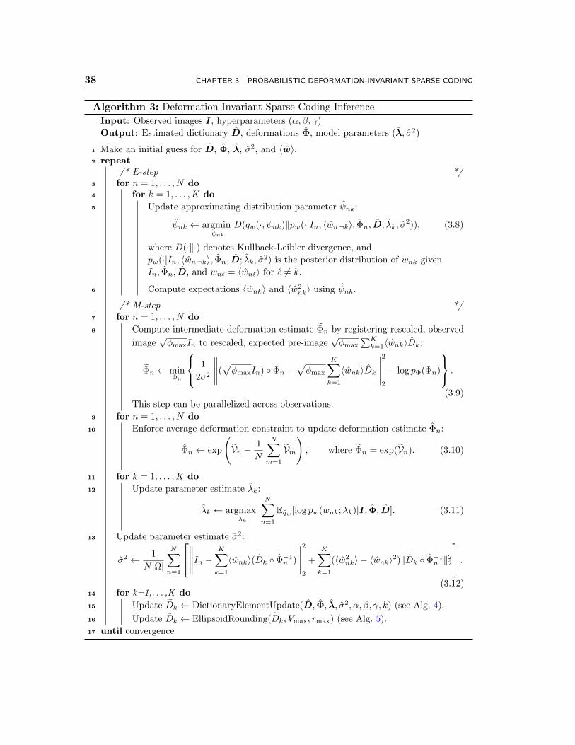
summarized in Alg. 3.
We elaborate on how each dictionary element estimate Dk is updated. By holding
all other estimated variables constant, updating Dk amounts to numerically minimizing
the following energy:
E(Dk)
=1
2σ2
N∑n=1
∑x∈Ω
|JΦn(x)|
(In(Φn(x))−K∑`=1
〈wn`〉D`(x)
)2
+ (〈w2nk〉 − 〈wnk〉2)D2
k(x)
+ α‖Dk‖1 +
β
2D>k LDk + γ
∑` 6=k‖Dk D`‖1, (3.13)
where Dk satisfies ‖Dk‖2 ≤ 1 and is contained within an ellipsoid of volume Vmax. This
procedure allows for a dictionary element to converge to 0, which would suggest the
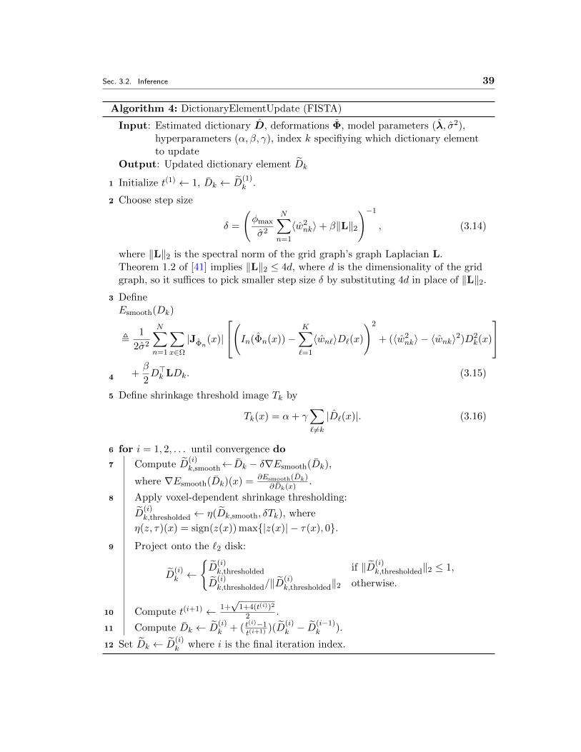
dictionary element to be extraneous. As for how the numerical minimization is carried
out, we first solve a convex relaxation that omits the ellipsoid constraint. The resulting
convex problem can be efficiently solved using the fast iterative shrinkage-thresholding
algorithm (FISTA) [3], which we specialize for minimizing E(Dk) subject to ‖Dk‖2 ≤ 1
in Alg. 4. Next, we reintroduce the ellipsoid constraint via the rounding scheme given
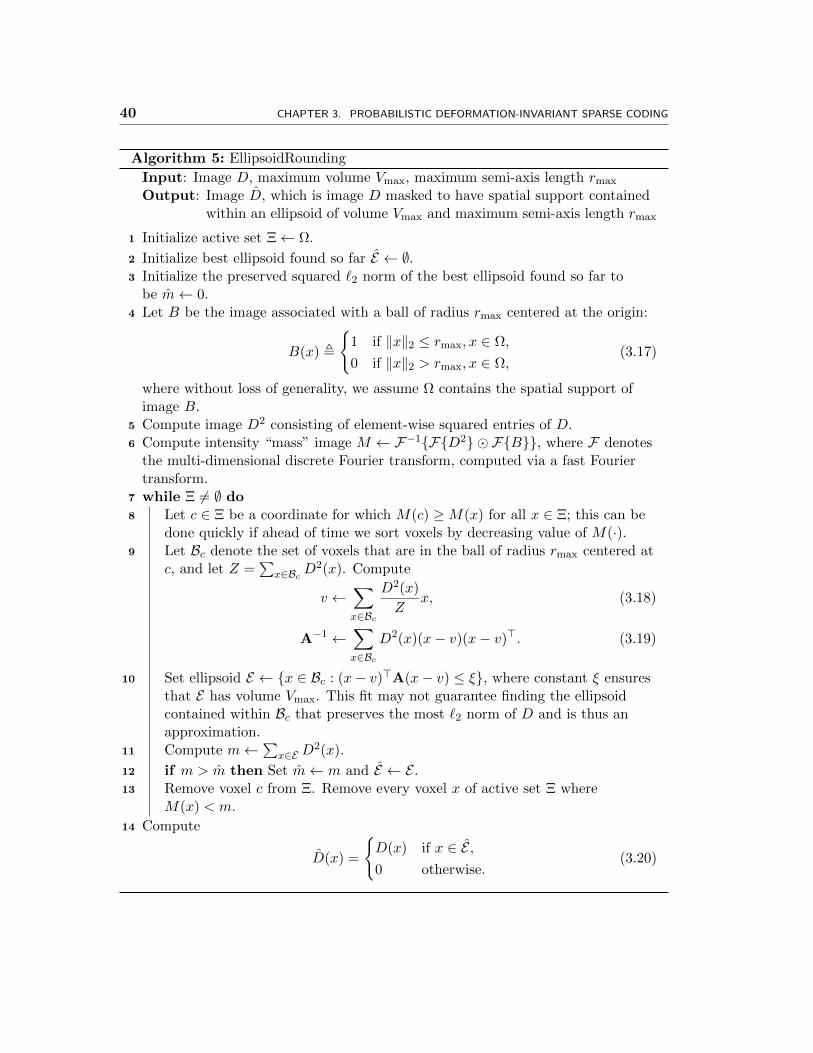
in Alg. 5. The rounding scheme basically masks the output of the convex program’s
solution Dk to an ellipsoid of maximum volume Vmax and maximum semi-axis length
rmax such that the intensities inside the ellipsoid are large in terms of `2 norm. A sketch
of how this ellipsoid is found:
1. For every ball Bc of radius rmax with center c ∈ Ω, compute “mass” image M(c) =∑x∈Bc |Dk(x)|2. Basically M(c) gives us a measure of how much intensity “mass”
is preserved by restricting image Dk to ball Bc.
2. Rank all voxels c1, . . . , c|Ω| in Ω so that M(c1) ≥M(c2) ≥ · · · ≥M(c|Ω|).
3. For i = 1, . . . , |Ω|: Fit an ellipsoid to voxels in Bci that preserves as much `2 norm
as possible in Dk. Keep track of which ellipsoid found so far preserves the most
amount of intensity, and break out of the for loop as soon as our best ellipsoid found
so far preserves more intensity than any of the remaining balls Bci+1 , . . . ,Bc|Ω| .
The first step here can actually be computed efficiently with the help of a fast Fourier
transform. To fit an ellipsoid for the third step, we use an approximation that may not
yield the best possible ellipsoid within a ball of radius rmax.
38 CHAPTER 3. PROBABILISTIC DEFORMATION-INVARIANT SPARSE CODING
Algorithm 3: Deformation-Invariant Sparse Coding Inference
Input: Observed images I, hyperparameters (α, β, γ)
Output: Estimated dictionary D, deformations Φ, model parameters (λ, σ2)
1 Make an initial guess for D, Φ, λ, σ2, and 〈w〉.2 repeat
/* E-step */3 for n = 1, . . . , N do4 for k = 1, . . . ,K do
5 Update approximating distribution parameter ψnk:
ψnk ← argminψnk
D(qw(·;ψnk)‖pw(·|In, 〈wn¬k〉, Φn, D; λk, σ2)), (3.8)
where D(·‖·) denotes Kullback-Leibler divergence, and
pw(·|In, 〈wn¬k〉, Φn, D; λk, σ2) is the posterior distribution of wnk given
In, Φn, D, and wn` = 〈wn`〉 for ` 6= k.
6 Compute expectations 〈wnk〉 and 〈w2nk〉 using ψnk.
/* M-step */7 for n = 1, . . . , N do
8 Compute intermediate deformation estimate Φn by registering rescaled, observed
image√φmaxIn to rescaled, expected pre-image
√φmax
∑Kk=1〈wnk〉Dk:
Φn ← minΦn
1
2σ2
∥∥∥∥∥(√φmaxIn) Φn −
√φmax
K∑k=1
〈wnk〉Dk
∥∥∥∥∥2
2
− log pΦ(Φn)
.
(3.9)This step can be parallelized across observations.
9 for n = 1, . . . , N do
10 Enforce average deformation constraint to update deformation estimate Φn:
Φn ← exp
(Vn −
1
N
N∑m=1
Vm
), where Φn = exp(Vn). (3.10)
11 for k = 1, . . . ,K do
12 Update parameter estimate λk:
λk ← argmaxλk
N∑n=1
Eqw [log pw(wnk;λk)|I, Φ, D]. (3.11)
13 Update parameter estimate σ2:
σ2 ← 1
N |Ω|
N∑n=1
∥∥∥∥∥In −K∑k=1
〈wnk〉(Dk Φ−1n )
∥∥∥∥∥2
2
+
K∑k=1
(〈w2nk〉 − 〈wnk〉2)‖Dk Φ−1
n ‖22
.(3.12)
14 for k=1,. . . ,K do
15 Update Dk ← DictionaryElementUpdate(D, Φ, λ, σ2, α, β, γ, k) (see Alg. 4).
16 Update Dk ← EllipsoidRounding(Dk, Vmax, rmax) (see Alg. 5).
17 until convergence
Sec. 3.2. Inference 39
Algorithm 4: DictionaryElementUpdate (FISTA)
Input: Estimated dictionary D, deformations Φ, model parameters (λ, σ2),hyperparameters (α, β, γ), index k specifiying which dictionary elementto update
Output: Updated dictionary element Dk
1 Initialize t(1) ← 1, Dk ← D(1)k .
2 Choose step size
δ =
(φmax
σ2
N∑n=1
〈w2nk〉+ β‖L‖2
)−1
, (3.14)
where ‖L‖2 is the spectral norm of the grid graph’s graph Laplacian L.Theorem 1.2 of [41] implies ‖L‖2 ≤ 4d, where d is the dimensionality of the gridgraph, so it suffices to pick smaller step size δ by substituting 4d in place of ‖L‖2.
3 DefineEsmooth(Dk)
,1
2σ2
N∑n=1
∑x∈Ω
|JΦn(x)|
(In(Φn(x))−K∑`=1
〈wn`〉D`(x)
)2
+ (〈w2nk〉 − 〈wnk〉2)D2
k(x)
+β
2D>k LDk. (3.15)4
5 Define shrinkage threshold image Tk by
Tk(x) = α+ γ∑`6=k|D`(x)|. (3.16)
6 for i = 1, 2, . . . until convergence do
7 Compute D(i)k,smooth←Dk − δ∇Esmooth(Dk),
where ∇Esmooth(Dk)(x) = ∂Esmooth(Dk)∂Dk(x)
.
8 Apply voxel-dependent shrinkage thresholding:
D(i)k,thresholded ← η(Dk,smooth, δTk), where
η(z, τ)(x) = sign(z(x)) max|z(x)| − τ(x), 0.
9 Project onto the `2 disk:
D(i)k ←
D
(i)k,thresholded if ‖D(i)
k,thresholded‖2 ≤ 1,
D(i)k,thresholded/‖D
(i)k,thresholded‖2 otherwise.
10 Compute t(i+1) ← 1+√
1+4(t(i))2
2 .
11 Compute Dk ← D(i)k + ( t
(i)−1t(i+1) )(D
(i)k − D
(i−1)k ).
12 Set Dk ← D(i)k where i is the final iteration index.
40 CHAPTER 3. PROBABILISTIC DEFORMATION-INVARIANT SPARSE CODING
Algorithm 5: EllipsoidRounding
Input: Image D, maximum volume Vmax, maximum semi-axis length rmax
Output: Image D, which is image D masked to have spatial support containedwithin an ellipsoid of volume Vmax and maximum semi-axis length rmax
1 Initialize active set Ξ← Ω.
2 Initialize best ellipsoid found so far E ← ∅.3 Initialize the preserved squared `2 norm of the best ellipsoid found so far to
be m← 0.4 Let B be the image associated with a ball of radius rmax centered at the origin:
B(x) ,
1 if ‖x‖2 ≤ rmax, x ∈ Ω,
0 if ‖x‖2 > rmax, x ∈ Ω,(3.17)
where without loss of generality, we assume Ω contains the spatial support ofimage B.
5 Compute image D2 consisting of element-wise squared entries of D.6 Compute intensity “mass” image M ← F−1FD2 FB, where F denotes
the multi-dimensional discrete Fourier transform, computed via a fast Fouriertransform.
7 while Ξ 6= ∅ do8 Let c ∈ Ξ be a coordinate for which M(c) ≥M(x) for all x ∈ Ξ; this can be
done quickly if ahead of time we sort voxels by decreasing value of M(·).9 Let Bc denote the set of voxels that are in the ball of radius rmax centered at
c, and let Z =∑
x∈Bc D2(x). Compute
v ←∑x∈Bc
D2(x)
Zx, (3.18)
A−1 ←∑x∈Bc
D2(x)(x− v)(x− v)>. (3.19)
10 Set ellipsoid E ← x ∈ Bc : (x− v)>A(x− v) ≤ ξ, where constant ξ ensuresthat E has volume Vmax. This fit may not guarantee finding the ellipsoidcontained within Bc that preserves the most `2 norm of D and is thus anapproximation.
11 Compute m←∑
x∈E D2(x).
12 if m > m then Set m← m and E ← E .13 Remove voxel c from Ξ. Remove every voxel x of active set Ξ where
M(x) < m.
14 Compute
D(x) =
D(x) if x ∈ E ,0 otherwise.
(3.20)
Sec. 3.2. Inference 41
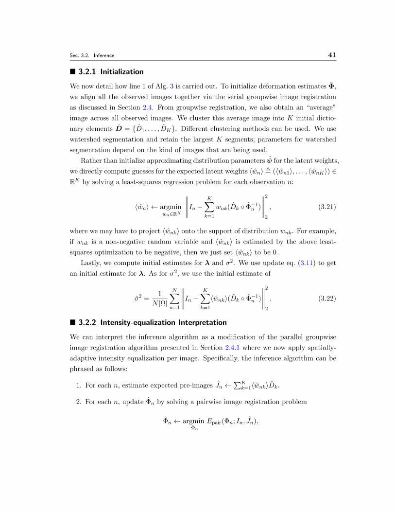
3.2.1 Initialization
We now detail how line 1 of Alg. 3 is carried out. To initialize deformation estimates Φ,
we align all the observed images together via the serial groupwise image registration
as discussed in Section 2.4. From groupwise registration, we also obtain an “average”
image across all observed images. We cluster this average image into K initial dictio-
nary elements D = D1, . . . , DK. Different clustering methods can be used. We use
watershed segmentation and retain the largest K segments; parameters for watershed
segmentation depend on the kind of images that are being used.
Rather than initialize approximating distribution parameters ψ for the latent weights,
we directly compute guesses for the expected latent weights 〈wn〉 , (〈wn1〉, . . . , 〈wnK〉) ∈RK by solving a least-squares regression problem for each observation n:
〈wn〉 ← argminwn∈RK
∥∥∥∥∥In −K∑k=1
wnk(Dk Φ−1n )
∥∥∥∥∥2
2
, (3.21)
where we may have to project 〈wnk〉 onto the support of distribution wnk. For example,
if wnk is a non-negative random variable and 〈wnk〉 is estimated by the above least-
squares optimization to be negative, then we just set 〈wnk〉 to be 0.
Lastly, we compute initial estimates for λ and σ2. We use update eq. (3.11) to get
an initial estimate for λ. As for σ2, we use the initial estimate of
σ2 =1
N |Ω|
N∑n=1
∥∥∥∥∥In −K∑k=1
〈wnk〉(Dk Φ−1n )
∥∥∥∥∥2
2
. (3.22)
3.2.2 Intensity-equalization Interpretation
We can interpret the inference algorithm as a modification of the parallel groupwise
image registration algorithm presented in Section 2.4.1 where we now apply spatially-
adaptive intensity equalization per image. Specifically, the inference algorithm can be
phrased as follows:
1. For each n, estimate expected pre-images Jn ←∑K
k=1〈wnk〉Dk.
2. For each n, update Φn by solving a pairwise image registration problem
Φn ← argminΦn
Epair(Φn; In, Jn),

42 CHAPTER 3. PROBABILISTIC DEFORMATION-INVARIANT SPARSE CODING
which can be done in parallel across n = 1, 2, . . . , N .
3. Update Φ to satisfy the average deformation constraint.
4. Update the estimates for D, λ, and σ2.
The expected pre-image for observation n allows each dictionary element to have a
different weight, which means that we adjust the intensity of the expected pre-image
by different amounts where different dictionary elements appear.
3.3 Extensions
We remark on a few possible extensions of our model.
• Estimating sparse linear combination weights instead of treating them as latent :
Regular sparse coding actually does not treat the weights as latent. By estimating
weights instead, our inference algorithm would actually become simpler since no
variational approximating distribution q over latent weights is needed. For exam-
ple, if the prior on weights pw is a Laplace distribution with the same parameter λ
across all dictionary elements, then the E-step becomes an instance of Lasso:
minwn∈RK
1
2σ2
∥∥∥∥∥In −K∑k=1
wnk(Dk Φ−1n )
∥∥∥∥∥2
2
+ λ‖wn‖1. (3.23)
Moreover, the volume change condition can actually be dropped since it was in-
troduced to determine which image is treated as fixed and which is treated as
moving when updating each deformation. Specifically, as shown in eq. (A.5) in
Appendix A, there is a term involving ‖Dk Φ−1n ‖22 that is present due to the
weights being latent and that would require modifying off-the-shelf image regis-
tration algorithms to account for it. Introducing the volume change condition and
making the expected pre-image the fixed image instead of the moving image allows
us to essentially get rid of this term when updating each deformation. However,
with weights that are not latent, we could treat the expected pre-image as the
moving image.
• Having deformations that are both observation-specific and dictionary-element-
specific: Our deformations are observation-specific, and depending on the subset of
diffeomorphisms we allow, observation-specific deformations could already provide
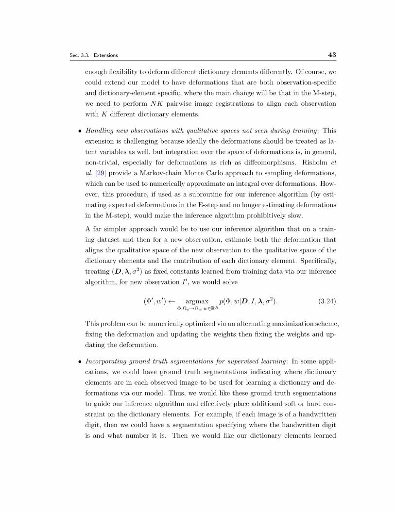
Sec. 3.3. Extensions 43
enough flexibility to deform different dictionary elements differently. Of course, we
could extend our model to have deformations that are both observation-specific
and dictionary-element specific, where the main change will be that in the M-step,
we need to perform NK pairwise image registrations to align each observation
with K different dictionary elements.
• Handling new observations with qualitative spaces not seen during training : This
extension is challenging because ideally the deformations should be treated as la-
tent variables as well, but integration over the space of deformations is, in general,
non-trivial, especially for deformations as rich as diffeomorphisms. Risholm et
al. [29] provide a Markov-chain Monte Carlo approach to sampling deformations,
which can be used to numerically approximate an integral over deformations. How-
ever, this procedure, if used as a subroutine for our inference algorithm (by esti-
mating expected deformations in the E-step and no longer estimating deformations
in the M-step), would make the inference algorithm prohibitively slow.
A far simpler approach would be to use our inference algorithm that on a train-
ing dataset and then for a new observation, estimate both the deformation that
aligns the qualitative space of the new observation to the qualitative space of the
dictionary elements and the contribution of each dictionary element. Specifically,
treating (D,λ, σ2) as fixed constants learned from training data via our inference
algorithm, for new observation I ′, we would solve
(Φ′, w′)← argmaxΦ:Ωc→Ωc, w∈RK
p(Φ, w|D, I,λ, σ2). (3.24)
This problem can be numerically optimized via an alternating maximization scheme,
fixing the deformation and updating the weights then fixing the weights and up-
dating the deformation.
• Incorporating ground truth segmentations for supervised learning : In some appli-
cations, we could have ground truth segmentations indicating where dictionary
elements are in each observed image to be used for learning a dictionary and de-
formations via our model. Thus, we would like these ground truth segmentations
to guide our inference algorithm and effectively place additional soft or hard con-
straint on the dictionary elements. For example, if each image is of a handwritten
digit, then we could have a segmentation specifying where the handwritten digit
is and what number it is. Then we would like our dictionary elements learned
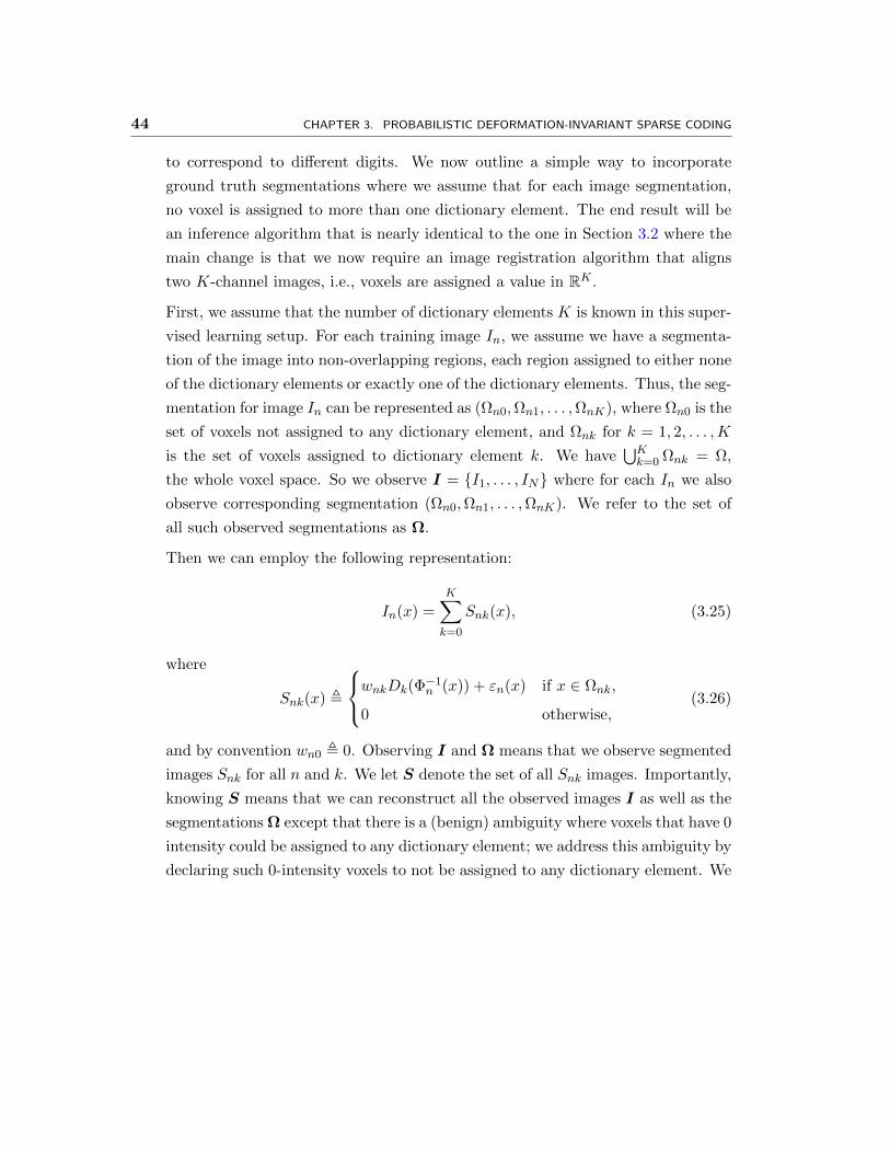
44 CHAPTER 3. PROBABILISTIC DEFORMATION-INVARIANT SPARSE CODING
to correspond to different digits. We now outline a simple way to incorporate
ground truth segmentations where we assume that for each image segmentation,
no voxel is assigned to more than one dictionary element. The end result will be
an inference algorithm that is nearly identical to the one in Section 3.2 where the
main change is that we now require an image registration algorithm that aligns
two K-channel images, i.e., voxels are assigned a value in RK .
First, we assume that the number of dictionary elements K is known in this super-
vised learning setup. For each training image In, we assume we have a segmenta-
tion of the image into non-overlapping regions, each region assigned to either none
of the dictionary elements or exactly one of the dictionary elements. Thus, the seg-
mentation for image In can be represented as (Ωn0,Ωn1, . . . ,ΩnK), where Ωn0 is the
set of voxels not assigned to any dictionary element, and Ωnk for k = 1, 2, . . . ,K
is the set of voxels assigned to dictionary element k. We have⋃Kk=0 Ωnk = Ω,
the whole voxel space. So we observe I = I1, . . . , IN where for each In we also
observe corresponding segmentation (Ωn0,Ωn1, . . . ,ΩnK). We refer to the set of
all such observed segmentations as Ω.
Then we can employ the following representation:
In(x) =K∑k=0
Snk(x), (3.25)
where
Snk(x) ,
wnkDk(Φ−1n (x)) + εn(x) if x ∈ Ωnk,
0 otherwise,(3.26)
and by convention wn0 , 0. Observing I and Ω means that we observe segmented
images Snk for all n and k. We let S denote the set of all Snk images. Importantly,
knowing S means that we can reconstruct all the observed images I as well as the
segmentations Ω except that there is a (benign) ambiguity where voxels that have 0
intensity could be assigned to any dictionary element; we address this ambiguity by
declaring such 0-intensity voxels to not be assigned to any dictionary element. We
Sec. 3.3. Extensions 45
now consider a probabilistic model that treats segmented images S as observations:
p(S,w|Φ,D;λ, σ2)
=N∏n=1
[K∏k=1
p(wnk;λk)
] K∏k=1
∏x∈Ωk
N (Snk(x);wnkDk(Φ−1n (x)), σ2)
. (3.27)
We can place priors on sparse linear combination weights, deformations, and the
dictionary as in Section 3.1. Treating weights w as latent and inferring defor-
mations Φ, dictionary D, and parameters (λ, σ2) can be done with an algorithm
similar the one in Section 3.2. The main change is that to update estimate Φn,
we align K-channel image SnkKk=1 with K-channel image 〈wnk〉DkKk=1. If we
know that each image has exactly one dictionary element present (e.g., each image
is of a handwritten digit), then we just need single-channel image registration.
Specifically for handwritten digits, the inference algorithm would just align all
the images of 1’s to obtain a dictionary element or template for digit 1 and then
repeat this for all the other digits. Then for a new observed image, we estimate
the contribution of each dictionary element, where one way to classify the obser-
vation is to declare the most likely digit to be the dictionary element with the
highest contribution, which essentially amounts to aligning the observed image to
each dictionary element and deciding which dictionary element provides the best
alignment. Such deformable template models are not new and have been used for
handwritten digit and face recognition [18, 24].
A general, probabilistic framework for deformable template models for object
recognition is presented in [15], which relies on choosing a dictionary of parts
that make sense for the recognition task (e.g., having the parts be eyes, a nose,
etc. for face recognition). In contrast, our model is presented in the context of
unsupervised learning.

46 CHAPTER 3. PROBABILISTIC DEFORMATION-INVARIANT SPARSE CODING
Chapter 4
Modeling Spatial Variability of
Functional Patterns in the Brain
We seek group-level functional units (i.e., parcels) in the brain that activate due to
language processing by representing them as dictionary elements with deformation-
invariant sparse coding. After instantiating our inference algorithm to a specific choice
of priors for sparse linear combination weights and deformations, this chapter showcases
results on synthetic data and fMRI activation maps from a language fMRI study.
4.1 Instantiation to fMRI Analysis
We specialize our model in Chapter 3 for fMRI analysis. First and foremost, obser-
vations directly correspond to different subjects; image In gives us a brain activa-
tion map for subject n. Since we look for positive activation due to functional stim-
uli probing lexical and structural language processing, it suffices to restrict weights
w in our model to be non-negative. We place i.i.d. exponential priors on each wnk
to encourage sparsity: pw(wnk;λk) = λke−λkwnk where wnk ≥ 0 and λk > 0. We
use log-domain diffeomorphic Demons registration [37] to estimate deformations Φ:
pΦ(Φn) ∝ exp−LogDiffDemonsReg(Φn), where LogDiffDemonsReg(·) is given by
eq. (2.11). Combining these priors for weights w and deformations Φ with eqs. (3.1),
(3.4), and (3.5) yields the full joint distribution:
p(I,w,Φ,D;λ, σ2)
∝ p(D)N∏n=1
exp(−LogDiffDemonsReg(Φn))[K∏k=1
λke−λkwnk
]N
(In;
K∑k=1
wnk(Dk Φ−1n ), σ2I|Ω|×|Ω|
), (4.1)
47
48 CHAPTER 4. MODELING SPATIAL VARIABILITY OF FUNCTIONAL PATTERNS IN THE BRAIN
where weights w are non-negative, the average deformation Φ1 · · · Φn is identity, and
p(D) refers to eq. (3.5). As before, prior p(D) depends on hyperparameters α, β, γ,
Vmax, and rmax, which we suppress for notational convenience. While we don’t place a
hard constraint that each dictionary element Dk be a parcel, i.e., have spatial support
that is a contiguous region, we empirically find our ellipsoid constraint to produce
dictionary elements that are parcels provided that α, Vmax, and rmax are not too large.
Meanwhile, despite treating log-domain diffeomorphic Demons registration as a
black box, we acknowledge the importance of choosing registration parameters to pre-
vent data overfitting. These parameters largely depend on the images used for registra-
tion. In our experiments, we use default parameters from the ITK implementation of
log-domain diffeomorphic Demons registration [10] except that we increase the variance
of the isotropic Gaussian kernel used for smoothing the deformation’s velocity field from
(1.5 voxels)2 to (2.5 voxels)2 and decrease the maximum length of the velocity update
vector from 2 voxels to 1 voxel.
Given our choice of priors on weights and deformations, we can now extract explicit
update rules for optimization problems (3.8) and (3.11) in the EM-like algorithm of
Chapter 3 while using log-domain Demons registration to solve (3.9). Approximating
posterior probability distribution q for latent weights w is set to
q(w;µ,ν) =
N∏n=1
K∏k=1
N+(wnk;µnk, νnk), (4.2)
whereN+(·;µnk, νnk) is the probability density of the normal distribution with mean µnk
and variance νnk restricted to have non-negative support, i.e., the positive normal distri-
bution. Thus, ψnk from eq. (3.7) is given by ψnk = (µnk, νnk). Deferring derivations to
Appendix B, we summarize the resulting inference algorithm in Alg. 6, where we denote
〈wnk〉 , Eq[wnk|I, Φ, D], 〈w2nk〉 , Eq[w2
nk|I, Φ, D], and q to be distribution (4.2) pa-
rameterized by µ and ν. The initialization procedure expands on that of Section 3.2.1
and is outlined in Alg. 7. Before running the inference algorithm, we must set the
hyperparameters. As mentioned previously, hyperparameters Vmax and rmax have intu-
itive interpretations and are hand-set based on the maximum spatial support size we
would like each dictionary element to have. Thus, our discussion of hyperparameter
tuning will focus on choosing α, β, and γ.
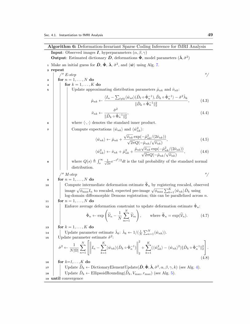
Sec. 4.1. Instantiation to fMRI Analysis 49
Algorithm 6: Deformation-Invariant Sparse Coding Inference for fMRI Analysis
Input: Observed images I, hyperparameters (α, β, γ)
Output: Estimated dictionary D, deformations Φ, model parameters (λ, σ2)
1 Make an initial guess for D, Φ, λ, σ2, and 〈w〉 using Alg. 7.2 repeat
/* E-step */3 for n = 1, . . . , N do4 for k = 1, . . . ,K do5 Update approximating distribution parameters µnk and νnk:
µnk ←〈In −
∑` 6=k〈wn`〉(D` Φ−1
n ), Dk Φ−1n 〉 − σ2λk
‖Dk Φ−1n ‖22
, (4.3)
νnk ←σ2
‖Dk Φ−1n ‖22
, (4.4)
6 where 〈·, ·〉 denotes the standard inner product.
7 Compute expectations 〈wnk〉 and 〈w2nk〉:
〈wnk〉 ← µnk +
√νnk exp(−µ2
nk/(2νnk))√2πQ(−µnk/
√νnk)
, (4.5)
〈w2nk〉 ← νnk + µ2
nk +µnk√νnk exp(−µ2
nk/(2νnk))√2πQ(−µnk/
√νnk)
, (4.6)
8 where Q(s) ,∫∞s
1√2πe−t
2/2dt is the tail probability of the standard normal
distribution.
/* M-step */9 for n = 1, . . . , N do
10 Compute intermediate deformation estimate Φn by registering rescaled, observed
image√φmaxIn to rescaled, expected pre-image
√φmax
∑Kk=1〈wnk〉Dk using
log-domain diffeomorphic Demons registration; this can be parallelized across n.
11 for n = 1, . . . , N do
12 Enforce average deformation constraint to update deformation estimate Φn:
Φn ← exp
(Vn −
1
N
N∑m=1
Vm
), where Φn = exp(Vn). (4.7)
13 for k = 1, . . . ,K do
14 Update parameter estimate λk: λk ← 1/( 1N
∑Nn=1〈wnk〉).
15 Update parameter estimate σ2:
σ2 ← 1
N |Ω|
N∑n=1
∥∥∥∥∥In −K∑k=1
〈wnk〉(Dk Φ−1n )
∥∥∥∥∥2
2
+
K∑k=1
(〈w2nk〉 − 〈wnk〉2)‖Dk Φ−1
n ‖22
.(4.8)
16 for k=1,. . . ,K do
17 Update Dk ← DictionaryElementUpdate(D, Φ, λ, σ2, α, β, γ, k) (see Alg. 4).
18 Update Dk ← EllipsoidRounding(Dk, Vmax, rmax) (see Alg. 5).
19 until convergence
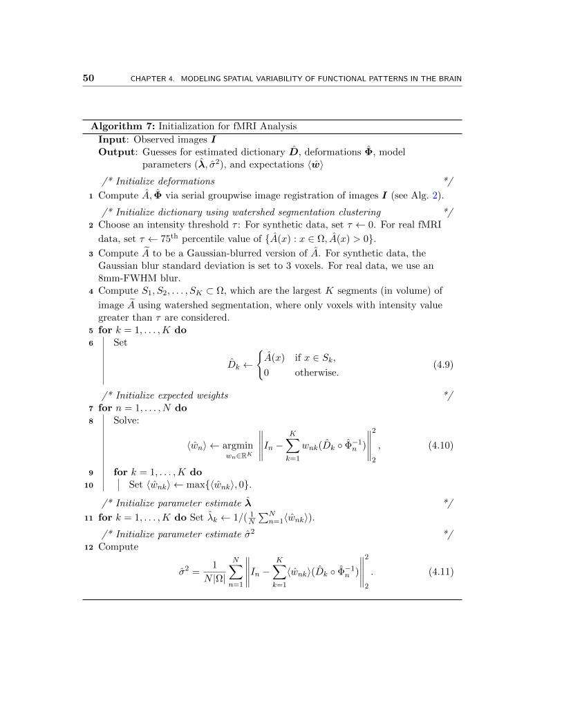
50 CHAPTER 4. MODELING SPATIAL VARIABILITY OF FUNCTIONAL PATTERNS IN THE BRAIN
Algorithm 7: Initialization for fMRI Analysis
Input: Observed images IOutput: Guesses for estimated dictionary D, deformations Φ, model
parameters (λ, σ2), and expectations 〈w〉/* Initialize deformations */
1 Compute A, Φ via serial groupwise image registration of images I (see Alg. 2).
/* Initialize dictionary using watershed segmentation clustering */2 Choose an intensity threshold τ : For synthetic data, set τ ← 0. For real fMRI
data, set τ ← 75th percentile value of A(x) : x ∈ Ω, A(x) > 0.3 Compute A to be a Gaussian-blurred version of A. For synthetic data, the
Gaussian blur standard deviation is set to 3 voxels. For real data, we use an8mm-FWHM blur.
4 Compute S1, S2, . . . , SK ⊂ Ω, which are the largest K segments (in volume) of
image A using watershed segmentation, where only voxels with intensity valuegreater than τ are considered.
5 for k = 1, . . . ,K do6 Set
Dk ←
A(x) if x ∈ Sk,0 otherwise.
(4.9)
/* Initialize expected weights */7 for n = 1, . . . , N do8 Solve:
〈wn〉 ← argminwn∈RK
∥∥∥∥∥In −K∑k=1
wnk(Dk Φ−1n )
∥∥∥∥∥2
2
, (4.10)
9 for k = 1, . . . ,K do10 Set 〈wnk〉 ← max〈wnk〉, 0.
/* Initialize parameter estimate λ */
11 for k = 1, . . . ,K do Set λk ← 1/( 1N
∑Nn=1〈wnk〉).
/* Initialize parameter estimate σ2 */12 Compute
σ2 =1
N |Ω|
N∑n=1
∥∥∥∥∥In −K∑k=1
〈wnk〉(Dk Φ−1n )
∥∥∥∥∥2
2
. (4.11)
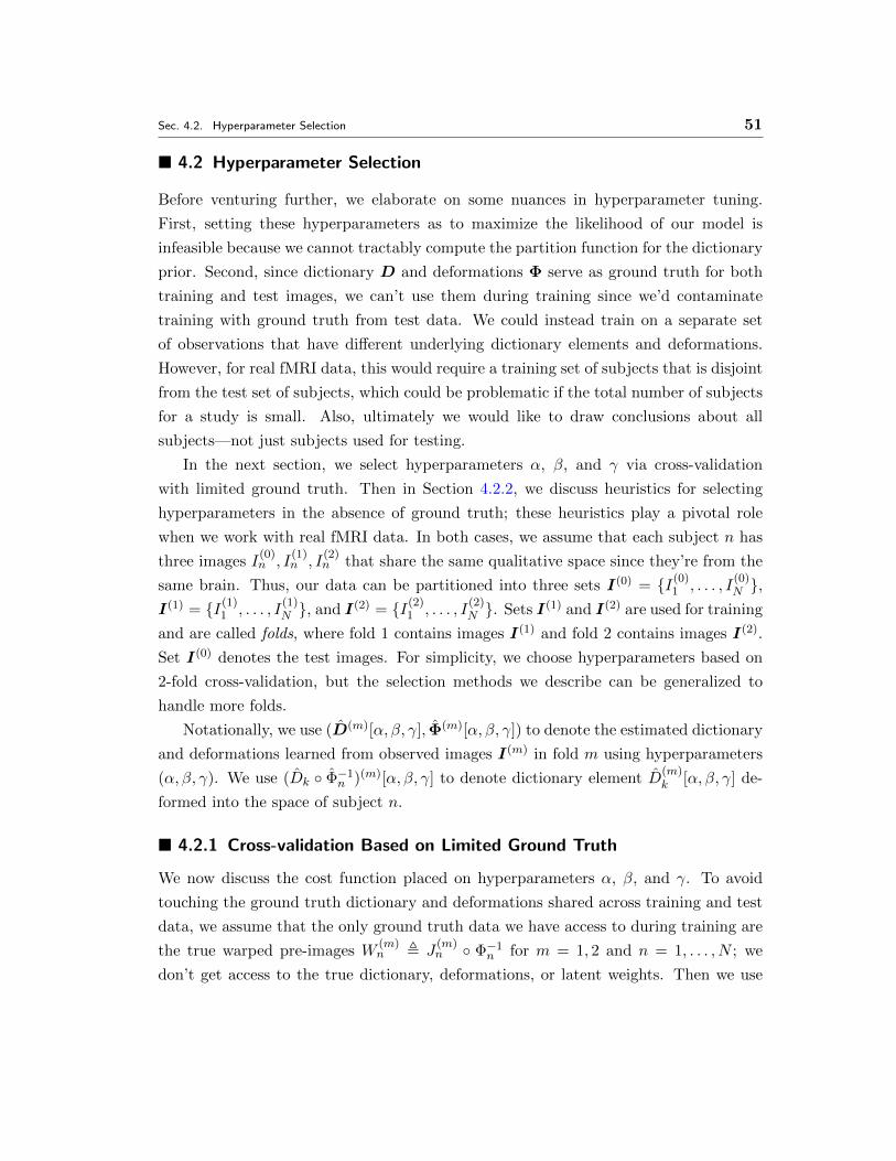
Sec. 4.2. Hyperparameter Selection 51
4.2 Hyperparameter Selection
Before venturing further, we elaborate on some nuances in hyperparameter tuning.
First, setting these hyperparameters as to maximize the likelihood of our model is
infeasible because we cannot tractably compute the partition function for the dictionary
prior. Second, since dictionary D and deformations Φ serve as ground truth for both
training and test images, we can’t use them during training since we’d contaminate
training with ground truth from test data. We could instead train on a separate set
of observations that have different underlying dictionary elements and deformations.
However, for real fMRI data, this would require a training set of subjects that is disjoint
from the test set of subjects, which could be problematic if the total number of subjects
for a study is small. Also, ultimately we would like to draw conclusions about all
subjects—not just subjects used for testing.
In the next section, we select hyperparameters α, β, and γ via cross-validation
with limited ground truth. Then in Section 4.2.2, we discuss heuristics for selecting
hyperparameters in the absence of ground truth; these heuristics play a pivotal role
when we work with real fMRI data. In both cases, we assume that each subject n has
three images I(0)n , I
(1)n , I
(2)n that share the same qualitative space since they’re from the
same brain. Thus, our data can be partitioned into three sets I(0) = I(0)1 , . . . , I
(0)N ,
I(1) = I(1)1 , . . . , I
(1)N , and I(2) = I(2)
1 , . . . , I(2)N . Sets I(1) and I(2) are used for training
and are called folds, where fold 1 contains images I(1) and fold 2 contains images I(2).
Set I(0) denotes the test images. For simplicity, we choose hyperparameters based on
2-fold cross-validation, but the selection methods we describe can be generalized to
handle more folds.
Notationally, we use (D(m)[α, β, γ], Φ(m)[α, β, γ]) to denote the estimated dictionary
and deformations learned from observed images I(m) in fold m using hyperparameters
(α, β, γ). We use (Dk Φ−1n )(m)[α, β, γ] to denote dictionary element D
(m)k [α, β, γ] de-
formed into the space of subject n.
4.2.1 Cross-validation Based on Limited Ground Truth
We now discuss the cost function placed on hyperparameters α, β, and γ. To avoid
touching the ground truth dictionary and deformations shared across training and test
data, we assume that the only ground truth data we have access to during training are
the true warped pre-images W(m)n , J
(m)n Φ−1
n for m = 1, 2 and n = 1, . . . , N ; we
don’t get access to the true dictionary, deformations, or latent weights. Then we use
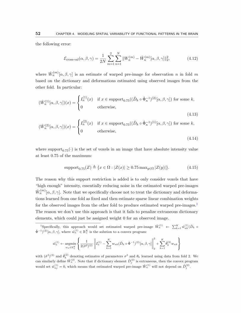
52 CHAPTER 4. MODELING SPATIAL VARIABILITY OF FUNCTIONAL PATTERNS IN THE BRAIN
the following error:
Ecross-val(α, β, γ) =1
2N
2∑m=1
N∑n=1
‖W (m)n − W (m)
n [α, β, γ]‖22, (4.12)
where W(m)n [α, β, γ] is an estimate of warped pre-image for observation n in fold m
based on the dictionary and deformations estimated using observed images from the
other fold. In particular:
(W (1)n [α, β, γ])(x) =
I(1)n (x) if x ∈ support0.75((Dk Φ−1
n )(2)[α, β, γ]) for some k,
0 otherwise,
(4.13)
(W (2)n [α, β, γ])(x) =
I(2)n (x) if x ∈ support0.75((Dk Φ−1
n )(1)[α, β, γ]) for some k,
0 otherwise,
(4.14)
where support0.75(·) is the set of voxels in an image that have absolute intensity value
at least 0.75 of the maximum:
support0.75(Z) , x ∈ Ω : |Z(x)| ≥ 0.75 maxy∈Ω |Z(y)|. (4.15)
The reason why this support restriction is added is to only consider voxels that have
“high enough” intensity, essentially reducing noise in the estimated warped pre-images
W(m)n [α, β, γ]. Note that we specifically choose not to treat the dictionary and deforma-
tions learned from one fold as fixed and then estimate sparse linear combination weights
for the observed images from the other fold to produce estimated warped pre-images.1
The reason we don’t use this approach is that it fails to penalize extraneous dictionary
elements, which could just be assigned weight 0 for an observed image.
1Specifically, this approach would set estimated warped pre-image W(1)n ←
∑Kk=1 w
(1)nk (Dk
Φ−1)(2)[α, β, γ], where w(1)n ∈ RK
+ is the solution to a convex program:
w(1)n ← argmin
wn∈RK+
1
2(σ2)(2)
∥∥∥∥∥I(1)n −
K∑k=1
wnk(Dk Φ−1)(2)[α, β, γ]
∥∥∥∥∥2
2
+K∑
k=1
θ(2)k wnk
with (σ2)(2) and θ
(2)k denoting estimates of parameters σ2 and θk learned using data from fold 2. We
can similarly define W(2)n . Note that if dictionary element D
(2)j is extraneous, then the convex program
would set w(1)nj = 0, which means that estimated warped pre-image W
(1)n will not depend on D
(2)j .

Sec. 4.2. Hyperparameter Selection 53
We choose hyperparameters (α, β, γ) as follows:
(α, β, γ) = argminα,β,γ∈0,102,104,106
Ecross-val(α, β, γ). (4.16)
Finally, we estimate dictionary D and deformations Φ using all observed training data
by training on images 12(I
(1)1 + I
(2)1 ), . . . , 1
2(I(1)N + I
(2)N ) with hyperparameters (α, β, γ).
The resulting training procedure is summarized in Alg. 8.
Algorithm 8: Training Using 2-Fold Cross-Validation with Limited Ground Truth
Input: Observed images IOutput: Estimated dictionary D, deformations Φ
1 Initialize Eoptcross-val ←∞, α← 0, β ← 0, γ ← 0.
2 for α, β, γ ∈ 0, 102, 104, 106 do
3 (Fold 1) Train on images I(1) = I(1)1 , . . . , I
(1)N using Alg. 6 with
hyperparameters (α, β, γ) to produce dictionary and deformation estimates(D(1)[α, β, γ], Φ(1)[α, β, γ]).
4 (Fold 2) Train on images I(2) = I(2)1 , . . . , I
(2)N using Alg. 6 with
hyperparameters (α, β, γ) to produce dictionary and deformation estimates(D(2)[α, β, γ], Φ(2)[α, β, γ]).
5 Using I, (D(1)[α, β, γ], Φ(1)[α, β, γ]), and (D(2)[α, β, γ], Φ(2)[α, β, γ]),compute Ecross-val(α, β, γ), given by eq. (4.12).
6 if Ecross-val(α, β, γ) < Eoptcross-val then
7 Set Eoptcross-val ← Ecross-val(α, β, γ), α← α, β ← β, γ ← γ.
8 Train on images I(1)1 +I
(2)1
2 , . . . ,I
(1)N +I
(2)N
2 using Alg. 6 with hyperparameters
(α, β, γ) to produce final dictionary and deformation estimates (D, Φ).
4.2.2 Heuristics in the Absence of Ground Truth
In the absence of ground truth, we use two key ideas to design heuristics for selecting
hyperparameters α, β, and γ while still taking advantage of training data comprising of
two separate folds. First, aligning observed images using estimated deformations should
boost peak values within each estimated dictionary element support, as suggested by
our toy example in Chapter 1. Second, by training separately on two different folds, the
estimated dictionaries and deformations should be consistent across the two folds. We
use two different consistency measures. In total, we have three heuristics, each giving
a score value in R that quantifies the quality of a choice of hyperparameters:
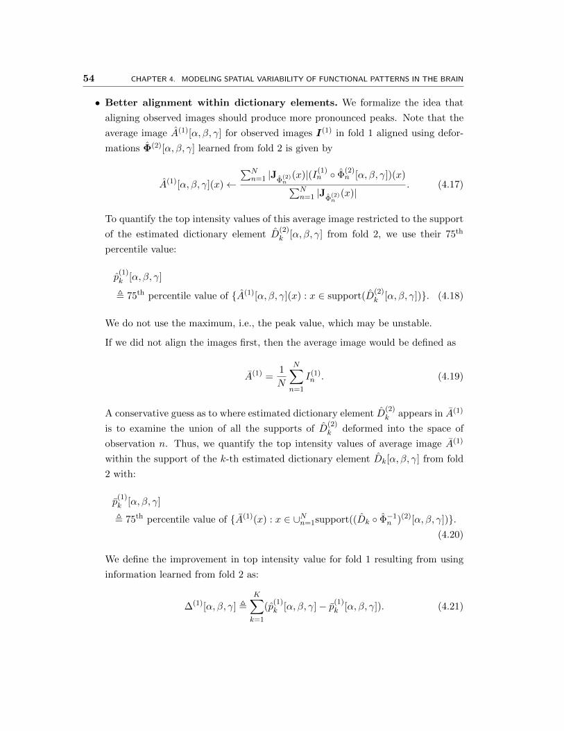
54 CHAPTER 4. MODELING SPATIAL VARIABILITY OF FUNCTIONAL PATTERNS IN THE BRAIN
• Better alignment within dictionary elements. We formalize the idea that
aligning observed images should produce more pronounced peaks. Note that the
average image A(1)[α, β, γ] for observed images I(1) in fold 1 aligned using defor-
mations Φ(2)[α, β, γ] learned from fold 2 is given by
A(1)[α, β, γ](x)←
∑Nn=1 |JΦ
(2)n
(x)|(I(1)n Φ
(2)n [α, β, γ])(x)∑N
n=1 |JΦ(2)n
(x)|. (4.17)
To quantify the top intensity values of this average image restricted to the support
of the estimated dictionary element D(2)k [α, β, γ] from fold 2, we use their 75th
percentile value:
p(1)k [α, β, γ]
, 75th percentile value of A(1)[α, β, γ](x) : x ∈ support(D(2)k [α, β, γ]). (4.18)
We do not use the maximum, i.e., the peak value, which may be unstable.
If we did not align the images first, then the average image would be defined as
A(1) =1
N
N∑n=1
I(1)n . (4.19)
A conservative guess as to where estimated dictionary element D(2)k appears in A(1)
is to examine the union of all the supports of D(2)k deformed into the space of
observation n. Thus, we quantify the top intensity values of average image A(1)
within the support of the k-th estimated dictionary element Dk[α, β, γ] from fold
2 with:
p(1)k [α, β, γ]
, 75th percentile value of A(1)(x) : x ∈ ∪Nn=1support((Dk Φ−1n )(2)[α, β, γ]).
(4.20)
We define the improvement in top intensity value for fold 1 resulting from using
information learned from fold 2 as:
∆(1)[α, β, γ] ,K∑k=1
(p(1)k [α, β, γ]− p(1)
k [α, β, γ]). (4.21)
Sec. 4.2. Hyperparameter Selection 55
We can similarly define A(2), A(2), p(2)k , p
(2)k , and ∆(2). The average intensity im-
provement score across folds is thus given by
Hintensity-improvement(α, β, γ) =1
2(∆(1)[α, β, γ] + ∆(2)[α, β, γ]), (4.22)
where higher is better.
• Consistency of alignment improvement across folds. We seek to avoid large
differences in improvement between the folds, suggesting a simple consistency
score:
Hintensity-improvement-difference(α, β, γ) = |∆(1)[α, β, γ]−∆(2)[α, β, γ]|, (4.23)
where lower is better.
• Consistency of dictionary element supports across folds. We want the
support of dictionary elements across folds to be similar. As the dictionary element
support across folds has different qualitative spaces, we compare the support across
folds instead in the qualitative space of the observations. To achieve this, we
measure the overlap between set Ω(1)n [α, β, γ] , ∪Kk=1support((DkΦ−1
n )(1)[α, β, γ])
and set Ω(2)n [α, β, γ] , ∪Kk=1support((Dk Φ−1
n )(2)[α, β, γ]) using the Dice volume
overlap measure [9]:
Dice(Ω(1)n [α, β, γ], Ω(2)
n [α, β, γ]) =2|Ω(1)
n [α, β, γ] ∩ Ω(2)n [α, β, γ]|
|Ω(1)n [α, β, γ]|+ |Ω(2)
n [α, β, γ]|, (4.24)
which only measures overlap in observation n’s qualitative space. Averaging across
all observations’ qualitative spaces gives the consistency score
Hdictionary-consistency(α, β, γ) =1
N
N∑n=1
Dice(Ω(1)n [α, β, γ], Ω(2)
n [α, β, γ]), (4.25)
which is a value between 0 (no overlap) and 1 (perfect overlap); higher is better.
To select which hyperparameter setting to use, we handpick a hyperparameter setting
that provides a good trade-off between all three heuristics.
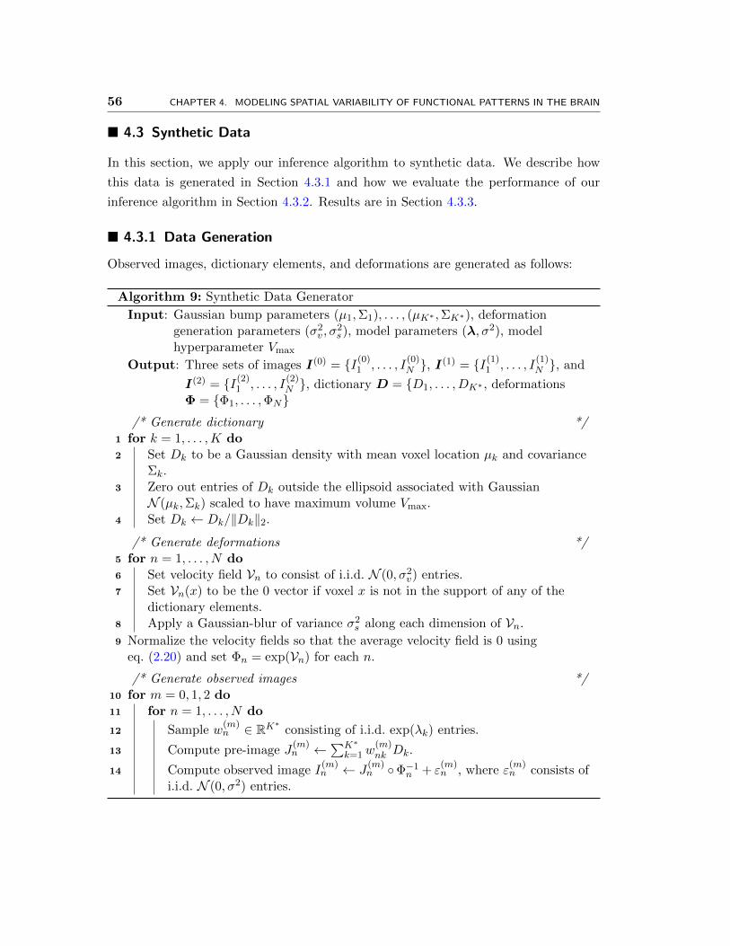
56 CHAPTER 4. MODELING SPATIAL VARIABILITY OF FUNCTIONAL PATTERNS IN THE BRAIN
4.3 Synthetic Data
In this section, we apply our inference algorithm to synthetic data. We describe how
this data is generated in Section 4.3.1 and how we evaluate the performance of our
inference algorithm in Section 4.3.2. Results are in Section 4.3.3.
4.3.1 Data Generation
Observed images, dictionary elements, and deformations are generated as follows:
Algorithm 9: Synthetic Data Generator
Input: Gaussian bump parameters (µ1,Σ1), . . . , (µK∗ ,ΣK∗), deformationgeneration parameters (σ2
v , σ2s), model parameters (λ, σ2), model
hyperparameter Vmax
Output: Three sets of images I(0) = I(0)1 , . . . , I
(0)N , I(1) = I(1)
1 , . . . , I(1)N , and
I(2) = I(2)1 , . . . , I
(2)N , dictionary D = D1, . . . , DK∗ , deformations
Φ = Φ1, . . . ,ΦN/* Generate dictionary */
1 for k = 1, . . . ,K do2 Set Dk to be a Gaussian density with mean voxel location µk and covariance
Σk.3 Zero out entries of Dk outside the ellipsoid associated with Gaussian
N (µk,Σk) scaled to have maximum volume Vmax.4 Set Dk ← Dk/‖Dk‖2.
/* Generate deformations */5 for n = 1, . . . , N do6 Set velocity field Vn to consist of i.i.d. N (0, σ2
v) entries.7 Set Vn(x) to be the 0 vector if voxel x is not in the support of any of the
dictionary elements.8 Apply a Gaussian-blur of variance σ2
s along each dimension of Vn.
9 Normalize the velocity fields so that the average velocity field is 0 usingeq. (2.20) and set Φn = exp(Vn) for each n.
/* Generate observed images */10 for m = 0, 1, 2 do11 for n = 1, . . . , N do
12 Sample w(m)n ∈ RK∗ consisting of i.i.d. exp(λk) entries.
13 Compute pre-image J(m)n ←
∑K∗
k=1w(m)nk Dk.
14 Compute observed image I(m)n ← J
(m)n Φ−1
n + ε(m)n , where ε
(m)n consists of
i.i.d. N (0, σ2) entries.
Sec. 4.3. Synthetic Data 57
We specifically generate 100-by-100 images with the above procedure using parame-
ters µ1 = (45, 35), µ2 = (40, 60), µ3 = (65, 55), µ4 = (60, 40), Σ1 = 2I, Σ2 = I, Σ3 = 3I,
Σ4 = 4I, λ = (1/5, 1/8, 1/4, 1/10), V ∗max = 300, σ2v = 4000, σ2
s = 36, and σ2 = 1. Speci-
fying a maximum ellipse semi-axis length r∗max is unnecessary as our generative process
implies the existence of some r∗max. The dictionary generated is shown in Fig. 4.1a.
Examples of the generated pre-images with their corresponding observed images are
shown in Fig. 4.2. For the specific values of the parameters for σ2v and σ2
s we use to
generate these images, we find that our volume change condition is met with φmax = 4.
For inference, we set the number of estimated dictionary elements to K = 10, the
maximum ellipse volume to Vmax = 500 voxels3, and the maximum ellipse semi-axis
length to rmax = 10 voxels. With these parameters treated as fixed, we only need to
tune hyperparameters α, β, and γ.
4.3.2 Evaluation
To assess error in test data, we use several error measures:
• Deformation error. We use error
Edeformations(Φ; Φ) =1
N
N∑n=1
∑x∈Ω
‖Φn(x)− Φn(x)‖22. (4.26)
• Dictionary error. Since the number of true dictionary elements K∗ and the
number of estimated dictionary elements K are, in general, not equal, we need to
compute a matching between the dictionaries. For simplicity, we consider the case
when K∗ < K. Then the error we use is
Edictionary(D;D) = minρ∈SK
K∗∑k=1
‖Dρ(k) −Dk‖22 +
K∑k=K∗+1
‖Dρ(k)‖22
, (4.27)
where SK is the set of all permutations of 1, . . . ,K.
Note that for ρ ∈ SK , we can actually reorder ρ(K∗+1), . . . , ρ(K) and the objective
function would be unaffected, so we’re actually only optimizing over K!/(K−K∗)!assignments, namely the subset of estimated dictionary elements that map to the
true dictionary elements under ρ.
• Group average error. This error measures how far an estimate of the average
group signal is from the true group average signal that perfectly accounts for
58 CHAPTER 4. MODELING SPATIAL VARIABILITY OF FUNCTIONAL PATTERNS IN THE BRAIN
misalignment. Formally, for test images I(0) = I(0)1 , . . . , I
(0)N with pre-images
J (0) = J (0)1 , . . . , J
(0)N , the true group average image is
A(0) =1
N
N∑n=1
J (0)n , (4.28)
which can also be interpreted as the true group average response had we known
all the deformations for aligning the images and had there been no noise.
We estimate pre-images for the test images using our dictionary and deformation
estimates:
J (0)n (x) =
(I(0)n Φn)(x) if x is in the spatial support of Dk for some k,
0 otherwise.
(4.29)
Averaging these pre-image estimates creates
A(0) ← 1
N
N∑n=1
J (0)n . (4.30)
Unfortunately, images A(0) and A(0) do not share the same qualitative space since
the former has qualitative space defined by the true dictionary while the latter
has one defined by the estimated dictionary. Thus, we can’t compare images A(0)
and A(0) directly. However, we can bring both images A(0) and A(0) into the qual-
itative space of observation n before computing the squared `2 distance between
them, i.e., ‖A(0) Φ−1n − A(0) Φ−1
n ‖22. Repeating this distance calculation in the
qualitative space of all observations n = 1, . . . , N and averaging produces the final
group average error:
Egroup-average(D, Φ; I(0),J (0),Φ) =1
N
N∑n=1
‖A(0) Φ−1n −A(0) Φ−1
n ‖22, (4.31)
where A(0) depends on I(0), D, and Φ while A(0) depends on J (0).
4.3.3 Results
We compare our results from cross-validation training of our inference algorithm (la-
beled deformation-invariant sparse coding in tables and plots) against the baseline of
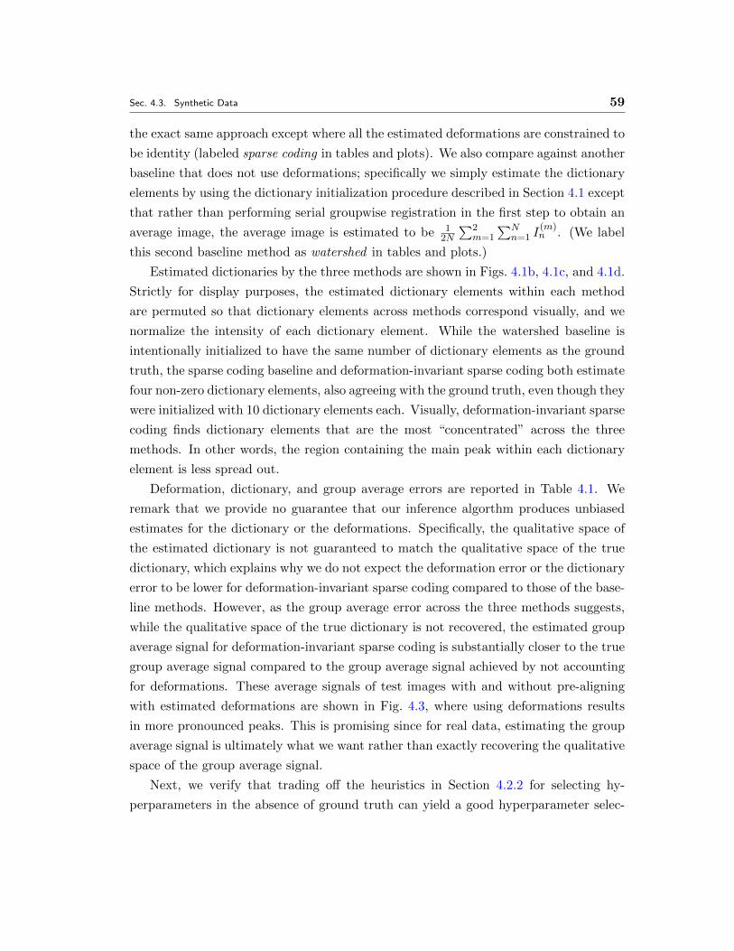
Sec. 4.3. Synthetic Data 59
the exact same approach except where all the estimated deformations are constrained to
be identity (labeled sparse coding in tables and plots). We also compare against another
baseline that does not use deformations; specifically we simply estimate the dictionary
elements by using the dictionary initialization procedure described in Section 4.1 except
that rather than performing serial groupwise registration in the first step to obtain an
average image, the average image is estimated to be 12N
∑2m=1
∑Nn=1 I
(m)n . (We label
this second baseline method as watershed in tables and plots.)
Estimated dictionaries by the three methods are shown in Figs. 4.1b, 4.1c, and 4.1d.
Strictly for display purposes, the estimated dictionary elements within each method
are permuted so that dictionary elements across methods correspond visually, and we
normalize the intensity of each dictionary element. While the watershed baseline is
intentionally initialized to have the same number of dictionary elements as the ground
truth, the sparse coding baseline and deformation-invariant sparse coding both estimate
four non-zero dictionary elements, also agreeing with the ground truth, even though they
were initialized with 10 dictionary elements each. Visually, deformation-invariant sparse
coding finds dictionary elements that are the most “concentrated” across the three
methods. In other words, the region containing the main peak within each dictionary
element is less spread out.
Deformation, dictionary, and group average errors are reported in Table 4.1. We
remark that we provide no guarantee that our inference algorthm produces unbiased
estimates for the dictionary or the deformations. Specifically, the qualitative space of
the estimated dictionary is not guaranteed to match the qualitative space of the true
dictionary, which explains why we do not expect the deformation error or the dictionary
error to be lower for deformation-invariant sparse coding compared to those of the base-
line methods. However, as the group average error across the three methods suggests,
while the qualitative space of the true dictionary is not recovered, the estimated group
average signal for deformation-invariant sparse coding is substantially closer to the true
group average signal compared to the group average signal achieved by not accounting
for deformations. These average signals of test images with and without pre-aligning
with estimated deformations are shown in Fig. 4.3, where using deformations results
in more pronounced peaks. This is promising since for real data, estimating the group
average signal is ultimately what we want rather than exactly recovering the qualitative
space of the group average signal.
Next, we verify that trading off the heuristics in Section 4.2.2 for selecting hy-
perparameters in the absence of ground truth can yield a good hyperparameter selec-
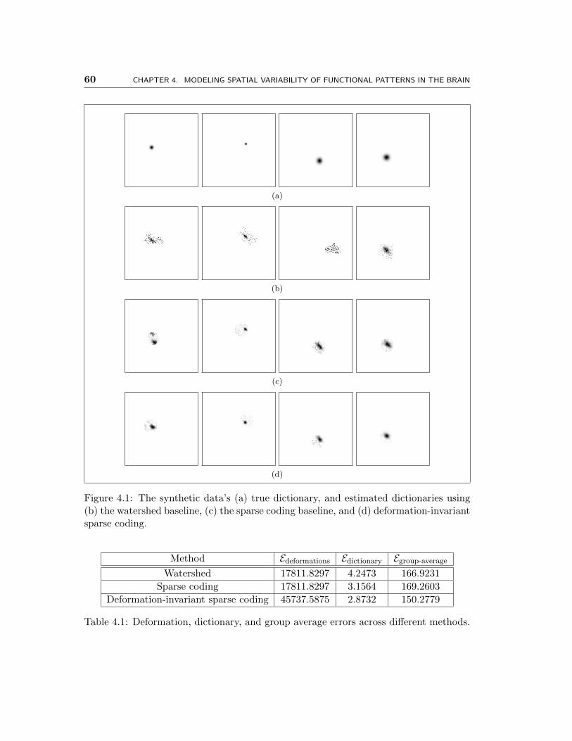
60 CHAPTER 4. MODELING SPATIAL VARIABILITY OF FUNCTIONAL PATTERNS IN THE BRAIN
(a)
(b)
(c)
(d)
Figure 4.1: The synthetic data’s (a) true dictionary, and estimated dictionaries using(b) the watershed baseline, (c) the sparse coding baseline, and (d) deformation-invariantsparse coding.
Method Edeformations Edictionary Egroup-average
Watershed 17811.8297 4.2473 166.9231
Sparse coding 17811.8297 3.1564 169.2603
Deformation-invariant sparse coding 45737.5875 2.8732 150.2779
Table 4.1: Deformation, dictionary, and group average errors across different methods.
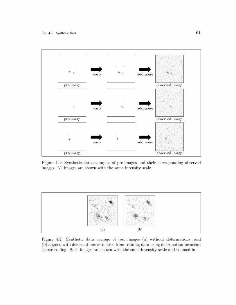
Sec. 4.3. Synthetic Data 61
warp add noise
pre-image observed image
warp add noise
pre-image observed image
warp add noise
pre-image observed image
Figure 4.2: Synthetic data examples of pre-images and their corresponding observedimages. All images are shown with the same intensity scale.
(a) (b)
Figure 4.3: Synthetic data average of test images (a) without deformations, and(b) aligned with deformations estimated from training data using deformation-invariantsparse coding. Both images are shown with the same intensity scale and zoomed in.
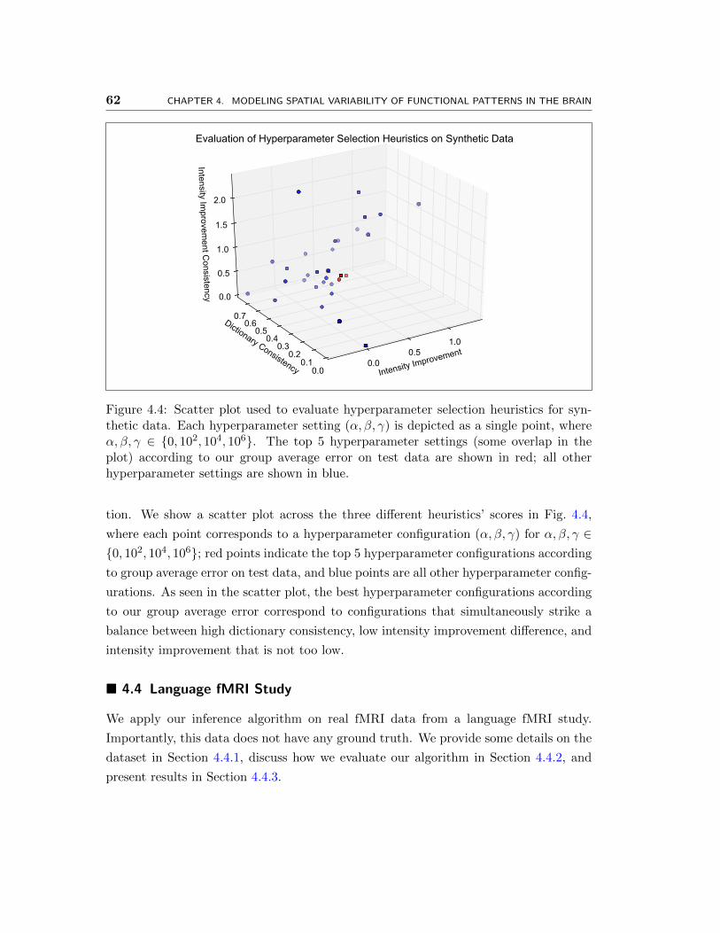
62 CHAPTER 4. MODELING SPATIAL VARIABILITY OF FUNCTIONAL PATTERNS IN THE BRAIN
Intensity Improvement0.0
0.51.0
Dictionary Consistency 0.00.1
0.20.3
0.40.5
0.60.7
Intensity Improvem
ent Consistency 0.0
0.5
1.0
1.5
2.0
Evaluation of Hyperparameter Selection Heuristics on Synthetic Data
Figure 4.4: Scatter plot used to evaluate hyperparameter selection heuristics for syn-thetic data. Each hyperparameter setting (α, β, γ) is depicted as a single point, whereα, β, γ ∈ 0, 102, 104, 106. The top 5 hyperparameter settings (some overlap in theplot) according to our group average error on test data are shown in red; all otherhyperparameter settings are shown in blue.
tion. We show a scatter plot across the three different heuristics’ scores in Fig. 4.4,
where each point corresponds to a hyperparameter configuration (α, β, γ) for α, β, γ ∈0, 102, 104, 106; red points indicate the top 5 hyperparameter configurations according
to group average error on test data, and blue points are all other hyperparameter config-
urations. As seen in the scatter plot, the best hyperparameter configurations according
to our group average error correspond to configurations that simultaneously strike a
balance between high dictionary consistency, low intensity improvement difference, and
intensity improvement that is not too low.
4.4 Language fMRI Study
We apply our inference algorithm on real fMRI data from a language fMRI study.
Importantly, this data does not have any ground truth. We provide some details on the
dataset in Section 4.4.1, discuss how we evaluate our algorithm in Section 4.4.2, and
present results in Section 4.4.3.
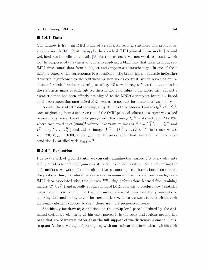
Sec. 4.4. Language fMRI Study 63
4.4.1 Data
Our dataset is from an fMRI study of 82 subjects reading sentences and pronounce-
able non-words [14]. First, we apply the standard fMRI general linear model [16] and
weighted random effects analysis [33] for the sentences vs. non-words contrast, which
for the purposes of this thesis amounts to applying a black box that takes as input raw
fMRI time course data from a subject and outputs a t-statistic map. In one of these
maps, a voxel, which corresponds to a location in the brain, has a t-statistic indicating
statistical significance to the sentences vs. non-words contrast, which serves as an in-
dicator for lexical and structural processing. Observed images I are thus taken to be
the t-statistic maps of each subject thresholded at p-value=0.01, where each subject’s
t-statistic map has been affinely pre-aligned to the MNI305 template brain [13] based
on the corresponding anatomical MRI scan as to account for anatomical variability.
As with the synthetic data setting, subject n has three observed images I(0)n , I
(1)n , I
(2)n ,
each originating from a separate run of the fMRI protocol where the subject was asked
to essentially repeat the same language task. Each image I(m)n is of size 128×128×128,
where each voxel is of (2mm)3 volume. We train on images I(1) = I(1)1 , . . . , I
(1)N and
I(2) = I(2)1 , . . . , I
(2)N and test on images I(0) = I(0)
1 , . . . , I(0)N . For inference, we set
K = 20, Vmax = 1000, and rmax = 7. Empirically, we find that the volume change
condition is satisfied with φmax = 2.
4.4.2 Evaluation
Due to the lack of ground truth, we can only examine the learned dictionary elements
and qualitatively compare against existing neuroscience literature. As for validating the
deformations, we work off the intuition that accounting for deformations should make
the peaks within group-level parcels more pronounced. To this end, we pre-align raw
fMRI data associated with test images I(0) using deformations learned from training
images (I(1), I(2)) and actually re-run standard fMRI analysis to produce new t-statistic
maps, which now account for the deformations learned; this essentially amounts to
applying deformation Φn to I(0)n for each subject n. Then we want to look within each
dictionary element support to see if there are more pronounced peaks.
Specifically for drawing conclusions on the group-level parcels defined by the esti-
mated dictionary elements, within each parcel, it is the peak and regions around the
peak that are of interest rather than the full support of the dictionary element. Thus,
to quantify the advantage of pre-aligning with our estimated deformations, within each
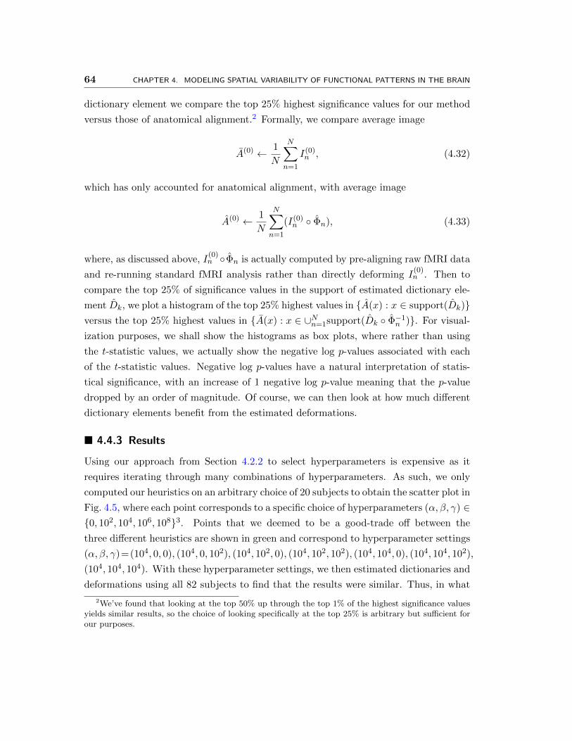
64 CHAPTER 4. MODELING SPATIAL VARIABILITY OF FUNCTIONAL PATTERNS IN THE BRAIN
dictionary element we compare the top 25% highest significance values for our method
versus those of anatomical alignment.2 Formally, we compare average image
A(0) ← 1
N
N∑n=1
I(0)n , (4.32)
which has only accounted for anatomical alignment, with average image
A(0) ← 1
N
N∑n=1
(I(0)n Φn), (4.33)
where, as discussed above, I(0)n Φn is actually computed by pre-aligning raw fMRI data
and re-running standard fMRI analysis rather than directly deforming I(0)n . Then to
compare the top 25% of significance values in the support of estimated dictionary ele-
ment Dk, we plot a histogram of the top 25% highest values in A(x) : x ∈ support(Dk)versus the top 25% highest values in A(x) : x ∈ ∪Nn=1support(Dk Φ−1
n ). For visual-
ization purposes, we shall show the histograms as box plots, where rather than using
the t-statistic values, we actually show the negative log p-values associated with each
of the t-statistic values. Negative log p-values have a natural interpretation of statis-
tical significance, with an increase of 1 negative log p-value meaning that the p-value
dropped by an order of magnitude. Of course, we can then look at how much different
dictionary elements benefit from the estimated deformations.
4.4.3 Results
Using our approach from Section 4.2.2 to select hyperparameters is expensive as it
requires iterating through many combinations of hyperparameters. As such, we only
computed our heuristics on an arbitrary choice of 20 subjects to obtain the scatter plot in
Fig. 4.5, where each point corresponds to a specific choice of hyperparameters (α, β, γ) ∈0, 102, 104, 106, 1083. Points that we deemed to be a good-trade off between the
three different heuristics are shown in green and correspond to hyperparameter settings
(α, β, γ)=(104, 0, 0), (104, 0, 102), (104, 102, 0), (104, 102, 102), (104, 104, 0), (104, 104, 102),
(104, 104, 104). With these hyperparameter settings, we then estimated dictionaries and
deformations using all 82 subjects to find that the results were similar. Thus, in what
2We’ve found that looking at the top 50% up through the top 1% of the highest significance valuesyields similar results, so the choice of looking specifically at the top 25% is arbitrary but sufficient forour purposes.
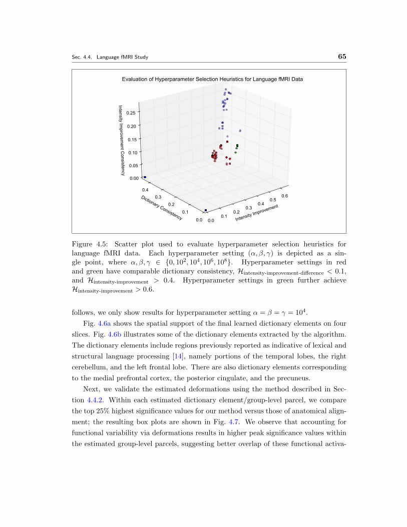
Sec. 4.4. Language fMRI Study 65
Intensity Improvement
0.00.1
0.20.3
0.40.5
0.6Dictionary Consistency 0.0
0.10.2
0.30.4
Intensity Improvem
ent Consistency
0.00
0.05
0.10
0.15
0.20
0.25
Evaluation of Hyperparameter Selection Heuristics for Language fMRI Data
Figure 4.5: Scatter plot used to evaluate hyperparameter selection heuristics forlanguage fMRI data. Each hyperparameter setting (α, β, γ) is depicted as a sin-gle point, where α, β, γ ∈ 0, 102, 104, 106, 108. Hyperparameter settings in redand green have comparable dictionary consistency, Hintensity-improvement-difference < 0.1,and Hintensity-improvement > 0.4. Hyperparameter settings in green further achieveHintensity-improvement > 0.6.
follows, we only show results for hyperparameter setting α = β = γ = 104.
Fig. 4.6a shows the spatial support of the final learned dictionary elements on four
slices. Fig. 4.6b illustrates some of the dictionary elements extracted by the algorithm.
The dictionary elements include regions previously reported as indicative of lexical and
structural language processing [14], namely portions of the temporal lobes, the right
cerebellum, and the left frontal lobe. There are also dictionary elements corresponding
to the medial prefrontal cortex, the posterior cingulate, and the precuneus.
Next, we validate the estimated deformations using the method described in Sec-
tion 4.4.2. Within each estimated dictionary element/group-level parcel, we compare
the top 25% highest significance values for our method versus those of anatomical align-
ment; the resulting box plots are shown in Fig. 4.7. We observe that accounting for
functional variability via deformations results in higher peak significance values within
the estimated group-level parcels, suggesting better overlap of these functional activa-

66 CHAPTER 4. MODELING SPATIAL VARIABILITY OF FUNCTIONAL PATTERNS IN THE BRAIN
(a)
(b)
Figure 4.6: Estimated dictionary. (a) Four slices of a map showing the spatial supportof the extracted dictionary elements. Different colors correspond to distinct dictionaryelements where there is some overlap between dictionary elements. From left to right:left frontal lobe and temporal regions, medial prefrontal cortex and posterior cingu-late/precuneus, right cerebellum, and right temporal lobe. Dictionary element indicescorrespond to those in Fig. 4.7. (b) A single slice from three different estimated dictio-nary elements where relative intensity varies from high (red) to low (blue). From leftto right: left posterior temporal lobe, left anterior temporal lobe, left inferior frontalgyrus.
00 A
F
01 A
F
02 A
F
03 A
F
04 A
F
05 A
F
06 A
F
07 A
F
08 A
F
09 A
F
10 A
F
11 A
F
12 A
F
13 A
F
14 A
F
15 A
F
16 A
F
17 A
F
18 A
F
19 A
F
Dictionary element index
0
5
10
15
20
−lo
g 10(p)
Weighted Random Effects Group Analysis
Anatomical alignment
Functional alignment (our model)
Figure 4.7: Box plots of top 25% weighted random effects analysis significance valueswithin dictionary element supports. For each dictionary element, “A” refers to anatom-ical alignment, and “F” refers to alignment via deformations learned by our model.
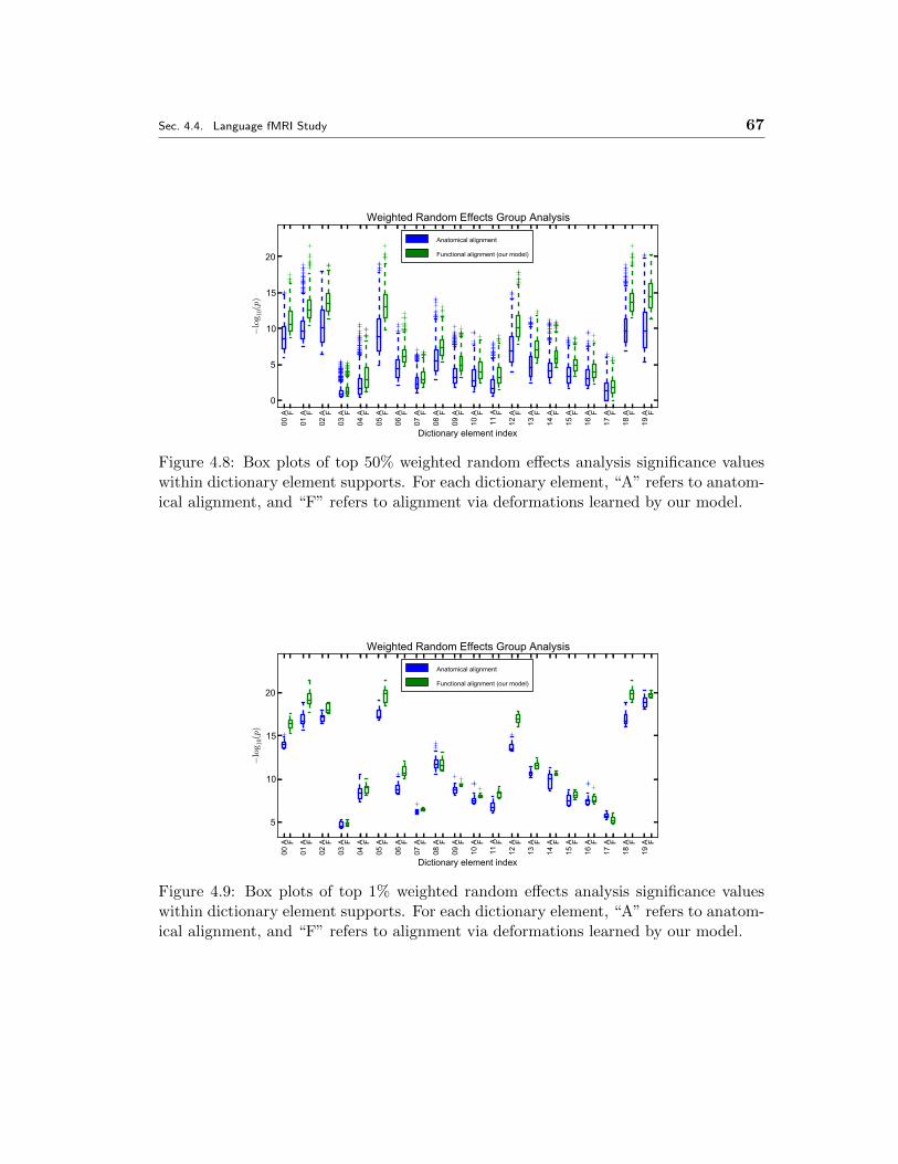
Sec. 4.4. Language fMRI Study 67
00 A
F
01 A
F
02 A
F
03 A
F
04 A
F
05 A
F
06 A
F
07 A
F
08 A
F
09 A
F
10 A
F
11 A
F
12 A
F
13 A
F
14 A
F
15 A
F
16 A
F
17 A
F
18 A
F
19 A
F
Dictionary element index
0
5
10
15
20−
log 1
0(p
)
Weighted Random Effects Group Analysis
Anatomical alignment
Functional alignment (our model)
Figure 4.8: Box plots of top 50% weighted random effects analysis significance valueswithin dictionary element supports. For each dictionary element, “A” refers to anatom-ical alignment, and “F” refers to alignment via deformations learned by our model.
00 A
F
01 A
F
02 A
F
03 A
F
04 A
F
05 A
F
06 A
F
07 A
F
08 A
F
09 A
F
10 A
F
11 A
F
12 A
F
13 A
F
14 A
F
15 A
F
16 A
F
17 A
F
18 A
F
19 A
F
Dictionary element index
5
10
15
20
−lo
g 10(p
)
Weighted Random Effects Group Analysis
Anatomical alignment
Functional alignment (our model)
Figure 4.9: Box plots of top 1% weighted random effects analysis significance valueswithin dictionary element supports. For each dictionary element, “A” refers to anatom-ical alignment, and “F” refers to alignment via deformations learned by our model.
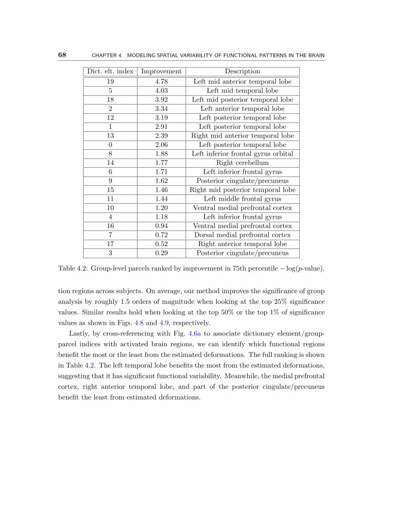
68 CHAPTER 4. MODELING SPATIAL VARIABILITY OF FUNCTIONAL PATTERNS IN THE BRAIN
Dict. elt. index Improvement Description
19 4.78 Left mid anterior temporal lobe
5 4.03 Left mid temporal lobe
18 3.92 Left mid posterior temporal lobe
2 3.34 Left anterior temporal lobe
12 3.19 Left posterior temporal lobe
1 2.91 Left posterior temporal lobe
13 2.39 Right mid anterior temporal lobe
0 2.06 Left posterior temporal lobe
8 1.88 Left inferior frontal gyrus orbital
14 1.77 Right cerebellum
6 1.71 Left inferior frontal gyrus
9 1.62 Posterior cingulate/precuneus
15 1.46 Right mid posterior temporal lobe
11 1.44 Left middle frontal gyrus
10 1.20 Ventral medial prefrontal cortex
4 1.18 Left inferior frontal gyrus
16 0.94 Ventral medial prefrontal cortex
7 0.72 Dorsal medial prefrontal cortex
17 0.52 Right anterior temporal lobe
3 0.29 Posterior cingulate/precuneus
Table 4.2: Group-level parcels ranked by improvement in 75th percentile − log(p-value).
tion regions across subjects. On average, our method improves the significance of group
analysis by roughly 1.5 orders of magnitude when looking at the top 25% significance
values. Similar results hold when looking at the top 50% or the top 1% of significance
values as shown in Figs. 4.8 and 4.9, respectively.
Lastly, by cross-referencing with Fig. 4.6a to associate dictionary element/group-
parcel indices with activated brain regions, we can identify which functional regions
benefit the most or the least from the estimated deformations. The full ranking is shown
in Table 4.2. The left temporal lobe benefits the most from the estimated deformations,
suggesting that it has significant functional variability. Meanwhile, the medial prefrontal
cortex, right anterior temporal lobe, and part of the posterior cingulate/precuneus
benefit the least from estimated deformations.
Chapter 5
Discussion and Conclusions
This thesis has extended sparse coding to account for deformations and provided an ac-
companying inference algorithm that can take advantage of existing work in image reg-
istration. Our treatment has largely been algorithmic rather than theoretical. Natural
questions that arise are how inference can be changed to provide theoretical guarantees
for consistently estimating dictionary and deformations, and how much observed data
is needed to obtain accurate dictionary and deformation estimates. The latter question
has practical implications as to determine how many subjects are needed for an fMRI
study if deformation-invariant sparse coding is to be used. The former question remains
open; Kurtek et al. [20] have recently resolved the case of a single dictionary element
and noise that is a single unknown constant across observations, but analyzing our more
general setting has yet to be done.
On the neuroscience side, more validation is needed to justify the usefulness of
modeling functional variability using deformation-invariant sparse coding. A direction
worth exploring is to see whether an estimated dictionary learned from, say, a language
study can be used as markers for a new study with a different stimulus to see how
the new stimulus relates to language processing. If the estimated dictionary indeed
provides a more accurate assessment of the stimulus used to train the dictionary than
other existing approaches, then we could confirm the utility of our model and hopefully
use it for neuroscientific discovery.
69

70 CHAPTER 5. DISCUSSION AND CONCLUSIONS
Appendix A
Deriving the Inference Algorithm
We derive our EM-like inference algorithm in Chapter 3. Specifically, we would like to
solve optimization problem (3.2), which is equivalent to solving
(D, Φ, λ, σ2)← argminD,Φ,λ,σ2
∫p(I,w,Φ,D;λ, σ2)dw. (A.1)
The full joint distribution in the integrand is given by eq. (3.6), reproduced below for
convenience:
p(I,w,Φ,D;λ, σ2)
∝N∏n=1
pΦ(Φn)
K∏k=1
pw(wnk;λk)∏x∈Ω
N
(In(x);
K∑k=1
wnkDk(Φ−1n (x)), σ2
)
· exp
−K∑k=1
(α‖Dk‖1 +β
2D>k LDk)− γ
∑k 6=`‖Dk D`‖1
, (A.2)
where average deformation Φ1 · · · Φn is identity; each Dk satisfies ‖Dk‖2 ≤ 1 and has
spatial support contained within an ellipsoid of volume Vmax and maximum semi-axis
length rmax; and hyperparameters α, β, γ, Vmax, and rmax are treated as constants.
Distributions pw(·;λk) and pΦ(·) are left general. We specialize to the case of exponen-
tial pw and positive normal qw in Appendix B, which builds off the results of this section.
Importantly, our derivations in this section work with any registration framework that
minimizes an energy of the form in eq. (3.3).
Since marginalizing out the latent weights w in optimization problem (A.1) is in-
tractable, the EM algorithm instead locally maximizes a lower bound on log likelihood
log p(I,Φ,D;λ, σ2). In particular, using Jensen’s inequality and introducing an auxil-
71
72 APPENDIX A. DERIVING THE INFERENCE ALGORITHM
iary distribution q(w) over latent weights w, we have
log p(I,Φ,D;λ, σ2) = log
∫q(w|I,Φ,D;λ, σ2)
p(I,w,Φ,D;λ, σ2)
q(w|I,Φ,D;λ, σ2)dw
= logEq[p(I,w,Φ,D;λ, σ2)
q(w|I,Φ,D;λ, σ2)
∣∣∣∣ I,Φ,D]≥ Eq
[log
p(I,w,Φ,D;λ, σ2)
q(w|I,Φ,D;λ, σ2)
∣∣∣∣ I,Φ,D]=
N∑n=1
[log pΦ(Φn) +
K∑k=1
Eq[log pw(wnk;λk)|I,Φ,D]
− 1
2σ2Eq
∥∥∥∥∥In −K∑k=1
wnk(Dk Φ−1n )
∥∥∥∥∥2
2
∣∣∣∣∣∣ I,Φ,D
− N |Ω|2
log(2πσ2) +H(q) + log p(D) + constant
, L(q,Φ,D,λ, σ2), (A.3)
where H(q) is the differential entropy of distribution q(w). The EM algorithm itera-
tively maximizes this lower bound L(q,Φ,D,λ, σ2) via coordinate ascent until reaching
a local maximum. Exact EM calls for choosing q(w) = p(w|I,Φ,D;λ, σ2); however,
with this choice of q and by inspecting the graphical model (Fig. 3.2), once we condition
on observed images I, all the weights wnk for the same n become coupled, rendering ex-
pectation Eq[‖In −∑K
k=1wnk(Dk Φ−1n )‖22|I,Φ,D] intractable to compute due to the
marginalizations required. Thus, we choose auxiliary distribution q to be a variational
approximation to the distribution p(w|I,Φ,D;λ, σ2) where q has factorization
q(w;ψ) =
N∏n=1
K∏k=1
qw(wnk;ψnk), (A.4)
and distribution qw(·;ψnk) is parameterized by ψnk. With this choice of q and a bit of
73
algebra, lower bound L in inequality (A.3) can be written as
L(q(·;ψ),Φ,D,λ, σ2)
=
N∑n=1
[log pΦ(Φn) +
K∑k=1
Eqw [log pw(wnk;λk)|I,Φ,D]
− 1
2σ2
∥∥∥∥∥In −K∑k=1
〈wnk〉(Dk Φ−1n )
∥∥∥∥∥2
2
+K∑k=1
(〈w2nk〉 − 〈wnk〉2)‖Dk Φ−1
n ‖22
− N |Ω|
2log(2πσ2) +
N∑n=1
K∑k=1
H(qw(·;ψnk)) + log p(D) + constant
, L−(ψ,Φ,D,λ, σ2), (A.5)
where 〈wnk〉 , Eq[wnk|I,Φ,D] and 〈w2nk〉 , Eq[w2
nk|I,Φ,D].
Since q is chosen to not necessarily be the optimal choice q(w) = p(w|I,Φ,D;λ, σ2),
the E-step of the resulting EM-like algorithm does not guarantee maximization of lower
bound L of ineq. (A.3) over all possible distributions for latent weights w but instead
maximizes the looser variational lower bound L−. This approximation results in a
variational EM algorithm [38]. For part of the M-step, we maximize an even looser
approximate lower bound on the log likelihood. Effectively, our inference algorithm
is based on the EM algorithm but lacks theoretical guarantees of the latter due to
approximations we make. Moreover, maximizing looser bounds does not guarantee an
increase in the log likelihood at each step, so our algorithm is not a generalized EM
algorithm.
Equipped with variational lower bound L−, we’re ready to derive the steps of each
iteration of our inference algorithm. First, we let (Φ, D, λ, σ2, ψ) be current estimates
for (Φ,D,λ, σ2,ψ) and denote 〈wnk〉 , Eqw [wnk|I, Φ, D], 〈w2nk〉 , Eqw [w2
nk|I, Φ, D],
and qw = qw(·; ψnk). Then our EM-like algorithm alternates between the following
steps:
E-step. Compute
ψ ← argmaxψ
L−(ψ, Φ, D, λ, σ2). (A.6)
Then compute expectations 〈wnk〉 and 〈w2nk〉 for all n and k.
74 APPENDIX A. DERIVING THE INFERENCE ALGORITHM
M-step. Compute
(Φ, D, λ, σ2)← argmaxΦ,D,λ,σ2
L−(ψ,Φ,D,λ, σ2), (A.7)
which depends on expectations 〈wnk〉 and 〈w2nk〉.
The next sections detail how each step is carried out.
A.1 E-step
Rather than simultaneously updating all estimates ψnk to numerically optimize (A.6),
we do a coordinate ascent, i.e., we maximize variational lower bound L− with respect
to ψnk. To do this, we’ll make use of the following identity:∥∥∥∥∥In −K∑k=1
〈wnk〉(Dk Φ−1n )
∥∥∥∥∥2
2
+ (〈w2nk〉 − 〈wnk〉2)‖Dk Φ−1
n ‖22
=∑x∈Ω
In(x)−∑` 6=k〈wn`〉D`(Φ
−1n (x))
− 〈wnk〉Dk(Φ−1n (x))
2
+ (〈w2nk〉 − 〈wnk〉2)D2
k(Φ−1n (x))
=∑x∈Ω
In(x)−∑6=k〈wn`〉D`(Φ
−1n (x))
2
− 2
In(x)−∑` 6=k〈wn`〉D`(Φ
−1n (x))
〈wnk〉Dk(Φ−1n (x)) + 〈w2
nk〉D2k(Φ
−1n (x))
.(A.8)
Sec. A.1. E-step 75
Dropping terms in L−—viz. eq. (A.5)—that do not involve ψnk for fixed n and k, and
using eq. (A.8), we see that we should set estimate ψnk to be the minimizer of energy
E(ψnk)
= −Eqw [log pw(wnk; λk)|I, Φ, D]
− 1
σ2
∑x∈Ω
In(x)−∑` 6=k〈wn`〉D`(Φ
−1n (x))
〈wnk〉Dk(Φ−1n (x))− 1
2〈w2
nk〉D2k(Φ
−1n (x))
−H(qw(·;ψnk)), (A.9)
where 〈wnk〉 and 〈w2nk〉 depend on ψnk as they are expectations with respect to qw(·;ψnk).
Another interpretation makes it clear that the E-step involves variational infer-
ence, which will be handy for derivations in Appendix B. In particular, note that
all terms except the trailing entropy term in energy (A.9) are from the expected
log posterior of wnk given In, Φn, D, and 〈wn`〉 for ` 6= k; the expectation is taken
over random variable wnk with respect to qw(wnk;ψnk); we denote this posterior as
pw(wnk|In, 〈wn¬k〉, Φn, D; λk, σ2). Indeed, a few lines of algebra shows that if we take
joint distribution (3.6), fix everything except wnk, and use eq. (A.8), then we obtain
proportionality
pw(wnk|In, wn¬k,Φn,D;λk, σ2)
∝ pw(wnk;λk)×
exp
1
σ2
∑x∈Ω
In(x)−∑` 6=k
wn`D`(Φ−1n (x))
wnkDk(Φ−1n (x))− 1
2w2nkD
2k(Φ
−1n (x))
.(A.10)
Plugging in expectations 〈wn`〉 in place of wn` for ` 6= k and estimates (Φn, D, λk, σ2)
in place of (Φn,D, λk, σ2), we can then take logs, apply expectation over random vari-
able wnk with respect to qw(wnk;ψnk), and negate both sides to precisely recover the
first two terms of (A.9). We thus arrive at the critical observation that
E(ψnk) = −Eqw [log pw(wnk|In, 〈wn¬k〉, Φn, D; λk, σ2)]−H(qw(·;ψnk)) + constant
= D(qw(·;ψnk)‖pw(wnk|In, 〈wn¬k〉, Φn, D; λk, σ2)) + constant, (A.11)
where D(·‖·) is the Kullback-Leibler divergence. Hence, we can summarize the update
76 APPENDIX A. DERIVING THE INFERENCE ALGORITHM
rule for the E-step as
ψnk ← argminψnk
D(qw(·;ψnk)‖pw(·|In, 〈wn¬k〉, Φn, D; λk, σ2)). (A.12)
Once we solve (A.12) for each n and k, we can compute all expectations 〈wnk〉 and 〈w2nk〉.
Explicit update equations for ψnk, 〈wnk〉, and 〈w2nk〉 depend on what distributions pw
and qw are. We derive updates for the case when pw(·;λk) is exponential and qw(·;ψnk) is
positive normal in Appendix B, where observing that pw(wnk|In, 〈wn¬k〉, Φn, D; λk, σ2)
is positive normal when prior pw(·;λk) is exponential eases the calculation.
A.2 M-step: Updating Deformations Φ
We also use coordinate ascent for the M-step, beginning with optimizing over deforma-
tions Φ. Our derivations here actually do not guarantee coordinate ascent with respect
to Φ. Specifically, we first maximize over an approximate lower bound on the varia-
tional lower bound L− with respect to each Φn while ignoring the average deformation
constraint, and then project our solution onto a space in which the average deformation
constraint is met.
Our derivation for updating each deformation relies on approximation (2.24). Com-
bining this approximation with with variational lower bound (A.5) and dropping terms
that do not involve Φn, we see that maximizing L− with respect to Φn is equivalent to
minimizing energy functional
E(Φn) =∑x∈Ω
|JΦn(x)|2σ2
(In(Φn(x))−K∑k=1
〈wnk〉Dk(x)
)2
+
K∑k=1
(〈w2nk〉 − 〈wnk〉2)D2
k(x)
− log pΦ(Φn). (A.13)
Since |JΦn(x)| ≤ φmax for all n and x, and ‖Dk‖2 ≤ 1 for each k, energy E(Φn) is
bounded above by
E+(Φn) =φmax
2σ2
∥∥∥∥∥In Φn −K∑k=1
〈wnk〉Dk
∥∥∥∥∥2
2
+K∑k=1
(〈w2nk〉 − 〈wnk〉2)
− log pΦ(Φn).
(A.14)
Sec. A.3. M-step: Updating Parameters λ and σ2 77
We opt to solve
Φn ← argminΦn
E+(Φn) = argminΦn
φmax
2σ2
∥∥∥∥∥In Φn −K∑k=1
〈wnk〉Dk
∥∥∥∥∥2
2
− log pΦ(Φn)
,
(A.15)
which amounts to registering image√φmaxIn to image
√φmax
∑Kk=1〈wnk〉Dk for energy
functional (3.3). Assuming that approximation (2.24) is accurate, optimization (A.15)
may not maximize variational lower bound L− over Φn; however, it maximizes a lower
bound on L− with respect to Φn.
Lastly, we project intermediate deformation estimates Φn to a space where the av-
erage deformation is approximately identity. Assuming that each deformation Φn =
exp(Vn) is sufficiently small and has associated velocity field Vn, then the average de-
formation can be approximated as Φ1 · · · ΦN ≈ exp(∑N
n=1 Vn). Thus, the average
deformation is approximately identity when the sum of the velocity fields is 0. With
this intuition, let Vn be the velocity field of intermediate deformation Φn from opti-
mization (A.15). Then compute
Φn ← exp
(Vn −
1
N
N∑m=1
Vm
), (A.16)
which ensures that average deformation Φ1 · · · ΦN is approximately identity.
A.3 M-step: Updating Parameters λ and σ2
To maximize variational lower bound L− over λk, observe that it suffices to solve
λk ← argmaxλk
N∑n=1
Eqw [log pw(wnk;λk)|I, Φ, D], (A.17)
i.e., maximization of an expected log likelihood. If distribution pw is in the exponen-
tial family, then the resulting maximization is essentially maximum likelihood where
expected “soft” counts involving wnk are used.
To maximize variational lower bound L− over σ2, a simple calculation shows that
78 APPENDIX A. DERIVING THE INFERENCE ALGORITHM
setting the derivative with respect to σ2 to 0 and rearranging terms gives update
σ2 ← 1
N |Ω|
N∑n=1
∥∥∥∥∥In −K∑k=1
〈wnk〉(Dk Φ−1n )
∥∥∥∥∥2
2
+
K∑k=1
(〈w2nk〉 − 〈wnk〉2)‖Dk Φ−1
n ‖22
.(A.18)
A.4 M-step: Updating Dictionary D
Lastly, we maximize variational lower bound L− over each dictionary element Dk.
Fixing k, dropping terms from L− that don’t depend on Dk, and using approxima-
tion (2.24), we find that maximizing L− with respect to Dk is equivalent to minimizing
energy (3.13) with respect to Dk. Rearranging terms in (3.13) yields
E(Dk) = Esmooth,1(Dk) + Esmooth,2(Dk)︸ ︷︷ ︸Esmooth(Dk)
+Eseparable(Dk), (A.19)
where:
Esmooth,1(Dk) =1
2σ2
N∑n=1
∑x∈Ω
|JΦn(x)|
(In(Φn(x))−K∑k=1
〈wnk〉Dk(x)
)2
+
K∑k=1
(〈w2nk〉 − 〈wnk〉2)D2
k(x)
, (A.20)
Esmooth,2(Dk) =β
2D>k LDk, (A.21)
Eseparable(Dk) =∑x∈Ω
|Dk(x)|
α+ γ∑`6=k|D`(x)|
. (A.22)
We want to minimize (A.19) subject to ‖Dk‖2 ≤ 1 and there existing ellipsoid Ek ∈E(Vmax, rmax) containing the spatial support of Dk.
Convex relaxation: Ignoring the ellipsoid constraint, we’re left with a convex pro-
gram, which is similar to Lasso except that each voxel/index x of Dk has a different
regularization parameter α + γ∑
`6=k |D`(x)|, as indicated in eq. (A.22), and, further-
more, we have constraint ‖Dk‖2 ≤ 1.
As the notation suggests, Esmooth,1(Dk) and Esmooth,2(Dk) are smooth functions
whereas Eseparable(Dk) is separable but not smooth. With this decomposition, mini-
mizing (A.19) subject to ‖Dk‖2 ≤ 1 using fast iterative shrinkage-thresholding [3] is
Sec. A.4. M-step: Updating DictionaryD 79
straightforward; the algorithm for the Lasso is in [3] and the only modifications are
having the shrinkage operator threshold vary per voxel and projecting onto the `2 disk
at each step. What remains is choosing an appropriate step size so that we don’t have
to use backtracking.
Following derivations from [3], it suffices to set the step size to δ = 1/L, where L is
a Lipschitz constant of ∇Esmooth(Dk) = ∇Esmooth,1(Dk) + ∇Esmooth,2(Dk). A simple
calculation shows that ∇Esmooth,1(Dk) and ∇Esmooth,2(Dk) have Lipschitz constantsφmax
σ2
∑Nn=1〈w2
nk〉 and β‖L‖2 respectively:
‖∇Esmooth,1(I)−∇Esmooth,1(J)‖22 =∑x∈Ω
(∂Esmooth,1(I)
∂Dk(x)−∂Esmooth,1(J)
∂Dk(x)
)2
=∑x∈Ω
[1
σ2
N∑n=1
|JΦn(x)|〈w2nk〉(I(x)− J(x))
]2
≤∑x∈Ω
[φmax
σ2
N∑n=1
〈w2nk〉(I(x)− J(x))
]2
=
[φmax
σ2
N∑n=1
〈w2nk〉
]2
︸ ︷︷ ︸squared Lipschitz constant
∑x∈Ω
(I(x)− J(x))2
︸ ︷︷ ︸‖I−J‖22
, (A.23)
‖∇Esmooth,2(I)−∇Esmooth,2(J)‖2 = ‖βLI − βLJ‖2= ‖βL(I − J)‖2≤ β‖L‖2︸ ︷︷ ︸
Lipschitz constant
‖I − J‖2. (A.24)
Hence, ∇Esmooth(Dk) has Lipschitz constant
L =φmax
σ2
N∑n=1
〈w2nk〉+ β‖L‖2. (A.25)
Of course, ∇Esmooth(Dk) is also Lipschitz continuous with any constant larger than L,
so we could upper bound ‖L‖2 and effectively use a smaller step size δ.
Rounding to enforce the ellipsoid constraint: Here, we just fill in a few details for
the rounding procedure in Section 3.2. First, note that the intensity “mass” image is

80 APPENDIX A. DERIVING THE INFERENCE ALGORITHM
given by
M(c) =∑x∈Bc
|Dk(x)|2 =∑x∈Bc
D2k(x) =
∑x
D2k(x)B(c− x), (A.26)
where B is the image associated with a ball of radius rmax centered at the origin:
B(x) ,
1 if ‖x‖2 ≤ rmax, x ∈ Ω,
0 if ‖x‖2 > rmax, x ∈ Ω.(A.27)
Without loss of generality, we can assume Ω contains the spatial support of image B;
otherwise, we just need to zero-pad or shift coordinates. Next, recognizing that eq. (A.26)
is a convolution, we compute M in the frequency domain: M ← F−1FD2FB,where F is the multi-dimensional discrete Fourier transform.
We conclude this section by elaborating on why the ellipsoid fitting for Alg. 5 is
approximate. Specifically, the problem can be rephrased as trying to preserve as much
squared `2 norm of an input image I as possible when masking it with an ellipsoid of
volume Vmax, where we assume that we’ve already zeroed out all elements of I except for
within spatial support defined by some ball of radius rmax. Without loss of generality,
we can assume this ball to be centered at the origin. Thus, we seek a solution to
maxellipsoid E
∑x∈E
I2(x) subject to: vol(E) = Vmax. (A.28)
With parameterization E = x ∈ Ω : (x − v)>A(x − v) ≤ 1 where A is positive
semidefinite (denoted A 0) and voxel v is in the convex hull Ωc of Ω, then the above
optimization problem can be rewritten as
maxA0,v∈Ωc
∑x∈Ω
I2(x)1(x− v)>A(x− v) ≤ 1
subject to: log det A = κ, (A.29)
where constant κ ensures that the volume of the ellipsoid, which scales with det A,
is Vmax. The crux of the problem is assigning which voxels are “outliers” that should not
be in the ellipsoid and which voxels should be in the ellipsoid. Rather than maximizing
the nonconcave objective in (A.29), we maximize a lower bound on the objective by
noting that
1(x− v)>A(x− v) ≤ 1 ≥ 1− (x− v)>A(x− v), (A.30)

Sec. A.4. M-step: Updating DictionaryD 81
which follows from A being positive semidefinite. Thus, we instead solve
maxA0,v∈Ωc
∑x∈Ω
I2(x)(1− (x− v)>A(x− v))
subject to: log det A = κ. (A.31)
This problem is nearly identical to maximum likelihood estimation for a multivariate
Gaussian! The derivation is nearly identical as well, so we just state the solution:
v =∑x∈Ω
I2(x)∑y∈Ω I
2(y)x, (A.32)
A−1 ∝∑x∈Ω
I2(x)(x− v)(x− v)>, (A.33)
where the constant of proportionality ensures that the ellipsoid has volume Vmax. This
ellipsoid fit can be interpreted as just fitting a Gaussian to a distribution proportional
to I2(·) and then rescaling the ellipsoid defining the Gaussian’s covariance to have
volume Vmax.

82 APPENDIX A. DERIVING THE INFERENCE ALGORITHM
Appendix B
Deriving the Specialized Inference
Algorithm for Chapter 4
We consider the case where pw(wnk;λk) = λke−λkwnk with wnk ≥ 0 and λk > 0,
and qw(wnk;ψnk) = N+(wnk;µnk, νnk), i.e., ψnk = (µnk, νnk). It suffices to derive up-
dates for estimating variational distribution parameters ψ (optimization problem (A.12)
in the E-step) and estimating prior distribution parameters λ (optimization prob-
lem (A.17) from the M-step).
Estimating variational distribution parameters ψ: We begin by showing that poste-
rior pw(wnk|In, 〈wn¬k〉, Φn, D; λk, σ2) in (A.10) is positive normal. Then we solve the
optimization problem in update rule (A.12) by setting the KL divergence to 0, which
effectively means finding the parameters of posterior pw(wnk|In, 〈wn¬k〉, Φn, D; λk, σ2).
We shall use the fact that the positive normal density N+(·;µ, ν) can be written in
exponential family form:
N+(w;µ, ν) = exp
µ
νw − 1
2νw2 − µ
2ν− 1
2log(2πν)− logQ
(− µ√
ν
)∝ exp
µ
νw − 1
2νw2
, (B.1)
where w ≥ 0 and Q(s) ,∫∞s
1√2πe−t
2/2dt is the tail probability of the standard normal
distribution. Specifically, the natural parameters of the positive normal distribution in
exponential family form (B.1) are (µν ,−12ν ) and the natural statistics are (w,w2).
83
84 APPENDIX B. DERIVING THE SPECIALIZED INFERENCE ALGORITHM FOR CHAPTER 4
With proportionality pw(wnk;λk) ∝ exp−λkwnk and eq. (A.10), we have
log pw(wnk|In, 〈wn¬k〉, Φn, D; λk, σ2)
=
1
σ2
∑x∈Ω
In(x)−∑6=k〈wn`〉D`(Φ
−1n (x))
Dk(Φ−1n (x))− λk
wnk−
[1
2σ2
∑x∈Ω
D2k(Φ
−1n (x))
]w2nk + constant, (B.2)
where we must have wnk ≥ 0 as stipulated by the exponential prior on wnk. This density
directly corresponds to the log of exponential family form (B.1) of a positive normal,
so we conclude that posterior pw(wnk|In, 〈wn¬k〉, Φn, D; λk, σ2) is positive normal.
Next, we minimize
D(qw(·;ψnk)‖pw(·|In, 〈wn¬k〉, Φn, D; λk, σ2), (B.3)
i.e., we solve (A.12). First, observe that qw(·;ψnk) is positive normal, so using form (B.1),
we have:
log qw(wnk;µnk, νnk) =µnkνnk
wnk −1
2νnkw2nk + constant. (B.4)
We are now ready for the key step: The KL divergence between the two distribu-
tions is 0 (i.e., minimized) when the two distributions are the same, which happens
if we match the natural parameters of the (log) exponential family forms of posterior
pw(wnk|In, 〈wn¬k〉, Φn, D; λk, σ2) and approximating distribution qw(wnk;µnk, νnk), i.e.,
match the natural parameters from eqs. (B.2) and (B.4):
µnkνnk
=1
σ2
∑x∈Ω
In(x)−∑6=k〈wn`〉D`(Φ
−1n (x))
Dk(Φ−1n (x))
− λk, (B.5)
− 1
2νnk= − 1
2σ2
∑x∈Ω
D2k(Φ
−1n (x)). (B.6)
Solving for µnk and νnk, we obtain the update rules:
µnk ←〈In −
∑6=k〈wn`〉(D` Φ−1
n ), Dk Φ−1n 〉 − σ2λk
‖Dk Φ−1n ‖22
, (B.7)
νnk ←σ2
‖Dk Φ−1n ‖22
. (B.8)
85
Next, computing 〈wnk〉 and 〈w2nk〉 is straightforward since distribution w ∼ N+(µ, ν)
has first and second moments:
E[w] = µ+
√ν exp(−µ2/(2ν))√
2πQ(−µ/√ν)
, (B.9)
E[w2] = ν + µ2 +µ√ν exp(−µ2/(2ν))√2πQ(−µ/
√ν)
. (B.10)
Estimating prior parameters λ: To update λk, we solve solving optimization prob-
lem (A.17) from the M-step. With pw(wnk;λk) = λke−λkwnk , the problem becomes
λk ← argmaxλk
−λk
N∑n=1
〈wnk〉+N log λk
, (B.11)
which has a derivation identical to that of maximum likelihood for the exponential
distribution where each “observed” count is instead an expected count. Thus, we just
state the final result:
λk ←1
1N
∑Nn=1〈wnk〉
. (B.12)

86 APPENDIX B. DERIVING THE SPECIALIZED INFERENCE ALGORITHM FOR CHAPTER 4
Bibliography
[1] K. Amunts, A. Schleicher, U. Burgel, H. Mohlberg, H. Uylings, and K. Zilles.
Broca’s region revisited: Cytoarchitecture and intersubject variability. Journal of
Comparative Neurology, 412(2):319–341, 1999. ISSN 1096-9861.
[2] V. Arsigny, O. Commowick, X. Pennec, and N. Ayache. A log-euclidean frame-
work for statistics on diffeomorphisms. In Proc. Medical Image Computing and
Computer-Assisted Intervention, volume 4190 of LNCS, pages 924–931, 2006.
[3] A. Beck and M. Teboulle. A fast iterative shrinkage-thresholding algorithm for
linear inverse problems. SIAM Journal on Imaging Sciences, 2(1):183, 2009.
[4] M. Brett, I. S. Johnsrude, and A. M. Owen. The problem of functional localization
in the human brain. Nature, 2002.
[5] P. Cachier and N. Ayache. Isotropic energies, filters and splines for vector field
regularization. Journal of Mathematical Imaging and Vision, 20(3):251–265, 2004.
ISSN 0924-9907.
[6] P. Cachier, E. Bardinet, D. Dormont, X. Pennec, and N. Ayache. Iconic feature
based nonrigid registration: the pasha algorithm. Computer Vision and Image
Understanding, 89(2-3):272–298, 2003.
[7] D. L. Collins, P. Neelin, T. M. Peters, and A. C. Evans. Automatic 3d intersubject
registration of mr volumetric data in standardized talairach space. Journal of
Computer Assisted Tomography, 18(2):192–205, 1994.
[8] A. P. Dempster, N. M. Laird, and D. B. Rubin. Maximum likelihood from incom-
plete data via the EM algorithm. Journal of the Royal Statistical Society, 39(1):
1–38, 1977.
87

88 BIBLIOGRAPHY
[9] L. R. Dice. Measures of the amount of ecologic association between species. Ecology,
26(3):297–302, 1945.
[10] F. Dru and T. Vercauteren. An itk implementation of the symmetric log-domain
diffeomorphic demons algorithm. Insight Journal – 2009 January - June, May 2009.
[11] S. Durrleman, M. Prastawa, G. Gerig, and S. Joshi. Optimal data-driven sparse
parameterization of diffeomorphisms for population analysis. In Proc. Information
Processing in Medical Imaging, volume 22, pages 123–34, 07 2011.
[12] M. Elad and M. Aharon. Image denoising via sparse and redundant representations
over learned dictionaries. IEEE Transactions on Image Processing, 15(12):3736–
3745, 2006.
[13] A. C. Evans, D. L. Collins, S. R. Mills, E D Brown, R L Kelly, and Terry M.
Peters. 3D statistical neuroanatomical models from 305 MRI volumes. Proceedings
of the IEEE Nuclear Science Symposium and Medical Imaging Conference, 3(1-3):
1813–1817, 1993.
[14] E. Fedorenko, P-J Hsieh, A. Nieto-Castanon, S. Whitfield-Gabrieli, and N. Kan-
wisher. New method for fMRI investigations of language: Defining ROIs function-
ally in individual subjects. Neurophysiology, 104:1177–1194, 2010.
[15] P. F. Felzenszwalb and D. P. Huttenlocher. Pictorial structures for object recog-
nition. International Journal of Computer Vision, 61:55–79, 2005.
[16] K. J. Friston, J. T. Ashburner, S. J. Kiebel, T. E. Nichols, and W. D. Penny,
editors. Statistical Parametric Mapping: The Analysis of Functional Brain Images.
Academic Press, 2007.
[17] O. P. Hinds, N. Rajendran, J. R. Polimeni, J. C. Augustinack, G. Wiggins, L. L.
Wald, H. D. Rosas, A. Potthast, E. L. Schwartz, and B. Fischl. Accurate prediction
of v1 location from cortical folds in a surface coordinate system. Neuroimage, 39
(4):1585–1599, 02 2008.
[18] A. K. Jain and D. Zongker. Representation and recognition of handwritten digits
using deformable templates. IEEE Transactions on Pattern Analysis and Machine
Intelligence, 19(12):1386–1390, 1997.

BIBLIOGRAPHY 89
[19] A. Klein, S. S. Ghosh, B. Avants, B.T.T. Yeo, B. Fischl, B. Ardekani, J. C. Gee,
J.J. Mann, and R. V. Parsey. Evaluation of volume-based and surface-based brain
image registration methods. NeuroImage, 51(1):214 – 220, 2010.
[20] S. Kurtek, A. Srivastava, and W. Wu. Signal estimation under random time-
warpings and nonlinear signal alignment. In NIPS, pages 675–683, 2011.
[21] D. Lashkari. In Search of Functional Specificity in the Brain: Generative Models
for Group fMRI Data. PhD thesis, Massachusetts Institute of Technology, June
2011.
[22] H. Lee, A. Battle, R. Raina, and A. Y. Ng. Efficient sparse coding algorithms. In
B. Scholkopf, J. Platt, and T. Hoffman, editors, Advances in Neural Information
Processing Systems 19, pages 801–808. MIT Press, Cambridge, MA, 2007.
[23] M. S. Lewicki and T. J. Sejnowski. Learning overcomplete representations. Neural
Computation, 12(2):337–365, 2000.
[24] Xiaoguang Lu and Anil K. Jain. Deformation analysis for 3d face matching.
In Proc. Seventh IEEE Workshops on Application of Computer Vision, WACV-
MOTION ’05, pages 99–104, 2005.
[25] J. Mairal, F. Bach, J. Ponce, G. Sapiro, and A. Zisserman. Non-local sparse
models for image restoration. In Proc. IEEE International Conference on Computer
Vision, pages 2272–2279, 2009.
[26] S. Ogawa, T-M Lee, A. S. Nayak, and P. Glynn. Oxygenation-sensitive contrast
in magnetic resonance image of rodent brain at high magnetic fields. Magnetic
Resonance in Medicine, 14(1):68–78, 1990.
[27] B. A. Olshausen and D. J. Field. Emergence of simple-cell receptive field properties
by learning a sparse code for natural images. Nature, 381:607–609, 1996.
[28] B. A. Olshausen and D. J. Field. Sparse coding with an overcomplete basis set: a
strategy employed by v1. Vision Research, 37:3311–3325, 1997.
[29] P. Risholm, S. Pieper, E. Samset, and W. M. Wells. Summarizing and visualiz-
ing uncertainty in non-rigid registration. In Proc. Medical Image Computing and
Computer-Assisted Intervention, volume 6362 of LNCS, pages 554–561, 2010.
90 BIBLIOGRAPHY
[30] C. S. Roy and C. S. Sherrington. On the regulation of the blood-supply of the
brain. Journal of Physiology (London), 11:85–108, 1890.
[31] M. R. Sabuncu, B. D. Singer, B. Conroy, R. E. Bryan, P. J. Ramadge, and J. V.
Haxby. Function-based intersubject alignment of human cortical anatomy. Cerebral
Cortex, 20(1):130–140, 2010.
[32] J. Talairach and P. Tournoux. Co-Planar Stereotaxic Atlas of the Human Brain:
3-Dimensional Proportional System: An Approach to Cerebral Imaging, volume 39.
Thieme, 1988.
[33] B. Thirion, P. Pinel, S. Meriaux, A. Roche, S. Dehaene, and J-B Poline. Analysis
of a large fMRI cohort: Statistical and methodological issues for group analyses.
NeuroImage, 35(1):105–120, 2007.
[34] B. Thirion, P. Pinel, A. Tucholka, A. Roche, P. Ciuciu, J-F Mangin, and J-B
Poline. Structural analysis of fMRI data revisited: improving the sensitivity and
reliability of fMRI group studies. IEEE Transactions in Medical Imaging, 26(9):
1256–1269, 2007.
[35] R. Tibshirani. Regression shrinkage and selection via the lasso. Journal of the
Royal Statistical Society (Series B), 58:267–288, 1996.
[36] T. Vercauteren, X. Pennec, A. Perchant, and N. Ayache. Non-parametric dif-
feomorphic image registration with the demons algorithm. In Proc. International
Conference on Medical Image Computing and Computer-Assisted Intervention, vol-
ume 4792 of LNCS, pages 319–326, 2007.
[37] T. Vercauteren, X. Pennec, A. Perchant, and N. Ayache. Symmetric log-domain
diffeomorphic registration: A demons-based approach. In Proc. International Con-
ference on Medical Image Computing and Computer-Assisted Intervention, volume
5241 of LNCS, pages 754–761, 2008.
[38] M. J. Wainwright and M. I. Jordan. Graphical Models, Exponential Families, and
Variational Inference. Now Publishers Inc., Hanover, MA, USA, 2008. ISBN
1601981848, 9781601981844.
[39] L. Xu, T. D. Johnson, T. E. Nichols, and D. E. Nee. Modeling inter-subject variabil-
ity in fMRI activation location: a bayesian hierarchical spatial model. Biometrics,
65(4):1041–1051, 2009.
BIBLIOGRAPHY 91
[40] J. Yang, K. Yu, Y. Gong, and T. S. Huang. Linear spatial pyramid matching using
sparse coding for image classification. In Proc. IEEE Conference on Computer
Vision and Pattern Recognition, pages 1794–1801. IEEE, 2009.
[41] X-D Zhang. Two sharp upper bounds for the laplacian eigenvalues. Linear Algebra
and its Applications, 376(0):207 – 213, 2004.


![Abstract. L =L arXiv:1812.08852v2 [math.NA] 5 Jan 2019 · A SCALE INVARIANT APPROACH FOR SPARSE SIGNAL RECOVERY YAGHOUB RAHIMI y, CHAO WANG , HONGBO DONGz, AND YIFEI LOUy Abstract](https://img.pdfslide.us/doc/110x75/5fbab2db2e5bad25c7058776/abstract-l-l-arxiv181208852v2-mathna-5-jan-2019-a-scale-invariant-approach.jpg)