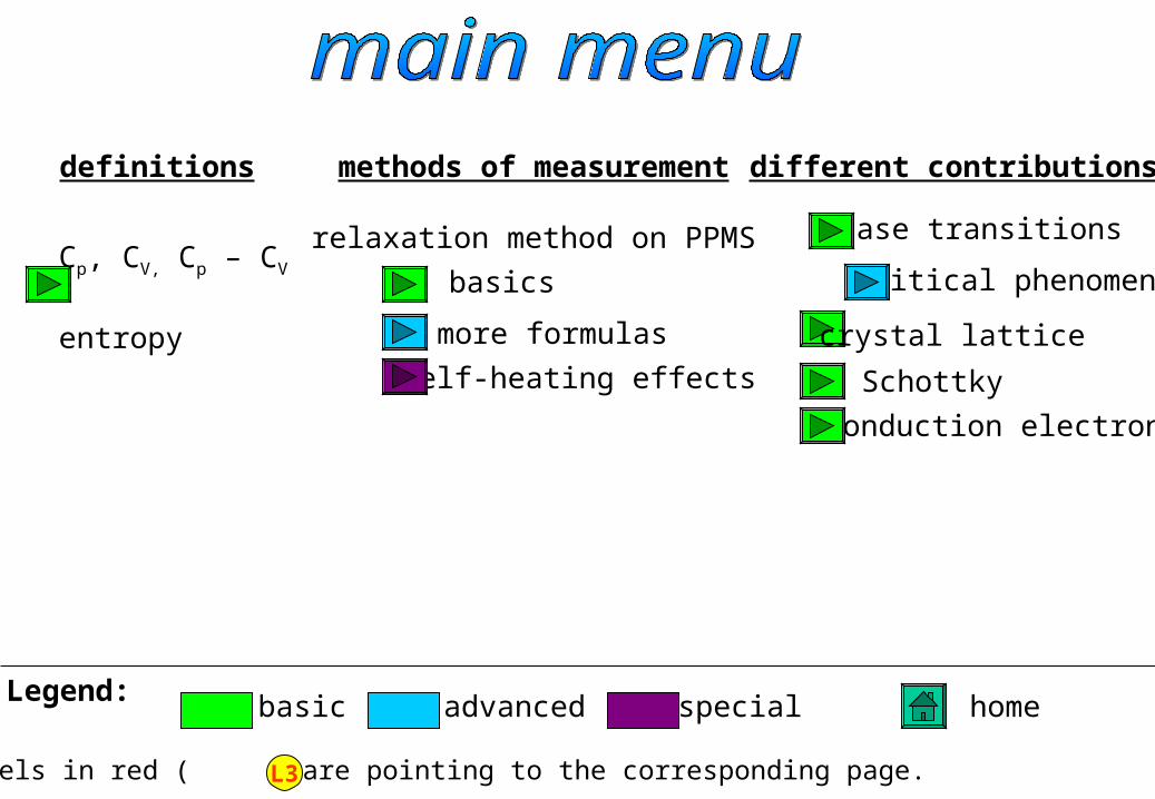
definitions methods of measurement different contributions

Cp, CV, Cp – CV

entropy

Legend: basic advanced special

relaxation method on PPMS

basics

more formulas

self-heating effects

home

phase transitions

critical phenomena

crystal lattice

Schottky

conduction electrons

Formula labels in red ( )are pointing to the corresponding page.L3

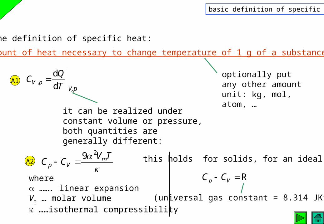
Here is the definition of specific heat:

the amount of heat necessary to change temperature of 1 g of a substance by 1 K

T

QC pV d

d,

V,p

TV

CC mVp

29

where ……. linear expansionVm … molar volume ……isothermal compressibility

optionally put any other amount unit: kg, mol, atom, …

it can be realized under constant volume or pressure, both quantities are generally different:

A1

A2

basic definition of specific heat

this holds for solids, for an ideal gas

R Vp CC

(universal gas constant = 8.314 JK-1mol-1)

1

01 d)(

T

TC TTS

If we know the specific heat in the whole temperature range from zero up to certain temperature T1, the total entropy can be easily calculated by integration:

A3

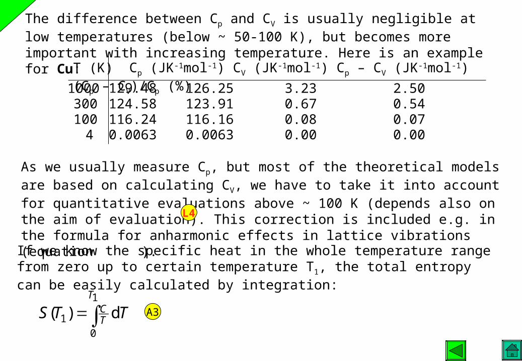
The difference between Cp and CV is usually negligible at low temperatures (below ~ 50-100 K), but becomes more important with increasing temperature. Here is an example for Cu:

T (K) Cp (JK-1mol-1) CV (JK-1mol-1) Cp – CV (JK-1mol-1) (Cp – CV)/Cp (%)

300100

1000

4

129.48 126.25 3.230.67123.91124.58

116.24 116.16 0.080.000.00630.0063

2.500.540.070.00

As we usually measure Cp, but most of the theoretical models are based on calculating CV, we have to take it into account for quantitative evaluations above ~ 100 K (depends also on the aim of evaluation). This correction is included e.g. in the formula for anharmonic effects in lattice vibrations (equation ).L4

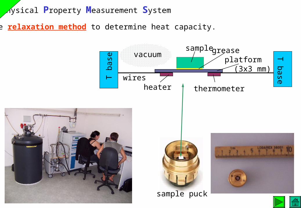
Physical Property Measurement System

uses the relaxation method to determine heat capacity.

sample greaseplatform (3x3 mm)

heater thermometer

wires

vacuum T baseT

bas

e

sample puck

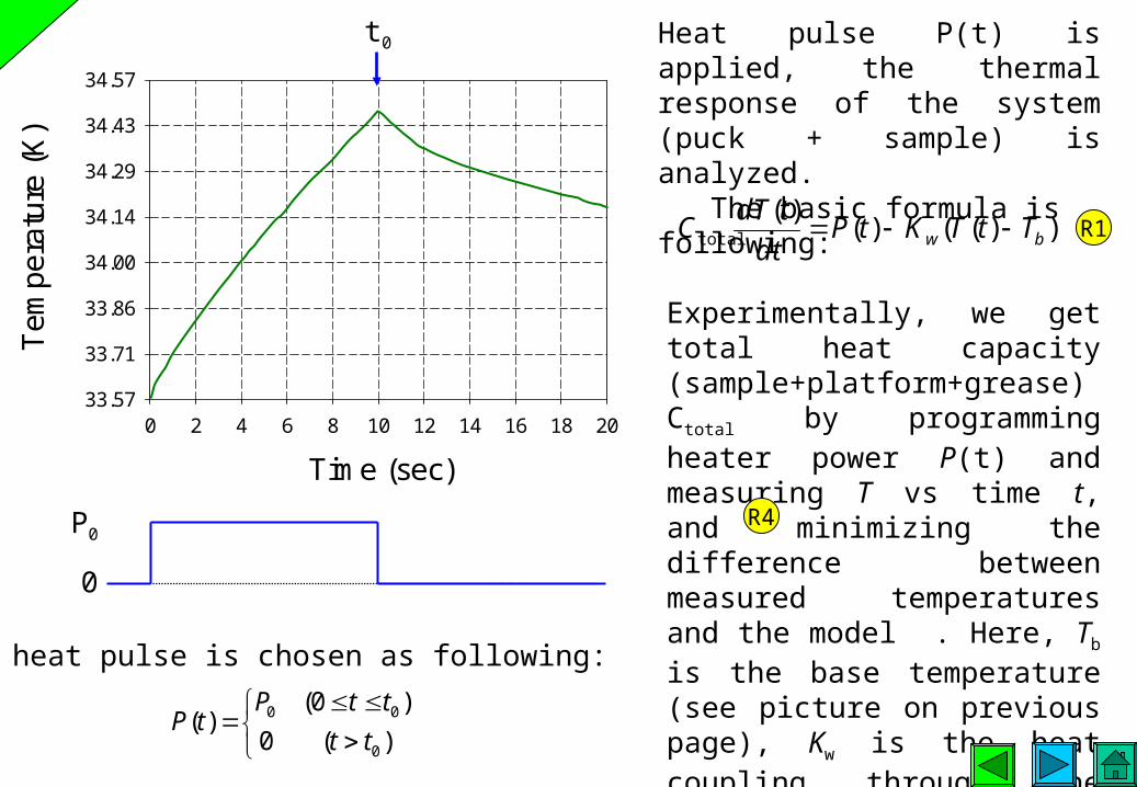
Time (sec)

0 2 4 6 8 10 12 14 16 18 20

Te

mp

era

ture

(K

)

33.57

33.71

33.86

34.00

34.14

34.29

34.43

34.57

))(()()(

total bw TtTKtPdt

tdTC

)(0

)0()(

0

00

tt

ttPtP

t0 Heat pulse P(t) is applied, the thermal response of the system (puck + sample) is analyzed. The basic formula is following:

R1

Experimentally, we get total heat capacity (sample+platform+grease) Ctotal by programming heater power P(t) and measuring T vs time t, and minimizing the difference between measured temperatures and the model . Here, Tb is the base temperature (see picture on previous page), Kw is the heat coupling through the wires.The heat pulse is chosen as following:

P0

0

R4

)()()(

)()()()()(

sample

platform

tTtTKdt

tdTC

tTtTKTtTKtPdt

tdTC

psgs

psgbpwp

Time (sec)

0 2 4 6 8 10 12 14 16 18 20

Te

mp

era

ture

(K

)

33.57

33.71

33.86

34.00

34.14

34.29

34.43

34.57

t0

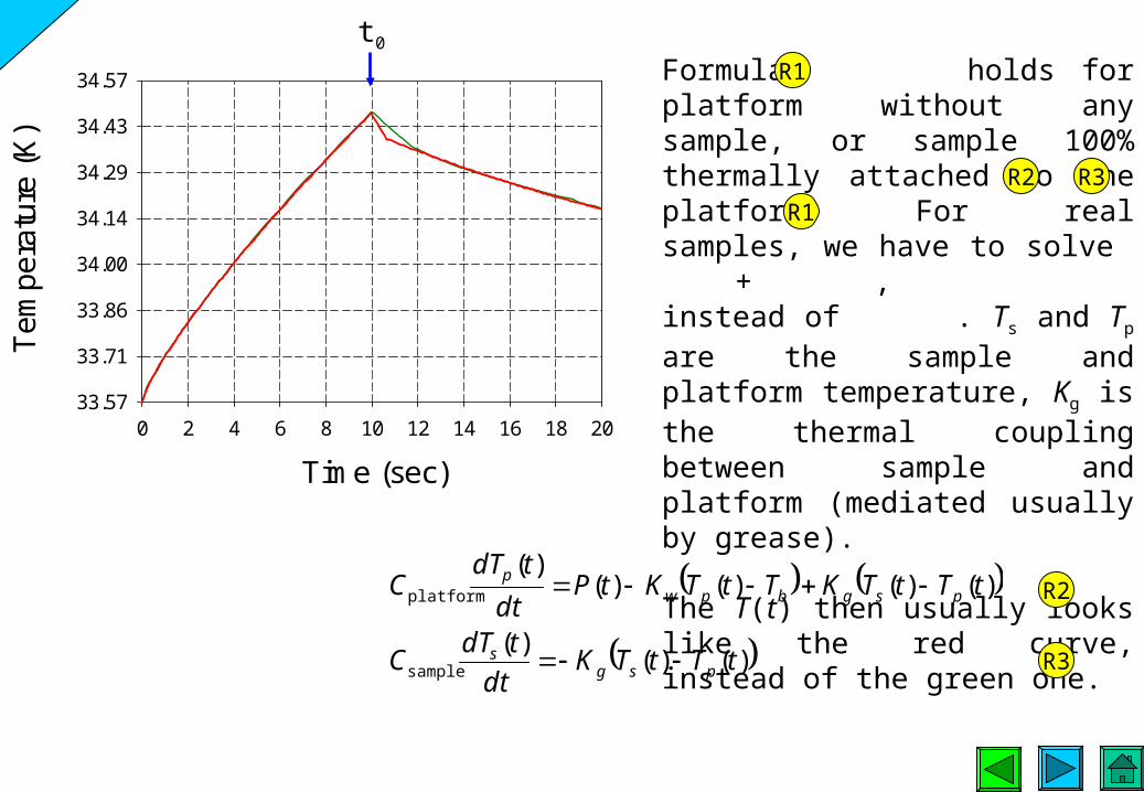
Formula holds for platform without any sample, or sample 100% thermally attached to the platform. For real samples, we have to solve + , instead of . Ts and Tp are the sample and platform temperature, Kg is the thermal coupling between sample and platform (mediated usually by grease).

The T(t) then usually looks like the red curve, instead of the green one.

R1

R2

R1

R3

R2

R3

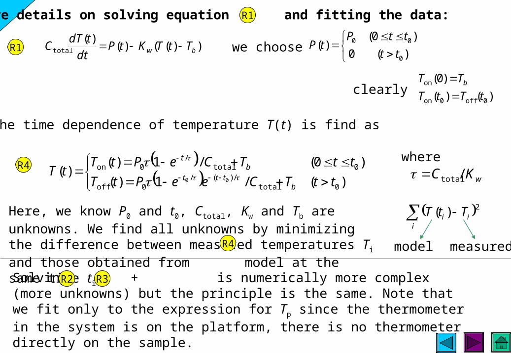
More details on solving equation and fitting the data:R1

))(()()(

total bw TtTKtPdt

tdTC

)(/1)(

)0(/1)()(

0total/)(/

0off

0total/

0on

00 ttTCeePtT

ttTCePtTtT

bttt

bt

)(0

)0()(

0

00

tt

ttPtP

),()(

)0(

0off0on

on

tTtT

TT b

R1 we choose

clearly

Then the time dependence of temperature T(t) is find as

wKC /totalwhere

R4

Here, we know P0 and t0, Ctotal, Kw and Tb are unknowns. We find all unknowns by minimizing the difference between measured temperatures Ti and those obtained from model at the same time ti.

R4

i

ii TtT 2)(

measuredmodel

Solving + is numerically more complex (more unknowns) but the principle is the same. Note that we fit only to the expression for Tp since the thermometer in the system is on the platform, there is no thermometer directly on the sample.

R2 R3

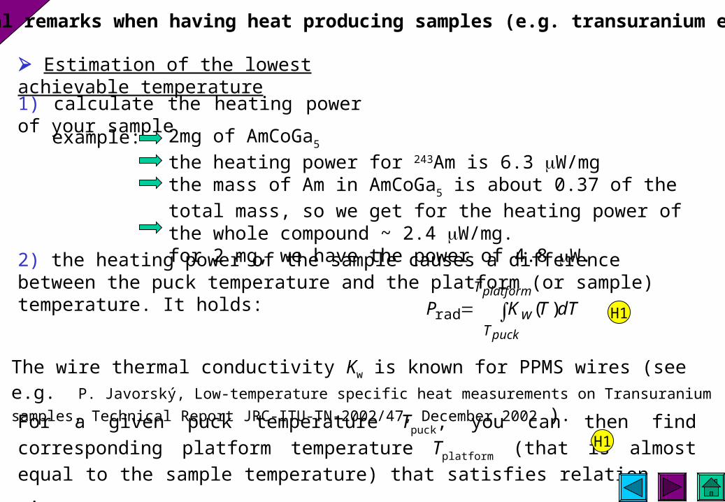
Special remarks when having heat producing samples (e.g. transuranium elements).

Estimation of the lowest achievable temperature

1) calculate the heating power of your sample

2) the heating power of the sample causes a difference between the puck temperature and the platform (or sample) temperature. It holds:

2mg of AmCoGa5

the heating power for 243Am is 6.3 W/mg the mass of Am in AmCoGa5 is about 0.37 of the total mass, so we

get for the heating power of the whole compound ~ 2.4 W/mg.for 2 mg, we have the power of 4.8 W.

example:

platform

puck

T

Tw dTTKP )(rad H1

The wire thermal conductivity Kw is known for PPMS wires (see e.g. P. Javorský, Low-temperature

specific heat measurements on Transuranium samples, Technical Report JRC-ITU-TN-2002/47, December 2002 ).

For a given puck temperature Tpuck, you can then find corresponding platform temperature

Tplatform (that is almost equal to the sample temperature) that satisfies relation .H1

Corrections for the temperature gradients

During the measurement, the temperature is measured on the puck and on the platform, the latter one is assumed to be the sample temperature as well as the temperature of all the wires. In reality, if your sample produces a heat, the sample is at higher temperature, and the wires at lower temperature. To correct for this, we can apply following procedure:

1) From the data file calculate the sample heat capacity as usual (i.e. subtract addenda), Csample(Tplatform) in J/K take the Tplatform (shown as sample temperature), Tpuck

and sample coupling .

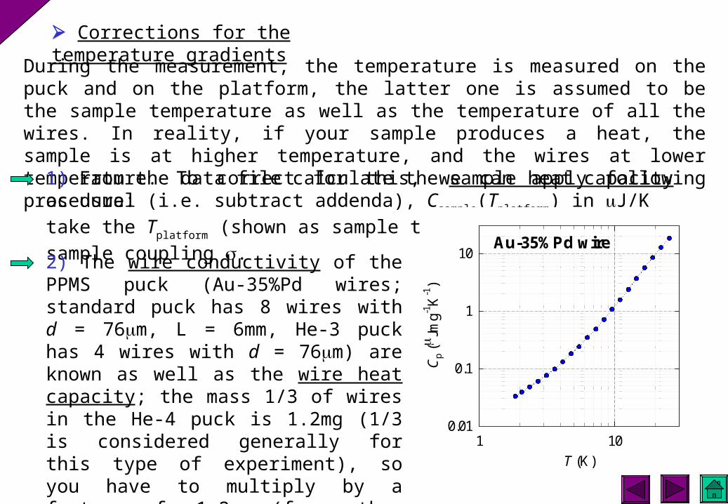
2) The wire conductivity of the PPMS puck (Au-35%Pd wires; standard puck has 8 wires with d = 76m, L = 6mm, He-3 puck has 4 wires with d = 76m) are known as well as the wire heat capacity; the mass 1/3 of wires in the He-4 puck is 1.2mg (1/3 is considered generally for this type of experiment), so you have to multiply by a factor of 1.2. (for other pucks, e.g. He-3, recalculate Cp according to number, material and diameter of the wires). T (K)

1 10C

p (

Jmg-1

K-1

)0.01

0.1

1

10Au-35%Pd wire

3) Calculate for all temperatures.wg KK

100

4) Calculate the radiation power using for all Tplatform.H1

5) Calculate the corrected sample and wire temperatures:

g

radKP

platformsample TT w

radK

Pplatformwire TT

4 H2

6) The error due to the fact that sample is more hot:

)()(1 platformsamplesamplesample TCTCC

If the Cp(T) increases with increasing temperature (usual case), then this correction means

that the heat capacity Csample at Tplatform (that one you get in your data file) is higher than it

should be. Applying this correction you diminish it.

)()(2 platformwirewirewire TCTCC 7) The error due to the fact that the wires are at lower temperature

As the Cwire decreases with T, this correction makes your Csample data larger because

originally the PPMS subtracted too high contribution for the wires than it really was.

8) Add both corrections, get corrected Csample(Tplatform) or Csample(Tsample) in J/K and

recalculate to J/mol.K or other units.

H3

H4

Generally, one can observe phase transitions of

first-order type; in an ideal case we observe here a discontinuity in entropy.

second-order type; in an ideal case we observe here a discontinuity in heat capacity.

These phase transitions can be of different origin, e.g.

the critical point of a substance (such as water) the transition between crystal structures the magnetic phase transition the trasition from ordered to disordered in liquid crystals the transition from superconducting to normal the transition from superfluid to normal fluid ….

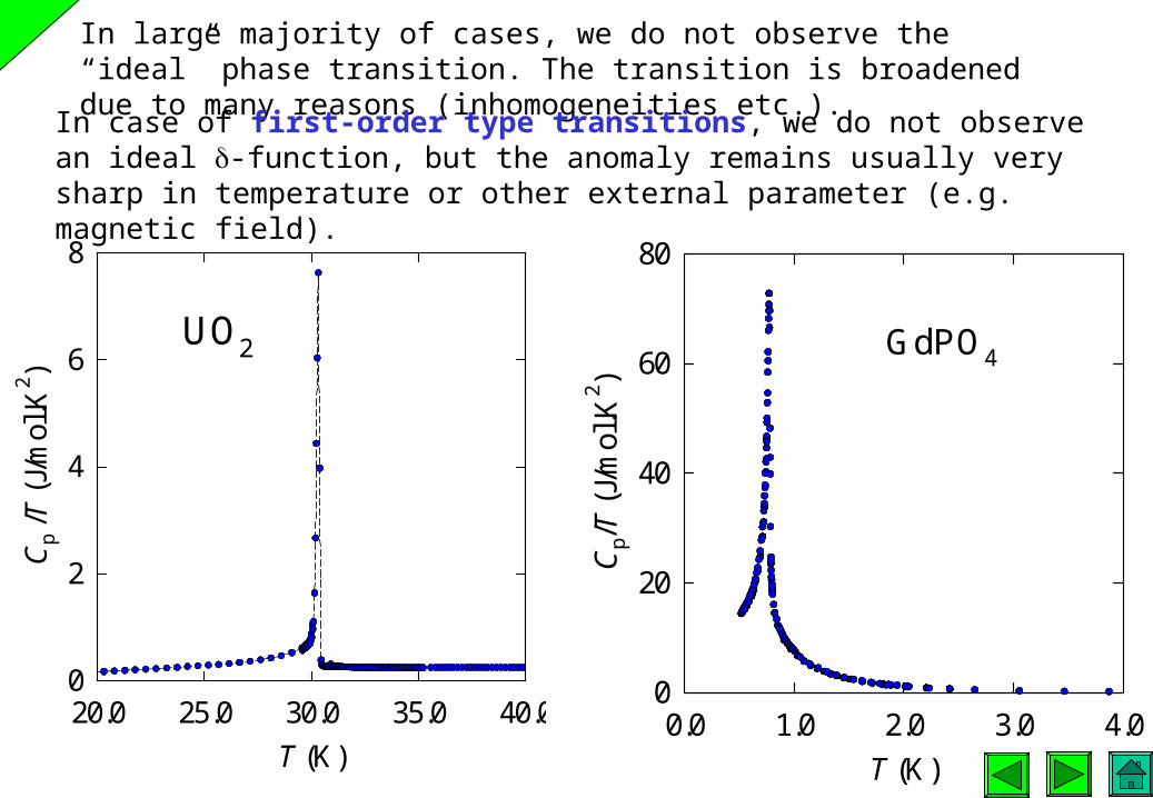
In large majority of cases, we do not observe the “ideal” phase transition. The transition is broadened due to many reasons (inhomogeneities etc.).

T (K)

20.0 25.0 30.0 35.0 40.0

Cp

/ T (

J/m

ol.K

2 )

0

2

4

6

8

UO2

T (K)

0.0 1.0 2.0 3.0 4.0

Cp/

T (

J/m

ol.K

2 )

0

20

40

60

80

GdPO4

In case of first-order type transitions, we do not observe an ideal -function, but the anomaly remains usually very sharp in temperature or other external parameter (e.g. magnetic field).

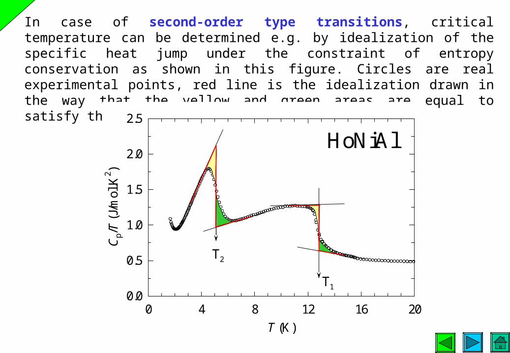
In case of second-order type transitions, critical temperature can be determined e.g. by idealization of the specific heat jump under the constraint of entropy conservation as shown in this figure. Circles are real experimental points, red line is the idealization drawn in the way that the yellow and green areas are equal to satisfy the entropy conservation.

T (K)

0 4 8 12 16 20

Cp/

T (

J/m

ol.K

2 )

0.0

0.5

1.0

1.5

2.0

2.5

HoNiAl

T2

T1

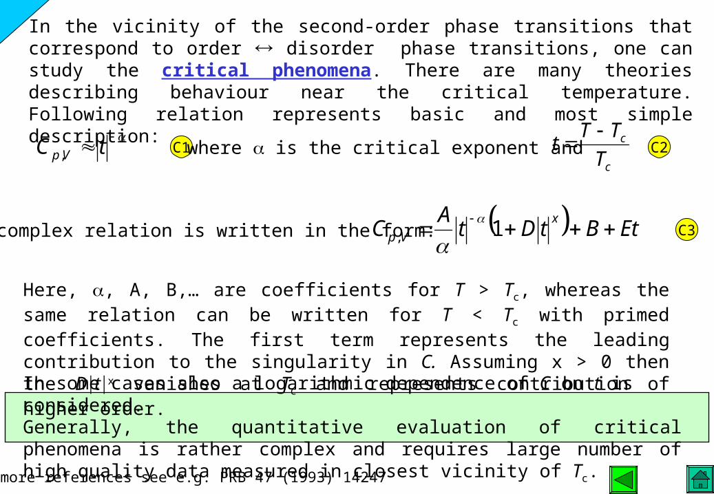
In the vicinity of the second-order phase transitions that correspond to order disorder phase transitions, one can study the critical phenomena. There are many theories describing behaviour near the critical temperature. Following relation represents basic and most simple description:

tC Vp, C1 where is the critical exponent andc

c

T

TTt

C2

C3More complex relation is written in the form: EtBtDtA

Cx

Vp 1,

Here, , A, B,… are coefficients for T > Tc, whereas the same relation can be written for T < Tc with primed coefficients. The first term represents the leading contribution to the singularity in C. Assuming x > 0 then the Dtx vanishes at Tc and represents contribution of higher order.In some cases also a logarithmic dependence of C on t is considered.Generally, the quantitative evaluation of critical phenomena is rather complex and requires large number of high quality data measured in closest vicinity of Tc.

for more references see e.g. PRB 47 (1993) 14247

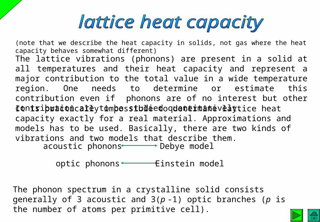
The lattice vibrations (phonons) are present in a solid at all temperatures and their heat capacity and represent a major contribution to the total value in a wide temperature region. One needs to determine or estimate this contribution even if phonons are of no interest but other contribution are to be studied quantitatively.

(note that we describe the heat capacity in solids, not gas where the heat capacity behaves somewhat different)

The phonon spectrum in a crystalline solid consists generally of 3 acoustic and 3(p -1) optic branches (p is the number of atoms per primitive cell).

It is practically impossible to determine lattice heat capacity exactly for a real material. Approximations and models has to be used. Basically, there are two kinds of vibrations and two models that describe them.

acoustic phonons

optic phonons

Debye model

Einstein model

Einstein model

N

iT

T

Ve

e

TC

12/iE

/iE2

iEAB

)( 1Nk

dxe

exTC

T

x

x

V )1(

N3k /

02

43

DAB

D

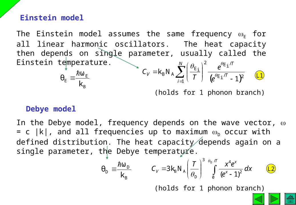
The Einstein model assumes the same frequency E for all linear harmonic oscillators. The heat capacity then depends on single parameter, usually called the Einstein temperature.

B

EE k

ωθ

L1

Debye model

In the Debye model, frequency depends on the wave vector, = c |k|, and all frequencies up to maximum D occur with defined distribution. The heat capacity depends again on a single parameter, the Debye temperature.

(holds for 1 phonon branch)

L2B

DD k

ωθ

(holds for 1 phonon branch)

at T << D, simplifies to 33D

3 θ R234 TTCV

3D β

R234)atoms (θ

NN

In principle, one can take different characteristic parameter (E or D) for every phonon branch. Nevertheless, one can assume more simplifications in most cases. For example, the heat capacity of acoustic phonons is usually well described by a single D and the optic phonons can be also usually well grouped.For lattice with single atom in the unit cell, there are only 3 acoustic branches and the lattice heat capacity is well described by (with the numerical pre-factor 9 instead of 3).

L2

L3

(holds for 1 atom in unit cell = 3 phonon branches)

As the contribution of optic vibrations to the heat capacity at these low temperatures is much smaller than that of acoustic ones, can be used for majority of materials at low T.

(usually below 10K as D ~ 100K)

L3

useful formula when relating to D:

Low temperatures

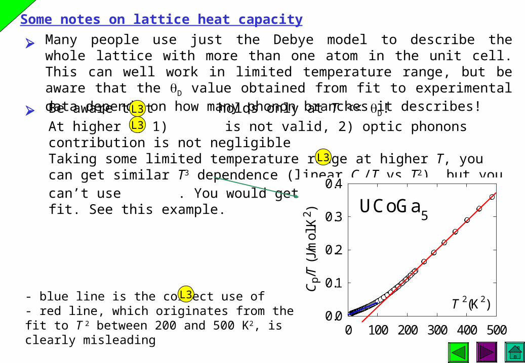
Many people use just the Debye model to describe the whole lattice with more than one atom in the unit cell. This can well work in limited temperature range, but be aware that the D value obtained from fit to experimental data depends on how many phonon branches it describes!

Some notes on lattice heat capacity

Be aware that holds only at T << D!At higher T, 1) is not valid, 2) optic phonons contribution is not negligible Taking some limited temperature range at higher T, you can get similar T3 dependence (linear Cp/T vs T2), but you can’t use . You would get wrong values from the fit. See this example.

L3

L3

L3

T 2(K2)

0 100 200 300 400 500

Cp/

T (

J/m

ol.K

2 )0.0

0.1

0.2

0.3

0.4

UCoGa5

- blue line is the correct use of - red line, which originates from the fit to T 2 between 200 and 500 K2, is clearly misleading

L3

Ti1

1

Anharmonicity effects

Equations to are valid in the harmonic approximation only.

C.A. Martin, J.Phys.: Condens. Matter 3 5967 (1991)

L1 L3

The anharmonicity becomes more important at higher temperatures (~ 200 K and above), depending strongly also on the given lattice properties. To calculate the heat capacity in such a case is rather complex, so one tries to use simple approximations. Such simplification is given by term

that should multiply lattice CV for every branch. This correction involves also the Cp-CV difference that also becomes important at higher T. The parameters i can be generally different for different branches, but are often fixed to one common value for simplicity.

For theoretical background see e.g.:

L4

2k/

2k/B

k/

k/2B

ABB

B

B

B )k/()k/(Nk

TEi

TEii

TEi

TEii

Schottkyi

i

i

i

en

eTEn

en

eTEnC

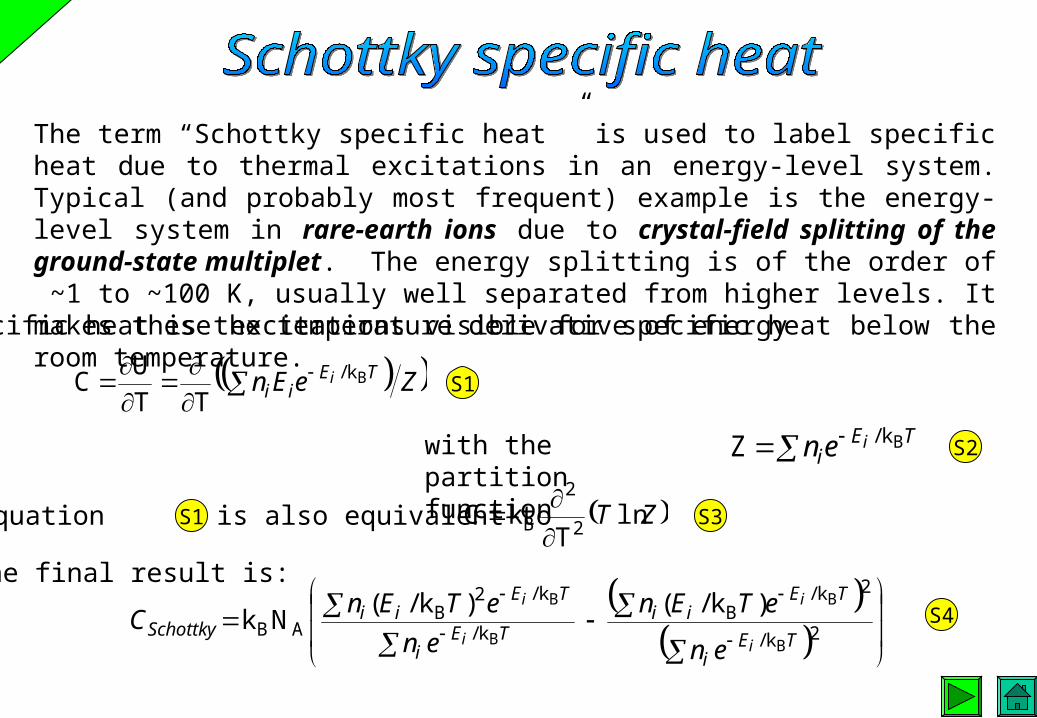
The term “Schottky specific heat ” is used to label specific heat due to thermal excitations in an energy-level system. Typical (and probably most frequent) example is the energy-level system in rare-earth ions due to crystal-field splitting of the ground-state multiplet. The energy splitting is of the order of ~1 to ~100 K, usually well separated from higher levels. It makes these excitations visible for specific heat below the room temperature.The specific heat is the temperature derivative of energy

ZeEn TEii

i

Bk/

TT

UC S1

with the partition function

TEi

ien Bk/Z S2

S1The equation is also equivalent to ZT lnT

kC2

2

B S3

The final result is:

S4

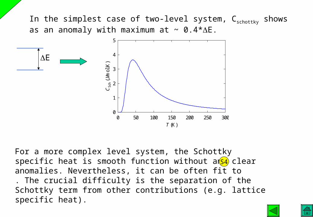
In the simplest case of two-level system, Cschottky shows as an anomaly with maximum at ~ 0.4*E.

E

T (K)

0 50 100 150 200 250 300

CS

ch (

J/m

ol.K

)0

1

2

3

4

5

For a more complex level system, the Schottky specific heat is smooth function without any clear anomalies. Nevertheless, it can be often fit to . The crucial difficulty is the separation of the Schottky term from other contributions (e.g. lattice specific heat).

S4

TkT

TNU B

F T)kg(E

E

TNk

T

TNk

T

UC 2

BFF

2B

FBel

T)kg(EπC 2BF

231

el

F

BB

221

el ETk

NkπC F

F 2E

3N)g(E

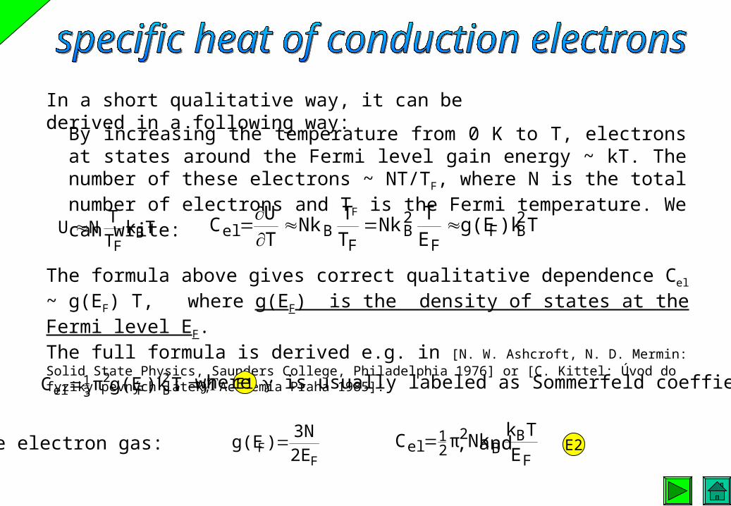
In a short qualitative way, it can be derived in a following way:

By increasing the temperature from 0 K to T, electrons at states around the Fermi level gain energy ~ kT. The number of these electrons ~ NT/TF, where N is the total number of electrons and TF is the Fermi temperature. We can write:

The formula above gives correct qualitative dependence Cel ~ g(EF) T, where g(EF) is the density of states at the Fermi level EF.The full formula is derived e.g. in [N. W. Ashcroft, N. D. Mermin: Solid State Physics, Saunders College, Philadelphia 1976] or [C. Kittel: Úvod do fyziky pevných látek, Academia Praha 1985]:

E1

For a free electron gas: , and E2

, where is usually labeled as Sommerfeld coeffiecient.

T2 (K2)

0 20 40 60 80 100

Cp/

T (

mJ/

mol

.K2 )

0

10

20

30

40

50

60

LuNiAl

Au

Cu

f.e.

exp

e γ

γ

m

*m

β

γ

2p βTγT/C

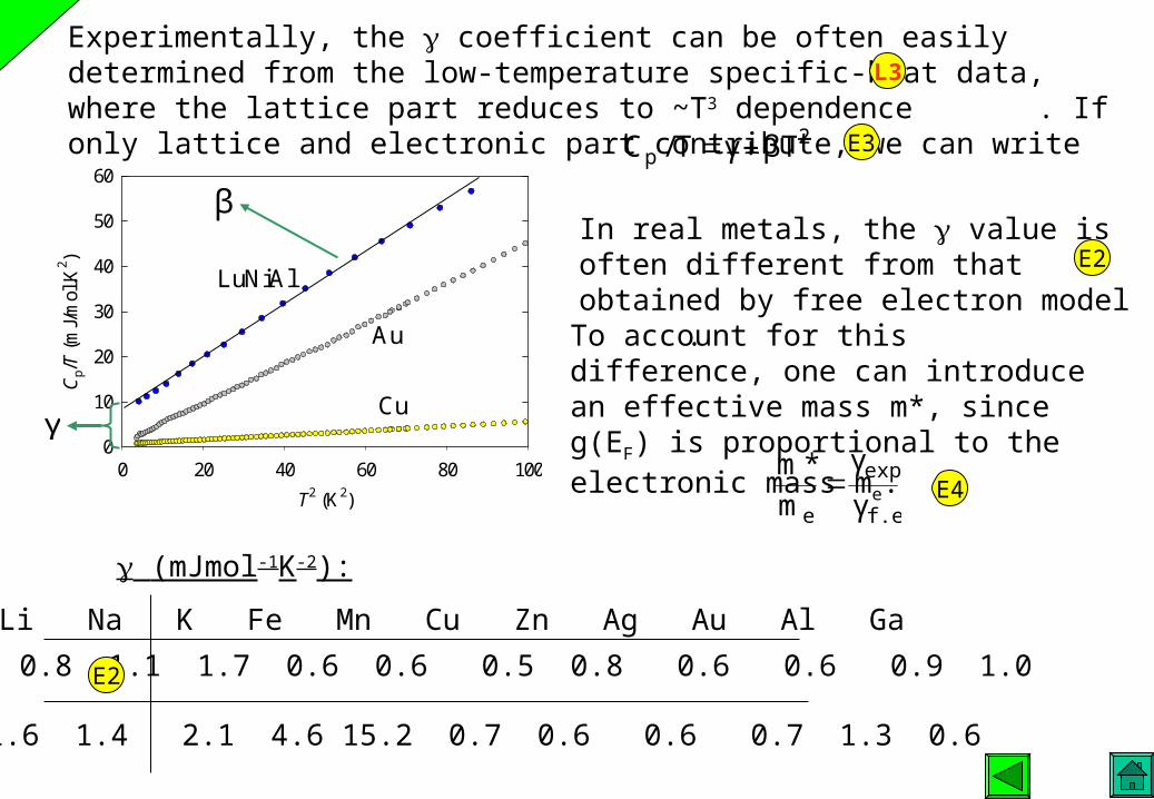
(mJmol-1K-2):

experiment 1.6 1.4 2.1 4.6 15.2 0.7 0.6 0.6 0.7 1.3 0.6

0.8 1.1 1.7 0.6 0.6 0.5 0.8 0.6 0.6 0.9 1.0

Li Na K Fe Mn Cu Zn Ag Au Al Ga

Experimentally, the coefficient can be often easily determined from the low-temperature specific-heat data, where the lattice part reduces to ~T3 dependence . If only lattice and electronic part contribute, we can write

L3

E3

In real metals, the value is often different from that obtained by free electron model .E2

E2

To account for this difference, one can introduce an effective mass m*, since g(EF) is proportional to the electronic mass me.

E4