Embed Size (px)
Citation preview

HAL Id: hal-00454445https://hal.archives-ouvertes.fr/hal-00454445v2
Submitted on 16 Feb 2011
HAL is a multi-disciplinary open accessarchive for the deposit and dissemination of sci-entific research documents, whether they are pub-lished or not. The documents may come fromteaching and research institutions in France orabroad, or from public or private research centers.
L’archive ouverte pluridisciplinaire HAL, estdestinée au dépôt et à la diffusion de documentsscientifiques de niveau recherche, publiés ou non,émanant des établissements d’enseignement et derecherche français ou étrangers, des laboratoirespublics ou privés.
Definition of spacing constraints for the car sequencingproblem
Aymeric Lesert, Gülgün Alpan, Yannick Frein, Stephane Noire
To cite this version:Aymeric Lesert, Gülgün Alpan, Yannick Frein, Stephane Noire. Definition of spacing constraints forthe car sequencing problem. International Journal of Production Research, Taylor & Francis, 2010,pp.1. �10.1080/00207540903469043�. �hal-00454445v2�
For Peer Review O
nly
Definition of spacing constraints for the car sequencing
problem
Journal: International Journal of Production Research
Manuscript ID: TPRS-2008-IJPR-0730.R2
Manuscript Type: Original Manuscript
Date Submitted by the Author:
15-Jul-2009
Complete List of Authors: Lesert, Aymeric; Laboratoire G-SCOP Alpan, Gulgun; Laboratoire G-SCOP, Grenoble Institute of Technology Frein, Yannick; Laboratoire G-SCOP, Grenoble Institute of Technology Noire, Stephane; PSA Peugeot Citroën
Keywords: ASSEMBLY LINE BALANCING, MIXED MODEL SEQUENCING
Keywords (user): SPACING CONSTRAINTS
http://mc.manuscriptcentral.com/tprs Email: [email protected]
International Journal of Production Research

For Peer Review O
nly
- 1 -
Definition of spacing constraints for the
car sequencing problem
Aymeric Lesert
2, Gülgün Alpan
2, Yannick Frein
2, Stéphane Noiré
1
1 PSA Peugeot Citroën, 45, rue Jean-Pierre Timbaud, 78307 Poissy Cedex,
2 G-SCOP, ENSGI-INPG,46 Avenue Félix Viallet, 38031 Grenoble Cedex,
[email protected], [email protected] , [email protected]
ABSTRACT: Car sequencing problem deals with the ordering of a list of vehicles to be produced on an
assembly line so that the overall capacity of each workstation is not exceeded. Some types of vehicles require
several time consuming operations to be done on a workstation and will naturally overload that workstation.
Such vehicles are spaced out in the sequence, by means of a set of spacing constraints, in order to cope with the
momentary increase of workload that they create. Two questions arise: which type of vehicles should be subject
to the spacing constraints and by which distance should they be spaced out in the sequence. In practice as well
as in the car sequencing literature, there does not exist a methodical way to answer the first question and the
existing methods for the second one is no longer adequate due to the increased diversity of cars produced in an
assembly line. In this paper, we propose two new methods to answer these questions with a special emphasis on
the first one. The performance of the proposed methods is illustrated using a real case study.
KEYWORDS: Spacing constraints, mixed model assembly lines, line balancing, car sequencing problem,
automotive industry
Page 1 of 60
http://mc.manuscriptcentral.com/tprs Email: [email protected]
International Journal of Production Research
123456789101112131415161718192021222324252627282930313233343536373839404142434445464748495051525354555657585960

For Peer Review O
nly
- 2 -
Introduction
A typical automotive assembly line is physically divided into more than a hundred
consecutive workstations. In each workstation, one or more operators perform a number of
tasks on each vehicle (see figure 1) using the parts and tools available. Every vehicle to be
produced goes through these serial workstations at the same speed and in the same order. Due
to this constant velocity, these assembly lines are also called the paced assembly lines. Time
spent by a vehicle in a workstation is called the cycle time. Physically this means that when
the thj vehicle in the sequence exits a given workstation the stj )1( + vehicle enters it and
spends a time equal to the cycle time in this station (see figure 1).
Assembly line balancing consists in assigning the operations to the workstations such
that the workload of each station is the most homogenous possible and the average time of the
tasks to be performed in every workstation does not exceed the cycle time (Scholl and Becker,
2006), (Becker and Scholl, 2006). In practice, for economical and technical reasons, duration
of some type of vehicles is allowed to exceed the cycle time at some. These vehicles overload
the related workstation since the operator needs more than the cycle time to complete the
tasks on the vehicle. The operator accumulates a delay since he now has less than the cycle
time to finish the next vehicle. If the following vehicles have high operation durations as well,
the operator cannot recover the delay. If the total delay becomes important and no recovery is
possible, either a utility worker is called up for help or the line is stopped.
[FIGURE 1 HERE]
These emergency solutions are costly and may also degrade the product quality. In
practice (Comby, 1996), (Baratou, 1998), (Joly, 2004), (Bernier and Frein, 2004), (Joly et. al.
2008) as well as in the car sequencing literature (for example, see (Burns and Daganzo, 1986),
(Tsai, 1992) and (Warwick and Tsang, 1995)) the vehicles which create overload are spaced
in the sequence. This is realized by spacing constraints.
A spacing constraint is defined by two data: a criterion and a ratio N/P. The criterion
represents an option or a combination of several options to be spaced. The ratio N/P
represents the maximum number (i.e. N) of vehicles with the criterion in a sliding window of
(P) vehicles in the sequence. If this ratio is well chosen and a sequence respecting the spacing
constraint is found, total utility work is minimized (Bolat and Yano, 1992a, 1992b). The
literature on the car sequencing problem is abundant. Here, we will not give a detailed
Page 2 of 60
http://mc.manuscriptcentral.com/tprs Email: [email protected]
International Journal of Production Research
123456789101112131415161718192021222324252627282930313233343536373839404142434445464748495051525354555657585960

For Peer Review O
nly
- 3 -
overview of this literature but we invite the interested readers to refer to the recent surveys by
(Solnon et. al., 2007) and (Boysen et. al. 2009) which give a complete review of the existing
work.
The existing literature which deals with the car sequencing problem assume that the
spacing constraints are given and correctly defined. However, the quality of the car sequence
is highly dependent on a correct definition of the spacing constraints (Bolat and Yano,
1992b). In practice, the criteria of the spacing constraints are defined based on experience and
the ratios, N/P, are often deduced by the number of vehicles to produce. In the current context
of the automobile industry, the diversity of vehicles which can be produced on a mixed model
assembly line is tremendous and the definition of spacing constraints is a very complicated
task (Lesert and al., 2007). To the best of our knowledge, no work exists in the literature on
the selection of the criteria of the spacing constraints and very few studies have been reported
on the calculation of N/P (Giard and Jeunet, 2006), (Yano and Rachamadugu, 1991), (Bolat
and Yano, 1992a), (Bolat and Yano, 1992b).
In this article, we will describe a model for the definition of spacing constraints to
answer the following questions: which options should be spaced (i.e. definition of the criteria)
and by which distance (i.e. calculation of kk PN ,where k is the index of the constraint) such
that the emergency situations which may occur on the assembly line are captured better by the
spacing constraints. To achieve these objectives we will first analyse, in section 2, the
movements of an operator in his workstation. This analysis gives us valuable information on
how an operator accumulates delay. Section 3 is dedicated to the definition of the criteria of
the spacing constraint while section 4 describes how to choose the values Nk and Pk, for all k.
In section 5, the proposed method is compared to the current methods and its performance is
illustrated via some numerical results based on generated data. Section 6 presents a real case
study. Finally, section 7 concludes the article.
Mathematical model of a delay
As mentioned before, if an operator accumulates an important delay, a utility worker is
called up for help. In order to model the accumulation of the delay we first observe the
movements of an operator.
Page 3 of 60
http://mc.manuscriptcentral.com/tprs Email: [email protected]
International Journal of Production Research
123456789101112131415161718192021222324252627282930313233343536373839404142434445464748495051525354555657585960

For Peer Review O
nly
- 4 -
Movement of an operator in his workstation
A typical automotive assembly line is a paced assembly line where the vehicles to
produce move from one workstation to the other on a constant speed conveyor belt ( x
meters/min). In the assembly line under study, the workstations are equally sized. The time
elapsed between the entry and exit of a vehicle in a workstation is hence constant and referred
to as the cycle time, cycleT . During cycleT , a vehicle travels a distance of cycleTx. meters. This is
the length of the workstation. Without loss of generality, we will use time metrics (e.g. cycleT )
to describe space limitations (e.g. cycleTx. ) as seen in figure 2. Space metrics can be found by a
simple conversion using the speed of the conveyor belt.
In practice, the operator may utilize a space greater than the length of his workstation.
The real boundaries of workstation i is hence delimited by a lower limit, iMin and an upper
limit, iMax as shown in figure 2. iMin and iMax are calculated based on the technical constraints
of tools used in the workstation and the specificities of the neighboring stations (i.e. the
operator should not bother the neighbor operators). iMin is always negative or null. And, iMax
is always greater than or equal to cycleT . Here on, the term workspace will be used to refer to
the practical boundaries of a workstation. In figure 2, the operator escorts each vehicle during
the assembly task (illustrated by horizontal bars) and then walks back upstream to treat the
next vehicle (illustrated by arrows). If the operator is ahead of his time, he may start working
on a vehicle before it actually enters the workstation (case of vehicle 2 in figure 2). Similarly,
if he has accumulated some delay, he may continue working on a vehicle beyond his own
workstation (case of vehicles 2 and 3 in figure 2).
[FIGURE 2 HERE]
When an operator can not complete all assembly tasks within the workspace (case of
vehicle 4 in figure 2), one of the following solutions can be used:
(i) The operator can stop the line to finish his job and restart the line afterwards (Toyota’s
ANDON1 method) (see Tsaï (1992) and Kim (2001)) (ii) A utility worker can be called up to
complete the unfinished work when the vehicle exits the workspace (Giard and Jeunet, 2006),
(Bolat and Yano, 1992a, 1992b). (iii) The utility worker treats a complete vehicle which
cannot be completed in the workspace (Giard and Jeunet, 2006).
1 ANDON : little lantern (In Japanese). A warning light is switched on above the operator who stops the line.
Page 4 of 60
http://mc.manuscriptcentral.com/tprs Email: [email protected]
International Journal of Production Research
123456789101112131415161718192021222324252627282930313233343536373839404142434445464748495051525354555657585960

For Peer Review O
nly
- 5 -
In this article, we will use the third approach since it satisfies the quality requirement
that an operator, who starts an assembly task on a vehicle, completes the task to avoid some
operations to be forgotten. Based on this hypothesis, the vehicle 4 in figure 2 will completely
be treated by a utility worker2 as soon as it enters the workspace. The operator can then
recover his delay by skipping the 4th
vehicle and handles the 5th
vehicle.
Mathematical model of the movements of an operator
An efficient spacing constraint is the one which is capable of smoothing the workload
of the operators such that the number of times the utility workers are summoned is minimal,
given that the constraint is respected in the car sequence. To model the movements of an
operator and hence the solicitation of a utility worker we will use the following notations:
jiT , : The duration of operations on vehicle j at workstation i
,i jD : The starting time of operations on vehicle j at workstation i
jiF , : The ending time of operations on vehicle j at workstation i.
jiS , : A flag which signals the presence of an important delay. , 1i jS = if the operator at
workstation i requires help for vehicle j and , 0i jS = otherwise.
We will also assume that: (i) Operators can treat all vehicles j in their workstation i,
i.e. ( ),i i i jj
Max Min Max T− ≥ , (ii) Operators do not face any technical (e.g. breakdown of a
screw driver) or logistic problems (e.g. missing parts), (iii) Utility workers are summoned
early enough to take in charge the vehicle requiring an intervention, (iv) The pool of utility
workers is sufficiently dimensioned to fulfil every alert, (v) The walk-back time of the
operator is not explicitly modelled: the return time being rather fast compared to the cycleT we
considered it as a fixed value and included it in the duration of operations jiT , . Such
simplifications are commonly used in the literature (see Bard et. al. (1992) for infinite return
velocities and Bolat et. al. (1994) for fixed durations added to station times). We note that in
the literature, there exist studies which explicitly model the finite return velocities. The
interested reader can refer to the work by Klampfl et. al. (2006) which addresses the
workstation layout optimization issues in order to minimize the walk-back and waiting time
of the operator in a mixed model assembly line context.
2 In certain assembly lines the alarm systems exist to warn the utility worker in time for an upcoming
Page 5 of 60
http://mc.manuscriptcentral.com/tprs Email: [email protected]
International Journal of Production Research
123456789101112131415161718192021222324252627282930313233343536373839404142434445464748495051525354555657585960

For Peer Review O
nly
- 6 -
Based on the above notations and assumptions, the solicitation of a utility worker for a
vehicle j at a workstation i, is expressed by equation (1).
iDi ∀= , 01,
, , ,i j i j i jF D T= +
iji
iji
ji MaxF
MaxF
if
ifS
>
≤
=,
,
,1
0
( )( )
>∀−
=−=
−
−−1, ,
else ,
0 if ,
1,
1,1,
, jiTDMinMax
STFMinMaxD
cyclejii
jicyclejii
ji
(1)
As noted in equation (1), ,i jD depends on the initial location of the operator: For the first
vehicle of the day, 1j = , the operator starts at the beginning of his work space : i.e. 01, =iD .
For the rest of the vehicles (i.e. j>1), the first line in the equation of ,i jD refers to the case
when the operator can treat the previous vehicle without help (i.e. 01, =−jiS ). In this case, the
reference for the ending time of operations on the (j-1)th
vehicle is the 1, −jiF . Since a new
vehicle arrives to the workstation every cycleT units of time, cycleji TF −−1, gives the point where
the operator can catch up the next vehicle in his work space. If icycleji MinTF ≤−−1, then the
operator has time to walk back up to the extreme boundaries of his workstation before the jth
vehicle arrives to his workstation (i.e. iji MinD =, ). If icycleji MinTF >−−1, the jth
vehicle has
already crossed the practical boundaries of the workstation and the operator can start treating
the jth
vehicle from cyclejiji TFD −= −1,, on. The second line of the equation for ,i jD expresses
the fact that the vehicle (j-1) is skipped (i.e. it is taken in charge by the utility worker). In this
case the ending time of the operations for (j-1)th
vehicle corresponds to 1, −jiD since the regular
operator does not treat this vehicle. He can walk upstream to take in charge the jth
vehicle.
The logic of calculations is the same as before with 1, −jiD taken as the ending time of
operations for the previous vehicle.
In this model, only a vehicle having ,i j cycleT T> (i.e. a work intensive vehicle) can induce
an emergency alarm. A vehicle having cycleji TT <, , on the other hand, may be scheduled after a
work intensive vehicle to help the operator to recover the accumulated delay. Hence the use of
problematic vehicle
Page 6 of 60
http://mc.manuscriptcentral.com/tprs Email: [email protected]
International Journal of Production Research
123456789101112131415161718192021222324252627282930313233343536373839404142434445464748495051525354555657585960

For Peer Review O
nly
- 7 -
a utility worker can be avoided. We note that, the above method can directly be used to find a
car sequence which minimizes the number of times the utility workers are called up. Such an
approach has been tested by (El Hadj-Khallaf , 2006) and proves to give promising results
compared to classical car sequencing methods (Thomopoulos, 1967), (Tsai, 1992), (Kim,
2001). However, there are some disadvantages of directly applying such approaches: First of
all, this approach requires a significant amount of data to be collected on operation times,
worker movements, the characteristics of workstations and the tasks (Boysen et. al., 2009).
This makes it inconvenient for industrial applications. Secondly, the car manufacturers such
as PSA Peugeot Citroën have already their car sequencing optimization tools which are based
on the use of the spacing constraints and the cost of modifications required on the information
system would be far beyond the potential profits. Therefore, in this paper, we propose to
improve the current methods to facilitate the definition of good quality spacing constraints.
A measure of the quality of a car sequence
We recall that the objective of constraining a car sequence using spacing constraints is
to have a smooth workload for the operators and hence to avoid the solicitation of utility
workers. When respected in the construction of the car sequence, a good spacing constraint
should attain this objective. In order to measure how well the spacing constraints are
respected, we use the indicator, kcI , given in equation (2) which counts the number of
vehicles which do not respect the spacing constraint k (denoted kc , here after), (Joly, 2005).
This function is very similar to the one proposed by (Fliedner and Boysen, 2008) and provides
the same evaluation for a given sequence.
∑ ∑= +−=
+−∗=
tot
k
k
Q
j
j
Pjlklkkjc xNxI
1 1,, 1,0,maxmin
(2)
totQ , the number of vehicles in the sequence,
kk PN , the ratio of kc ,
1, =kjx if the vehicle at position j in the car sequence has the criterion of kc , 0 otherwise.
Figure 3 illustrates the calculation of kcI for which the criterion is the “luxury
vehicles” and the ratio is 1/5. Given the sequence of vehicles, every sliding window of 5
Page 7 of 60
http://mc.manuscriptcentral.com/tprs Email: [email protected]
International Journal of Production Research
123456789101112131415161718192021222324252627282930313233343536373839404142434445464748495051525354555657585960

For Peer Review O
nly
- 8 -
vehicles is observed. Each violation of the constraint by a “luxury vehicle” will result in a 1
and no violation will result in 0. The vehicles which don’t respect the ratio are counted once
(circled in the figure). For this sequence, the number of violations is 2, and so 2=kcI .
[FIGURE 3 HERE]
The overall quality of a sequence is obtained by aggregating equation 2 for all spacing
constraints in a weighted sum as in equation 3. The weights, kω , are assigned to each
constraint according to its importance, by the line balancing staff and based on experience.
Some constraints are related to critical options and have to be met under all circumstances (a
high kω is assigned) while others can be violated if necessary (a low kω is assigned). Here,
we will assume that each constraint is equally important and 1=kω , k∀ . A good quality car
sequence is the one which has the minimal, scI .
∑=
=c
k
Nb
kckc II
1
*ω
Where cNb is the number of spacing constraints and kω is the weight of kc
(3)
In this article, we will use the indicator given in equation 3 to measure and to compare
the quality of car sequences.
Definition of the criteria of spacing constraints
One conclusion that we can draw from section 2 is that in order to minimize the
number of times a utility worker is called up, the work intensive vehicles are to be spaced out.
If we are able to characterize these vehicles, this will provide us with the criteria of a spacing
constraint. In this section, we will first explain how this characterization can be done. To this
end, we will first describe the relationship between a workstation and a spacing constraint.
In the classical car sequencing problem, (see for instance, (Parello et. al,1986), (Yano
et al. 1991), (Bolat and Yano, 1992a, 1992b) and (Kim, 2001)), a spacing constraint is defined
for a workstation with two kinds of vehicles: either the operator installs an option (e.g. CD
player, right hand side wheel, automatic gear, air bags, electrically powered windows, etc.) on
the vehicle and this creates a heavy workload, or the operator doesn’t install this option on the
vehicle and a low workload is observed. We will call this a “one option-two temporization”
problem.
Page 8 of 60
http://mc.manuscriptcentral.com/tprs Email: [email protected]
International Journal of Production Research
123456789101112131415161718192021222324252627282930313233343536373839404142434445464748495051525354555657585960

For Peer Review O
nly
- 9 -
This hypothesis might hold for the early periods of the automobile assembly lines.
However, in the current assembly lines, the diversity of vehicles is such that this point of view
is no longer valid: An operator may install several different options, variants of an option (e.g.
different engine specifications) or the same option with different quantities (eg. airbag only on
driver side or on both driver and passenger sides). This results in multiple temporizations in
the workstations.
Representation of the workload of an operator
The assembly tasks performed in a workstation are various and so are the duration of
the tasks. In figure 4, all vehicles j to be produced in workstation, i, are sorted in ascending
order of jiT , . The vehicles having the same jiT , are grouped together and represented
graphically. Throughout this article, this representation will be used to illustrate the workload
of an operator.
[FIGURE 4 HERE]
In the example workstation illustrated by figure 4, there are 5 different operation
times. There are 2 groups of vehicles with cycleji TT <, (in light grey) and 3 groups of vehicles
with ,i j cycleT T> (in dark grey). The workloads generated by the former groups of vehicles are
very low compared to the cycle time (leaving the operator idle) while the latter groups of
vehicles generate heavy workloads (and an inevitable delay for the operator).
The relationship between a workstation and the criterion of a spacing constraint
The challenge is to create a balanced car sequence such that the vehicles with
,i j cycleT T> are distanced from each other by inserting enough vehicles with cycleji TT <, in
between. As a consequence, we expect that a spacing constraint should be able to represent
the vehicles having ,i j cycleT T> . In order to quantify the capability of a criterion to represent the
work intensive vehicles of workstation i, we need to compare two subsets of vehicles
assembled in this workstation. Let, V be all the vehicles to be produced on the assembly line.
{ }k constraint spacing theof criterion thehas | vVvVkC ∈=
{ },|i i v cycleVp v V T T= ∈ >
Page 9 of 60
http://mc.manuscriptcentral.com/tprs Email: [email protected]
International Journal of Production Research
123456789101112131415161718192021222324252627282930313233343536373839404142434445464748495051525354555657585960

For Peer Review O
nly
- 10 -
where iVp ≠ ∅ and kVc ≠ ∅ . Indeed, a workstation with iVp = ∅ can accept any sequence of
vehicles without causing delays for the operator. Similarly, if kVc = ∅ , this means that there
are no vehicles to space.
Table 1 below summarizes 5 different relationships which exist between a workstation
i and a spacing constraint k . Depending on these relationships, a spacing constraint will be
more or less efficient to handle work overloads generated in a workstation. In the literature,
only the first type of relationship is considered (eg. Giard and Jeunet, 2006).
[Table 1. HERE ]
Each relationship of table 1 is illustrated via figures 5 to 9. In figures 5 to 9, the
diagram presented in section 3.1 is used to illustrate the workload of an operator in a
workstation. For illustration purposes, we present each workstation as a two-temporisation
station: vehicles creating no overloads (in light grey) and vehicles source of overloads (in
dark grey). Nevertheless, if a more detailed presentation is required, the diagram will look
like the one in figure 4. The cardinality of each set represents the quantity of each type of
vehicles. The slim bar under the diagram represents the vehicles characterized by the criterion
of a spacing constraint, i.e. ( )kcV . In figures 5 to 9, we consider the same spacing constraint
and 5 different workstations. We assume 1000=V and 500=kcV .
• In figure 5, k iVc Vp= meaning that all vehicles which overload workstation i are
exactly those who has the criterion of kc . Hence for this workstation, there is a perfect match
between the criterion of kc and the vehicles which should be spaced. In this case, we say that
« the workstation i is constrained by the spacing constraint k ».
[FIGURE 5 HERE]
• If k i iVc Vp Vp=I and k iVc Vp− ≠ ∅ as in figure 6, kc not only covers all vehicles which
overload workstation i but even more. The 400 vehicles out of 900 which do not overload the
workstation are also characterized by the same constraint. The constraint suggests that these
400 vehicles should be spaced in the sequence as well. In other words, kc over-estimates the
representation of troublesome vehicles. In this case, we say that « the workstation i is over-
constrained by the spacing constraint k ».
Page 10 of 60
http://mc.manuscriptcentral.com/tprs Email: [email protected]
International Journal of Production Research
123456789101112131415161718192021222324252627282930313233343536373839404142434445464748495051525354555657585960

For Peer Review O
nly
- 11 -
[FIGURE 6 HERE]
• Assume that i k kVp Vc Vc=I and i kVp Vc− ≠ ∅ as in figure 7. In the figure, only 500 out
of 700 work intensive vehicles are covered by kc in the workstation i and the remaining 200
is considered as vehicles which do not need to be spaced. In other words, kc under-estimates
the vehicles which overload workstation i. In this case, we say that « the workstation i is
under-constrained by the spacing constraint k ».
[FIGURE 7 HERE]
• If k iVc Vp ≠ ∅I , i k kVp Vc Vc≠I and k i iVc Vp Vp≠I , as in figure 8, then kc fails to cover
a part of the vehicles which overload workstation i. Indeed 50 vehicles among 520 with
,i j cycleT T> do not have the criterion of kc . Furthermore, it estimates that 30 vehicles which
create no peaks in the workstation should be distanced from each other in the car sequence. In
other words, kc can handle only a part of the potential problems. In this case, we say that
« the workstation i is impacted by the spacing constraint k ».
[FIGURE 8 HERE]
• And finally, if k iVc Vp = ∅I as in figure 9, then kc fails completely to identify the
target vehicles for this workstation. In this case, we say that « the workstation i is not
impacted by the spacing constraint k ».
[FIGURE 9 HERE]
One important conclusion that we draw from the above discussion is that the criterion
selected for a spacing constraint will have a different effect on each workstation: for some
workstations the criterion selected is a perfect match while for others it has no impact at all.
Unfortunately, the solution cannot be defining a criterion for every workstation. In an
automotive assembly line, there are several hundreds of workstations. Defining a spacing
constraint for each and every workstation is not reasonable since finding a car sequence which
satisfies each and every constraint will not be possible. In practice, the number of spacing
constraints (hence the number of criteria to define) is much less than the number of
workstations. For instance, in the case of the French car manufacturer PSA Peugeot Citroën
Page 11 of 60
http://mc.manuscriptcentral.com/tprs Email: [email protected]
International Journal of Production Research
123456789101112131415161718192021222324252627282930313233343536373839404142434445464748495051525354555657585960

For Peer Review O
nly
- 12 -
the number of spacing constraints is in the order of 10. In the rest of the section we propose a
method to evaluate the effects of different criteria on different workstations.
Hierarchy of relationships
The first question is how to rank the relationships among each other. Naturally, a good
criterion is the one which characterizes all vehicles with ,i j cycleT T> in workstation i . Then,
for the extreme cases (i.e. the first and the last relationship) the answer is straightforward.
The first relationship (figure 5) is perfect and will be ranked first while the fifth relationship
(figure 9) is without interest and hence will be ranked last. The difficulty is with the ranking
of the intermediary relationships (figure 10).
[FIGURE 10 HERE]
In figure 10, for a given workstation, we illustrate 3 different criteria to represent a
spacing constraint. If we have to select one of them, which one shall we take?
Three levels of impact factors
To answer the above question we propose 3 levels of impact factors. The first one
estimates the pertinence of the criterion of a spacing constraint with respect to a workstation
(in section 3.4.1). This value will then be aggregated over all criteria in order to obtain the
impact factor of the set of all spacing constraints on a workstation (see, section 3.4.2) and re-
aggregated once more with respect to all workstations in order to obtain a measure for the
whole assembly line (in section 3.4.3).
The impact factor of a criterion on a workstation
To evaluate the level of pertinence of the criterion of kc with respect to a workstation
i, we propose the impact factor, ,i kpI (equation 4).
( )( )
( )( ),
*i k
k ik ip
i i
Card Vc VpCard Vc VpI
Card Vp Card Vp=
II
Where k kVc V Vc= − , i iVp V Vp= − and )(YCard is the cardinality of the set Y
(4)
,i kpI varies between 0 and 1. « 0 » corresponds to a station not impacted by the spacing
constraint and « 1 » corresponds to a station constrained by the spacing constraint. In fact,
,i kpI is the product of two covering rates:
Page 12 of 60
http://mc.manuscriptcentral.com/tprs Email: [email protected]
International Journal of Production Research
123456789101112131415161718192021222324252627282930313233343536373839404142434445464748495051525354555657585960

For Peer Review O
nly
- 13 -
(i) ( )
( )k i
i
Card Vc Vp
Card Vp
I gives the percentage of vehicles with ,i j cycle
T T> that are covered
by the criterion of kc .
(ii) ( )
( )k i
i
Card Vc Vp
Card Vp
I gives the percentage of vehicles with cycleji TT <, that are not
covered by the criterion of kc .
A workstation not impacted by a spacing constraint has ,i kpI = 0 because k iVc Vp = ∅I
� ( ) 0k iCard Vc Vp =I . Whereas a workstation constrained by a spacing constraint has an
impact factor equal to 1 because k iVc Vp= � k i iVc Vp Vp=I et k i iVc Vp Vp=I .
For the numerical example of figure 10, the calculation of the 3 criteria gives:
« Impacted » � ( )
( )( )
( ),
490 490* * 0,96
500 500i k
k ik ip
i i
Card Vc VpCard Vc VpI
Card Vp Card Vp= = =
II
« Under-constrained» � ( )
( )( )
( ),
350 500* * 0,70
500 500i k
k ik ip
i i
Card Vc VpCard Vc VpI
Card Vp Card Vp= = =
II
« Over-constrained» � ( )
( )( )
( ),
500 300* * 0,60
500 500i k
k ik ip
i i
Card Vc VpCard Vc VpI
Card Vp Card Vp= = =
II
The criterion with the ,i kpI =0,96 gives the best coverage of the workstation and hence
should be chosen. For this example, the intermediary relationships are ordered as impacted >
under-constrained > over-constrained. We note that the ranking will completely be different if
the data is modified.
The impact factor of the set of criteria on a workstation
As we have mentioned before, the number of criteria is in the order of 10 for the whole
assembly line. For a given workstation each one of them will have a different impact factor
value. In order to obtain a global impact factor for a given workstation, we propose the impact
factor ipI (equation 5). Indeed, the relationship with the highest impact factor will condition
the spacing of the work intensive vehicles in that workstation.
Page 13 of 60
http://mc.manuscriptcentral.com/tprs Email: [email protected]
International Journal of Production Research
123456789101112131415161718192021222324252627282930313233343536373839404142434445464748495051525354555657585960

For Peer Review O
nly
- 14 -
( )kii p
Ckp II
,max
∈=
Where C is the set of all spacing constraints selected
(5)
The impact factor ipI can be used to supervise the assembly line. By ordering the
workstations by ascending or descending order of ipI , the person in charge of the assembly
line balancing can easily identify the workstations which will need a particular supervision.
Indeed, the weaker theipI is for a workstation, the less efficient is a set of spacing constraints
to identify the work intensive vehicles at this workstation. Hence, the operator risks
accumulating difficulties. The degree of difficulty depends, of course, on the quantity of
vehicles with ,i j cycleT T> and cycleji TT −, in this workstation.
The impact factor of the set of criteria on the assembly line
To evaluate the global impact of the spacing constraints selected on the overall
assembly line, we propose an indicator,p
I , as an average of the impact factors ipI over all
workstations having at least one vehicle with ,i j cycleT T> (see equation 6).
pI can be used to
compare different sets of spacing constraints or to evaluate the impact of exchanging a kc
with another one.
The correlation between ,i kpI and solicitation of utility workers
In this section we will investigate the correlation between ,i kpI and the number of
times a utility worker is called up. For illustration purposes, we will perform the tests on a
single workstation, for a single constraint and for car sequences of 300 vehicles.
The data which concern the workstation is as follows: 2cycle
T = minutes. The
workstation has two temporisations: 1,1 =jT minute for all j where cyclej TT <,1 and 4,1 =jT
pw
Wip
pW
I
Ipw
i∑
∈= where pwW is the set of workstations with at least 1 work intensive
vehicle
(6)
Page 14 of 60
http://mc.manuscriptcentral.com/tprs Email: [email protected]
International Journal of Production Research
123456789101112131415161718192021222324252627282930313233343536373839404142434445464748495051525354555657585960

For Peer Review O
nly
- 15 -
minutes for all j where cycleTT >2 . The practical limits are taken as 0Min = and 4Max = . The
ratio N/P for this constraint is equal to 1/3.
The data related to the vehicles are as follows: Every vehicle has got two attributes:
one to indicate if the vehicle is high workload or not, and the other one to indicate if the
vehicle has the criterion of the spacing constraint or not. A sequence is generated as follows:
Since the spacing constraint is calculated to be 1/3, in the sequence of 300 vehicles, every
third vehicle in the sequence is considered to have the criterion. Hence, a sequence generated
is optimal in terms of the number of violations of the spacing constraints, i.e. cI = 0 (see
equation 3). Then, the number of work intensive vehicles is chosen randomly between 0 and
100. These vehicles are positioned randomly among the 300 vehicles.
Figure 11 gives the number of times a utility worker is summoned versus the impact
factor,i kpI , for 10000 randomly chosen production plans for 300 vehicles. For each one of the
production plans, the impact factor,i kpI is calculated using equation (4) and 200 car sequences
are generated as described above. Then for every car sequence generated, the number of
solicitations of utility workers is calculated using equation (1). Each point in figure 11
corresponds to one of the 10000 production plans with his,i kpI on the x-axis and the average
number of solicitations of utility workers over the 200 car sequences on the y-axis.
[FIGURE 11 HERE]
As we can observe in this figure, the closer the impact factor to 1, the lower the
number of interventions of utility workers is. In the example of figure 11, the average
coefficient of variation of the number of times the utility workers are called up is 0,019. This
also comforts the observation that the ,i kpI can identify significantly well the need for the
utility workers. Hence, we conclude that our impact factor ,i kpI captures correctly the
difficulties of an operator and can be used as a measurement of the quality of the chosen
criteria.
Defining a ratio for a spacing constraint
Definition of a spacing constraint requires the choice of a criterion to represent heavy
workload vehicles and the computation of a ratio to space these vehicles in the sequence. In
the previous section we presented a method for the choice of the most relevant criteria. In this
section we will propose a method to compute the ratio associated to each selected criterion.
Page 15 of 60
http://mc.manuscriptcentral.com/tprs Email: [email protected]
International Journal of Production Research
123456789101112131415161718192021222324252627282930313233343536373839404142434445464748495051525354555657585960

For Peer Review O
nly
- 16 -
Simplification of the durations of assembly tasks
In an assembly line with high diversity of vehicles, the workstations will experience
diverse jiT , values associated to different tasks performed. Considering each jiT , separately
for the calculation of N/P values will tremendously increase the computational complexity.
To overcome this computational difficulty, (Giard and Jeunet, 2006), propose a method to
simplify the representation of a workstation with great diversity (and consequently, with
various duration of work, jiT , ) into a workstation with two temporizations:
(i)A unique duration of assembly tasks, supT , is assigned to all vehicles with ,i j cycleT T> .
(ii)A unique duration of assembly tasks, infT , is assigned to all vehicles with cycleji TT <, .
[FIGURE 12 HERE]
Figure 12 illustrates an example of this simplification. In this example, infT and supT
are assigned the highest jiT , values of the vehicles having cycleji TT <, and ,i j cycleT T> ,
respectively. This is a worst case scenario. In this article, for the numerical tests, we will
consider the worst case scenario as described above as well as an optimistic (i.e. infT and supT
are assigned the lowest jiT , in each group) and an average case scenarios (i.e. infT and supT are
assigned the mean of jiT , values in each group).
To compute the ratio N/P, only the temporisations infT and supT are considered. We
note that in reality the workstation will continue to experience 5 different durations of
assembly tasks. Next, we will explain how the calculations are carried out, subject to this
simplification.
The calculation of a ratio for a given workstation
In practice, N and P which define the ratio of a spacing constraint are often deduced
from the number of vehicles having the criterion and the total number of vehicles to produce,
respectively. Duration of the assembly tasks required by this criterion and the additional
workload generated by other vehicles are not taken into consideration. However, as we have
seen in section 2, the magnitude of a delay generated by a vehicle depends on the duration of
the assembly tasks. We have also observed that the delay is compensated more or less rapidly
Page 16 of 60
http://mc.manuscriptcentral.com/tprs Email: [email protected]
International Journal of Production Research
123456789101112131415161718192021222324252627282930313233343536373839404142434445464748495051525354555657585960

For Peer Review O
nly
- 17 -
depending on the duration of tasks on the vehicles which do not have the criterion. Hence, the
calculation of N and P by using only the volume of production is not satisfying.
The approaches adopted in the literature like (Yano and Rachamadugu, 1991), (Bolat
and Yano, 1992a, 1992b) or more recently, (Giard and Jeunet, 2006), compute a ratio, N P ,
considering the information on the duration of the assembly tasks and the workload of an
operator. (Bolat and Yano, 1992a) propose a regenerative sequencing procedure. It is
suggested that a maximum number of consecutive vehicles with ,i j cycleT T> which a
workstation can accept without requiring a utility worker is scheduled first (i.e. N). Then a
maximum number of vehicles having cycleji TT <, are assigned consecutively to recover the
delay (i.e. P-N). Repeating this pattern will regenerate the sequence when the operator
becomes idle either because he returns naturally back to his initial position after the treatment
of a vehicle or a utility worker is called up at one point of the sequence. In (Bolat and Yano,
1992a), the length of the work station is given in terms of number of jobs. Below we give the
notations in terms of temporisations. Nevertheless, the calculation of the ratio PN remains
the same. We note that, each notation is defined for a workstation i and we dropped the index
i from the notation for the sake of simplicity.
supT and infT : as defined in the previous section.
maxR : The maximum delay that an operator can accumulate,
supR : Supplementary delay that a vehicle with ,i j cycleT T> adds up to the workload of the
operator.
infR : Reduction in delay obtained by assigning a vehicle having cycleji TT <, in the car
sequence.
maxR , supR and infR are calculated as in equation (7). N and P are calculated as in equation (8).
inf infcycleR T T= − ,
sup sup cycleR T T= − ,
( )max cycleR Max Min T= − − ,
where Max and Min delimits the workspace of the operator as before.
(7)
Page 17 of 60
http://mc.manuscriptcentral.com/tprs Email: [email protected]
International Journal of Production Research
123456789101112131415161718192021222324252627282930313233343536373839404142434445464748495051525354555657585960

For Peer Review O
nly
- 18 -
max
sup
RN
R
=
and
sup
inf
*N RP N
R
= +
(8)
In the earlier works, N/P is calculated either for a single workstation (Bolat and Yano, 1992a,
1992b) or it is considered to perfectly cover all workstations in the case of multiple ones
(Giard and Jeunet, 2006). Both assumptions are unrealistic in industrial applications. In the
next section, we present how to choose N/P which is compatible with the workload of several
workstations.
The calculation of the ratio of a spacing constraint
As we have seen in section 3.4, the criterion of a spacing constraint can constrain
several workstations. The ratio PN found using equation 8 is calculated based on the data of
a single workstation. Consequently, for a given criterion which constrains several
workstations, we may find different ratios to respect simultaneously. However in practice, a
spacing constraint can have one and only one PN (see (Joly, 2005) for PSA Peugeot
Citroën, (Nguyen et al., 2005) for Renault). Furthermore, it is needed that this ratio, whenever
it is respected by the car sequence, allows the production of the highest possible number of
vehicles on the assembly line. In this section, we will describe a method which generates such
a ratio for a given spacing constraint. First, we give some definitions:
Definition 1. A ratio ' 'N P is compatible with a ratio N P if all possible combinations of N’
work intensive vehicles in a window of P’ vehicles respect the ratio N P .
Formally, a ratio ' 'N P is compatible with a ratio N P if the inequality given
in equation (9) is respected (Lesert et al., 2006).
* ' min '* , '' '
P PN P P N N
P P
+ − ≤
(9)
Hence by definition, if 1==′ NN , then PP ≥′ . To illustrate definition 1, let’s take the example
of ' 'N P =1/2. The ratio 1/2 is compatible with the ratio 2/4 because every sequence of
vehicles respecting the ratio 1/2, respects the ratio 2/4 as well. On the other hand, the ratio 2/4
is not compatible with the ratio 1/2 because we can construct sequences of vehicles respecting
the ratio 2/4 which do not respect the ratio 1/2.
Definition 2. For a given kc with the ratio kk PN we can define the set of compatible ratios,
kk PNRc , using equation (10). This set corresponds to all ratios ''kk PN which are
Page 18 of 60
http://mc.manuscriptcentral.com/tprs Email: [email protected]
International Journal of Production Research
123456789101112131415161718192021222324252627282930313233343536373839404142434445464748495051525354555657585960

For Peer Review O
nly
- 19 -
compatible with the ratio kk PN (Lesert et al., 2006). We note that the set in
equation (10) is an infinite set.
( )
′<′<∈′′∀≤
′
′∗′−+
′∗′′′= kkkkkk
k
kkk
k
kkkkPN PNNPNNN
P
PPP
P
PNPNRc
kk0,,,,min
2 (10)
Let’s assume that the criterion of kc constrains several workstations. Using the above
definitions, we calculate kk PN of kc as follows: For each workstation i constrained by kc , we
calculate the ratio to apply according to equation (8). For every different possible ratio, we
build the set of the compatible ratiosi iN PRc (equation 10). Then, we find the set of common
compatible ratios, kCc , which are common to every workstation (equation 11). Finally,
among the ratios in kCc we choose the ratio kk PN which has the highest value (equation
12) in order to guarantee the production of the highest number of vehicles. Of course, one
may choose any other ratio in the set kCc , for instance, the ratio which guarantees to produce
the quantity required by the production plan.
iik
PNPci
k RcCc∈
= I
Where, kPc set of all workstations constrained by kc .
(11)
( )xPNpPpNCcx
kk∈
= max (12)
Let’s illustrate the above procedure by an example. Assume that there are two
workstations constrained by the same spacing constraint for which the criterion is given by
the presence or not of the option “sunroof”. The first workstation can handle a ratio of 1/2 (i.e.
one out of two vehicles in the car sequence can have a sunroof) and the second one a ratio of
2/5. Using equation (10), the set of compatible ratios of 1/2 is found as 1 2Rc ={1/2, 1/3, 1/4,
1/5, … }. Similarly, the set of the compatible ratios of 2/5 is 2 5Rc ={2/5, 2/6, 2/7, …, 1/3, 1/4,
1/5, … }. The set of the common compatible ratios of these stations is Cc ={1/3, 1/4, 1/5, ….}
(equation 11). As we want to produce the highest number of heavy workload vehicles on
these two workstations, we select the ratio 1/3 (by equation 12).
Numerical Experiments
In this section we will present a series of experiments to test the performance of the
method presented in the previous sections. To conduct the experiments, we have generated
sequencing data in a systematic manner.
Page 19 of 60
http://mc.manuscriptcentral.com/tprs Email: [email protected]
International Journal of Production Research
123456789101112131415161718192021222324252627282930313233343536373839404142434445464748495051525354555657585960

For Peer Review O
nly
- 20 -
In the assembly line, (i) the number of workstations with overloads is limited to 30.
(ii) 4,1=cycleT minutes.
For each workstation, i , (i) 7,0−=iMin , 1,2=iMax minutes. (ii) Number of different
values that jiT , can take (denoted ( )jiTN , ) is randomly chosen from the interval [2,…,5], with
equal probability for each outcome. Similarly, ( )cycleji TTN <, is chosen randomly from the
intervals [1, ( ) 1, −jiTN ] and consequently ( ) ( ) ( )cyclejijicycleji TTNTNTTN <−=≥ ,,, .
(iii) ),0(inf cycleTUNIFT = , )2,(sup cyclecycle TTUNIFT ×= . (iv) A group of jiT , belonging to
( )cycleji TTN <, (respectively, ( )cycleji TTN ≥, ) is assigned the value infT (resp. supT ) and the rest of
the groups of jiT , (if any) are generated as random variables ),0( infTUNIF (resp.
),( supTTUNIF cycle ). Consequently, in this section, we consider a worst-case scenario for the
simplification of the multiple temporization workstations into a two-temporization one. (v)
Finally, the number of vehicles having each group of jiT , is also defined from a random
uniform distribution such that the total number of vehicles does not exceed the quantity
required by the production plan.
For the numerical results which will follow, we have assumed a production plan of
600 vehicles. The characteristics of the vehicles as defined above are than randomly assigned
on each vehicle in the production plan, such that each vehicle j is defined as a sequence of
jiT , values. Note that this can be translated as the presence (respectively, absence) of one or a
set of options if cycleji TT ≥, (respectively, cycleji TT <, ).
Impact of p
I on the invocation of utility workers
In order to observe the impact of p
I on the number of times the utility workers are
summoned, we have generated 10 instances as summarized above. We assume that the
number of workstations is equal to 30. For each instance, a set of constraints (varying
between 1 and 30) are chosen following the method described in previous sections. Then a
best sequence is generated with the objective of minimizing the number of violations of the
selected spacing constrained. To this end, the sequencing tool of Peugeot-Citroen is used
(Joly 2005). Then for each sequence, we calculated the number of times the spacing
constraints are violated using equation (2) (i.e. no respect in the following figures). The
number of times a utility worker is called up is calculated using equation (1) (i.e.
Page 20 of 60
http://mc.manuscriptcentral.com/tprs Email: [email protected]
International Journal of Production Research
123456789101112131415161718192021222324252627282930313233343536373839404142434445464748495051525354555657585960

For Peer Review O
nly
- 21 -
emergencies). Finally, comparing the set of emergencies and the no-respects, we can identify
the number of times there is a violation of the spacing constraint by a vehicle and the
emergency signal is sent out for that same vehicle (no-respect + emergencies). The criteria
and the ratios of the spacing constraints are then calculated based on the methods given in the
previous sections. Figure 13 illustrates an example result of one of the 10 instances. In this
figure we observe that, as the impact factor pI approaches 1, the number of times the utility
worker is called up decreases. Furthermore, most of the emergency calls are identified by a
violation of the spacing constraints.
[FIGURE 13 HERE]
The other 9 instances show similar trends which are summarized by figure 14. Figure
14 illustrates the (mean) evolution of the global impact factor p
I and the (mean) difference
between the number of emergency calls emitted and the emergencies which are actually
captured by the violation of a constraint (i.e. absolute difference) in the generated sequence.
The bars on the graph give the standard deviation on the absolute difference. We observe that
as pI augments, the absolute deviation between the observed and the detected emergencies
diminishes. For the instances generated, the mean absolute deviation can drop as low as 6
emergency calls (with a standard deviation of 1.2) when 1=pI . In order to validate this
observation, we conducted a second series of tests in the next section, while keeping the p
I
value equal to 1 for all sequences generated.
[FIGURE 14 HERE]
Numerical results for fixed 1=pI
Unlike figures 13 and 14 where the number of workstations is fixed at 30, the curves in figure
15 are obtained by varying this number between 1 and 30. For each configuration of n
workstations, a new data is generated assuming a spacing constraint per workstation.
Page 21 of 60
http://mc.manuscriptcentral.com/tprs Email: [email protected]
International Journal of Production Research
123456789101112131415161718192021222324252627282930313233343536373839404142434445464748495051525354555657585960

For Peer Review O
nly
- 22 -
Therefore, 1=pI for each configuration. In figure 15, we observe that both curves
« emergencies » and « emergencies + no respect » coincide most of the time or are very
close to each other , meaning that when the constraints are chosen such that p
I is at its
maximum, the emergencies which are identified by the violation of a spacing constraint are
the actually observed emergency situations.
Ideally, the best sequence is the one for which all three curves coincide (or very close to each
other). In figure 15, this is the case when the number of constraints is low. However, as the
number of constraints increases, the number of violations of the spacing constraints increases
faster than the number of times the utility workers are called. This is also observed in figure
13.
[FIGURE 15 HERE]
A natural reason is the fact that it gets more difficult to generate a sequence which
satisfies all constraints as the number of constraints is high. Another reason is due to the
simplifications made, such as the translation of a multi temporization work station into a two
temporization one. We recall that, we have assumed a worst case scenario (i.e. infT and supT
are assigned the highest jiT , values of the vehicles having cycleji TT <, and ,i j cycleT T> ,
respectively.). Hence, a vehicle with cycleji TT ≈, will be treated the same as another vehicle
having cycleji TT >>, . Consequently, violating a constraint related to the former vehicle may not
necessarily generate an emergency situation on the assembly line, which explains the
difference between the emergencies observed and the number of violations of spacing
constraints.
Numerical results when the work stations are assumed to be two-temporization
In order to investigate the above phenomenon observed in figures 13 and 15, we
conducted new numerical experiments similar to the one given in figure 13 with the additional
constraint that ( )cycleji TTN <, = ( ) 1, =≥ cycleji TTN . That is, all workstations are two-temporization
ones (see figure 16). We observe that most of the no respects are now associated to an
Page 22 of 60
http://mc.manuscriptcentral.com/tprs Email: [email protected]
International Journal of Production Research
123456789101112131415161718192021222324252627282930313233343536373839404142434445464748495051525354555657585960

For Peer Review O
nly
- 23 -
emergency situation. There still exist some violations of spacing constraints without requiring
a utility worker. A detailed investigation of the data shows that the difference is due to the
intervention of the utility workers. Two consecutive vehicles may violate spacing constraints.
But since the first one is handled completely by the utility worker, the regular operator will
have time to process the second vehicle, hence no emergency call will be sent out for the
second vehicle even though there was a violation of the spacing constraint. We note that this
is especially true for the spacing constraints having 1>N , because we will be positioning N
heavy work load vehicles consecutively in the sequence.
[FIGURE 16 HERE]
All experiments in this section are conducted with randomly generated data. However,
in an industrial context, the input data is quite correlated. For instance, a vehicle will never
generate an overload in all workstations, because there exist a correlation between the
workstations due to the line balancing. Similarly, there are correlations between vehicles
and/or the options. Very often, there are promotional offers and hence similar vehicles will be
ordered at a given time period. Likewise, some options are mutually exclusive (or inclusive)
generating correlations between options. One drawback of using randomly generated data is
that the above-mentioned correlations are quite difficult to obtain. In order to measure the
real impact of the method, experiments on real industrial data are required.
An industrial case study
The discussions in this section will be based on real data from the Sevel Nord
production plant of Peugeot-Citroën, for the production scenarios of May 2006.
In May 2006, the 194 (out of more than 200) workstations of the Sevel Nord
production plant were subject to at least one vehicle with cycleji TT >, . For this case study, we
first selected 30 workstations among these 194 workstations. These 30 workstations were
chosen because we have noticed that their operators often needed help even though the car
sequences respected the actual spacing constraints. The production plan of the 23rd
May 2006
which consisted of 719 vehicles is taken as an input data. That day, the cycle time was 1.48
minutes, i.e. 1 minute and 29 seconds and the number of spacing constraints were 11.
The data on the workstations
Table 2 below illustrates the workload of the selected stations.
Page 23 of 60
http://mc.manuscriptcentral.com/tprs Email: [email protected]
International Journal of Production Research
123456789101112131415161718192021222324252627282930313233343536373839404142434445464748495051525354555657585960
For Peer Review O
nly
- 24 -
[Table 2 . HERE]
The first column contains the identification number of the workstation. The columns
Min and Max delimit the workspace of the operators and are provided by the line balancing
staff. Each workstation is converted into a two-temporization station. infT and supT are
calculated according to an optimistic, an average and a pessimistic scenario as described
below and the respective ratios N P is calculated for each one of these scenarios using
equation (8) :
• The optimistic case: we retain only the lowest duration for both kinds of vehicles,
( )inf ,mini
i
i vv Vp
T T∈
= , cyclevi TT ≤∀ , and ( )sup ,mini
i
i vv Vp
T T∈
= , cyclevi TT >∀ , .
• The average case: we calculate the average duration for both kinds of vehicles,
( )inf ,i
i
i vv Vp
T avg T∈
= , cyclevi TT ≤∀ , and ( )sup ,i
i
i vv Vp
T avg T∈
= , cyclevi TT >∀ , .
• The pessimistic case: we retain only the highest duration for the both kinds of
vehicles,
( )inf ,maxi
i
i vv Vp
T T∈
= cyclevi TT ≤∀ , and ( )sup ,maxi
i
i vv Vp
T T∈
= , cyclevi TT >∀ , .
The spacing constraints
In order to illustrate the improvements that can be obtained on the car sequence using
our method, we will compare two sets of criteria of spacing constraints: the criteria actually
used to generate the car sequence and the criteria proposed by our method. Each set of criteria
is used to sequence the vehicles in the production plan of the 23rd
of May 2006. In Table 3, on
the left hand side, we present the 11 spacing constraints actually used for sequencing the
vehicles on the 23rd
of May 2006 in the Sevel Nord production site, with the respective ratios
used on that day. The matrix on the right hand side represents the impact factor,i kpI calculated
for these spacing constraints (on the columns) on each one of the 30 selected workstations (on
the rows). The empty cells in the matrix correspond to 0,
=kipI .
Table 3. HERE
Page 24 of 60
http://mc.manuscriptcentral.com/tprs Email: [email protected]
International Journal of Production Research
123456789101112131415161718192021222324252627282930313233343536373839404142434445464748495051525354555657585960

For Peer Review O
nly
- 25 -
Figure 17, illustrates the aggregate impact factors (ipI ) for each workstation. Finally,
the global impact factor p
I is calculated as an average of all ipI ’s and is equal to 0.57.
[FIGURE 17 HERE]
Next, we define new criteria for 11 new spacing constraints3 using our method. For the
selection of these criteria, we first assigned a criterion to each one of the 30 workstations. By
construction, the criterion of a spacing constraint is defined to identify all work intensive
vehicles in that workstation. Since we have 30 workstations, we have initially defined 30
criteria. Then progressively, we removed the criterion which has the least impact on the
overall workstations until we obtained 11 criteria to replace the initially defined ones. These
criteria are given in a matrix, on the right hand side of table 4.
Table 4. HERE
The ratio of each spacing constraint is then calculated as described in section 4.3 under
an optimistic, an average and a pessimistic scenario (see left hand side of table 4).
[FIGURE 18 HERE]
Figure 18, illustrates the aggregate impact factors (ipI ) for each workstation with
respect to the selected spacing constraints. The global impact factor p
I is calculated to be
0.96. Compared to the original set of spacing constraints, our method seems to generate
spacing constraints with higher pertinence. To justify our method, we will next compare the
quality of sequences generated by the original spacing constraints and the selected ones.
Comparison of car sequences
In order to compare the quality of the car sequences generated using our method and
the current one we have performed a series of tests. For each set of spacing constraints (given
in tables 3 and 4), we constructed a car sequence using the sequencing tool of PSA Peugeot
Citroën. This tool generates sequences with minimum number of violations of the spacing
Page 25 of 60
http://mc.manuscriptcentral.com/tprs Email: [email protected]
International Journal of Production Research
123456789101112131415161718192021222324252627282930313233343536373839404142434445464748495051525354555657585960

For Peer Review O
nly
- 26 -
constraints (Joly et. al., 2008). Then, using equation (2) we calculated the number of times the
spacing constraints are violated (given by the column no respect in table 5). The number of
times a utility worker is called up is calculated using equation (1) (i.e. the column labelled
emergencies in table 5). Finally, comparing the set of emergencies and the no-respects, we
can identify the number of times there is a violation of the spacing constraint by a vehicle and
the emergency signal is sent out for that same vehicle (no-respect + emergencies in table 5).
The table 5 summarizes the results. The upper table gives the results for the currently
used spacing constraints and the lower table gives the performance under the method
proposed in this article. In each table, the first line is a counter of the no respect of spacing
constraints, emergencies and (emergencies + no respects) for the workstations under study.
The second line is a counter of the same parameters in terms of the number of vehicles. For
instance, in the case of the current spacing constraints actually used on the 23rd
of May, there
were 176 emergency solicitations sent out and these emergencies were related to 100 vehicles
(meaning that some vehicles required interventions in more than 1 workstation). And finally
in the third line we give the number of workstations with at least one emergency. For
instance, in the case of the current spacing constraints, all the emergencies are generated by
11 workstations out of 30.
Table 5. HERE
Table 5 confirms the general trend which was observed in figures 13 and 14. The
column which summarizes the results for the current spacing constraints adopted by the Sevel
Nord production plant shows that even though we may obtain an optimal car sequence with
respect to a set of spacing constraints (i.e. no respect =0 in table 5) this sequence does not
guarantee that no utility workers will be summoned. More importantly, the current spacing
constraints were unable to identify the vehicles which will cause a difficulty for the operators:
there have been 176 emergencies sent out to call up a utility worker, however none of them
was identified as a difficulty via the violation of a spacing constraint (emergencies +no
respect = 0). Hence, we can conclude that even though the scheduling tool gives an optimum
sequence, the current spacing constraints used for sequencing the vehicles were inefficient to
represent the real difficulties encountered on the assembly line.
3 We propose 11 spacing constraints to keep the same number of spacing constraints as in reality (Table 3).
Page 26 of 60
http://mc.manuscriptcentral.com/tprs Email: [email protected]
International Journal of Production Research
123456789101112131415161718192021222324252627282930313233343536373839404142434445464748495051525354555657585960
For Peer Review O
nly
- 27 -
On the other hand, when we make the same analysis on our selection of 11 spacing
constraints we observe that they tend to be more representative of the real assembly line
situation. We remark that obtaining an optimal car sequence (with 0 violations) becomes more
difficult which may also be seen as a sign of inadequate line balancing. On the operational
point of view, the “emergencies” column is more important than the “no respect” column
since the objective is to have a production with the least incidence possible. We note that,
with our selection of 11 constraints the number of emergencies has decreased for all three
scenarios studied. And the most important of all, the vehicles which generate emergency
situations coincide with the vehicles which violate the spacing constraints in the sequence
(emergencies + no respect column). Hence, we know for which vehicles an operator might
potentially need help as soon as we generate the sequence. As a consequence, the intervention
of utility workers can be scheduled in advance, where and when needed.
Further analysis of table 5 has shown that, the more pessimistic we are, the higher the
number of no respects is (46 in optimistic scenario vs. 195 in pessimistic one). This is rather
expected since the supT and infT for the pessimistic case are calculated considering the worst
case scenarios. Nevertheless, we reduce the number of interventions of utility workers (from
113 to 66) if we use the pessimistic scenario. Similarly, the intervention of the utility workers
is managed better in the pessimistic case than the other ones. For instance, in the optimistic
case, only 26 vehicles were covered by the spacing constraints out of the 99 which created
interventions. For the pessimistic case, this number is 62 out of 64 vehicles.4
In the pessimistic case, the emergencies without violations of the spacing constraints
are exceptional; however the number of violations without any emergencies is very high. In
order to understand better these two situations we had a closer look into two workstations
which were the major sources of violation of the spacing constraints (see table 6). Indeed, the
stations 6 and 13 registered 113 violations out of a total of 195 for the pessimistic case as
announced in table 5. For the workstation number 6, zero emergencies without violations are
observed. On the other hand for the workstation number 13 we observe many violations of the
spacing constraints but no utility workers were actually needed (i.e. no emergency calls are
sent out). The explanation is provided by figure 19. We observe that the assembly tasks in the
workstation number 6 are limited to 3 different durations with a unique task requiring an
4 This gap of 2 vehicles is explained by the presence of a vehicle for which the duration of the assembly tasks
exceeds iMax for two workstations. This vehicle is placed at the beginning of the sequence. It respects the spacing
constraint but generates an emergency call.
Page 27 of 60
http://mc.manuscriptcentral.com/tprs Email: [email protected]
International Journal of Production Research
123456789101112131415161718192021222324252627282930313233343536373839404142434445464748495051525354555657585960

For Peer Review O
nly
- 28 -
operation time greater than the cycle time, meaning that the actual situation of the workstation
is already very close to the simplification that we have made when we aggregated every
workstation as a two-temporisation workstation. On the other hand, the workstation number
13 handles more diverse assembly tasks with 7 different durations which vary from 0.07 to
1.92 minutes. Hence the simplification of this workstation by a two-temporisation station does
not give a good approximation of the real situation. The conclusion that can be drawn from
this analysis is that if the line balancing is done such that the different temporisations on a
workstation are closer to each other (for the vehicles having cycleji TT ≤, and for those
having cycleji TT >, ), then the selected criteria will be more pertinent in representing the real
difficulties of the assembly line.
Table 6. HERE
[FIGURE 19 HERE]
Sensitivity analysis on the number of constraints
The analysis in the previous section is performed for the case of 11 spacing constraints in
order to have a common basis of comparison with the current situation at PSA. We recall that
only 11 constraints were defined at the company for the period under study. Figure 20 below
shows a comparative study on the number of constraints. The objective is to observe the
impact of the number of constraint on the quality of the solutions obtained. This analysis is
based on the initially chosen 30 workstations and hence will be limited to 30 constraints. We
make 3 major observations from figure 20: (i) pI is greater than 0,98 for a number of spacing
constraints ≥12. Hence, based on our method we expect to obtain a good coverage of the 30
workstations using 12 constraints (ii) for a number of constraints ≥ 12, the number of
emergencies which are identified by violation of spacing constraints (i.e. emergencies + no
respect) coincides with the number of emergencies sent out. Augmenting the number of
spacing constraints above 12 does not improve the early detection of emergencies (we even
observe degradation in the number of emergencies for more than 16 spacing constraints). (iii)
As we increase the number of constraints above 12, the difficulty of constructing a car
sequence increases as well (i.e. no-respects increases). However, the number of emergencies
Page 28 of 60
http://mc.manuscriptcentral.com/tprs Email: [email protected]
International Journal of Production Research
123456789101112131415161718192021222324252627282930313233343536373839404142434445464748495051525354555657585960

For Peer Review O
nly
- 29 -
stays stable meaning that the newly created violations in the sequence do not correspond to a
real emergency on the assembly line.
Based on these observations we can conclude that 12 constraints are sufficient to detect
difficulties which may arise on the assembly line. This result is in agreement with the pI
calculated via our method.
[FIGURE 20 HERE]
Analysis considering all workstations
In the previous sections, the experiments were conducted on the initially chosen 30
workstations. In this section, we present the results considering the whole assembly line (see
figure 21). The spacing constraints are the same as the previously defined ones. We make the
following observations based on figure 21. (i) The number of emergencies has naturally
augmented since now we are calculating all emergencies occurring in the 194 workstations.
(ii) As before, the number of emergencies which are pre-identified by the no-respects
(emergencies+ no-respects) of the sequence approaches to the number of emergencies.
However, we cannot predict each of the emergencies (emergencies and emergencies + no-
respects do not completely coincide). This is explained by the existence of several
workstations which are poorly dimensioned and not sufficiently covered by the selected
constraints. (iii) For 15 spacing constraints pI =0,98. Hence, we estimate that 15 spacing
constraints can correctly cover the whole assembly line. Above 15 constraints, we observe
that the performance of the assembly line is stable. Furthermore, augmenting number of
constraints above 19 ( pI =0,998), will result in car sequences where some of the violations do
not correspond to a real emergency on the assembly line.
[FIGURE 21 HERE]
Conclusion and perspectives
In this article, we proposed a method which helps defining different elements of a
spacing constraint: the criterion and the ratio. Our method contributes to the car sequencing
literature since the definition of a spacing constraint has not been handled until now. We have
shown that to have a good quality car sequence, it is not sufficient to have high performance
scheduling tools which guarantee that no spacing constraints are violated. As long as the
spacing constraints are poorly defined, the generated car sequence fails to capture the real
Page 29 of 60
http://mc.manuscriptcentral.com/tprs Email: [email protected]
International Journal of Production Research
123456789101112131415161718192021222324252627282930313233343536373839404142434445464748495051525354555657585960

For Peer Review O
nly
- 30 -
emergency situations that may arise on the production site. In this sense, we believe that this
research work underlines and fills in a fundamental issue in car sequencing problem.
At last, but not the least, our method is also a contribution for the practitioners since we
propose new tools for the operations manager to define efficiently the spacing constraints to
respect or to evaluate the performance of the existing ones. These tools are currently
implemented and used with success at the PSA Peugeot Citroën. The first industrial impact is
a smoother planning of the utility workers. Since the occurrences of emergencies can be
estimated more accurately, a more precise planning of utility workers can be done. This in
turn, has a positive impact on the quality of work done as well as a more efficient utilisation
of the pool of utility workers.
Nevertheless, the method can be refined on several points: (i)For the calculation of
N/P, the multiple temporization workstations are approximated by a two temporization
workstation under optimistic, pessimistic and average scenarios. This approach is similar to
the one-option-two-temporization hypothesis considered in earlier works (Giard and Jeunet,
2006), (Yano and Rachamadugu, 1991), (Bolat and Yano, 1992a), (Bolat and Yano, 1992b).
The scenarios considered in this study can further be refined by calculating statistically
significant infT and supT to guarantee the coverage of the temporization with a certain
confidence interval. (ii)For the calculation of the impact factors, we do not take into account
the operation times. For instance, for a group of vehicles with cycleji TT >>, a workstation may
be much more under-constrained than for another group having cycleji TT >, even though kipI
,
may be identical for both cases. Currently, these situations are handled using the pessimistic
scenario and considering a very high global pI . Nevertheless, the method can be refined
either by defining rules which take into account the operation times in case of identical impact
factors or by a modification of kipI
, to take into account the operation times.
As another perspective, we may cite the link between the scheduling and the load
balancing problems. In the classical approach, the load balancing and the sequencing are
performed as successive stages (Thomopoulos, 1967). Our method shows that the load
balancing and the sequencing influence each other: The load balancing will influence the
criteria and the ratio of spacing constraints which are used in car sequencing. The car
sequence, in turn, will affect the real time work load of the workstations. An iterative
procedure of line balancing and scheduling may improve the overall performance of the
assembly line.
Page 30 of 60
http://mc.manuscriptcentral.com/tprs Email: [email protected]
International Journal of Production Research
123456789101112131415161718192021222324252627282930313233343536373839404142434445464748495051525354555657585960

For Peer Review O
nly
- 31 -
References
Baratou, P., 1998. « Gestion réactive de stocks intermédiaires d’un flux de production automobile », Doctoral
thesis, Université des Sciences et Technologies de Lille.
Bard, J.F., Dar-El, E. , Shtub A., 1992. “An analytic framework for sequencing mixed model assembly lines”
International Journal of Production Research, vol. 30, p. 35-48.
Becker C., Scholl, A, 2006. « A survey on problems and methods in generalized assembly line balancing »,
European Journal of Operational Research, vol. 168, no. 3, p. 694-715.
Bernier V. and Frein Y., 2004. “Local Scheduling Problems Submitted to Global FIFO Processing Constraints”,
Int. Jour. of Production Research, Vol. 42, n°8, pp. 1483-1503.
Bolat, A., Savsar, M., Al-Fawzan, M. A., 1994. “Algorithms for the real time scheduling of jobs on mixed model
assembly lines” Computers and Operations Research, vol. 21, p. 487-498.
Bolat, A., Yano, C., 1992a, “Scheduling algorithms to minimize utility work at a single station on a paced
assembly line” Production planning and control, vol. 3, p. 393-405.
Bolat, A., Yano, C., 1992b, “A surrogate objective for utility work in paced assembly lines”, Production
planning and Control, vol. 3, p. 406-412.
Boysen N., Fliedner M and Scholl A., 2009. « Sequencing mixed model assembly lines: Survey, classification
and model critique”, European Journal of Operational Research, 192, p. 349-373.
Comby G., 1996, « Aide au séquencement des produits sur une ligne de fabrication multi modèles ». Doctoral
thesis, Institut National des Sciences Appliquées de Lyon, 19/12/1996.
El Hadj Khalaf, R., 2006. « Problème du séquencement des véhicules : ajout d’un nouveau critère », Master’s
thesis, Management Stratégique et Génie des Organisation, Institut National Polytechnique,
Grenoble, 30/06/2006.
Fliedner, M., and Boysen, N. 2008. “Solving the car sequencing problem via branch and bound”, European
Journal of Operational Research, 191, p. 1023-1042.
Giard V., Jeunet J., 2006. « Modélisation du problème général d’ordonnancement de véhicules sur un ligne de
production et d’assemblage », Journal Européen des Systèmes Automatisés, vol. 40, no. 4-5, p. 463-
496.
Joly, A. 2005. « Etude de modes de fonctionnement réactifs et robustes aux aléas sur le flux de production d’une
usine terminale automobile », Doctoral thesis, Institut National Polytechnique de Grenoble,
21/03/2005.
Page 31 of 60
http://mc.manuscriptcentral.com/tprs Email: [email protected]
International Journal of Production Research
123456789101112131415161718192021222324252627282930313233343536373839404142434445464748495051525354555657585960

For Peer Review O
nly
- 32 -
Joly A., Frein Y., 2008. “Heuristics for an industrial car sequencing problem considering paint and assembly
shop objectives”, Computers & Industrial Engineering, 55, pp.295-310, 2008.
Kim, Y-M, 2001. « A Quick Sequencing Algorithm for a Mixed Model Assembly Line with Multiple Stations »,
Korean Journal, p300-303.
Klampfl, E., Gusikhin O., Rossi G., "Optimization of Workcell layouts in a mixed-model assembly line
environment," International Journal of Flexible Manufacturing Systems, Volume 17, pp. 277-299,
Oct. 2006,
Lesert A., 2006. « Sur l’évaluation de la flexibilité au montage dans une usine terminale automobile », Doctoral
thesis, Institut National Polytechnique de Grenoble, 18/12/2006.
Lesert A., Alpan G., Frein Y., Noiré S., 2006. « Outil d’aide à l’analyse des interactions de contraintes pour
l’ordonnancement d’une ligne de montage », 6ème
Conférence Francophone de MOdélisation et
SIMulation, MOSIM’06, 3-5 Avril 2006, Rabat (Maroc).
Lesert A., Alpan G., Frein Y., Noiré S., 2007. « Sur le choix des contraintes d’espacement pour
l’ordonnancement des véhicules dans une usine terminale », 7ème
Congrès International de Génie
Industriel, CIGI’07, 5-8 Juin 2007, Trois-Rivières (Canada).
Nguyen, A., Cung V-D, 2005. « Le problème du Car Sequencing RENAULT et le challenge ROADEF’2005 »,
Proceedings of JFPC.
Parello B., Kabat WC, Wos L, 1986. « Job-Shop Scheduling using Automated Reasoning : a case of study of the
Car-Sequencing Problem », Journal of Automated Reasoning, n°2. p.1-42.
Scholl, A, Becker C., 2006. « State-of-the-art exact and heuristic solution procedures for simple assembly line
balancing », European Journal of Operational Research 168, p666-693.
Solnon C., Cung V-D., Nguyen A. and Artigues A, 2007. « The car sequencing problem: overview of state-of-
the-art methods and industrial case-study of the ROADEF’2005 challenge problem », European
Journal of Operational Research, available on line since May 2007, DOI:10.1016/j-ejor.2007.04.033.
Thomopoulos, N., 1967. « Line balancing-sequencing for mixed-model assembly », Management Science, Vol
n°14, n°2, p59-75.
Tsai, L., 1992. « Mixed-model sequencing to minimize utility work and the risk of conveyor stoppage »,
Management Science, vol n°41, p485-495.
Warwick, Terry, and Tsang, Edward, 1995. « Tackling Car Sequencing Problems Using a Generic Genetic
ALgorithm », Evolutionary Computation, Vol n°3, p 267-298
Yano, C.A., Rachamadugu, R., 1991. « Sequencing to minimize work overload in assembly lines with product
options », Management science, Vol n°37, n°5, p572-586.
Page 32 of 60
http://mc.manuscriptcentral.com/tprs Email: [email protected]
International Journal of Production Research
123456789101112131415161718192021222324252627282930313233343536373839404142434445464748495051525354555657585960

For Peer Review O
nly
LIST OF FIGURE CAPTIONS
Figure 1. A typical workstation in an automotive assembly line.
Figure 2. Movements of an operator in his workstation
Figure 3. Example of calculation of
kscI
Figure 4. Representation of the workload of an operator at his workstation
Figure 5. Station constrained by a spacing constraint
Figure 6. Workstation over-constrained by a spacing constraint
Figure 6. Workstation over-constrained by a spacing constraint
Figure 7. Workstation under-constrained by a spacing constraint
Figure 8. Workstation impacted by a spacing constraint
Figure 9. Workstation not impacted by a spacing constraint
Figure 10. Example of possible nuances in the relation
Figure 11. The correlation between
,i kpI and the number of solicitations of polyvalent operators
Figure 12. Example of simplification of the processing times of a station
Figure 13: Results for instance no. 9
Figure 14. Evolution of pI and the mean absolute difference between the observed and detected
emergencies.
Figure 15. Evolution of the emergency calls for 1=pI
Figure 16. Numerical experiments for two-temporization work stations
Figure 17. Efficiency of the spacing constraints applied on the 23
rd May 2006 in Sevel Nord
Figure 18. Efficiency of the selected constraints, for the production plan of 23
rd May.
Figure 19. Duration of tasks in stations 6 and 13.
Figure 20. Sensitivity analysis on the number of constraints.
Figure 21. Analysis for the whole assembly line
Page 33 of 60
http://mc.manuscriptcentral.com/tprs Email: [email protected]
International Journal of Production Research
123456789101112131415161718192021222324252627282930313233343536373839404142434445464748495051525354555657585960
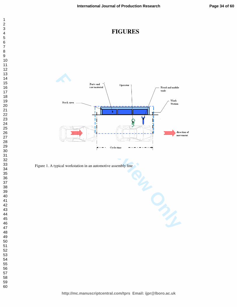
For Peer Review O
nly
FIGURES
Figure 1. A typical workstation in an automotive assembly line
Page 34 of 60
http://mc.manuscriptcentral.com/tprs Email: [email protected]
International Journal of Production Research
123456789101112131415161718192021222324252627282930313233343536373839404142434445464748495051525354555657585960

For Peer Review O
nly
Figure 2. Movements of an operator in his workspace
Direction of vehicles
Vehicle treated by a utility worker
Vehicle1
Vehicle2
Vehicle3
Vehicle4
Vehicle5
Min 0 Max Tcycl
e
Cycle time = length of workstation
Workspace of the operator
,i jDStart time
End time ,i jF
Workstation i and its workspace
Page 35 of 60
http://mc.manuscriptcentral.com/tprs Email: [email protected]
International Journal of Production Research
123456789101112131415161718192021222324252627282930313233343536373839404142434445464748495051525354555657585960

For Peer Review O
nly
Figure 3. Example of calculation of kcI
Page 36 of 60
http://mc.manuscriptcentral.com/tprs Email: [email protected]
International Journal of Production Research
123456789101112131415161718192021222324252627282930313233343536373839404142434445464748495051525354555657585960

For Peer Review O
nly
Figure 4. Representation of the workload of an operator at his workstation
Page 37 of 60
http://mc.manuscriptcentral.com/tprs Email: [email protected]
International Journal of Production Research
123456789101112131415161718192021222324252627282930313233343536373839404142434445464748495051525354555657585960

For Peer Review O
nly
Figure 5. Station constrained by a spacing constraint
Page 38 of 60
http://mc.manuscriptcentral.com/tprs Email: [email protected]
International Journal of Production Research
123456789101112131415161718192021222324252627282930313233343536373839404142434445464748495051525354555657585960

For Peer Review O
nly
Figure 6. Workstation over-constrained by a spacing constraint
Page 39 of 60
http://mc.manuscriptcentral.com/tprs Email: [email protected]
International Journal of Production Research
123456789101112131415161718192021222324252627282930313233343536373839404142434445464748495051525354555657585960

For Peer Review O
nly
Figure 7. Workstation under-constrained by a spacing constraint
Page 40 of 60
http://mc.manuscriptcentral.com/tprs Email: [email protected]
International Journal of Production Research
123456789101112131415161718192021222324252627282930313233343536373839404142434445464748495051525354555657585960

For Peer Review O
nly
Figure 8. Workstation impacted by a spacing constraint
Page 41 of 60
http://mc.manuscriptcentral.com/tprs Email: [email protected]
International Journal of Production Research
123456789101112131415161718192021222324252627282930313233343536373839404142434445464748495051525354555657585960

For Peer Review O
nly
Figure 9. Workstation not impacted by a spacing constraint
Page 42 of 60
http://mc.manuscriptcentral.com/tprs Email: [email protected]
International Journal of Production Research
123456789101112131415161718192021222324252627282930313233343536373839404142434445464748495051525354555657585960

For Peer Review O
nly
Impacted
Under-constrained
Over-constrained
Figure 10. Example of possible nuances in the relation
Page 43 of 60
http://mc.manuscriptcentral.com/tprs Email: [email protected]
International Journal of Production Research
123456789101112131415161718192021222324252627282930313233343536373839404142434445464748495051525354555657585960

For Peer Review O
nly
0
5
10
15
20
25
30
35
40
45
50
0,00 0,10 0,20 0,30 0,40 0,50 0,60 0,70 0,80 0,90 1,00
Impact factor
Nu
mb
er
of
inv
oca
tio
ns
Figure 11. The correlation between impact factor ,i kpI and the number of solicitations of utility workers
Page 44 of 60
http://mc.manuscriptcentral.com/tprs Email: [email protected]
International Journal of Production Research
123456789101112131415161718192021222324252627282930313233343536373839404142434445464748495051525354555657585960

For Peer Review O
nly
Figure 12. Example of simplification of the processing times of a station
Vehicles withlow workload
Vehicles withhigh workload
Cycle time
Time
Vehicles
infR
supR
supT
infT
Vehicles withlow workload
Vehicles withhigh workload
Cycle time
Time
Vehicles
infR
supR
supT
infT
Page 45 of 60
http://mc.manuscriptcentral.com/tprs Email: [email protected]
International Journal of Production Research
123456789101112131415161718192021222324252627282930313233343536373839404142434445464748495051525354555657585960

For Peer Review O
nly
0
100
200
300
400
500
600
700
800
900
0 1 2 3 4 5 6 7 8 9 10 11 12 13 14 15 16 17 18 19 20 21 22 23 24 25 26 27 28 29 30
Nb of constraints
co
un
t
0,0
0,1
0,2
0,3
0,4
0,5
0,6
0,7
0,8
0,9
1,0
Ip
No respects Emergencies Emergencies+No respects
Ip
Figure 13: Results for instance no. 9
Page 46 of 60
http://mc.manuscriptcentral.com/tprs Email: [email protected]
International Journal of Production Research
123456789101112131415161718192021222324252627282930313233343536373839404142434445464748495051525354555657585960
For Peer Review O
nly
0
60
120
180
240
300
360
420
480
540
600
660
720
0 1 2 3 4 5 6 7 8 9 10 11 12 13 14 15 16 17 18 19 20 21 22 23 24 25 26 27 28 29 30
number of constraints
co
un
t
0,0
0,1
0,2
0,3
0,4
0,5
0,6
0,7
0,8
0,9
1,0
Ip
Mean difference std devstd dev Mean Ip
Figure 14. Evolution of pI and the mean absolute difference between the observed and detected
emergencies.
Page 47 of 60
http://mc.manuscriptcentral.com/tprs Email: [email protected]
International Journal of Production Research
123456789101112131415161718192021222324252627282930313233343536373839404142434445464748495051525354555657585960

For Peer Review O
nly
0
50
100
150
200
250
300
350
1 2 3 4 5 6 7 8 9 10 11 12 13 14 15 16 17 18 19 20 21 22 23 24 25 26 27 28 29 30
Nb of constraints (= Nb of work stations)
No respects Emergencies Emergencies+No respects
Figure 15. Evolution of the emergency calls for 1=pI
Page 48 of 60
http://mc.manuscriptcentral.com/tprs Email: [email protected]
International Journal of Production Research
123456789101112131415161718192021222324252627282930313233343536373839404142434445464748495051525354555657585960

For Peer Review O
nly
0
200
400
600
800
1000
1200
0 1 2 3 4 5 6 7 8 9 10 11 12 13 14 15 16 17 18 19 20 21 22 23 24 25 26 27 28 29 30
Nb of constraints
co
un
t
0,0
0,1
0,2
0,3
0,4
0,5
0,6
0,7
0,8
0,9
1,0
Ip
No respects Emergencies Emergencies+No respects
Ip
Figure 16. Numerical experiments for two-temporization work stations
Page 49 of 60
http://mc.manuscriptcentral.com/tprs Email: [email protected]
International Journal of Production Research
123456789101112131415161718192021222324252627282930313233343536373839404142434445464748495051525354555657585960

For Peer Review O
nly
Station21 1,00
22 0,97
8 0,74
7 0,73
12 0,73
9 0,64
17 0,64
18 0,64
19 0,63
20 0,63
2 0,62
23 0,60
15 0,58
29 0,58
27 0,51
26 0,49
5 0,48
1 0,48
3 0,48
4 0,48
10 0,48
16 0,48
25 0,47
24 0,47
28 0,44
13 0,42
6 0,40
14 0,40
11 0,39
30 0,35
Global 0,57
0,00
0,10
0,20
0,30
0,40
0,50
0,60
0,70
0,80
0,90
1,00
21 22 8 7 12 9 17 18 19 20 2 23 15 29 27 26 5 1 3 4 10 16 25 24 28 13 6 14 11 30
ipI
Figure 17. Efficiency of the spacing constraints applied on the 23rd
May 2006 in Sevel Nord
Page 50 of 60
http://mc.manuscriptcentral.com/tprs Email: [email protected]
International Journal of Production Research
123456789101112131415161718192021222324252627282930313233343536373839404142434445464748495051525354555657585960

For Peer Review O
nly
Station1 1,00
2 1,00
3 1,00
4 1,00
6 1,00
8 1,00
9 1,00
10 1,00
16 1,00
17 1,00
18 1,00
22 1,00
23 1,00
27 1,00
28 1,00
29 1,00
5 1,00
24 0,99
25 0,98
7 0,98
12 0,98
21 0,91
14 0,91
15 0,90
20 0,89
19 0,87
11 0,87
13 0,86
26 0,84
30 0,82
Global 0,96
0,00
0,10
0,20
0,30
0,40
0,50
0,60
0,70
0,80
0,90
1,00
1 2 3 4 6 8 9 10 16 17 18 22 23 27 28 29 5 24 25 7 12 21 14 15 20 19 11 13 26 30
0,00
0,10
0,20
0,30
0,40
0,50
0,60
0,70
0,80
0,90
1,00
1 2 3 4 6 8 9 10 16 17 18 22 23 27 28 29 5 24 25 7 12 21 14 15 20 19 11 13 26 30
ipI
Figure 18. Efficiency of the selected constraints, for the production plan of 23rd
May.
Page 51 of 60
http://mc.manuscriptcentral.com/tprs Email: [email protected]
International Journal of Production Research
123456789101112131415161718192021222324252627282930313233343536373839404142434445464748495051525354555657585960

For Peer Review O
nly
Time Number of vehicles
0,07 5
1,04 39
1,09 471
1,52 121
1,53 7
1,69 2
1,91 74
Station 13
Time Number of vehicles
1,07 82
1,22 298
1,52 339
Station 6
Figure 19. Duration of tasks in stations 6 and 13
Page 52 of 60
http://mc.manuscriptcentral.com/tprs Email: [email protected]
International Journal of Production Research
123456789101112131415161718192021222324252627282930313233343536373839404142434445464748495051525354555657585960

For Peer Review O
nly
0
50
100
150
200
250
300
350
400
450
500
1 2 3 4 5 6 7 8 9 10 11 12 13 14 15 16 17 18 19 20 21 22 23 24 25 26 27 28 29 30
Nb of constraints
0,0000
0,1000
0,2000
0,3000
0,4000
0,5000
0,6000
0,7000
0,8000
0,9000
1,0000
No respects Emergencies Emergencies+No respects
Ip
Figure 20. Sensitivity analysis on the number of constraints.
Page 53 of 60
http://mc.manuscriptcentral.com/tprs Email: [email protected]
International Journal of Production Research
123456789101112131415161718192021222324252627282930313233343536373839404142434445464748495051525354555657585960

For Peer Review O
nly
0
50
100
150
200
250
300
350
400
450
500
1 2 3 4 5 6 7 8 9 10 11 12 13 14 15 16 17 18 19 20 21 22 23 24 25 26 27 28 29 30
Nb of constraints
0,0000
0,1000
0,2000
0,3000
0,4000
0,5000
0,6000
0,7000
0,8000
0,9000
1,0000
No respects Emergencies Emergencies+No respects
Ip
Figure 21. Analysis for the whole assembly line
Page 54 of 60
http://mc.manuscriptcentral.com/tprs Email: [email protected]
International Journal of Production Research
123456789101112131415161718192021222324252627282930313233343536373839404142434445464748495051525354555657585960

For Peer Review O
nly
- 1 -
LIST OF TABLE CAPTIONS
Table 1. Relationship between a workstation and a spacing constraint (SC)
Table 2. Data related to 30 workstations
Table 3. Spacing constraints applied the 23rd May 2006 in Sevel Nord
Table 4. Selected spacing constraints and their impact factors
Table 5. Synthesis of numerical results
Table 6. Zoom on stations number 6 and 13
TABLES
Table 1. Relationship between a workstation and a spacing constraint (SC)
Condition Relationship
k iVc Vp= Workstation is constrained by a SC
k i iVc Vp Vp=I and k iVc Vp− ≠ ∅ Workstation is over-constrained by a SC
i k kVp Vc Vc=I and i kVp Vc− ≠ ∅ Workstation is under-constrained by a SC
k iVc Vp ≠ ∅I , i k kVp Vc Vc≠I and k i iVc Vp Vp≠I Workstation is impacted by a SC
k iVc Vp = ∅I Workstation is not impacted by a SC
Page 55 of 60
http://mc.manuscriptcentral.com/tprs Email: [email protected]
International Journal of Production Research
123456789101112131415161718192021222324252627282930313233343536373839404142434445464748495051525354555657585960
For Peer Review O
nly
- 2 -
Table 2. Data related to 30 workstations
Optimistic case Average Case Pessimistic case
Station Min Max Tinf Tsup N/P Tinf Tsup N/P Tinf Tsup N/P
1 -0,7400 2,2200 0,6400 1,7400 5/7 1,0326 1,9875 2/5 1,0600 2,0500 2/5
2 -0,7400 2,2200 0,6180 1,6190 10/12 0,7493 1,6509 8/10 1,1790 1,6990 6/11
3 -0,7400 2,2200 0,8600 2,1800 2/5 0,8791 2,1800 2/5 0,8800 2,1800 2/5
4 -0,7400 2,2200 0,2800 1,6480 8/10 0,8856 1,8987 3/6 1,1190 1,9370 3/7
5 -0,7400 2,2200 0,4830 1,4920 123/125 1,2099 1,6283 9/14 1,2830 1,6820 7/15
6 0,0000 1,5300 1,0700 1,5200 1/2 1,1876 1,5200 1/2 1,2200 1,5200 1/2
7 -0,7400 2,2200 0,7000 1,4900 148/150 0,8096 1,6505 8/11 0,8100 1,6900 7/10
8 -0,7400 2,2200 0,6550 1,5280 30/32 0,7871 1,7022 6/8 0,7900 1,7380 5/7
9 -0,7400 2,2200 0,0000 1,6300 9/10 0,5406 2,0520 2/4 0,6000 2,2700 1/2
10 -0,7400 2,2200 0,2200 1,7400 5/7 0,6993 1,8888 3/5 1,0300 1,9500 3/7
11 -0,7400 2,2200 0,0000 1,6600 8/9 0,6693 2,2188 2/4 0,6900 2,3000 1/3
12 -0,7400 2,2200 0,6920 1,6260 10/12 0,8550 1,6494 8/11 0,9170 1,6660 7/10
13 0,0000 2,2200 0,0700 1,5200 18/19 1,0763 1,6634 4/6 1,0900 1,9100 1/3
14 -0,7400 2,2200 0,5500 1,7200 6/8 0,7852 2,0832 2/4 0,8300 2,1500 2/5
15 -0,7400 2,2200 0,6400 1,7100 6/8 0,6400 1,7680 5/7 0,6400 1,7900 4/6
16 -0,7400 2,2200 0,1800 2,4300 1/2 0,1800 2,7388 1/2 0,1800 2,7400 1/2
17 0,0000 3,1300 0,0000 1,6400 10/12 0,0000 2,7153 1/2 0,0000 2,9400 1/2
18 -0,7400 2,2200 0,0900 1,5000 74/76 0,0900 2,0582 2/3 0,0900 2,1800 2/4
19 -0,7400 2,2200 0,3400 1,5000 74/76 0,3690 1,7336 5/7 0,3700 1,8300 4/6
20 -0,7400 2,2200 0,4300 1,5000 74/76 0,4300 1,7573 5/7 0,4300 1,8500 4/6
21 -0,7400 2,2200 1,1500 1,6700 7/12 1,2775 1,6924 6/13 1,3800 1,7000 6/20
22 -0,7400 2,2200 1,1760 1,7210 6/11 1,3471 1,7210 6/17 1,4110 1,7210 6/27
23 -0,7400 2,2200 1,1450 1,5180 38/43 1,1461 1,6976 6/10 1,1480 1,8090 4/8
24 -0,7400 2,2200 0,7890 1,6270 10/13 1,0160 1,8110 4/7 1,0590 2,0670 2/5
25 -0,7400 2,2200 0,2700 1,7500 5/7 0,3558 1,9428 3/5 0,4800 2,1000 2/4
26 -0,7400 2,5200 0,6300 1,4900 178/181 0,9753 1,6738 9/13 1,1600 1,8000 5/10
27 -0,7400 2,2200 0,6200 1,4900 148/150 0,9292 1,7018 6/9 1,1450 1,7800 4/8
28 -0,7400 2,2200 1,0930 1,4870 211/215 1,0930 1,5255 32/36 1,0930 1,5570 19/23
29 0,0000 3,2570 0,8900 1,6300 11/14 1,3042 1,6300 11/21 1,4600 1,6300 11/94
30 -0,7400 2,2200 1,3500 1,5100 49/61 1,3922 1,5297 29/46 1,4600 1,5300 29/102
Page 56 of 60
http://mc.manuscriptcentral.com/tprs Email: [email protected]
International Journal of Production Research
123456789101112131415161718192021222324252627282930313233343536373839404142434445464748495051525354555657585960

For Peer Review O
nly
- 3 -
Table 3. Spacing constraints applied the 23rd May 2006 in Sevel Nord
DAD PLC ABR PB04 CMB TO FOND 3RG SIE BVA ESS
1 0,02 0,00 0,00 0,00 0,00 0,03 0,00 0,48 0,15 0,04 0,05
2 0,00 0,00 0,37 0,36 0,20 0,00 0,62 0,08 0,00 0,00 0,00
3 0,02 0,00 0,00 0,00 0,00 0,03 0,00 0,48 0,15 0,04 0,05
4 0,02 0,00 0,00 0,00 0,00 0,03 0,00 0,48 0,15 0,04 0,05
Criterion Ratio 5 0,02 0,00 0,00 0,00 0,00 0,03 0,00 0,48 0,15 0,04 0,05
DAD 1/4 6 0,13 0,17 0,03 0,05 0,02 0,02 0,04 0,40 0,12 0,03 0,04
PLC 1/4 7 0,10 0,18 0,39 0,43 0,22 0,00 0,73 0,06 0,00 0,00 0,00
ABR 2/6 8 0,10 0,18 0,40 0,41 0,20 0,00 0,74 0,06 0,00 0,00 0,00
PB04 1/2 9 0,02 0,03 0,07 0,13 0,17 0,02 0,00 0,64 0,12 0,03 0,04
CMB 1/4 10 0,02 0,00 0,00 0,00 0,00 0,03 0,00 0,48 0,15 0,04 0,05
TO 1/17 11 0,03 0,00 0,00 0,00 0,00 0,03 0,00 0,39 0,19 0,03 0,06
FOND 1/2 12 0,10 0,18 0,39 0,43 0,22 0,00 0,73 0,06 0,00 0,00 0,00
3RG 2/3 13 0,03 0,00 0,00 0,00 0,00 0,03 0,00 0,42 0,21 0,03 0,06
SIE 1/4 14 0,02 0,00 0,00 0,00 0,00 0,03 0,00 0,40 0,18 0,05 0,06
BVA 1/10 15 0,03 0,06 0,10 0,21 0,24 0,02 0,00 0,58 0,11 0,03 0,04
ESS 1/10 16 0,02 0,00 0,00 0,00 0,00 0,03 0,00 0,48 0,15 0,04 0,05
17 0,02 0,03 0,07 0,13 0,17 0,02 0,00 0,64 0,12 0,03 0,04
18 0,02 0,03 0,07 0,13 0,17 0,02 0,00 0,64 0,12 0,03 0,04
19 0,04 0,11 0,40 0,41 0,23 0,00 0,63 0,08 0,00 0,00 0,00
20 0,01 0,09 0,40 0,41 0,23 0,00 0,63 0,08 0,00 0,00 0,00
21 0,06 0,16 1,00 0,40 0,31 0,00 0,35 0,14 0,00 0,00 0,00
22 0,07 0,16 0,97 0,40 0,34 0,00 0,33 0,15 0,00 0,00 0,00
23 0,04 0,09 0,60 0,22 0,18 0,00 0,17 0,30 0,03 0,02 0,05
24 0,01 0,00 0,00 0,00 0,00 0,03 0,00 0,47 0,15 0,04 0,05
25 0,02 0,00 0,00 0,00 0,00 0,03 0,00 0,47 0,15 0,04 0,05
26 0,03 0,03 0,01 0,05 0,05 0,03 0,01 0,49 0,14 0,01 0,00
27 0,03 0,10 0,44 0,41 0,23 0,00 0,51 0,09 0,00 0,00 0,00
28 0,02 0,06 0,15 0,19 0,18 0,02 0,02 0,44 0,09 0,02 0,03
29 0,00 0,09 0,00 0,11 0,09 0,04 0,07 0,42 0,58 0,04 0,05
30 0,03 0,00 0,00 0,00 0,00 0,04 0,00 0,35 0,20 0,06 0,08
Page 57 of 60
http://mc.manuscriptcentral.com/tprs Email: [email protected]
International Journal of Production Research
123456789101112131415161718192021222324252627282930313233343536373839404142434445464748495051525354555657585960

For Peer Review O
nly
- 4 -
Table 4. Selected spacing constraints and their impact factors
1 3 2 23 29 28 17 6 27 22 8
1 1,00 1,00 0,00 0,25 0,19 0,54 0,85 0,86 0,00 0,00 0,002 0,00 0,00 1,00 0,24 0,03 0,07 0,03 0,00 0,72 0,33 0,753 1,00 1,00 0,00 0,25 0,19 0,54 0,85 0,86 0,00 0,00 0,004 1,00 1,00 0,00 0,25 0,19 0,54 0,85 0,86 0,00 0,00 0,00
Ratios 5 1,00 1,00 0,00 0,25 0,19 0,54 0,85 0,86 0,00 0,00 0,00
Constraint Optimistic Average Pessimistic 6 0,82 0,82 0,00 0,23 0,18 0,46 0,71 1,00 0,01 0,03 0,00
1 2/5 2/5 2/5 7 0,00 0,00 0,81 0,23 0,03 0,00 0,00 0,00 0,73 0,36 0,98
3 1/2 1/2 1/2 8 0,00 0,00 0,78 0,24 0,02 0,00 0,00 0,00 0,74 0,36 1,00
2 5/6 4/5 1/2 9 0,81 0,81 0,03 0,28 0,18 0,62 1,00 0,71 0,04 0,07 0,00
23 8/11 6/10 4/8 10 1,00 1,00 0,00 0,25 0,19 0,54 0,85 0,86 0,00 0,00 0,00
29 5/7 1/2 1/9 11 0,87 0,87 0,00 0,25 0,23 0,47 0,74 0,75 0,00 0,00 0,00
28 14/15 8/9 4/5 12 0,00 0,00 0,81 0,23 0,03 0,00 0,00 0,00 0,73 0,36 0,98
17 8/10 1/2 1/2 13 0,86 0,86 0,00 0,26 0,23 0,46 0,73 0,74 0,00 0,00 0,00
6 1/2 1/2 1/2 14 0,91 0,91 0,00 0,23 0,22 0,49 0,78 0,78 0,00 0,00 0,00
27 14/15 6/9 4/8 15 0,73 0,73 0,04 0,30 0,17 0,65 0,90 0,66 0,06 0,10 0,00
22 3/6 2/6 2/9 16 1,00 1,00 0,00 0,25 0,19 0,54 0,85 0,86 0,00 0,00 0,00
8 5/6 3/4 5/7 17 0,81 0,81 0,03 0,28 0,18 0,62 1,00 0,71 0,04 0,07 0,0018 0,81 0,81 0,03 0,28 0,18 0,62 1,00 0,71 0,04 0,07 0,0019 0,00 0,00 0,86 0,25 0,04 0,05 0,02 0,00 0,77 0,36 0,8720 0,00 0,00 0,89 0,25 0,04 0,06 0,02 0,00 0,77 0,36 0,8521 0,00 0,00 0,50 0,79 0,00 0,18 0,09 0,04 0,60 0,91 0,5222 0,00 0,00 0,49 0,77 0,00 0,17 0,10 0,04 0,58 1,00 0,5123 0,25 0,25 0,25 1,00 0,04 0,29 0,29 0,24 0,31 0,55 0,2424 0,99 0,99 0,00 0,26 0,19 0,53 0,84 0,85 0,00 0,00 0,0025 0,98 0,98 0,00 0,25 0,19 0,52 0,84 0,84 0,00 0,00 0,0026 0,84 0,84 0,02 0,21 0,23 0,53 0,78 0,75 0,00 0,01 0,0027 0,00 0,00 0,72 0,31 0,00 0,13 0,04 0,01 1,00 0,40 0,7228 0,57 0,57 0,08 0,31 0,14 1,00 0,69 0,51 0,14 0,13 0,0029 0,49 0,49 0,07 0,09 1,00 0,34 0,49 0,49 0,00 0,00 0,0530 0,82 0,82 0,00 0,04 0,26 0,44 0,70 0,70 0,00 0,00 0,00
Page 58 of 60
http://mc.manuscriptcentral.com/tprs Email: [email protected]
International Journal of Production Research
123456789101112131415161718192021222324252627282930313233343536373839404142434445464748495051525354555657585960

For Peer Review O
nly
- 5 -
Table 5. Synthesis of numerical results
Emergencies
+
No respects
counter 0 176 0
# of vehicles 0 100 0
# of workstations 11
Emergencies Emergencies Emergencies
+ + +
No respects No respects No respects
counter 46 113 30 113 84 79 195 66 64
# of vehicles 46 99 26 113 83 78 191 64 62
# of workstations 9 7 7
No respects Emergencies
Current
Optimistic
No respects Emergencies
Average
No respects Emergencies
Pessimistic
No respects Emergencies
Page 59 of 60
http://mc.manuscriptcentral.com/tprs Email: [email protected]
International Journal of Production Research
123456789101112131415161718192021222324252627282930313233343536373839404142434445464748495051525354555657585960

For Peer Review O
nly
- 6 -
Table 6. Zoom on stations number 6 and 13
Pessimistic
No respects Emergencies
emergencies
+
No respects
W. Station 13 59 0 0
W. Station 6 54 54 54
Page 60 of 60
http://mc.manuscriptcentral.com/tprs Email: [email protected]
International Journal of Production Research
123456789101112131415161718192021222324252627282930313233343536373839404142434445464748495051525354555657585960

![Quantifying evolutionary constraints on B-cell affinity ...vnminin.github.io/papers/McCoy2015.pdf · inference [16] for non-constant sequencing coverage and a star-tree phylogeny](https://img.pdfslide.us/doc/110x75/603248caf9d1c8573f7989d8/quantifying-evolutionary-constraints-on-b-cell-affinity-inference-16-for-non-constant.jpg)