Embed Size (px)
Citation preview


Feedback requested
• Overhead transparencies – keep or
convert to PowerPoint?
• Section handout
– Short outline
– Short outline with all visuals
– Expanded lecture notes

Sampling Design Basics
Objectives:
• Understand how attention to basic principals of
sampling design can improve the outcome of
monitoring projects.
• Identify: population, sampling unit, sample.
• List 3 types of non-sampling errors.
• Be able to calculate a 95% confidence interval
from actual sampling data.
• List 3 ways to increase the Power of a
monitoring study.

Topic OutlineA. Example of a failed monitoring project
B. Introduction to sampling
1. Definition of sampling
2. Why sample?
C.Key terms, important principals:
1. Populations and samples
2. Population parameters vs. sample statistics
3. Accuracy vs. Precision
4. Standard Error
5. Confidence Intervals
6. Finite vs. Infinite Populations
7. Sampling vs. nonsampling errors
8. False-change Errors, Missed-change Errors,
Power, and Minimum Detectable Changes

Topic Outline continued
Exercises
S1: Sampling a clumped population
S2: Identifying populations, sampling units, samples
S3: Calculating confidence intervals
S3.5: Power comparisons

Monitoring changes in Lomatium Cookii


Figure 1. Density of
Lomatium cookii in Macroplot
2 at the Agate Desert, 1989-
91. Bars represent 95%
confidence intervals.
Lomatium cookii were
counted in 50 1m2 plots each
year.

Figure 2. Frequency
histogram of number of
Lomatium cookii plants per
1m2 quadrant in macroplot 2
at the Agate Desert in 1989.
(n=50 quadrants; sum=156
plants; mean # plants/
quadrat=3.12; sd=11.17; 37
quadrats with no plants; 13
with plants; 3-1 plant, 2-2
plants, and 1 quadrat with
each of the following counts:
3, 4, 5, 13, 53, 59).
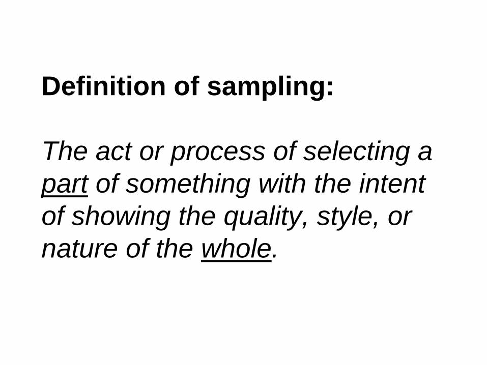
Definition of sampling:
The act or process of selecting a
part of something with the intent
of showing the quality, style, or
nature of the whole.
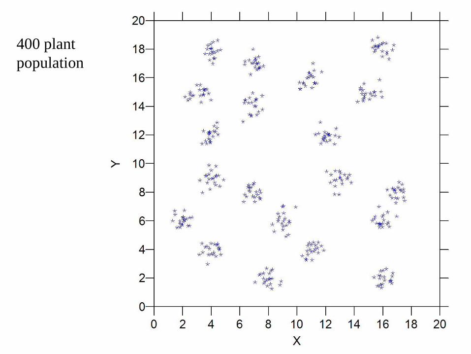
400 plant
population

A random
arrangement of
10 - 2m x 2m
quadrats
positioned within
a 400-plant
population.


A random
arrangement of
10 - 2m x 2m
quadrats
positioned within
a 400-plant
population.

Sample information
Coordinates
X Y
# of plants
2 2 4
6 4 0
16 4 3
12 6 2
14 6 5
6 8 10
0 12 0
Sample statistics (n=10)
Mean # plants/quadrat
x̄ = 5.0
Standard deviation:
s = 6.146
2 12 6
14 12 0
2 14 20
Population estimate
Est. pop. size = 500 plants
95% CI = ± 361 plants
Sample statistics for the 400-plant population.

Population
parameters
Tot. pop. size:
400 plants
Mean # plants /
quadrat (2m x 2m):
μ = 4
Standard deviation:
σ = 5.005

Sample information
Coordinates
X
Y
# of plants
2 2 4
6 4 0
Population parameters
Tot. pop. size: 400 plants
Mean # plants/quadrat:
μ = 4
Standard deviation:
σ = 5.005
16 4 3
12 6 2
14 6 5
6 8 10
0 12 0
Sample statistics (n=10)
Mean # plants/quadrat
x̄ = 5.0
Standard deviation:
s = 6.146
2 12 6
14 12 0
2 14 20
Population estimate
Est. pop. size = 500 plants
95% CI = ± 361 plants
Population parameters and sample statistics for the 400-plant population.
Accuracy is the closeness of a
measured or computed value to its
true value
Precision is the closeness of
repeated measurements of the
same quantity

An illustration of accuracy and precision in ecological
measurements. In each case, a series of repeated
measurements are taken on a single item, e.g. weight of a
single fish specimen. From Krebs, C.J. 1989. Ecological
Monitoring. Harper Collins, New York.

Sample with High Precision
9
10
14_
Mean = 11
Standard Deviation = 2.65
Sample with Low Precision
2
10
21_
Mean = 11
Standard Deviation = 9.54

Formula for standard error
n
sSE
Where:
s = sample standard deviation
n = sample size

Standard formula for a confidence interval
C.I. half-width = SE tvalue

Critical t-values for several levels of confidence
(for 2-sided confidence intervals).
degrees of freedom
80% 90% 95% 99%
1 3.078 6.314 12.706 63.656
2 1.886 2.920 4.303 9.925
3 1.638 2.353 3.182 5.841
4 1.533 2.132 2.776 4.604
5 1.476 2.015 2.571 4.032
6 1.440 1.943 2.447 3.707
7 1.415 1.895 2.365 3.499
8 1.397 1.860 2.306 3.355
9 1.383 1.833 2.262 3.250
10 1.372 1.812 2.228 3.169
11 1.363 1.796 2.201 3.106
12 1.356 1.782 2.179 3.055
13 1.350 1.771 2.160 3.012
14 1.345 1.761 2.145 2.977
15 1.341 1.753 2.131 2.947
16 1.337 1.746 2.120 2.921
17 1.333 1.740 2.110 2.898
18 1.330 1.734 2.101 2.878
19 1.328 1.729 2.093 2.861
20 1.325 1.725 2.086 2.845
21 1.323 1.721 2.080 2.831
22 1.321 1.717 2.074 2.819
23 1.319 1.714 2.069 2.807
24 1.318 1.711 2.064 2.797
25 1.316 1.708 2.060 2.787
26 1.315 1.706 2.056 2.779
27 1.314 1.703 2.052 2.771
28 1.313 1.701 2.048 2.763
29 1.311 1.699 2.045 2.756
30 1.310 1.697 2.042 2.750
35 1.306 1.690 2.030 2.724
40 1.303 1.684 2.021 2.704
45 1.301 1.679 2.014 2.690
50 1.299 1.676 2.009 2.678
100 1.290 1.660 1.984 2.626
200 1.286 1.653 1.972 2.601
500 1.283 1.648 1.965 2.586
= Infinity 1.282 1.645 1.960 2.576


Use the
Finite
Population
Correction
when
sampling
with
quadrats and
> 5% of all
possible
quadrats
n=10
N=100
10% of all
quadrats sampled

Finite
Population
Correction
“rewards”
you for
knowing
more about
the
population
n=98
N=100
98% of all
quadrats sampled

N
nNFPC
Formula for the finite population correction (FPC)
Where:
N = The total number of potential quadrat positions
n = The number of quadrats sampled

Example of calculating an FPC
•Total population area = 20m x 50m macroplot (1000 m2)
•Size of individual quadrat = 10 m2
•Sample size (n) = 30 quadrats
1002
m 10
2m 1000
N
N
nNFPC
100
3010083.0

Standard formula for a confidence interval
when sampling from a finite population
C.I. half-width = SE tvalue FPC

Non-Sampling Errors
• Biased selection rules
• Unrealistic or inappropriate techniques
• Sloppy field work
• Transcription and recording errors
• Inconsistent species identification

Sampling Errors
• The difference between a sample-based
estimate and the true population
• Errors resulting from chance – an
inevitable consequence of the sampling
process

Population estimate
Est. pop. size =
80 plants
95% CI = ± 119 plants
Sampling Error
Sample statistics
(n=10)
Mean = 0.8
plants / quadrat:
s = 1.75

Sampling Error
Population estimate
Est. pop. size =
960 plants
95% CI = ± 379 plants
Sample statistics
(n=10)
Mean = 9.6 plants
/ quadrat:
s = 5.58

Topic OutlineA. Example of a failed monitoring project
B. Introduction to sampling
1. Definition of sampling
2. Why sample?
C.Key terms, important principals:
1. Populations and samples
2. Population parameters vs. sample statistics
3. Accuracy vs. Precision
4. Standard Error
5. Confidence Intervals
6. Finite vs. Infinite Populations
7. Sampling vs. nonsampling errors
8. False-change Errors, Missed-change Errors,
Power, and Minimum Detectable Changes
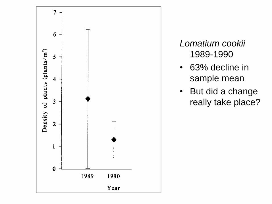
Lomatium cookii
1989-1990
• 63% decline in
sample mean
• But did a change
really take place?

No real change has taken place
There has been a real change
Monitoring system detects a change
Monitoring system detects no change
False-change
Error
(Type I ) α
No Error
(Power) 1-β
No Error
(1-α)
Missed-change
Error (Type II) β
Monitoring for change: possible errors

No real change has taken place
There has been a real change
Monitoring system detects a change
Monitoring system detects no change
False-change
Error
(Type I ) α
No Error
(Power) 1-β
No Error
(1-α)
Missed-change
Error (Type II) β
Monitoring for change: possible errors

The origin of the 0.05 “threshold”
• R.A. Fisher (1936)
– If P is between 0.1 and 0.9 there is certainly
no reason to suspect the hypothesis tested. If
it is below 0.02 it is strongly indicated that the
hypothesis fails to account for the whole of
the facts. We shall not often be astray if we
draw a conventional line at 0.05…

No real change has taken place
There has been a real change
Monitoring system detects a change
Monitoring system detects no change
False-change
Error
(Type I ) α
No Error
(Power) 1-β
No Error
(1-α)
Missed-change
Error (Type II) β
Monitoring for change: possible errors

Power = a function of (s, n, MDC, and α)
Standard
deviation
Sample
size
Minimum
detectable
change
False-change
(Type I) error
(1) Decrease
(2) Increase(3) Increase
(4) Increase
4 ways to improve Power


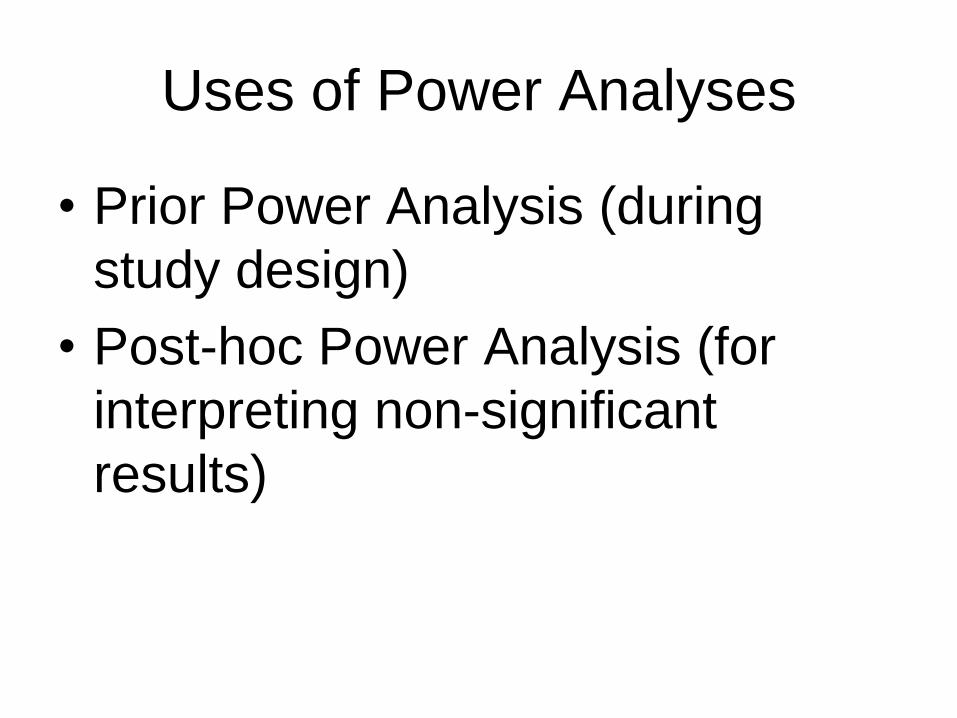
Uses of Power Analyses
• Prior Power Analysis (during
study design)
• Post-hoc Power Analysis (for
interpreting non-significant
results)

Power = a function of (s, n, MDC, and α)
Standard
deviation
Sample
size
Minimum
detectable
change
False-change
(Type I) error

n = a function of (s, Power, MDC, and α)
Standard
deviation
Sample
size
Minimum
detectable
change
False-change
(Type I) error

MDC = a function of (s, n, Power, and α)
Standard
deviation
Sample
size
Minimum
detectable
change
False-change
(Type I) error

Prior Power Analysis on 1989
Lomatium cookii data
• Minimum detectable effect size with and
= 0.10 = 200% change
• Power to detect a 50% change is only 0.18

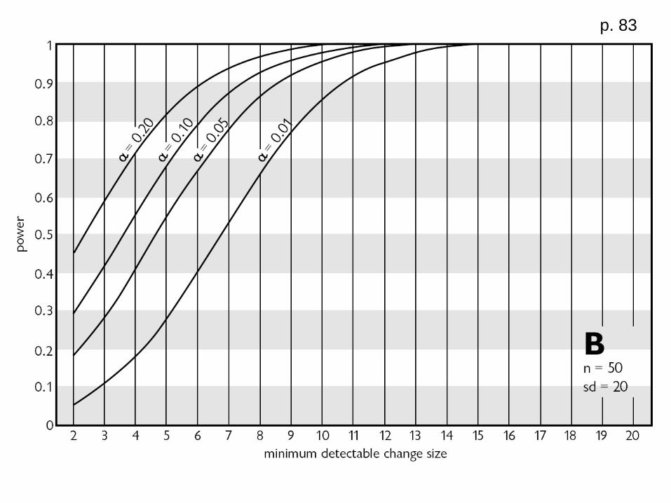
p. 83
Power = 0.17 when:
= 0.01 and MDC = 5
Power = 0.70 when:
= 0.20 and MDC = 5

p. 83
Power = 0.38 when:
= 0.05 and MDC = 5
Power = 0.86 when:
= 0.05 and MDC = 10
p. 83

p. 85

p. 85
Power in Figure
5.14a (p. 83)
n = 30, s = 20
MDC = 5 MDC = 10
= 0.01
= 0.05
= 0.10
= 0.20
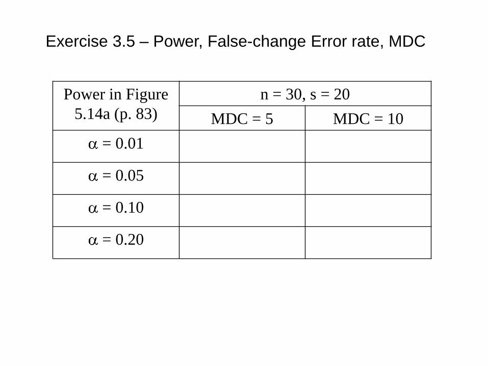
Exercise 3.5 – Power, False-change Error rate, MDC

Power in Figure 5.14a
(p. 83)
n = 30, s = 20
MDC = 5 MDC = 10
= 0.01 0.17 0.60
= 0.05 0.38 0.85
= 0.10 0.53 0.92
= 0.20 0.70 0.95
Power in Figure 5.14b
(p. 83)
n = 50, s = 20
MDC = 5 MDC = 10
= 0.01 0.28 0.86
= 0.05 0.55 0.95
= 0.10 0.67 0.97
= 0.20 0.83 0.99
Power in Figure 5.15b
(p. 85)
n = 30, s = 10
MDC = 5 MDC = 10
= 0.01 0.60 0.99
= 0.05 0.85 1.0
= 0.10 0.93 1.0
= 0.20 0.97 1.0

Sampling Design Basics
Objectives:
• Clearly state how attention to basic principals of sampling design can improve the outcome of monitoring projects.
• Clearly state the difference between a standard deviation and a standard error
• List 3 types of non-sampling errors.
• From a brief description of a monitoring study, identify the following components: population, sampling unit, sample.
• Be able to calculate a 95% confidence interval from actual sampling data.
• List 3 ways to increase the Power of a monitoring study.