The Definite Integral

The Riemann Integral

What is area? We are all familiar with determining the area of simple geometric figures such as rectangles and triangles.

However, how do we determine the area of a region R whose boundary may consist of non rectilinear curves, such as a parabola? To see how this could be done let us consider the following process.

Suppose that a function is continuous and non-negative on an interval . We wish to know what it means to compute the area of the region R bounded above by the curve below by the x-axis, and, on the sides, by the lines and , in short, the area under the curve as seen in the figure below.

We will obtain the area of the region R as the limit of a sum of areas of rectangles as follows: First, we divide the interval into

subintervals where . The intervals need not all be the same

length. Let the lengths of these intervals be respectively. This process divides the region R into strips (see the figure below).

2

Next, let's approximate each strip by a rectangle with height equal to the height of the curve at some arbitrary point in the

subinterval. That is, for the first subinterval select some contained in that subinterval and use as the height of the

first rectangle. The area of that rectangle is then

Similarly, for each remaining subinterval we will choose some and calculate the area of the

corresponding rectangle to be The approximate area of the region R is then the sum of these rectangular areas, denoted

by

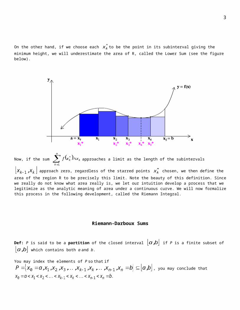
Depending on what points we select for the our estimate may be too large or too small. For example, if we choose each to be the point in its subinterval giving the maximum height, we will overestimate the area of R, called the Upper Sum (see the figure below).

On the other hand, if we choose each to be the point in its subinterval giving the minimum height, we will underestimate the area of R, called the Lower Sum (see the figure below).

3

Now, if the sum approaches a limit as the length of the subintervals approach zero, regardless of the

starred points chosen, we then define the area of the region R to be precisely this limit. Note the beauty of this definition. Since we really do not know what area really is, we let our intuition develop a process that we legitimize as the analytic meaning of area under a continuous curve. We will now formalize this process in the following development, called the Riemann Integral.

Riemann-Darboux Sums

Def: P is said to be a partition of the closed interval if P is a finite subset of which contains both a and b.

You may index the elements of P so that if , you may

conclude that

Def: Let be a partition of . We define

called the width of the subinterval

called the norm or mesh of the partition P.

Def: A partition is said to be a regular partition of if, for some , In this case,

Def: Let f be a function bounded on and a partition of .

By a Riemann sum of f over ¸ we mean the sum represented by 1 and defined by

any choice of ,

Remark: If on , then can be thought of as an approximation to the area under the curve of f from to

Def: Let f be a function bounded on . We say that f is Riemann integrable over if there exists a real number such

that for every partition and any

choice of , we have

2

1 Purcell writes for .2 The notation for the Riemann sum in this limit definition means that it does not matter what are chosen. We only require that

,

4

In this case, we say exists, write and denote by called the definite/Riemann

integral of f over .

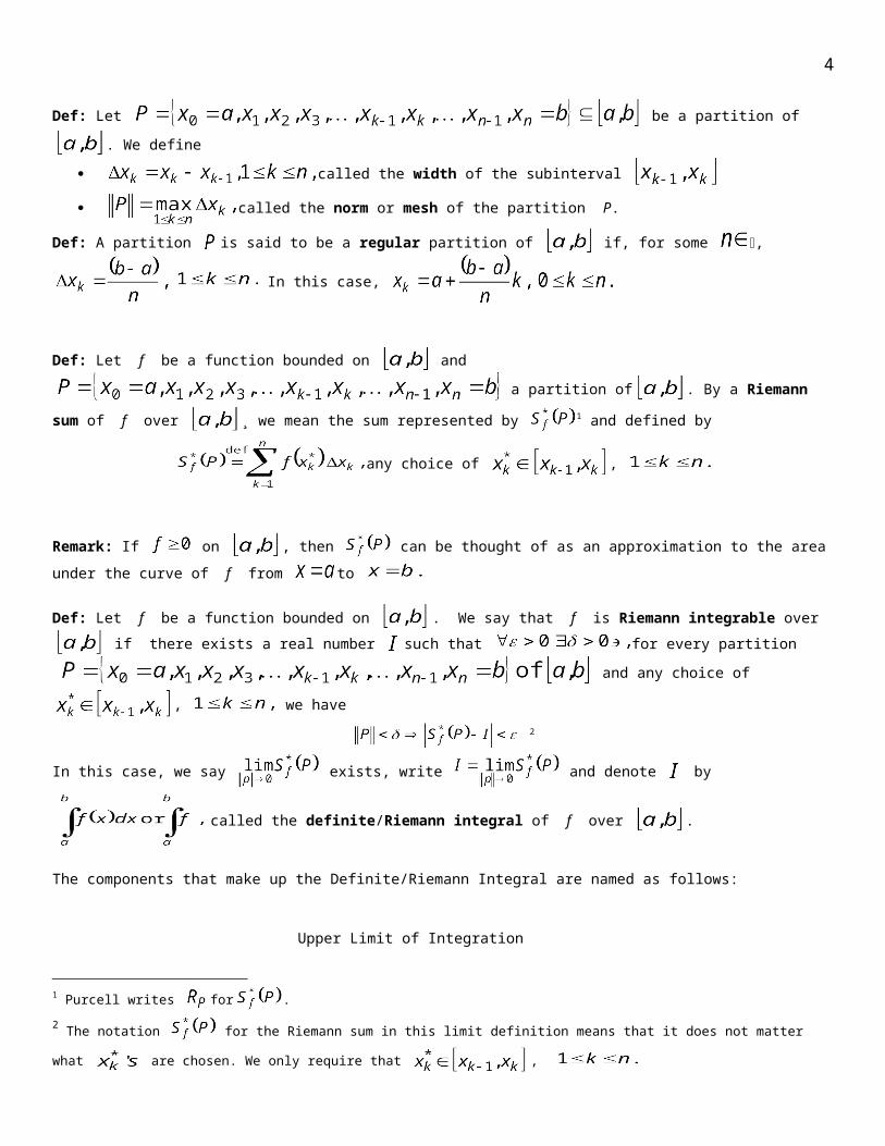
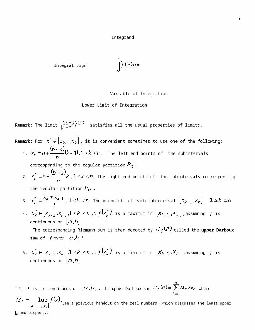
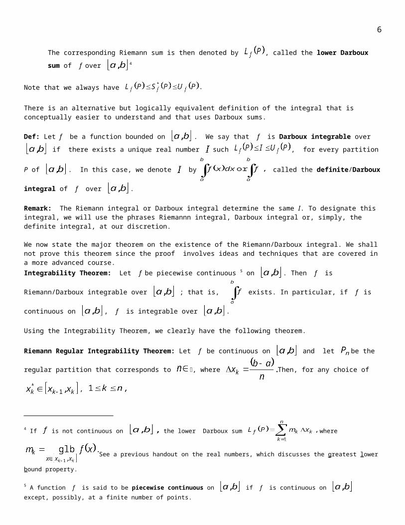
The components that make up the Definite/Riemann Integral are named as follows:

Upper Limit of Integration

Integrand

Integral Sign

Variable of Integration

Lower Limit of Integration

Remark: The limit satisfies all the usual properties of limits.

Remark: For , it is convenient sometimes to use one of the following:

1. . The left end points of the subintervals corresponding to the regular partition

2. The right end points of the subintervals corresponding the regular partition

3. The midpoints of each subinterval ,

4. is a maximum in assuming f is continuous on .

The corresponding Riemann sum is then denoted by called the upper Darboux sum of f over 3.

5. is a minimum in assuming f is continuous on .

The corresponding Riemann sum is then denoted by , called the lower Darboux sum of f over 4

Note that we always have

3 If is not continuous on the upper Darboux sum where See a previous handout

on the real numbers, which discusses the least upper bound property.

4 If is not continuous on the lower Darboux sum where See a previous handout on

the real numbers, which discusses the greatest lower bound property.

5

There is an alternative but logically equivalent definition of the integral that is conceptually easier to understand and that uses Darboux sums.

Def: Let f be a function bounded on . We say that f is Darboux integrable over if there exists a unique real number

such , for every partition P of . In this case, we denote by called the

definite/Darboux integral of f over .

Remark: The Riemann integral or Darboux integral determine the same I. To designate this integral, we will use the phrases Riemannn integral, Darboux integral or, simply, the definite integral, at our discretion.

We now state the major theorem on the existence of the Riemann/Darboux integral. We shall not prove this theorem since the proof involves ideas and techniques that are covered in a more advanced course.Integrability Theorem: Let f be piecewise continuous 5 on . Then f is Riemann/Darboux integrable over ; that is,

exists. In particular, if f is continuous on , f is integrable over .

Using the Integrability Theorem, we clearly have the following theorem.

Riemann Regular Integrability Theorem: Let f be continuous on and let be the regular partition that corresponds to

, where Then, for any choice of ,

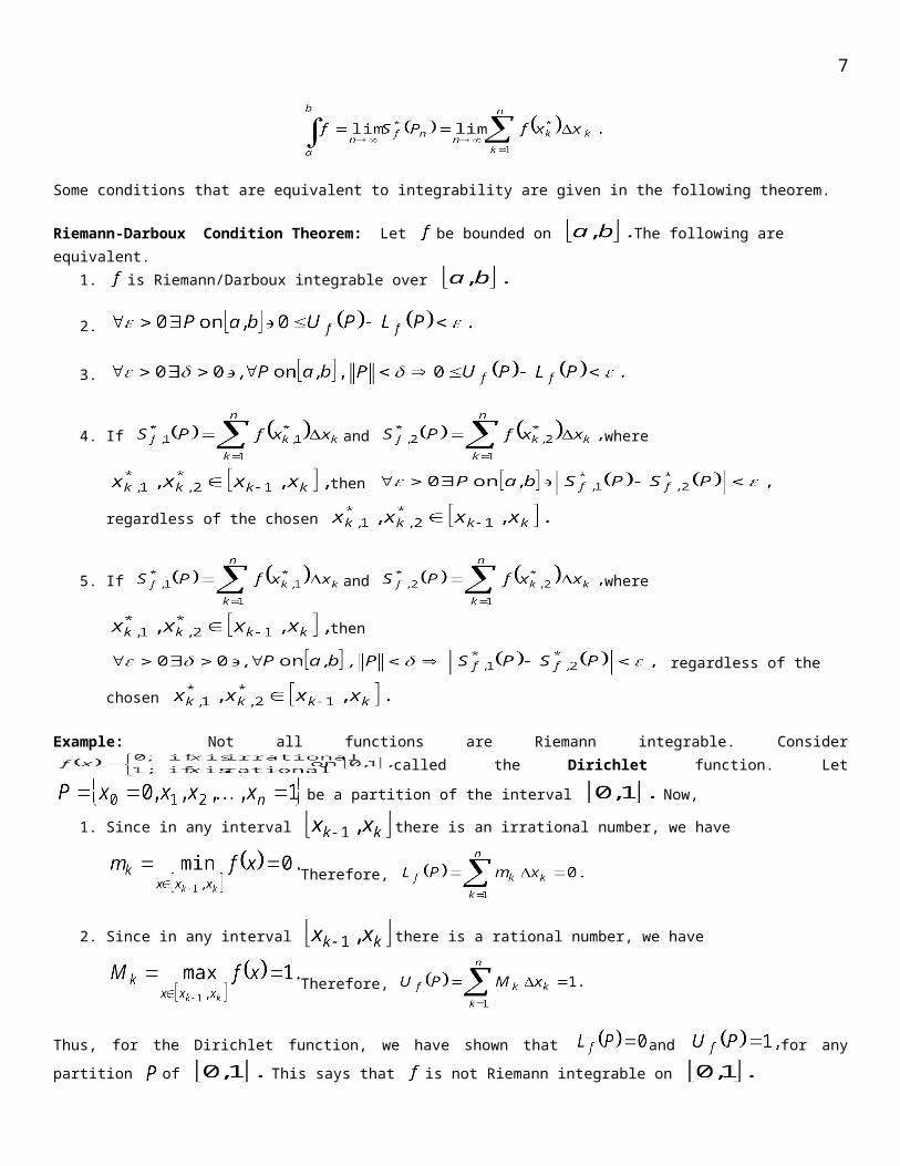
Some conditions that are equivalent to integrability are given in the following theorem.

Riemann-Darboux Condition Theorem: Let be bounded on The following are equivalent.1. is Riemann/Darboux integrable over

2.

3.

4. If and where then

regardless of the chosen

5. If and where then

regardless of the chosen

Example: Not all functions are Riemann integrable. Consider called the Dirichlet function.

Let be a partition of the interval Now,

5 A function f is said to be piecewise continuous on if f is continuous on except, possibly, at a finite number of points.

6

1. Since in any interval there is an irrational number, we have Therefore,

2. Since in any interval there is a rational number, we have Therefore,

Thus, for the Dirichlet function, we have shown that and for any partition of This says that is not Riemann integrable on

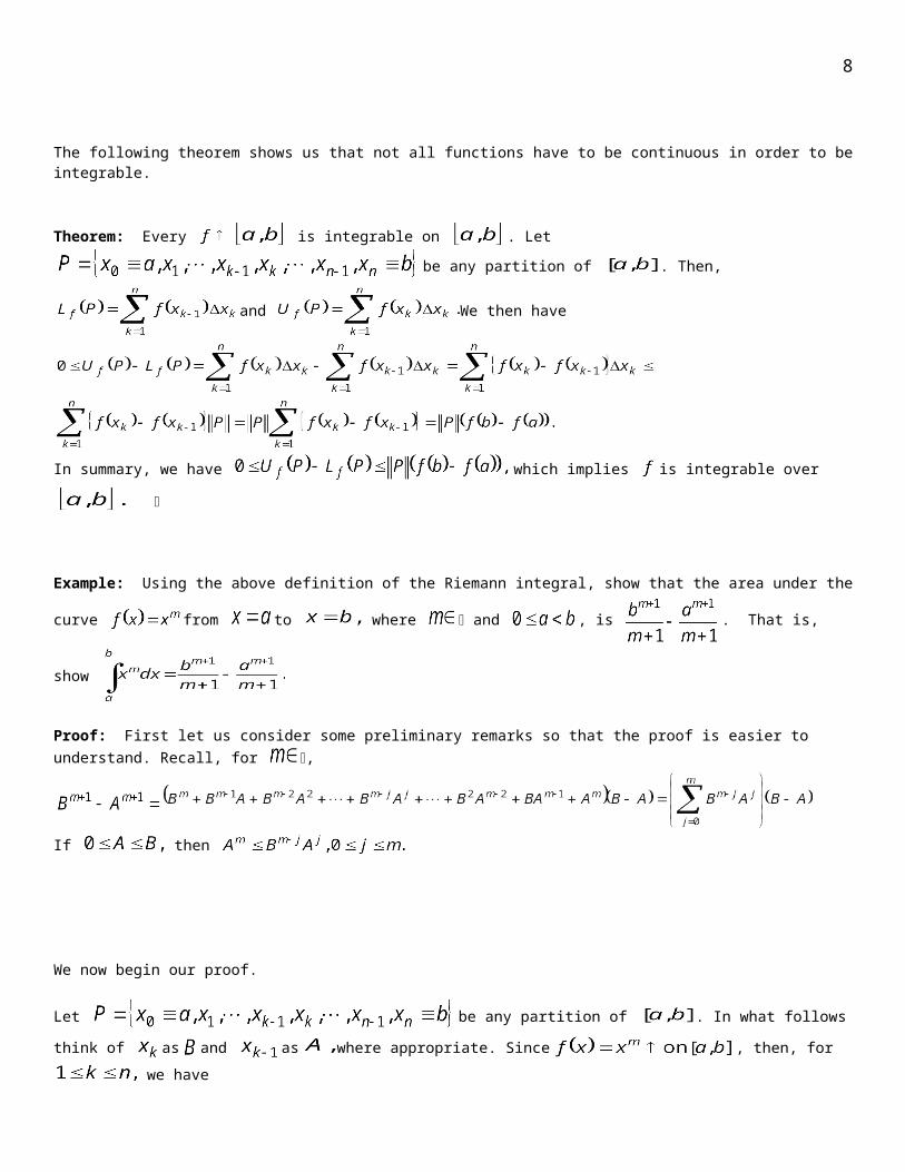
The following theorem shows us that not all functions have to be continuous in order to be integrable.

Theorem: Every is integrable on . Let be any partition of

. Then, and We then have

In summary, we have which implies is integrable over

Example: Using the above definition of the Riemann integral, show that the area under the curve from to

where and , is . That is, show

Proof: First let us consider some preliminary remarks so that the proof is easier to understand. Recall, for ,

If then

We now begin our proof.

Let be any partition of . In what follows think of as and as

where appropriate. Since , then, for we have

7

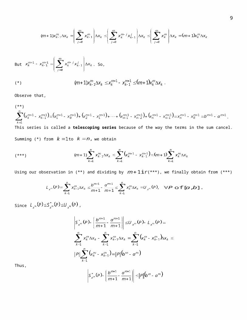
But . So,

(*) .

Observe that,

(**) .

This series is called a telescoping series because of the way the terms in the sum cancel.

Summing (*) from to we obtain

(***)

Using our observation in (**) and dividing by (***), we finally obtain from (***)

Since

Thus,

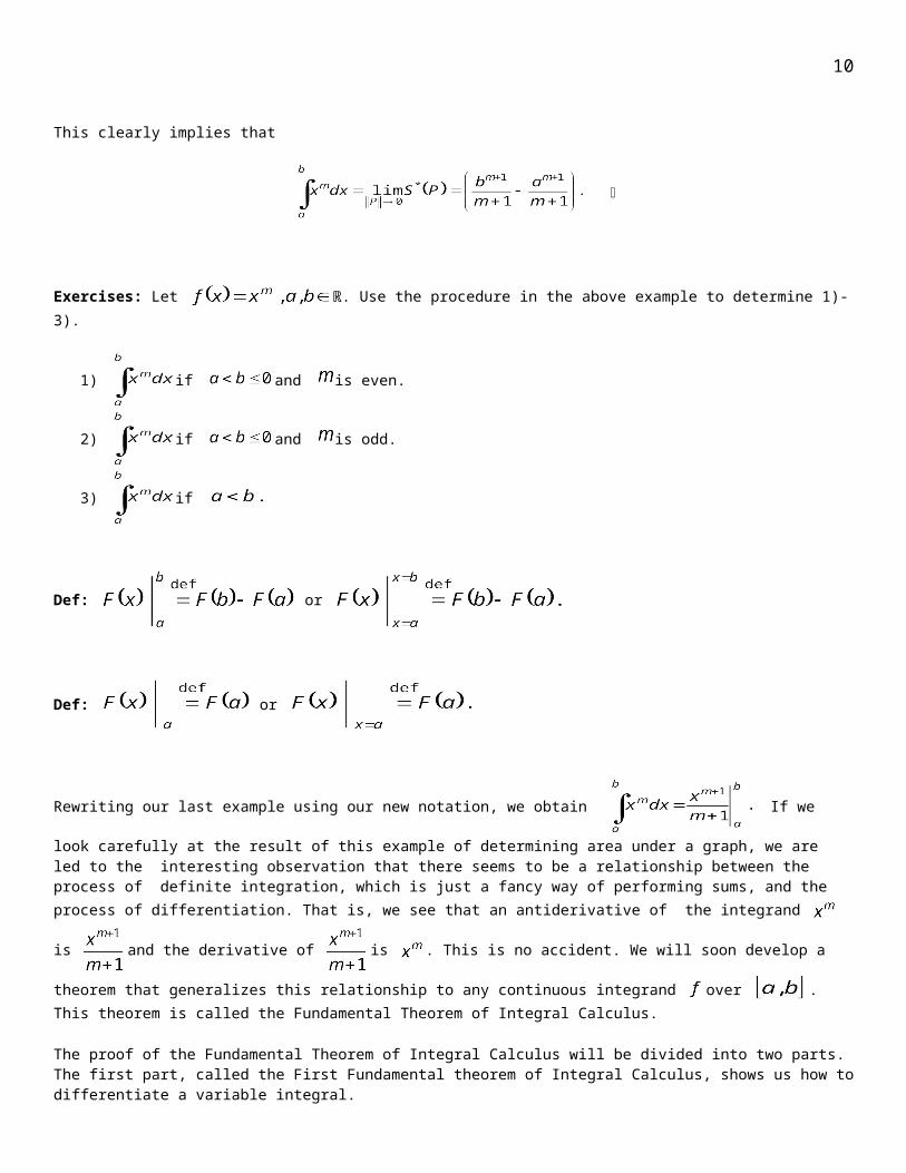
This clearly implies that

Exercises: Let ℝ. Use the procedure in the above example to determine 1)-3).

8

1) if and is even.

2) if and is odd.

3) if

Def: or

Def: or

Rewriting our last example using our new notation, we obtain If we look carefully at the result of this example

of determining area under a graph, we are led to the interesting observation that there seems to be a relationship between the process of definite integration, which is just a fancy way of performing sums, and the process of differentiation. That is, we see that an

antiderivative of the integrand is and the derivative of is . This is no accident. We will soon develop a theorem

that generalizes this relationship to any continuous integrand over . This theorem is called the Fundamental Theorem of Integral Calculus.

The proof of the Fundamental Theorem of Integral Calculus will be divided into two parts. The first part, called the First Fundamental theorem of Integral Calculus, shows us how to differentiate a variable integral.

The second part, called the Second Fundamental Theorem of Integral Calculus, shows us that one can compute the definite integral of a continous function by using any one of its antiderivatives. This part of the theorem has many practical applications, because it tremendously simplifies the computation of definite integrals.

The first published statement and proof of a restricted version of the Fundamental Theorem of Integral Calculus was given by James Gregory (1638–1675). Isaac Barrow (1630–1677) proved the first completely general version of this theorem. Barrow's student Sir Isaac Newton (1643–1727) completed the development of the surrounding mathematical theory, while Gottfried Leibniz (1646–1716) systematized the knowledge into a calculus involving infinitesimal quantities.

Lemma: Let ℝ. If a)b)

Proof of 1: By contradiction. Assume Then, Therefore, let By hypothesis, This is a contradiction.

Proof of 2: By hypothesis, by a).

9

Properties of the Riemann Integral

Let be continuous on an interval and Then,

1. Max-Min Rule.

Proof: Since given

a)

Also, b)

Combining a) and b), we obtain In summary, we have

Since was arbitrary, we have, by the above lemma applied to

and to , that

2. Boundedness Rule.

Proof:

3. Constant Rule.

4. Non-Negative Rule.

Proof: By the Max-Min Rule,

5. Positive Rule.

Proof: By the Max-Min Rule,

6. Sum Rule.

Proof: Let Given for all partitions we have that

10

a.

b.

c.

Let be a partition of such that and choose , the same for and

Note that . So, by a),b) and c), we obtain

Thus, Since was arbitrary, we conclude or

7. Scalar Multiple Rule.

Proof: Let and Given for all partitions of we have

a) .

b) .

Let be a partition of such that Note that . So, by a) and b), we obtain

Thus, Since was arbitrary, we conclude that or .

8. Linear Rule. This is equivalent to the Sum Rule together with the

Scalar Multiple Rule.

9. Non-Decreasing Rule.

Proof: by the Non-Negative Rule. By the Linear Rule, we then obtain

11

10. Increasing Rule.

Proof: by the Positive Rule. By the Linear Rule, we then obtain

11. Zero Width Interval Rule.

12. Order Integration Rule.

13. Additive Rule.

Proof: Since is continuous on , it is continuous on and on . Therefore,

a. of ,

b. of ,

c. of ,

Let and be a partitions of and , respectively, such that and Let . Then and . So,

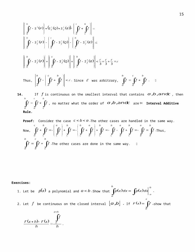
Thus, Since was arbitrary,

12

14. If is continuous on the smallest interval that contains , then , no matter what the order of

are Interval Additive Rule.

Proof: Consider the case The other cases are handled in the same way. Now,

Thus, The other

cases are done in the same way.

Exercises:

1. Let be a polynomial and Show that

2. Let be continuous on the closed interval If show that

Fundamental Theorem of Integral Calculus (FTIC)

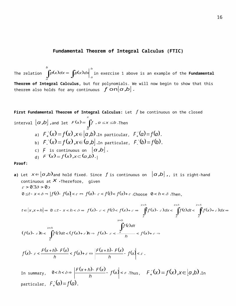
The relation in exercise 1 above is an example of the Fundamental Theorem of Integral Calculus, but

for polynomials. We will now begin to show that this theorem also holds for any continuous

First Fundamental Theorem of Integral Calculus: Let be continuous on the closed interval and let

Then

a) In particular,

b) In particular,

c) is continuous on d) |

Proof:

a) Let and hold fixed. Since is continuous on , it is right-hand continuous at Therefore, given

Choose Then,

13

In summary, Thus, In particular,

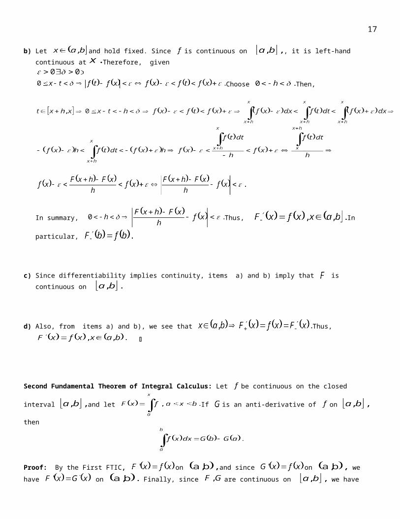
b) Let and hold fixed. Since is continuous on , it is left-hand continuous at Therefore, given

Choose Then,

In summary, Thus, In particular,

c) Since differentiability implies continuity, items a) and b) imply that is continuous on

d) Also, from items a) and b), we see that Thus,

Second Fundamental Theorem of Integral Calculus: Let be continuous on the closed interval and let

If is an anti-derivative of on then

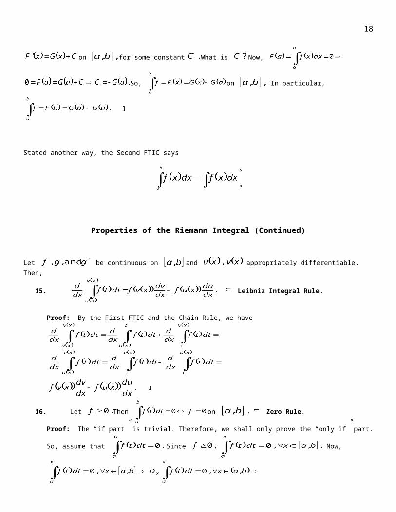
Proof: By the First FTIC, on and since on we have on Finally, since are continuous on we have on for some constant What is Now,

14

So, on In particular,

Stated another way, the Second FTIC says

Properties of the Riemann Integral (Continued)

Let be continuous on and appropriately differentiable. Then,

15. Leibniz Integral Rule.

Proof: By the First FTIC and the Chain Rule, we have

16. Let Then on Zero Rule.

Proof: The “if part” is trivial. Therefore, we shall only prove the “only if” part. So, assume that Since

Now,

by continuity.

17. U-Substitution Rule.

Proof: Let Then, Thus,

.

18. Change of Variable Rule.

15

Proof: Let Then,

19. where Here is said to be even. A Symmetry Law.

20. where Here is said to be odd. A Symmetry Law.

21. Absolute Value Rule.

Proof: Clearly, we have on By the Comparison Rule, we then have By the Comparison

Rule, we then have .

22. Definition of the average value of over

23. First Mean Value Theorem for Integrals (First MVTI).

Proof: The theorem is trivial if is constant on Therefore, we may assume that is not constant on By the

Max-Min Rule, we have that If then

This would then imply that on This contradicts the fact that is not

constant on Thus, In the same way, we also have Hence, Since

is continuous on by the Intermediate Value Theorem, there exists such that

24. where is periodic with period Periodic Rule for Integrals.

Proof: where we have used the change of variable

Applications of the Second FTIC

The Second FTIC can be restated in this way:

16

A function such as is called an accumulation function because it accumulates area under the graph of its derivatives for

Position as an Accumulation Function:

Exercise 1: An object moves along a coordinate line with velocity units per second. Its initial position at time is 2 units to the left of the origin.

a) Find the position of the object 3 seconds later.

b) Find the total distance traveled by the object during those 3 seconds.

Exercise 2: An object moves along a coordinate line with velocity units per second. Its initial position at time is 1 unit to the right of the origin.

a) Find the position of the object seconds later.

b) Find the total distance traveled by the object during those seconds.

Some Quantity as an Accumulation Function:

If measures the amount of some quantity at time , then the Second FTIC says that the accumulated rate of change from time to is equal to the net change in that quantity over the interval

Exercise 3: Water leaks out of a 55-gallon tank at the rate where is measured in hours and in gallons. Initially, the tank is full.

a) How much water leaks out of the tank between and hours?

b) How long does it take until there are just 5 gallons remaining in the tank?

Exercise 4: Water leaks out of a 200-gallon tank at the rate where is measured in hours and in gallons. Initially, the tank is full.

a) How much water leaks out of the tank between and hours?

b) How long does it take until the tank is drained completely?

Finding Area between TwoCurves

Slicing, Approximating and Integrating with Respect to the X-Axis

17

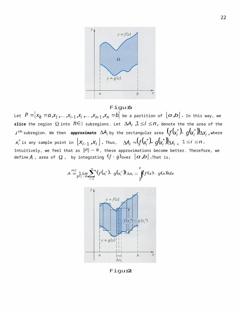
Consider two curves defined by the two functions continuous on the closed interval We want to compute the area of the region between these two curves from to .

Let be a partition of In this way, we slice the region into

subregions. Let denote the the area of the subregion. We then approximate by the rectangular area

where is any sample point in Thus, Intuitively, we

feel that as , these approximations become better. Therefore, we define , area of , by integrating over That is,

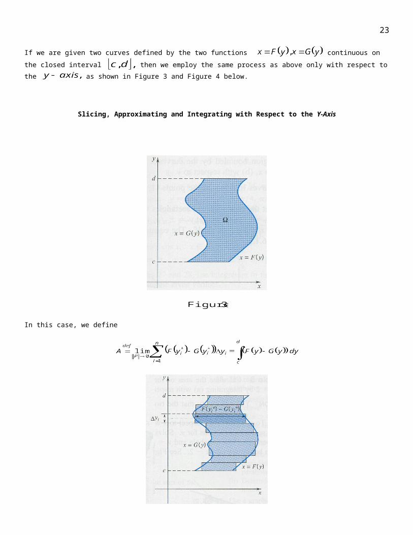
If we are given two curves defined by the two functions continuous on the closed interval then we employ the same process as above only with respect to the as shown in Figure 3 and Figure 4 below.

18

Slicing, Approximating and Integrating with Respect to the Y-Axis

In this case, we define

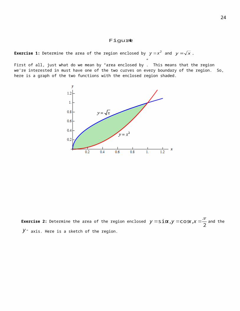
Exercise 1:  Determine the area of the region enclosed by and

First of all, just what do we mean by “area enclosed by”.  This means that the region we’re interested in must have one of the two curves on every boundary of the region.  So, here is a graph of the two functions with the enclosed region shaded.

19

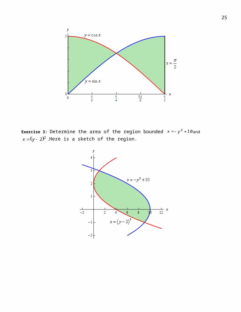
Exercise 2:  Determine the area of the region enclosed and the axis. Here is a sketch of the

region.

Exercise 3: Determine the area of the region bounded and Here is a sketch of the region.

20

Determining Volume

21

Volumes by Cross Sections

A cross section of a solid is a plane figure obtained by the intersection of that solid with a plane. The cross section of an object therefore represents an infinitesimal "slice" of a solid, and may be different depending on the orientation of the slicing plane. While the cross section of a sphere is always a disk, the cross section of a cube may be a square, hexagon, or other shape. Some other common cross sections are rectangles, triangles, semicircles, and trapezoids.

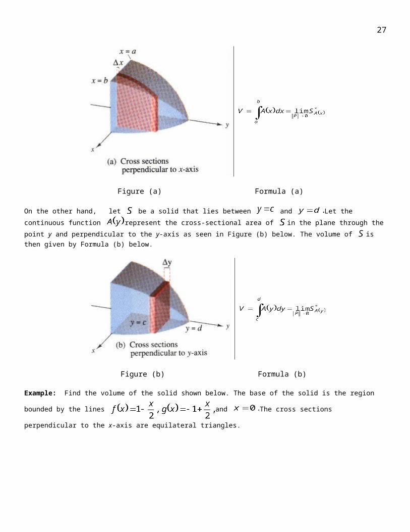
Integration allows us to calculate the volumes of such solids. That is, we may define the volume of a solid as a limit of a Riemann sum of cross sectional areas This is similar to the way we defined the area between two curves. Let be a solid that lies between

and Let the continuous function represent the cross-sectional area of in the plane through the point x and perpendicular to the x-axis, as seen in Figure (a) below. The volume of is then given by Formula (a) below.

Figure (a) Formula (a)

On the other hand, let be a solid that lies between and Let the continuous function represent the cross-sectional area of in the plane through the point y and perpendicular to the y-axis as seen in Figure (b) below. The volume of is then given by Formula (b) below.

Figure (b) Formula (b)

Example: Find the volume of the solid shown below. The base of the solid is the region bounded by the lines

and The cross sections perpendicular to the x-axis are equilateral triangles.

22

Solution: The base of each equilateral triangular cross section, area of each equilateral triangular cross section and corresponding volume element of the solid are

Base of Triangular Cross Section:

Cross Sectional Area of Equilateral Triangle:

Volume Element:

Because x ranges from 0 to 2, the volume of the solid is

Now that we have the definition of volume, the challenging part is to find the function of the area of a given cross section. This process is quite similar to finding the area between curves.

Solids of Revolution

Most volume problems that we will encounter will require us to calculate the volume of a solid of revolution. These are solids that are obtained when a plane region is rotated about some line. A typical volume problem would ask, "Find the volume of the solid generated by rotating the region bounded by the some curve(s) about some specified line." Since the region is rotated about a specific line, the solid obtained by this rotation will have a disk-shaped cross-section. We know from simple geometry that the area of a circle is given by For each cross-sectional disk, the radius is determined by the curves that bound the region. If we sketch the region bounded by the given curves, we can easily find a function to determine the radius of the cross-sectional disk at point x.

23

For example, the figures above illustrates this concept. The figure to the left shows the region bounded by the curve and the x-axis and the lines and . The figure in the center shows the 3-dimensional solid that is formed when the region from the first figure is rotated about the x-axis. The figure to the right shows a typical cross-sectional disk. A disk for a given value between 0 and 2 will have a radius of . The area of the disk is given by or equivalently, . Once we find the area function, we simply integrate from to to find the volume. In this example, the volume in question is given by

Variations on Volume Problems

There are two variations in problems of solids of revolution that we will consider. The first factor that can vary in this type of volume problem is the axis of rotation. What if the region from the figure above was rotated about the y-axis rather than the x-axis? We would end up with a different function for the radius of the cross-sectional disk. The function would be written with respect to rather than

, so we would have to integrate with respect to In general, we can use the following rule.

If the region bounded by the curves and the lines and is rotated about an axis parallel to the x-axis, write the integral with respect to x. If the axis of rotation is parallel to the y-axis, write the integral with respect to y.

The second factor that can vary in this type of volume problem is whether or not the axis of rotation is part of the region that is being rotated. In the first case, each cross section that is generated will be a disk while in the second case, each cross section that is generated will be washer shaped. This creates two separate styles of problems:

The Disk Method: The disk method is used when the cross sections are disk shaped. The radius of a cross section is determined by a single function, The area of the disk is given by the formula,

where The corresponding volume would then be The figure to the right

shows a typical cross-sectional disk.

24

The Washer Method: The washer method is used when the cross sections are washer shaped. The radius of a cross section is determined by a two functions, and This gives us two separate radii, an outer radius, from to the axis of rotation and

an inner radius from to the axis of rotation. The area of the washer is given by the formula, where

and The corresponding volume would then be

The figure to the left shows a typical cross-sectional washer.

Exercises:

1. Find the volume of the solid that is generated by revolving the region bounded by the curves and about the x-axis.

2. Find the volume of the solid that is generated by revolving the region bounded by the curves and about the y-axis.

3. Find the volume of the solid that is generated by revolving the region bounded by the curves and about t (a) the x-axis and about (b) the y-axis.

4. Find the volume of the solid that is generated by revolving the region bounded by the curves and about the x-axis.

5. Find the volume of a sphere of radius r.

6. Find the volume of a circular cone of radius r and height h.

7. The base of a solid is the region between the parabolas and Find the volume of the solid given that the cross sections perpendicular to the x-axis are squares.

8.  Find the volume of a pyramid whose base is a square with sides of length L and whose height is h (see the figure below).

Three and Two Dimensional Views of a Cross Section9. For a sphere of radius r find the volume of the cap of height h (see the figures below).

25

Three and Two Dimensional Views of a Cross Section

Two Dimensional View of a Cross Section

10. Find the volume of the solid whose base is a disk of radius r and whose cross-sections are equilateral triangles (see the figures below).

26

Three Dimensional Views of a Cross Section

Two Dimensional Views of a Cross Section

The axes of two equal cylinders of radius intersect perpendicularly. Find the volume common to the two cylinders.

27

Hint: First, the equations of the two cylinders are given by and In the figure below you see one eighth of the total volume in the first quadrant with a typical cross sectional area shaded. In fact, the cross sections are squares. To see this, from the figure we first note that the height of the rectangle is and the width is From the equations, we then obtain

Thus, our cross sections are squares.