Definition And Optimization Of The Drive Train Topology … Definition And Optimization Of The Drive Train Topology . For Electric Vehicles. Thomas Pesce. 1, ... The general approach

EVS26 International Battery, Hybrid and Fuel Cell Electric Vehicle Symposium 1

EVS26

Los Angeles, California, May 6-9, 2012

Definition And Optimization Of The Drive Train Topology

For Electric Vehicles

Thomas Pesce1, Markus Lienkamp

1Institute for Automotive Technology, Technische Universität München, Boltzmannstr. 15, 85748 Garching, Germany,

[email protected]

Abstract

Due to the limited range of battery electric vehicles, a low energy consumption is more desirable, than it is

in conventional vehicles. To accomplish this objective the paper focuses on an increased efficiency of the

drive train, its topologies and its components, as this is one of the most promising approaches. With a set of

basic characteristics of the desired vehicle (such as maximum speed, acceleration, climbing ability, class

and range) an optimal fitted drive train according to the energy consumption should be found. This includes

number, type and power of electric machines, transmission ratios, dynamic running radius, axle load

distribution and battery capacity. The general approach uses a method consisting of a developed

optimization routine and a specific simulation model.

The developed optimization algorithm reduces the value ranges or even the design parameters to minimize

the number of iterations. This intelligent algorithm is compared to conventional optimizers like pattern

search or genetic algorithms. For the vehicle model valid results are important. To ensure validity for all

possible topologies, vehicle and power classes an appropriate method is presented. Each relevant

component model and its respective scaling concept are validated. After validation of a vehicle model with

these component models, the scalability is transferable to the entire vehicle model. Some exemplary results

of the model are shown, such as the influence of axle load distribution, choice of high-energy or high-

power cells and potential of longitudinal torque-vectoring for multi-motor topologies.

Keywords: BEV (battery electric vehicle), powertrain, optimization, modeling, simulation

1 Introduction One of the biggest challenges of battery electric

vehicles (BEV) is the compensation of the

limited range, due to the small energy density of

state of the art accumulators. Although people

mostly use their cars for short distances up to

around 40 km, they simply would not accept

paying more for less than they would get out of a

conventional car.

One way to increase the range is to install a bigger

battery, which leads to increased costs and weight

and thus energy consumption. As the benefit of

this approach is not promising, the way to go is to

reduce the energy consumption of the vehicle. The

result is an increased range or a smaller battery

capacity with the opposite effect compared to

before, less costs and weight.

To achieve this goal there are two possible methods:

World Electric Vehicle Journal Vol. 5 - ISSN 2032-6653 - © 2012 WEVA Page 0024


Reduce all vehicle resistances

Increase the overall vehicle efficiency

The first option means a reduction of all vehicle

characteristics such as mass, cross-sectional area,

drag coefficient and rolling resistance coefficient.

All values are changeable in certain ranges, but

inevitably the vehicle will get smaller (seats,

payload), less safe (less crash zone, higher

accelerations) and/or less comfortable

(suspension, less auxiliary units). Some of these

disadvantages are compensated with the use of

new and better materials, but this raises the costs

significantly. If the value range is kept small

such that none of the mentioned disadvantages

appear the possible benefit in energy

consumption is negligible [1].

The second option takes the overall vehicle

efficiency into account. This comprises the

components of the drive train, as they are directly

involved in consuming energy and the

combination of this drive train with the car

around it. To get the lowest energy consumption

for a desired vehicle, the task is to find the

appropriate combination and dimensions of these

components. Considering all possibilities and

value ranges the solution space is very high.

However, to reach the goal adequate methods

like simulations and optimizations have to be

utilized.

One approach is presented in the following.

2 General approach

The challenge of the wanted method is to

calculate the result in an acceptable period of

time with an acceptable accuracy. To know for

what kind of basic vehicle the best drive train has

to be found a certain set of parameters is needed.

These are:

Vehicle class (for mass m, cross-sectional

area A, drag coefficient cw)

Payload mp

Maximum velocity vmax

Acceleration 0-100km/h a0-100

Gradeability (curb ramp, % at km/h) s

Range R

To define the most suitable drive train for this

set, first the design parameters, which have

relevance on the energy consumption (EC), have

to be assigned. These are:

Axle Load distribution alv

Type of electric motors mt

Number of electric motors mn

Position of electric motors mp

Transmission ratio(s) i

Dynamic running radius r

Battery cell type ct

With now knowing all input data and parameters a

method has to be found, which is able to manage

the large number of combinations as well as the

dependencies of the design parameters.

As the energy consumption is the target value it is

necessary to calculate it for a certain vehicle.

Simulations have been an adequate choice to do so

[2] and will also be the basis for the calculation

here. The modeling concept will be shown in detail

in chapter 3.

The size of the solution space requires a method to

avoid seeking the best topology manually.

Therefore different optimization algorithms exist

and have been used to find an optimal solution

automatically [3].

Summing all this up the whole method can be

described as shown in Figure 1.

Figure 1: General approach

The set of input parameters is used to calculate a

basic characteristic curve (see chapter 2.1).

Together with the basic vehicle data it serves as

the starting point for the optimization routine (see

chapter 2.2). This routine decides about the current

set of design parameters for the vehicle model.

After the simulation process the model returns the

associated energy consumption. Having found the

lowest energy consumption, the routine shows the

final result. In addition to the actual energy

consumption the result consists of the final values

of the afore-mentioned design parameters as well

as the mass and volume of the drive train

components (battery, power electronics, motor,

transmission).



2.1 Derivation of basic characteristic

curve

To get a proper design of the electric motor the

typical constant torque/constant power

characteristic has to fit the vehicle’s needs. For

that curve values like nominal torque/speed,

continuous power and maximum speed is

needed. To calculate these values, all necessary

data are given by the input parameters.

The continuous power is derived either from the

maximum velocity or the gradeability depending

on which requirement is higher. Therefore the

vehicle resistance equations are used with the

relevant values of the input parameters. The

maximum motor speed derives from the

maximum velocity. For all mentioned

calculations the dynamic running radius r is set

to 0.3m.

To obtain the nominal speed, additionally the

desired acceleration is used. The basic idea is

that the amount of power needed for the

acceleration sequence Pacc has to be provided by

the motor Pcon. This means mathematically

spoken, that the area/integral of both curves has

to be identical (see Figure 2).

Figure 2: Acceleration and peak motor curve

Setting up the equations and solving them for the

nominal speed vnp, the solution is:

(1)

(

)

(2)

(

(

) ) (3)

For the continuous power Pcon the value from the

calculation above is used and am is the medium

acceleration from 0-100km/h.

The calculated nominal speed is now defined as

the nominal speed at peak torque. The nominal torque is set to the half of the peak torque,

assuming that the peak torque is only used for

some seconds during high accelerations, such as 0-

100km/h. A ratio of two for peak torque to

nominal torque is a common value for three-phase

motors used in vehicle applications. With nominal

torque and continuous power, the nominal speed is

derived. The last check ensures that the ratio of

maximum speed to nominal speed does not exceed

a value of three [4]. If this is the case, the

continuous power is increased until the mentioned

ratio is reached. To get closer to the real-world

performance, drive train losses have to be

considered. The power and torque values

respectively are divided by 0.9, which is a rough

estimation at full load.

As a result the derived basic characteristic curve

can be seen as the characteristic of a single-motor

propulsion system with the transmission ratio 1,

which is able to guarantee the desired driving

performance.

2.2 Optimization routine

The optimization routine has the task to control the

whole process from choosing the design

parameters for the vehicle model to processing the

result of the simulation for the next iteration.

Although some well-known optimization

algorithms like genetic algorithms or pattern

search algorithms have been successfully used for

comparable vehicle optimization problems [5],

they all suffer from not being able to find the

global optimum of non-smooth and discontinuous

functions like in this case. To get better results,

especially with a higher chance of finding the

global optimum, a new routine has been developed

solving the described problem [6].

The approach uses the property of the target

function of not being chaotic and is divided in

three major steps (see Figure 3).

Figure 3: Approach of the optimization routine



In the first phase every design parameter is

analyzed separately with a rough value step size.

This results in a trend of the energy consumption,

like monotony or concentration of good values in

a certain value range. Because of being not

chaotic all parameters will keep its characteristic

even in combination. This information is used in

the second step to either eliminate irrelevant

parameters in case of a monotone behavior or to

reduce the value range to the areas with good

consumption values. In the last step a full-

factorial analysis of the remaining parameters

with reduced value ranges is done.

As shown in [6] the presented method always

finds a better optimum in less time than a pattern

search or genetic algorithm.

3 Concept of vehicle model The target value energy consumption is

calculated with a simulated vehicle model.

Different boundary conditions lead to some

requirements the model has to fulfill.

Communication with optimization routine

Stable and flexible handling of all possible

design parameter combinations

Objective basis for comparison

Relatively fast calculation

Validated models of all drive train topologies

The communication requirement is obvious as

model and optimization are exchanging data. The

model uses the design parameters to calculate the

energy consumption and the optimization needs

that value to determine the next set of

parameters.

The model has to be very robust towards

changing parameters of large scales. As the input

parameters theoretically have no boundaries the

model has to manage a large scope of vehicle

characteristics. For example there should be no

problem with a very small and light-weight car

with huge power or vice versa. Flexibility is

needed as topologies like front-, rear-, all-wheel

drives with and without transmission and more

are possible solutions. Because the whole process

is running automatically it is not possible to

change something in the model. Everything has

to be done once beforehand.

The optimization analyses and compares the

energy consumption of each set of design

parameters returned by the simulation. To get

comparable data the simulation has to calculate

the consumption on an objective basis. Hence

driving-cycles are used in the simulation. For one

whole optimization process the same driving-cycle

is used for every iteration step. The cycle may be

changed in a following optimization run with equal

input parameters to measure the influence of

different cycles on the topology. Of course the

simulation will return more realistic consumption

values by using customer driving-cycles than

synthetic cycles.

The simulation model is called in every iteration

step of the optimization. Having detailed models

for accurate results the simulation needs a certain

amount of time for the calculation. To keep the

duration for a whole optimization process in

moderate bounds, like some hours on common

personal computers, the number of iteration steps

as well as the simulation time should be as small as

possible. The absolute number of iteration steps is

dependent on the performance of the optimization

method, which is at a good level as described in

chapter 2.2. So additionally the design of the

simulation model should regard the calculation

time.

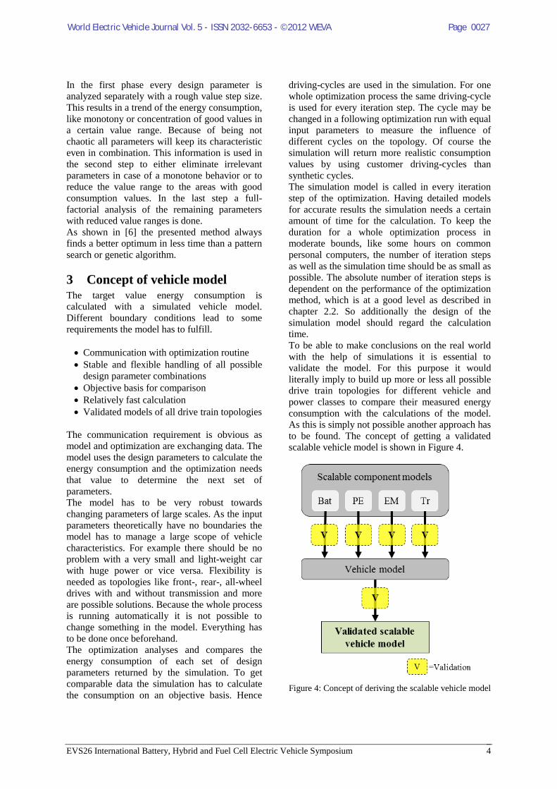
To be able to make conclusions on the real world

with the help of simulations it is essential to

validate the model. For this purpose it would

literally imply to build up more or less all possible

drive train topologies for different vehicle and

power classes to compare their measured energy

consumption with the calculations of the model.

As this is simply not possible another approach has

to be found. The concept of getting a validated

scalable vehicle model is shown in Figure 4.

Figure 4: Concept of deriving the scalable vehicle model



This method uses validated scalable component

models for the battery (Bat), power electronics

(PE), electric motor (EM) and transmission (Tr).

The single models build up the general vehicle

model. With the validation of the vehicle model

itself, conclusions on scaled vehicles are valid.

The component and the vehicle models are now

described in detail in the following chapters

together with the validation results.

3.1 Component models

For each relevant component the modeling

concept, the scalable values with its concept and

validation results will be presented.

3.1.1 Battery

The literature shows that battery models differ in

complexity and field of application. According to

[7] the different models can be classified as

follows:

Physical-chemical models

Equivalent circuit

Black-Box-Models

The complexity, effort for parameterization and

the needed data decrease from top to the bottom.

For the goal of this model the concept according

to the equivalent circuit seems to be an

acceptable trade-off between accuracy and

modeling effort.

Losses in batteries appear because of resistances

due to electrical effects, namely ohmic losses,

and electro-chemical effects, namely polarization

losses because of the passage and concentration

differences of the charge carriers. Considering

theses effects the equivalent circuit is shown in

Figure 5.

Figure 5: Equivalent circuit of battery model

The equation for the power losses compose of the

single loss-parts and that is:

(4)

Hence the current IKl affects the losses, which is

dependent on the operating point.

If all parameterization data are available the result

will have the best accuracy. As the electro-

chemical effects have a big relevance on mid- and

long-term analysis, the inner/ohmic resistance Ri influences the short-term behaviour. In this case at

least Ri has to be known to make conclusions on

battery losses in a driving cycle. For the presented

model data out of cell measurements are at hand

for a cylindrical high-energy and a pouch high-

power lithium-ion cell. Besides these

parameterization data the following values are

necessary to be able to specify the whole battery

pack.

Table 1: Parameters of battery model

Parameter Formula

symbol

Unit

Nominal capacity Cnom Ah

Nominal voltage Unom V

Max. discharge

current

Imax A

Cell mass mcell kg

Cell volume Vcell l

To calculate the number of cells (ncbat) of the

battery system together with cell mass (mbat) and

volume (Vbat) respectively the following equation

is used:

(5)

The battery has to be checked, whether it is

capable to manage the current of the maximum

vehicle power. If this is not the case the parallel

cell number has to be increased until the current of

each cell is smaller than the maximum discharge

current Imax. In either way the choice of high-

energy or high-power cells depends on the smaller

total number of cells ncbat.

Mass and volume of the battery pack is derived by

a multiplication with the given cell mass and

volume. Besides the actual cells a battery pack

consists of more components on system level.

These can be grouped in electric components,

battery management system (BMS), housing,

structural elements and parts for cooling. [8] states

values for the ratio of pack to cell mass and pack

to cell volume. Considering BEV the ratio for the

mass is 1.5 and for the volume 3.5.

The scalability of the battery model is described by

the combination of serial and parallel cells to adapt

the battery to different voltage, power and current

requirements. As the losses are calculated by using



an equivalent circuit for a single cell and the

pack consists of these cells, the scaled loss

calculation is also valid for the whole battery

pack. The validation of a single cell is ensured by

using real-world measurement data to

parameterize the model.

3.1.2 Power electronics

From an electric point of view the power

electronics has the function to conduct voltage

and current between battery and motor and to

transform direct current (DC) to alternating

current (AC) in driving mode and the other way

in recuperation mode. These functions cause the

occurring main losses in power electronics,

switching and conduction losses.

Common power electronics use a six-pulse

bridge inverter to transform DC to AC and a six-

pulse rectifier for the other way. The inverter

uses insulated gate bipolar transistors (IGBT) and

diodes as basic components and the rectifier only

needs diodes. To calculate the switching (sw) and

conduction (cond) losses of these elements the

derivation of [9] is used. Hence the equations for

the power electronics model are:

(

)

(

) (5)

(

)

(

) (6)

Where cos(φ) is the power factor and M the

modulation ratio between the battery voltage and

half of the intermediate circuit voltage.

The switching losses are described as:

( ) (7)

(8)

Here E is the energy loss, which is dependent on

voltage and current. For a scalable model this is

approximately linearized as follows:

(9)

The remaining parameters of the equations can

be extracted of data sheets. In sum Table 2 lists

all relevant parameters necessary for the used

power electronics model.

The overall power loss of an IGBT or diode is

the sum of conduction and switching losses. As

mentioned before the inverter has six IGBTs and

six diodes and the rectifier six diodes. Hence the

power loss in driving mode is the sum of IGBT and diode losses multiplied by six, whereas in

recuperation mode only the diode losses have to be

multiplied by six.

Table 2: Parameters of power electronics model

Parameter Formula

symbol

Unit

Collector-emittor voltage UCE V

Collector-emittor resistance rCE mΩ

Switch-on energy loss Eon mJ

Switch-off energy loss Eoff mJ

Current reference Iref A

Voltage reference Uref V

Voltage diode UD V

Resistance diode rD mΩ

Reverse recovery energy Err mJ

Switching frequency fs kHz

For the scaling of losses, mass and volume a set of

available data sheets of power electronic modules

are provided in a table. Dependent on the vehicle’s

power an appropriate module is chosen to get the

parameters for the model. To specify mass and

volume, empirical values for the whole power

electronics system like housing, assembly parts,

connectors and cooling are added to the data sheet

values.

To validate the power electronics model simulated

values are compared to manufacturer’s data.

Figure 6 shows the results exemplarily for the

inverter with a certain module.

Figure 6: Comparison of model and manufacturer values

An average deviation of 3.2W or 2.2% was

reached. For the rectifier the deviation is even less

than 1W or 0.5%.

3.1.3 Electric motor

The model of the electric motor has to give

information about its losses and its efficiency

respectively. It is possible to compile models for

the occurring losses, which are copper, iron and friction losses as well as additional empirical



losses. For example an advanced equivalent

circuit model of an electric motor would produce

such information [10]. Therefore a set of

parameters is needed like nominal speed, pole

count, resistances, inductivities, field flux linkage

or reactance. These values are sometimes

available in data sheets. For a continuous

scalability it is not sufficient to have efficiency

maps only for discrete motors of which these

parameters are available. The possibility of

directly scaling these parameters is not leading to

the preferred results. It is undetermined which

parameters have to be scaled correctly to cause

the desired effect and to keep a certain accuracy

and applicability to the real world. Trying to

derive these parameters by a rough dimensioning

process suffers from the same constraints. A

more detailed dimensioning to increase the

accuracy of the needed electro-magnetic

parameters is linked with a tremendous effort,

which would be an own topic [11]. Another well-

known scaling method are the laws of growth

[12]. They scale a motor geometrically and make

conclusions amongst others on torque and power

respectively, losses and efficiency respectively

and also mass and volume. But the method is

limited to smaller scaling ratios (<2), if a certain

accuracy is needed.

Here a scaling concept is presented, which offers

a sufficient accuracy and only requires efficiency

maps. Figure 7 shows the general approach of

this concept.

Figure 7: Motor scaling concept

With the set of efficiency maps a master map is

generated. Hence the natural upper bounds of

torque, speed and power in the master map are

prescribed by the single maps with the highest

value of these parameters. In consequence the

more maps are available the more universally valid

the master map gets. This conclusion is reinforced

by using efficiency maps of motors developed for

automotive applications.

With the desired characteristic (see chapter 2.1) the

efficiency values of the final map are a result of an

interpolation within the master map.

By using efficiency maps of actual motors this

scaling method validates itself. Every possible map

generated is in the mechanical, electro-magnetic

and thermal real-world bounds. This means a

generated map represents a motor, which would

possibly be developable.

An interpolation is also used to derive mass and

volume of the desired motor with the

specifications of the data sheets.

3.1.4 Transmission

To calculate the efficiency of a transmission, very

complex calculations are necessary and would

exceed the scope of this work. It is sufficient to

approximate the efficiency of a commonly used

helical geared gear-wheel for spur gears (SG) and

planetary gears (PG). The efficiency of a spur gear

is more or less constant and a common value is

97% [13]. In case of the planetary gear the

efficiency is dependent on the ratio, which is

described by the following equation:

(10)

As a spur gear can handle a gear ratio up to six in a

single step, higher ratios require a second step. The

ratio of the two steps is1 and is2 is given in [13] as:

⁄ (11)

(12)

The efficiency of the two-step spur gear is the

square of the single-step version.

The mass of these three transmission types (one-

and two-step spur gear, planetary gear) is

calculated with the volume of all involved gear-

wheels and an appropriate housing multiplied with

the corresponding density of the used materials. A

common material for gear-wheels is steel (ϱSt).

The small parts of other materials in alloys are

negligible. For the housing gray iron (ϱGG) is used.

The volume of the gear-wheels Vgw is calculated

according to DIN 3990, which uses the flank

bearing and root bearing to derive its dimensions.

The maximum torque Tmax and the desired

transmission ratio i is needed as input data. All the other necessary values in theses equations can be



extracted from the well-known literature for

transmissions, like [14].

The following equation shows the calculation for

the gear wheel mass mgw and is generally valid

for all three types:

(13)

For the housing simplified volume models are

used for scaling. Figure 8 shows the basic shapes.

Figure 8: Housing shapes for transmissions

The volume of the housing Vhous depends on the

size of the inner gear-wheels. Hence the mass of

the housing mhous is calculated as:

( ) (14)

The choice of the correct transmission type is

dependent on the target value. If the goal is

finding the smallest or lightest drive train the

decision for the best suited transmission type is

obvious. Mass and volume is calculated for all

three types and the smallest one is chosen. But if

the goal is getting the drive train with the lowest

energy consumption, lowest mass or best

efficiency might lead to an optimum.

Figure 9 shows the dependency of transmission

mass and efficiency on the energy consumption

for an exemplary vehicle in the New European

Driving Cycle (NEDC).

Figure 9: Influence of transmission mass and

efficiency on energy consumption

Additionally the slopes of the plane change for

different driving cycles. As a consequence once at

the beginning of the whole optimization process

this kind of diagram has to be calculated with the

rough vehicle characteristics and the chosen

driving cycle. The schema in Figure 10 shows the

whole resulting process of the transmission model.

Figure 10: Transmission model concept

3.2 Vehicle model

As mentioned in chapter 3 the vehicle model has to

be flexible and modular to manage all possible

drive train topologies, vehicle and power classes.

For that reason the model is split in two main

modules, one for the front and one for the rear

axle. Each group consists of the propulsion

components, which are electric motor,

transmission, brakes and wheels. Battery and

power electronics are not directly integrated in the

vehicle model. Their efficiencies are merged with

the efficiency map of the electric motor, which is

used in this model. The vehicle itself with

resistance equations, dynamic axle load

distribution etc. is modeled in another main

module. The energy consumption is calculated on

the basis of a driving cycle. A controller uses

actual and desired speed of the cycle to force the

actuating variables. To meet the model

requirements of guaranteeing a stable simulation

for each desired vehicle the controller parameters

have to be adapted. Empirical tests have shown

that the most important stability factor is the ratio

of vehicle mass and power. The maximum traction

force (adjusted by the transmission ratio) may not

exceed the transmittable force when slip is

considered. This is intercepted within the model

structure. For a traction to transmittable force ratio

smaller than 1 the amplification factor of the

controller is increased with the same ratio. Figure

11 shows the chart of the vehicle model.



Figure 11: Chart of the vehicle model

For the validation of the model a front-driven

electric vehicle with one electric machine and a

two-step transmission was available. The vehicle

parameters are listed in Table 3.

Table 3: Vehicle parameters

Parameter Formula

symbol

Unit Value

Mass m kg 1540

Drag resistance cw - 0.33

Wheel radius r m 0.305

Rolling resistance fr - 0.01

Cross-sectional

area

A m2 2.04

Wheelbase l m 2.47

Distance centre of

mass to front axle

lv m 1.13

Height centre of

mass

h m 0.4

Gear ratio i - 5.35

Nominal/peak

power

Pn/p kW 45/75

Nominal/peak

torque

Tn/p Nm 150/240

Battery capacity Csys kWh 12

As it was not possible to modify the vehicle with

the relevant measurement sensors to capture the

energy consumption, another method was used to

get the necessary value. A test drive with a fully

charged battery was done. The vehicle was

equipped with a GPS-logger to get the speed and

time correlation of the driven route (see Figure

12), which is needed for the basic data of the

reference driving cycle. After the test drive the

vehicle was recharged. The charged energy was

measured with a clamp meter. To consider only the

energy amount used for this drive, the losses of the

charger were eliminated by using the mean

efficiency of the manufacturer’s data.

Figure 12: Speed and time characteristic of driving cycle

Hence the energy consumption for this cycle was

20.9kWh/100km. To eliminate influences of the

recuperation strategy, the test drive was done

without recuperation, which was also applied to

the simulation.

The simulation calculates an energy consumption

of 19.6kWh/100km for the vehicle model.

Considering an unavoidable inaccuracy of the

involved component models as well as of the

measurement method a discrepancy of less than

7% is an acceptable result.

4 Longitudinal torque-vectoring If the topology has one motor at each axle the

torque is distributed according to their power ratio

in driving mode. For example if both motors have

the same power, both get the same amount of

torque, which is half of the whole desired torque.

In recuperation mode the torque is not actually

distributed, because the braking torque for each

axle is calculated according to the ideal brake

proportioning. This braking torque is covered by

the electric motor, if the torque is lower than the

motor’s peak torque. The exceeding torque is

supplied by the friction brake.

In the case of having a motor at both axles the

possibility appears to distribute the desired torque

between these two motors freely. In the model this

option can be activated for driving and

recuperation mode separately. The general set up

of the model is upgraded by an additional torque distribution module, which uses the desired torque



of the controller (see Figure 13). The

implemented algorithm distributes the torque

according to the lowest energy consumption for

driving and highest energy recovery for

recuperation respectively. Both cases consider

available peak torque and transmittable force,

when calculating the distribution.

Figure 13: Vehicle model with torque distribution

The gain and influence of the longitudinal

torque-vectoring is presented together with some

other results in the next chapter.

5 Results An interesting question to answer on the

component level is when to use high-energy or

high-power cells to get the smallest battery and

the fewest cells respectively. The determining

parameters are vehicle power and battery

capacity, which is dependent on the desired range

and vehicle.

Figure 14: High-energy vs. high-power cells

Figure 14 shows that there is one line separating the upper area, where high-power cells would be

the choice, from the lower area, where less high-

energy cells would be needed.

Another exemplary result is the influence of the

often unvalued parameter axle load distribution,

which is shown in Figure 15.

Figure 15: Influence of axle load distribution

The diagram shows the energy consumption of the

vehicle presented in chapter 3.2 for the driving

cycle of Figure 12 in dependency of the axle load

distribution for the original front drive and

additionally for the same vehicle and cycle but

with rear drive. The results show that the choice of

the axle load distribution can make a difference of

more than 1kwh/100km. If the topology with a

motor at each axle (each half of original motor

power) is added to this comparison and the ideal

brake proportioning is kept, the energy recovery is

of course higher and the influence of the axle load

distribution is almost gone.

Now the impact of the longitudinal torque-

vectoring is analysed. Again the vehicle and

driving cycle of chapter 3.2 is used with the motor

topology of the AWD configuration from above.

The diagram in Figure 16 shows a step by step

comparison between the energy consumption

without torque distribution and with distribution in

driving and recuperation mode.

Figure 16: Influence of torque distribution



Each mode only has a slightly benefit in energy

consumption up to a maximum of

0.5kwh/100km. A probable assumption of the

result for this vehicle, topology and driving cycle

combination is that the operation points of both

motors are already in good efficiency areas,

because of only having half of the power

compared to the single-motor configuration. On

the other hand this feature does not need

additional hardware and contributes to a smaller

energy consumption.

6 Conclusion The presented paper shows a method consisting

of an optimization routine and a vehicle model to

find the drive train with the lowest energy

consumption topology for a desired vehicle. The

optimization routine is used to automatically scan

the huge solution space to find an optimum. In

comparison to well-known conventional

optimizers, like pattern search and genetic

algorithms, the developed routine finds better

results in less time.

To get results that have relevance on the real

world it is essential to have a validated vehicle

model. Here the validation process includes even

the component models, as they have to be

scalable to be able to represent all possible

topologies, vehicle and power classes. Together

with the validation of a general vehicle model,

the validity of a scalable vehicle model is

ensured.

One exemplarily presented result is the influence

of the axle load distribution on the energy

consumption. Especially for front or rear drive

vehicles the influence of this parameter is

responsible for differences up to 1kWh/100km.

With an all-wheel drive topology having an

electric motor at each axle the energy

consumption decreases and the influence of the

axle load distribution is almost gone. This kind

of topology also has the possibility of a

longitudinal torque-vectoring, which is able to

reduce the energy consumption even more. For

the analyzed vehicle and topology the benefit of

torque distribution is present and hence reduces

the consumption a bit more.

The preliminary results promise a right approach

to the goal of finding the best drive train

topology of an electric vehicle when optimization

and simulation are fully integrated.

References [1] T. Haraguchi, Verbrauchsreduktion durch

verbesserte Fahrzeugeffizienz, ATZ, vol. 113,

no. 04, pp. 274–279, 2011

[2] S. Kerschl, Der Autarke Hybrid -

Optimierung des Antriebsstrangs hinsichtlich

Energieverbrauch und Bestimmung des

Einsparpotentials, Techn. Univ, Diss.--

München, 1998, ISBN°3-9806462-3-8,

München, FZG, 1998

[3] K. Kuchenbuch, et. Al,

Optimierungsalgorithmen für den Entwurf

von Elektrofahrzeugen, ATZ, vol. 113, no.

07-08, pp. 548–551, 2011

[4] A. Mathoy, Grundlagen für die Spezifikation

von E-Antrieben, MTZ, vol. 71, no. 09, pp.

556–563, 2010

[5] W. Gao, et. Al, Hybrid vehicle design using

global optimisation algorithms, IJEHV, vol.

1, no. 1, pp. 57–70, 2007

[6] T. Pesce, et. Al, Topologiedefinition für

Elektrofahrzeuge: Energetische Optimierung

der Antriebsstrangtopologie, Berechnung und

Erprobung bei alternativen Antrieben,

Gesamtfahrzeug - Energiespeicher -

Systemarchitekturen, Baden-Baden, 2011

[7] P. Keil, et. Al, Aufbau und Parametrierung

von Batteriemodellen, 19.

DESIGN&ELEKTRONIK-Entwicklerforum,

Batterien & Ladekonzepte, München, 2012

[8] C. Diegelmann, et. Al, Li-Ionen-

Akkumulatoren für Hybrid- und

Elektrofahrzeuge: Relation zwischen Zell-

und Systemeigenschaften, 2.

Automobiltechnisches Kolloquium,

Antriebstechnik, Fahrzeugtechnik,

Speichertechnik, Düsseldorf, VDI-

Wissensforum, pp. 1–12, 2011

[9] U. Probst, Leistungselektronik für Bachelors,

Grundlagen und praktische Anwendungen,

ISBN°9783446407848, München,

Fachbuchverl. Leipzig im Carl-Hanser-Verl,

2008

[10] E. Spring, Elektrische Maschinen, Eine

Einführung, ISBN°978-3-642-00884-9,

Berlin, Heidelberg, Springer-Verlag Berlin

Heidelberg, 2009

[11] W. Meyer, Automatisierter Entwurf

elektromechanischer Wandler, ISBN°978-3-

89791-406-3, München, Hieronymus, 2009

[12] K. Reichert, et. Al, Elektrische Antriebe

Elektrische Maschinen energie-optimal

auslegen und betreiben, Bern, Juni 1993

[13] G. Niemann, et. Al, Maschinenelemente,

Getriebe allgemein, Zahnradgetriebe -

Grundlagen, Stirnradgetriebe, ISBN°3-540-

11149-2, 2nd ed, Berlin [u.a.], Springer, 1983

[14] B. Künne, Einführung in die

Maschinenelemente, Gestaltung, Berechnung,



Konstruktion, ISBN°3-519-16335-7, 2nd

ed, Stuttgart [u.a.], Teubner, 2001

Authors

Thomas Pesce works at the institute

for automotive technology since May

2009 as scientific assistant in the field

of electric vehicle components. During

his study of mechanical engineering at

the Technische Universität München

he gained theoretical and practical

experience abroad and at local

automotive companies.

Prof. Dr.-Ing. Markus Lienkamp is

head of the institute for automotive

technology since 2009. After his study

and PhD at the University of

Darmstadt he joined VW, where he

hold different positions from vehicle

dynamics to department manager of

electronics and vehicle research in the

end.


Documents

Definition And Optimization Of The Drive Train Topology … Definition And Optimization Of The Drive Train Topology . For Electric Vehicles. Thomas Pesce. 1, ... The general approach