Embed Size (px)
Citation preview
DOCUMENTS DE TREBALL
DE LA DIVISIÓ DE CIÈNCIES JURÍDIQUES,
ECONÒMIQUES I SOCIALS
Col·lecció d’Economia
DEFICIT, HUMAN CAPITAL AND
ECONOMIC GROWTH DYNAMICS 1
Maria Carme Riera i Prunera 2
Adreça correspondència Anàlisi Quantitativa Regional, Research Group Departament d’Econometria, Estadística i Economia Espanyola Facultat de Ciències Econòmiques i Empresarials, Universitat de Barcelona Avda. Diagonal, 690 – 08034 Barcelona, Catalunya (Espanya) Tel.: 93 4037043 Fax: 93 4021821 e-mail: [email protected]
Recepció document : juliol 2003.
1 I am grateful for the comments and suggestions made by Theo Eicher, Stephen Turnovsky, Rafael Doménech, Luís Puch, Teresa Garcia -Milà, Marco Sanso and Enrique López-Bazo. 2 I am also indebted to the University of Washington for their kind hospitality

Abstract: Long-run economic growth arouses a great interest since it can shed light on the
income-path of an economy and try to explain the large differences in income we observe
across countries and over time. The neoclassical model has been followed by several
endogenous growth models which, contrarily to the former, seem to predict that economies
with similar preferences and technological level, do not necessarily tend to converge to
similar per capita income levels. This paper attempts to show a possible mechanism
through which macroeconomic disequilibria and inefficiencies, represented by budget
deficits, may hinder human capital accumulation and therefore economic growth. Using a
mixed education system, deficit is characterized as a bug agent which may end up sharply
reducing the resources devoted to education and training. The paper goes a step further
from the literature on deficit by introducing a rich dynamic analysis of the effects of a
deficit reduction on different economic aspects.
Following a simple growth model and allowing for slight changes in the law of human
capital accumulation, we reach a point where deficit might sharply reduce human capital
accumulation. On the other hand, a deficit reduction carried on for a long time, taking that
reduction as a more efficient management of the economy, may prove useful in inducing
endogenous growth. Empirical evidence for a sample of countries seems to support the
theoretical assumptions in the model: (1) evidence on an inverse relationship between
deficit and human capital accumulation, (2) presence of a strongly negative association
between the quantity of deficit in the economy and the rate of growth. They may prove a
certain role for budget deficit in economic growth.
Keywords: deficit, human capital accumulation, economic growth.
JEL classification: E62, H62, I22, O41

Resum: El creixement econòmic a llarg termini és un aspecte que ha desvetllat un gran
interès atès que pot facilitar el coneixement del camí seguit per la renda en una economia,
alhora que pot ajudar a explicar les grans diferències a nivell de renda que han existit i que
encara avui romanen entre els diversos països. El model neoclàssic fou seguit per diferents
models de creixement endogen que a diferència del primer semblen predir que les
economies amb preferències i un nivell tecnològic semblants no han de convergir
obligatòriament vers nivells de renda per càpita semblants. En aquest paper hem tractat de
mostrar un possible mecanisme a través del qual els desequilibris macroeconòmics i les
ineficiències, representats ambdós per la presència de dèficit, poden entorpir l’acumulació
de capital humà i per tant acabar entorpint també el creixement econòmic. Així, mitjançant
un sistema educatiu mixte, el dèficit és caracteritzat com un agent molest que pot acabar
exercint una important reducció dels recursos destinats a educació. L’article dóna un pas
més enllà de la literatura existent pel que fa a les qüestions sobre dèficit tot i introduint una
rica anàlisi dinàmica dels efectes d’una reducció deficitària en nombrosos aspectes
econòmics.
Partint d’un model de creixement simple i tot i afegint-hi certs canvis, especialment
concentrats en la llei d’acumulació de capital humà, s’aconsegueix arribar a un punt on el
dèficit redueix de manera important l’acumulació de capital humà. Per altra banda, una
reducció del dèficit continuada, entenent aquesta reducció com una direcció més eficient de
l’economia per part dels seus responsables, podria entendre’s com una manera de facilitar
el creixement. L’evidència empírica per una àmplia mostra de països sembla donar suport
als supostos teòrics del model: (1) evidència d’una relació inversa entre el dèficit i
l’acumulació de capital; (2) presència d’una forta associació negativa entre la quantitat de
dèficit en una economia i la taxa de creixement. Ambdós resultats semblen concedir un
paper destacat al dèficit en el procés de creixement econòmic.


1
1. Introduction
Deficits are an economic problem or may become so. Some questions we may wonder
about their origin can be posed as follows. Are they generated in response to demand
pressures from citizens? Alternatively, are they generated by interest groups that drive up
the size of government as pointed out by Buchanan, Rowley and Tollison (1987)?
Certainly, one of the main debates always has been the one about the size of the
government and the necessity or viability of a strong state. But, deficits lead to major
questions referring to the role of the government and how good/bad could be the creation of
oversized governments, questions which became one of the important concerns of the
major classical economists such as Adam Smith, David Ricardo, Thomas R. Malthus, or
John S. Mill, whose ideas formed the basis of the political economy (so called dismal
science by Carlyle). The classical model of macroeconomics is exclusively supply driven
and aggregate demand adjusts essentially via interest rate. Hence, an increase in
government purchases (or a decrease in taxes) would imply an increase in the interest rate,
which would decrease physical capital formation and/or consumption. They claim that
financing government expenditures issuing more bonds (creating deficit) would certainly
divert agents’ inve stment between capital and government claims, thus withdrawing
resources from industry and productive investments. Underlying this mechanism there is
the idea that private investment is more productive than public expenditures, sustained
mainly by Smith and Ricardo. This last one linked taxes and debt finance under what came
to be called, following Buchanan (1976), the Ricardian Equivalence Theorem. The opposite
traditional view mainly assumes people as being shortsighted or myopic. Hence, they
consider that current consumption does not move as much as Ricardians believe. Even
though Ricardo (1817) himself seems to doubt that people were rational and farsighted
enough, which turns out to be rather ironic.
Diamond’s (1965) paper was one of the first efforts to formally study the effects of budget
deficits in the context of neoclassical models. He argued that a permanent increase in the
ratio of domestically held debt to national income depresses the steady state capital-labor
ratio. At the beginning of the nineties, only Drazen (1978) had considered the consequences

2
of deficit on human capital, given that the vast majority of studies dealing with deficit had
mainly centered on physical capital. However, human capital may be an important aspect to
take into account given that, as it follows from Trostel (1995), recent research suggests that
human capital is the most important component of national wealth3, in line with Romer
(1989), Benhabib and Spiegel (1994) or Temple (1999a).
Moreover, the likely negative relationship between deficit and long-run growth may be
interpreted, according to Easterly and Rebelo (1993), considering a tax smoothing, which
would imply that large deficits would be associated with low growth periods. Most of the
literature on this topic turns to the possibility that large deficits may simply be an indicator
of a huge public debt, which, in turn, could imply the presence of larger taxes and less
public capital in the future.
In this paper, we will intend to analyze the effects that macroeconomic disequilibria,
represented by deficits, may have on the economy. More specifically, we will characterize
them as a bug agent that slows both human and physical capital accumulation and thus
economic growth. Our last goal will be to try to explain how the presence of
macroeconomic disequilibria may influence growth and be able to explain the existence of
different types of equilibria (ones with low levels of physical and human capital and high
levels of deficit; others, with higher capital levels and lower values for deficit). We will do
this within a framework where human capital accumulation depends positively on existing
human capital mainly following the formulation by Lucas (1988) and also taking into
account Azariadis and Drazen (1990).
Section 2 reviews the concept of deficit in the context of macroeconomics. First, we
analyze different empirical aspects, revising some of the main empirical studies and results
on the relation mainly between deficit and growth. Then, we introduce the concept of
human capital glimpsing a likely relationship between deficit and human capital
accumulation. Section 3 presents a model formalizing the analysis of the effects that
3 Davies and Whalley (1989) suggest that the stock of human capital is about three times as large as the stock of physical capital.

3
macroeconomic disequilibria, represented by deficits, may have on the economy. It covers
the equilibrium, the dynamics and the numerical analysis and discussion of the transitional
path. Section 4 undertakes an empirical study and gives statistical evidence supporting the
main proposition of the paper, that deficit may harm both human and physical capital
accumulation, thus slowing down economic growth. Finally, section 5 concludes and
discusses some possible extensions of the analysis presented before.
2. Deficits and macroeconomic analysis
2.1. Empirical aspects
There is an extensive literature dealing with deficit and its likely influence on an economy.
For instance, Barro (1974) showed that government debt is neutral when private
intergenerational transfers are positive and when the rate of growth is lower than the
interest rate. Later, Carmichael (1982) extended debt neutrality when the rate of growth is
greater than the interest rate suggesting as sources of non-neutrality of public debt
heterogeneous tastes and uncertainty. Besides, Drazen (1978) argued that when
intergenerational transfers take the form of investments in human capital, government
bonds might affect the equilibrium employment and increase welfare. Barro (1989) gives
some empirical evidence on the economic effects of budget deficits. He argues that deficits
mainly support the Ricardian viewpoint. Eisner and Pieper (1988), Boskin (1988), Hansson
and Stuart (1987), among others, emphasize the role of deficit in real economic activity and
its effects on wealth. On the other hand, Ihori (1988), Tanzi and Blejer (1988), Eisner
(1989), van der Ploeg and Alogoskoufis (1994), show evidence of the significance of the
impact that deficit financing has exerted on certain economies.
In addition, Easterly and Rebelo (1993) provide a wide review of the statistical relations
between different fiscal policy measures, the level of development of the economy and the
rate of growth. Their results confirm the fact that the presence of a high correlation between
most of the fiscal variables under study (different taxes and budget deficit) and initial
income makes it difficult to isolate the effects of fiscal policy in the context of Barro

4
regressions. The presence of this correlation leads them to study fiscal policy as being
endogenous in the sense of being related to certain characteristics of an economy such as its
level of development. Results show that deficit is one of the fiscal variables whose relation
with growth is more robust. They also confirmed one of the stylized facts of the literature,
which is that deficit was consistently correlated with economic growth and private
investment. Fischer (1993b) results are in the same line, showing a robust correlation
between deficit and growth. Hence, evidence seems to suggest that deficits exert some
influence on factor accumulation, which becomes stronger when the variable under analysis
is productivity growth.
During the nineties, the debate focused on how the persistence of big deficits during the last
decades in most industrialized countries may partly account for the high interest rates
observed during this period. The classics emphasized the negative effects of deficits on the
economy mainly through the interest rate adjustment that operated reducing investment and
capital accumulation. The link between interest rate and deficit may be relevant for
different aspects. It may fall upon the interdependence of fiscal and monetary policy; it may
introduce a feedback component that may influence the degree of sustainability of public
debt; it may become a key part in the mechanism of fiscal shocks transmission between
countries; or it may also affect the consumption decisions taken by different economic
agents. The controversy on budget deficits exerting a significant or, on the contrary, a
neutral effect on nominal and real interest rates has been subject to wide discussion in the
literature.
Plenty of empirical studies have given proven evidence of the impact deficits exerted on
interest rates (Tanzi and Lutz, 1985; Evans, 1985, 1987; Cebula, 1988, 1991; Cebula and
Hung, 1992; Ballabriga and Sebastián, 1993; Esteve and Tamarit, 1996, Doménech et al.,
2001). However, some others do not find a statistically significant relationship (Kormendi,
1983; Darrat, 1989).
The IS-LM model assumes that pressures exerted over interest rates reducing the effect of
what some authors have called the Keynesian multiplier are a consequence of public
spending increases that have not been financed by taxes. Except for the extreme case of a

5
perfectly elastic LM curve, the effect is caused by the competition between public and
private sector in capturing resources. Later extensions of the model, introducing variable
prices, include the possibility of spending levels above the full employment, which implies
inflationary pressures, as well as real money stock decreases. The upward pressures on
interest rates induced by deficit, according to Goisis (1989), are more likely to happen in
this context. He also asserts that both changes in interest rates as well as crowding out
effects are larger the higher the rigidity of the monetary policy, the closer the economy is
from full employment, and the more precise is the perception of inflation. The relationship
between deficit and interest rates has also been studied applying equilibrium dynamic
models with perfect markets (overlapping generations, Diamond, 1965 and Bowles et al.,
1989; or random decease date, Blanchard, 1985). Most of them show that changes in the
intertemporal structure of taxes influence real variables.
In a more empirical level, if potential disequilibrium between supply of funds and required
investment is large it should be easy to foresee a strong reaction of long-run interest rates
given that agents would anticipate the lack of funds. The main path through which this
mechanism would act would be the temporary structure of interest rates. Following the
model by Blanchard and Fischer (1989), the effect of deficits on short-run interest rates is
small at the beginning. However, and due to the fact that agents anticipate the increase in
the level of debt (additional deficit), the effect is larger in the anticipated future short-run
interest rates. Turnovsky (1989) reaches a similar result using a complete macroeconomic
model, assuming that agents maintain rational expectations. In this model, the behavior of
the temporary structure of interest rates depends on whether fiscal policies are permanent of
temporary as well as anticipated or not. Whenever fiscal policy is unanticipated, the most
significant result is the fact that a permanent fiscal expansion exerts a larger effect on
expected future long-run interest rates then on present short-run interest rates. This would
imply, by means of the temporary structure of interest rate, a larger increase in the present
long-run interest rate. On the other hand, an anticipated fiscal expansion is likely to
increase both short-run and long-run interest rates by the same quantity.

6
2.2. Human capital and deficit
According to macroeconomic theory, when there is a change in government spending it
affects the demand for the economy’s production of goods and services, altering the
national saving. Following Mankiw (1992), if one considers that output is initially fixed by
the factors of production, an increase in government spending must be offset by a decrease
in any other of the demand components. Then, assuming that the disposable income is
unchanged, consumption is also unchanged; hence, an increase in government purchases
that is not accompanied with a tax increase should be offset by a decrease in private
investment. Considering that private savings are unchanged, government borrowing
decreases national saving, thus leading to an increase in the equilibrium interest rate of the
economy given that government needs to capture investors’ resources in order for these to
absorb new debt issuance (crowding-out). Under this situation, capital stock would grow
slower than in a balanced one, hence reducing the capacity of an economy to produce goods
and services and so depressing the national income growth. These conditions, as we have
previously said, would probably translate into an upward pressure on interest rates in such a
way that long-run interest rates could pass on the effects of deficits to the real side of the
economy. This is so since private sector expenditure components are especially sensitive to
interest rates (i.e. house or plant building) and even more to long-run interest rate changes.
When reducing investment by increasing interest rates, deficits may not only depress
physical capital accumulation but also human capital accumulation. If we assume an
education system where people have to finance at least part of their own education, then,
there might be an important role for interest rates in human capital accumulation too, in the
sense that it would be more costly for people to ask for loans in order to be able to pay for
their education (i.e. Sánchez-Losada, 1998). Hence, the agents’ decision of how many
resources devoted to education would depend negatively on the cost of funding it. We
could think of this one as the value of the interest rate they would have to pay on the funds
borrowed to finance education, that is, the interest rate in the economy. Certainly, a higher
rate of interest would make investment in both human and physical capital more costly;
apart from this, it would reduce the present value of the returns on human capital
investment, that is, future wages. If the present cost to invest in human capital were too

7
high, given that (future) human capital cannot be used as a collateral, then agents would
probably reduce their optimal resource allocation to education, even if human capital is
most times seen as an embodiment of skills, being both a source of new knowledge as well
as a factor of production.
Over the 1970’s and the 1980’s, growth of public spending has generated large fiscal
deficits in both industrial and developing countries. In several economies, further
borrowing has no longer been a viable possibility, forcing the country to either decrease
non-interest public spending or to increase taxes. Nevertheless, spending reduction, in most
cases, has not followed efficiency considerations but political ones, resulting in a structure
of public expenditures less conducive to growth, further depressing the economy. On the
other hand, in low developed countries, increasing taxes is very difficult. Empirical
evidence shows that attempts to increase taxes have not proved very successful. What is
more, when fiscal authorities have been able to increase taxes they have induced large
distortions as well as a reduction in the growth potential of the country. An increase in
taxes reduces households’ income both directly through tax payments and indirectly
through deadweight losses due to distortions arisen by taxes. According to Trostel (1995),
if taxes are based on income, an increase in future tax rates decreases future net wage,
which can be seen as the return on current human capital investment, decreasing the
benefits of investing in human capital. Thus, investment in human capital would be
discouraged during a deficit.
3. Model with deficit
3.1. Putting down the model
We start assuming that government expenditures are financed either by taxes or deficit.
Hence, a change in deficit, taking taxes as constant, would be linked directly to a change in
government spending. Under this situation, in order to illustrate the difference that the
presence of different values of deficit can make in an economy we will simulate a change
from a high to a low value of deficit in a certain economy ceteris paribus.

8
In order to formalize this argument, we will use a simple model where households choose
their private consumption time path according to their preferences represented by the
following intertemporal isoelastic utility function:
( )( )0
1 tCG e dtςθ ρ
ς
∞−Π = ∫ 0;θ > 1≤<∞− ς ; ( ) 11 <+θς
(1)
where C denotes aggregate consumption, G denotes the government investment in public
goods other than education, ρ is the rate of time preference and the parameter θ measures
the impact of this public consumption on the agent’s welfare 4.
For simplicity, we will assume that the population growth rate is null. On the other hand,
firms operate combining physical and human capital. We will assume a Cobb-Douglas
function of the form:
( )[ ] GNHK aaaaF GNHlKAY −= 1 10 << ia ; i = K, H, G, N
(2)
The agents’ objective is to maximize their utility (1) subject to both the laws for physical
and human capital accumulation. The former one will be formalized as follows:
KEGCYK Kδ−−−−=•
(3)
where E5 is an education transfer from the government.
4 Following Turnovsky (2000a,b), the parameter ς is related to the intertemporal elasticity of substitution, s say by ( )ς−= 11s . 5 We have not introduced E in the utility function to avoid a duplication since the education transfer should be used to acquire education, which would likely translate into a higher level of future consumption.

9
The law for human capital accumulation is formalized as:
≡− HJ Hδ HEHXlaH HJEHXl δηηηη −=
•
0 1iη< < ; with , , ,i l X H E=
(4)
where aJ is the productivity of schooling (an efficiency parameter); H is the stock of human
capital already existing in the economy (human capital stock of parents); X are the private
expenditure agents make in education (it could be seen as a loan asked to the financial
sector), which would partly determine the quality of individual specific education;
individuals devote l part of their endowment of time to education; and Hδ is the
depreciation rate for human capital. All factors exhibit decreasing returns, but the learning
sector is subject to increasing returns to human capital, education transfer and education
expenditure. With the introduction of H, we are assuming that already existing human
capital positively determines the accumulation of future human capital (with decreasing
returns, though). We can interpret E as a proxy for the quality of public schools; all
individuals face the same quality coming from E, which is outside the control of one agent.
This is an argument in the learning technology that is consistent with Card and Krueger
(1992) and Glomm and Ravikumar (1992). Furthermore, with the incorporation of both X
and E, we are introducing a mixed system of education.
The analytical framework for the deficit follows that in Ihori (1988), which contains basic
principals from Diamond (1965) and Gale (1973) as well as an extension of the Samuelson
consumption loans model.
.' BYrBEGDdeficittotal y =−++== τ
.BYEGDdeficitprimary y =−+== τ
(5)
(6)
where B, is the quantity of government bonds existing in the economy, yτ is the income tax
rate and D is a measure of current fiscal imbalance (budget deficit).

10
Some authors have examined a variety of alternative measures of deficit, most of them
concluding that for the purpose of conducting macroeconomic analysis the deficit that
makes sense is the one that Sargent and Wallace (1994) propose, the primary deficit,
namely the total deficit excluding debt payments. According to this, and given its higher
simplicity, in our model we will use the primary deficit.
Following Turnovsky (2000b) 6, we will assume that the government sets its current gross
expenditures on education, E, and other public investments, G, as fixed fractions of output,
namely:
eYE =
gYG =
(7)
(8)
where g and e are fixed policy parameters. Using (7) and (8) and considering government
deficit, d, as a fraction of output, we may set the government budget constraint as follows:
[ ] [ ] degdYYeg =−+⇒=−+ ττ (9)
Plugging (8) into (2) and rearranging, we get:
( )[ ] ( ) NGHK aaaaF NgYHlKAY −= 1
( )[ ] G
N
G
HG
K
G
G
Ga
a
aa
aa
aa
aF NHlKgAY −−
−−− −= 1
111
11
1
( )[ ] NHK NHlKAY σσσ −= 1
where we have redefined:
( ) ( ) ( )1
11 ; 1 ; 1 ; 1
G
GG
aa
aF K K G H H G N N GA A g a a a a a aσ σ σ−−≡ ≡ − ≡ − ≡ −
(10)
6 This specification is equivalent to setting G/Y constant. It is adopted by Barro (1990), or Devereux and Love (1995), or Turnovsky (1997).
11
Individuals will take their decision of how much to invest in education depending on two
aspects, the additional wage they are going to get thanks to their stock of human capital, as
well as the cost to finance their investment in education (i.e. interest rate of the economy or
interest rate on bonds, R). Hence, agents will face a trade off between: (i) investing in
physical capital and get, KY
Kσ ; (ii) investing in bonds and get R ; and (iii) asking for a
loan in order to invest in human capital during the present period and get a higher salary
than unskilled or uneducated people in the future period once interest payments, RX, are
discounted, NH wRXw >− . In any case, we assume that agents take their decision in a
context of perfect capital markets. The value 0>−− RXww NH would represent the skill
premium, where Hw and Nw are the rewards to skilled and unskilled workers respectively.
Essentially , the total reward to skilled workers is the wage received by an unskilled worker
(rewarding the raw labour) plus the marginal product derived from skills of a worker
(rewarding the skills each educated worker has) in the final goods sector. We will define
the marginal product of skills (or human capital, H), as HYHσ , and the marginal product
of raw labor as NYNσ . In addition, defining the wage each skilled individual gets in per
hour terms, we are left with the following expression for skilled wage:
( ) ( )lNY
wlN
HHY
ww HNHNH −+=
−+=
111
σσ
with NY
w NN σ=
(11)
where the second term in the right hand side of the equality can be considered as the skill
premium and it comes from dividing the reward to the whole bunch of skills, YHσ , by the
number of skilled hours worked in the economy, ( )lN −1 .
We could represent the trade off in terms of some arbitrage conditions, which will take the
following form:

12
( )
KYR
RKRXlN
Y
K
H
σ
σ
=
=−−1
1
(12a)
(12b)
It says that the money privately invested in education, X, will end up depending positively
on the additional salary due to human capital as well as negatively on the interest rate value
of the economy.
When the returns to physical capital, represented by the nominal interest rate in the
economy, are greater than the returns to human capital, agents will decide not to invest at
all in human capital, thus devoting no resources to studying. We will refer to any
equilibrium that satisfies this condition as an underdevelopment trap. Thus, in an economy
with no human capital accumulation, even if it accumulates physical capital, output is not
likely to grow. On the contrary, when returns to physical capital are equal to returns to
human capital, we reach an interior equilibrium as detailed below.
Taking this into account, we can rewrite the law for physical capital, (3) as:
KEGCYRXK Kδ−−−−=+•
(3’)
Performing the optimization by using a discounted Hamiltonian with costate variables m
for physical capital and q for human capital we obtain:
( )( ) ( ) ( )
−−
+
−−−−−−−+=ℑ
•
•
−
−−∞
∫
HHEHlXaqe
KRXKCNHlAKdmeeCG
HHt
Kytt
EHlX
NHHK
δ
δτς
ηηηηρ
σσσσρρςθ 1110
(13)
and taking into account (9), it yields the following first order conditions:
mGCC
=⇒=∂∂ℑ − θςς 10
(14a)

13
( ) ( ) ( ) 01
11 1 =
−
−+−−−−=∂∂ℑ −
llEHlXaqlNHAKdm
lHEl
HyHEHlXNNHK
σηητσ ηηηησσσσ
( )( ) ( )lYd
llJ
qm
yH
HEl
−−−
−
−=⇒
111
τσ
σηη
with J as defined in (4)
RXJ
qm
XXη
=⇒=∂∂ℑ
0
(14b)
(14b’)
(14c)
The two laws of motion for the costate variables according to the Maximum Principle, will
be the following:
( )
( ) ( ) ( )
−−+−−−+= →
−−−−+=⇒+∂∂ℑ
−=
•
•
•
HEl
HEKyK
KEKyK
llK
Ydmm
KJ
mq
KY
dmm
mK
m
bwith
σηη
σηστρδ
σηστρδρ
111
1
'14
( ) ( )
( ) ( )
+−−+= →
+−−−−+=⇒+∂∂ℑ
−=
•
•
•
Hl
H
HEHHyH
ll
HJ
HJ
qm
HY
dqq
qH
q
bwith ηη
ρδ
σηηστρδρ
1
1
'14
(15a)
(15b)
In order to ensure that the individuals’ intertemporal budget constraint is met, we will
impose the following transversality conditions:
0=−
∞→
t
tmKelim ρ
0=−
∞→
t
tqHelim ρ
(16a)
(16b)

14
3.2. Balanced Growth Equilibrium
Before describing the dynamics, we will characterize the balanced growth equilibrium. This
one is defined to be a growth path along which all variables grow at constant (not
necessarily equal) rates. Along the balanced growth path, (Lucas, 1988), aggregate output,
private physical capital stock, private schooling expenditure and consumption are assumed
to grow at the same constant rate, γ , and the fraction of time devoted to education remains
constant. In accordance with the stylized empirical facts (Romer 1986), we assume that the
output/capital ratio, Y/K, is constant.
For simplicity, we will normalize the population value to unity. Totally differentiating
(14a), taking into account (8) and defining the output (physical capital) growth rate at
equilibrium as KY γ≡ˆ , we get:
( )[ ] Km γθς 11ˆ −+= (17)
Equalizing (14b’) with (14c) and taking into account (12a-12b), we get:
( )
( )1
11
11
1−
−=
−
−−
−−
llll
d
K
H
K
X
HEl
yH
σσ
ση
σηητσ
(18a)
Finally, solving for l, we obtain:
( )( ) ( ) ( )( )[ ]( ) 0
112
=−−
+−+−−−+−−−+
lKH
HElKHlKyXHXHylKHEK dldl
ησσ
σηησσηστησηστησσησ
( )( )XHylKHEK daaa ηστησσησ −−−+≡ 1
( ) ( )( )[ ]HElKHlKyXH dbbb σηησσηστησ +−+−−−≡ 1
( )aaa
aaabbbbbbl lHK
242
__
ησσ −−+−=
(18b)

15
In order to find a solution for time devoted to education, l% , we have to impose the
condition that ( ) aaabbb lHK ησσ −> 42 .
Using the optimality conditions in (14) and (15), it can be shown that the growth rate of the
shadow values of physical capital and knowledge, m, q, grow in accordance with:
KHqm γγ −=− ˆˆ (18c)
Using the Pontryagin equality, (Pontryagin, 1962), which guarantees the same shadow
value for the rates of physical and human capital, the equilibrium relationship would be:
γγγ ≡=⇒= KHqm ˆˆ (18c’)
Hence, the growth rates of physical and human capital, in this case, are equalized in the
long-run.
Equalizing (15b) and (17), (Pontryagin equality), using the equilibrium value for the
schooling time as found using (18b) and taking into account (18c’), we get:
( )[ ] ( ) ( )
( ) ρξδξγϕγ
ηηδγρδγθς
+−=+⇒
+
−+−+=−+
1
111
HHK
HlHHHK ll
where ( )1 1 0ϕ ς θ≡ + − < and 1
l H
ll
ξ η η−
≡ +%
%
(18d)

16
To ensure that we have a rate of growth which does not decline with schooling, we need to
further assume that the elasticity of intertemporal substitution, 1
1 ς−, is high enough, which
requires that 1
1 11H
ρς
δ θ− < +
+.
3.3. Dynamics of a Two-Sector Model
To derive the equilibrium dynamics around the balanced growth path we define the
following stationary variables:
;exp;exp;exp;exp;exp;exp;exp ttttttt HKKHKKK JjXxEeeHhCcKkYy γγγγγγγ ≡≡≡≡≡≡≡
For convenience, we shall refer to y, k , c, x, j and h as scale-adjusted quantities. This allows
us to rewrite scale-adjusted output and human capital as:
( )1 H H Ky A l h kσ σ σ= −
l X H E EHj a l x h e yη η η η η=
(19a) (19b)
Considering (18e’), we can rewrite (18d) as follows:
( )γ
ξϕρδξ
=+
+−==== HHCYK
1ˆˆˆˆ
(18d’)

17
The equilibrium percentage growth rate of human capital (knowledge) and physical capital,
γ , is determined by production parameters as well as the elasticity of intertemporal
substitution, the discount factor, the depreciation rate of knowledge and the government
expenditures (that is to say taxes as well as the value of deficit in the economy). Equation
(18c’) implies that countries converge to identical output per capita and human capital per
capita growth rates if their production technologies are identical as well as their
fundamental parameters referring to human capital depreciation, discount rate,
intertemporal elasticity of substitution, and taxes and deficit (or government expenditures);
otherwise, they will differ in their long-run growth. Intuitively, a decrease in deficit should
lead to lower interest rate values, making investment in physical capital more appealing,
which would attract labor to the output sector. Once physical capital has increased
sufficiently, it will be high time for human capital to start accumulating in order to take
advantage of the new physical capital previously accumulated.
Using the optimality conditions, the dynamics of the system can be expressed in terms of
the redefined stationary variables as:
( ) ( )
−−−−−−−= −
•
KKKy ky
kx
kc
khlAdkk KHH γσδτ σσσ 111
[ ]HHHEEHXl yehxlahh γδηηηηη −−= −
•1
( ) ( ) ( )( ) ( )( ) ( ) ( )
( ) ( )FFll
kk
hh
BBky
dl
lhj
l
XH
El
KHKHXKEHHEKyHl
ησ
ηη
γγδδησηησηστηη
−−−
−+
−−−−−−+−−+−−−
+
−
=
••
•
11
1
1111
HEll
l
l
lFFσηη
η
η
−−≡
2;
HEl
l
ll
ll
BBσηη
η
−−
−
≡1
1
(20a) (20b) (20c)

18
To the extent that we are interested in the per capita growth rates of physical and human
capital, they are given by γ+=
••
kk
KK
; γ+=
••
hh
HH
.
The steady state to this system, denoted by "~" superscripts, can be summarized by:
( ) γδστ +=−−−− KKy ky
kx
kc
ky
d ~~
~~
~~
~~
1
γδ += Hhj~~
( )( )
( ) ( ) ( )
−−
+−=
−−
−
−− KHHl
HEl
l
Ky ll
hj
ll
ll
ky
d δδηη
σηη
ηστ ~
~1~~
~~1
~~1
~~
1
(21a) (21b) (21c)
These equations determine the steady-state equilibrium7 in the following sequential
manner. First, equation (18b) yields the equilibrium value for schooling time, in terms of
the elasticities in both production functions and the income tax and deficit value in the
economy. Next, given l% , equations (18c’) and (18d’) respectively give us the gross
equilibrium growth rates of knowledge, Hj h J H γ= =% % %% , and physical capital/ output,
KYY
γ=&
, in terms of the elasticities, the rate of human capital depreciation, the discount
rate, and the weight given to government goods as well as the intertemporal elasticity of
substitution. Next, given ˜ j ˜ h , and l~ , equation (21c) determines the output-capital ratio,
such that the net rates of return to investing in physical capital and human capital are
equalized. Given l% and ˜ j ˜ h , the scale-adjusted production functions determine the stocks
of physical capital, ˜ k , and human capital, ˜ h . Having derived , , l h k% % % , using (14b’) and
(14c), we will obtain the value for private expenditures on schooling, x% . Fina lly, having
7 See appendix 3 for more details on the linearization process.
19
obtained the output-capital ratio, as well as the private expenditure in schooling, (21a)
determines the consumption-capital ratio consistent with the growth rate of capital
necessary to replace depreciation.
3.4. Numerical analysis of trans itional path
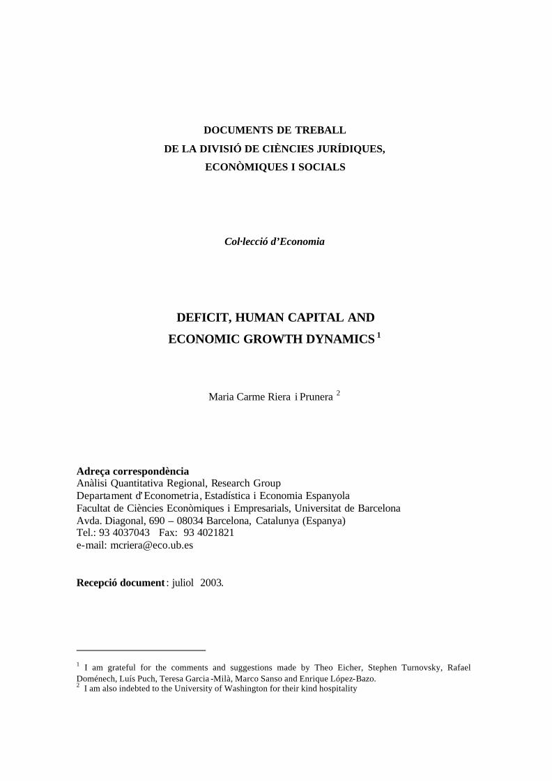
Table 1 shows that the values we employ for our fundamental parameters are in line with
those suggested by previous calibration exercises (Lucas, 1988; Jones, 1995; Ortigueira and
Santos, 1997). The final goods sector exhibits increasing returns to scale in labor and
physical capital (and knowledge). The learning sector is subject to increasing returns to
scale in human capital and government education transfers (and private expenditures).
Table 1. Benchmark parameters.
Production parameters
,48.0,268.0,36.0,2.0
1246.0,45.0,65.0,425.0,1
,335.0,6.0,45.0,46.1,1
====
=====
=====
NHKG
XEHlJ
HNKF
aaaa
a
AA
ηηηη
σσσ
Preference parameters 0.05, 0.25, 0.7, 0.30ρ θ γ ς= = = =
Depreciation and population parameters 0.05, 0.05, 0K H nδ δ= = =
Fiscal policy parameters 15.0,10.0,075.0,175.0 11 ==== τegg
Table 2 . Equilibrium values before the shock.
NY /̂ NH /̂ l~ KY /~
YC /~
R~ /X K% Relative wage
= NH ww 2.248% 2.248% 0.315 0.292 0.515 13.16% 0.225 1.815
Table 3. Equilibrium values after the shock.
NY /̂ NH /̂ l~ KY /~
YC /~
R~ /X K% Relative wage
= NH ww
2.627% 2.627% 0.326 0.259 0.569 11.68% 0.244 1.829
We group the resulting endogenous variables into three categories. The balanced per capita
growth of capital, output and knowledge; and key equilibrium ratios, including the output
capital ratio, the share of consumption in output, time devoted to education, private
expenditure in education as a percentage of physical capital; as well as the interest rate

20
value and the relative wage. The values for all these variables both before and after the
shock are presented in table 2 and table 3 respectively. According to them, per capita
output and knowledge growth at equilibrium, defined as NY /̂ and NH /̂ respectively in
the tables, is slightly above 2.6%, 0.4 percentage points more than before the deficit cut.
The equilibrium capital output ratio, KY /~ in the tables, is slightly below four, that is half
a point higher than the value before the shock. Moreover, 57% of output is devoted to
consumption, compared to the previous 51%. Around 33% of the endowment of time is
devoted to schooling, 5% more than the value they had before the shock, with 67% devoted
to production.
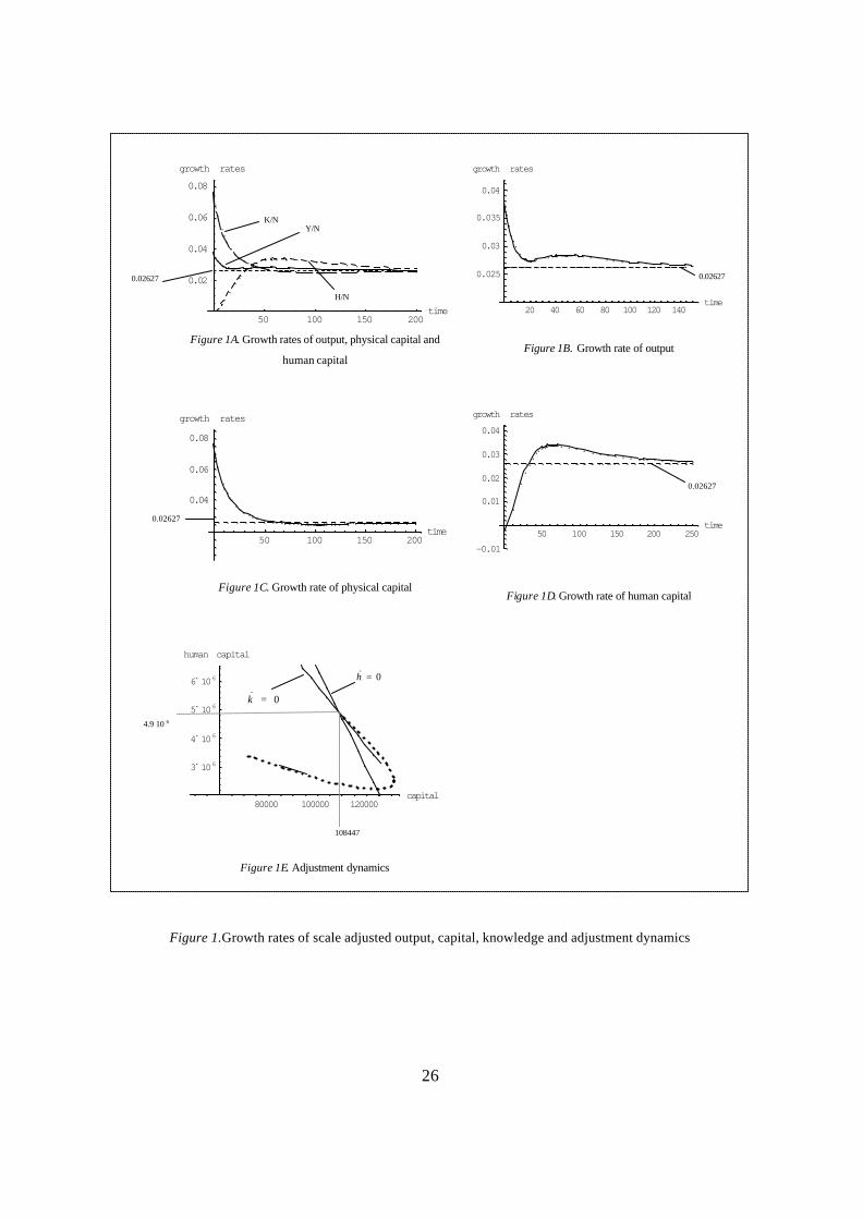
To provide clear intuition into the adjustment process, we conduct a numerical simulation8
where deficit is reduced from 12.5% to 2.5% by means of a reduction of 10 points in the
government expenditure as a percentage of GDP, g. The phase diagram (see figure 1E in
page 26) shows that the decrease in deficit and subsequent decrease in the interest rates
attracts resources first to the output production sector and away from the knowledge
production sector, with physical capital accumulating at the expense of human capital. The
figure shows how the scale-adjusted physical capital accumulates accompanied by a
reduction in the scale adjusted knowledge due to the fact that per capita rate of
accumulation of knowledge is insufficient to cover the depreciation rate. Figures 1A and 1C
show that adjusted per capita capital growth rises to above 7% during the early stages.
Within 20 periods, the growth rate of capital is reduced to half after which it falls rapidly
down towards the long-run steady state of just above 2.5%. Scale-adjusted knowledge
growth has a completely different pattern, as seen in figures 1.A and 1.D. After its initial
decline, mainly because of the rapid increase in physical capital together with the reduction
in knowledge during the early stages, it overshoots its long-run growth rate and eventually
raises the return on investing in knowledge sufficiently, relative to the return on physical
capital. With respect to the evolution of scale adjusted output growth (see figures 1A and
1B in page 26), it is worth noting that it is a combination of the two scale adjusted variables
(physical capital and knowledge). Therefore, it follows a path that lies between both of
them, adjusting faster than knowledge but slower than capital for the first 40 periods and
8 The simulations are based on the Mathematica algorithm developed by Eicher and Turnovsky (2001).

21
reversing this trend from then onwards. Scale adjusted output growth initially rises to above
3.75% but it falls sharply to around 2.75% in 20 periods, just when the decrease in physical
capital is higher. After that, it starts a mild increase during the next 30 periods, followed by
a decrease until reaching its long-run value.
The initial accumulation of physical capital attracts more time devoted to working in the
output sector, reducing the time people devote to schooling. Over time, as the growth rate
of physical capital declines and knowledge increases, the allocation of time to the
knowledge sector increases. In addition, under the assumption H Hσ η< , this rise in
knowledge further serves to drive the allocation of time from the final output sector to
schooling (knowledge producing sector). In the long-run, we end up with a higher
allocation of time to the knowledge (schooling) sector (see figure 2 in page 27). On the
other hand, the growth rate of schooling expenditures follows, in essence, the same
evolution as the allocation of time to schooling. The value of private expenditure on
education jumps down dramatically immediately after the shock and starts increasing up to
its long-run value, overshooting its previous value, hence people end up devoting more
resources to education after the shock, which changes from representing a value of 22.5%
of total physical capital up to 24.4%. The corresponding evolution is illustrated in figure 3
(page 28).
Setting life expectancy equal to its average over the sample of 90 countries that is used in
the empirical analysis of the following sect ion9, and subtracting 6 years to the original
number so as to take into account that for the first six years of life children do not go to
school, we get a value of 55.25. Using this value, our model would predict an increase of
approximately one year of schooling in the long-run, which represents a 5% increase with
respect to the original value.
Regarding the evolution of the interest rate, it starts decreasing immediately after the shock
from 13.16% down to 8.75% after 50 periods. Then, it starts increasing up to its new
equilibrium value, which is as high as 11.7%, hence around 1.5 points lower than the initial
9 See section 4.

22
one, as showed in figure 4A. It is also worth noting that although both the new raw labor
wages and skilled wages are higher after the decrease in the value of deficit. Skilled wages
have increased more relatively to unskilled wages, which translates into larger inequality
(1.5% higher measured in terms of relative wages) once the economy performs better. This
may be attributable to the fact that skilled workers have become relatively more productive,
as their stock of skills has increased, and we are considering workers being paid their
productivity. This fact is in line with the increasing inequality in salaries observed in
several economics, especially during the nineties10 and in countries whose labor market is
characterized by a higher flexibility (in countries with highly regulated labor markets, labor
market pressures have more likely translated into a higher rate of unemployment for the
less skilled).
Figure 5 shows the evolution of long-run growth as deficit changes. It is interesting noting
that once deficit has reached a very large value, further accumulation of deficit does not
imply a further decrease in growth rates, which stabilizes around -5%. In addition, we can
appreciate how a surplus situation leads to higher growth but only up to some point. Again,
this time it is worth pointing out that once surplus has reached a certain large value, it leads
to negative growth and further increases in surplus do imply further decreases in growth.
Hence these simulations give us a flavor of how damaging deficits may become, and also
how a policy that pursues larger surpluses may not be an optimal solution either, since both
deficit and surplus can be seen as two forms of disequilibrium, i.e. excessive spending and
idle resources respectively, these latter ones translated into working at a lower level than
the potential one.
3.5. Discussion
One could view long-run deficits as being determined by the economic, social or political
characteristics of a country in such a way that better fiscal and monetary policies (or with
10 Manacorda and Petrongolo, 1999; Mortensen and Pissarides, 1999.

23
better results), better management of the economy, less corruption, greater productivity,
etc., would bring an economy to a situation with lower values for deficit and, consequently,
towards a greater level of growth at equilibrium. Our work provides an enriched view of the
consequences of deficit introducing the dynamics of the economy following a change in
deficit. We believe that large values for deficit would determine a value for interest rate, R,
large enough for the agents to believe that human and physical capital accumulation was
not worth enough. In an analogous way, a value for deficit that was sufficiently low or a
certain surplus, associated with low values for R, could determine large positive values for
schooling time, l, and private schooling expenditures, x, followed by positive and optimal
growth.
Deficits are defined as the part of government expenses that are not covered with taxes. If
we think of them as a percentage of GDP it is easy to see that we are not saying that
running a certain level of deficit is largely deleterious for an economy or that an economy
should always try to avoid an increase of deficit in absolute terms. As long as the growth
rate of the economy is higher than the absolute deficit growth and if the economy has low
deficit values these latter ones should not be, in principle, a major problem, since they
would be decreasing in relative terms as a percentage of GDP. Problems arise when the
ratio of deficit with respect to GDP, d, is increasing over time and especially in the long-
run. Then, deficits may start strongly harming the economy. We do not mean that
governments should reduce their spending by all means at any time, we are only saying that
when public spending were increasing more than GDP for some periods of time, thus
generating more deficit, governments should start taking more care about public spending
because it may be that it is undertaken without following efficient requirements or that
certain expenses are under productive, hence generating macroeconomic disequilibria. In
that case governments should reduce the unproductive spending and enhance the productive
part of it, to pursue economic growth.
The model provides a long-run value for deficit, that is a steady state value reached after
one (like this case) or more shocks. The idea underlying the model is to capture a stable
value for macroeconomic disequilibria (represented by deficits) which is consistent with
reasonable economic parameters and especially with a reasonable rate of growth. If we look

24
at figure 5, we can see how deficits and surpluses are related to growth. The way we have
elaborated figure 5 is the following one. Taking (18d’) as the long-run relationship between
deficit and growth, keeping all parameters constant but deficit, we have plotted different
values for deficit with their corresponding growth values. We get the standard results for
the positive values of deficit saying that the higher the deficit, the lower the economic
growth; and that low absolute values for deficit (or even the presence of surplus) are related
to positive values for growth. In any case, the value at which deficit is related to positive
values of growth as well as the value at which surplus starts exerting a negative influence
on growth varies according to the parameters in the economy.
Given this, it is interesting to know if even small quantities of deficit resulting from
efficient government spending (i.e. infrastructures) might have a negative effect on growth.
When analyzing this, we should bear in mind that deficits are taken as the mean of several
years, thus including up and down parts of the cycle (deficitarian and surplus years). Hence,
it would be likely that we ended up with a very low value for deficit in the long-run in order
for it to be efficient. Under this situation, even current deficits initially acting as buffers in
the economic cycle may have negative effects if they become permanent throughout the
whole cycle. Consequently, a fiscal behavior like this one, which may be beneficial at
certain points of the cycle, cannot certainly be sustainable in the long-run.
At this point, we would like to cast some doubts on the goodness of surplus. The case with
the presence of surplus could be viewed as a positive situation where governments might
decide to give back the surplus into the form of transfers to agents, which could stimulate
larger values for l as well as x, (up to a certain point). Nevertheless, our present model
would not predict that any larger surplus increase translated into a better economic
situation. Indeed, a high surplus situation could also represent a sub optimal situation given
that there could be some idle resources. According to our model a budget surplus should be
related to low interest rate values and this, in turn, would make the acquisition of education
more attractive (less costly). However, increasing values of time devoted to education have
their counterpart in decreasing values of time devoted to working. As long as productivity
of working time is able to compensate for the reduced number of working hours, the
economy will go on growing. There will be a point, though, where the economy will

25
require more labor not to have idle resources (let us say capital). It will be at this point,
where surpluses may start exerting a negative influence on growth. Considering that we are
assuming the existence of complemetarity of the different productive factors, which is quite
plausible if we consider the functioning of an industry, the lack of one of these factors may
slow down the production of final output impinging a lower rate of growth to the economy.
One further implication of our model is the existence of a poverty trap: for some conditions,
the economy evolves to a low (or null) growth situation. We could think that these
economies burdening too big deficits and finishing with a low value for human capital and
growth, could adopt a different technology, which might allow them to initially increase
their production without requiring so much human capital (e.g. working in the primary
sector with a production function with physical capital as its sole inputs). Later, they could
adopt a higher technology including human capital, which would allow them to grow faster
once the economy had already taken off.
Notice that, according to our model, it is not impossible for a poor country to join the richer
ones since it only needs a favorable mix of deficit, schooling and human capital. On the
other hand, the equilibrium with growth may not be fully optimal because of the different
value given to deficit [by different agents, i.e. consumers and authorities]. So, individuals
may not be aware of the positive influence a small quantity of deficit may exert on the
economy. The performance of a Social Planner (or a fiscal authority) imposing a certain
level of deficit (optimal), larger than the one in equilibrium, depending on the
characteristics of the economy, may lead to a Balanced Growth Path where the variables H,
Y, C and K grow at constant rates different from zero and larger than the ones obtained in
this paper; and where the shadow values of both human and physical capital (m and q) slow
down at constant rates lower than the ones obtained here. At this point we could mention
some of the policies recently undertaken by the IMF, especially in low developed countries,
seeking the control of deficits, which, in most times, are tied to investments in human
capital in order to foster a higher level of economic development and growth.
26
50 100 150 200time
0.02
0.04
0.06
0.08
growth rates
Figure 1A. Growth rates of output, physical capital and
human capital
20 40 60 80 100 120 140time
0.025
0.03
0.035
0.04
growth rates
Figure 1B. Growth rate of output
50 100 150 200time
0.04
0.06
0.08
growth rates
Figure 1C. Growth rate of physical capital
50 100 150 200 250time
-0.01
0.01
0.02
0.03
0.04
growth rates
Figure 1D. Growth rate of human capital
80000 100000 120000capital
3´ 106
4´ 106
5´ 106
6´ 106
human capital
Figure 1E. Adjustment dynamics
Figure 1.Growth rates of scale adjusted output, capital, knowledge and adjustment dynamics
K/N
H/N
Y/N
0.02627 0.02627
0.02627
0.02627
0.02627
0.02627
0h =&
0k =&
108447
4.9 10 6

27
50 100 150 200 250 300 350time
0.15
0.25
0.3
0.35Schooling time
Figure 2A. Schooling time adjustment and compared
50 100 150 200time
-0.005
0.005
0.01
0.015Growth rates
Figure 2B. Growth rate of schooling time
50 100 150 200 250 300 350time
0.65
0.75
0.8
0.85
Working time
Figure 2C. Working time adjustment
Figure 2. Schooling and working dynamics.
New schooling rate = 0.326
Old schooling rate = 0.315
Old working time=0.685
New working time=0.674

28
50 100 150 200 250 300 350time
5000
10000
15000
20000
25000
30000Private expenditure
Figure 3A. Private expenditure adjustment and compared
50 100 150 200 250 300 350time
0.05
0.1
0.15
0.2
0.25
0.3Private expenditure
Figure 3B. Private schooling expenditure as a percentage of capital
Figure 3. Private expenditure on schooling and dynamics.
New expenditure =26440
Old expenditure=21167
New expenditure = 0.244
Old expenditure = 0.225

29
50 100 150 200 250 300 350time
0.08
0.09
0.110.12
0.13
0.14
0.15Interest rates
Figure 4A. Interest rate adjustment
50 100 150 200 250time
-0.03
-0.025
-0.02
-0.015
-0.01
-0.005
0.005growth rates
Figure 4B. Interest rate growth
50 100 150 200 250 300 350time
1.65
1.75
1.8
1.85relative wages
Figure 4C. Relative wages adjustment
50 100 150 200 250 300 350time
-0.0002
0.0002
0.0004
0.0006
0.0008
0.001relative wages
Figure 4D. Relative wages growth
Figure 4. Relative wages and interest rates
New interest rate=11.68%
Old interest rate=13.16%
Old relative wage=1.815
New relative wage=1.830

30
1 2 3 4 5deficit
-0.03
-0.02
-0.01
0.01
equilibrium growth
Figure 5A. Long-run growth values and deficit
-0.2 0.2 0.4 0.6deficit
0.005
0.01
0.015
0.02
0.025
equilibrium growth
Figure 5B. Long-run growth values, deficit and surplus
-15 -10 -5 5deficit
-3
-2.5
-2
-1.5
-1
-0.5
equilibrium growth
Figure 5C. Long-run growth values and surplus
Figure 5. Deficit and growth

31
Summing up, depending on long-run structural disequilibria, an economy may finish with
different equilibrium values for growth. Following that, a possible way to foster long-run
growth could come from keeping low values for deficit. These low values could be partly
determined both by a restrictive fiscal policy as well as a positive interaction between other
determinants of macroeconomic stability such as a restrictive monetary policy or a major
spending control, among other possibilities.
4. Empirical evidence
Obviously, one of the first things one comes out with when thinking about analyzing the
relationship of a macroeconomic variable or group of variables with growth is to check, in a
very preliminary way, the empirical validity of that relationship for a large number of
economies to see what the reality tells about the idea you just came out with. That is exactly
what happened when we started sketching the analysis undertaken in this paper. The first
results we got were quite satisfactory, showing a high correla tion between deficit and
growth, which allowed us to go on building the theoretical model that tried to find a
satisfactory and somehow well-founded explanation for the relationships we were
interested in analyzing. Furthermore, an extensive empirical analysis should help us to
validate our theoretical results. Actually, statistical evidence seems to support our basic
proposition that deficit may harm human capital accumulation and thus slow down growth.
The data we used have been obtained from two different sources. First, educational
attainment comes from Barro-Lee data set (1993). We have used the variable defined as the
average schooling years in the total population over age 25. Secondly, the rest of the
variables included come from the World Bank macroeconomic data sets (25/05/1999),
(http://www.worldbank.org/html/prdmg/grthweb/growth_t.htm). Although the World Bank
provides data for 212 countries, our sample of countries was fir stly reduced to
approximately one half since data on education cover roughly one hundred of them. We
also eliminated those countries that lacked all data necessary to obtain all the variables we
required. In addition, some authors have studied the problems arising in gauging human

32
capital data, such as Temple (1999b) and de la Fuente and Doménech (2000, 2001). As we
proceeded with the first empirical analysis, we came out with some extreme values for a
few countries, which motivated an outlier residual analysis that allowed us to capture some
of the outliers. By means of the Cook distance criteria, we captured the extreme values for
some countries in the sample. More especifically, for Togo, Nepal and Niger, which we
also removed out from the sample. After this, we ended up with 90 countries (see table A.3
in appendix 2).
Human capital growth is obtained as the difference between the logarithm of 1990 human
capital and the logarithm of 1970 human capital. Output growth rate has been obtained in a
similar way, taking the difference of the logs for 1990 and 1970 real per capita output. The
rest of the variables included in the analysis have been obtained as the mean for the period
1970-1990. Deficit, exports, imports and government spending have been taken as a
percentage of the GDP in each country. We have used the series budget surplus including
grants from the World Bank for the deficit.
Goetz and Hu (1996) estimate human capital growth as a function of what they came to call
environmental variables, which they chose based on previous studies. Most of those studies
were based on individual polls. In addition, Cameron and Heckman (1993) assert that the
decision to undertake university studies depend on some aspects such as the father’s
occupation or the house property; Cohn and Hughes (1994) add the unemployment tax, the
mean salary and the size of the city, the latter one in order to capture the likely
agglomeration effects. Goetz and Hu say that taking countries as an aggregate, there are
variables such as employment, which are difficult to obtain, therefore the regressors they
end up using are urbanization, in order to capture the effects coming from the size of the
city, unemployment, the percentage of owned houses, the size of the family, the level of
local taxes per capita, the education expenditures, as well as the percentage of professionals
in the labour market.
In order to test for the influence as well as the robustness of deficit as an important
determinant for human capital growth and economic growth, following the literature (Goetz
and Hu, 1996; Easterly and Rebelo, 1993; Fisher, 1993), we have taken into account

33
different groups of regressors related to different aspects of the economy that may influence
this relationship. More specifically, we have introduced production (initial output and
output growth) and trade (exports plus imports), Rivera-Batiz and Romer, 1991. The
inclusion of trade relies on the assumption that a larger openness degree may have
stimulative effects on the acquisition of human capital. We decided to introduce political
and social instability variables (coups, assassinations, revolts ) as a factor which may
disincentive training, given that the economy may allocate resources away from education.
Other variables introduce were location variables (urbanization percentage and latitude, as
well as a dummy variable, R4 , which tries to capture the likely regional effects coming
from eastern Asia); government spending (education, health, defense), not only direct
government spending on education but also on defense, as a possible deterrent of other
types of expenditure, which may report higher social benefits, and health , given its direct
relationship with human capital accumulation, especially in low developed countries.
Besides, there are some further aspects relating health with growth, such as the
demographic structure or various sanitary issues; monetary aspects (M2, real interest rates,
exchange rates, inflation and black market premium (BMP)), all of them trying to capture
the necessary stability required by the agents to form favorable future expectations that
bring them to choose a higher value for schooling at present; demographic aspects (life
expectancy) in order to capture the fact that a higher availability of time might increase the
time agents devote to education; and government tax collection, following Nerlove et al.
(1993). Given that we have introduced several variables, we should note that this might be
quite a rigorous exercise; since one has to bear in mind that deficit may be inf luencing
some of these variables we have used as regressors.
Table A.1 summarizes the results on human capital accumulation. Equation 1 shows the
positive relationship between human capital growth and surplus (negative relation with
deficit, which is take n with a negative sign), being significant at 10% level. However, this
equation may be subject to a wrong specification given that we have omitted the value for
initial human capital. Hence, we would not be taking into account the possibility of human
capital convergence across countries. Equation 2, with initial human capital, shows its
importance as an explanatory variable in the acquisition of education. Most of the
regressions onwards show the likely presence of catching-up in terms of education as its

34
coefficient takes a highly significant negative value. This value shows the existence of
convergence in human capital terms among countries, which could be understood as the
presence of decreasing returns to scale of human capital stock in the knowledge equation,
thus validating the assumption made in the theoretical part of the paper. Besides, equation 2
allows us to test for the influence of deficit in human capital growth, being significant at
1.1% level. Hence, the first two equations might be confirming the discouraging effect that
deficit seems to generate when accumulating human capital. The results we got for the
various regressions seem to confirm the robustness of deficit to the inclusion of different
economic aspects with respect to its significance level, except for the variables related to
output (initial output and output growth), location (urbanization), and life expectancy,
despite the fact that, as seen in the various specifications, the size of the coefficient for the
deficit varies depending on the specification of the regression. On the other hand, the sign
of the deficit is the expected one in all the cases analyzed with the exception of output
growth and initial output. With respect to the hypothesis of trade, data does not seem to
confirm it, since the coefficient on trade is not significant at all. Besides, it is quite
surprising the lack of significance of the coefficient of government spending on education
as well as health, given the likely a priori influence of both on schooling. Finally, we have
introduced the last regression including all the regressors as a matter of completeness. We
should highlight the solely significance of the following variables: initial human capital
(1%), deficit (1%), trade (5%), assassinations (1%), riots (5%), latitude (5%), monetary
aggregate (1%), life expectancy (1%) and taxes (1%). However, it is worth mentioning that
the introduction of the whole range of variables may be hindering some of the
interinfluences, and thus a likely high degree of multicollinearity with the subsequent
problems related to it, which somehow reduces the confidence level of this last regression.
To sum up, we could say that deficits have a strong negative relationship with human
capital growth in such a way that a 1 percentage point increase in deficit would translate
into a reduction of 0.3-0.6 percentage points in human capital growth. Besides, it is worth
noting that we have undertaken an empirical linear analysis. Actually we pretend it to be
the starting point of a likely more extended analysis, which might be able to capture, in the
near future, some of the non-linearities previously presented in the theoretical part.
35
In order to validate our theoretical model as well as to test for the influence of deficits on
economic growth and compare our results to the ones previously obtained (Fischer,
1993a,b; Easterly and Rebelo, 1993), we have undertaken a cross-section analysis for the
GDP growth. The dependent variable used has been output growth, whereas the rest of the
variables are the ones used in the previous analyses. In the extensions of the neoclassical
model (Mankiw, Romer and Weil, 1992) as well as in endogenous growth models (Lucas,
1988), economic growth rate is a function of two state variables, named physical capital
and human capital. In later models, Becker, Murphy and Tamura (1990) and Azariadis and
Drazen (1990), the initial value for human capital is taken as an important determinant for
future growth. Easterly and Rebelo (1993) include monetary aspects (M2) as well as trade
and try to keep constant the effects of some policies which other authors such as Levine and
Renelt (1992) or King and Levine (1993) have shown to be robustly correlated with
economic growth.
Given that the choice of regressors used in the literature in order to analyze growth varies
quite a lot with respect to the framework of study as well as to the limits coming from the
availability of the data, we have undertaken the inclusion of the variables according to the
various empirical studies in the literature. Thus, deficit has been included in order to test for
the economic growth distortions that deficit can induce basically when taken as an indicator
for macroeconomic disequilibria, (Levine and Renelt, 1992; Levine and Zervos, 1994;
Easterly and Rebelo, 1993; Fischer, 1993a,b; Esterly and Levine, 1997). Based on previous
analyses, we have introduced human capital growth as well as initial human capital, since
the first one has been identified as one of the aspects that exerts a larger influence on
economic growth (e. g. Denison, 1984), whereas the value for initial human capital allows
us to test for the influence of starting points. This last one would be related to the so called
level effects, which can be seen as a requirement to adopt ongoing innovations; trade
(Cornwall, 1976; Harrison, 1996; Frankel and Romer, 1996; Miller and Russek, 1997);
social instability, (Alesina et al., 1996; Caselli et al., 1996; Sachs and Warner, 1995);
latitude (Sala-i-Martín, 1997); government expenditures , (Levine and Renelt, 1992;
Knowles and Owen, 1995; Barro, 1997); monetary aspects, (Kormendi and Meguire, 1985;
Dollar, 1992; Fischer, 1993b; Englander and Gurney, 1994; Harrison, 1996; de Gregorio,
1996; Andrés and Hernando, 1997); life expectancy and population growth , (Kormendi and

36
Meguire, 1985; Dowrick and Nguyen, 1989; Mankiw, Romer and Weil, 1992; Barro and
Lee, 1994; Lee, 1995); and taxes (Miller and Russek, 1997; Kneller et al., 1998).
Results on annual average growth rates of per capita real GDP are summarized in table A.2.
We can observe, as shown by equations 14 and 15 , the presence of a large influence of
deficit on growth. This result would confirm the theoretical long-run relationship, where
long-run growth was established to depend negatively on the deficit value. From equation
15 onwards we have introduced a convergence mechanism including initial output in order
to capture the possible convergence process. We should note that equation 15 tells us that
the introduction of initial output solely, without initial human capital, does not work as a
convergence mechanism, as shown by Baumol (1986), among other authors. Certainly,
from there onwards, with the initial values for both variables, output and human capital, we
do obtain convergence.
In order to test for the robustness of the deficit, we have added some other variables
referred to different aspects of the economy. The results we obtained confirm the
robustness of deficit with respect to its significance level. Our results allow us to capture
the fact that the size of the influence of the deficit on growth does not change in the
different specifications, with the exception of monetary variables that seem to relax a bit
the significance of deficit and specially inflation. On the other hand, the sign of the
coefficient is always the right one. The values we get for the coefficient on deficit in the
various regressions undertaken are between 0.10 and 0.17, in line with the ones obtained in
the previous empirical studies, (Easterly and Levine, 1997; Fischer, 1993b), which are
between 0.1 and 0.25. This would mean that a one -percentage point increase in the value of
deficit translates into around 0.15 percentage points decrease in growth. Finally, we have
introduced all the regressors. In this case, the coefficient of deficit is significant only at
17%, and it even has a much lower magnitude. However, the exclusion of monetary
variables, as showed in equation 26 , leads to a highly significant coefficient for the deficit.
That could be somehow showing the likely presence of correlation between fiscal and
monetary policies, which could be distorting the results. On the other hand, it should be
mentioned that the only significant variables appear to be initial income (1%), deficit (5%),

37
latitude (5%), defense expenditure (5%), life expectancy (1%) and population growth
(10%).
In sum, our results confirm the hypothesis presented in the theoretical model when we
considered a situation where economic disequilibria, as represented by deficits, could exert
a negative influence on economic growth in the sense that smaller deficits are associated
with faster growth by means of higher human and physical capital accumulation.
5. Conclusion
When looking at the evolution of the economy, one observes how several countries have
experienced large periods of sustained growth (Kaldor, 1961), although one can also see the
presence of a large dispersion in income across countries or geographical locations (Galor
and Zeira, 1993). Several studies have tried to shed light on this fact by using models
dealing with capital varieties, improvements in the quality of products or diffusion of
technology, among others. Differences in monetary and fiscal policies that have been
applied by different economies may also partly explain the different economic performance
of several countries during the last decades. Nevertheless, as posed by Romer (1989), in
order to explain increases in income as well as in growth rates, it may be enough if we
concentrate on variables such as schooling and human capital accumulation. In this paper,
we have been mainly concerned about the behavior of the government and its fiscal policy,
more specifically, about the presence of macroeconomic disequilibria in a country that we
have defined in terms of budget deficits or fiscal imbalances that are capturing government
mismanagement of an economy, and sub-optimal allocation of resources. Given the
difficulty in defining and gauging [in]stability in a macroeconomic framework, some
authors like Fischer (1993b) have specified some stability indicators, mainly centered on
deficitarian aspects of an economy. In fact, budget deficits seem to be a macroeconomic
indicator that appears in most of the analysis performed to capture the influence of
macroeconomic stability on economic growth and it turns out to be one of the most
influencing economic variables in this respect.

38
If we graph the evolution of long-run deficits for different countries (taking deficit as a
percentage of GDP) we could appreciate how most of them decrease over time and tend to
stabilize at different positive values within different groups of countries. That is to say that
there seems to be different convergence values for deficit, depending on the parameters of
the economy. According to this, and taking into account that different values of deficit may
be related to different interest rate values, in this paper, we have introduced the possibility
that the choice of schooling private investment depended on the presence of
macroeconomic disequilibria. A simple model of growth that links deficit and human
capital with economic growth has been posed. It considers deficit as a harmful aspect for an
economy mainly when characterized by persistency and largeness. We have shown that
long-run growth differences across countries may depend on their different disequilibria,
thus determining the existence of poverty traps for economies with high budget imbalances,
and positive rates of growth for those with low (or null) imbalances. This paper goes further
away introducing the dynamics of the economy following a change in deficit. It shows the
evolution of human and physical capital as well as the change in schooling time, interest
rates or relative wages after a fiscal shock. In this sense, we could conclude that a value for
deficit that were sufficiently low would be associated with low interest rate values, which
would determine high values for private schooling expenditures (and schooling time).
Large deficits that have been reached after periods of excessive spending by the
government, which may not disappear and become permanent, due to the nature of
spending, are the most likely to exert deleterious effects on growth. Investing in wrong
conceived projects (e.g. defense programs, temporary consumption) may not induce
economic growth either. Therefore, under these circumstances, large permanent deficits
could be weakening the economy. According to our model and taking into account the set
of parameter values we used, a decrease of 10 basis points in deficit from 12.5 to 2.5 would
finish increasing by around 5% the initial time people devoted to schooling. Besides,
underlying our results, in high deficit economies there could be a reduction not only in
resources and time itself but also in the efficiency of time devoted to education either
because of a lack of resources or because it is simply approaching the mismanagement of
the economy. Furthermore, low values for deficit that could be acknowledging a superior
management of an economy, or a better distribution of resources, may translate into a better
39
working of the education system, meaning greater efficiency of human capital
accumulation and larger per capita income growth.
On the other hand, the broad range of evidence reviewed and presented here seems to
support such effects. Regarding the empirical evidence, using data for a large sample of
countries during the period 1970-1990, the results we obtained seem to support the idea that
deficits may be negatively related to human and physical capital accumulation, mainly due
to the burden impinged on both physical and human capital. Our results would be in line
with the ones previously obtained in the literature, relating deficitarian situations negatively
with growth. More specifically, we found that a 1 percentage point increase in deficit would
translate into a human capital growth reduction of about 0.5 percentage points. On the other
hand, regressing deficit on output growth gives that a one percentage point increase in
deficit is related to approximately 0.15 percentage points decrease in growth, in line with
the results obtained in the literature (Easterly and Levine, 1997; Fischer, 1993b).
Taking all this into account, one of the possible solutions to reduce income and growth
inequality could be to provide external economic finance for the countries facing high
deficits and low growth values under the form of subsidies to interest rates in order to
finance a percentage of them when they happen to be far above a certain level. In any case,
aid renewal should be tied down to periodic revisions, seeking the fulfillment of certain
goals, mainly to devote the subsidies to finance schooling as well as to a better
macroeconomic performance of the economy.
Furthermore, despite the generally attributed goodness of surplus, our present model would
not predict that larger surpluses translated into a better economic situation. Indeed, a high
surplus situation could also represent a sub optimal situation given that there could be some
idle resources in the economy. This could mean that the economy was not working at its
full potential level, thus wasting resources.
Passing now to other matters, one could believe that it is not only time devoted to education
what helps improving human capital of agents who get education, but also the quality of the
education acquired. We suspect that quality or effectiveness of training might be closely

40
related to macroeconomic stability. Also, the distribution of government budget and the
good or bad management of the economy could be an interesting aspect to go deep into in
future research so as to find possible answers as well as solutions for the bad performance
of some economies, once macroeconomic disequilibria are defined in more detail.
References
Alesina, A., A.S. Ozler, N. Roubini and P. Swagel (1996): “Political instability and economic growth”, Journal of Economic Growth, vol. 1, pp. 189-211. Andrés, J. and I. Hernando (1997): “Does inflation harm economic growth? Evidence for the OECD”, NBER Working Paper, nº 6062. Azariadis, C. and A. Drazen, (1990):“Threshold externalities in economic development”, Quarterly Journal of Economics, vol. 105, nº 2, pp. 501-526. Ballabriga, F.C. and M. Sebastian (1993): “Deficit público y tipos de interés en la economía española: existe evidencia de causalidad?”, Revista Española de Economía, vol. 10, nº 2, pp. 283-306. Barro, R.J. (1997): “Determinants of economic growth: a cross -country empirical study”, Harvard Institute for International Development, Discussion Paper, Discussion Paper, nº 579. Barro, R. (1990): “Government spending in a simple model of economic growth”, Journal of Political Economy, vol. 98, pp. S103-S125. Barro, R., (1989), “The Ricardian approach to budget deficits ”, Journal of Economic Perspectives vol. 3, nº 2, pp. 33-54. Barro, R., 1974, “Are government bonds net wealth?”, Journal of Political Economy, vol. 82, nº 6, pp. 1095-1117. Barro, R. and J. Lee (1994), “Sources of economic growth”, Carnegie-Rochester Conference Series on Public Policy, vol. 40, nº 0, pp. 1-46. Barro, R. and J. Lee, (1993), “International comparisons of educational attainment”, Journal of Monetary Economics, vol. 32, nº 3, pp. 363-394. Baumol, W.J. (1986): “Productivity growth, convergence and welfare: what the long run data show”, American Economic Review, vol. 76, nº 5, pp. 1072-1085. Becker, G.S., K.M. Murphy and R. Tamura (1990): “Human capital, fertility and economic growth”, Journal of Political Economy, vol. 98, nº 5, pp. S12-S37.

41
Benhabib, J. and M. Spiegel, 1994, “The role of human capital in economic development. Evidence from aggregated cross-country data, Journal of Monetary Economics , vol. 34, nº 2, pp. 143-173. Blanchard, O.J. (1985): “Debt, Deficits, and Finite Horizons”, Journal of Political Economy, vol. 93, n. 2, pp. 223-247. Blanchard, O.J. and S. Fischer (1989): Lectures on Macroeconomics, MIT Press, Cambridge, Massachusetts. Boskin, M., (1988):“ Concepts and measures of federal deficits and debt and their impact on economic activity”, in The economics of public debt, MacMillan Press, Hampshire. Bowles, D., H. Ulbrich and M. Wallace (1989): “Default risk, interest differentials and fiscal policy: a new look at crowding-out”, Eastern Economic Journal, vol. 15, n. 3, pp. 203-212. Card, C. and A.B. Krueger (1992): “Does School Quality Matter? Returns to Education and the Characteristics of Public Schools in the United States”, Journal-of-Political-Economy, vol. 100, n. 1, pp. 1-40. Cameron, S. and J. Heckman (1993): “Determinants of young male schooling and training choices”, National Bureau of Economic Research Working Paper, n. 4327. Carmichael, J., (1982): “On Barro’s theorem of debt neutrality: the irrelevance of net wealth”, American Economic Review, vol. 72, nº 1, pp. 202-213. Caselli, F., G. Esquivel and F. Lefort (1996): “Reopening the convergence debate: a new look at cross-country growth empirics”, Journal of Economic Growth, vol. 1, nº 3, pp. 363-389. Cebula, R. and C. Hung, (1992): “Government budget deficits and interest rates: an empirical analysis for the United States and Canada”, Rivista Internazionale di Scienze Economiche e Commerciali, vol. 39, nº. 10-11, pp. 917-928. Cebula, R.J. (1991): “Federal budget deficits and the term structure of real interest rates”, Southern Economic Journal, vol. 57, pp.1170-1173. Cebula, R.J. (1988): “Federal government budget deficits and interest rates: a brief note”, Southern Economic Journal, vol. July, pp.206-210. Cohn, E. And W.W. Hughes (1994): “A benefit-cost analysis on investment in college education in the United States: 1969-1985”, Economics of Education Review, vol. 13, pp. 109-123. Cornwall, J. (1976): “Diffusion, convergence and Kaldor’s law”, Economic Journal, vol. 86, nº 342, pp. 307-314.

42
Darrat, A.F. (1989): “Federal budget deficits and long-term interest rates: further evidence from annual data”, Southern Economic Journal, vol. October, pp.363-374. Davies, J. and J. Whalley, (1989): “Taxes and human capital formation: how important is human capital?”, NBER working paper nº 2899. De Gregorio, J. (1996): “Inflation, growth and central banks: theory and evidence”, Mimeo. De la Fuente, A. and R. Doménech (2000): “Human capital in growth regressions: how much difference does data quality make?, Institut d’Anàlisi Econòmica (CSIC) and Universitat de València, Mimeo. De la Fuente, A. and R. Doménech (2001): “Schooling data, technological diffusion and the Neoclassical model”, American Economic Review, vol. 91, n. 2, pp. 323-327. Denison, E.E. (1984): “Accounting for slower economic growth: an update in J.W. Kendrick, ed., International comparisons of productivity and causes of the slowdown , Ballinger, Cambridge. Devereux, M.B. and D.R. Love (1995): “The dynamic effects of government spending policies in a two-sector endogenous growth model”, Journal of Money, Credit and Banking, vol. 27, n. 1, pp. 232-257. Diamond, P., (1965): “National debt and Neoclassical economic growth”, American Economic Review, vol. 55, nº 5, pp.1126-1150. Dollar, D. (1991): “Outward-oriented developing economies really do grow more rapidly: evidence from 95 LDCs, 1976-85”, Economic Development and Cultural Change. Doménech, R., D. Taguas and J. Varela (2001): “The effects of budget deficit on national saving in the OECD”, Economics Letters, vol. 91, n. 2, pp. 323-327. Dowrick, S. and D.T. Nguyen (1989): “OECD comparative economic growth 1950-1985: catch-up and convergence”, American Economic Review, vol. 79, nº 5, pp. 1010-1030. Drazen, A., (1978): “Government debt, human capital and bequests in a life-cycle model”, Journal of Political Economy, vol. 86, nº 3, pp. 505-516. Easterly, W. and R. Levine, (1997): “Africa's growth tragedy”, Quarterly Journal of Economics , vol. 74, pp. 1203-1250. Easterly, W. and S. Rebelo (1993): “Fiscal policy and economic growth”, Journal of Monetary Economics, vol. 32, pp. 417-449. Eicher, T. and S.J. Turnovsky (2001): “Transition dynamics in non-scale models”, Journal of Economic Dynamics and Control, vol. 25, pp. 85-113.

43
Eisner, R and P. Pieper (1988): “Deficits, monetary policy and real economic activity”, in The economics of public debt, MacMillan Press, Hampshire, 1988. Eisner, R., (1989): “Budget deficits: rhetoric and reality”, Journal of Economic Perspectives, vol. 3, nº 2, pp. 73-93. Englander S., and A. Gurney (1994): “Medium-term determinant of OECD productivity”, OECD Economic Studies, Spring, nº 22, pp. 17-45. Esteve, V. y C.R. Tamarit, (1996): “Déficit públicos, expectativas inflacionarias y tipos de interés nominales en la economía española”, Moneda y Crédito , nº 203, pp. 11-41. Evans, P. (1985): “Do large deficits produce high interest rates?”, American Economic Review, vol. March, pp.68-87. Evans, P. (1987): “Do budget deficits raise nominal interest rates? Evidence from six countries”, Journal of Monetary Economics, vol. 00, pp.281-300. Fischer, S. (1993a): “Growth, macroeconomics and development”, NBER Macro-economics Annual, pp. 329-364. Fischer, S. (1993b): “The role of macroeconomic factors in growth”, Journal of Monetary Economics, vol. 32, n. 3, pp. 485-512. Frankel, J.A. and D. Romer, (1996): “Trade and Growth: An Empirical Investigation”, National Bureau of Economic Research Working Paper. Glomm, G. and B. Ravikumar (1995): “Public versus Private Investment in Human Capital Endogenous Growth and Income Inequality”, Journal of Political Economy, vol. 100, n. 4, pp. 813-834. Gale, D., (1973): “Pure exchange equilibrium of dynamic economic models”, Journal of Economic Theory, pp. 12-36. Galor, O. and J.Zeira, (1993): “Income Distribution and Macroeconomics”, Review of Economic Studies, 60(1), pages 35-52. Goetz, S and D. Hu, (1996): “Economic growth and human capital accumulation: simultaneity and expanded convergence tests”, Economics Letters, vol. 51, pp. 355-362. Goisis, G., (1989): “Budget deficit and interest rates”, Rivista Internazionale di Scienze Economiche e Commerciali, vol. 36, nº. 10-11, pp. 887-903. Hansson, I. and C. Stuart, 1987, “The welfare costs of deficit finance”, Economic Inquiry, vol. 25, nº 3, pp. 479-496. Harrison, A. (1996): “Openness and growth: a time-series, cross-country analysis for developing countries”, Journal of Development Economics, vol. 48, pp. 419-447.

44
Harrison, A. (1996): “Openness and growth: a time-series, cross-country analysis for developing countries”, Journal of Development Economics, vol. 48, pp. 419-447. Ihori, T., (1988): “Debt burden and intergeneration equity”, in The economics of public debt, MacMillan Press, Hampshire. Jones, C. I. (1995): “Time-series tests of endogenous growth models”, Quarterly Journal of Economics , vol. 110, pp. 495-525. Kaldor, N. (1961): “Capital accumulation and economic growth”, in F. Lutz (ed.), The theory of Capital, London, Macmillan. King, R.G. and R. Levine (1993): “Finance and growth: Schumpeter might be right”, Quarterly Journal of Economics, vol. 108, nº 3, pp. 717-737. Kneller, R., M. Bleaney and N. Gemmell (1998): “Growth, public policy and the government budget constraint: evidence from OECD countries”, University of Nottingham, School of Economics, Discussion Paper , nº 98/4. Knowles, S. and P.D. Owen (1995): “Health capital and cross-country variation in income per capita in the Mankiw-Romer-Weil model”, Economics Letters, vol. 48, nº 1, pp. 99-106. Kormendi, R.C. (1983): “Government debt, government spending and private sector behavior”, American Economic Review, vol. 73, pp.994-1010. Kormendi, R.C. and P.G. Meguire (1985): “Macroeconomic determinants of growth”, Journal of Monetary Economics, vol. 16, pp. 141-193. Lee, J.W. (1995): “Capital goods imports and long-run growth”, Journal of Development Economics, vol. 48, pp. 91-110. Levine, R. and D. Renelt (1992): “A sensitivity analysis of cross-country growth regressors”, American Economic Review, vol. 82, nº 4, pp. 942-963. Levine, R. and S. Zervos, 1994. “What We Know about Policy and Growth from Cross-Country Analysis”, in Economic growth and the structure of long-term development: Proceedings of the IEA conference held in Varenna, Italy, IEA Conference Volume, no. 112, New York, St. Martin's Press, pp. 22-44. Lucas, R., 1988, “On the mechanics of economic development”, "Journal of Monetary Economics" , vol. 22, nº. 1, pp. 3-42. Manacorda, M. and B. Petrongolo (1999): "Skill mismatch and unemployment in OECD countries", Economics, vol. 66, pp. 181-207. Mankiw, N.G. (1992): Macroeconomics , New York, Worth.

45
Mankiw, N.G., D. Romer and D.N. Weil (1992): “A contribution to the empirics of economic growth”, Quarterly Journal of Economics, vol. 107, nº 2, pp. 407-437. Miller, S.M. and F.S. Russek (1997): “Fiscal struc tures and economic growth at the state and local level”, Public Finance Review, vol. 25, nº 2, pp. 234-253. Mortensen, D., and C. Pissarides (1999): "Unemployment responses to skill-biased technology shocks: the role of labour market policy", The Economic Journal, vol. 109, pp. 242-265. Nerlove, M.A.,A. Razin, E. Sadka and R.K. von Weizsäcker (1993): “Comprehensive income taxation, investments in human and physical capital, and production”, Journal of Public Economics, vol. 50, pp. 397-406. Ortigueira, S. and M. S. Santos (1997): “On the Speed of Convergence in Endogenous Growth Models”, American Economic Review, vol. 87, nº 3, pp. 383-399. Pontryagin, L.S. (1962): The mathematical theory of optimal processes, Interscience, New York, 1962. Rivera-Batiz, L. and P. Romer (1991): “International trade with endogenous technical change”, ”, European Economic Review, vol. 35, pp. 971-1001. Romer, P. (1989): “Human capital and growth: theory and evidence”, NBER WP nº 3173. Romer, P. (1986): “Increasing retur ns and long-run growth”, Journal of Political Economy , vol. 94 (5), pp. 1002-1037. Sachs, F. and A. Warner (1995): “Economic reform and the process of global integration”, Brookings Papers on Economic Activity, vol. 1, pp. 1-118. Sala-i-Martin (1997): “I just run two million regressions”, AEA Papers and Proceedings, vol. 87, nº 2, pp. 178-183. Sánchez-Losada, F. (1998): “On the relationship between education and growth”, Universitat Autònoma de Barcelona and Institut d’Anàlisi Econòmica (CSIC), Working Paper, n. 408.98. Sargent, T.J. and N. Wallace (1994): “Some unpleasant monetarist arithmetic”, in The rational expectations revolution: Readings from the front line, Miller, P.J. (ed.), Cambridge, Mass. and London, MIT Press, pp. 103-129. Tanzi, V. And M. Blejer, (1988): “Public debt and fiscal policy in developing countries”, in The economics of public debt, MacMillan Press, Hampshire.

46
Tanzi, V. and M.S. Lutz (1985): “Fiscal deficits and interest rates in the United States: an empirical analysis, 1960-1984”, International Monetary Fund, Staff Papers, vol. 32, nº. 4, pp. 551-576. Temple, J. (1999a): “A positive effect of human capital on growth”, Economics Letters, vol. 65, n. 1, pp. 131-134. Temple, J. (1999b): “The new growth evidence”, Journal of Economic Literature, vol. XXXVII, pp. 112-156. Trostel, P., (1995): “The effect of deficit finance on human capital”, National Tax Journal, vol. 48, nº 4, pp. 531-545. Turnovsky, S.J. (2000a): “Fiscal policy, elastic labor supply and endogenous growth”, Journal of Monetary Economics, vol. 45, n. 1, pp. 185-210. Turnovsky, S.J. (2000b): “The transitional dynamics of fiscal policy: long-run capital accumulation, and growth”, University of Washington, Mimeo. Turnovsky, S.J. (1997): “Fiscal policy in a growing economy with public capital”, Macroeconomic Dynamics, vol. 1, n. 3, pp. 615-639. Turnovsky, S.J. (1989): “The term structure of interest rates and the effects of macroeconomic policy”, Journal of Money, Credit and Banking, vol. 21, n. 3, pp. 321-347. Van der Ploeg, F. and G. Alogoskoufis, (1994): “ Money and endogenous growth”, Journal of Money, Credit and Banking, vol. 26, nº 4, pp. 771-791. White, H., (1980), “A heteroscedasticity- consistent covariance matrix estimator and a direct test for heteroscedasticity”, Econometrica, vol. 48, nº 4, pp.817-838. World Bank, (1999), Macroeconomic Data set, http://www.worldbank.org/html/prdmg/grthweb/growth_t.htm (20/05/2000).

47
Appendix 1. Empirical results.
Table A.1. Human capital growth equation. Dependent variable, GH: ln(H90)-ln(H70)*, **.
Eq. 1 Eq.2 Eq.3 Eq.4 Eq.5 Eq.6 Eq.7 Eq.8 Eq.9 Eq.10 Eq.11 Eq.12 Eq.13 Constant 0.5 a 0.8 a -0.1 0.79 a 0.87 a 0.73 a 0.81 a 0.8 a 1.12 a 0.77 a -3.04 a 0.81 a -3.37 a Constant (0) (0) (0.65) (0) (0) (0) (0) (0) (0.0022) (0) (0) (0) (0.0093) H70 -0.32 a -0.44 a -0.32 a -0.34 a -0.38 a -0.34 a -0.35 a -0.32 a -0.33 a -0.49 a -0.35 a -0.54 a H70 (0) (0) (0) (0) (0) (0) (0) (0) (0) (0) (0) (0) Surplus 0.7 c 0.58b -0.11 0.56 b 0.6 a 0.32 0.53 b 0.78 a 0.51 b 0.64 a 0.29 0.51 b 0.94 a Surplus (Deficit) (0.08) (0.011) (0.79) (0.011) (0.0069) (0.17) (0.014) (0.0009) (0.045) (0.0028) (0.2) (0.026) (0.003) (Deficit) Y70 0.12 a GY (0.0001) GY 2.5 b Y70 (0.03) Trade 0.0005 0.002 b Trade (0.2) (0.01) Coups -0.56 0.08 Coups (0.17) (0.86) Assas -0.0098 -0.073 a Assas (0.68) (0.009) Revols -0.033 0.14 Revols (0.67) (0.58) Riots -0.006 0.038 b Riots (0.65) (0.02) Urban 0.0023 b 0.0023 Urban (0.02) (0.11) Latitude 0.0016 a 0.002 a 0.0017 Latitude (0.0039) (0.0015) (0.01) b R4 -0.031 -0.08 -0.14 R4 (0.74) (0.33) (0.31) Education 0.0029 -0.02 Education (0.83) (0.12) Defense 0.01 c 0.009 Defense (0.08) (0.18) Health 0.0084 0.014 Health (0.47) (0.31) M2 0.0005 0.001 c -0.003 a M2 (0.56) (0.08) (0.005) Interest 0.0014 -0.0003 2.25·10-6 Interest (0.5) (0.67) (0.99) XR -0.067 -0.15 XR (0.33) (0.05) BMP -0.00005 6.27·10-5 BMP (0.78) (0.81) Inflation 0.0002 c -0.0002 Inflation (0.10) (0.16) Life 0.97 a 1.26 a Life (0) (0.0002) Taxes -0.0011 -0.008 a Taxes (0.63) (0.0005) N 90 90 86 88 90 89 89 70 72 82 90 74 55 N R2 0.01 0.75 0.79 0.74 0.76 0.78 0.77 0.77 0.72 0.75 0.85 0.76 0.87 R2 F 0.98 131 80 83 45 60 71 44 24 58 126 75 12 F
Note: OLS results are robust to White (1980) heteroscedasticity correction method. Note: a 1%confidence level; b 5% confidence level; c 10% confidence level. * Deficit values have been taken with a negative sign, whereas surplus values have been taken with a positive sign. ** P -values of the regression coefficients are in parenthesis.

48
Table A.2 .Output growth equation. Dependent variable, GY : ln(Y90)-ln(Y70)*, **.
Eq. 14 Eq.15 Eq.16 Eq.17 Eq.18 Eq.19 Eq.20 Eq.21 Eq.22 Eq.23 Eq.24 Eq.25 Eq.26 Constant 0.018ª 0.0006 0.072ª 0.064ª 0.09ª 0.126ª 0.095ª 0.12 b 0.11ª -0.306ª 0.08ª -0.070 -0.23 c Constant (0) (0.96) (0.0012) (0.0043) (0.0003) (0) (0) (0.012) (0) (0.0006) (0.0036) (0.63) (0.01)
Y70 0.0023 -0.012ª -0.008ª -0.010ª -0.0171ª -0.012ª -0.015 a -0.015ª -0.019ª -0.01 c -0.025 a -0.024ª Y70 (0.16) (0) (0.0052) (0.0014) (0.0001) (0.0006) (0) (0) (0) (0.063) (0.0001) (0) Surplus 0.1b 0.097 b 0.12 b 0.13 b 0.15 b 0.14 b 0.16 c 0.07 0.11 b 0.13 b 0.14 b 0.019 0.17 b Surplus (Deficit) (0.02) (0.036) (0.046) (0.0388) (0.02) (0.0119) (0.055) (0.18) (0.025) (0.019) (0.045) (0.78) (0.04) (Deficit) H70 0.029ª 0.013ª 0.015ª 0.016ª 0.016ª 0.015ª 0.015ª 0.0006 0.014ª 0.016 0.0033 H70 (0.0001) (0) (0) (0) (0.0001) (0) (0) (0.84) (0.0007) (0.17) (0.75) GH 0.032 a 0.013 -0.0043 G H (0.01) (0.43) (0.8) Trade 0.0001ª -7.6·10 -5 -7·10 –5c Trade (0.0001) (0.60) (0.15) Coups -0.003 -0.091 -0.21 Coups (0.25) (0.15) (0.65) Assas -0.002 -0.002 -0.001 Assas (0.42) (0.33) (0.63) Revols -0.015 c 0.027 -0.015 Revols (0.08) (0.32) (0.37) Riots 0.0011 0.0002 0.002 c Riots (0.41) (0.87) (0.07) Urban 0.0001 -7.5·10 -5 -6.48·10 - Urban (0.33) (0.68) (0.71) Latitude 0.0002ª 0.0002 c 0.0002 c Latitude (0.0003) (0.06) (0.04) R4 -0.0007 -0.02 c -0.014 c R4 (0.87) (0.07) (0.07)
Education 0.0004 0.0003 -1.3 10-5 Education (0.68) (0.86) (0.99) Defense 0.001 c -0.0003 0.0001 c Defense (0.07) (0.81) (0.013) Health 0.001 -0.001 -0.0007 Health (0.28) (0.49) (0.59) M2 0.0003ª 0.0003ª 0.0002 M2 (0.0002) (0.0002) (0.19) Interest 0.0004 a 0.0005ª 0.0004 Interest (0.01) (0) (0.28) XR -0.002 0.0005 XR (0.68) (0.96) BMP -3.7·10 -5 -4.7·10 -5 -4.3·10 -5 BMP (0.029) (0) (0.15) Inflation -9·10 -6 1.17·10 -5 Inflation (0.58) (0.67) Life 0.118 a 0.066 b 0.11 a Life (0) (0.04) (0.006) GPOP -0.004 c -0.002 -0.006 c GPOP (0.07) (0.63) (0.08) Taxes 0.0003 0.0001 -0.0005 Taxes (0.23) (0.77) (0.16)
N 90 90 86 85 86 85 66 71 75 86 70 54 65 N R2 0.04 0.04 0.32 0.34 0.33 0.37 0.26 0.54 0.54 0.48 0.22 0.72 0.64 R2 F 5.55 3.5 9.4 10.3 5.4 7.6 3.4 9 13.6 15 4.7 3.4 4.7 F
Note: OLS results are robust to White (1980) heteroscedasticity correction method. Note: a 1%confidence level; b 5% confidence level; c 10% confidence level. * Deficit values have been taken with a negative sign, whereas surplus values have been taken with a positive sign. ** P -values of the regression coefficients are in parenthesis.

49
Appendix 2. Sample countries
Table A.3. Countries included in the sample
Argentina Haiti Panama Australia Honduras Papua New Guinea Austria Hungary Paraguay Bahrain Iceland Peru Bangladesh India Philippines Barbados Indonesia Poland Belgium Iran, Islamic Rep. Portugal Benin Ireland Rwanda Bolivia Israel Senegal Botswana Italy Sierra Leone Brazil Jamaica Singapore Cameroon Japan South Africa Canada Jordan Spain Central African Republic Keny a Sri Lanka Chile Korea, Rep. Sudan Colombia Kuwait Swaziland Congo, Dem. Rep. Lesotho Sweden Costa Rica Liberia Switzerland Cyprus Malawi Syrian Arab Republic Denmark Malaysia Thailand Dominican Republic Mali Trinidad and Tobago Ecuador Malta Tunisia El Salvador Mauritius Turkey Fiji Mexico Uganda Finland Myanmar United Kingdom France Netherlands United States Ghana New Zealand Uruguay Greece Nicaragua Venezuela Guatemala Norway Zambia Guyana Pakistan Zimbabwe

50
Appendix 3. Linearization
Linearizing around the steady state denoted by , ,k h l% % % , the dynamics of the system might be
approximated by:
( )( )
( )
−+
−−−−++
−−
−−−
−−
−−−−−
−−−
=
•
•
•
333231
2
2
~1
1~~
1~1
~~~
~~
~~
~~
~
~
~1
~~~
1~1
~~~
~~
1~~
~~
1
aaaljxl
jlj
hj
kj
kx
xj
l
ykxd
ly
hy
kxd
ky
kxd
lh
k
K
HXHElHHHHEKEX
HKyHKyHKKKyK
σσ
ησηηγδησησηη
σστσστσγδστσ
(A.3.1)
where:
( ) ( ) ( ) ( )[ ] ( )[ ]
( ) DENl
llkh
j
kc
kxdBBd
ky
a
HElK
HXEK
XKEXKEKyKyK
1
1~~11~1
1~~
~
~~
11~~
11~~
1 22
31
−+−
−
−+
+−−+
−−
−−−+−−−−
≡
σηησσ
ηησ
ησηησηστστσ
( ) ( ) ( ) ( )[ ] ( ) ( ) ( )DENh
jl
lkx
dBBdhky
a HEHlHEXKEKyKyH1
~~
1~~1
11~~
11~~~
232
+−
−+−+
−−
−−−+−−−≡ σηηησηησηστστσ
( )( )( ) ( ) ( ) ( )
( ) ( )[ ] ( ) ( ) ( ) ( )DEN
lhj
lky
lky
kx
d
l
lky
d
BBlk
yd
lhj
lk
hj
lhj
ll
al
K
HKHKyXKE
HEll
HlE
yK
yKHHEK
HXllEH
1
~~~
~1
1~~
~11
~~
~~
11~
~~
1
~11
~~
1~11
~~
~1
1~~~
~~~
~~1
1
222
2
2
33
−
−−
−
−−−−−−+
−−
−−−
−−
−−+
−−
−+
−+−
≡η
σσ
σσστηση
σηηη
σηη
τσ
τσσσησσ
ηηηησ
with:
( ) ( )
−−+
−−≡ FF
llDEN X
lHE ηηση 1~~1
1
The determinant of the matrix is proportional to the value DEN. According to this, one of
the conditions we can find for the determinant to be positive is to impose the following:

51
( ) ( ) ( )lll
l HE
l
HEllX ~1
1~~12
−−+<
−−−
ση
ησηηη
η
η . Having a positive determinant means that
it has either 1 or 3 positive roots. Due to the complexity of the system, we cannot find as
general a condition to rule out the case of three unstable roots. However, the condition
ςσ
−≤
21
K seems a plausible restriction that may suffice to eliminate the first case of
explosive roots. This condition is met in our simulations. Since l can jump instantaneously,
while the variables ( ),k h are constrained to adjust continuously, the number of unstable
roots in our equation equals the number of jump variables. Henceforth, we assume that the
stability properties are ensured so that we can proceed with the case with two negative roots
(one positive root), which we will denote by 2 1 0µ µ< < , and it is defined as follows. The
key variables of interest are physical capital and human capital. The generic form for the
stable solution for our variables is given by:
( ) 1 21 2
t tk t k B e B eµ µ− = +%
( ) 1 21 21 2 22
t th t h B v e B v eµ µ− = +%
( ) 1 21 31 2 32
t tl t l B v e B v eµ µ− = +%
(A.3.2)
(A.3.3)
(A.3.4)
where 21 ,BB are constants that depend on the initial conditions in the economy as well as
upon the specific shocks, (i.e. an increase in the policy parameter g, which would in turn
increase d). The normalized eigenvector associated with the stable eigenvalue iµ , is the
vector i=1,2 is ( )2 31 i iv v . With equations (A.3.2) and (A.3.3), setting t=0 , we obtain:
( )( ) ( )( )
2122
221
~0~0vv
hhvkkB
−−−−
=
( )( ) ( )( )2122
212
~0~0vv
kkvhhB
−−−−
=
(A.3.5)
(A.3.6)
The value for ( )0l would be determined in response to the shock in the following way:
( ) 322311~0 vBvBll ++= .

![Advances in Imaging Plant Cell Dynamics1[OPEN]Update on Advanced Bioimaging of Plant Cells Advances in Imaging Plant Cell Dynamics1[OPEN] George Komis, Dominik Novák, Miroslav Ovecka,](https://img.pdfslide.us/doc/110x75/5e497a3dcf80c076a91b1970/advances-in-imaging-plant-cell-dynamics1open-update-on-advanced-bioimaging-of.jpg)