Defects and Statistical Degradation Analysis of Photovoltaic Power Plants

by

Prasanna Sundarajan

A Thesis Presented in Partial Fulfillment

of the Requirements for the Degree

Master of Science

Approved June 2016 by the

Graduate Supervisory Committee:

Govindasamy Tamizhmani, Chair

Devarajan Srinivasan

Bradley Rogers

ARIZONA STATE UNIVERSITY

August 2016

i

ABSTRACT

As the photovoltaic (PV) power plants age in the field, the PV modules degrade and

generate visible and invisible defects. A defect and statistical degradation rate analysis of

photovoltaic (PV) power plants is presented in two-part thesis. The first part of the thesis

deals with the defect analysis and the second part of the thesis deals with the statistical

degradation rate analysis. In the first part, a detailed analysis on the performance or

financial risk related to each defect found in multiple PV power plants across various

climatic regions of the USA is presented by assigning a risk priority number (RPN). The

RPN for all the defects in each PV plant is determined based on two databases:

degradation rate database; defect rate database. In this analysis it is determined that the

RPN for each plant is dictated by the technology type (crystalline silicon or thin-film),

climate and age. The PV modules aging between 3 and 19 years in four different climates

of hot-dry, hot-humid, cold-dry and temperate are investigated in this study.

In the second part, a statistical degradation analysis is performed to determine if the

degradation rates are linear or not in the power plants exposed in a hot-dry climate for the

crystalline silicon technologies. This linearity degradation analysis is performed using the

data obtained through two methods: current-voltage method; metered kWh method. For

the current-voltage method, the annual power degradation data of hundreds of individual

modules in six crystalline silicon power plants of different ages is used. For the metered

kWh method, a residual plot analysis using Winters’ statistical method is performed for

two crystalline silicon plants of different ages. The metered kWh data typically consists

ii

of the signal and noise components. Smoothers remove the noise component from the

data by taking the average of the current and the previous observations. Once this is done,

a residual plot analysis of the error component is performed to determine the noise was

successfully separated from the data by proving the noise is random.

iii

To,

Latha Sundar, R.Sundarajan (my mother and father), Priya Sundarajan (sister) T.M.

Thirumalai and T.M. Vaidhehi (grandparents), Srinivasa Sundararajan and Geetha Sundar

(uncle and aunt) for their constant love, motivation and the trust they had on me.

iv

ACKNOWLEDGMENTS

First and foremost I would like to thank my thesis advisor, Dr. Govindasamy (Mani)

Tamizhmani for providing the opportunity of working under his expert guidance and in my

selected area of interest. It was an amazing journey working with a personality like him

who provided constant financial support, moral support, guidance and encouragement

throughout my research work.

I would also like to thank my committee members, Dr.Rogers and Dr.Srinivasan, for

accepting to be on my thesis committee despite their busy schedule.

I would like to thank Dr.Kuitche for his continuous knowledge transfer and guidance which

helped me complete the linearity determination using kWh modelling techniques to the

fullest of my potential.

I would like to thank Chris Henderson and Chris McCleary for their constant support and

guidance during my graduate studies. Chris Raupp whose scientific insights help me

complete the thesis to its fullest potential. I would like to thank the hard working,

intellectual ASU-PRL staff for their constant support.

I would like to thank my friends Abinesh Ravi, Swetha Baskaran, Anish Giri, Karthik

Rajan for their constant support and guidance through my graduate studies.

v

TABLE OF CONTENTS

Page

LIST OF TABLES ............................................................................................................. ix

LIST OF FIGURES ............................................................................................................ x

CHAPTER

PART 1: DEFECT ANALYSIS OF PV POWER PLANTS .............................................. 1

1.1 INTRODUCTION ........................................................................................................ 1

1.1.1 Background ............................................................................................................ 1

1.1.2 Statement of Problem: ............................................................................................ 3

1.1.3 Objective ................................................................................................................ 3

1.2 LITERATURE REVIEW ............................................................................................. 4

1.2.1 Safety, Reliability and Durability failures.............................................................. 4

1.2.2 Defects/Failures Found in PV Modules ................................................................. 5

1.3 METHODOLOGY ....................................................................................................... 7

1.3.1 Visible and Invisible defects .................................................................................. 7

1.3.3 Comprehensive Analysis of Power Plants. .......................................................... 13

1.3.4 Risk Priority Number: .......................................................................................... 13

1.3.5 MATLAB Program Input Data: ........................................................................... 16

vi

CHAPTER Page

1.3.8 Method to Detect the Dominant Defect in Each Power Plant .............................. 18

1.3.9 Generic Dominant Defects Pie Chart: .................................................................. 18

1.4 RESULTS AND DISCUSSION ................................................................................. 20

1.4.1 Degradation vs. Technology vs. Climate ............................................................. 20

1.4.3 Degradation vs. Defect (for C-Si technology) vs. Climate .................................. 21

1.4.3.1 Degradation vs. Defect (for C-Si technology) vs. Cold and Dry Climate ....... 22

1.4.4 Degradation of All Technologies vs Climatic Conditions ................................... 24

1.4.6 Hot and Dry – Dominant Defects ......................................................................... 25

1.4.7 Cold and Dry – Dominant Defects ....................................................................... 26

1.5 CONCLUSION ........................................................................................................... 27

PART 2: DEGRADATION ANALYSIS OF PV POWER PLANTS .............................. 28

2.1 INTRODUCTION ...................................................................................................... 28

2.1.1 Background: ......................................................................................................... 29

2.1.1.1 Balance of System and Its Components: ........................................................... 29

2.1.2 Statement of Problem: .......................................................................................... 30

2.1.3 Objective .............................................................................................................. 30

2.2 LITERATURE REVIEW: .......................................................................................... 31

2.3 METHODOLOGY: .................................................................................................... 32

vii

CHAPTER Page

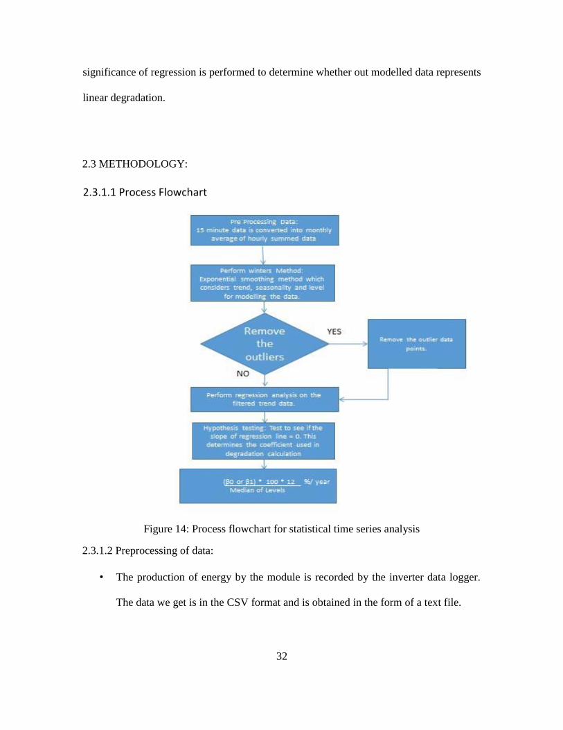
2.3.1.1 Process Flowchart ………………………………………………………. ……… 32

2.3.1.2 Preprocessing of Data: ………………………………………….. .................. 32

2.3.1.3 Modelling Data Using Time Series Methods: ……………………………....... 34

2.3.1.4 Winter’s Method: ……………………………………………………........... 35

2.3.1.5 Residual Analysis and Smoothers: …………………………………............ 36

2.3.1.6 Filtration of Outliers In The Trend Data: …………………………………. 37

2.3.1.7 Hypothesis Testing: ……………………………………………………………...39

2.3.1.8 Regression Analysis Performed on the Filtered Trend Data: ………………..40

2.3.2 Linearity Analysis Using Pmax Degradation in Hot Dry Climatic Condition..... 41

2.4 RESULTS AND DISCUSSION: ................................................................................ 43

2.4.1 MODEL CT.......................................................................................................... 43

2.4.1.1 Winters Method on the Preprocessed Data: …………………………………...43

2.4.1.2 Residual Analysis of the Noise Component: ………………………………….44

2.4.1.3 Unfiltered Trend Data: …………………………………………………. ...... 44

2.4.1.4 Filtered Trend Data: …………………………………………………. .......... 45

2.4.1.5 Hypothesis Testing: ……………………………………………................... 46

viii

CHAPTER Page

2.4.1.6 Calculation of Degradation Rate Per Year: ……………………………......... 46

2.4.2 Model G................................................................................................................ 47

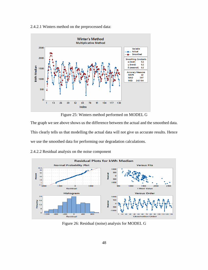
2.4.2.1 Winters Method on the Preprocessed Data: ………………………………...48

2.4.2.2 Residual Analysis on the Noise Component: ……………………………….48

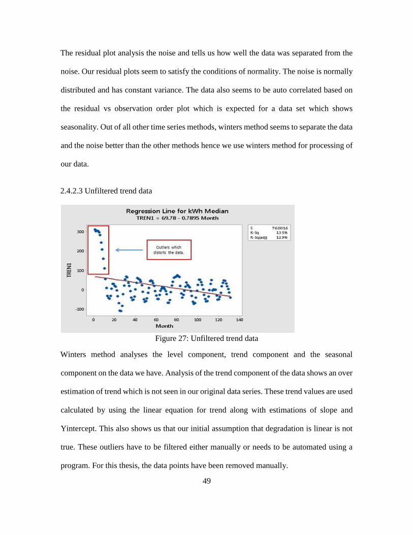
2.4.2.3 Unfiltered Trend Data ……………………………………............................49

2.4.2.4 Filtered Trend Data…………………………………………...........................50

2.4.2.5 Hypothesis Test of μ = 0 vs ≠ 0………………………………........................50

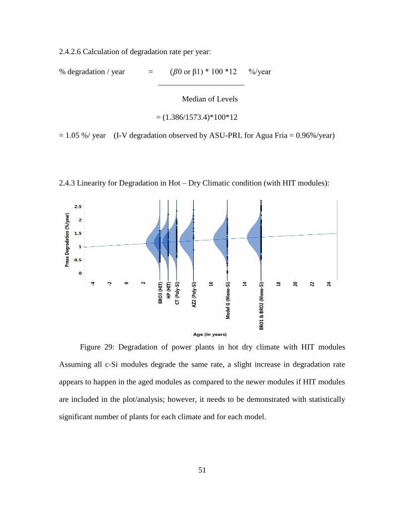
2.4.2.6 Calculation of Degradation Rate Per Year: ………………….......................51

2.4.3 Linearity for Degradation in Hot – Dry Climatic Condition (with HIT

modules): ....................................................................................................................... 51

2.4.4 Linearity for Degradation in Hot – Dry Climatic condition (without HIT

modules):........................................................................................................................ 52

2.5 CONCLUSION ......................................................................................................... 53

REFERENCES: ............................................................................................................. 55

APPENDIX

A COMPREHENSIVE PERFORMANCE ANALYSIS OF POWER PLANTS ........... 58

ix

LIST OF TABLES

Table Page

1. Defect Affecting Performance Parameters ..................................................................... 8

2. Severity ......................................................................................................................... 13

3. Occurence ..................................................................................................................... 13

4. Detection....................................................................................................................... 14

x

LIST OF FIGURES

Figure Page

1. Metric Definitions of Failures ................................................................................. 5

2. Visible and Invisible Defects Classification ........................................................... 7

3. I-V Data Format .................................................................................................... 15

4. Global RPN for Defects in MODEL J .................................................................. 16

5. Method to Detect Dominant Performance Parameter ........................................... 17

6. Classification of Defects Across Different Climatic Conditions .......................... 20

7. Classification of Defects with RPN Color Coordinated ....................................... 21

8. Defects Color Coordinated for Different Regions with RPN/Age ....................... 24

9. Dominant Defect Found in Hot and Dry Climatic Condition ............................... 25

10. Dominant Defects Found in Cold and Dry Climatic Conditions .......................... 26

11. Process Flowchart for Statistical Time Series Analysis ....................................... 33

12. Process of Smoothing the Data Set ....................................................................... 37

13. Analaysis of the Noise Component of Data .......................................................... 39

14. Unfiltered Trend Data ........................................................................................... 43

15. Graph of Preprocessed Data.................................................................................. 43

16. Winters’ Method Smoothed vs Actual Fit ............................................................ 44

xi

Figure Page

17. Residual (Noise) Analysis for Model AZ8 ........................................................... 44

18. Outliers in Trend Data .......................................................................................... 45

19. Preprocessed Data for MODEL G ........................................................................ 47

20. Winters Method Performed on MODEL G .......................................................... 47

21. Resdiual (Noise) Analysis for MODEL G ............................................................ 48

22. Unfiltered Trend Data ........................................................................................... 49

23. Filtered Trend Data ............................................................................................... 49

24. Degradation of Power Plants in Hot Dry Climate Including HIT Modules ......... 51

25. Degradation of Power Plants in the Hot and Dry Excluding HIT Modules ......... 51

1

PART 1: DEFECT ANALYSIS OF PV POWER PLANTS

1.1 INTRODUCTION

1.1.1 Background

In today’s Solar PV industry, mitigation of performance losses due to defects found in

power plants is of extreme importance. Based on the paper published by M.A.Quintana

et.al [1], Neelesh et.al [12] summarized that the degradation of photovoltaic modules in

the field could be due to the type of environment the modules are being exposed to,

manufacturing problems and quality of the design of the PV panels. The degradation

modes would cause the degradation of I-V parameters (Fill Factor, Open Circuit Voltage,

and Short Circuit Current) which eventually leads to the loss of the output power of a

module. This degradation could be caused by single or multiple modes of degradation.

The number of panels which are being installed every year seem to be increasing at an

exponential rate. This therefore creates a compulsive need to quantify the different risks

posed by these defects to the performance (degradation) of the power plants present in

different climatic conditions. This quantification of the risks associated to one particular

defect was determined using the Risk Priority Number (RPN) technique developed by

Shrestha et.al. [3]. Shravanthi et.al [15] and Vidhya et.al [14] further classified The RPN

is classified into three further categories: Safety RPN (S-RPN), Performance RPN

(PRPN) and Global RPN (G-RPN). In this thesis, we have focused particularly on global

RPN. Shrestha et.al [13] reported in his thesis that this method uses the Risk Priority

number Techniques to Rank the failure modes. The highest RPN number is assigned to

the failure mode which poses the worst risk and cause performance losses. RPN helps in

2

quantifying the performance losses (or degradation) caused due to a particular defect

found in the power plant. A database of RPN will help manufacturers and power plant

owners to determine the manufacturing or design inadequacies. Using this knowledge,

modules which are reliable to those particular defects can manufactured as reported by

Shrestha et.al [13]. Using the MATLAB code developed by Mathan et.al [4] which

automates the calculation of the RPN using a program based on mathematical formulas

for finding RPN, a database of RPN plots and Degradation rates correlated with defective

modules was created. This involved gathering the Visual inspection data gathered from

power plant visits which tells us the presence/absence of a defect in a module and this

data is correlated to the I-V data. These two file produce an output data correlation file

which quantifies the loss of performance of the module due to the defect present in it.

Using this data correlation file and RPN plots, a database consisting of the all the defects

found in the USA across power plants in different climatic conditions was created. Once

the database was created and every defect in each climatic condition had been listed, we

would be able to come up with a database for the dominant defects affecting performance

of power plants in each climatic conditions and their corresponding Risk priority numbers.

The goal of this part of the thesis is to:

• Develop an automated database for defects found in the power plants across

different climatic conditions and examine if the RPN is dictated by technology type,

climate and age.

• Create a database for all the defects by detecting, analyzing and summarizing the

defects found in different climatic conditions.

3

• Determining the dominant defect observed in each climatic condition across the

USA and assign a corresponding RPN number to reflect the possible financial risks

the dominant defects is posing to the power plants.

1.1.2 Statement of Problem:

Using the technology and data available at ASU-PRL, data for 14 power plants in the USA

was gathered and various output results were obtained using the MATLAB code developed

by Mathan et.al [4]. The defects were correlated with the rate of degradation of

performance parameters and Pmax degradation obtained for 14 power plants whereas the

RPN plots were obtained for 10 power plants since 4 power plants had no defects. With

such a wide database, we try to answer the pressing questions in today’s industry which are

stated below.

1. Establish the defects affecting the Pmax degradation for two weather conditions

such as hot and dry and cold and dry by statistically analyzing multiple power plants

and assigning RPN to each of the performance defects found in these power plants.

2. Determine dominant defects in each climatic condition and assigning an RPN to

quantify each defect so that manufacturers and investors can come up with climate

specific accelerated tests to mitigate the effects of dominant defects. This also

creates a possibility to also develop defect specific accelerated tests for the most

dominant defects which is independent of the climate.

1.1.3 Objective

Evaluation of a PV power plant and performing RPN analysis on the defects in PV power plant

used to be carried out manually. Manual evaluation is time consuming and involves lot of

4

manual labor to perform these analyses. In order to overcome this, it is better to automate the

process which was done by Mathan et.al [4], where a RPN program in MATLAB was created

to automatically calculate the Global RPN. Using this automated process and the vast amount

of data available at ASU-PRL, it is possible to come up with a database for the performance of

power plants and the defects affecting them in different weather conditions across the USA

along with the associated risk of the defect being provided by the RPN. It also helps PV power

plant owners to identify the modules with failures and understand the failure modes causing it.

This helps design climate specific accelerated tests to mitigate the effect of particular defects.

When multiple power plants in each weather condition is analyzed and the dominant failure

modes are determined, we would end up with a database which could be used by the power

plant owners to make decisions on the power plants (retain/sell/buy).

1.2 LITERATURE REVIEW

1.2.1 Safety, Reliability and Durability failures:

Tamizhmani et.al [5] defined failures as “If the PV modules are removed (or replaced) from

the field before the warranty period expires due to any type of failure, including power

drop beyond warranty limit, then those failures may be classified as hard failures. In other

words, all failures that qualify for warranty returns may be called a reliability failure. If the

performance of PV modules degrades but still meets the warranty requirements, then those

losses may be classified as soft losses or degradative losses. Toward the end of the

module’s life, multiple degradative mechanisms may develop and lead to wear-out failures

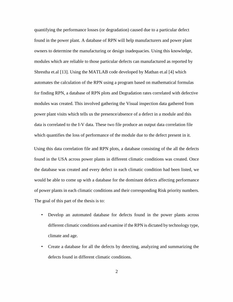
due to accelerated degradative losses”. Figure 1 shows the metric definitions for safety

failure, reliability failure, and durability loss.

5

Figure 1: metric definitions of failures

1.2.2 Defects/Failures found in PV Modules

Investors and power plant owners looking to buy power plants or thinking if they should

retain or sell the existing plant can make such decisions based on two designed parameters,

(1). Rate of degradation correlated to the Defects observed visually in the power plant with

their corresponding RPN. With the information obtained from these calculated parameters,

we can say if the power plant is healthy or not. We do this statistically by using the Risk

Priority Number program which can tell the investor/owner if the dominant defect observed

is harmful or not. Risk priority number (RPN) for each defect/failure is automatically

generated based on visual inspection spreadsheet (VI). Automation program package

developed by Mathan et.al [4] involves two major programs – one which is used to

calculate the global RPN and other is to find the modules with defects and their correlation

with IV parameters degradations. The goal of the project is to create a database for RPN

using the global RPN program (safety RPN + Performance RPN) for 10 power plants

6

evaluated by ASU-PRL. Investors can use this as a guide which tells them the dominant

defects in each weather condition and the defects observed in two weather conditions along

with the corresponding risks associated to those defects using the RPN for each defect.

Based on the information we obtain from RPN, the plant owners will be able to make

warrantee entitlements from the manufacturer and also to decide whether it would be

profitable to retain the power plant or not.

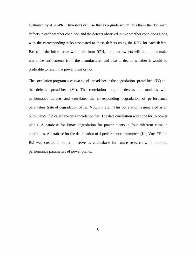
The correlation program uses two excel spreadsheets: the degradation spreadsheet (IV) and

the defects spreadsheet (VI). The correlation program detects the modules with

performance defects and correlates the corresponding degradation of performance

parameters (rate of degradation of Isc, Voc, FF, etc.). This correlation is generated as an

output excel file called the data correlation file. The data correlation was done for 15 power

plants. A database for Pmax degradation for power plants in four different climatic

conditions. A database for the degradation of 4 performance parameters (Isc, Voc, FF and

Rs) was created in order to serve as a database for future research work into the

performance parameters of power plants.

7

1.3 METHODOLOGY

1.3.1 Visible and invisible defects

Figure 2: Visible and invisible defects classification [Performance defects and safety failures

are listed elsewhere, [4]]

8

Janakeeraman et.al [27] analyzed the IV data collected from 8 different PV power plants

in Arizona to identify the IV parameters which are responsible for degradation of power

and correlated them with the defects/failures found in PV modules.

Umachandran et.al [12] correlated the visual defects found in power plants obtained from

5 different PV power plants in Arizona and New York with IV parameters to identify the

exact defect/failure which is liable for affecting the dominant IV parameter causing Pmax

degradation. In this thesis we try to classify these defects/failures as visible (to the naked

eye) or invisible (equipment need to find presence/absence of a particular defect).

Invisible defects are assigned with a high number for detectability as they are not visible

to the naked eye and the risk posed by such defects could be dangerous as it is easy to

overlook them when they might be causing high losses in performance. Such defects have

to be detected using sophisticated equipment such as I-V curve tracer, I-R camera or

circuit continuity detectors. Solder bond failures was one of the invisible defects which

contributes to huge losses in performance and needs to be detected using the I-V tracer.

Visible defects on the other hand are given a low number for detectability as they do not

require sophisticated equipment for detection and are visible to the naked eye. In this

thesis, a classification table classifying all the defects observed in PV modules as visible

and invisible, method to detect invisible defects and the corresponding performance

parameters affected was created which is shown below.

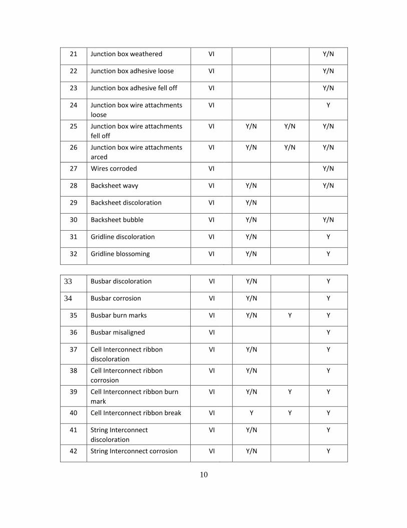
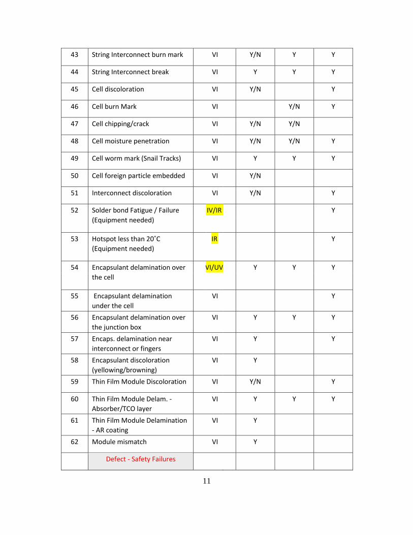
1.3.2 Performance parameter primarily expected to be affected by each defect

Power = Isc x Voc x FF

(VI=Visual; IV=I-V curve; IR=IR imaging; CC=Circuit Continuity;

UV=UV fluorescence); Yes (Y) = Affected; Yes/No (Y/N) = May be

affected

9

Table 1: Defect Affecting Performance Parameters

Defec

t # Defect – Performance Defect

Detectio

Method

VI/IV/IR/

C

n

C

Paramete

r

Affected:

Isc

Paramete

r

Affected:

Voc

Paramete

r

Affected:

FF

1 Front glass lightly soiled VI Y

2 Front glass heavily soiled VI Y

3 Front glass crazing VI Y

4 Front glass chip VI Y/N

5 Front glass milky discoloration VI Y

6 Rear glass crazing VI Y/N

7 Rear glass chipped VI Y/N

8 Edge seal delamination VI Y

9 Edge seal moisture penetration VI Y

10 Edge seal discoloration VI Y/N

11 Edge seal squeezed / pinched

out

VI Y/N

12 Frame bent VI Y/N

13 Frame discoloration VI Y/N

14 Frame adhesive degraded VI Y/N

15 Frame adhesive oozed out VI Y/N

16 Frame adhesive missing in areas VI Y/N

17 Bypass diode short circuit

(Equipment needed)

IV/IR/CC Y Y

18 Junction box lid loose VI Y/N

19 Junction box lid crack VI Y/N

20 Junction box warped VI Y/N

:

10

21 Junction box weathered VI Y/N

22 Junction box adhesive loose VI Y/N

23 Junction box adhesive fell off VI Y/N

24 Junction box wire attachments

loose

VI Y

25 Junction box wire attachments

fell off

VI Y/N Y/N Y/N

26 Junction box wire attachments

arced

VI Y/N Y/N Y/N

27 Wires corroded VI Y/N

28 Backsheet wavy VI Y/N Y/N

29 Backsheet discoloration VI Y/N

30 Backsheet bubble VI Y/N Y/N

31 Gridline discoloration VI Y/N Y

32 Gridline blossoming VI Y/N Y

33 Busbar discoloration VI Y/N Y

34 Busbar corrosion VI Y/N Y

35 Busbar burn marks VI Y/N Y Y

36 Busbar misaligned VI Y

37 Cell Interconnect ribbon

discoloration

VI Y/N Y

38 Cell Interconnect ribbon

corrosion

VI Y/N Y

39 Cell Interconnect ribbon burn

mark

VI Y/N Y Y

40 Cell Interconnect ribbon break VI Y Y Y

41 String Interconnect

discoloration

VI Y/N Y

42 String Interconnect corrosion VI Y/N Y

11

43 String Interconnect burn mark VI Y/N Y Y

44 String Interconnect break VI Y Y Y

45 Cell discoloration VI Y/N Y

46 Cell burn Mark VI Y/N Y

47 Cell chipping/crack VI Y/N Y/N

48 Cell moisture penetration VI Y/N Y/N Y

49 Cell worm mark (Snail Tracks) VI Y Y Y

50 Cell foreign particle embedded VI Y/N

51 Interconnect discoloration VI Y/N Y

52 Solder bond Fatigue / Failure

(Equipment needed)

IV/IR Y

53 Hotspot less than 20˚C

(Equipment needed)

IR Y

54 Encapsulant delamination over

the cell

VI/UV Y Y Y

55 Encapsulant delamination

under the cell

VI Y

56 Encapsulant delamination over

the junction box

VI

Y Y Y

57 Encaps. delamination near

interconnect or fingers

VI Y Y

58 Encapsulant discoloration

(yellowing/browning)

VI Y

59 Thin Film Module Discoloration VI Y/N Y

60 Thin Film Module Delam. -

Absorber/TCO layer

VI Y Y Y

61 Thin Film Module Delamination

- AR coating

VI Y

62 Module mismatch VI Y

Defect - Safety Failures

12

63 Front glass crack VI Y Y Y

64 Front glass shattered VI Y Y Y

65 Rear glass crack VI Y Y Y

66 Rear glass shattered VI Y Y Y

67 Frame grounding severe

corrosion

VI N

68 Frame grounding minor

corrosion

VI N

69 Frame major corrosion VI N

70 Frame joint separation VI N

71 Frame cracking VI Y/N N

72 Bypass diode open circuit

(Equipment needed)

IR/CC Y/N Y/N

73 Junction box crack VI Y/N Y

74 Junction box burn VI Y/N Y

75 Junction box loose VI Y/N Y

76 Junction box lid fell off VI Y/N Y

77 Wires insulation cracked /

disintegrated

VI Y

78 Wires burnt VI Y/N Y

79 Wires animal bites / marks VI Y

80 Backsheet peeling VI Y Y Y

81 Backsheet delamination VI Y Y Y

82 Backsheet burn mark VI Y Y Y

83 Backsheet crack /cut under cell VI Y

84 Backsheet crack /cut between

cells

VI Y

85 String Interconnect arc tracks VI Y/N Y

13

86 Hotspot over 20˚C (Equipment

needed)

IR Y Y Y

Figure 3: Visible and invisible defects classification [Performance defects and safety failures

are listed elsewhere, [4]]

1.3.3 Comprehensive Analysis of Power Plants:

Identifying the potential defects/failures that could occur in the field provides an insight

for the manufacturers. Using the defects database generated in this thesis, the industry

will be able to quantify safety and performance risks for these defects so that appropriate

accelerated tests to mitigate the effect of that particular defect can be developed.

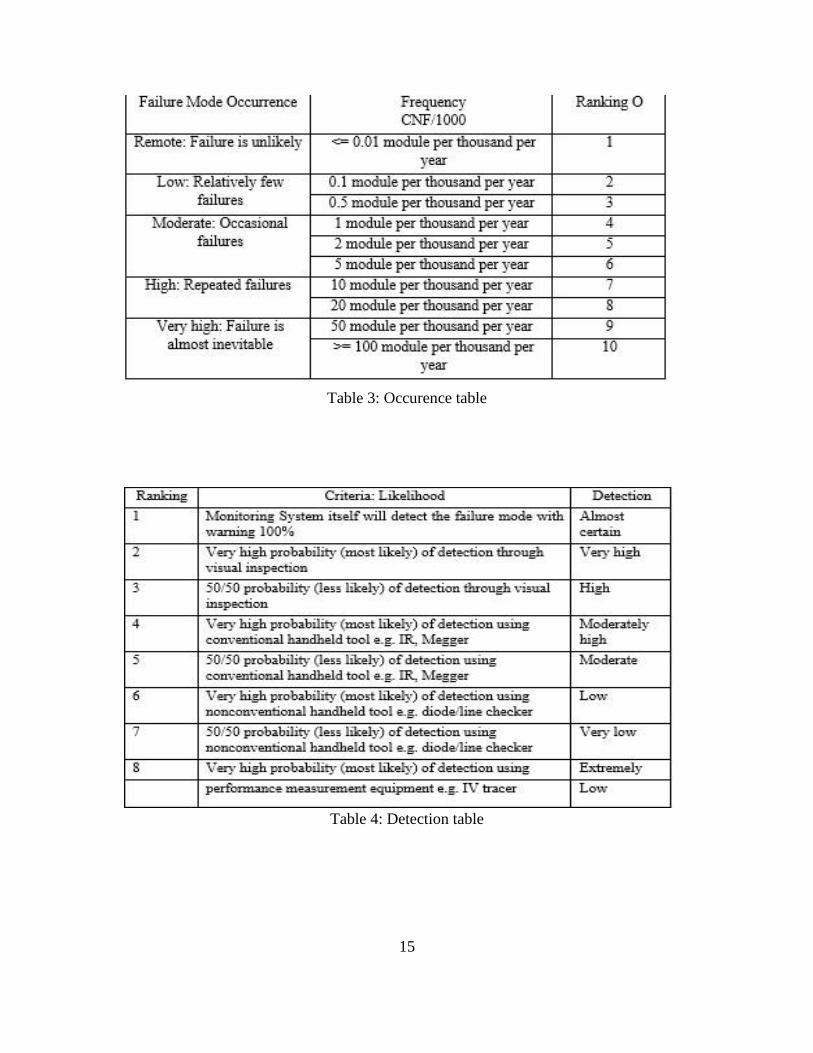
1.3.4 Risk Priority Number:

In part 1 of this project, the aim is to categorically determine the RPN for defects occurring

In 10 power plants around USA based on the occurrence, detectability and severity table

developed by Shrestha et.al [13] for the PV industry. Each of these power plants belong to

one of the 4 climatic conditions – Hot and Dry, Cold and Dry, Hot and Humid and

Temperate. For each of these power plants, every defect occurring in each of these power

plants has been assigned with a RPN number. Shrestha et.al [13] defines RPN, risk priority

number, as one of the approaches for quantification of the criticality of the failure mode as

indicated in IEC 60812 2006-01 Standard [8] and is given by

RPN = S * O * D

Where: S means Severity which is a measure of how strongly a system or a consumer is

affected due to the effect of the defect present.

14

O means Occurrence (or likelihood) which denotes how probable it is for the particular failure

mode to occur for a predetermined time interval

D means Detection which is an estimate of how easily the defect or the failure mode can be

identified before the failure reaches the customer. [13]

Using this equation as a formula, the program developed by Mathan et.al [4] calculates the

RPN based on Severity, occurrence and detection. The Severity table proposed by Shrestha

et.al [3] was modified by Mathan et.al [4] which has been used here. The occurrence and

detection table developed by Shrestha et.al. [3] has been shown below.

Table 2: Severity table

15

Table 3: Occurence table

Table 4: Detection table

16

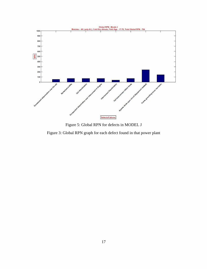
1.3.5 MATLAB Program input data:

The generation of RPN for 15 power plants is done using the MATLAB program developed

by Mathan et.al [4] and by using two forms as spreadsheet as the input: One is the defects

spreadsheet (IV Data) and other one is the degradation rate spreadsheet (VI). Both these

spreadsheets have to be in the exact format as shown below in order for it to run in the

MATLAB program.

Figure 4: I-V data format

The Degradation rate spreadsheet needs to be saved as IV data and the Defects spreadsheet

needs to be saved as VI. Saving these two spreadsheets by any other name will result is the

program not running. Once the data has been inputted in the form of 2 spreadsheets, the

global RPN program produces the RPN number for every defect. It also provides us with

an additional 5 graphs which helps us determine other characteristics related to RPN.

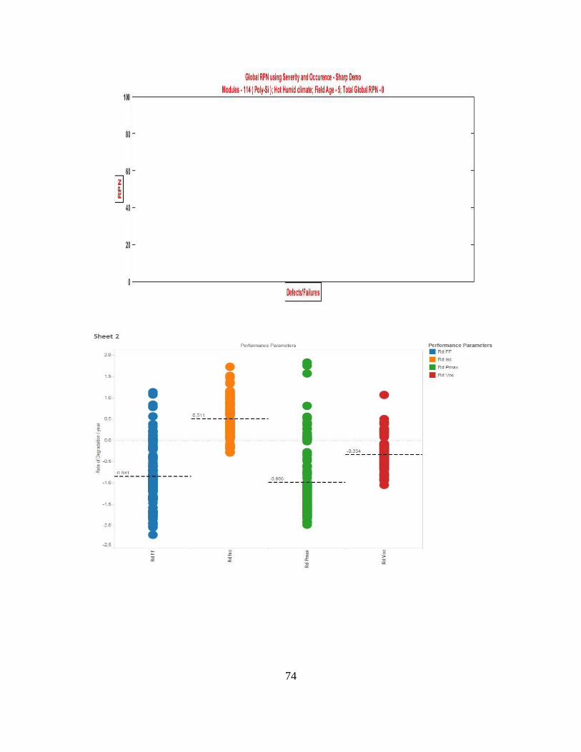
Below is the RPN plot generated for a particular power plant and based on this we generate

RPN for 15 power plants. In this thesis, we consider the global RPN plots shown below:

17

Figure 5: Global RPN for defects in MODEL J

Figure 3: Global RPN graph for each defect found in that power plant

18

1.3.8 Method to Detect the Dominant Defect in Each Power Plant

Figure 6: Method to detect dominant performance parameter

1.3.9 Generic dominant defects pie chart:

The usual pie chart’s which are published in the industry contain dominant defects found

in each climatic condition. However, these pie charts do not give an idea of the level of

risk associated to these dominant defects. In this part of the thesis, an attempt at

quantifying the level of risk associated to these defects found in different climatic

conditions by assigning a risk priority number to the dominant defects (figure (14) and

figure (15) in the results and discussion section). This way we can quantify the risk

associated to the dominant defect. Below we can see two such pie charts, figure 7 and

19

figure 8 published in [28] shows the dominant defects calculated in percentage as

compared to the total number of failures.

Figure 7: Generic pie chart showing percentage of each defect [28]

Figure 8: Generic dominant defect flowchart based on customer complaints [28]

20

1.4 RESULTS AND DISCUSSION

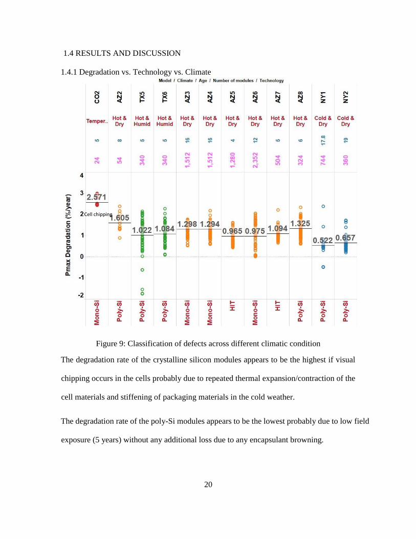
1.4.1 Degradation vs. Technology vs. Climate

Figure 9: Classification of defects across different climatic condition

The degradation rate of the crystalline silicon modules appears to be the highest if visual

chipping occurs in the cells probably due to repeated thermal expansion/contraction of the

cell materials and stiffening of packaging materials in the cold weather.

The degradation rate of the poly-Si modules appears to be the lowest probably due to low field

exposure (5 years) without any additional loss due to any encapsulant browning.

Cell chipping

21

In general, based on this plot, it can be concluded that the crystalline silicon modules degrade

in the following order: hot-dry > hot-humid >> cold-dry.

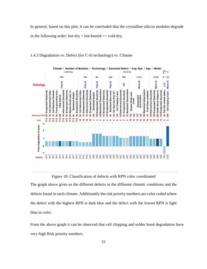
1.4.3 Degradation vs. Defect (for C-Si technology) vs. Climate

Figure 10: Classification of defects with RPN color coordinated

The graph above gives us the different defects in the different climatic conditions and the

defects found in each climate. Additionally the risk priority numbers are color coded where

the defect with the highest RPN is dark blue and the defect with the lowest RPN is light

blue in color.

From the above graph it can be observed that cell chipping and solder bond degradation have

very high Risk priority numbers.

22

Another major conclusion from this graph would be that the RPN of defects found in

HotDry weather condition is higher than the RPN for Cold-Dry and Hot-Humid. Also Hot-

Dry weather condition has a much wider variety of defects as compared to other climatic

conditions.

From this graph we can infer the order of RPN for different climatic conditions to be: Hot-

Dry > Cold-Dry >> Hot- Humid

The Hot-Humid climatic condition has less number of defects because the plants are only 5

years old.

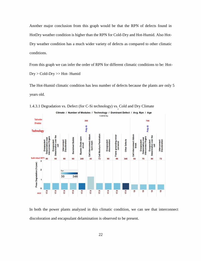
1.4.3.1 Degradation vs. Defect (for C-Si technology) vs. Cold and Dry Climate

In both the power plants analyzed in this climatic condition, we can see that interconnect

discoloration and encapsulant delamination is observed to be present.

23

We can also see a high RPN for other defects for NY2 as there were 6-8 defects with low

RPN values which were not occurring in any other power plant. It was determined that

these are not the dominant defects due to the low RPN they possess and were grouped

together as other defects.

1.4.3.2 Degradation vs. Defect (for C-Si technology) vs. Hot and Dry Climate

Thousands of modules in the hot dry climatic condition was analyzed and larger number of

defects were observed as compared to the other climatic conditions.

From the above graph, it is clearly visible that solder bond fatigue failure has the highest

RPN. Encapsulant discoloration seem to be happening in almost every power plant in the

hot dry climatic condition.

24

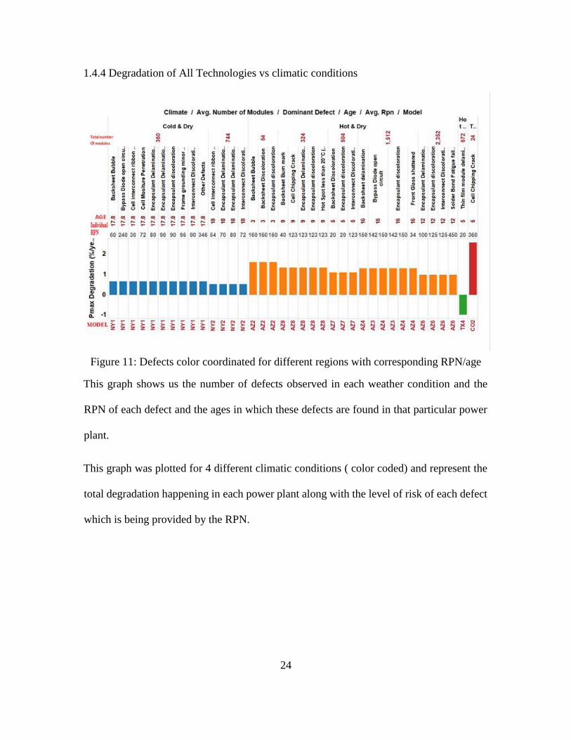
1.4.4 Degradation of All Technologies vs climatic conditions

Figure 11: Defects color coordinated for different regions with corresponding RPN/age

This graph shows us the number of defects observed in each weather condition and the

RPN of each defect and the ages in which these defects are found in that particular power

plant.

This graph was plotted for 4 different climatic conditions ( color coded) and represent the

total degradation happening in each power plant along with the level of risk of each defect

which is being provided by the RPN.

25

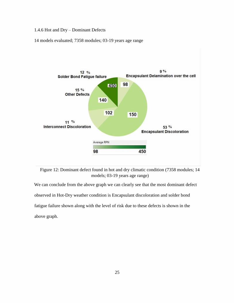
1.4.6 Hot and Dry – Dominant Defects

14 models evaluated; 7358 modules; 03-19 years age range

Figure 12: Dominant defect found in hot and dry climatic condition (7358 modules; 14

models; 03-19 years age range)

We can conclude from the above graph we can clearly see that the most dominant defect

observed in Hot-Dry weather condition is Encapsulant discoloration and solder bond

fatigue failure shown along with the level of risk due to these defects is shown in the

above graph.

26

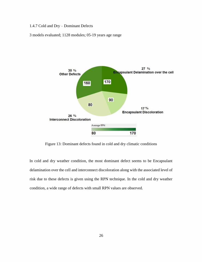
1.4.7 Cold and Dry – Dominant Defects

3 models evaluated; 1128 modules; 05-19 years age range

Figure 13: Dominant defects found in cold and dry climatic conditions

In cold and dry weather condition, the most dominant defect seems to be Encapsulant

delamination over the cell and interconnect discoloration along with the associated level of

risk due to these defects is given using the RPN technique. In the cold and dry weather

condition, a wide range of defects with small RPN values are observed.

27

1.5 CONCLUSION

In the first part, a detailed analysis on the performance or financial risk related to

each defect found in multiple PV power plants across various climatic regions of the USA

is presented by assigning a risk priority number (RPN). In this analysis it is determined

that the RPN for each plant is dictated by the technology type (crystalline silicon or thin-

film), climate and age. The PV modules aging between 3 and 19 years in four different

climates of hot-dry, hot-humid, cold-dry and temperate are investigated in this study.

Using an automated RPN program developed in a previous work at ASU-PRL and with

the vast amount data collected by ASU-PRL over several years, it was possible to

calculate the RPN for multiple power plants across varied weather conditions in the USA.

The automated MATLAB based RPN program also produces a data correlation file which

gives us the rate of degradation of each performance parameter and by using this

information one can pinpoint the dominant performance parameters (Voc, Isc and FF)

affected by each defect.

This study performed the defect correlation only for one parameter, power (Pmax).

Overall, based on the RPN analysis, the Pmax parameter is determined to be affected by

two dominant defects of encapsulant discoloration and solder bond defects across

multiple power plants in multiple climatic conditions. In some specific power plants, the

defects of cell chipping and bypass diode failure under open-circuit condition are

determined to have very high RPN values as compared to other defects. This study

recommends to extend this correlation analysis for the other performance parameters of

short-circuit current (Isc), open-circuit voltage (Voc) and fill factor (FF).

28

PART 2: DEGRADATION ANALYSIS OF PV POWER PLANTS

2.1 INTRODUCTION

Linearity in degradation is analyzed using 2 methods, namely, the I-V method and kWh

method. The I-V method involves going to the plant in person along with several equipment

(such as I-V curve tracer, thermocouples, reference cells, etc.) and calculating degradation

using the data collected from the mean median and worst performing strings within a 95%

confidence interval. In the I-V method, the annual Pmax degradation of 7538 crystalline

silicon modules of different ages present across 6 power plants in the hot and dry weather

condition is analyzed. The kWh method involves the statistical analysis performed on the

metered raw kWh data obtained from the inverter data logger which can be accessed

remotely from any location. This data consists of signal and noise components. Exponential

smoothers such as Winters’ method which is used for data which show seasonal variations.

These smoothers remove the noise from the data by taking the average of the current and

previous observations. Further, analysis of the noise (residual plot) will determine whether

the noise is random or not based on 4 conditions. If the 4 conditions are satisfied then the

noise is random and the data can be trusted. We make an assumption of linear degradation

and model the data to calculate degradation. Accurate values of degradation seems to imply

that our initial assumption that degradation is linear is correct for these two particular power

plants. Using these two methods and evaluation of thousands of modules, we could come

to a conclusion on the linearity of degradation in the hot dry condition.

29

2.1.1 Background:

In order to model the kWh data we obtain from the inverter, we need to first determine that

the components in the balance of system do not degrade because if they do degrade then it

could be contributing to the PV module degradation and we need to consider other

degradations in modelling kWh degradation. Hence we analyze different components in

the balance of system whether they fail or degrade. The components of the balance of

system usually fail at the end of their service life and do not degrade. Hence we statistically

model for the module degradation alone.

2.1.1.1 Balance of system and its components:

The balance of system encompasses all components of a photovoltaic system other than the

PV panels. This includes wiring, switches, mounting system, inverter and battery. In order

to model the kWh data we obtain from the inverter, we need to first determine that the

components in the balance of system do not degrade because if they do degrade then it

could be contributing the PV module degradation and we need to consider other

degradations in modelling kWh degradation. Hence we analyze different components in

the balance of system whether they fail or degrade.

• Inverter: Does not degrade over time. Performs throughout service life and fails.

• Mounting System: The single axis trackers being considered in the analysis here

does not have any degradation losses of PV module due to mounting. Neither is

there any degradation due to batteries as these modules are connected to the grid.

30

Since almost all the components in the balance of system fail and none of them

degrade, we attribute the trends observed in the kWh graphing to be due to the module

degradation only.

Hence we model the data for variations in module degradation. This is done using the

winter’s method in MINITAB.

2.1.2 Statement of problem:

Reason for using statistical technique’s in data processing:

The data obtained by ASU-PRL is collected every 15 minutes and spans over 8 years of

module’s operation. In order to streamline the data processing and do it in a shorter time

and a highly automated format with minimal manual filtration of outliers, we need to

statistically model the data using time series techniques such as winter’s method. The goal

of this part of the thesis is to determine if degradation in the hot dry climatic condition is

linear or nonlinear. We try to answer the question of linearity based on 2 established

methods in the industry.

2.1.3 Objective

The degradation rate is a key parameter used by the PV module manufacturers to

determine their warranty period and the system owners to predict the energy production

and calculate the levelized cost of energy (LCOE). The PV industry typically utilizes

three different methods to determine the degradation rate and they are: I-V method,

performance ratio (PR) method and performance index (PI) method. The I-V method is

ideal but it is a labor and cost intensive method. Also, this method requires complete

shutdown of the power plant during I-V measurements. The PR method accounts for

31

YOY (year-over-year) insolation variation measurements on a daily, hourly and monthly

basis; however, this method requires insolation data which is accurate from a ground

mounted weather station. The PI method accounts for all sorts of YOY variations

including insolation, temperature, soiling, angle of incidence, BOS losses etc.; however,

again, this method requires accurate weather data. This thesis focuses on a fourth method

called “metered kWh” method. This method does not require any weather data and all it

requires is the metered kWh data. Only a select few research groups have explored this

method as the degradation rates determined by this method are often inaccurate due to

large number of outliers caused by variations in the environmental conditions including

insolation and in the installation conditions including shading. In this thesis, we use this

method to determine linearity and also the accurate degradation of power plants.

2.2 LITERATURE REVIEW:

The time series data which we model in this thesis consists of both cyclic patterns and

seasonal patterns and such data cannot be successfully modeled using basic polynomial

models. Several approaches are available for the analysis of such data. In this chapter we

will discuss exponential smoothing techniques that can be used in modeling seasonal time

series. This thesis focuses mostly on the Winters’ method introduced by Holt [ 1957] and

Winters’ [ 1960], where a seasonal adjustment is performed to the fitted linear trend

model as described in “Introduction to Time Series analysis and forecasting” (Douglas C.

Montgomery, Cheryl L.Jennings and Murat Kulahci, 2008) [26]. Once the trend data is

modelled regression analysis is performed on the data. The hypothesis test for

32

significance of regression is performed to determine whether out modelled data represents

linear degradation.

2.3 METHODOLOGY:

2.3.1.1 Process Flowchart

Figure 14: Process flowchart for statistical time series analysis

2.3.1.2 Preprocessing of data:

• The production of energy by the module is recorded by the inverter data logger.

The data we get is in the CSV format and is obtained in the form of a text file.

33

• This CSV file is converted into excel column format as shown below. This is done

with the help of an excel tool called text to columns.

• The data obtained in the data logger records data for every 15 minutes throughout

the operation of the module. The energy output is in the form of kW and kWh. For

this thesis, the kWh data has been considered as we are only interested the hourly,

monthly and yearly energy production.

• The 15 minute data obtained is converted into hourly energy using the filtration tool

in excel. The hourly kWh data needs to be preprocessed using excel before

statistical analysis (processing) can be done on the data.

• The converted hourly kWh data is further tweaked and converted into summed

daily data where each day (each data point) is the summation of the data produced

every 24 hours i.e. the hourly data. This is done with the help of an excel tool called

the pivot table.

• The daily data obtained is finally converted into monthly data (one data point per

month). This daily summed data for each day in a month is averaged for each

month. This data is the daily summed data averaged for each month. Therefore we

end up with 12 data points per month. The Graph for preprocessed kWh energy

produced during the plants operating lifetime is shown below.

34

Figure 18: Graph of preprocessed data

2.3.1.3 Modelling data via time series methods:

The kWh data considered for the thesis is strongly affected by the seasonal variation. One

of the most important parameters of module performance, which is, irradiance varies

based on season. This directly alters the output data, i.e. kWh data and hence has to be

modeled for seasonal variations.

35

2.3.1.4 Winter’s Method:

Figure 15: The process of smoothing a dataset [26]

The Holt-Winters method is made of three components used for modelling — one for the

linear trend component Lt, and one for the seasonal component denoted by St and the error

component which has a mean around zero and a constant variance as described in

Montgomery et al. [26]. The Winters’ method takes into consideration the level, seasonal and

trend estimates into consideration and models the data. For both the power plants considered in

this thesis, we focus more on the trend and level estimates produced by the winter’s method.

36

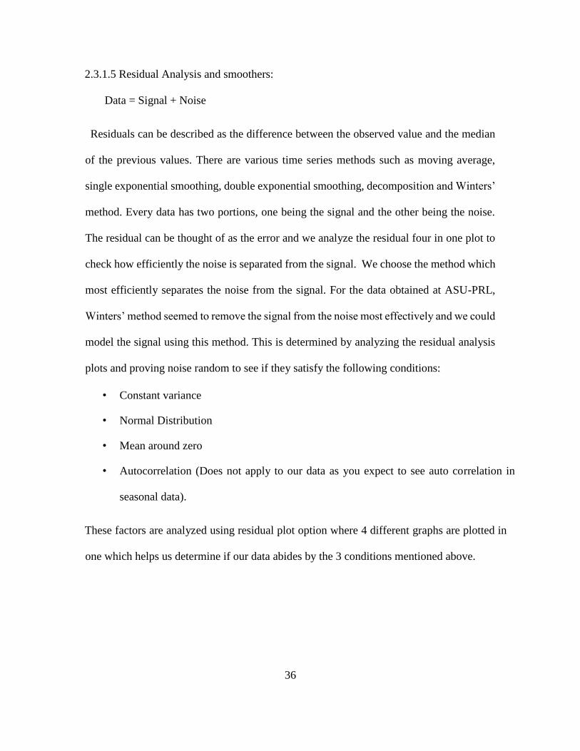
2.3.1.5 Residual Analysis and smoothers:

Data = Signal + Noise

Residuals can be described as the difference between the observed value and the median

of the previous values. There are various time series methods such as moving average,

single exponential smoothing, double exponential smoothing, decomposition and Winters’

method. Every data has two portions, one being the signal and the other being the noise.

The residual can be thought of as the error and we analyze the residual four in one plot to

check how efficiently the noise is separated from the signal. We choose the method which

most efficiently separates the noise from the signal. For the data obtained at ASU-PRL,

Winters’ method seemed to remove the signal from the noise most effectively and we could

model the signal using this method. This is determined by analyzing the residual analysis

plots and proving noise random to see if they satisfy the following conditions:

• Constant variance

• Normal Distribution

• Mean around zero

• Autocorrelation (Does not apply to our data as you expect to see auto correlation in

seasonal data).

These factors are analyzed using residual plot option where 4 different graphs are plotted in

one which helps us determine if our data abides by the 3 conditions mentioned above.

37

Figure 16: Analysis of the noise component of the data

• The frequency vs residual plot tells if our data is normally distributed or skewed.

• The percent vs residual plot tells us if our mean is distributed around zero or not.

• The residual vs fitted value plot tells us if our data has a constant variance or not.

• The residual vs observation graph tells us if the data is independent or auto correlated.

Based on analysis of these plot we can determine how well the noise is separated from the data.

Hence analysis of residual plots becomes important.

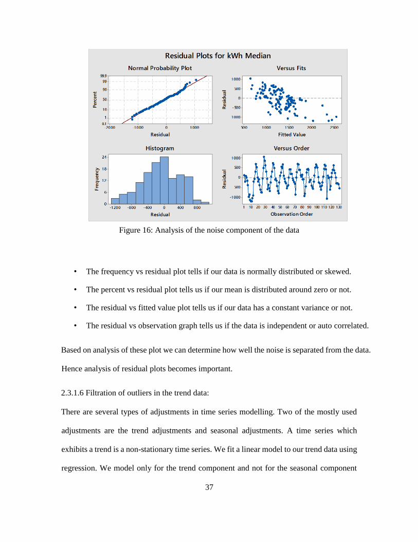
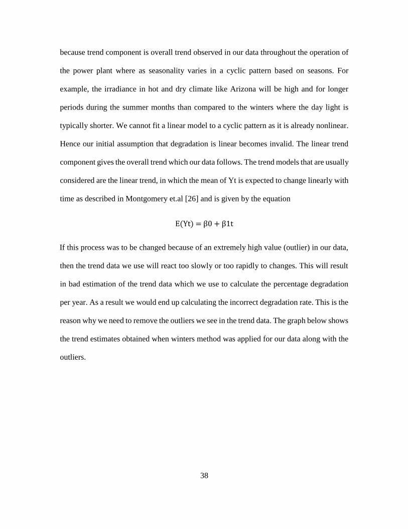
2.3.1.6 Filtration of outliers in the trend data:

There are several types of adjustments in time series modelling. Two of the mostly used

adjustments are the trend adjustments and seasonal adjustments. A time series which

exhibits a trend is a non-stationary time series. We fit a linear model to our trend data using

regression. We model only for the trend component and not for the seasonal component

38

because trend component is overall trend observed in our data throughout the operation of

the power plant where as seasonality varies in a cyclic pattern based on seasons. For

example, the irradiance in hot and dry climate like Arizona will be high and for longer

periods during the summer months than compared to the winters where the day light is

typically shorter. We cannot fit a linear model to a cyclic pattern as it is already nonlinear.

Hence our initial assumption that degradation is linear becomes invalid. The linear trend

component gives the overall trend which our data follows. The trend models that are usually

considered are the linear trend, in which the mean of Yt is expected to change linearly with

time as described in Montgomery et.al [26] and is given by the equation

E(Yt) = β0 + β1t

If this process was to be changed because of an extremely high value (outlier) in our data,

then the trend data we use will react too slowly or too rapidly to changes. This will result

in bad estimation of the trend data which we use to calculate the percentage degradation

per year. As a result we would end up calculating the incorrect degradation rate. This is the

reason why we need to remove the outliers we see in the trend data. The graph below shows

the trend estimates obtained when winters method was applied for our data along with the

outliers.

39

Figure 17: Unfiltered trend data

The initial points which distort our data were removed and regression analysis was

performed on the new filtered trend data. It can also be observed that the linear regression

equation obtained gives an extremely high coefficient value. When we use such a value for

calculating degradation, the value which we obtain will be out of bounds and nowhere close

to the correct value of % degradation per year. Further it also falsely leads us to believe

that the degradation seems nonlinear.

2.3.1.7 Hypothesis testing:

Hypothesis testing is performed on the filtered trend data after removing outliers to see if

the slope of the regression line is linear or not. This is of extreme importance because, if

we find out that the slope = 0, then our coefficient used in the equation used for

calculating percentage degradation per year changes from slope to y-intercept.

Hypothesis testing performed by hypothesizing if the slope value is 0 or not. This is done

by assuming the null hypothesis µ0 = 0. This means we basically assume the slope of the

40

regression line to be 0. Once we perform hypothesis testing, we look at the results and

summary table to make a decision on the data that we have obtained. Value of interest is

the p-value where p stands for probability. If the value is greater than 0.05 (i.e. 1-95%

CI), then it means the slope of the regression line is zero and our assumption that

degradation is linear is correct.

2.3.1.8 Regression analysis performed on the filtered trend data:

Accurate results of % degradation per year determine that our initial assumption that the

degradation is linear is true. This is of extreme importance as the end goal of this part of

the thesis is to determine the linearity in degradation. This is calculated by using the

formula:

(β0 or β1) 100 12 %/year

Median of levels

β0 = y intercept β1

= slope.

In our case, for the filtered trend data, the slope of the regression line determines the

coefficient used in the calculation of degradation. We perform hypothesis testing on the

slope of the regression line and hypothesize the slope to be 0, i.e., β0 = 0. A high p-value

indicates that our initial assumption that the slope is zero is correct. In such a case our y

intercept β1 used in the calculation of degradation. Degradation values for 2 power plants

were observed to be within ±0.09 compared to the degradation calculated using the I-V

41

method. Hence our initial assumption that the degradation is linear is true for these two

power plants in the hot dry weather condition.

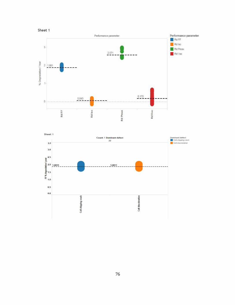
2.3.2 Linearity analysis using Pmax degradation in hot dry climatic condition

The IV database for 15 power plants is basically the data required to calculate performance

degradation. This data was obtained through field testing. I-V curves were collected for

individual modules for the best, median and worst strings of the whole plant. The

performance of the string as a whole was initially tested and the best median and worst

strings were chosen. From these selected strings individual modules were tested. The data

was translated to standard test conditions: STC (25°C, 1000W/m2).

Figure 18: ASU-PRL power plant evaluation procedure

Visual Inspection data of these modules were obtained using visual inspection checklist

modified by ASU-PRL based on the one developed by NREL [16]. Using the degradation

data obtained for 6 such power plants in the hot-dry weather condition, a statistical

42

determination on whether degradation is linear or nonlinear can be made. This will directly

impact the leveled cost of Estimation (LCOE) for PV modules. We try to check if the Pmax

degradation per year is linear or not based on the analysis of power plants having different

ages. We plot the Pmax degradation rate per year (Y- axis) versus time (age – X axis). We

try to see if the Pmax degradation rates of differently aged power plants fit the linear model.

43

2.4 RESULTS AND DISCUSSION:

2.4.1 MODEL CT

R² = 0.042

kWh Median

Figure 19: Preprocessed data for MODEL CJ

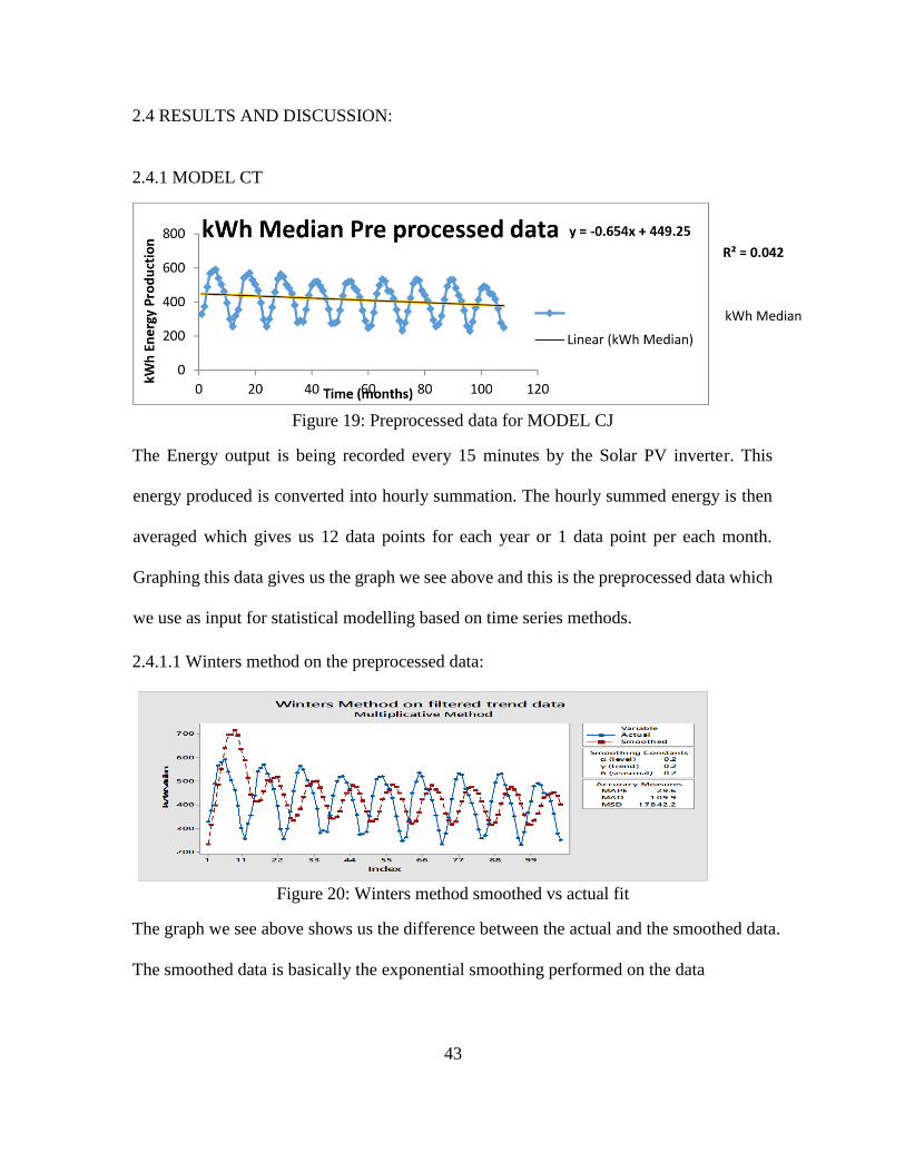
The Energy output is being recorded every 15 minutes by the Solar PV inverter. This

energy produced is converted into hourly summation. The hourly summed energy is then

averaged which gives us 12 data points for each year or 1 data point per each month.

Graphing this data gives us the graph we see above and this is the preprocessed data which

we use as input for statistical modelling based on time series methods.

2.4.1.1 Winters method on the preprocessed data:

Figure 20: Winters method smoothed vs actual fit

The graph we see above shows us the difference between the actual and the smoothed data.

The smoothed data is basically the exponential smoothing performed on the data

44

2.4.1.2 Residual analysis of the noise component

Figure 21: Residual (noise) analysis for MODEL AZ8

The residual plot analysis the noise and tells us how well the data was separated from the

noise. Our residual plots seem to satisfy the conditions of normality. The noise is normally

distributed and has constant variance. The data also seems to be auto correlated based on

the residual vs observation order plot which is expected for a data set which shows

seasonality. Out of all other time series methods, winters method seems to separate the data

and the noise better than the other methods hence we use winters method for processing of

our data.

2.4.1.3 Unfiltered trend data

Figure 22: Outliers in the trend data

45

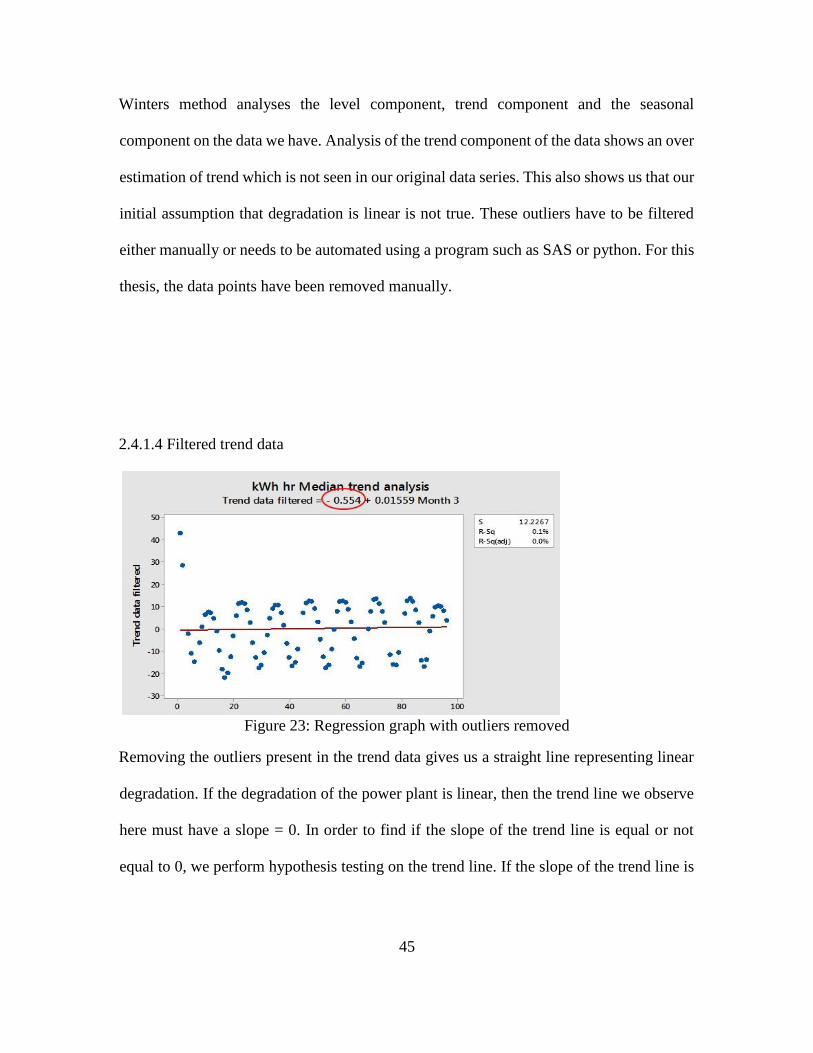
Winters method analyses the level component, trend component and the seasonal

component on the data we have. Analysis of the trend component of the data shows an over

estimation of trend which is not seen in our original data series. This also shows us that our

initial assumption that degradation is linear is not true. These outliers have to be filtered

either manually or needs to be automated using a program such as SAS or python. For this

thesis, the data points have been removed manually.

2.4.1.4 Filtered trend data

Figure 23: Regression graph with outliers removed

Removing the outliers present in the trend data gives us a straight line representing linear

degradation. If the degradation of the power plant is linear, then the trend line we observe

here must have a slope = 0. In order to find if the slope of the trend line is equal or not

equal to 0, we perform hypothesis testing on the trend line. If the slope of the trend line is

46

0, then the Y intercept seen in the linear equation becomes the new slope which will be

used in the formula for the calculation of degradation.

2.4.1.5 Hypothesis testing:

Test of μ = 0 vs ≠ 0

Variable N Mean StDev SE Mean 95% CI T P

Trend removed for outlier 121 -1.79 42.46 3.86 (-9.43, 5.85) -0.46 0.874

When we perform hypothesis test, we hypothesize the slope of the regression line to be 0.

The P-value which is the probability of our hypothesis being true. Here we see that the p

value = 0.874. This means that there is an 87.4% probability that our hypothesis is correct,

or in other words, the slope of the regression line obtained after removing the outliers is 0.

Since the slope of the line is 0, the Y-intercept obtained in the regression equation becomes

the new slope which will be used in the formula to calculate the degradation.

2.4.1.6 Calculation of degradation rate per year:

% degradation / year = (𝛽0 or β1) * 100 *12 %/year

Median of Levels

Degradation rate (%/year) = (β0/ median of levels)*100*12

(1.386/1573.4)*100*12

= -1.34 %/ year (I-V degradation observed by ASU-PRL for

Tempe Warehouse = 1.41%/year).

47

2.4.2 Model G

Figure 24: Preprocessed data for MODEL G

The Energy output is being recorded every 15 minutes by the Solar PV inverter. This energy

produced is converted into hourly summation. The hourly summed energy is then averaged

which gives us 12 data points for each year or 1 data point per each month. Graphing this

data gives us the graph we see above and this is the preprocessed data which we use as

input for statistical modelling based on time series methods.

48

2.4.2.1 Winters method on the preprocessed data:

Figure 25: Winters method performed on MODEL G

The graph we see above shows us the difference between the actual and the smoothed data.

This clearly tells us that modelling the actual data will not give us accurate results. Hence

we use the smoothed data for performing our degradation calculations.

2.4.2.2 Residual analysis on the noise component

Figure 26: Residual (noise) analysis for MODEL G

49

The residual plot analysis the noise and tells us how well the data was separated from the

noise. Our residual plots seem to satisfy the conditions of normality. The noise is normally

distributed and has constant variance. The data also seems to be auto correlated based on

the residual vs observation order plot which is expected for a data set which shows

seasonality. Out of all other time series methods, winters method seems to separate the data

and the noise better than the other methods hence we use winters method for processing of

our data.

2.4.2.3 Unfiltered trend data

Figure 27: Unfiltered trend data

Winters method analyses the level component, trend component and the seasonal

component on the data we have. Analysis of the trend component of the data shows an over

estimation of trend which is not seen in our original data series. These trend values are used

calculated by using the linear equation for trend along with estimations of slope and

Yintercept. This also shows us that our initial assumption that degradation is linear is not

true. These outliers have to be filtered either manually or needs to be automated using a

program. For this thesis, the data points have been removed manually.

50

2.4.2.4 Filtered trend data

Figure 28: Filtered trend data

Removing the outliers present in the trend data gives us a straight line representing linear

degradation. If the degradation of the power plant is linear, then the trend line we observe

here must have a slope = 0. In order to find if the slope of the trend line is equal or not

equal to 0, we perform hypothesis testing on the trend line. If the slope of the trend line is

0, then the Y intercept seen in the linear equation becomes the new slope which will be

used in the formula for the calculation of degradation.

2.4.2.5 Hypothesis Test of μ = 0 vs ≠ 0

Variable N Mean StDev SE Mean 95% CI T P

Trend removed for outlier 121 -1.79 42.46 3.86 (-9.43, 5.85) -0.46 0.644

When we perform hypothesis test, we hypothesize the slope of the regression line to be 0.

The P-value which is the probability of our hypothesis being true. Here we see that the p

value = 0.644. This means that there is a 64.4% probability that our hypothesis is correct,

or in other words, the slope of the regression line obtained after removing the outliers is 0.

Since the slope of the line is 0, the Y-intercept obtained in the regression equation becomes

the new slope which will be used in the formula to calculate the degradation.

51

2.4.2.6 Calculation of degradation rate per year:

% degradation / year = (𝛽0 or β1) * 100 *12 %/year

Median of Levels

= (1.386/1573.4)*100*12

= 1.05 %/ year (I-V degradation observed by ASU-PRL for Agua Fria = 0.96%/year)

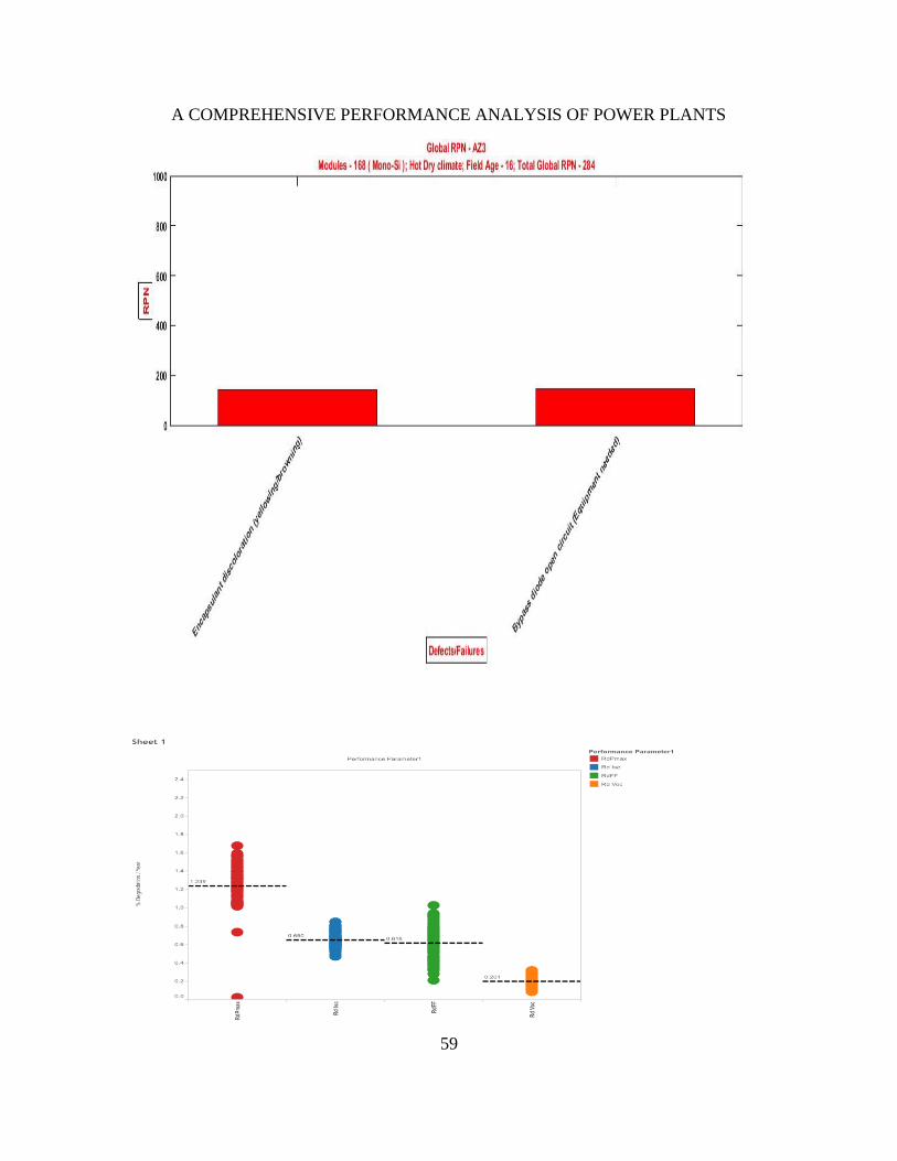
2.4.3 Linearity for Degradation in Hot – Dry Climatic condition (with HIT modules):

Figure 29: Degradation of power plants in hot dry climate with HIT modules

Assuming all c-Si modules degrade the same rate, a slight increase in degradation rate

appears to happen in the aged modules as compared to the newer modules if HIT modules

are included in the plot/analysis; however, it needs to be demonstrated with statistically

significant number of plants for each climate and for each model.

52

2.4.4 Linearity for Degradation in Hot – Dry Climatic condition (without HIT modules):

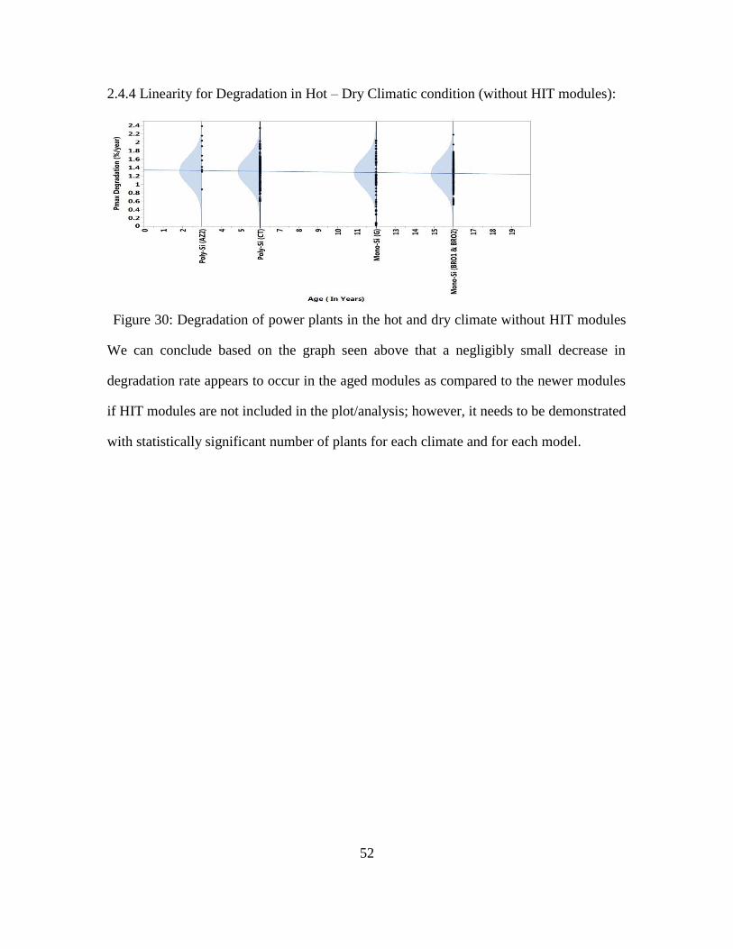
Figure 30: Degradation of power plants in the hot and dry climate without HIT modules

We can conclude based on the graph seen above that a negligibly small decrease in

degradation rate appears to occur in the aged modules as compared to the newer modules

if HIT modules are not included in the plot/analysis; however, it needs to be demonstrated

with statistically significant number of plants for each climate and for each model.

53

2.5 CONCLUSION

In the second part, a statistical degradation analysis is performed to determine if the

degradation rates are linear or not in the power plants exposed in a hot-dry climate for the

crystalline silicon technologies. This linearity degradation analysis is performed using the

data obtained through two methods: current-voltage method; metered kWh method.

For the current-voltage method, the annual power degradation data of hundreds of

individual modules in six crystalline silicon power plants of different ages is used. This

method involves going to the plant in person along with several equipment (such as I-V

curve tracer, thermocouples, reference cells, etc.). In this method, the best, median and

worst strings are statistically selected, and the I-V curves are performed on the modules

from the statistically selected best, median and worst strings. This process takes several

days to come up with a value for degradation rate for each plant depending on the size of

the plant. This preliminary study, based on four plants data obtained in a hot-dry climate,

appears to indicate that the crystalline silicon modules in hot-dry climate degrade linearly

with respect to time.

For the metered kWh method, the hourly kWh data secured from two powers plant

was used. This method, in principle, should consume less amount of time to determine the

degradation rate as it does not involve test personnel going to the PV plant sites.

However, the metered kWh data typically consists of the signal and noise components.

So, removing noise component on the degradation rate determination becomes critical.

Smoothers remove the noise component from the data by taking the average of the

current and the previous observations. Once this is done, a residual plot analysis of the

error component is performed to determine the noise was successfully separated from the

54

data by proving the noise is random. A residual plot analysis using Winters’ statistical

method is performed for two crystalline silicon plants of different ages in a hot-dry

climate. This analysis also appears to indicate that the degradation in hot-dry climate for

the crystalline silicon modules is linear. It is important to note that this linearity analysis

and conclusion have been done based on only a limited number of power plants.

Therefore, it is recommended to extend this study to more number of power plants in

diverse climatic conditions for different technologies. This entire procedure could be

automated using some software such as SAS or Python.

55

REFERENCES:

1) M. A. Quintana, D. L. King, T. J. McMohan, and C. R. Osterwald, “Commonly observed

degradation in field-aged photovoltaic modules,” 29th IEEE Photovoltaic Specialists

Conference, New Orleans, LA, USA, 2002, pp. 1436–1439

2) D. C. Jordan and S. R. Kurtz, “Photovoltaic Degradation Rates — An Analytical

Review, NREL/JA-5200-51664, June 2012

3) S. Shrestha, J. Mallineni, K. Yedidi, B. Knisely, S. Tatapudi, J. Kuitche, and G.

TamizhMani, “Determination of Dominant Failure Modes Using FMECA on the Field

Deployed c-Si Modules Under Hot-Dry Desert Climate”, IEEE Journal of Photovoltaics,

vol.5, no.1, pp.174-182, Jan. 2015.

4) Mathan Kumar Moorthy, “Automation of Risk Priority Number Calculation of

Photovoltaic Modules and Evaluation of Module Level Power Electronics” MS Thesis,

Arizona State University, December 2015.

5) J. Kuitche and G. TamizhMani, “Accelerated Lifetime Testing of Photovoltaic

Modules”.

6) M. A. Quintana, D. L. King, T. J. McMohan, and C. R. Osterwald, “Commonly observed

degradation in field-aged photovoltaic modules,” 29th IEEE Photovoltaic Specialists

Conference, New Orleans, LA, USA, pp. 1436–1439, 2002.

7) Source- en.wikipedia.org/wiki/Balance_of_system.

8) Analysis Techniques for System Reliability: Procedure for Failure Mode and Effects

Analysis (FMEA), IEC Std. 60812, 2006

9) Y. Xue, K. C. Divya, G. Griepentrog, M. Liviu, S. Suresh, and M. Manjrekar, "Towards

Next Generation Photovoltaic Inverters," IEEE Energy Conversion Congress and

Exposition (ECCE), 2011.

56

(10) W. Bower and D. Ton, "Summary Report on the DOE High-tech Inverter Workshop,"

DOE Office of Energy Efficiency and Renewable Energy, 2005.

(11) http://rredc.nrel.gov/solar/calculators/pvwatts/system.html

(12) N. Umachandran, J. Kuitche, G. TamizhMani, "Statistical Methods to Determine

Dominant Degradation Modes of Fielded PV Modules", IEEE PVSC, 2015.

13) Sanjay Shrestha,”Determination of Dominant Failure Modes using Combined

Experimental and Statistical Method to Calculate Degradation Rates”,MS Thesis, Arizona

State University, 2013,(repository.asu.edu).

(14) V. Rajasekar, “Indoor Soiling Method and Outdoor Statistical Risk Analysis of

Photovoltaic Power Plants”, MS Thesis, Arizona State University, 2014

(repository.asu.edu).

(15) S.Boppana, “Outdoor Soiling Loss Characterization and Statistical Risk Analysis of

Photovoltaic Power Plants”, MS Thesis, Arizona State University, 2014

(repository.asu.edu).

(16) C. E. Packard, J. H. Wohlegemuth, and S. R. Kurtz, “Development of a visual inspection

data collection tool for evaluation of fielded PV module condition,” Nat. Renew. Energy

Lab., Golden, CO, USA, Tech. Rep. NREL/TP-5200-56154, Aug. 2012.

(17) https://en.wikipedia.org/wiki/Errors_and_residuals.

(18) http://www.dfrsolutions.com/uploads/courses/SPI2012.pdf

(20) W. Bower and D. Ton, "Summary Report on the DOE High-tech Inverter Workshop,"

DOE Office of Energy Efficiency and Renewable Energy, 2005.

(21) http://rredc.nrel.gov/solar/calculators/pvwatts/system.html

(25) https://www.otexts.org/fpp/7/5

57

(26) Douglas C. Montgomery, Cheryl L.Jennings and Murat Kulahci, “Introduction to

time series analysis and forecasting”, Wiley Series in Probability and Statistics,2008.

(27) J. Mallineni, B. Knisely, K. Yedidi, S. Tatapudi, J. Kuitche and G. TamizhMani,

"Evaluation of 12-Year Old PV Power Plant in Hot – Dry Desert Climate: Potential

Use of Field Failure Metrics for Financial Risk Calculation", 40th IEEE Photovoltaic

Specialists Conference, pp. 3366 – 3371, 2014.

(28) Marc Köntges, Sarah Kurtz, Corinne Packard, Ulrike Jahn, Karl A. Berger, “Review of

Failures of photovoltaic modules”, Report IEA-PVPS T13-01:2014, Photovoltaic

Power system program.

58

APPENDIX A

DATA COLLECTED MAY 1998 - MAY 2014

59

A COMPREHENSIVE PERFORMANCE ANALYSIS OF POWER PLANTS

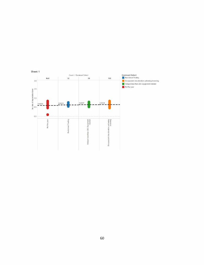
60

61

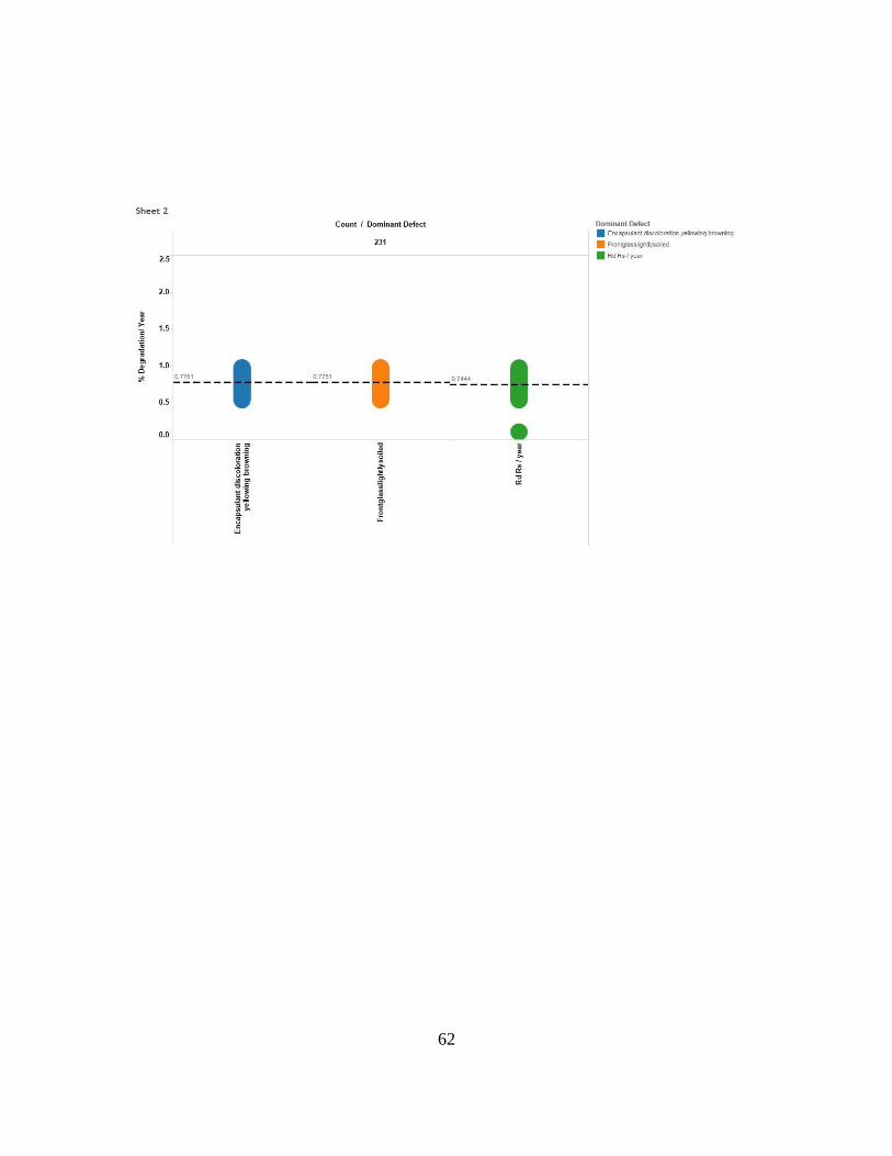
62

63

64

65

AZ7 RPN

66

High series resistance because HIT cells uses an Encapsulant different

from EVA.

67

AZ8 Affected Performance Parameter

68

69

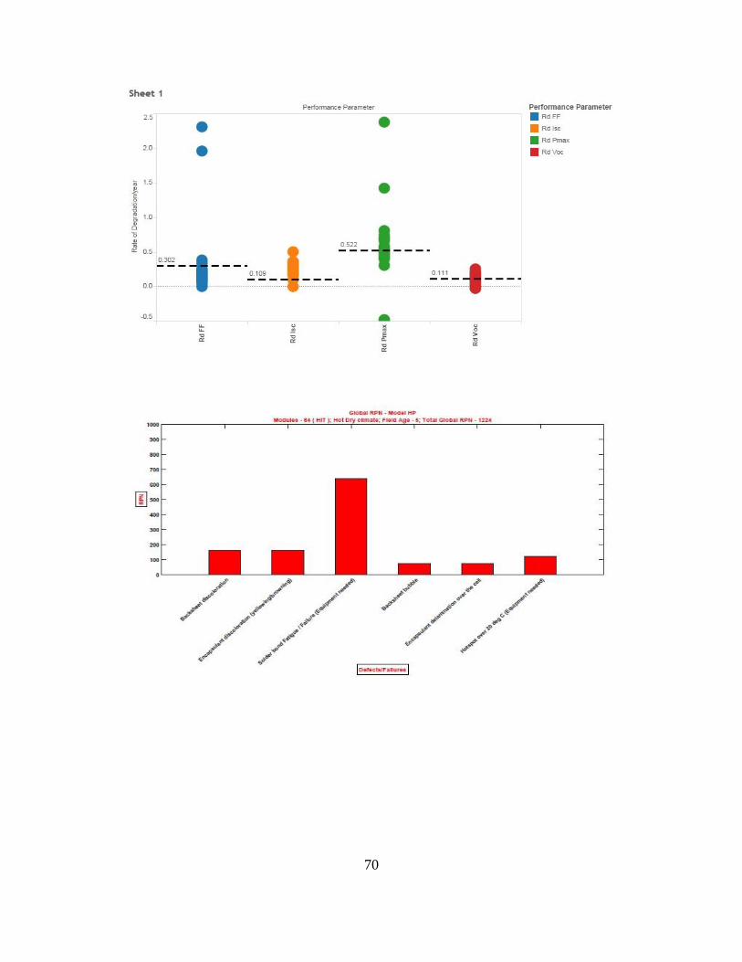
70

71

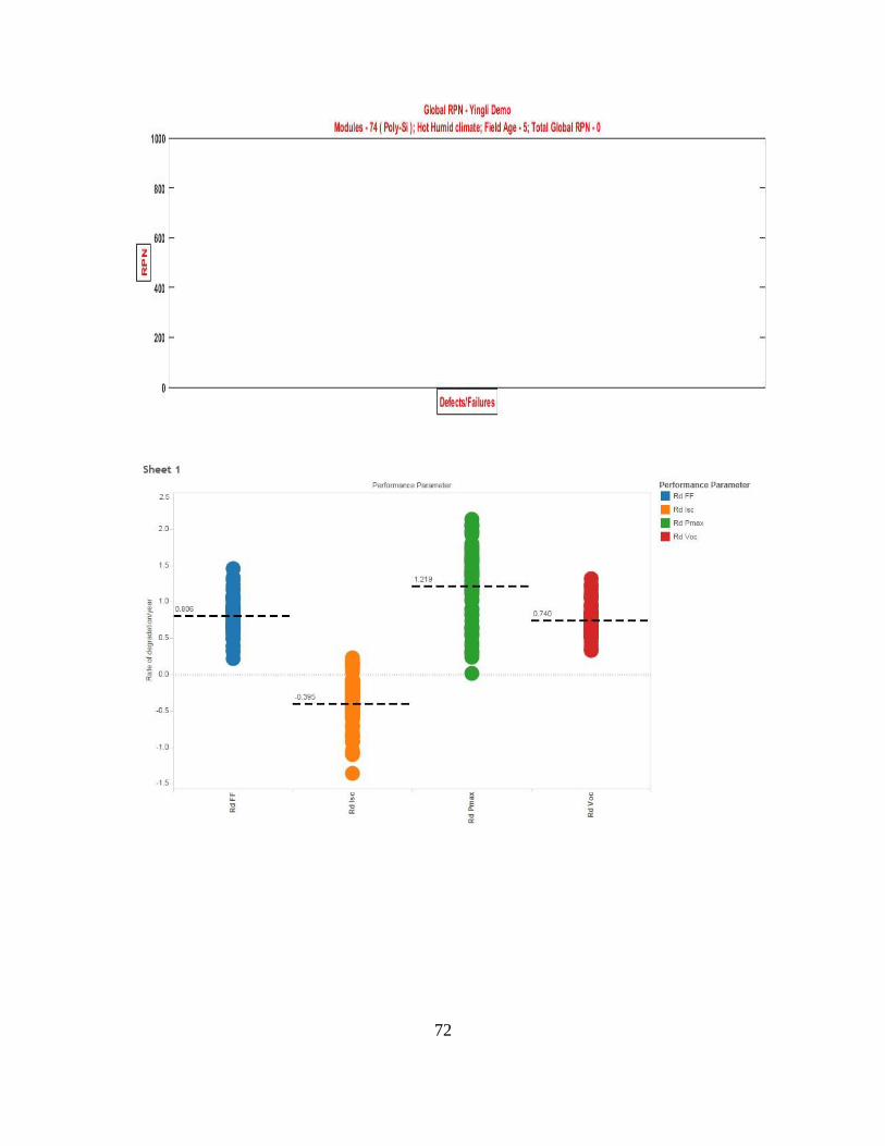
72

73

74

75

76