Federal Reserve Bank of Dallas Globalization and Monetary Policy Institute

Working Paper No. 19 http://www.dallasfed.org/assets/documents/institute/wpapers/2008/0019.pdf

Default and the Maturity Structure in Sovereign Bonds*

Cristina Arellano

University of Minnesota Federal Reserve Bank of Minneapolis

Ananth Ramanarayanan

Federal Reserve Bank of Dallas

August 2008 Revised: April 2010

Abstract During emerging market crises, government interest rate spreads rise, the debt maturity shortens and the spread on short-term bonds is higher than on long-term bonds. This paper studies the maturity composition of debt in a dynamic model with endogenous default, in which the price of debt compensates for the risk-adjusted losses from default. Short-term debt is better at inducing repayment because it does not require savings in the near future for repaying in the far future. Hence, short-term debt can raise more resources than long-term debt. However, issuing long-term debt provides a hedge against the need to roll-over short-term debt at high interest rate spreads. The trade-off between these two benefits is quantitatively important for understanding the maturity composition in emerging markets. When calibrated to data from Brazil, the model matches the dynamics in the maturity of debt issuances and its comovement with the level of spreads across maturities. JEL codes: F34, G15

* Cristina Arellano, Department of Economics, University of Minnesota, 4-101 Hanson Hall, 1925 Fourth Street South, Minneapolis, MN 55455. arellano@econ.umn.edu. Ananth Ramanarayanan, Research Department, Federal Reserve Bank of Dallas, 2200 North Pearl Street, Dallas, TX 75201 ananth.ramanarayanan@gmail.com. We thank V. V. Chari, Hugo Hopenhayn, Tim Kehoe, Patrick Kehoe, Narayana Kocherlakota, Hanno Lustig, Enrique Mendoza, Fabrizio Perri, Victor Rios-Rull, and Diego Valderrama for many useful comments. The views in this paper are those of the authors and do not necessarily reflect the views of the Federal Reserve Bank of Dallas or the Federal Reserve System.

1 Introduction

Debt crises in emerging economies are often blamed on governments borrowing large amounts

of short-term debt in international capital markets. Short-term borrowing leaves an economy

with large amounts of debt to roll over, which becomes difficult when interest rates rise and

access to external credit is restricted. This idea has motivated several recent empirical studies

on debt and financial crises. For example, Rodrik and Velasco (2003) show, using evidence

from a broad set of countries, that a high level of short-term foreign debt increases the

likelihood of a crisis.1 From this ex post point of view, it seems desirable to implement

policies that would lengthen the maturity structure of emerging market economies’ external

liabilities. However, as documented by Broner, Lorenzoni, and Schmukler (2008), emerging

market governments actively shift to shorter-maturity debt in a crisis and issue long-term

debt in normal times. While this pattern may leave countries more exposed to roll-over crises

in bad times, it suggests that there must be some benefits, ex ante, of shortening the maturity

structure of debt precisely in such times. By the same token, the benefits of long-term debt

must outweigh those of short-term debt in normal times.

In this paper, we develop a model of sovereign debt in which the borrower endogenously

chooses a time-varying maturity structure of debt. The model accounts for the following

observation in the data: when interest rate spreads rise, the short-term spread rises more

than the long-term spread, while the maturity of newly issued debt shortens. Bond prices

reflect the risk adjusted loss in case of default and are jointly determined along with the

maturity structure of debt. Hence, we examine the maturity choice in a framework with

realistic predictions for the term structure of interest rate spreads. Our model can rationalize

shorter debt maturity during crises as the result of a liquidity advantage in short-term debt

contracts; although these contracts carry higher spreads than longer term debt, they can

deliver more resources to the country in times of high default risk.

We present data on prices and issuances of foreign-currency denominated bonds for four

emerging market countries: Argentina, Brazil, Mexico, and Russia. We estimate spread

curves — interest rate spreads over U.S. Treasury bonds across maturity — as well as the

duration of bonds issued — a measure of the average time to maturity of payments on coupon-

paying bonds. Across these four countries, within periods in which 2-year spreads are below

their 25th percentile, the average duration of new debt is 7.1 years, and the average difference

1Other detailed studies on individual cases include Calvo and Mendoza (1996) for Mexico; Radelet andSachs (1998) for the East Asian economies; and Bevilaqua and Garcia (2002) for Brazil. Cole and Kehoe(1996) use a model of self-fulfilling crises to argue that the 1994 Mexican debt crisis could have been avoidedif the maturity of government debt had been longer.

2

between the 10-year spread and the 2-year spread — the slope of the spread curve — is 2.3

percentage points. But when the 2-year spreads are above their 75th percentile, the average

duration shortens to 5.7 years, while the slope of the spread curve is −0.5 percentage points.From this evidence we conclude that the maturity of debt shortens in times of high spreads

and downward-sloping spread curves.

In our model, a borrower faces persistent income shocks and can issue long and short

duration bonds. The borrower can default on debt at any point in time, but faces costs of

doing so, in the form of lower income and exclusion from international financial markets. In

equilibrium, default tends to occur in low-income, high-debt times, when the cost of debt

payments outweighs the costs of default. Bond prices compensate for the expected loss from

default as well as for risk premia.

Our model generates the dynamics of spread curves observed in the data because the

endogenous probability of repayment is persistent, yet mean reverting, as a result of the

dynamics of debt and income. In times of low debt and high income, default is unlikely in

the near future, so spreads are low. Long-term spreads are higher than short-term spreads

because default may become likely in the far future if the borrower receives a sequence of

bad shocks and accumulates debt. Long-term spreads are also higher because of the risk

premium on future changes in default probabilities. Conversely, in times of low income and

high debt, default is likely in the near future, so spreads are high. Long-term spreads rise

less than short-term spreads because the borrower’s likelihood of repaying may rise over a

longer time horizon if a sequence of good shocks occurs and debt is reduced.

We calibrate the model to Brazil and find that it fits the observed dynamics of spreads

well. When the spread on 2-year debt is below its 25th percentile, the 10-year spread is

on average 2 percentage points higher than the 2-year spread, compared to a slope of 3

percentage points in Brazil. In periods when the 2-year spread is above its 75th percentile,

the slope of the spread curve in the model inverts to−0.9 percentage points, compared to−1.5percentage points in Brazil. We also use the model to decompose spreads into actuarially fair

compensation for default and risk premia. We find that risk premia account for a substantial

portion of the spread in periods of low spreads, but that the majority of the changes in

spreads are accounted for by the dynamics of the default probability. For example, the risk

premium accounts on for one third of the 2-year spread when 2-year spreads are below their

25th percentile, but only for five percent when 2-year spreads are above their 75th percentile.

In addition, the risk premium on long-term debt is always higher than on short-term debt,

reflecting the fact that the risk premium is cumulated over a longer horizon. This allows the

model to generate an average slope of the spread curve of about 1 percentage point, compared

3

to 1.5 percentage points in the Brazilian data.

The maturity structure of debt in the model reflects a trade-off between liquidity benefits

of short-term debt and hedging benefits of long-term debt, both due to the presence of default.

Short-term debt is a more liquid asset in the sense that consumption can be increased more

effectively with short-term debt than with long-term debt. Issuing short-term debt induces

the borrower to repay income in the near future to avoid the costs of defaulting. In contrast,

the borrower cannot commit to saving sufficiently to repay long-term debt, so consumption

cannot be raised as much with long-term debt.

Despite its liquidity benefits, short-term debt is risky, in the sense that rolling over a

lot of short-term debt is expensive in future states with high interest rate spreads. Issuing

long-term debt provides a hedge, because its value falls in bad states more than the value

of short-term debt. This lowers the total debt burden in bad states relative to good states,

effectively transferring resources across states in future periods. The value of outstanding

long-term debt reflects cumulative risk-adjusted default probabilities over a longer horizon,

so it is more sensitive to changes in default risk than the value of short-term debt.

The time-varying maturity structure in the model is a result of the time-varying valuation

of the liquidity benefit of short-term debt and the hedging benefit of long-term debt. Periods

of low default probabilities and upward-sloping spread curves correspond to states when the

borrower is wealthy and values the hedging benefit that long-term debt provides. Thus, the

portfolio is shifted toward long debt. Periods of high default probabilities and inverted spread

curves correspond to states when the borrower is poor and credit is limited. These are times

when liquidity is most valuable, and thus the portfolio is shifted toward shorter-term debt.

In these periods, the average duration of debt is about 2.4 years shorter than in periods

with low spreads, compared to a difference of about 1.7 years in Brazil. We can therefore

rationalize higher short-term debt positions in times of crises as an optimal response to the

illiquidity of long-term debt, and the tighter availability of its supply.

Risk premia in bond prices have substantial effects on default probabilities and the ma-

turity of debt. In a counterfactual exercise, we find that raising risk premia makes borrowing

more costly, which results in lower default probabilities in equilibrium. High risk premia

also shorten the maturity of debt because they disproportionately raise the cost of issuing

long-term debt.

Related Literature

Several recent papers study the maturity structure of sovereign debt. Jeanne (2009) argues

that short-term debt gives incentives for sovereign governments to implement creditor-friendly

4

policies, because creditors can discipline the government by rolling over the debt only after

desired policies are implemented. In our model, short-term debt also plays a role in inducing

the government to repay when it lacks the ability to commit to repayment. Relative to

Jeanne (2009), we consider why debt maturity shortens in times of high spreads. Broner,

Lorenzoni, and Schmukler (2008) argue that emerging markets shift to short-term debt in

a crisis because shocks to lenders’ risk aversion raise the risk premium on long-term bonds

more than on short-term bonds. In our model, we allow for time-varying risk premia, but

the lenders’ degree of risk aversion fluctuates with the borrower’s income, instead of being

driven by independent shocks.2

The mechanisms in our model build on two strands of the corporate finance literature.

First, the basic tradeoff between issuing short-term and long-term debt in our model is

similar to that discussed by Hart and Moore (1989, 1994). They develop a model in which

an entrepreneur who cannot commit to repay seeks financing for a project from a lender.3

In addition, our results on the term structure of spreads mirror those derived in Merton

(1974) for credit spread curves on defaultable corporate bonds. Our framework differs from

Merton’s in that the probability of default and the level and maturity composition of debt

issuances are endogenous.

This paper is also related to the literature on the optimal maturity structure of government

debt in closed economies. Angeletos (2002), Buera and Nicolini (2004) and Shin (2007) show

that, when debt is not state contingent, a rich maturity structure of government bonds

can be used to replicate the allocations obtained with state-contingent debt in economies

with distortionary taxes as in Lucas and Stokey (1983). In these models, short- and long-

term interest rate dynamics reflect the variation in the representative agent’s marginal rate

of substitution, which changes with the state of the economy. Lustig, Sleet, and Yeltekin

(2006) show that higher interest rates on long-term debt relative to short-term debt reflect

an insurance premium paid by the government for the benefits long-term debt provides

in hedging against future shocks. Our paper shares with these papers the message that

managing the maturity composition of debt can provide benefits to the government because

of fluctuations in future interest rates.4

The model in this paper builds on the work of Aguiar and Gopinath (2006) and Arellano

2Bi (2007) and Niepelt (2009) present dynamic models focusing on other mechanisms. Bi shows how short-term debt reduces the value of outstanding long-term debt, while Niepelt focuses on smoothing borrowingcosts across maturities.

3Diamond (1991) emphasizes a similar tradeoff in a model in which borrowers have private informationover their future default risk.

4Neumeyer and Perri (2005) have shown that emerging markets face substantial fluctuations in interestrate spreads, which makes hedging interest rate fluctuations particularly useful.

5

(2008), who model equilibrium default with incomplete markets, as in the seminal paper

on sovereign debt by Eaton and Gersovitz (1981). To connect our model to the data, we

extend this framework to incorporate long debt of multiple maturities, rather than one-

period debt as in these earlier papers, as well as a flexible pricing kernel that allows for risk

premia in bond prices. In recent work, Chatterjee and Eyigungor (2009) and Hatchondo and

Martinez (2009) show that models with a single long-term defaultable bond allow a better fit

of emerging market data in terms of the volatility and mean of the country spread as well as

debt levels. In addition, Borri and Verdelhan (2009) show that risk premia help to explain

the variation of spreads across emerging markets with similar default probabilities.

The outline of the paper is as follows. Section 2 presents data on the dynamics of the

spread curve and maturity composition for four emerging markets: Argentina, Brazil, Mexico,

and Russia. Section 3 presents the theoretical model. Section 4 presents some examples to

illustrate the mechanisms that determine the optimal debt portfolio. Section 5 presents all

the quantitative results, and Section 6 concludes.

2 Emerging Markets Bond Data

We examine data on sovereign bonds issued in international financial markets by four emerging-

market countries: Argentina, Brazil, Mexico, and Russia. We look at the behavior of the

interest rate spreads over default-free bonds, across different maturities, and at the way the

maturity of new debt issued covaries with spreads. We find that when spreads are low, govern-

ments issue long-term bonds more heavily and long-term spreads are higher than short-term

spreads. When spreads rise, the maturity of bond issuances shortens and short-term spreads

are higher than long-term spreads. Our findings confirm the earlier results of Broner, Loren-

zoni, and Schmukler (2008), who showed in a sample of eight emerging economies that debt

maturity shortens when spreads are very high.5

2.1 Spread Curves

We define the n-year spread for an emerging market country as the difference between the

yield on a defaultable, zero-coupon bond maturing in n years issued by the country and on

a zero-coupon bond of the same maturity with negligible default risk (for example, a U.S.

5Broner, Lorenzoni and Schmukler (2008) focus on the relationship between the term structure of excessreturns and the average maturity of debt. In this section we construct measures of the term structure ofyield spreads and the average duration of debt because these statistics provide the basis for the quantitativeassessment of our model.

6

Treasury note). The spread is the implicit interest rate premium required by investors to be

willing to purchase a defaultable bond of a given maturity. The spread curve depicts spreads

as a function of maturity.

We denote the continuously compounded yield at date t on a zero-coupon bond issued

by country i, maturing in n years, as rnt,i. The yield is related to the price pnt,i of an n-year

zero-coupon bond, with face value 1, through

pnt,i = exp(−n× rnt,i). (1)

The n-year spread for country i at date t is given by: snt,i = rnt,i − rnt,rf , where rnt,rf is the

yield of a n-year default-free bond.6

Since governments do not issue zero-coupon bonds in a wide range of maturities, we

estimate a country’s spread curve by using secondary market data on the prices at which

coupon-bearing bonds trade. The estimation procedure consists of choosing a functional

form for the spread curve to fit the discounted value of coupon payments to prices, following

Svensson (1994) and Broner, Lorenzoni, and Schmukler (2008). We describe this procedure

further in the Appendix and illustrate that the resulting pricing errors are small.

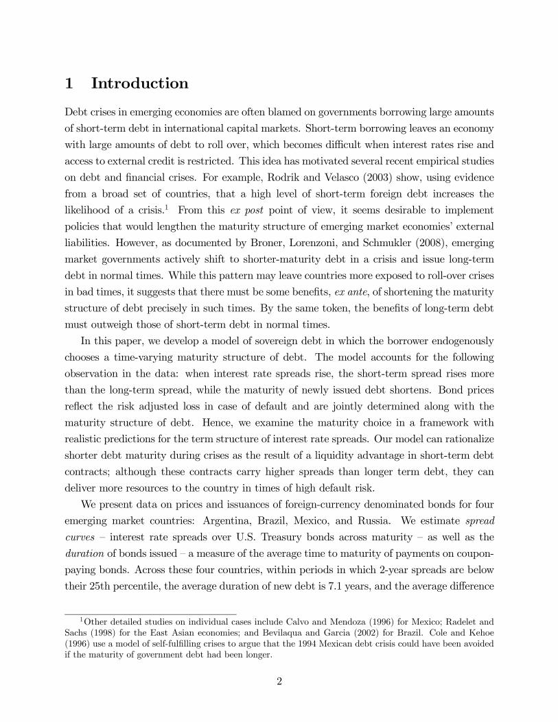
We compute spreads starting in March 1996 at the earliest and ending in May 2004 at the

latest, depending on the availability of data for each country. Figure 1 displays the estimated

spreads for 2-year and 10-year bonds for Argentina, Brazil, Mexico, and Russia.

Spreads are very volatile, and the difference between long-term and short-term spreads

varies substantially over time. When spreads are low, long-term spreads are generally higher

than short-term spreads. However, when the level of spreads rises, the gap between long

and short-term spreads tends to narrow and sometimes reverses: the spread curve flattens or

inverts. The time series in Figure 1 show sharp increases in interest rate spreads associated

with Russia’s default in 1998, Argentina’s default in 2001, and Brazil’s financial crisis in

2002.7 The expectation that the countries would default in these episodes is reflected in the

high spreads charged on defaultable bonds.

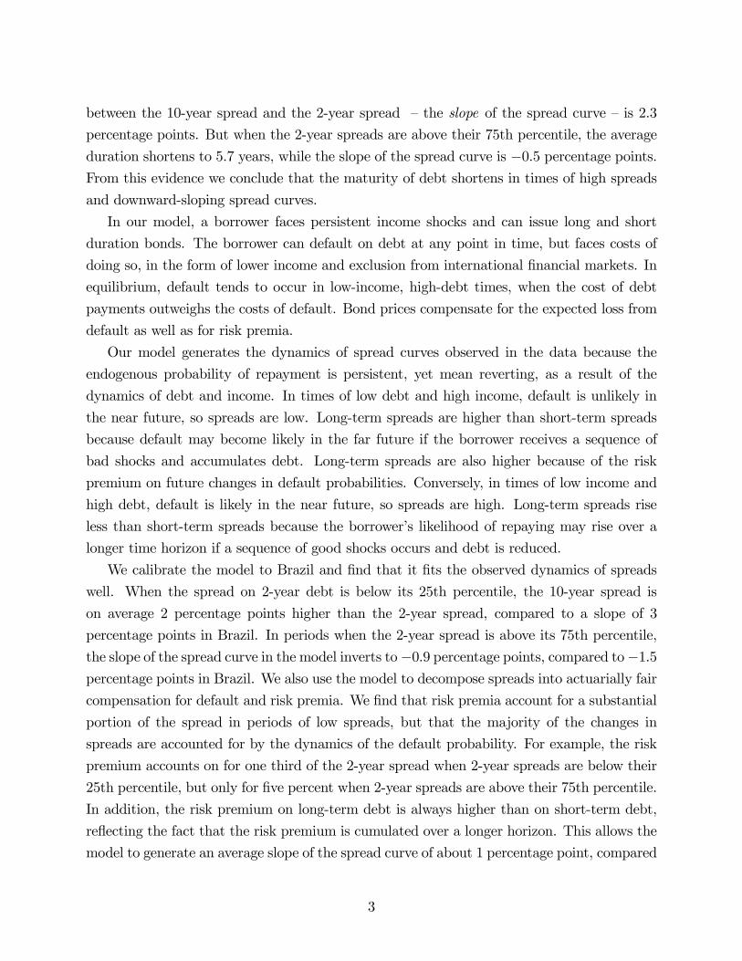
To emphasize the pattern observed in the time series that short-term spreads tend to rise

more than long-term spreads, in Figure 2 we display spread curves averaged across different

6Our data include bonds denominated in U.S. dollars and European currencies, so we take U.S. andEuro-area government bond yields as default-free.

7For Argentina and Russia, we do not report spreads after default on external debt, unless a restructuringagreement was largely completed at a later date. We use dates taken from Sturzenegger and Zettelmeyer(2005). For Argentina, we report spreads until the last week of December 2001, when the country defaulted.The restructuring agreement for external debt was not offered until 2005. For Russia, we report spreads untilthe second week of August 1998 and beginning again after August 2000 when 75% of external debt had beenrestructured.

7

96 97 98 99 00 01 02 03 040

5

10

15

20

25

30

date

spre

ad (

%)

Argentina

96 97 98 99 00 01 02 03 040

5

10

15

20

25

30

date

spre

ad (

%)

Brazil

96 97 98 99 00 01 02 03 040

5

10

15

20

25

30

date

spre

ad (

%)

Mexico

96 97 98 99 00 01 02 03 040

5

10

15

20

25

30

date

spre

ad (

%)

Russia

2 year

10 year

Figure 1: Time Series of Short and Long Spreads

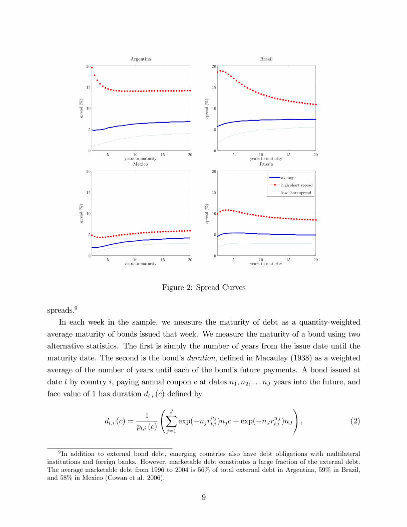
time periods for each country: the overall average, the average within periods with the 2-year

spread below its 10th percentile, and the average within periods with the 2-year spread above

its 90th percentile. When spreads are low, the spread curve is upward sloping: long-term

spreads are higher than short-term spreads. When spreads are high, short-term spreads rise

more than long-term spreads. For Argentina, Brazil, and Russia, the spread curve becomes

downward sloping in these times. For Mexico, which had relatively smaller increases in

spreads during this time period, the spread curve flattens as short spreads rise more than

long spreads.8

2.2 The Maturity Composition of Debt and Spreads

We now examine the maturity of new debt issued by the four emerging market economies

during the sample period, and relate the changes in the maturity of debt to changes in

8The findings are similar to empirical findings on spread curves in corporate debt markets. Sarig andWarga (1989), for example, find that highly rated corporate bonds have low levels of spreads, and spreadcurves that are flat or upward-sloping, while low-grade corporate bonds have high levels of spreads, andaverage spread curves that are hump-shaped or downward-sloping.

8

5 10 15 200

5

10

15

20

Argentina

years to maturity

spre

ad (

%)

5 10 15 200

5

10

15

20

Brazil

years to maturity

spre

ad (

%)

5 10 15 200

5

10

15

20

Mexico

years to maturity

spre

ad (

%)

5 10 15 200

5

10

15

20

years to maturity

spre

ad (

%)

Russia

average

high short spread

low short spread

Figure 2: Spread Curves

spreads.9

In each week in the sample, we measure the maturity of debt as a quantity-weighted

average maturity of bonds issued that week. We measure the maturity of a bond using two

alternative statistics. The first is simply the number of years from the issue date until the

maturity date. The second is the bond’s duration, defined in Macaulay (1938) as a weighted

average of the number of years until each of the bond’s future payments. A bond issued at

date t by country i, paying annual coupon c at dates n1, n2, . . . nJ years into the future, and

face value of 1 has duration dt,i (c) defined by

dt,i (c) =1

pt,i (c)

ÃJXj=1

exp(−njrnjt,i )njc+ exp(−nJrnJt,i )nJ

!, (2)

9In addition to external bond debt, emerging countries also have debt obligations with multilateralinstitutions and foreign banks. However, marketable debt constitutes a large fraction of the external debt.The average marketable debt from 1996 to 2004 is 56% of total external debt in Argentina, 59% in Brazil,and 58% in Mexico (Cowan et al. 2006).

9

where pt,i (c) is the coupon bond’s price, and rnt,i is the zero-coupon yield curve. The time

until each future payment is weighted by the discounted value of that payment relative to

the price of the bond. A zero-coupon bond has duration equal to the number of years until

its maturity date, but a coupon-paying bond has duration shorter than its time to maturity.

We consider duration as a measure of maturity because it is more comparable across bonds

with different coupon rates.

We calculate the average maturity and average duration of new bonds issued in each

week by each country. Table 1 displays each country’s averages of these weekly maturity

and duration series within periods of high (above median) and low (below median) 2-year

spreads.

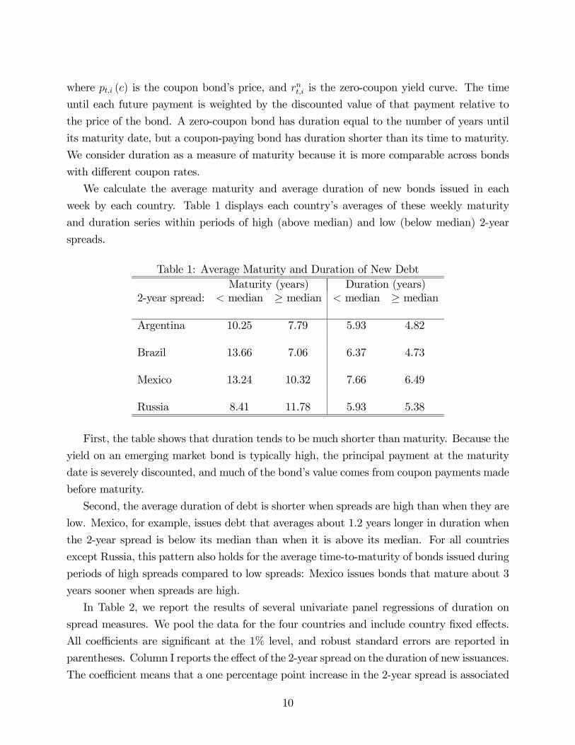
Table 1: Average Maturity and Duration of New DebtMaturity (years) Duration (years)

2-year spread: < median ≥ median < median ≥ median

Argentina 10.25 7.79 5.93 4.82

Brazil 13.66 7.06 6.37 4.73

Mexico 13.24 10.32 7.66 6.49

Russia 8.41 11.78 5.93 5.38

First, the table shows that duration tends to be much shorter than maturity. Because the

yield on an emerging market bond is typically high, the principal payment at the maturity

date is severely discounted, and much of the bond’s value comes from coupon payments made

before maturity.

Second, the average duration of debt is shorter when spreads are high than when they are

low. Mexico, for example, issues debt that averages about 1.2 years longer in duration when

the 2-year spread is below its median than when it is above its median. For all countries

except Russia, this pattern also holds for the average time-to-maturity of bonds issued during

periods of high spreads compared to low spreads: Mexico issues bonds that mature about 3

years sooner when spreads are high.

In Table 2, we report the results of several univariate panel regressions of duration on

spread measures. We pool the data for the four countries and include country fixed effects.

All coefficients are significant at the 1% level, and robust standard errors are reported in

parentheses. Column I reports the effect of the 2-year spread on the duration of new issuances.

The coefficient means that a one percentage point increase in the 2-year spread is associated

10

with a decrease in the duration of new debt issued by just under half a year. Column 2 shows

a similar effect for the 10-year spread. These figures indicate that the covariation between

the duration of new debt issuance and interest rate spreads is both economically large and

statistically significant.10

Table 2: Regressions of Duration of New Issuances on SpreadsI II III

Variable

2-year spread−0.446∗∗∗(0.116)

10-year spread−0.394∗∗∗(0.102)

10/2 ratio0.543∗∗∗

(0.162)R2 0.201 0.195 0.157No. of obs. 151 151 151

Note: All specifications include a constant. Robust standard errors are

reported in parentheses, and ∗∗∗ denotes significance at the 1% level.

In Table 3, we emphasize the relationship between the spread curve slopes and average

duration. The slope of the spread curve, defined here as the difference between the 10-year

(long-term) and 2-year (short-term) spread, falls when the 2-year spread is high — the numbers

in column 4 of Table 3 are smaller than those in column 3. During these times, however,

the countries shift toward short-term debt, even though the spreads on long-term debt rise

less than for short-term debt. In Brazil, for example, while the spread curve changes from

depicting a 10-year spread that is about 3 percentage points above the 2-year spread to one

that is 1.41 percentage points below the 2-year spread, the average duration of newly issued

debt reduces by more than 2 years.

Column III of Table 2 shows that the duration of new debt is positively associated with

how large the 10-year spread is relative to the 2-year spread. When the ratio of the long

spread to the short spread increases by one, the duration of new debt rises by about half a

year.

10These estimates mirror the findings in Broner, Lorenzoni, and Schmukler (2008). They show that ahigh spread level is a statistically significant determinant for a shorter maturity of debt issuances even aftercontrolling for selection effects due the fact that the timing of debt issuances is very irregular. Their empiricalwork treats the issuance of short-term or long-term debt as a discrete variable, whereas we use the continuousvariable of duration as a measurement of maturity.

11

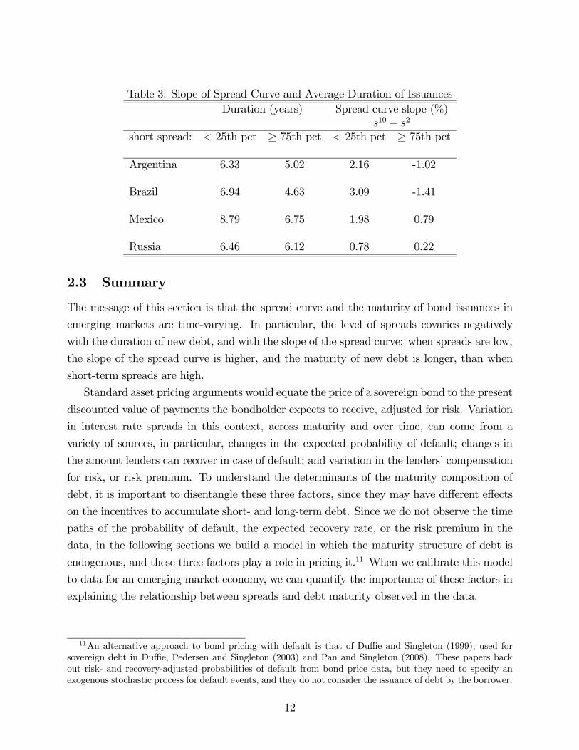
Table 3: Slope of Spread Curve and Average Duration of IssuancesDuration (years) Spread curve slope (%)

s10 − s2

short spread: < 25th pct ≥ 75th pct < 25th pct ≥ 75th pct

Argentina 6.33 5.02 2.16 -1.02

Brazil 6.94 4.63 3.09 -1.41

Mexico 8.79 6.75 1.98 0.79

Russia 6.46 6.12 0.78 0.22

2.3 Summary

The message of this section is that the spread curve and the maturity of bond issuances in

emerging markets are time-varying. In particular, the level of spreads covaries negatively

with the duration of new debt, and with the slope of the spread curve: when spreads are low,

the slope of the spread curve is higher, and the maturity of new debt is longer, than when

short-term spreads are high.

Standard asset pricing arguments would equate the price of a sovereign bond to the present

discounted value of payments the bondholder expects to receive, adjusted for risk. Variation

in interest rate spreads in this context, across maturity and over time, can come from a

variety of sources, in particular, changes in the expected probability of default; changes in

the amount lenders can recover in case of default; and variation in the lenders’ compensation

for risk, or risk premium. To understand the determinants of the maturity composition of

debt, it is important to disentangle these three factors, since they may have different effects

on the incentives to accumulate short- and long-term debt. Since we do not observe the time

paths of the probability of default, the expected recovery rate, or the risk premium in the

data, in the following sections we build a model in which the maturity structure of debt is

endogenous, and these three factors play a role in pricing it.11 When we calibrate this model

to data for an emerging market economy, we can quantify the importance of these factors in

explaining the relationship between spreads and debt maturity observed in the data.

11An alternative approach to bond pricing with default is that of Duffie and Singleton (1999), used forsovereign debt in Duffie, Pedersen and Singleton (2003) and Pan and Singleton (2008). These papers backout risk- and recovery-adjusted probabilities of default from bond price data, but they need to specify anexogenous stochastic process for default events, and they do not consider the issuance of debt by the borrower.

12

3 The Model

We consider a dynamic model of defaultable debt that includes bonds of short and long

duration. A small open economy receives a stochastic stream of income, y that follows a

Markov process with compact support and transition function f(yt, yt+1). The economy

trades two bonds of different duration with international lenders. Financial contracts are

unenforceable, so the economy can default on its debt at any time. If the economy defaults,

it temporarily loses access to international financial markets and also incurs direct costs.

The representative agent in the small open economy (henceforth, the “borrower”) receives

utility from consumption ct and has preferences given by

E∞Xt=0

βtu(ct), (3)

where 0 < β < 1 is the time discount factor and u(·) is increasing and concave.The borrower issues debt in the form of two types of perpetuity contracts with coupon

payments that decay geometrically. We let {δS, δL} ∈ [0, 1] denote the “decay factors” of thepayments for the two bonds. A perpetuity with decay factor δm is a contract that specifies

a price qmt and a loan face value mt such that the borrower receives q

mt

mt units of goods in

period t and promises to pay, conditional on not defaulting, δn−1mmt units of goods in every

future period t + n. The decay of each perpetuity is related to its duration: a bond of

this type with rapidly declining payments has a larger proportion of its value paid early on,

and therefore a shorter duration, than a bond with more slowly declining payments. We let

δS < δL, so that δS is the decay of the perpetuity with short duration and δL is the decay of

the perpetuity with long duration. We will refer to the perpetuities with decay factors δS and

δL throughout as short and long bonds, respectively. Each one of our bonds resembles the

long-duration bond in Hatchondo and Martinez (2009) and Rudebusch and Swanson (2008).

By having two such assets, we allow the borrower to choose the maturity composition of debt

each period.

At every date t the economy has outstanding all past bond issuances. Define bmt , the

stock of bonds of duration m at time t, as the total payments due in period t on all past

issuances of type m, conditional on not defaulting:

bmt =tX

j=1

δj−1mmt−j =

mt−1 + δm

mt−2 + δ2m

mt−3 + ...+ δtm

m0 + bm0 ,

where bm0 is given. Thus, the accumulation for the stocks of short and long perpetuities can

13

be written recursively by the following laws of motion:

bSt+1 = δSbSt +

St (4)

bLt+1 = δLbLt +

Lt

With these definitions, we can compactly write the borrower’s budget constraint condi-

tional on not defaulting. Purchases of consumption are constrained by the endowment less

payments on outstanding debt, bSt + bLt , plus the issues of new short bondsSt at price q

St and

long bonds Lt at a price q

Lt :

ct = yt − bSt − bLt + qStSt + qLt

Lt (5)

The borrower chooses new issues of perpetuities from a menu of contracts where prices qStand qLt for are quoted for each pair (b

St+1, b

Lt+1).

If the borrower defaults, we assume that all outstanding debts and assets (bSt + bLt ) are

erased from the budget constraint, and the economy cannot borrow or save, so that con-

sumption equals output. In addition, the country incurs output costs:

ydeft =

(yt if yt ≤ (1− λ)y

(1− λ)y if yt > (1− λ)y,

where y is the mean level of output. This specification, following Arellano (2008), assumes

that borrowers lose a fraction λ of output if output is above a threshold.

3.1 Recursive Problem

We represent the borrower’s infinite horizon decision problem as a recursive dynamic pro-

gramming problem. The model has two endogenous states — the stocks of each type of debt,

bSt and bLt — and one exogenous state, the income of the economy, yt. The state of the economy

at date t is then given by (bS, bL, y) ≡ (bSt , bLt , yt).At any given state, the value of the option to default is given by

vo(bS, bL, y) = maxc,d

©vc(bS, bL, y), v

d(y)ª, (6)

where vc(bS, bL, y) is the value associated with not defaulting and staying in the contract and

vd(y) is the value associated with default.

Since we assume that default costs are incurred whenever the borrower fails to repay its

14

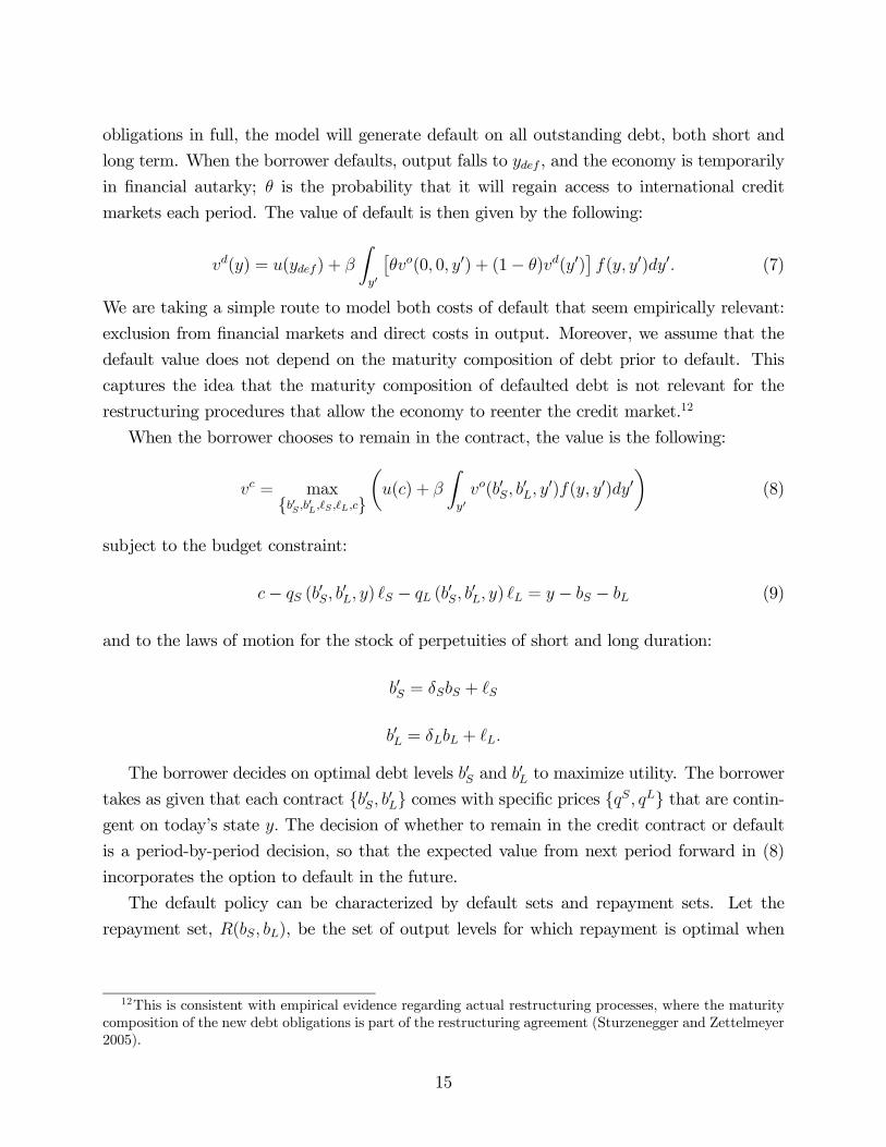
obligations in full, the model will generate default on all outstanding debt, both short and

long term. When the borrower defaults, output falls to ydef , and the economy is temporarily

in financial autarky; θ is the probability that it will regain access to international credit

markets each period. The value of default is then given by the following:

vd(y) = u(ydef) + β

Zy0

£θvo(0, 0, y0) + (1− θ)vd(y0)

¤f(y, y0)dy0. (7)

We are taking a simple route to model both costs of default that seem empirically relevant:

exclusion from financial markets and direct costs in output. Moreover, we assume that the

default value does not depend on the maturity composition of debt prior to default. This

captures the idea that the maturity composition of defaulted debt is not relevant for the

restructuring procedures that allow the economy to reenter the credit market.12

When the borrower chooses to remain in the contract, the value is the following:

vc = max{b0S ,b0L, S , L,c}

µu(c) + β

Zy0vo(b0S, b

0L, y

0)f(y, y0)dy0¶

(8)

subject to the budget constraint:

c− qS (b0S, b

0L, y) S − qL (b

0S, b

0L, y) L = y − bS − bL (9)

and to the laws of motion for the stock of perpetuities of short and long duration:

b0S = δSbS + S

b0L = δLbL + L.

The borrower decides on optimal debt levels b0S and b0L to maximize utility. The borrower

takes as given that each contract {b0S, b0L} comes with specific prices {qS, qL} that are contin-gent on today’s state y. The decision of whether to remain in the credit contract or default

is a period-by-period decision, so that the expected value from next period forward in (8)

incorporates the option to default in the future.

The default policy can be characterized by default sets and repayment sets. Let the

repayment set, R(bS, bL), be the set of output levels for which repayment is optimal when

12This is consistent with empirical evidence regarding actual restructuring processes, where the maturitycomposition of the new debt obligations is part of the restructuring agreement (Sturzenegger and Zettelmeyer2005).

15

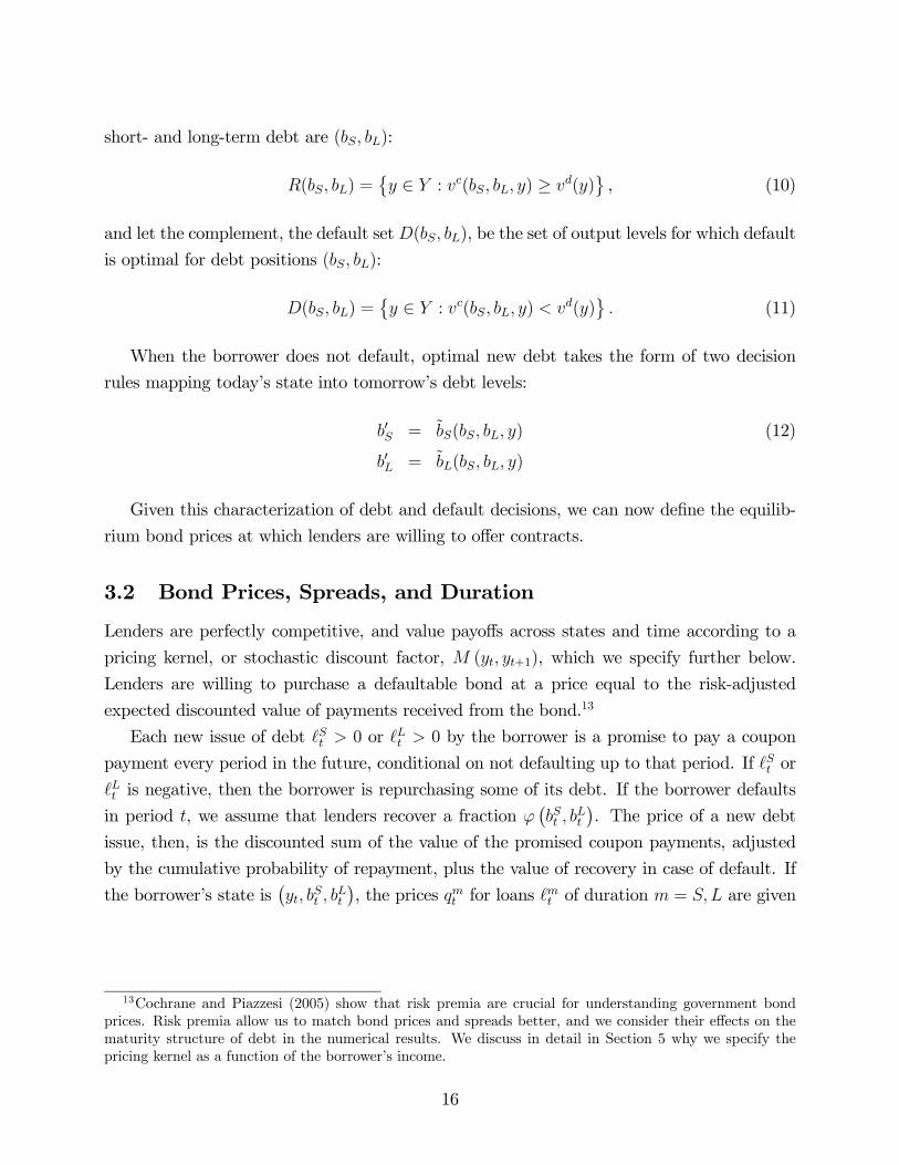
short- and long-term debt are (bS, bL):

R(bS, bL) =©y ∈ Y : vc(bS, bL, y) ≥ vd(y)

ª, (10)

and let the complement, the default set D(bS, bL), be the set of output levels for which default

is optimal for debt positions (bS, bL):

D(bS, bL) =©y ∈ Y : vc(bS, bL, y) < vd(y)

ª. (11)

When the borrower does not default, optimal new debt takes the form of two decision

rules mapping today’s state into tomorrow’s debt levels:

b0S = bS(bS, bL, y) (12)

b0L = bL(bS, bL, y)

Given this characterization of debt and default decisions, we can now define the equilib-

rium bond prices at which lenders are willing to offer contracts.

3.2 Bond Prices, Spreads, and Duration

Lenders are perfectly competitive, and value payoffs across states and time according to a

pricing kernel, or stochastic discount factor, M (yt, yt+1), which we specify further below.

Lenders are willing to purchase a defaultable bond at a price equal to the risk-adjusted

expected discounted value of payments received from the bond.13

Each new issue of debt St > 0 or L

t > 0 by the borrower is a promise to pay a coupon

payment every period in the future, conditional on not defaulting up to that period. If St or

Lt is negative, then the borrower is repurchasing some of its debt. If the borrower defaults

in period t, we assume that lenders recover a fraction ϕ¡bSt , b

Lt

¢. The price of a new debt

issue, then, is the discounted sum of the value of the promised coupon payments, adjusted

by the cumulative probability of repayment, plus the value of recovery in case of default. If

the borrower’s state is¡yt, b

St , b

Lt

¢, the prices qmt for loans

mt of duration m = S,L are given

13Cochrane and Piazzesi (2005) show that risk premia are crucial for understanding government bondprices. Risk premia allow us to match bond prices and spreads better, and we consider their effects on thematurity structure of debt in the numerical results. We discuss in detail in Section 5 why we specify thepricing kernel as a function of the borrower’s income.

16

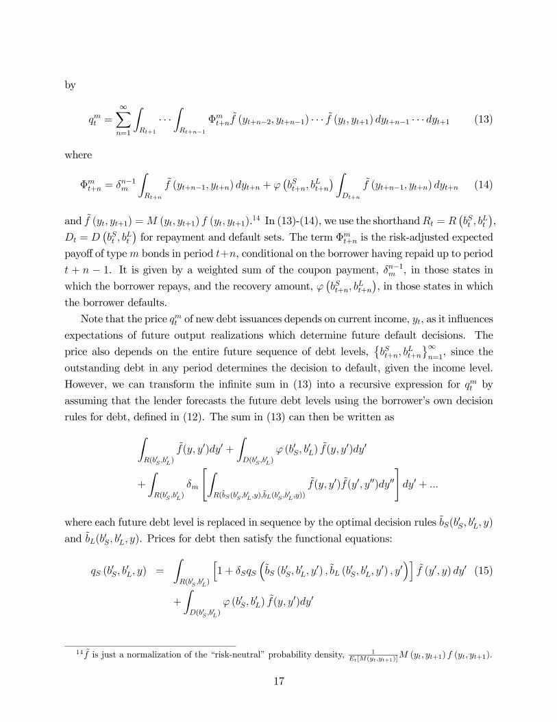
by

qmt =∞Xn=1

ZRt+1

· · ·ZRt+n−1

Φmt+nf (yt+n−2, yt+n−1) · · · f (yt, yt+1) dyt+n−1 · · · dyt+1 (13)

where

Φmt+n = δn−1m

ZRt+n

f (yt+n−1, yt+n) dyt+n + ϕ¡bSt+n, b

Lt+n

¢ ZDt+n

f (yt+n−1, yt+n) dyt+n (14)

and f (yt, yt+1) =M (yt, yt+1) f (yt, yt+1).14 In (13)-(14), we use the shorthandRt = R¡bSt , b

Lt

¢,

Dt = D¡bSt , b

Lt

¢for repayment and default sets. The term Φm

t+n is the risk-adjusted expected

payoff of typem bonds in period t+n, conditional on the borrower having repaid up to period

t + n − 1. It is given by a weighted sum of the coupon payment, δn−1m , in those states in

which the borrower repays, and the recovery amount, ϕ¡bSt+n, b

Lt+n

¢, in those states in which

the borrower defaults.

Note that the price qmt of new debt issuances depends on current income, yt, as it influences

expectations of future output realizations which determine future default decisions. The

price also depends on the entire future sequence of debt levels,©bSt+n, b

Lt+n

ª∞n=1, since the

outstanding debt in any period determines the decision to default, given the income level.

However, we can transform the infinite sum in (13) into a recursive expression for qmt by

assuming that the lender forecasts the future debt levels using the borrower’s own decision

rules for debt, defined in (12). The sum in (13) can then be written asZR(b0S ,b

0L)

f(y, y0)dy0 +

ZD(b0S ,b

0L)

ϕ (b0S, b0L) f(y, y

0)dy0

+

ZR(b0S ,b

0L)

δm

"ZR(bS(b

0S ,b

0L,y),bL(b

0S ,b

0L,y))

f(y, y0)f(y0, y00)dy00

#dy0 + ...

where each future debt level is replaced in sequence by the optimal decision rules bS(b0S, b0L, y)

and bL(b0S, b

0L, y). Prices for debt then satisfy the functional equations:

qS (b0S, b

0L, y) =

ZR(b0S ,b

0L)

h1 + δSqS

³bS (b

0S, b

0L, y

0) , bL (b0S, b

0L, y

0) , y0´i

f (y0, y) dy0 (15)

+

ZD(b0S ,b

0L)

ϕ (b0S, b0L) f(y, y

0)dy0

14 f is just a normalization of the “risk-neutral” probability density, 1Et[M(yt,yt+1)]

M (yt, yt+1) f (yt, yt+1).

17

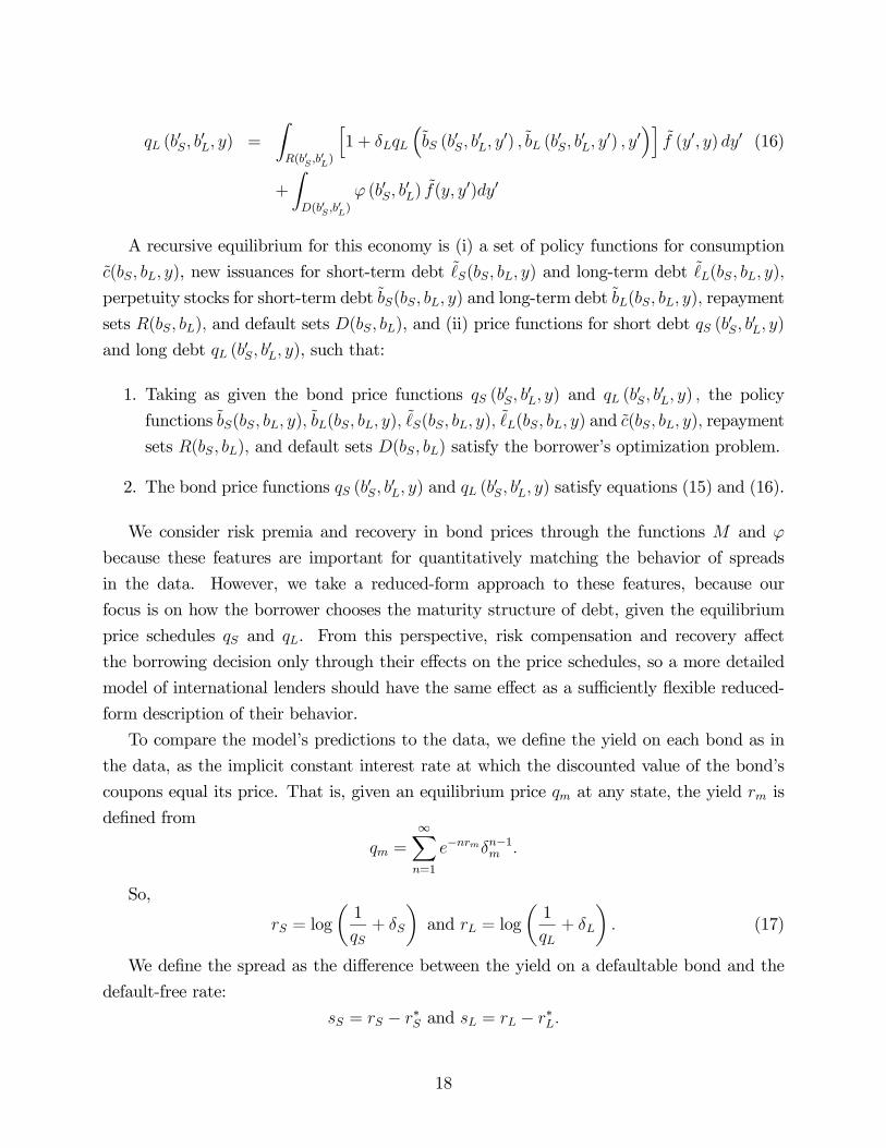
qL (b0S, b

0L, y) =

ZR(b0S ,b

0L)

h1 + δLqL

³bS (b

0S, b

0L, y

0) , bL (b0S, b

0L, y

0) , y0´i

f (y0, y) dy0 (16)

+

ZD(b0S ,b

0L)

ϕ (b0S, b0L) f(y, y

0)dy0

A recursive equilibrium for this economy is (i) a set of policy functions for consumption

c(bS, bL, y), new issuances for short-term debt S(bS, bL, y) and long-term debt L(bS, bL, y),

perpetuity stocks for short-term debt bS(bS, bL, y) and long-term debt bL(bS, bL, y), repayment

sets R(bS, bL), and default sets D(bS, bL), and (ii) price functions for short debt qS (b0S, b0L, y)

and long debt qL (b0S, b0L, y), such that:

1. Taking as given the bond price functions qS (b0S, b

0L, y) and qL (b

0S, b

0L, y) , the policy

functions bS(bS, bL, y), bL(bS, bL, y), S(bS, bL, y), L(bS, bL, y) and c(bS, bL, y), repayment

sets R(bS, bL), and default sets D(bS, bL) satisfy the borrower’s optimization problem.

2. The bond price functions qS (b0S, b0L, y) and qL (b

0S, b

0L, y) satisfy equations (15) and (16).

We consider risk premia and recovery in bond prices through the functions M and ϕ

because these features are important for quantitatively matching the behavior of spreads

in the data. However, we take a reduced-form approach to these features, because our

focus is on how the borrower chooses the maturity structure of debt, given the equilibrium

price schedules qS and qL. From this perspective, risk compensation and recovery affect

the borrowing decision only through their effects on the price schedules, so a more detailed

model of international lenders should have the same effect as a sufficiently flexible reduced-

form description of their behavior.

To compare the model’s predictions to the data, we define the yield on each bond as in

the data, as the implicit constant interest rate at which the discounted value of the bond’s

coupons equal its price. That is, given an equilibrium price qm at any state, the yield rm is

defined from

qm =∞Xn=1

e−nrmδn−1m .

So,

rS = log

µ1

qS+ δS

¶and rL = log

µ1

qL+ δL

¶. (17)

We define the spread as the difference between the yield on a defaultable bond and the

default-free rate:

sS = rS − r∗S and sL = rL − r∗L.

18

The default-free rates r∗m are the analogues of (17) defined from the prices of default-free

bonds.

As output and debt change, the probability of default varies over time, and therefore

the prices of long-term and short-term debt differ, since they each put different weights on

repayment probabilities in the future, as seen in (13). Spreads on short-term and long-term

bonds therefore generally differ, and the relationship between the two spreads changes over

time, so that the spread curve is time-varying.

Finally, we define the duration of debt issued at each date as the weighted average of the

time until each coupon payment, with the weights determined by the fraction of the bond’s

value on each payment date:

dm =1

qm

∞Xn=1

ne−nrmδn−1m .

So,

dS =1

1− δSe−rSand dL =

1

1− δLe−rL. (18)

4 Default and Optimal Maturity

In this section we illustrate the mechanisms that determine the maturity composition of debt

in a simplified, three-period version of our model, in which the borrower receives income

over time, but prefers to consume sooner rather than later. In this environment, debt allows

the borrower to transfer income between states of the world, particularly from future states

to the present, and the price of debt is determined by the borrower’s willingness to repay.

We show that short-term debt is more effective than long-term debt at transferring income

from the near future to the present. However, long-term debt allows the borrower to avoid

rolling over large short-term loans at unfavorable prices, which allows resources to be more

efficiently transferred from high-income to low-income states. We use this example to derive

statistics that are useful in measuring the relative benefits of short-term and long-term debt

in our quantitative results in the next section.

The three periods are labelled t = 0, 1, 2. The borrower’s preferences are linear over

consumption in each period, given by

U = E[c0 + βc1 + β2c2] ,

with β < 1, so that the borrower prefers to front-load consumption. In period 0, the bor-

rower’s income equals zero, and in periods 1 and 2 income y1 and y2 can take on one of two

19

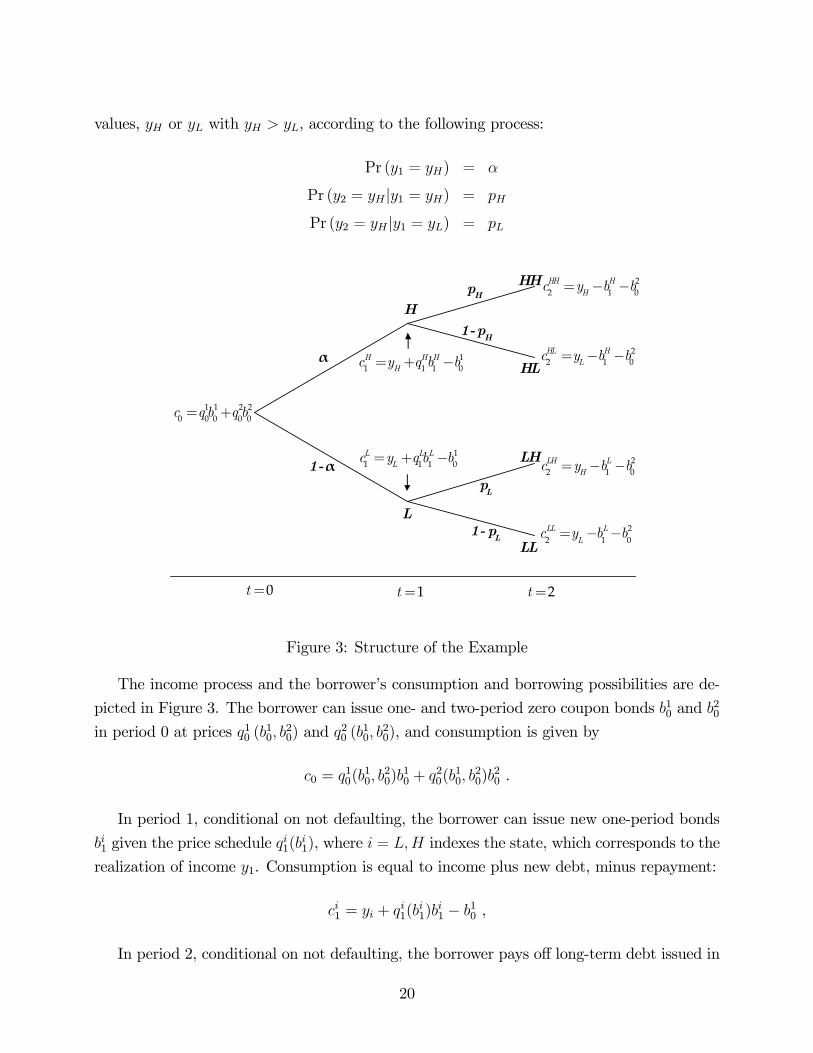
values, yH or yL with yH > yL, according to the following process:

Pr (y1 = yH) = α

Pr (y2 = yH |y1 = yH) = pH

Pr (y2 = yH |y1 = yL) = pL

 HH H

Hc y b b= − − 22 1 0

HL HLc y b b= − − 2

2 1 0

LH LHc y b b= − − 2

2 1 0

LL LL

c y b b= − − 22 1 0

H H HHc y q b b= + − 1

1 1 1 0

L

H

HH

LH

HL

LL

L L LLc y q b b= + − 1

1 1 1 0

c q b q b= +1 1 2 20 0 0 0 0

α

α1-

Hp

H1-p

Lp

L1- p

0t = 1t = 2t =

Figure 3: Structure of the Example

The income process and the borrower’s consumption and borrowing possibilities are de-

picted in Figure 3. The borrower can issue one- and two-period zero coupon bonds b10 and b20

in period 0 at prices q10 (b10, b

20) and q20 (b

10, b

20), and consumption is given by

c0 = q10(b10, b

20)b

10 + q20(b

10, b

20)b

20 .

In period 1, conditional on not defaulting, the borrower can issue new one-period bonds

bi1 given the price schedule qi1(b

i1), where i = L,H indexes the state, which corresponds to the

realization of income y1. Consumption is equal to income plus new debt, minus repayment:

ci1 = yi + qi1(bi1)b

i1 − b10 ,

In period 2, conditional on not defaulting, the borrower pays off long-term debt issued in

20

period 0 and short-term debt issued in period 1, and consumption equals income minus the

repayment:

cij2 = yj −¡bi1 + b20

¢,

where cij2 refers to consumption in the state with income history y1 = yi, y2 = yj, for i, j =

L,H. We refer to states L and H in period 1 and states LL, LH, HL, and HH in period 2.

If the borrower defaults at any time, all outstanding debt is erased and consumption from

then on is equal to ydef = 0. We assume that if the borrower is indifferent between defaulting

and repaying, then he repays. Lenders are risk-neutral and do not discount the future, and

they do not recover anything in case of default, i.e. the pricing kernelM = 1 and the recovery

rate ϕ = 0, so the price of a loan is equal to the probability or repayment.

We assume throughout this section that parameters satisfy:

pHyH − yLpH (yH − yL)

< β <

µpHyH − yLpH (yH − yL)

¶1/2(19)

This restriction ensures that the borrower is sufficiently impatient so as to borrow enough

that default happens with positive probability, but also patient enough so as to value the

future resources lost from defaulting. Under this assumption, the optimal, time-consistent

policy for the borrower is to default in period 2, only after two low shocks, i.e. in state LL,

and to repay in all other states. Bond prices on loans that are consistent with this default

policy are:

q10 = 1, q20 = α+ (1− α) pL (20)

qH1 = 1, qL1 = pL

In period 0, the borrower uses long-term debt to transfer income yL to period 0, b20 = yL.

This is because any two-period loan above yL will not be repaid in state HL, violating the

default policy. This leaves the borrower in period 1 with the ability to borrow additional

income, up to what is consistent with the default policy, from period 2, bH1 = yL − b20 = 0

and bL1 = yH − b20 = yH − yL. This implies that in period 0, the borrower is able to issue

one-period bonds b10 = yL + pL (yH − yL). The consumption allocation this implies is then

c0 = yL + pL (yH − yL) + (α+ (1− α) pL) yL (21)

cH1 = (yH − yL) (1− pL) , cL1 = 0

cHH2 = yH − yL, cHL

2 = 0

cLH2 = 0, cLL2 = ydef = 0

21

To evaluate the role each maturity of debt plays in getting to this consumption allocation,

we consider what happens if either short-term or long-term debt is reduced.

Short-term debt induces repayment in the near future To illustrate the benefit

of short-term debt, we consider what would happen if the borrower substituted long-term

debt for short-term debt in period 0. Increasing long-term debt b20 by any amount above yLrequires either defaulting in state HL as well as LL, or requires saving in period 1 to repay

the higher debt in period 2. However, saving is not optimal from the perspective of period

1, so the borrower cannot commit to saving. In equilibrium, debt issued in either state in

period 1 is nonnegative. The higher default probability lowers the price lenders are willing

to pay for long-term bonds to q20 = αpH + (1− α) pL from the value in (20), α+ (1− α) pL.

Furthermore, increasing b20 above yH is infeasible, since then q20 would drop to zero, because

of the inability to commit to saving in period 1. This means that the borrower is unable

to transfer income from either state in period 1 to period 0, because long-term borrowing is

limited by period-2 income.

In contrast, with short-term debt, the borrower is required to repay the income y1 in

the first period before borrowing against period 2 income. Since the borrower would value

the resources lost from defaulting in period 1, short-term debt is a way to use the threat of

punishment to enforce repayment in the short-term.

Long-term debt provides hedging Now we consider what would happen if the borrower

tried to substitute short-term debt for long-term debt in the original allocation. This is

infeasible because the borrower is unable to rollover any more short-term debt in period 1

state L. Under the optimal allocation derived above, consumption at all the nodes from

period 1 state L onward — cL1 , cLH2 , and cLL2 in (21) — are zero, so any additional debt due in

period 1 state L cannot be repaid.

Long-term debt helps the borrower in this situation because it provides a hedge against

the uncertainty in period 1. To see how this works, consider the resources available for

consumption in period 1. Given that bH1 = yL − b20 and bL1 = yH − b20, consumption in period

1 is given by:

cH1 = yH − b10 +¡yL − b20

¢cL1 = yL − b10 + pL

¡yH − b20

¢Decreasing b10 in favor of increasing b20 reduces the present value of the borrower’s debt

obligations — how much debt needs to be rolled over — in the low-income state, but leaves

22

it unchanged in the high-income state. In this sense, issuing long-term debt is a hedge. In

effect, issuing long-term debt transfers resources from state H to state L, since increasing b20lowers cH1 at a one-to-one rate, while it lowers c

L1 at the rate pL < 1. This raises the value of

resources at the rate (1− pL). Since the borrower prefers to consume early, this transfer of

income out of state H in period 1 changes consumption relative to the allocation with only

one-period bonds by raising consumption in period 0 (by the present value α (1− pL) yL).

Equilibrium consumption and default with only one maturity of debt The previ-

ous two subsections illustrated that short-term and long-term debt provide distinct benefits,

in the sense that the borrower cannot costlessly substitute one for the other. For complete-

ness, we provide here the optimal allocations with only one maturity of debt. With only

long-term debt, the borrower defaults in the additional state (HL) in period 2. With only

short-term debt, though, the borrower does not actually borrow enough to face a roll-over

crisis and default in period 1 state L; borrowing is simply constrained in period 0.

The allocations with only one maturity of debt are as follows:

Only long-term debt Only short-term debt

b20 = yH b10 = yL + pLyH

bL1 = 0, bH1 = 0 bL1 = yH , bH1 = yL

c0 = (αpH + (1− α) pL) yH c0 = yL + pLyH

cH1 = yH , cL1 = yL cH1 = (1− pL) yH , cL1 = 0

cHH2 = 0, cHL

2 = ydef = 0 cHH2 = yH − yL, cHL

2 = 0

cLH2 = 0, cLL2 = ydef = 0 cLH2 = 0, cLL2 = ydef = 0

It is straightforward to show that the borrower attains strictly lower utility under either of

these allocations than under the consumption allocation in (21) with both short-term and

long-term debt.

Summary

In a standard incomplete markets model with fluctuating output and without default, a

borrower would find the portfolio of long and short debt indeterminate if the risk-free rate

were constant across time; the two assets would have payoffs that make them equivalent.

However, in our model, the risk of default makes the two assets distinct, resulting in a tradeoff

between issuing short-term and long-term debt. This tradeoff in our example is similar to

that analyzed in Hart and Moore (1989, 1994), in a contracting problem between an investor

and an entrepreneur who controls a productive project. Hart and Moore argue that the

23

tension between short-term and long-term debt is between defaulting early or defaulting

later, but with larger losses. In our example, this tension limits the capacities of short-term

and long-term borrowing differently.

The capacity for borrowing using long-term debt is limited by the inability to commit to

saving income in the near future to repay farther in the future. Hence short-term debt is

a better instrument for borrowing against resources in the near future, because large short-

term loans are available at higher prices than long-term loans. We refer to this benefit

as a liquidity advantage of short-term debt. However, the borrowing capacity of short-

term debt is limited by the risk of not being able to roll over large amounts of short-term

debt in low-income states. Long-term debt alleviates this problem by enabling a transfer

of resources from high-income states to low-income states. We call this attribute a hedging

benefit of long-term debt, because the outstanding value of long-term debt falls in states

of the world in which resources are scarce. In our examples above, this hedging translated

into higher current consumption, because we assumed the borrower did not value smoothing

consumption across states; however, if the borrower were risk averse, long-term debt would

enable smoothing consumption across states through this hedging benefit. This hedging

mechanism is essentially the same as the role of long-lived securities in allocating risk across

periods in Kreps (1982). Angeletos (2002), Buera and Nicolini (2004), and Lustig, Sleet, and

Yeltekin (2008) emphasize this mechanism in models of the optimal maturity structure of

government debt with incomplete markets. The difference in our model is that bond prices

vary across states — and hence provide hedging — due to the government’s inability to commit

to repaying, even in the absence of variation in the lender’s marginal rate of substitution.

These liquidity and hedging properties shape the optimal maturity structure of debt

when the borrower can default. The quantitative relevance of each of these forces depends

on the specifics of preferences and the income process. Thus, in the next section we quantify

these two effects by calibrating our general model to an actual emerging market economy.

To measure the liquidity and hedging mechanisms in our quantitative results in the next

section, we use two simple measures that follow from the examples in this section. The

liquidity advantage of short-term debt is reflected in its higher price and the ability to increase

current consumption more than what is possible with long-term debt. The hedging advantage

of long-term debt can be captured in the higher volatility of the value of outstanding long-

term debt relative to short-term debt. The example above illustrates an extreme version of

this: the value of short-term debt does not vary at all. Since the value of long-term debt

varies more, it provides a better hedge than short-term debt.

24

5 Quantitative Analysis

5.1 Parameterization

We solve the model numerically to evaluate its quantitative predictions regarding the dynamic

behavior of the optimal maturity composition of debt and the spread curve in emerging

markets. We calibrate an annual model to the Brazilian economy.15

The utility function of the borrower is u(c) =c1−σ

1− σ. The borrower’s risk aversion coeffi-

cient is set to 2, which is a common value used in real business cycle studies. The stochastic

process for output is a log-normal AR(1) process, log(yt+1) = ρ log(yt)+εt+1 with E[ε2] = η2.

We discretize the shocks into a six-state Markov chain using a quadrature-based procedure

(Tauchen and Hussey, 1991). We use annual series of GDP growth for 1960—2004 taken from

the World Development Indicators to calibrate the volatility of output. Due to the short

sample, rather than estimating the autocorrelation coefficient we choose an autocorrelation

coefficient for the output process of 0.9, which is in line with standard estimates for developed

countries. The decay parameters of the short and long bonds, δS and δL, are set such that

the default-free durations equal 2 and 10 years. We also choose the probability of reentering

financial markets, θ, so that the average length of time in exclusion is 6 years, consistent

with data presented in Benjamin and Wright (2009) on the median length of sovereign debt

renegotiations.

The function ϕ (bS, bL) in the pricing expressions (15)-(16) is a reduced-form represen-

tation of the fraction of debt recovered after default. We set this function to ϕ (bS, bL) =

exp (− (q∗SbS + q∗LbL)), with q∗S and q∗L equal to the default-free prices. This functional form

is a convenient way to capture two features of the recovery rate: it lies between zero and one,

and it declines with the quantity of debt issued. Intuitively, this is motivated by the idea

that there is a fixed amount of surplus that lenders are able to extract from borrowers in the

event of a default, so this amount declines as a fraction of debt as debt grows. Yue (2006)

shows that, in a model in which the debt recovery rate is endogenously determined by a bar-

gaining process between lenders and a defaulting borrower, the recovery rate is decreasing

and convex in debt, much like the function ϕ.

The risk premium in our model comes from the interaction of the lenders’ pricing kernel

with default outcomes. We can rewrite equation (15) (and analogously, (16)) as a typical

15The algorithm used to solve the model extends that in Arellano (2009) to allow for two bonds. Inaddition, we follow Hatchondo, Martinez and Sapriza (2009) in updating the value function and the bondprice functions concurrently.

25

asset-pricing equation:

qS = E [M 0x0S]

where

x0S =

(1 + δSq

0S in states in which the borrower repays

ϕ in states in which the borrower defaults

Written this way, the price of a bond is composed of the lender’s discounted expected

payoff plus a risk premium term:

qS = E [M 0]E [x0S] + cov (M 0, x0S)

Payoffs vary across states due to default events as well as changes in the future probability

of default, reflected in q0S. To the extent that this variation is negatively correlated with the

pricing kernel, investors are compensated for this risk through paying a lower price qS for

debt. We specify the pricing kernel as follows:

M (yt, yt+1) = exp

µ−r − αεt+1 −

1

2α2η2

¶(22)

where r and α are parameters, εt+1 = log yt+1−ρ log yt is the shock to the borrower’s income,and η is its variance. The term r represents the risk-free interest rate; we set this at 4%

annually, which equals the average annual yield of a two year U.S. bond from 1996 to 2004.

The term α controls correlated the pricing kernel is with innovations εt+1 to the borrower’s

income level. (The term 12α2η2 is a normalization.)

This pricing kernel is a variation on the one-factor term structure models discussed in,

for example, Backus, Foresi, and Telmer (1998). We define the pricing kernel as a function

of only the borrower’s income because it is a parsimonious way to model risk premia that

vary with the probability of default. In our model, default decisions depend on the model’s

entire state, (y, bS, bL), but our shortcut is valid for two reasons: first, default probabilities

in the model are highly correlated with income. Second, in the absence of default, our model

with this pricing kernel would generate a default-free interest rate that is constant and a flat

default-free term structure. This is because, from equations (15) or (16), the price q∗m of a

26

default-free m-duration bond is given by16:

q∗m =

Z(1 + δmq

∗m)M (y, y0) f (y0, y) dy0 (23)

=e−r

1− δme−r

so the yield, defined as in equation (17), is constant and independent of the bond’s duration:17

r∗m = log

µ1

q∗m+ δm

¶= r

Even though α is a constant, the size of the risk premium varies over time because the

default probability, which depends on y, bS, and bL, varies over time. The borrower’s income

is a convenient state variable, because the borrower tends to default when income is low.

Since income is persistent, low current income signals high default probabilities, and hence

low prices, in the future. Therefore, since payoffs xm are positively correlated with the

borrower’s income, the pricing kernel M in equation (22) generates a positive risk premium

if α > 0.

We calibrate the parameter α as well as the output cost after default, λ, and the borrower’s

time preference parameter β, to match the following moments of Brazilian data: the average

2- and 10-year spreads and the volatility of the trade balance relative output.

Table 4 summarizes the parameter values, and Table 5 presents the calibrated moments

as well as other statistics from the model. The model matches the calibrated moments well,

although it underestimates a bit the mean 10-year spread. The model predicts that con-

sumption is about as variable as output, and that consumption is negatively correlated with

spreads and the fraction of debt that is short term: in bad times, consumption is low, spreads

are relatively high, and debt is mostly short. The high volatility of consumption relative to

output and the countercyclicality of spreads are well documented features of emerging mar-

kets. The model predicts that the average recovery in default is 44%, as compared to the

16Using the fact that M is lognormal,

E [M (y, y0) |y] = exp

µE [logM (y, y0) |y] + 1

2var [logM (y, y0) |y]

¶= exp (−r)

17In practice, since we discretize the state space of our model, we also have to normalize the pricing kernelso that default-free yields are constant in the discretized environment.

27

average recovery rate of 60% reported in sovereign defaults reported by Benjamin and Wright

(2009).

Table 4: Parameters ValuesValue Target

Lenders’ discount rate r = 4% U.S. annual interest rate 4%Borrower’s risk aversion σ = 2 Standard valuePerpetuity decay factors δS = 0.52 Default-free durations of 2 and 10 years

δL = 0.936Stochastic structure ρ = 0.9, η = 0.017 Brazil outputProbability of reentry θ = 0.17 Benjamin and Wright (2009)Calibrated parametersLenders’ pricing kernel

Output after defaultBorrower’s discount factor

α = 1.3λ = 0.22β = 0.932

⎫⎬⎭ Brazil average 2-year spreadBrazil average 10-year spreadvolatility of trade balance

Table 5: Model StatisticsModel Data

Targeted Momentsmean sS (percent) 5.5 5.6mean sL (percent) 6.4 7.1std(trade balance)/std(y) 0.36 0.36Other Momentsmean recovery rate 0.44 0.60std(c)/std(y) 1.01 1.10corr(c,2-year spread) -0.42corr(c,10-year spread) -0.34corr(c, qS S/(qS S + qL L)) -0.77

5.2 Results

We simulate the model, and in the following subsections we report statistics on the dynamic

behavior of spreads and the maturity composition of debt from the limiting distribution of

debt holdings. We first show that the model matches the data in generating time-varying

differences in the pricing of short- and long-term debt, due to movements in the probability of

default and risk premia. The behavior of prices generates time-varying liquidity and hedging

benefits of the two assets, which rationalizes the maturity composition observed in the data.

28

Prices and Spreads

Default in our model happens when the economy has a low level of wealth, either due to

low income or high debt. Since income and debt are persistent, states with low income and

high debt tend to have high spreads, as the future probabilities of default, and therefore risk

premia, are high.

We now compare spread dynamics in the model to the data. The series for the data are

Brazilian 2- and 10-year spreads and prices from Section 2. For this comparison, we organize

the data into quantiles based on the level of the short spread. Table 6 presents average spreads

for short and long debt as well as the risk premium component of the model’s spreads across

periods when short spreads are below their 25th and 50th percentiles and above their 50th

and 75th percentiles.

Table 6: Spread CurvesDATA MODEL

sS percentile sS sL sS sL rpS rpL< 25 2.2 5.3 0.6 2.6 0.2 0.4< 50 2.7 5.4 1.2 3.4 0.3 0.5≥ 50 8.5 8.9 9.7 9.5 0.5 0.7≥ 75 12.3 10.8 14.9 14.0 0.7 0.9Mean 5.6 7.1 5.5 6.4 0.4 0.6

The first two columns of Table 6 present the short and long spreads in the data, and the

last four columns present the model’s predictions. In the model, when default is unlikely,

both spreads are low, and the spread curve is upward-sloping: when the short spread is below

its 25th percentile, for example, the average short spread is 0.6%, and the average long spread

is 2.6%. In contrast, when the probability of default is higher, both spreads rise, and the

spread curve becomes downward-sloping: when the short spread is above the 75th percentile,

the average short spread is 14.9%, and the average long spread is 14.0%. Compared to the

data for Brazil, the model captures well the dynamics of spreads curves and in particular the

slope of the spread curve associated with periods of high and low spreads. When spreads

are below the 25th percentile, the slope is about 2 percentage points, compared to a slope

of 3 percentage points in Brazil. In periods with spreads above the 75th percentile, the

slope of the spread curve in the model inverts to −0.9 percentage points, compared to −1.5percentage points in Brazil. The model also generate an average slope of the spread curve of

about 1 percentage point, compared to 1.5 percentage points in the Brazilian data.

29

Our model provides a decomposition of interest rate spreads into two parts: the actuarially

fair compensation for expected losses from default, and the risk premium. The actuarially

fair price qAFm of a bond of duration m is defined by taking the bond pricing equations (15)-

(16) and substituting just the probability density, f , for the product of the pricing kernel

and probability density, f :

qAFm (b0S, b0L, y) =

ZR(b0S ,b

0L)

h1 + δmq

AFm

³bS (b

0S, b

0L, y

0) , bL (b0S, b

0L, y

0) , y0´i

f (y0, y) dy0

+

ZD(b0S ,b

0L)

ϕ (b0S, b0L) f(y, y

0)dy0,

Then, the actuarially fair yield is given by rAFm = log¡1/qAFm + δm

¢, and the spread risk

premium is defined as rpm = rm−rAFm . The fifth and sixth columns of Table 6 show the term

structure of spread risk premia in the model. Risk premia are positive, because the borrower

tends to default in states with low income, and the lender’s pricing kernel M is negatively

correlated with income. Also, risk premia are generally small according to this measure,

averaging less than one percentage point. However, they make up a relatively large fraction

of the interest rate spreads in good times, when the spreads are low. For example, the risk

premium accounts for one third of the 2-year spread when 2-year spreads are below their

25th percentile, but only for five percent when 2-year spreads are above their 75th percentile.

In addition, the risk premium on long-term debt is always higher than on short-term debt,

reflecting the fact that the risk premium is cumulated over a longer horizon. In effect, our

model says that risk premia do not need to increase a lot in bad times to account for the large

increases in spreads, because the expected probability of default rises so much. However, this

decomposition does not address the question of how the degree of required risk compensation

affects debt and default choices, and in turn the equilibrium term structure of spreads. We

examine this question in more detail in subsection 5.3.

Much of the literature on empirical asset pricing focuses on returns as a measure of risk

premia. In the context of sovereign bonds, Broner, Lorenzoni, and Schmukler (2008) show

that excess returns — returns relative to default-free bonds — on long-term bonds rise more

than excess returns on short-term bonds during a crisis, i.e. when spreads rise. Computing

excess returns from our model’s simulated data generates this pattern as well. Specifically, we

find that the average excess returns, defined as (1+δmq0m)/qm− (1+r), equal 0.3% and 0.4%

for short and long-term bonds in periods when the short spread is below its median. These

returns increase to 7.9% and 10.4% respectively when the short spread is above its median.

In our model, however, average excess returns in a simulation also capture changes in default

30

probabilities, not just risk premia. In fact, under actuarially fair pricing, the magnitude and

pattern of average excess returns are similar to those under pricing with risk premia. We

choose not to focus on average excess returns, because in our model they are not zero in the

absence of risk premia.

Underlying the time-varying spreads is the interaction of the dynamics of income and debt

with the price schedules for short and long debt. (Figure 4, in the Appendix, illustrates the

equilibrium price schedules for short debt qS(b0S, b0L, y) and long debt qL(b

0S, b

0L, y).) However,

the mapping from discount prices to spreads is not linear (eq. 1). Thus, it is informative

to analyze price ratios defined as defaultable discount prices relative to default-free prices

for a bond with duration m: qm/q∗m. The price ratio of each bond is the total discounted

repayment probability over the lifetime of the bond, adjusted for risk and recovery. Table

7 presents statistics for these price ratios in the model and the data. The table shows that

contrary to spreads, price ratios for short-term debt are always higher than for long-term

debt both in the model and in the data. Moreover, price ratios are disproportionately lower

for long-term debt when spreads are high, both in the model and in the data.18

Table 7: PricesDATA MODEL

sS pct qS/q∗S qL/q

∗L qS/q

∗S qL/q

∗L

< 25 0.96 0.60 0.99 0.79< 50 0.95 0.59 0.98 0.75≥ 50 0.85 0.43 0.85 0.57≥ 75 0.79 0.35 0.79 0.48Mean 0.90 0.51 0.91 0.66

The distinct dynamics of price ratios and spreads can be understood as follows. Price

ratios reflect cumulative repayment probabilities adjusted for risk and recovery, whereas

spreads reflect average default probabilities. Cumulative default risk for long-term debt is

always larger than for short-term debt both in the data and the model. However, annualized

(average) default risk can be lower on long-term debt during times when the annual default

probability in the short run is larger than the annual default probability in the long run.

Thus, contrary to common belief in sovereign debt markets, the interest rate spread is not a

comprehensive measure of the relative cost of borrowing across different maturities of debt.

In particular, in times when the probability of default is high, short-term debt may appear

18These patterns hold for price ratios in the data for Argentina, Mexico, and Russia as well.

31

to be more expensive than long-term debt, in the sense that it has a higher spread, although

long-term debt is worse in the sense that it has a lower price, relative to the risk-free price.

The connection between the dynamic behavior of prices and spreads in our model is borne

out in the data as well.

The preceding discussion also indicates that the important feature of our model for gener-

ating the observed dynamics of prices and the spread curve is that the probability of default

is mean-reverting: a period with high probability of default is followed by a period with lower

probability of default, and vice versa. The effects of mean-reverting default probabilities on

the spread curve are the same as those highlighted by Merton (1974) in the case of credit

spreads for corporate debt. In our model the probability of default is endogenously mean-

reverting as a result of the dynamics of the output process and debt accumulation. When

output is high, it is also expected to be high in the near future, so the probability of default in

the next period is low. The economy borrows a large amount at low interest rate spreads, so

that in states where the economy is hit by a bad shock, default becomes more likely further in

the future. In contrast, when the likelihood of imminent default is high, the economy avoids

default in the next period only in states with high output. Conditional on not defaulting,

then, output is expected to remain high, and the probability of default further in the future

falls. The persistence and mean reversion of default and repayment probabilities driven by

the dynamics of debt and income therefore rationalize the dynamic behavior of the spread

curve observed in the data.

Maturity Composition

We now present the quantitative predictions for the maturity composition of debt. As dis-

cussed in Section 4, the benefits of short and long-term debt shape the dynamic behavior

of the maturity composition. First, long-term bonds provide a hedge that prevents having

to roll-over large amounts of debt at low prices; we find that this hedging motive is more

valuable in times of high wealth. Second, short-term bonds are better at solving the lack

of enforcement problem as they reduce the default likelihood and are less likely to require

savings in order to be repaid. These forces give short-term debt the liquidity advantage as

more resources can be transferred to the present; we find that this liquidity motive is more

valuable in times of low wealth. Given the negative correlation between wealth and spreads,

the borrower in our model uses long-term debt more heavily in times when spreads are low

and shifts toward shorter term debt when spreads are high.

32

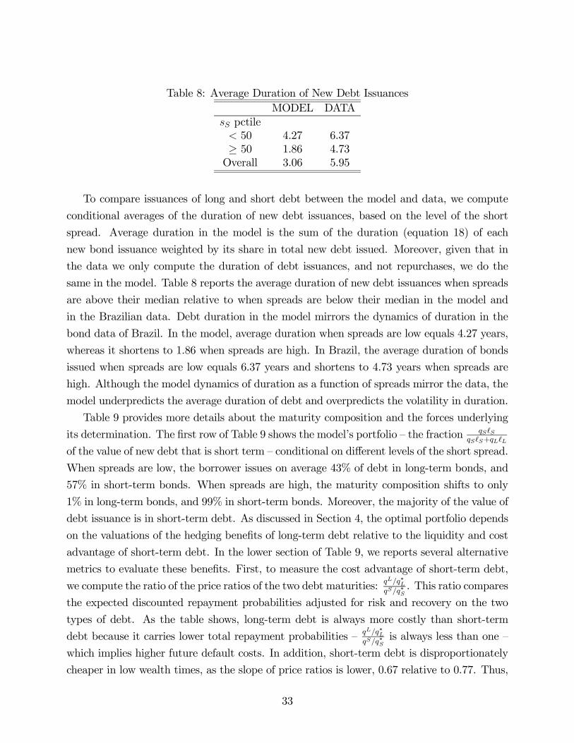
Table 8: Average Duration of New Debt IssuancesMODEL DATA

sS pctile< 50 4.27 6.37≥ 50 1.86 4.73Overall 3.06 5.95

To compare issuances of long and short debt between the model and data, we compute

conditional averages of the duration of new debt issuances, based on the level of the short

spread. Average duration in the model is the sum of the duration (equation 18) of each

new bond issuance weighted by its share in total new debt issued. Moreover, given that in

the data we only compute the duration of debt issuances, and not repurchases, we do the

same in the model. Table 8 reports the average duration of new debt issuances when spreads

are above their median relative to when spreads are below their median in the model and

in the Brazilian data. Debt duration in the model mirrors the dynamics of duration in the

bond data of Brazil. In the model, average duration when spreads are low equals 4.27 years,

whereas it shortens to 1.86 when spreads are high. In Brazil, the average duration of bonds

issued when spreads are low equals 6.37 years and shortens to 4.73 years when spreads are

high. Although the model dynamics of duration as a function of spreads mirror the data, the

model underpredicts the average duration of debt and overpredicts the volatility in duration.

Table 9 provides more details about the maturity composition and the forces underlying

its determination. The first row of Table 9 shows the model’s portfolio — the fraction qS S

qS S+qL L

of the value of new debt that is short term — conditional on different levels of the short spread.

When spreads are low, the borrower issues on average 43% of debt in long-term bonds, and

57% in short-term bonds. When spreads are high, the maturity composition shifts to only

1% in long-term bonds, and 99% in short-term bonds. Moreover, the majority of the value of

debt issuance is in short-term debt. As discussed in Section 4, the optimal portfolio depends

on the valuations of the hedging benefits of long-term debt relative to the liquidity and cost

advantage of short-term debt. In the lower section of Table 9, we reports several alternative

metrics to evaluate these benefits. First, to measure the cost advantage of short-term debt,

we compute the ratio of the price ratios of the two debt maturities: qL/q∗LqS/q∗S

. This ratio compares

the expected discounted repayment probabilities adjusted for risk and recovery on the two

types of debt. As the table shows, long-term debt is always more costly than short-term

debt because it carries lower total repayment probabilities — qL/q∗LqS/q∗S

is always less than one —

which implies higher future default costs. In addition, short-term debt is disproportionately

cheaper in low wealth times, as the slope of price ratios is lower, 0.67 relative to 0.77. Thus,

33

a larger share of short-term debt in low wealth times can be understood as a reaction to the

more expensive long-term debt.

Table 9: Model Maturity CompositionShort Spread

< 50 pctile ≥ 50 pctile overall meanqS S / (qS S + qL L) 0.57 0.99 0.79

sS, percent 1.2 9.7 5.5

sL − sS, percent 2.2 -0.3 1.0

(qL/q∗L) / (qS/q

∗S) 0.77 0.67 0.72

∆S / ∆L 1.43 1.67 1.46

std(value debt)

⎧⎪⎨⎪⎩short

long

total

0.25

1.08

0.93

0.69

0.03

0.71

0.60

0.89

0.83

std(price debt)

(short

long

0.09

0.79

0.21

1.21

0.18

1.17

corr(value debt, y0)

⎧⎪⎨⎪⎩short

long

total

-0.45

0.72

0.75

0.83

0.15

0.83

-0.06

0.70

0.72

A more detailed measure of the liquidity benefit of short-term debt is given by calculating

the increase in consumption that would be possible by marginally increasing short-term debt,

relative to the increase in consumption that is possible by issuing more long-term debt.

Specifically, define Ψ(b0S, b0L, bS, bL, y) ≡ qS(b0S, b

0L, y)(b

0S − δSbS) + qL(b0S, b

0L, y)(b

0L − δLbL) as

the quantity of consumption that is attained with a certain debt policy b0S, b0L, given the

state (bS, bL, y). We calculate the ratio of deviations from the equilibrium debt policy for

short-term debt relative to long-term debt,

∆S

∆L≡ Ψ(b0S + εS, b

0L, bS, bL, y)−Ψ(b0S, b

0L, bS, bL, y)

Ψ(b0S, b0L + εL, bS, bL, y)−Ψ(b0S, b

0L, bS, bL, y)

where εS and εL are small, and are chosen so that if bond prices were always equal to the

default-free prices, the ratio would be exactly equal to 1. This ratio in our model is on average

equal to 1.46. Thus, short-term debt is in equilibrium more liquid because consumption can

be marginally increased more with short-term debt than with long-term debt. The reason

is that price schedules for short-term debt are more lenient by having higher prices that

34

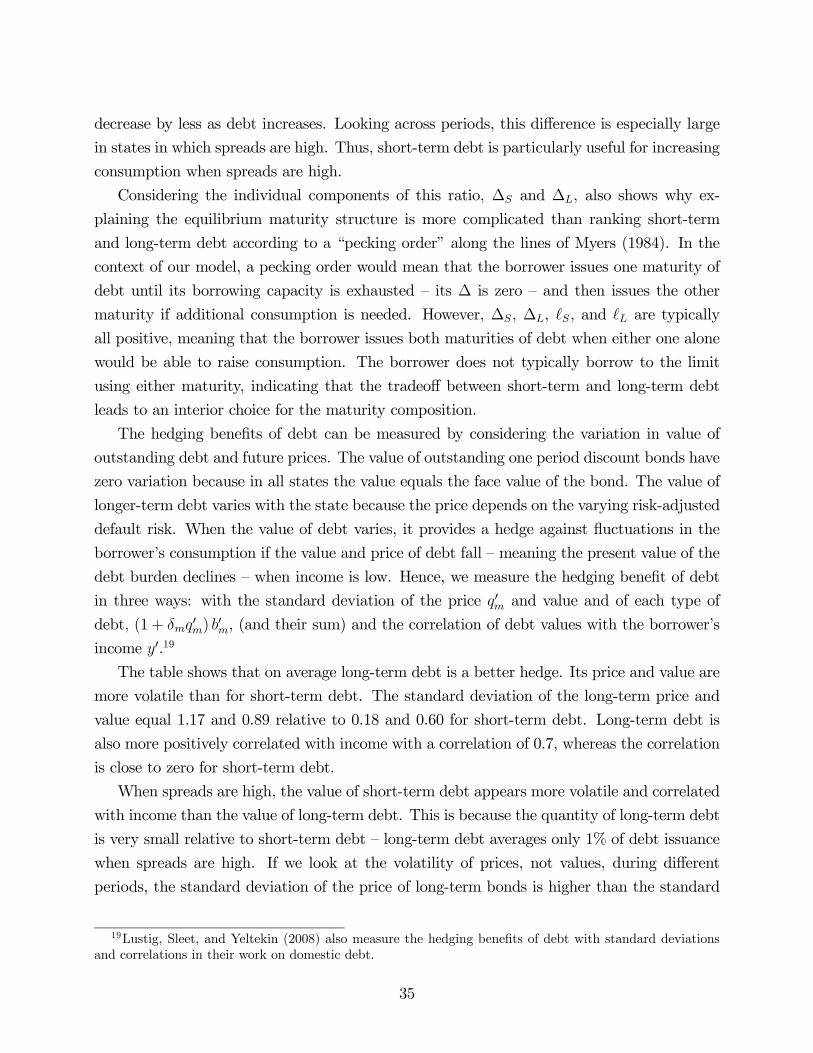
decrease by less as debt increases. Looking across periods, this difference is especially large

in states in which spreads are high. Thus, short-term debt is particularly useful for increasing

consumption when spreads are high.

Considering the individual components of this ratio, ∆S and ∆L, also shows why ex-

plaining the equilibrium maturity structure is more complicated than ranking short-term

and long-term debt according to a “pecking order” along the lines of Myers (1984). In the

context of our model, a pecking order would mean that the borrower issues one maturity of

debt until its borrowing capacity is exhausted — its ∆ is zero — and then issues the other

maturity if additional consumption is needed. However, ∆S, ∆L, S, and L are typically

all positive, meaning that the borrower issues both maturities of debt when either one alone

would be able to raise consumption. The borrower does not typically borrow to the limit

using either maturity, indicating that the tradeoff between short-term and long-term debt

leads to an interior choice for the maturity composition.

The hedging benefits of debt can be measured by considering the variation in value of

outstanding debt and future prices. The value of outstanding one period discount bonds have

zero variation because in all states the value equals the face value of the bond. The value of

longer-term debt varies with the state because the price depends on the varying risk-adjusted

default risk. When the value of debt varies, it provides a hedge against fluctuations in the

borrower’s consumption if the value and price of debt fall — meaning the present value of the

debt burden declines — when income is low. Hence, we measure the hedging benefit of debt

in three ways: with the standard deviation of the price q0m and value and of each type of

debt, (1 + δmq0m) b

0m, (and their sum) and the correlation of debt values with the borrower’s

income y0.19

The table shows that on average long-term debt is a better hedge. Its price and value are

more volatile than for short-term debt. The standard deviation of the long-term price and

value equal 1.17 and 0.89 relative to 0.18 and 0.60 for short-term debt. Long-term debt is

also more positively correlated with income with a correlation of 0.7, whereas the correlation

is close to zero for short-term debt.

When spreads are high, the value of short-term debt appears more volatile and correlated

with income than the value of long-term debt. This is because the quantity of long-term debt

is very small relative to short-term debt — long-term debt averages only 1% of debt issuance

when spreads are high. If we look at the volatility of prices, not values, during different

periods, the standard deviation of the price of long-term bonds is higher than the standard

19Lustig, Sleet, and Yeltekin (2008) also measure the hedging benefits of debt with standard deviationsand correlations in their work on domestic debt.

35

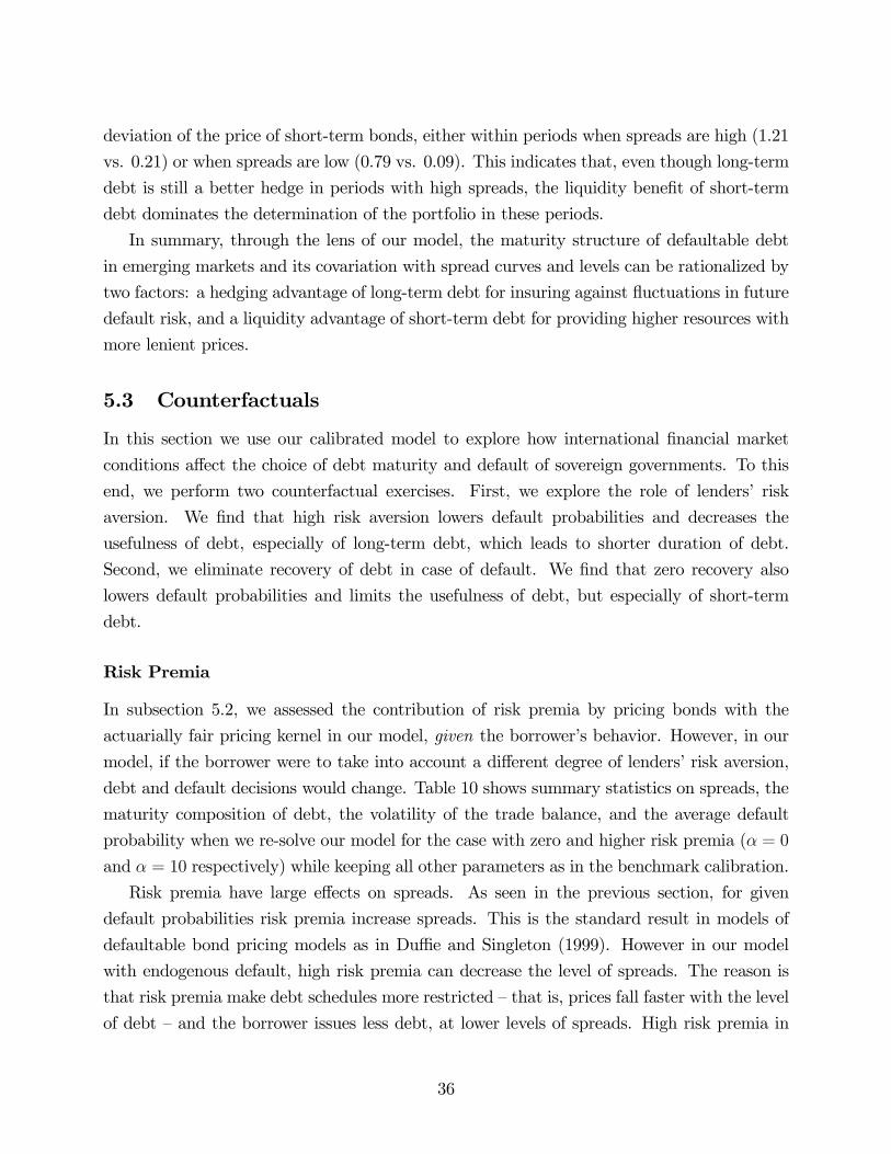
deviation of the price of short-term bonds, either within periods when spreads are high (1.21

vs. 0.21) or when spreads are low (0.79 vs. 0.09). This indicates that, even though long-term

debt is still a better hedge in periods with high spreads, the liquidity benefit of short-term

debt dominates the determination of the portfolio in these periods.

In summary, through the lens of our model, the maturity structure of defaultable debt

in emerging markets and its covariation with spread curves and levels can be rationalized by

two factors: a hedging advantage of long-term debt for insuring against fluctuations in future

default risk, and a liquidity advantage of short-term debt for providing higher resources with

more lenient prices.

5.3 Counterfactuals

In this section we use our calibrated model to explore how international financial market

conditions affect the choice of debt maturity and default of sovereign governments. To this

end, we perform two counterfactual exercises. First, we explore the role of lenders’ risk

aversion. We find that high risk aversion lowers default probabilities and decreases the

usefulness of debt, especially of long-term debt, which leads to shorter duration of debt.

Second, we eliminate recovery of debt in case of default. We find that zero recovery also

lowers default probabilities and limits the usefulness of debt, but especially of short-term

debt.

Risk Premia

In subsection 5.2, we assessed the contribution of risk premia by pricing bonds with the

actuarially fair pricing kernel in our model, given the borrower’s behavior. However, in our

model, if the borrower were to take into account a different degree of lenders’ risk aversion,

debt and default decisions would change. Table 10 shows summary statistics on spreads, the

maturity composition of debt, the volatility of the trade balance, and the average default

probability when we re-solve our model for the case with zero and higher risk premia (α = 0

and α = 10 respectively) while keeping all other parameters as in the benchmark calibration.

Risk premia have large effects on spreads. As seen in the previous section, for given

default probabilities risk premia increase spreads. This is the standard result in models of

defaultable bond pricing models as in Duffie and Singleton (1999). However in our model

with endogenous default, high risk premia can decrease the level of spreads. The reason is

that risk premia make debt schedules more restricted — that is, prices fall faster with the level

of debt — and the borrower issues less debt, at lower levels of spreads. High risk premia in

36

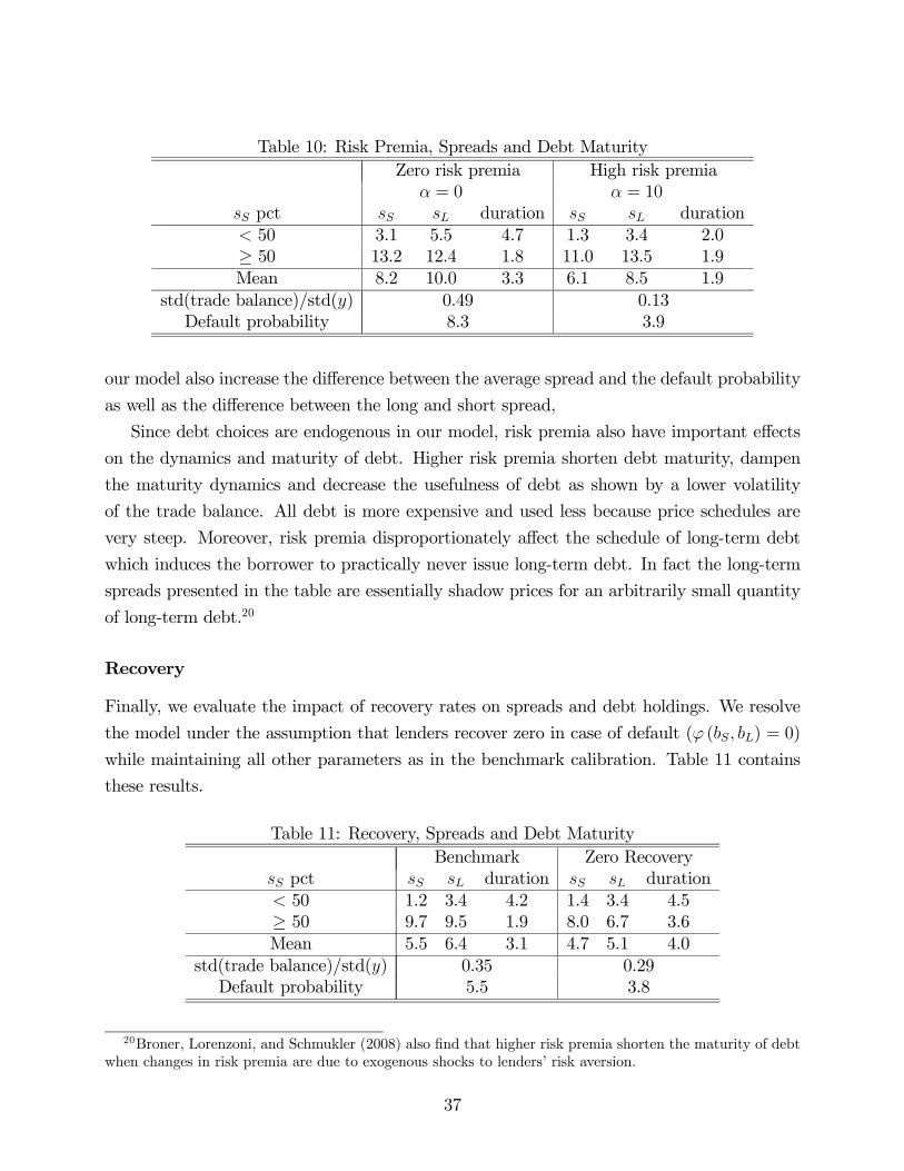
Table 10: Risk Premia, Spreads and Debt MaturityZero risk premia High risk premia

α = 0 α = 10sS pct sS sL duration sS sL duration< 50 3.1 5.5 4.7 1.3 3.4 2.0≥ 50 13.2 12.4 1.8 11.0 13.5 1.9Mean 8.2 10.0 3.3 6.1 8.5 1.9

std(trade balance)/std(y) 0.49 0.13Default probability 8.3 3.9

our model also increase the difference between the average spread and the default probability

as well as the difference between the long and short spread,

Since debt choices are endogenous in our model, risk premia also have important effects

on the dynamics and maturity of debt. Higher risk premia shorten debt maturity, dampen

the maturity dynamics and decrease the usefulness of debt as shown by a lower volatility

of the trade balance. All debt is more expensive and used less because price schedules are

very steep. Moreover, risk premia disproportionately affect the schedule of long-term debt

which induces the borrower to practically never issue long-term debt. In fact the long-term

spreads presented in the table are essentially shadow prices for an arbitrarily small quantity

of long-term debt.20

Recovery

Finally, we evaluate the impact of recovery rates on spreads and debt holdings. We resolve

the model under the assumption that lenders recover zero in case of default (ϕ (bS, bL) = 0)

while maintaining all other parameters as in the benchmark calibration. Table 11 contains

these results.

Table 11: Recovery, Spreads and Debt MaturityBenchmark Zero Recovery

sS pct sS sL duration sS sL duration< 50 1.2 3.4 4.2 1.4 3.4 4.5≥ 50 9.7 9.5 1.9 8.0 6.7 3.6Mean 5.5 6.4 3.1 4.7 5.1 4.0

std(trade balance)/std(y) 0.35 0.29Default probability 5.5 3.8

20Broner, Lorenzoni, and Schmukler (2008) also find that higher risk premia shorten the maturity of debtwhen changes in risk premia are due to exogenous shocks to lenders’ risk aversion.

37

Recovery has important effects on spreads, borrowing and default. The standard result in

models of defaultable bond pricing models is that reducing recovery rates increases spreads

because debt is discounted more heavily as the loss in case of default is larger for lenders.

However, in our model making borrowing ex-ante more expensive means that debt schedules

for short and long-term debt become more restricted which in equilibrium lowers default

because the borrower issues less debt. Hence, as in the case of high risk premia, lower

recovery rates makes spreads smaller and induces less usage of debt.

Table 11 shows that relative to the benchmark case (which produced an average recovery

rate of 44%) having zero recovery reduces default probabilities from 5.5% to 3.8% and reduces

average spreads by about 1%. In addition, zero recovery lowers the volatility of the trade

balance which implies less use of debt. Lower recovery also lengthens the debt maturity by

about a year and dampens the maturity dynamics. The reason why the model produces

a higher mean duration when recovery is zero is that an equal recovery rate for short and

long-term debt (as in the benchmark) is disproportionately beneficial for short-term debt

prices, which are on average lower than the long term price. Hence, reducing recovery rates

disproportionately restricts the short-term debt schedule and induces a shift in the portfolio

towards long term debt. The maturity dynamics are dampened because the steep schedules

restrict the liquidity and hedging benefits of short and long-term debt.

6 Conclusion

In this paper, we have developed a dynamic model to study the maturity composition of

sovereign bonds. In emerging markets data, changes in the maturity composition of debt

comove with changes in the term structure of spreads: when spreads on short-term debt are

low, long-term spreads are higher than short-term spreads, and the maturity of debt issued

is long. When short-term spreads rise, long-term spreads rise less, and the maturity of debt

shortens. Our model simultaneously reproduces the patterns observed in the term structure

of spreads and bond prices, and the maturity composition of debt. Changes in the spread

curve, which reflects the average default probability and risk premia at different time horizons,

result from the output dynamics and the endogenous dynamics of debt. Issuing long-term

debt hedges future fluctuations in consumption that come from changes in debt prices. Short-

term debt provides more liquidity because it allows the borrower to avoid the more severe

commitment problem in repaying long-term debt. With these two forces, the model generates

the pattern of issuances observed in the data. Long-term debt is issued mostly in times of

high wealth and low spreads, when the hedging motive is the strongest. Short-term debt is

38

used more heavily in times when wealth is low and spreads are high, because expectations

of the borrower’s future debt and default choices restrict the availability of long-term debt

more heavily than of short-term debt.

Our main innovation has been to introduce multiple, long-term assets into a quantitative,

dynamic model with endogenous default. We view the resulting framework as useful for

addressing a variety of other questions for which it is important to analyze a trade-off in

maturity choice with defaultable debt. Natural applications are the maturity structure of

consumer and corporate debt. The literature on consumer bankruptcy thus far has focused on

modeling very short-term unsecured credit (Chatterjee et al. (2007) and Livshits, MacGee,

and Tertilt (2007)). However, it would be interesting to analyze both long-term and short-

term defaultable loans, such as mortgages and credit card debts. In addition, the mechanisms

in our model are likely to be relevant in corporate debt given the similarity between our facts

on emerging market spread curves and the cross section of corporate debt spread curves.

Default risk has been shown to have important implications for firm dynamics (Cooley and

Quadrini (2001) and Arellano, Bai, and Zhang (2007)). The model of this paper can be used

to further understand how the maturity choice can influence the entry, exit, and growth of

firms. Overall, our paper provides a tractable quantitative framework to study defaultable

debt of multiple maturities appropriate for these questions, and has highlighted the relevant

economic trade-offs important for understanding debt maturity choice in the presence of

default.

39

References

[1] Aguiar, M., and G. Gopinath (2006). Defaultable Debt, Interest Rates and the Current

Account. Journal of International Economics, 69(1): 64—83.

[2] Angeletos, G. M. (2002). Fiscal Policy with Noncontingent Debt and the Optimal Ma-

turity Structure. Quarterly Journal of Economics, 117(3):1105—1131.

[3] Arellano, C. (2008). Default Risk and Income Fluctuations in Emerging Economies.

American Economic Review, 98(3): 690—712.

[4] Arellano, C., Y. Bai, and J. Zhang (2007). Contract Enforcement and Firms’ Financing.

Staff Report 392, Federal Reserve Bank of Minneapolis.

[5] Backus, D., S. Foresi, and C. Telmer (1998). Discrete-time Models of Bond Pricing.

Working Paper 6736, NBER.

[6] Beim, D., and C. Calomiris (2001). Emerging Financial Markets. New York: McGraw-

Hill Irwin.

[7] Benjamin, D. and M. Wright (2009). Recovery Before Redemption: A Theory of Delays

in Sovereign Debt Renegotiations. Working Paper, State University of New York at

Buffalo.

[8] Bevilaqua, A. S., and M. G. P. Garcia (2000). Debt Management in Brazil: Evaluation of

the Real Plan and Challenges Ahead. International Journal of Finance and Economics,

7(1):15-35.

[9] Bi, R. (2007). Debt Dilution and the Maturity Structure of Sovereign Bonds. Working

paper, University of Maryland.

[10] Borri, N. and A. Verdelhan (2009). Sovereign Risk Premia. Working Paper, LUISS.

[11] Broner, F., G. Lorenzoni, and S. Schmukler (2008). Why Do Emerging Economies Bor-

row Short Term? Working paper, MIT.

[12] Buera., F., and J. P. Nicolini (2004). Optimal Maturity of Government Debt without

State Contingent Bonds. Journal of Monetary Economics, 51(3):531—554.

[13] Calvo, G., and E. Mendoza (1996). Mexico’s balance-of-payments crisis: a chronicle of

a death foretold. Journal of International Economics, 41:235-264.

40

[14] Chatterjee, S., D. Corbae, M. Nakajima, and J. Ríos-Rull (2007). A Quantitative Theory

of Unsecured Consumer Credit with Risk of Default. Econometrica, 75(6):1525—1589.

[15] Chatterjee, S., and B. Eyigungor (2009). Maturity, Indebtedness and Default Risk.

Working Paper, Federal Reserve Bank of Philadelphia.

[16] Cochrane, J. H. and M. Piazzesi (2005). Bond Risk Premia. American Economic Review,

95(1): 138-160.

[17] Cole, H. and T. Kehoe (1996). A Self-Fulfilling Model of Mexico’s 1994—95 Debt Crisis.

Journal of International Economics, 41(3—4): 309—330.

[18] Cooley, T. F., and V. Quadrini (2001). Financial Markets and Firm Dynamics. American

Economic Review 91(5): 1286—1310.

[19] Cowan, K., E. Levy Yeyati, U. Panizza, and F. Sturzenegger (2006). Sovereign Debt

in the Americas: New Data and Stylized Facts. IADB Research Department Working

Paper 577.

[20] Diamond, D. W. (1991). Debt Maturity Structure and Liquidity Risk. Quarterly Journal

of Economics, 106(3): 709—737.

[21] Diebold, F. X., and C. Li (2006). Forecasting the Term Structure of Government Bond

Yields. Journal of Econometrics, 130(2): 337—364.

[22] Duffie, D., and K. J. Singleton (1999). Modeling Term Structures of Defaultable Bonds.

Review of Financial Studies 12(4): 687—720.

[23] Duffie, D., L. H. Pedersen, and K. J. Singleton (2003). Modeling Sovereign Yield Spreads:

A Case Study of Russian Debt. Journal of Finance, 58(1): 119-159.

[24] Eaton, J., and M. Gersovitz (1981). Debt with Potential Repudiation: Theoretical and

Empirical Analysis. Review of Economic Studies, 48(2):289—309.

[25] Gurkaynak, R. S., B. Sack, and J. H. Wright (2007). The US Treasury Yield Curve:

1961 to the Present. Journal of Monetary Economics, 54(8): 2291-2304.

[26] Hart, O. and J. Moore (1989). Default and Renegotiation: A Dynamic Model of Debt.

Working Paper 520, MIT.

[27] Hart, O. and J. Moore (1994). A Theory of Debt Based on the Inalienability of Human

Capital. Quarterly Journal of Economics, 109(4):841-879.

41

[28] Hatchondo, J. C., and L. Martinez (2009). Long-Duration Bonds and Sovereign Defaults.

Journal of International Economics, 79(1): 117-125.

[29] Hatchondo, J. C., L. Martinez, ans H. Sapriza (2009). Quantitative Properties of Sov-

ereign Default Models: Solution Methods Matter. Review of Economic Dynamics, forth-

coming.

[30] Jeanne, O. (2009). Debt Maturity and the International Financial Architecture. Amer-

ican Economic Review, 99(5):2135-48.

[31] Kreps, D. (1982). Multiperiod Securities and the Efficient Allocation of Risk: A Com-

ment on the Black-Scholes Option Pricing Model. The Economics of Information and

Uncertainty. J. McCall, editor.

[32] Livshits, I., J. MacGee, and M. Tertilt (2007). Consumer Bankruptcy: A Fresh Start.

American Economic Review, 97(1): 402—418.

[33] Lucas, R. Jr., and N. L. Stokey, (1983). Optimal Fiscal and Monetary Policy in an

Economy without Capital. Journal of Monetary Economics, 12(1): 55—93.

[34] Lustig, H., C. Sleet, and S. Yeltekin (2008). Fiscal Hedging with Nominal Assets. Journal

of Monetary Economics, 55(4):710-727.

[35] Macaulay, F. R. (1938). Some Theoretical Problems Suggested by the Movemenits of

Interest Rates, Bond Yields, and Stock Prices in the United States since 1856. New

York: Columbia University Press.

[36] Merton, R. (1974). On the Pricing of Corporate Debt: The Risk Structure of Interest

Rates. Journal of Finance, 29(2): 449—470.

[37] Myers, S. C. (1984). The Capital Structure Puzzle. Journal of Finance, 39(3): 575-592.

[38] Myers, S. C. and N. S. Majluf (1984). Corporate Financing and Investment Decisions

When Firms Have Information That Investors Do Not Have. Journal of Financial Eco-

nomics, 13(2): 187-221.

[39] Neumeyer, P., and F. Perri (2005). Business Cycles in Emerging Economies: The Role

of Interest Rates. Journal of Monetary Economics, 52(2):345—380

[40] Nelson, C. R., and A. F. Siegel (1987). Parsimonious Modeling of Yield Curves. Journal

of Business, 60(4):473—489.

42

[41] Niepelt, D. (2008). Debt Maturity without Commitment. Working Paper 7093, CEPR.

[42] Pan, J. and K. J. Singleton (2008). Default and Recovery Implicit in the Term Structure

of Sovereign CDS Spreads. Journal of Finance, 63(5): 2345-84.

[43] Radelet, S. and J. D. Sachs (1998). The East Asian Financial Crisis: Diagnosis, Reme-

dies, Prospects. Brookings Papers on Economic Activity, 1:1-90.

[44] Rodrik, D. and A. Velasco (2003). Short-Term Capital Flows. Working Paper 7634,

NBER.

[45] Rudebusch, G. and E. Swanson (2008). Examining the Bond Premium with a DSGE

Model. Journal of Monetary Economics, 55(S1): S111-S126.

[46] Sarig, O., and A. Warga (1989). Some Empirical Estimates of the Risk Structure of

Interest Rates. Journal of Finance, 44(5):1351—1360.

[47] Shin, Y. (2007). Managing the Maturity Structure of Government Debt. Journal of

Monetary Economics, 54(6):1565-71.

[48] Sturzenegger, F., and J. Zettelmeyer (2005). Haircuts: Estimating Investor Losses in

Sovereign Debt Restructurings, 1998—2005. IMF Working Paper.

[49] Svensson, L. E. O. (1994). Monetary Policy with Flexible Exchange Rates and Forward

Rates as Indicators. Working Paper 4633, NBER .

[50] Tauchen, G., and R. Hussey. (1991). Quadrature-Based Methods for Obtaining Approx-

imate Solutions to Nonlinear Asset Pricing Models. Econometrica, 59(2): 371—396.

[51] Yue, V. (2009). Sovereign Default and Debt Renegotiation. Journal of International

Economics, forthcoming.

43

Appendix

Data Description

All the sovereign bond data are from Bloomberg. For the four countries we examine, we use

all bonds with prices quoted at some point between March 1996 and May 2004, with the

following exceptions. We exclude all bonds with floating-rate coupon payments, and at every

date, we exclude bonds that are less than three months to maturity, following Gurkaynak,

Sack, and Wright (2007). For each country, we estimate spreads starting from the first week

for which at least four bond prices are available every week through the end of the sample.

We use data from 110 bonds for Argentina, 71 for Brazil, 63 for Mexico, and 25 for Russia.

To estimate default-free yield curves, we use data on U.S. and European government bond

yields. The U.S. data are from the Federal Reserve Board, and the European data are

from the European Central Bank.21 For constructing the quarterly maturity and duration

statistics, we also include bonds issued during the sample period that did not have prices

quoted, and use the estimated spread curve to construct their prices according to equation

(24).

Spread Curve Estimation

We use a method proposed by Svensson (1994), and used recently by Gurkaynak, Sack, and

Wright (2007) for the United States, and Broner, Lorenzoni, and Schmukler (2008) for a

sample of emerging markets, to fit a spread curve to this data using a simple functional form

suggested by Nelson and Siegel (1987).

A coupon bond is priced as a collection of zero-coupon bonds, each with maturity given

by a coupon payment date, and face value given by the cash flow on that payment date.

The price at date t of a bond issued by country i, paying an annual coupon rate c at dates

n1, n2, . . . nJ years into the future, is

pit(c, {nj}) =JX

j=1

exp(−njrit(nj))c+ exp(−nJrit(nJ)) (24)

with the face value of the bond paid on the last coupon date.

Spreads are defined as sit(n) = rit(n)− r∗t (n), where r∗t (n) is a default-free yield curve.

21The U.S. data are the Treasury constant maturities yields, available athttp://www.federalreserve.gov/releases/h15/data.htm.The European data are Euro area benchmark government bond yields, which is an average of European

national government bond yields available at http://sdw.ecb.europa.eu.

44

We define spreads as a parametric function of maturity following Nelson and Siegel (1987)

sit(n;βit) = βi1t + βi2t

µ1− e−λn

λn

¶+ βi3t

µ1− e−λn

λn− e−λn

¶(25)

for each country i, where βit = (βi1t, β

i2t, β

i3t) and λ are parameters. For default-free bonds,

we define

r$t (n;βt) = β$1t + β$2t

µ1− e−λn

λn

¶+ β$3t

µ1− e−λn

λn− e−λn

¶(26)

and

r€t (n;βt) = β€1t + β€2t

µ1− e−λn

λn

¶+ β€3t

µ1− e−λn

λn− e−λn

¶(27)

for US ($) and Euro (€) bonds.

As described by Nelson and Siegel (1987) and Diebold and Li (2006), the three components

of this curve correspond to a “long-term,” or “level” factor (the constant), a “short-term,”

or “slope” factor (the term multiplying β2) and a “medium-term,” or “curvature” factor (the

term multiplying β3). Linear combinations of these factors can capture a broad range of

shapes for the spread curve.

We first estimate the parameters β$t and β€t by OLS, using U.S. and Euro area bond

yields. Throughout, we follow Diebold and Li (2006) by setting the parameter λ = 0.714, so

that the term multiplying β3 in all countries’ spread curves is maximized when n = 212years.

Then, given a set of parameters βit, we use equation (24) to price each of country i’s bonds

at date t using the risk-free yield given by (26) or (27) and the spread given by (25):

pit(c, {nj};βit) =JX

j=1

exp(−nj¡sit(nj;β

it) + r∗t (nj)

¢)c+ exp(−nJ

¡sit(nJ ;β

it) + r∗t (nJ)

¢),

where r∗t refers to r$t if the bond is denominated in U.S. dollars, or r∗t = r€t if the bond is

denominated in a European currency.

We estimate the parameters βit by nonlinear least squares to minimize the sum of squared

deviations of the predicted prices, pit(c, {nj};βit) from their actual values. That is, our esti-

mated parameters solve

minβit

X(pit(c, {nj};βit)− pit(c, {nj}))2,

where the summation is taken over all bonds issued by country i with prices available at date

t. As discussed in Svensson (1994), minimizing yield to maturity errors rather than price

45

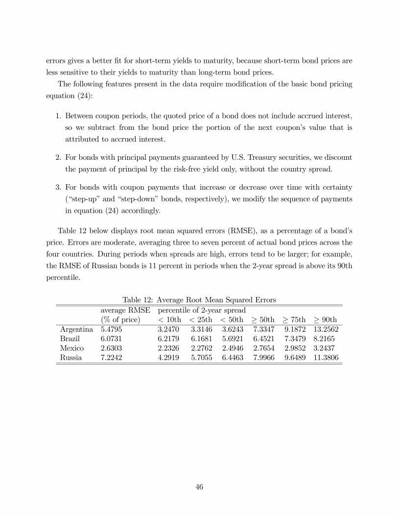
errors gives a better fit for short-term yields to maturity, because short-term bond prices are

less sensitive to their yields to maturity than long-term bond prices.

The following features present in the data require modification of the basic bond pricing

equation (24):

1. Between coupon periods, the quoted price of a bond does not include accrued interest,

so we subtract from the bond price the portion of the next coupon’s value that is

attributed to accrued interest.

2. For bonds with principal payments guaranteed by U.S. Treasury securities, we discount

the payment of principal by the risk-free yield only, without the country spread.

3. For bonds with coupon payments that increase or decrease over time with certainty

(“step-up” and “step-down” bonds, respectively), we modify the sequence of payments

in equation (24) accordingly.

Table 12 below displays root mean squared errors (RMSE), as a percentage of a bond’s

price. Errors are moderate, averaging three to seven percent of actual bond prices across the

four countries. During periods when spreads are high, errors tend to be larger; for example,

the RMSE of Russian bonds is 11 percent in periods when the 2-year spread is above its 90th

percentile.

Table 12: Average Root Mean Squared Errorsaverage RMSE percentile of 2-year spread(% of price) < 10th < 25th < 50th ≥ 50th ≥ 75th ≥ 90th

Argentina 5.4795 3.2470 3.3146 3.6243 7.3347 9.1872 13.2562Brazil 6.0731 6.2179 6.1681 5.6921 6.4521 7.3479 8.2165Mexico 2.6303 2.2326 2.2762 2.4946 2.7654 2.9852 3.2437Russia 7.2242 4.2919 5.7055 6.4463 7.9966 9.6489 11.3806

46

Further Statistics on Spread Curves

Tables 13 reports further spread curves and spread volatilities for all countries.

Table 13: Average Spreads and VolatilityMaturity Overall Std. Dev When 2-year spread is above/below nth percentile(years) (%) < 10th < 25th < 50th ≥ 50th ≥ 75th ≥ 90th

Argentina 2 4.77 6.26 1.10 1.60 2.10 7.44 11.03 19.645 5.27 3.83 1.97 2.60 3.24 7.31 9.52 14.5410 6.22 3.36 3.19 3.77 4.40 8.04 10.00 14.0615 6.63 3.30 3.70 4.25 4.87 8.39 10.31 14.12

Brazil 2 5.60 5.02 1.69 2.15 2.68 8.51 12.25 18.575 6.71 4.41 3.58 3.83 4.18 9.23 12.25 17.0710 7.14 2.93 4.79 5.25 5.35 8.93 10.84 13.3615 7.28 2.41 5.24 5.81 5.81 8.75 10.19 11.74

Mexico 2 1.84 1.36 0.42 0.62 0.94 2.74 3.49 4.845 2.46 0.97 1.57 1.74 2.01 2.90 3.32 4.4510 3.45 0.95 2.40 2.60 2.97 3.93 4.28 5.2715 3.87 0.98 2.72 2.93 3.35 4.40 4.74 5.66

Russia 2 4.44 2.65 1.70 2.03 2.62 6.25 7.88 9.875 5.37 2.59 2.86 3.10 3.52 7.22 9.03 10.5810 5.10 2.25 2.86 2.81 3.39 6.79 8.11 9.3615 4.92 2.21 2.80 2.62 3.28 6.54 7.62 8.76

47

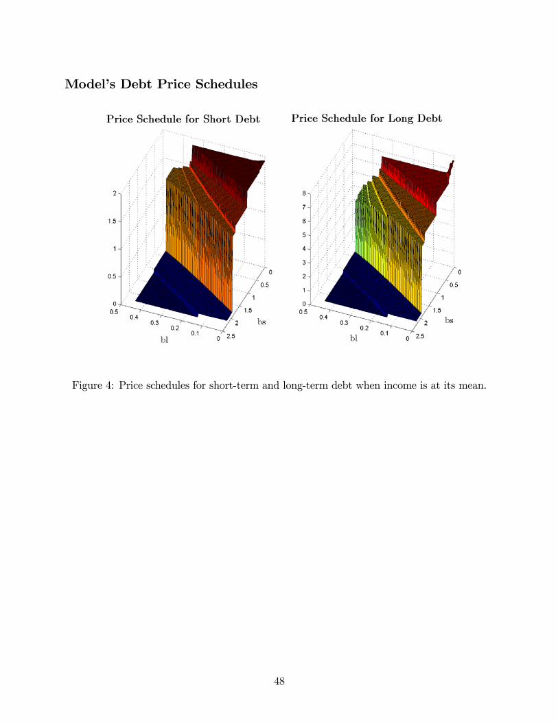
Model’s Debt Price Schedules

Figure 4: Price schedules for short-term and long-term debt when income is at its mean.

48