Embed Size (px)
Citation preview
Louisiana State UniversityLSU Digital Commons
LSU Doctoral Dissertations Graduate School
2015
Deepwater Gulf of Mexico Oil Spill ScenariosDevelopment and Their Associated RiskAssessmentMuhammad ZulqarnainLouisiana State University and Agricultural and Mechanical College, [email protected]
Follow this and additional works at: https://digitalcommons.lsu.edu/gradschool_dissertations
Part of the Petroleum Engineering Commons
This Dissertation is brought to you for free and open access by the Graduate School at LSU Digital Commons. It has been accepted for inclusion inLSU Doctoral Dissertations by an authorized graduate school editor of LSU Digital Commons. For more information, please [email protected].
Recommended CitationZulqarnain, Muhammad, "Deepwater Gulf of Mexico Oil Spill Scenarios Development and Their Associated Risk Assessment" (2015).LSU Doctoral Dissertations. 3452.https://digitalcommons.lsu.edu/gradschool_dissertations/3452
DEEPWATER GULF OF MEXICO OIL SPILL SCENARIOS DEVELOPMENT AND
THEIR ASSOCIATED RISK ASSESSMENT
A Dissertation
Submitted to the Graduate Faculty of the
Louisiana State University and
Agricultural and Mechanical College
in partial fulfillment of the
requirements for the degree of
Doctor of Philosophy
in
The Department of Petroleum Engineering
by
Muhammad Zulqarnain
B.S., Quaid-i-Azam University, 1999
M.S., Pakistan Institute of Engineering and Applied Sciences, 2001
M.S., Louisiana State University, 2012
August 2015
ii
ACKNOWLEDGEMENTS
I am deeply thankful to my advisor, Prof. Mayank Tyagi for his support, guidance and
encouragement throughout the course of this work. His valuable inputs were extremely helpful
during this research work and dissertation writing. He showed me many ways to approach a
problem and the need to be persistent in order to accomplish the tasks.
I am thankful to all of my committee members for their valuable time and feedback to
improve my research work. Thanks to Prof. Gerald. M. Knapp for his time and guidance in
learning and using some of the reliability engineering techniques and tools. Thanks to Prof.
Stephen O. Sears for his guidance in conducting the underground blow out scenario and
providing the relevant material. Special thanks to Prof. John R. Smith for his time to thoroughly
review this document and his feedback for improvements. Thanks to Prof. Juan M. Lorenzo and
Prof. Aly M. Aly for their valuable advice and recommendations to present the results in more
effective way.
Special thanks to Jason Mathews and his colleagues from Bureau of Safety and
Environmental Enforcement (BSEE) for providing very useful data, to perform the analysis.
Thanks to Ian Wright for providing LOGAN Fault and Event Tree analysis software for this
study.
I wish to express my gratitude to Shell Corporation for providing the financial support to
carry out this research work.
iii
TABLE OF CONTENTS
ACKNOWLEDGEMENTS ............................................................................................................ ii
LIST OF TABLES ........................................................................................................................ vii
LIST OF FIGURES ........................................................................................................................ x
NOMENCLATURE .................................................................................................................... xiv
ABSTRACT .................................................................................................................................... 1
INTRODUCTION .......................................................................................................................... 3
CHAPTER 1: OVERVIEW OF DEEPWATER OIL AND GAS OPERATIONS AND RISK
ASSESSMENT ............................................................................................................................... 5
1.1 Basic Constituents of a Spill Scenario ...................................................................... 5 1.2 Quantitative Risk Analysis ....................................................................................... 8
1.2.1 Environmental Damage ................................................................................... 10 1.3 Objectives of this Study .......................................................................................... 12 1.4 Well Barriers and Well Control .............................................................................. 13
1.4.1 Barrier in Normal Drilling Operations ............................................................. 13 1.4.2 Barriers during Normal Production Operations ............................................... 14
1.5 Scenarios Studied .................................................................................................... 14 1.5.1 Scenario-1: Drilling/Man-made/High potential ............................................... 15
1.5.2 Scenario-2: Drilling/Underground/Flow outside the well ............................... 16 1.5.3 Scenario-3: Production/Man Made/High Potential/ Sand Screen Failure ....... 16
1.5.4 Scenario-4: Production FPSO/Man Made/Nature............................................ 17 1.5.5 Scenario-5: Severe Weather/Loss of Position/Mudslide/Production Halt ....... 18
1.6 Fault Tree Analysis (FTA) ...................................................................................... 18
1.6.1 Algebraic gate operations with probabilities ................................................... 20 1.7 Reliability Analysis ................................................................................................. 21
1.8 Data Sources ........................................................................................................... 21
CHAPTER 2: FRAMEWORK FOR RISK ASSESSMENT PROCESS ..................................... 24
2.1 Representative Well Location ................................................................................. 25 2.2 GoM Geology ......................................................................................................... 25 2.3 Representative reservoir properties ........................................................................ 26
2.3.1 Reservoir Pressure ........................................................................................... 27 2.3.2 Reservoir Temperature ..................................................................................... 27 2.3.3 Porosity and Permeability Trends .................................................................... 28
2.4 Reservoir Properties with Lognormal Distribution ................................................ 29
2.5 Selected Well Schematics ....................................................................................... 30 2.6 Fluid Flow Simulation Setup .................................................................................. 31
iv
CHAPTER 3: OIL SPILL RISK ASSESSMENT OF A DEEPWATER EXPLORATORY
DRILLING WELL (SCENARIO-1)............................................................................................. 35
3.2 Introduction ............................................................................................................. 36 3.2.1 Description of Capping and Containment System ........................................... 37 3.2.2 Well Barriers .................................................................................................... 38 3.2.3 Methodology .................................................................................................... 39 3.2.4 Representative Well, Reservoir Properties, and QRA Procedure .................... 39
3.3 Historical Trends in the GoM ................................................................................. 41 3.3.1 Kick causes and Frequency .............................................................................. 41 3.3.2 Blowout Frequency .......................................................................................... 42 3.3.3 Blowout Duration ............................................................................................. 43 3.3.4 Reservoir Penetration and Kick Occurrences .................................................. 44
3.3.5 Flow Path Distribution and Restrictions to Flow ............................................. 45 3.3.6 Flow Rate, Spill Duration and Fault Tree Analysis ......................................... 46
3.4 Results ..................................................................................................................... 47 3.4.1 Blowout Frequency/Probability Calculation .................................................... 47 3.4.2 Fussell Vesely Importance Measure ................................................................ 49 3.4.3 WCD Subsea Release Calculations for P50 Values......................................... 50 3.4.4 Implications for Environmental Damage Assessment ..................................... 53 3.4.5 Construction of Risk Matrix ............................................................................ 55
3.5 Concluding Remarks on Risk Associated With Deepwater Exploratory Well ...... 56
CHAPTER 4: RISK ASSESSMENT OF A DEEPWATER GULF OF MEXICO
UNDERGROUND BLOWOUT (SCENARIO-2) ........................................................................ 59 4.1 Natural Hydrocarbon Seeps in GoM ...................................................................... 60
4.1.1 Geological Features ......................................................................................... 60 4.1.2 Popeye-Genesis Minibasin ............................................................................... 60 4.1.3 Auger Basin ..................................................................................................... 61 4.1.4 Well stability concerns before Macondo shut in during blowout .................... 62
4.2 Crater/Subsidence Hazard ....................................................................................... 63 4.2.1 Conditions for Vertical Subsidence ................................................................. 65
4.3 Faults Barriers or Migratory Paths.......................................................................... 65 4.3.1 Cap Rock Failure ............................................................................................. 66
4.3.2 Fault Permeability and Thickness .................................................................... 68 4.4 Reservoir Simulation Setup Flow through Faulted Zone ....................................... 71 4.5 Simulation Results flow through Faulted Zone ...................................................... 74 4.6 Observations & Conclusions .................................................................................. 77
CHAPTER 5: OIL SPILL RISK ASSESSMENT OF A SAND CONTROL ELEMENT
FAILURE LEADING TO BLOWOUT DURING NORMAL PRODUCTION OPERATIONS
(SCENARIO-3)............................................................................................................................. 78
5.1 Introduction ............................................................................................................. 79 5.2 Literature Survey .................................................................................................... 80 5.3 Methodology ........................................................................................................... 81
v
5.4 Primary Well Barrier Failure Analysis ................................................................... 82
5.5 Secondary Well Barrier Failure Analysis ............................................................... 84 5.6 Analysis Setup ........................................................................................................ 87 5.7 Results and Discussion ........................................................................................... 87
5.7.1 Fault Tree Analysis .......................................................................................... 87 5.7.2 Fussell Vesely Importance (FVI) Measure ...................................................... 89 5.7.3 Blowout Uncertainty Analysis ......................................................................... 90 5.7.4 Flow Rate Calculations .................................................................................... 91 5.7.5 Environmental Risk Assessment ...................................................................... 91
5.8 Concluding Remarks for Scenario-3 ....................................................................... 94
CHAPTER 6: A REVIEW OF OIL SPILL RISK ASSOCIATED WITH FPSO DEPLOYMENT
IN GOM (SCENARIO-4) ............................................................................................................. 96
6.1 Typical FPSO Configuration for GoM ................................................................... 97 6.2 Station Keeping ....................................................................................................... 99
6.2.1 Mooring Configurations ................................................................................. 100
6.2.2 FPSO Roll motion effect on Mooring ............................................................ 101 6.2.3 FPSO Yawing Motion .................................................................................... 101
6.3 Fuel Offloading Operations .................................................................................. 101 6.4 Shuttle Tanker Collision Analysis ........................................................................ 102
6.4.1 FPSO Tandem Offloading Analysis .............................................................. 104
6.5 All Accidents Involving FPSO UKCS 1980-2005 ............................................... 107 6.6 Other FPSO Areas of Concern Identified by Researchers .................................... 108
6.7 Risk Matrix ........................................................................................................... 109 6.8 FPSO Observations and Conclusions ................................................................... 109
CHAPTER 7: OIL SPILL RISK ASSOCIATED WITH SEVERE WEATHER CONDITIONS
IN THE GULF OF MEXICO (SCENARIO-5) .......................................................................... 111
7.1 Hurricane Categories and Their Occurrences in the GoM.................................... 111 7.2 Mudslide Slide Hazard in Mississippi Current Delta ........................................... 113
7.2.1 Installation Damage and Oil Spill due to Mud Slide ..................................... 114
7.3 Metocean Data ...................................................................................................... 116 7.4 Weather Induced Adrift Of Offshore Dynamic Structures ................................... 117
7.5 Pipeline Damage Due to High Wind Loads .......................................................... 120 7.5.1 Pipelines Damaged Types and Related Spills ................................................ 121
7.6 Platform Damages Due To High Wind Loads ...................................................... 122 7.6.1 Damage Categories ........................................................................................ 123 7.6.2 Platform related Oil spill ................................................................................ 124
7.7 Mudslide Hazard Calculation ............................................................................... 124
7.7.1 Example: Mudslide Risk Assessment for SP-70 Block ................................. 127 7.7.2 Spill volume calculations: mudslide resulting in pipeline damage ................ 128 7.7.3 Spill volume calculations: mudslide resulting in riser damage...................... 130
7.8 Mudslide resulting in severely damaging a production platform ......................... 130 7.8.1 Modeling of Mudslide Risk ........................................................................... 132
7.9 Production Halt ..................................................................................................... 133
vi
7.10 Spill Response Technologies for weather induced Spill .................................... 134
7.11 Qualitative Risk Matrix ...................................................................................... 135 7.12 Conclusions and Observations ............................................................................ 136
CHAPTER 8: CONCLUDING REMARKS AND FUTURE DIRECTIONS ........................... 140
8.1 Scenario-1: Exploratory Well ............................................................................... 140 8.2 Scenario-2: Underground Blowout ....................................................................... 142 8.3 Scenario-3: Production Well ................................................................................. 143 8.4 Scenario-4: FPSO ................................................................................................. 144 8.5 Scenario-5: Weather Induced Spills ..................................................................... 145
8.6 Approximations and Limitations .......................................................................... 147 8.7 Future Directions .................................................................................................. 148
REFERENCES ........................................................................................................................... 150
APPENDIX-A: PALEOGENE WELL SCHEMATIC AND WORST CASE DISCHARGE
RATES ........................................................................................................................................ 158
APPENDIX-B: HISTORICAL SPILLS (INCLUDING ALL) AND THEIR CAUSES IN GOM
..................................................................................................................................................... 160
VITA ........................................................................................................................................... 162
vii
LIST OF TABLES
Table 1: Standard symbols used in the fault tree analysis ............................................................ 19
Table 2: Some of the blowout and reliability data sources and their availability ......................... 22
Table 3: Some of the data sources for equipment leaks, vessel collision, falling objects and
transportation accidents. Detailed references can be found in the additional references section . 23
Table 4: Typical required input parameters for estimation of worst case discharge rates for
drilling and production scenario ................................................................................................... 24
Table 5: Reservoir properties obtained by fitting lognormal distribution and using Monte Carlo
simulation ...................................................................................................................................... 29
Table 6: The casing program for the selected deepwater Neogene well (Fontenot, 2013) .......... 31
Table 7: Black oil properties ......................................................................................................... 31
Table 8: Reservoir properties for one of the representative GoM deepwater sand (based on data
from RPSEA, 2010) ...................................................................................................................... 41
Table 9: Deepwater GoM kick data with its causes (Holand, 2007) ............................................ 41
Table 10: Well drilled and number of kicks for the exploratory drilling in the GoM deepwaters
(Holand, 2007) .............................................................................................................................. 42
Table 11: Blowout probability during exploratory and development drilling in deepwaters of
world except North Sea, data mostly consists of GoM (OGP- No. 434-2, 2010) ........................ 43
Table 12: Blowout duration for deepwater wells when capping and relief well are the only option
considered ..................................................................................................................................... 44
Table 13: Relation between reservoir penetration and kick occurrence (Oljeindustriens, 2010) . 45
Table 14: Historical trends for hydrocarbon release (Oljeindustriens, 2010 & Smith, 2012) ...... 45
Table 15: Importance analysis showing the contribution of some of the most influencing basic
events with the unexpected pore pressure is the main contributor ............................................... 49
Table 16: Subsea release flow path probability and rates corresponding to P50 value
(RPP:Release Point Probability,FPP:Flow Path Probability, PD:Penetration Depth,
PDP:Penetration Depth Probability, FSP:Functional State Probability, PPB:Probability Per
Blowout) ....................................................................................................................................... 51
Table 17: Risk table categorized for functional BOP state during blowout with only relief well
option (PPB:Probability Per Blowout, PPDW: Probability Per Drilled Well) ............................. 53
viii
Table 18: Calculated value of fault permeability and thickness ................................................... 68
Table 19: Reservoir properties of shallower low pressure and deeper high pressure zone .......... 72
Table 20: Underground blowout cases study flow through a fault ............................................... 72
Table 21: Leak off test data for Popeye Field [From Seldon, 2005] ............................................ 73
Table 22: Sand control failure from King et al. (2003) ............................................................... 82
Table 23: Primary barrier failure rates .......................................................................................... 83
Table 24: Secondary barrier failure rates ...................................................................................... 84
Table 25: Blowout probability during normal production operations OGP (2010)...................... 85
Table 26: Blowout duration probability distribution adopted from ACONA (2012) ................... 85
Table 27: Fussell Vesely importance analysis results................................................................... 89
Table 28: Subsea release paths and rates, SST: Subsurface Release through Tubing, SSA: Subsea
Release through Annulus, FSP: Flow Restriction Probability, PPB: Probability Per Blowout .... 91
Table 29: Impact Factor Calculation for Base and Modified Cases ............................................. 92
Table 30: FPSO configuration for GOM deployment from (Regg et al., 2000) ........................... 98
Table 31: Reported incidents during tandem transfer in offshore UK (Chen-2003) .................. 105
Table 32: Oil tanker oil spill frequencies (From OGP-Report No. 434-10, 2010) ..................... 105
Table 33: Estimation of GoM shuttle tanker arrivals per year .................................................... 106
Table 34: Shuttle tanker related incidents with approximate arrivals for the typical FPSO
considered for GoM and different shuttle tanker capacities ....................................................... 106
Table 35: FPSO Incident data UKCS for period of 1980-2005 reported in (HSE - RR567) ..... 107
Table 36: Storm classification using Saffir-Simpson Scale ........................................................ 112
Table 37: Hurricane condition data for central GoM region (From API 2INT-MET, 2007) ..... 117
Table 38: MODUs Jack-Up drifting from their original location (From Sharples, 2009) .......... 119
Table 39: Pipeline damages reports for different hurricanes, NR* stands for not reported ....... 120
Table 40: Oil spilled due to Hurricanes Katrina & Rita (DNV Report NO. 448 14183) ........... 122
ix
Table 41: Platform exposed, damaged or destroyed during past hurricanes (From DNV Report-
44814183) ................................................................................................................................... 122
Table 42: Oil spilled due to destruction or damages to offshore structures ................................ 124
Table 43: Parameters specific to South Pass Block 70 (From Nodine et al., 2007) ................... 127
Table 44: Safety factor calculations for South Pass block 70 in the Gulf of Mexico ................. 128
Table 45: Amount of oil spilled due to mudslide slide resulting in pipeline rupture ................. 129
Table 46: Platform spill as a result of riser leaks due to high wind and high wave generated
stresses ........................................................................................................................................ 130
Table 47: Platform spill for a production platform in the shallow water GoM .......................... 132
Table 48: Production Shut-In due to hurricane, historic trends [data taken from DNV REPORT
NO. 448 14183, 2007] ................................................................................................................ 134
Table 49: Paleogene period deepwater well (Alaminos Canyon) subsea release rates and
probabilities for P50 values of reservoir properties .................................................................... 159
Table 50: Historical GoM and PAC Pipeline Spill and their Causes (1972-2010) [Table is taken
from (Bercha, 2013)] .................................................................................................................. 160
Table 51: GoM and PAC OCS Platform Hydrocarbon Spill Statistics (1977-2010) [Table is taken
from (Bercha, 2013] .................................................................................................................... 161
x
LIST OF FIGURES
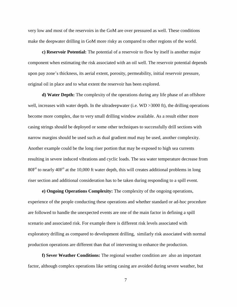
Figure 1: Life phases of an offshore oil & gas well ........................................................................ 6
Figure 2: Schematic showing the necessary steps in risk estimation .............................................. 9
Figure 3: Kick leading to a blowout during exploratory drilling .................................................. 15
Figure 4: Event tree of an underground blowout .......................................................................... 16
Figure 5: Sand control element failure leading to a blowout for a producing well, the expansion
of only the production packer branch is shown ............................................................................ 17
Figure 6: Differences between FPSO and other type of production platforms............................. 18
Figure 7: Map showing GOM blocks with two selected representative well locations................ 25
Figure 8: (a) Reservoir pressure variation for Paleogene period Wilcox sand in the GoM (joshua
oletu etal. 2013), (b) pressure variation with depth in the gulf of Mexico with geological time
scale (haeberle, 2005) ................................................................................................................... 27
Figure 9: (a) Reservoir temperature variation for Paleogene period Wilcox sand in the GoM
(Joshua Oletu etal. 2013), (b) temperature variation with geological time scale (Haeberle, 2005)
....................................................................................................................................................... 28
Figure 10: Well schematic (a) deepwater well: Neogene GoM (Fontenot, 2013), (b)
Ultradeepwater well: Paleogene ................................................................................................... 30
Figure 11: Partial penetration into a reservoir
(http://petrowiki.org/Fluid_flow_with_formation_damage) ........................................................ 33
Figure 12: Capping and Containment system of Marine Well Containment Company (MWCC,
2011) ............................................................................................................................................. 38
Figure 13: Primary and secondary barriers in a drilling well (NORSOK Standard, 2013) .......... 39
Figure 14: Results of Monte Carlo simulation and fitted log-normal and triangular distribution 40
Figure 15: Blowout uncertainty analysis for 100,000 trials of Monte Carlo simulations with a
slightly skewed normal distribution having a peak frequency of 2.9 ×10⁻³
.................................. 47
Figure 16: Fault tree analysis of a deepwater exploratory drilling well ....................................... 48
Figure 17: Pressure decline and flow rate variations with time .................................................... 52
xi
Figure 18: Risk matrix for the deepwater GoM exploratory drilling well .................................... 55
Figure 19: Underground blowout and its consequences ............................................................... 59
Figure 20: An example seismic map in northern GoM slope with source and migration pathways
(From Hood et al., 2002)............................................................................................................... 61
Figure 21: Rupture disk location in Macondo well (From Hickman et al. (2011) ....................... 63
Figure 22: Pressure and Stresses in the Popeye-Genesis minibasin based on leak off test data
[From Seldon, (2005)] .................................................................................................................. 66
Figure 23: Stress and strain curves for original and re-sheared sandstones [From Dewhurst, 2002]
....................................................................................................................................................... 67
Figure 24: Reservoir simulation model, showing the two interconnecting zones and conductive
fault used for studying Underground Blowout ............................................................................. 73
Figure 25: Pressure change propagation after 100 years of flow from high pressure to lower
pressure shallower zone ................................................................................................................ 74
Figure 26: Pressure change propagation after 100 years of flow from high pressure to lower
pressure shallower zone ................................................................................................................ 75
Figure 27: Pressure contour of the deeper and shallower zone and the pressure change with time
....................................................................................................................................................... 75
Figure 28: Pressure contour of the deeper and shallower zone and the pressure change with time
....................................................................................................................................................... 76
Figure 29: Shallower zones pressure variations with time for Case- 5. Fracture
dilation/propagation conditions are met in 3 years’ time frame ................................................... 76
Figure 30: Schematic of a horizontal subsea tree (From NORSOK standard D-010, 2013) ........ 80
Figure 31: Major tubing failure causes and their contribution King et al. (2010) ........................ 83
Figure 32: Possible flow paths [From Petersen (2011)] ............................................................... 86
Figure 33: Production fault tree analysis setup ............................................................................. 88
Figure 34: Blowout uncertainty with a nearly normal distribution ............................................... 90
Figure 35: Comparison of all three cases through risk matrix ...................................................... 93
Figure 36: FPSO in operation (From http://www.bluewater.com/wp-
content/uploads/2013/03/4.2.3-Subsea-Field-Layout.jpg)............................................................ 97
xii
Figure 37: (a) Spread mooring and (b) Single point turret mooring [Reference: energyclaims
http://www.energyclaims.net/assets/FPSO-Presentation.pdf) .................................................... 100
Figure 38: (a) Tandem and (b) side by side offloading from FPSO (From Regg-2000) ............ 102
Figure 39: FPSO related incident categorization dada taken from Smith (2003). ...................... 108
Figure 40: Risk matrix for spills related to FPSO Operations .................................................... 109
Figure 41: Historical storm paths in the GoM (From Hitchcock et al., 2006) ............................ 112
Figure 42: Mud sensitive area in the Mississippi Delta (Hitchcock et al., 2006) ....................... 113
Figure 43: Return period of mudslides and corresponding pipelines in that region [From Nodine
et al., 2007) ................................................................................................................................. 114
Figure 44: Pipeline and platform damage resulting in oil spills ................................................. 115
Figure 45: Location of Taylor platform and oil sheen visible at surface [From RRT-6] ........... 115
Figure 46: Division for Metocean conditions and region classification (From API RP 2INT-MET
2007). .......................................................................................................................................... 116
Figure 47: An example of spread mooring [From API-RP 2SK] ............................................... 117
Figure 48: Map of rig locations and paths adrift after hurricane Rita (From DNV Report NO. 448
14183) ......................................................................................................................................... 118
Figure 49: Pipeline damage reported for Hurricanes Katrina and Rita [From DNV Report-
44814183] ................................................................................................................................... 120
Figure 50: Pipeline damages by its location (DNV Report NO. 448 14183) ............................. 121
Figure 51: Reported failure category distribution (From DNV Report- 44814183) .................. 123
Figure 52: Chevron’s Typhoon TLP - pre and post hurricane Rita condition (From DNV Report-
44814183) ................................................................................................................................... 123
Figure 53: Stability chart based on limit equilibrium stability model to find the value of safety
factor (From Nodine et al., 2007) ............................................................................................... 126
Figure 54: Approximate location of South Pass Block 70 shown by red circle (taken from
Offshore Mag) ............................................................................................................................. 127
Figure 55: Schematic of trunk line from leaking point to terminal ............................................ 129
Figure 56: Selected well schematic, regional reservoir properties and the selected values used are
shown. ......................................................................................................................................... 131
xiii
Figure 57: Cone shaped collector used in oil suction on Taylor Energy’s buried platform (from
RRT-6) ........................................................................................................................................ 135
Figure 58: Qualitatively risk matrix for spills due to severe weather conditions ....................... 136
Figure 59: A qualitative presentation of risk assessment steps to be adopted for offshore
structures due to adverse weather conditions .............................................................................. 139
Figure 60: Well Schematic of the ultradeepwater Paleogene well ............................................. 158
xiv
NOMENCLATURE
ASV Annular Safety Valve
BC Base Case
Bo Oil Formation Volume Factor
BOPD Barrels of Oil per Day
GoM Gulf of Mexico
GOR Gas Oil Ratio
HPHT High Pressure High Temperature
K Permeability (mD)
MC Modified Case
MIC Modified Improved Case
MMbbl Million Barrels
P10 P10 refers to a p-value of 0.9
P90 P90 refers to a p-value of 0.1
Pb Bubble Point Pressure
PI Productivity Index
PR Reservoir Pressure
QRA Quantitative Risk Assessment
SCSSV Surface Controlled Subsurface Safety Valve
UBO Underground Blow Out
WCD Worst Case Discharge rate
1
ABSTRACT
World’s growing energy demand has pushed oil companies to explore and produce
hydrocarbons in complex and technologically challenging deepwater environments. These
difficult and complex operations involve the risk of major accidents as well, demonstrated by
disasters such as the explosion and fire on the UK production platform Piper Alpha and
capsizing of the Deepwater Horizon rig in the Gulf of Mexico (GoM). Accidents cause death,
suffering, pollution of the environment, disruption of business and bad reputation to oil industry.
A quantitative risk analysis technique has been used in this study to identify and
categorize risk associated with different life phases of a deepwater well. Volume of oil released
to the environment is used as a risk indicator. Five oil spill scenarios related to drilling and
production life phases of a deepwater well are modeled.
Risks associated with drilling an exploratory well in the deepwaters of GoM are analyzed
in Scenario-1. A representative well location and corresponding reservoir properties were used to
estimate the worst case discharge rates (WCD). Fault tree analysis (FTA) was performed to
identify and categorize different hazards. Unexpected pore pressure and delayed response to an
emergency situation were identified as two most important parameters contributing to overall
risk of the system.
In Scenario-2 an underground blowout was modeled by using representative geological
settings from Popeye-Genesis field. A shallower low pressure zone is exposed to a deeper high
pressure zone during drilling. The time to recharge the shallower zone to its fracture pressure is
estimated. The shallower zone will transmit hydrocarbons to sea floor once its fracture pressure
is reached. Risks associated with production life phase of a deepwater well are modeled in
2
scenario-3. A representative well location and corresponding reservoir properties were used to
estimate the WCD. FTA showed that sand screen and subsea tree control failures were main
elements contributing to risk.
In scenario-4 risk associated with floating production and offloading (FPSO) system for
GoM are quantitatively and qualitatively presented. Scenario-5 deals with oil spill risk associated
with severe weather conditions. An example mudslide calculation for SP-70 block of GoM is
presented.
3
INTRODUCTION
This section briefly introduces each chapter of the dissertation.
Chapter one covers, basic elements of a spill scenario, introduction of techniques used for
Quantitative Risk Assessment (QRA), oil and gas well barriers and their importance, and some
of the data sources that can be used to conduct QRA of offshore operations.
Second chapter deals with solution methodology adopted to perform the quantitative risk
assessment. Selection of representative well, reservoir properties and fluid flow models are
discussed in detail.
In chapter 3 quantitative risk assessment of a deepwater exploratory oil well is presented
and is referred as Scenario-1. A representative well from the Mississippi canyon in the Gulf of
Mexico is studied for potential worst cases discharge (WCD) rates. Oil spill duration is estimated
from historical spill durations and success of different spill response techniques. Product of
WCD rate and duration gives the most probable oil spill amount. Blowout frequency is computed
using fault tree analysis. Through sensitivity/importance analysis risk prone areas have been
identified. The effectiveness of newly built response systems, called capping and containment
systems is also analyzed in reducing the risk of large oil spills.
Risks associated with the underground blowout (Scenario-2) are addressed in Chapter 4.
It is assumed that during drilling a high pressure reservoir is accidently exposed to a low pressure
shallower zone. A conducting fault or a highly permeable zone connects these zones. A
representative reservoir’s settings from Popeye-Genesis filed in the deepwater GoM is selected
to model this scenario. It is assumed that the shallower zone’s cap rock sealing capacity is lost
when its pressure is reached to its leakoff test value. Then the set of exiting or induced fractures
4
or faults in the cap rock transmits the hydrocarbons to the sea floor. Under these assumptions the
charging time for the shallower zone to reach its leak off test value is estimated by conducting
reservoir simulations. A parametric study is conducted by changing the shallower zone’s volume
and connecting zone’s permeability and recharging time for shallower zone is estimated.
In chapter 5, quantitative oil spill risk assessment of a production well (Scenario-3) is
performed. It is hypothesized that a sand screen failure leads to a blowout. Representative well
location, well barriers and reservoir properties in the GoM are selected to compute worst case
discharge rates and blowout frequency. Spill duration is estimated based on the historic spill data
and the effectiveness of various spill response techniques. Sensitivity/importance analysis is
conducted using fault tree analysis and most sensitive areas are identified.
In chapter 6 risk associated with FPSO (Scenario-4) are quantitatively and qualitatively
studied. FPSO is different from other production platforms due to its large storage capacity,
station keeping requirements and shuttle tanker offloading. A proposed FPSO configuration for
GoM is studied to estimate amount of spill during shuttle tanker transportations and fuel
offloadings.
Weather induced oil spill risks are analyzed in chapter 7 (Scenario-5). Severe weather can
induce, mudslide, damage/destroy platforms and adrift of offshore floating structures. An
example oil spill volume calculation due to mudslide damage in SP-70 block of GoM is
presented for platform damage, production riser’s damage and rupture of large oil carrying
pipeline.
Chapter 8 summarizes the conclusion of all of the five modeled oil spill scenarios.
5
CHAPTER 1: OVERVIEW OF DEEPWATER OIL AND GAS OPERATIONS AND
RISK ASSESSMENT
Offshore oil and gas exploration and production operations, involve the use of some of
the cutting edge and challenging technologies of the modern time. These technological complex
operations involves the risk of major accidents as well, which have been demonstrated by
disasters such as the explosion and fire on the UK production platform piper alpha, the Canadian
semi-submersible drilling rig Ocean Ranger and the explosion and capsizing of Deepwater
horizon rig in the Gulf of Mexico. Offshore production may be one of the major sources of
revenue for some of the companies and countries.
Major accidents like Macondo represent the ultimate, most disastrous way in which
an offshore engineering project can end up. Accidents cause death, suffering, pollution of
the environment and disruption of businesses. They attract attention from the news media
and linger in the public memory for a long time, causing concern about safety of offshore
oil and gas production operations. People may start questioning about the safety of offshore
operations. In order to address these concerns and show that a balance between the interests of
safety and the economics of oil and gas production can be achieved, a technique called
Quantitative Risk Assessment (QRA) can be used. By conducting QRA, risk and their
significance for the entire life phase of an offshore project can be quantitatively estimated. It will
help in identifying the safety-critical procedures and equipment. QRA may also be used to show
the project’s acceptability to regulators and workforce.
1.1 Basic Constituents of a Spill Scenario
The probability of occurrence of an oil spill and its consequences are a combination of
the following factors, well’s life phase, geological features, reservoir potential, operational
6
complexities, water depths, type of installations and severe weather conditions. These are briefly
described below.
a) Well Life Phase: The life phase of a well is very important factor in describing the
spill scenario. There are different risks associated with different life phases of a well. Operational
conditions and the reservoir’s potential to flow varies with well’s life phase which result in
different hazards with each life phase of an offshore well. For example, there are more risks
associated with drilling an exploratory well as compared to drilling a development well. These
risks are due to uncertainties in the geology and reservoir being at its full potential at the time of
exploratory well. An offshore well’s life span can be divided into three broad categories of
drilling, production and abandonment phase. These are briefly described below.
1- Drilling can be subdivided into exploratory and development drilling.
2- Production can be subdivided into normal production operations and intervention
3- Temporary Abandonment and Permanent Abandonment
These are shown in Figure 1.
Figure 1: Life phases of an offshore oil & gas well
b) Geological Complexities: In GoM usually the operational window during drilling
phase is very narrow, i.e. the difference between pore pressure and formation fracture pressure is
7
very low and most of the reservoirs in the GoM are over pressured as well. These conditions
make the deepwater drilling in GoM more risky as compared to other regions of the world.
c) Reservoir Potential: The potential of a reservoir to flow by itself is another major
component when estimating the risk associated with an oil well. The reservoir potential depends
upon pay zone’s thickness, its aerial extent, porosity, permeability, initial reservoir pressure,
original oil in place and to what extent the reservoir has been explored.
d) Water Depth: The complexity of the operations during any life phase of an offshore
well, increases with water depth. In the ultradeepwater (i.e. WD >3000 ft), the drilling operations
become more complex, due to very small drilling window available. As a result either more
casing strings should be deployed or some other techniques to successfully drill sections with
narrow margins should be used such as dual gradient mud may be used, another complexity.
Another example could be the long riser portion that may be exposed to high sea currents
resulting in severe induced vibrations and cyclic loads. The sea water temperature decrease from
80Fo to nearly 40F
o at the 10,000 ft water depth, this will creates additional problems in long
riser section and additional consideration has to be taken during responding to a spill event.
e) Ongoing Operations Complexity: The complexity of the ongoing operations,
experience of the people conducting these operations and whether standard or ad-hoc procedure
are followed to handle the unexpected events are one of the main factor in defining a spill
scenario and associated risk. For example there is different risk levels associated with
exploratory drilling as compared to development drilling, similarly risk associated with normal
production operations are different than that of intervening to enhance the production.
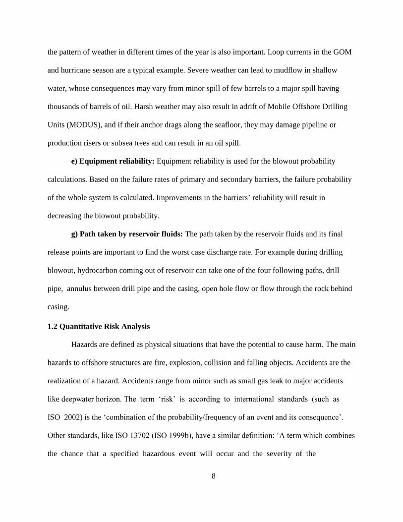
f) Sever Weather Conditions: The regional weather condition are also an important
factor, although complex operations like setting casing are avoided during severe weather, but
8
the pattern of weather in different times of the year is also important. Loop currents in the GOM
and hurricane season are a typical example. Severe weather can lead to mudflow in shallow
water, whose consequences may vary from minor spill of few barrels to a major spill having
thousands of barrels of oil. Harsh weather may also result in adrift of Mobile Offshore Drilling
Units (MODUS), and if their anchor drags along the seafloor, they may damage pipeline or
production risers or subsea trees and can result in an oil spill.
e) Equipment reliability: Equipment reliability is used for the blowout probability
calculations. Based on the failure rates of primary and secondary barriers, the failure probability
of the whole system is calculated. Improvements in the barriers’ reliability will result in
decreasing the blowout probability.
g) Path taken by reservoir fluids: The path taken by the reservoir fluids and its final
release points are important to find the worst case discharge rate. For example during drilling
blowout, hydrocarbon coming out of reservoir can take one of the four following paths, drill
pipe, annulus between drill pipe and the casing, open hole flow or flow through the rock behind
casing.
1.2 Quantitative Risk Analysis
Hazards are defined as physical situations that have the potential to cause harm. The main
hazards to offshore structures are fire, explosion, collision and falling objects. Accidents are the
realization of a hazard. Accidents range from minor such as small gas leak to major accidents
like deepwater horizon. The term ‘risk’ is according to international standards (such as
ISO 2002) is the ‘combination of the probability/frequency of an event and its consequence’.
Other standards, like ISO 13702 (ISO 1999b), have a similar definition: ‘A term which combines
the chance that a specified hazardous event will occur and the severity of the
9
consequences of the event’ (Vinnem, 2007). The likelihood of an event may be expressed either
as a frequency (i.e. the rate of events per unit time) or a probability (i.e. the chance of the event
occurring in specified circumstances). The consequence is the degree of harm caused by the
event (John Spouge, 1999). ‘QRA’ is used as the abbreviation for ‘Quantified Risk Assessment’
or ‘Quantitative Risk Analysis’. Quantitative risk assessment (QRA) is a means of making a
systematic analysis of the risks from hazardous activities, and forming a rational evaluation of
their significance, in order to provide input to a decision-making process (Spouge, 1999)
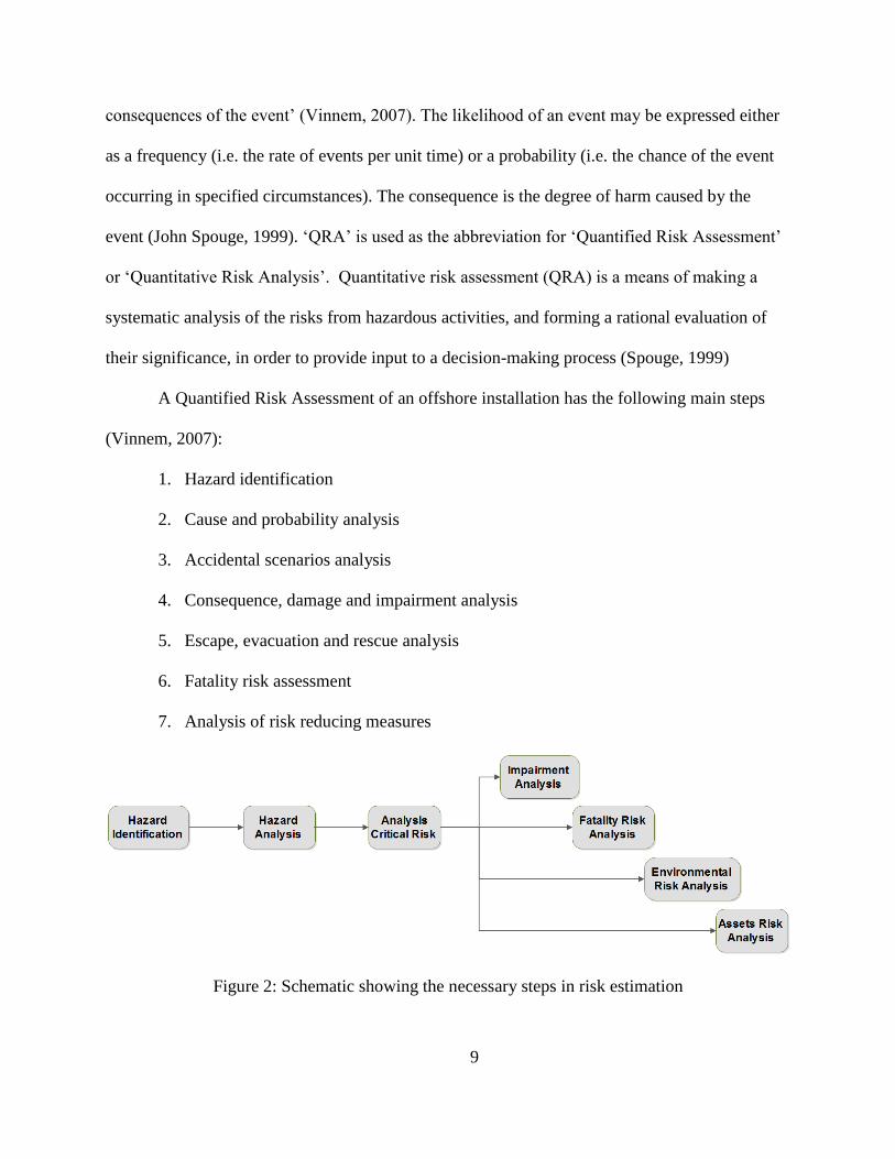
A Quantified Risk Assessment of an offshore installation has the following main steps
(Vinnem, 2007):
1. Hazard identification
2. Cause and probability analysis
3. Accidental scenarios analysis
4. Consequence, damage and impairment analysis
5. Escape, evacuation and rescue analysis
6. Fatality risk assessment
7. Analysis of risk reducing measures
Figure 2: Schematic showing the necessary steps in risk estimation
10
The consequences of an incident may be related to personnel, environment, assets and
production capacity. These are sometimes called ‘dimensions of risk’ (Vinnem, 2007). Only
environmental damages are addressed in this study.
1.2.1 Environmental Damage
Environmental damages due to spills are mostly dominated by the large infrequent spills
from blowouts, pipeline leaks, storage leaks, transportation leaks and accident involving shuttle
tankers. Small frequent process leak in the processing units, usually have low consequences as
they do not cause extensive environmental damage. In this study environmental damage is
categorized in terms of oil volume spilled to the sea, while the environmental risk is a
combination of oil volume released its proximity to shore lines, its decay in reaching the shore
lines and the sensitivity of the shore lines to oil spill. For the same volume of spilled oil, areas
rich in fisheries and tourism will have greater environmental risk as compared to areas that are
not abundant in fisheries and are not tourist’s destinations.
The quantified risk to the environment is a combination of:
Approximate amount of oil discharged to the environment.
Frequency of events with similar consequences for the environment.
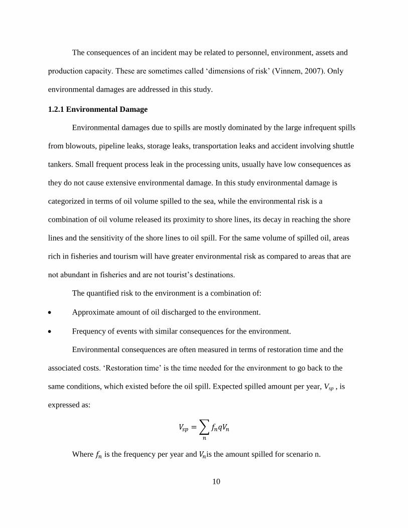
Environmental consequences are often measured in terms of restoration time and the
associated costs. ‘Restoration time’ is the time needed for the environment to go back to the
same conditions, which existed before the oil spill. Expected spilled amount per year, Vsp , is
expressed as:
𝑉𝑠𝑝 = ∑ 𝑓𝑛𝑞𝑉𝑛
𝑛
Where 𝑓𝑛 is the frequency per year and 𝑉𝑛is the amount spilled for scenario n.
11
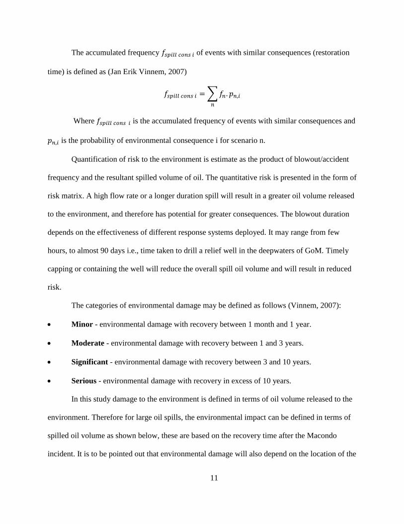
The accumulated frequency 𝑓𝑠𝑝𝑖𝑙𝑙 𝑐𝑜𝑛𝑠 𝑖 of events with similar consequences (restoration
time) is defined as (Jan Erik Vinnem, 2007)
𝑓𝑠𝑝𝑖𝑙𝑙 𝑐𝑜𝑛𝑠 𝑖 = ∑ 𝑓𝑛. 𝑝𝑛,𝑖
𝑛
Where 𝑓𝑠𝑝𝑖𝑙𝑙 𝑐𝑜𝑛𝑠 𝑖 is the accumulated frequency of events with similar consequences and
𝑝𝑛,𝑖 is the probability of environmental consequence i for scenario n.
Quantification of risk to the environment is estimate as the product of blowout/accident
frequency and the resultant spilled volume of oil. The quantitative risk is presented in the form of
risk matrix. A high flow rate or a longer duration spill will result in a greater oil volume released
to the environment, and therefore has potential for greater consequences. The blowout duration
depends on the effectiveness of different response systems deployed. It may range from few
hours, to almost 90 days i.e., time taken to drill a relief well in the deepwaters of GoM. Timely
capping or containing the well will reduce the overall spill oil volume and will result in reduced
risk.
The categories of environmental damage may be defined as follows (Vinnem, 2007):
Minor - environmental damage with recovery between 1 month and 1 year.
Moderate - environmental damage with recovery between 1 and 3 years.
Significant - environmental damage with recovery between 3 and 10 years.
Serious - environmental damage with recovery in excess of 10 years.
In this study damage to the environment is defined in terms of oil volume released to the
environment. Therefore for large oil spills, the environmental impact can be defined in terms of
spilled oil volume as shown below, these are based on the recovery time after the Macondo
incident. It is to be pointed out that environmental damage will also depend on the location of the
12
blowout, its proximity to the environmental sensitive areas alongside the spilled oil volume.
Keeping in view of the restoration time for Macondo incident, following approximated ranges
are defined
Minor: Impact = 1, Spill amount ≤ 0.5 Million bbls
Moderate: Impact = 2, Spill amount > 0.5 and ≤ 1.5 Million bbls
Significant: Impact = 3, Spill amount > 1.5 and ≤ 3.5 Million bbls
Serious: Impact = 4, Spill amount > 3.5 Million bbls
The probability/frequency of an incident is categorized as
Low (p≤ 9 %)
Moderate (9 < p ≤ 29%)
Significant (29< p ≤ 59%)
High (59< p ≤ 100%)
These values are based on some estimates about the range of higher and lower values and are
purely intuitional.
1.3 Objectives of this Study
The main objectives of the study were to
Study different life phases of an offshore well, starting from exploratory drilling
to permanent plug and abandonment phase, in order to identify the key areas
contributing to overall oil spill risk during these life phases.
Develop a systematic procedure to generate and understand a variety of offshore
oil spills scenarios.
Perform Quantitative Risk Assessment of different spill accidents
Develop/Suggest strategies to mitigate the risk associated with offshore spills
13
1.4 Well Barriers and Well Control
To prevent a blowout, a well is equipped with pressure control equipment and
barriers. In all well operations, two tested and independent well barriers should be in
place at all times. Each barrier is in itself intended to prevent uncontrolled flow of
reservoir fluid to the surroundings (called blowout).
1.4.1 Barrier in Normal Drilling Operations
The primary barrier in drilling operations is the hydrostatic pressure of the drilling mud.
The hydrostatic pressure is the pressure exerted by the column of mud. Sometimes there is also
a pressure contribution from pumping of mud into the well, called circulating mud
pressure. In conventional overbalance drilling, wellbore pressure is always kept higher than the
pore fluid pressure. Otherwise, an influx of reservoir fluids into the wellbore may occur (called
kick). The density of the drilling fluid is adjusted to obtain the appropriate wellbore hydrostatic
pressure. The density is controlled by varying the concentration of high specific gravity
solids within the fluid, such as barite.
An essential part of well control strategy is to maintain the appropriate mud weight
throughout the drilling process. If the pore pressure of the formation increases, the mud
density must be increased accordingly, to keep the well overbalance. In overbalance
drilling, the hydrostatic pressure created by mud column is always kept between the pore
pressure of surrounding formations and fracture pressure at all time. The difference between the
formation fracture pressure and formation pore pressure is often referred to as the drilling
window. As the casings are set, the overlying formations are secured from collapse or fracture,
and the mud weight can be increased for deeper zones.
14
If the primary barrier is lost, it is crucial that the secondary barrier is functioning
and can seal the well. If secondary barrier also fails while having a kick, then the situations can
easily escalate into a blowout where reservoir fluids may flow from the well into the
surrounding. During drilling secondary barrier are blowout preventer (BOP), casings, cement
and wellhead seals. Casing, cement and wellhead seals are passive barriers i.e. once setup they
are always there, while BOP is an active barrier, whose systems can be activated when required.
A blowout may only occur when both well barriers fail simultaneously. In addition to the
physical well barriers, well control is an important element of preventing a blowout. Well
control is the procedure and process related to regaining control of a well in the event of failure
or defect in one of the physical well barriers. During a well control situation the secondary
barrier will always be important to prevent the uncontrolled flow of hydrocarbons (NORSOK
Standard, 2013).
1.4.2 Barriers during Normal Production Operations
The primary barriers in the production phase of the well life are production packer,
completion string and surface controlled subsurface safety valve and the most important
secondary barriers are subsea tree, casing cement, wellhead and tubing hanger.
1.5 Scenarios Studied
In this study five scenarios related to drilling and production life phase of an offshore
well are modeled. The decommissioning phase was not analyzed, as the probability of having a
large spill for a short duration is very unlikely as the reservoirs are depleted in that life stage. The
five scenarios modeled in this study are briefly described below.
15
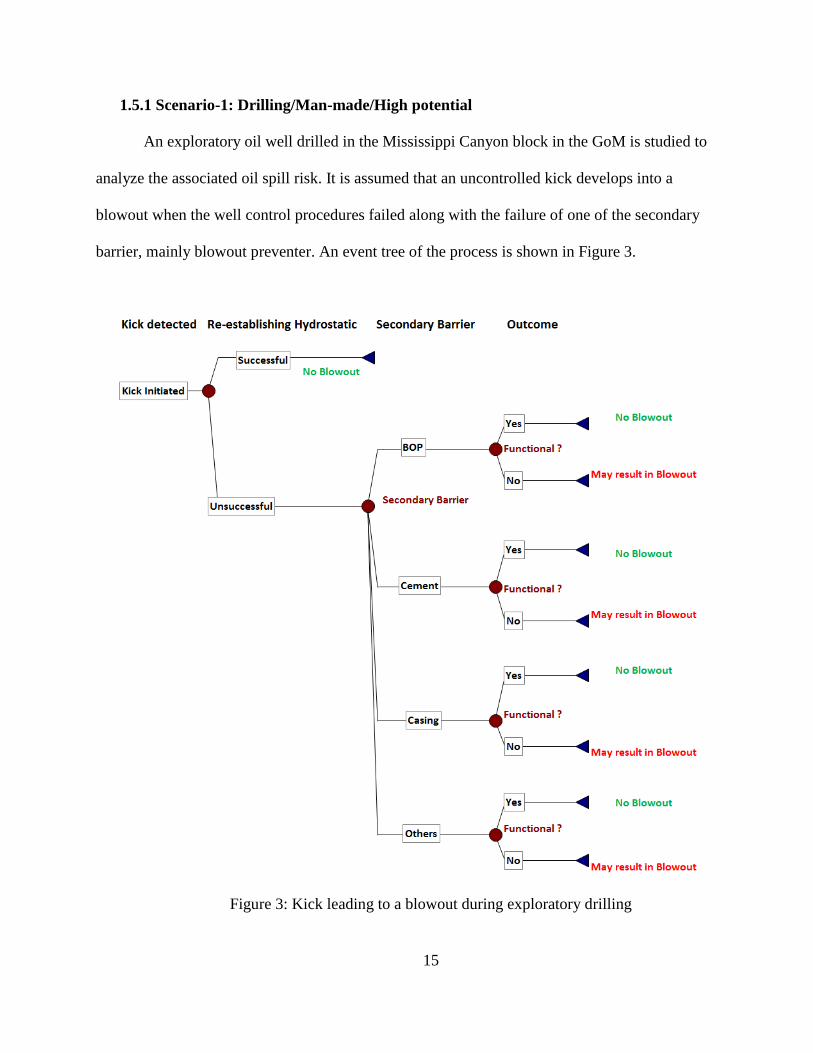
1.5.1 Scenario-1: Drilling/Man-made/High potential
An exploratory oil well drilled in the Mississippi Canyon block in the GoM is studied to
analyze the associated oil spill risk. It is assumed that an uncontrolled kick develops into a
blowout when the well control procedures failed along with the failure of one of the secondary
barrier, mainly blowout preventer. An event tree of the process is shown in Figure 3.
Figure 3: Kick leading to a blowout during exploratory drilling
16
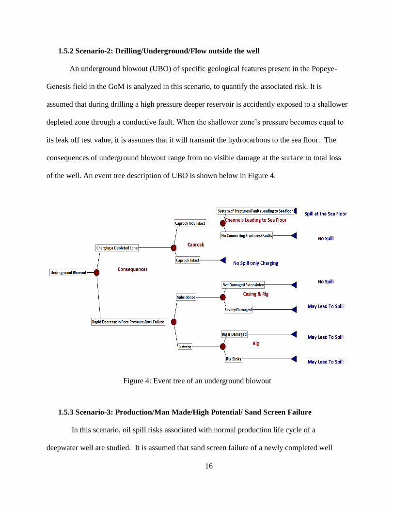
1.5.2 Scenario-2: Drilling/Underground/Flow outside the well
An underground blowout (UBO) of specific geological features present in the Popeye-
Genesis field in the GoM is analyzed in this scenario, to quantify the associated risk. It is
assumed that during drilling a high pressure deeper reservoir is accidently exposed to a shallower
depleted zone through a conductive fault. When the shallower zone’s pressure becomes equal to
its leak off test value, it is assumes that it will transmit the hydrocarbons to the sea floor. The
consequences of underground blowout range from no visible damage at the surface to total loss
of the well. An event tree description of UBO is shown below in Figure 4.
Figure 4: Event tree of an underground blowout
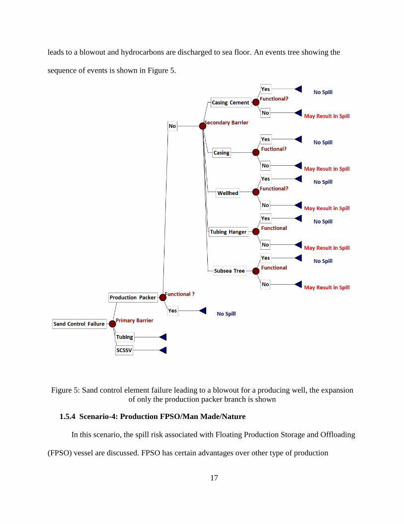
1.5.3 Scenario-3: Production/Man Made/High Potential/ Sand Screen Failure
In this scenario, oil spill risks associated with normal production life cycle of a
deepwater well are studied. It is assumed that sand screen failure of a newly completed well
17
leads to a blowout and hydrocarbons are discharged to sea floor. An events tree showing the
sequence of events is shown in Figure 5.
Figure 5: Sand control element failure leading to a blowout for a producing well, the expansion
of only the production packer branch is shown
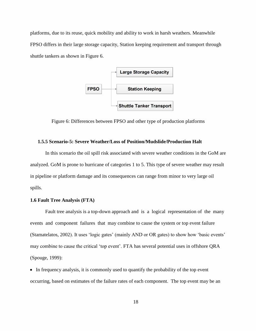
1.5.4 Scenario-4: Production FPSO/Man Made/Nature
In this scenario, the spill risk associated with Floating Production Storage and Offloading
(FPSO) vessel are discussed. FPSO has certain advantages over other type of production
18
platforms, due to its reuse, quick mobility and ability to work in harsh weathers. Meanwhile
FPSO differs in their large storage capacity, Station keeping requirement and transport through
shuttle tankers as shown in Figure 6.
Figure 6: Differences between FPSO and other type of production platforms
1.5.5 Scenario-5: Severe Weather/Loss of Position/Mudslide/Production Halt
In this scenario the oil spill risk associated with severe weather conditions in the GoM are
analyzed. GoM is prone to hurricane of categories 1 to 5. This type of severe weather may result
in pipeline or platform damage and its consequences can range from minor to very large oil
spills.
1.6 Fault Tree Analysis (FTA)
Fault tree analysis is a top-down approach and is a logical representation of the many
events and component failures that may combine to cause the system or top event failure
(Stamatelatos, 2002). It uses ‘logic gates’ (mainly AND or OR gates) to show how ‘basic events’
may combine to cause the critical ‘top event’. FTA has several potential uses in offshore QRA
(Spouge, 1999):
In frequency analysis, it is commonly used to quantify the probability of the top event
occurring, based on estimates of the failure rates of each component. The top event may be an
19
individual failure case, or a branch probability in an event tree, in this study it is the blowout
probability.
In risk presentation through importance/sensitivity analysis, it may also be used to show how
the various risk contributors combine to produce the overall risk and sensitivity of top event by
variation of basic event.
In hazard identification, it may be used qualitatively to identify combinations of basic
events that are sufficient to cause the top event, known as ‘cut sets’.
If quantification of the fault tree is the objective, downward development should stop
once all branches have been reduced to events that can be quantified. Standard symbols used in
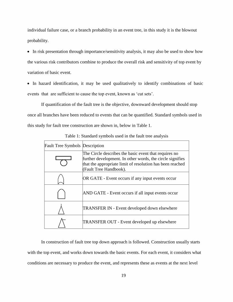
this study for fault tree construction are shown in, below in Table 1.
Table 1: Standard symbols used in the fault tree analysis
Fault Tree Symbols Description
The Circle describes the basic event that requires no
further development. In other words, the circle signifies
that the appropriate limit of resolution has been reached
(Fault Tree Handbook).
OR GATE - Event occurs if any input events occur
AND GATE - Event occurs if all input events occur
TRANSFER IN - Event developed down elsewhere
TRANSFER OUT - Event developed up elsewhere
In construction of fault tree top down approach is followed. Construction usually starts
with the top event, and works down towards the basic events. For each event, it considers what
conditions are necessary to produce the event, and represents these as events at the next level
20
down. If any one of several events may cause the higher event, they are joined with an OR gate.
If two or more events must occur in combination, they are joined with an AND gate.
1.6.1 Algebraic gate operations with probabilities
OR Gate: Consider a random experiment that can have two possible independent
outcomes A and B, which are mutually exclusive. This means that A and B cannot happen during
a single trial of the experiment. Like when we toss a coin we cannot have head and tail together.
For these mutually exclusive events, the probability of occurrence of either A and B (OR Gate) is
given by
𝑃(𝐴 𝑜𝑟𝐵) = 𝑃(𝐴) + 𝑃(𝐵)
For events that are not mutually exclusive the probability of occurrence A or B is given
by the expression
𝑃(𝐴 𝑜𝑟𝐵) = 𝑃(𝐴) + 𝑃(𝐵) − 𝑃(𝐴 𝑎𝑛𝑑 𝐵)
For three events A, B and C we have
𝑃(𝐴 𝑜𝑟 𝐵 𝑜𝑟 𝐶)
= 𝑃(𝐴) + 𝑃(𝐵) + 𝑃(𝐶) − 𝑃(𝐴 𝑎𝑛𝑑 𝐵) − 𝑃(𝐴 𝑎𝑛𝑑 𝐶) − 𝑃(𝐵 𝑎𝑛𝑑 𝐶)
+ 𝑃(𝐴 𝑎𝑛𝑑 𝐵 𝑎𝑛𝑑 𝐶)
If the PA&B is small ≤ 0.2 than 𝑃(𝐴 𝑜𝑟𝐵) = 𝑃(𝐴) + 𝑃(𝐵) with error ≤ 11%. Then this
approximation is called “rare event approximation” (Stamatelatos, 2002).
AND Gate: Now consider the two events that are mutually independent. This means that
if some experiment is performed several times, the occurrence of A has no influence on the
subsequent event B and vice versa. Then the probability of these mutually independent events
(AND Gate) is given by
𝑃(𝐴 𝑎𝑛𝑑 𝐵) = 𝑃(𝐴)𝑃(𝐵)
21
For events that are that are not mutually independent we need to use the concept of
conditional probability. For example 𝑃(𝐵|𝐴) is the probability of event B, given that event A has
already taken place.
𝑃(𝐴 𝑎𝑛𝑑 𝐵) = 𝑃(𝐴)𝑃(𝐵|𝐴) = 𝑃(𝐵)𝑃(𝐴|𝐵)
If A and B are mutually independent, then 𝑃(𝐴|𝐵) = 𝑃(𝐴) and𝑃(𝐵|𝐴) = 𝑃(𝐵).
1.7 Reliability Analysis
The science of reliability prediction is based upon the principals of statistical analysis.
Reliability is defined as “the probability that equipment will perform a specified function
under stated conditions for a given period of time” which defines a probabilistic
approach rather than a deterministic one. This probability can be calculated or stated to reside
within certain statistical confidence limits. To calculate the reliability of the system, its failure
rate or Mean Time to Failure (MTTF) and /or the Probability of Failure on Demand (PDF) are
needed. The most comprehensive subsea equipment reliability data is available through OREDA
(Offshore Reliability Data) database software containing the latest data available. The OREDA
2009 Handbook contains offshore subsea and topside equipment reliability data till 2003, from
which some of the equipment reliability data is used in this study. As there is increased activity
in the past few years in deepwater, so use of data from OREDA online database will provide
more accurate results as compared to using the OREDA handbook data.
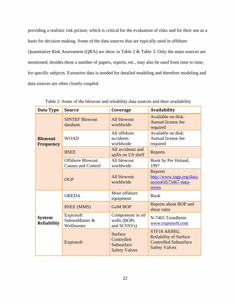
1.8 Data Sources
Blowouts are one of the main risks associated with the exploration and production
operations in deepwaters. The quality check of the input data is an important aspect required to
ensure a satisfactory quality risk analysis procedure. Good input data quality will result in
22
providing a realistic risk picture, which is critical for the evaluation of risks and for their use as a
basis for decision making. Some of the data sources that are typically used in offshore
Quantitative Risk Assessment (QRA) are show in Table 2 & Table 3. Only the main sources are
mentioned, besides these a number of papers, reports, etc., may also be used from time to time,
for specific subjects. Extensive data is needed for detailed modeling and therefore modeling and
data sources are often closely coupled.
Table 2: Some of the blowout and reliability data sources and their availability
Data Type Source Coverage Availability
Blowout Frequency
SINTEF Blowout
database
All blowout
worldwide
Available on disk:
Annual license fee
required
WOAD
All offshore
accidents
worldwide
Available on disk:
Annual license fee
required
BSEE All accidents and
spills on US shelf Reports
Offshore Blowout
Causes and Control
All blowout
worldwide
Book by Per Holand,
1997
OGP All blowout
worldwide
Reports
http://www.iogp.org/data-
series#2673467-data-
series
System Reliability
OREDA Most offshore
equipment Book
BSEE (MMS) GoM BOP Reports about BOP and
shear rams
Exprosoft
SubseaMaster &
Wellmaster
Components in oil
wells (BOPs
and SCSSVs)
N-7465 Trondheim
www.exprosoft.com
Exprosoft
Surface
Controlled
Subsurface
Safety Valves
STF18 A83002,
Reliability of Surface
Controlled Subsurface
Safety Valves
23
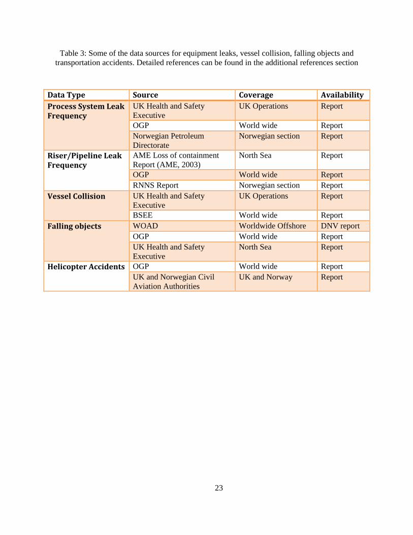
Table 3: Some of the data sources for equipment leaks, vessel collision, falling objects and
transportation accidents. Detailed references can be found in the additional references section
Data Type Source Coverage Availability
Process System Leak Frequency
UK Health and Safety
Executive
UK Operations Report
OGP World wide Report
Norwegian Petroleum
Directorate
Norwegian section Report
Riser/Pipeline Leak Frequency
AME Loss of containment
Report (AME, 2003)
North Sea Report
OGP World wide Report
RNNS Report Norwegian section Report
Vessel Collision
UK Health and Safety
Executive
UK Operations Report
BSEE World wide Report
Falling objects
WOAD Worldwide Offshore DNV report
OGP World wide Report
UK Health and Safety
Executive
North Sea Report
Helicopter Accidents
OGP World wide Report
UK and Norwegian Civil
Aviation Authorities
UK and Norway Report
24
CHAPTER 2: FRAMEWORK FOR RISK ASSESSMENT PROCESS
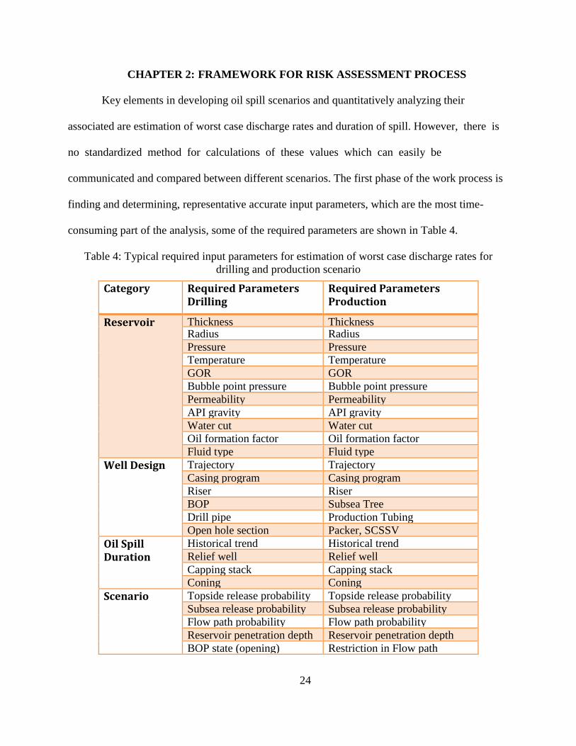
Key elements in developing oil spill scenarios and quantitatively analyzing their
associated are estimation of worst case discharge rates and duration of spill. However, there is
no standardized method for calculations of these values which can easily be
communicated and compared between different scenarios. The first phase of the work process is
finding and determining, representative accurate input parameters, which are the most time-
consuming part of the analysis, some of the required parameters are shown in Table 4.
Table 4: Typical required input parameters for estimation of worst case discharge rates for
drilling and production scenario
Category Required Parameters Drilling
Required Parameters Production
Reservoir
Thickness Thickness Radius Radius
Pressure Pressure
Temperature Temperature
GOR GOR
Bubble point pressure Bubble point pressure
Permeability Permeability
API gravity API gravity
Water cut Water cut
Oil formation factor Oil formation factor
Fluid type Fluid type
Well Design
Trajectory Trajectory
Casing program Casing program
Riser Riser
BOP Subsea Tree
Drill pipe Production Tubing
Open hole section Packer, SCSSV
Oil Spill Duration
Historical trend Historical trend
Relief well Relief well
Capping stack Capping stack
Coning Coning
Scenario
Topside release probability Topside release probability
Subsea release probability Subsea release probability
Flow path probability Flow path probability
Reservoir penetration depth Reservoir penetration depth
BOP state (opening) Restriction in Flow path
25
Here parameters such as representative well location, well geometry, reservoir properties,
spill response technologies and probabilities of different blowout scenarios must be accurately
determined for true representation of the regional properties. This data must be carefully
considered to achieve as accurate results as possible.
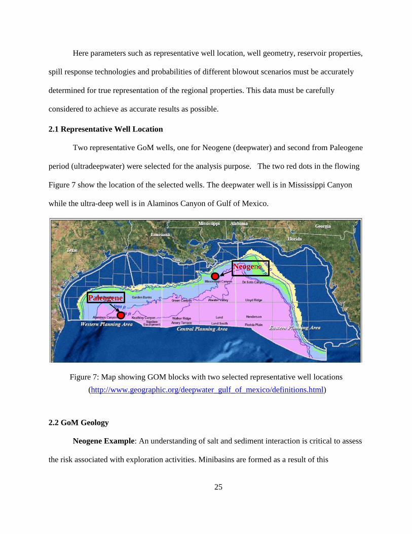
2.1 Representative Well Location
Two representative GoM wells, one for Neogene (deepwater) and second from Paleogene
period (ultradeepwater) were selected for the analysis purpose. The two red dots in the flowing
Figure 7 show the location of the selected wells. The deepwater well is in Mississippi Canyon
while the ultra-deep well is in Alaminos Canyon of Gulf of Mexico.
Figure 7: Map showing GOM blocks with two selected representative well locations
(http://www.geographic.org/deepwater_gulf_of_mexico/definitions.html)
2.2 GoM Geology
Neogene Example: An understanding of salt and sediment interaction is critical to assess
the risk associated with exploration activities. Minibasins are formed as a result of this
Neogene
Paleogene
26
interaction. The Neogene geology of GoM can be categorized in four major groups of Plio-
Pleistocene Fluvial Sandstone, Upper Miocene Deltaic Sandstone, Middle Miocene Deltaic
Sandstone and Lower Miocene Slope and Fan Sandstone. The source rock for these plays is the
deep upper Jurassic and through vertical migratory paths, hydrocarbons travelled and trapped by
these low lying Neogene traps. Some of the faults in these plays are nearly horizontal and they
sometime provide barriers to the flowing fluid and help in trapping the migratory hydrocarbons.
Most of these sands are not very thick and multiple sands are stacked as well.
Paleogene Wilcox Example: Deepwater Gulf of Mexico contains numerous geologic
plays at different reservoir depths with proven hydrocarbon resource. Among these plays is the
Wilcox, where exploration and appraisal drilling has increased since 2001, and reported
successes indicate that the play holds significant producible hydrocarbons in the order of multi-
billion barrels. However, depth, location, and reservoir characteristics of the offshore Wilcox
play present various challenges to commercial development of the Wilcox formation even with
today’s technology (Joshua Oletu etal. 2013). The deepwater GOM Wilcox trend comprises
Upper (or Late) Paleocene to Lower (or Early) Eocene age fan turbidites that stretch over some
400 miles from Alaminos Canyon in the west to Atwater Valley in the east. The Wilcox is a
subunit of the Lower Tertiary system. The dominant sediment source is believed to be onshore
deltaic, with clastic sediments deposited in a complex slope system, resulting in minibasins and
base of slope fans.
2.3 Representative reservoir properties
Representative reservoir sand properties both for Paleogene and Neogene reservoirs are
briefly described in the following sections.
27
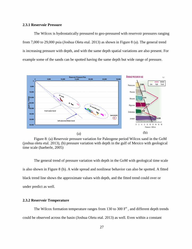
2.3.1 Reservoir Pressure
The Wilcox is hydrostatically pressured to geo-pressured with reservoir pressures ranging
from 7,000 to 29,000 psia (Joshua Oletu etal. 2013) as shown in Figure 8 (a). The general trend
is increasing pressure with depth, and with the same depth spatial variations are also present. For
example some of the sands can be spotted having the same depth but wide range of pressure.
Figure 8: (a) Reservoir pressure variation for Paleogene period Wilcox sand in the GoM
(joshua oletu etal. 2013), (b) pressure variation with depth in the gulf of Mexico with geological
time scale (haeberle, 2005)
The general trend of pressure variation with depth in the GoM with geological time scale
is also shown in Figure 8 (b). A wide spread and nonlinear behavior can also be spotted. A fitted
black trend line shows the approximate values with depth, and the fitted trend could over or
under predict as well.
2.3.2 Reservoir Temperature
The Wilcox formation temperature ranges from 130 to 300 Fo , and different depth trends
could be observed across the basin (Joshua Oletu etal. 2013) as well. Even within a constant
(
b)
(
a)
(b) (a)
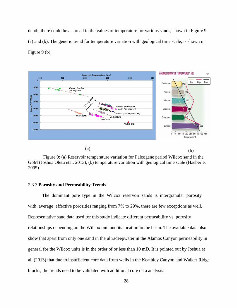
28
depth, there could be a spread in the values of temperature for various sands, shown in Figure 9
(a) and (b). The generic trend for temperature variation with geological time scale, is shown in
Figure 9 (b).
Figure 9: (a) Reservoir temperature variation for Paleogene period Wilcox sand in the
GoM (Joshua Oletu etal. 2013), (b) temperature variation with geological time scale (Haeberle,
2005)
2.3.3 Porosity and Permeability Trends
The dominant pore type in the Wilcox reservoir sands is intergranular porosity
with average effective porosities ranging from 7% to 29%, there are few exceptions as well.
Representative sand data used for this study indicate different permeability vs. porosity
relationships depending on the Wilcox unit and its location in the basin. The available data also
show that apart from only one sand in the ultradeepwater in the Alamos Canyon permeability in
general for the Wilcox units is in the order of or less than 10 mD. It is pointed out by Joshua et
al. (2013) that due to insufficient core data from wells in the Keathley Canyon and Walker Ridge
blocks, the trends need to be validated with additional core data analysis.
(a) (b)
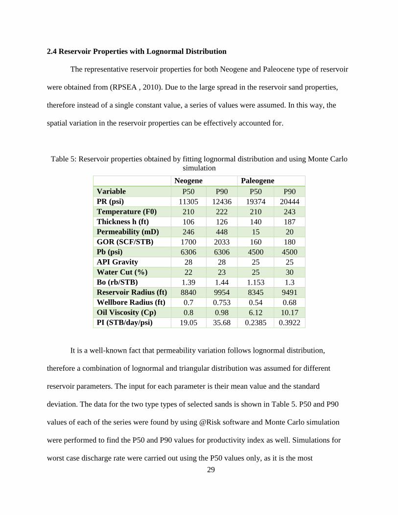
29
2.4 Reservoir Properties with Lognormal Distribution
The representative reservoir properties for both Neogene and Paleocene type of reservoir
were obtained from (RPSEA , 2010). Due to the large spread in the reservoir sand properties,
therefore instead of a single constant value, a series of values were assumed. In this way, the
spatial variation in the reservoir properties can be effectively accounted for.
Table 5: Reservoir properties obtained by fitting lognormal distribution and using Monte Carlo
simulation
Neogene Paleogene
Variable P50 P90 P50 P90
PR (psi) 11305 12436 19374 20444
Temperature (F0) 210 222 210 243
Thickness h (ft) 106 126 140 187
Permeability (mD) 246 448 15 20
GOR (SCF/STB) 1700 2033 160 180
Pb (psi) 6306 6306 4500 4500
API Gravity 28 28 25 25
Water Cut (%) 22 23 25 30
Bo (rb/STB) 1.39 1.44 1.153 1.3
Reservoir Radius (ft) 8840 9954 8345 9491
Wellbore Radius (ft) 0.7 0.753 0.54 0.68
Oil Viscosity (Cp) 0.8 0.98 6.12 10.17
PI (STB/day/psi) 19.05 35.68 0.2385 0.3922
It is a well-known fact that permeability variation follows lognormal distribution,
therefore a combination of lognormal and triangular distribution was assumed for different
reservoir parameters. The input for each parameter is their mean value and the standard
deviation. The data for the two type types of selected sands is shown in Table 5. P50 and P90
values of each of the series were found by using @Risk software and Monte Carlo simulation
were performed to find the P50 and P90 values for productivity index as well. Simulations for
worst case discharge rate were carried out using the P50 values only, as it is the most
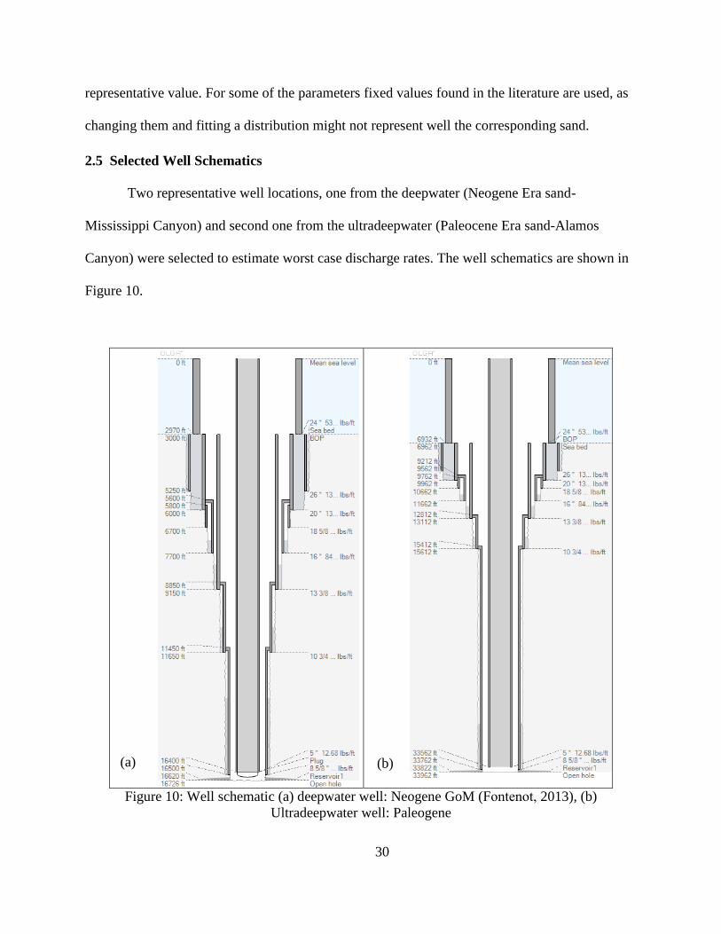
30
representative value. For some of the parameters fixed values found in the literature are used, as
changing them and fitting a distribution might not represent well the corresponding sand.
2.5 Selected Well Schematics
Two representative well locations, one from the deepwater (Neogene Era sand-
Mississippi Canyon) and second one from the ultradeepwater (Paleocene Era sand-Alamos
Canyon) were selected to estimate worst case discharge rates. The well schematics are shown in
Figure 10.
Figure 10: Well schematic (a) deepwater well: Neogene GoM (Fontenot, 2013), (b)
Ultradeepwater well: Paleogene
(a) (b)
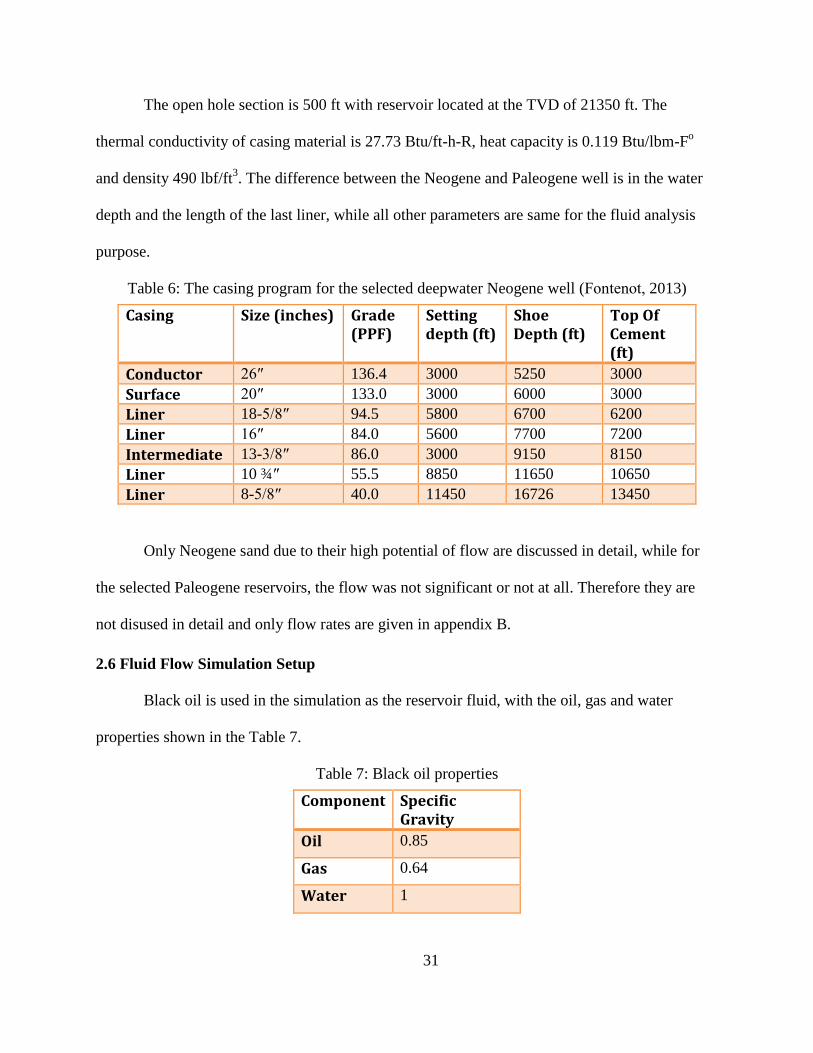
31
The open hole section is 500 ft with reservoir located at the TVD of 21350 ft. The
thermal conductivity of casing material is 27.73 Btu/ft-h-R, heat capacity is 0.119 Btu/lbm-Fo
and density 490 lbf/ft3. The difference between the Neogene and Paleogene well is in the water
depth and the length of the last liner, while all other parameters are same for the fluid analysis
purpose.
Table 6: The casing program for the selected deepwater Neogene well (Fontenot, 2013)
Casing Size (inches) Grade (PPF)
Setting depth (ft)
Shoe Depth (ft)
Top Of Cement (ft)
Conductor 26″ 136.4 3000 5250 3000
Surface 20″ 133.0 3000 6000 3000
Liner 18-5/8″ 94.5 5800 6700 6200
Liner 16″ 84.0 5600 7700 7200
Intermediate 13-3/8″ 86.0 3000 9150 8150
Liner 10 ¾″ 55.5 8850 11650 10650
Liner 8-5/8″ 40.0 11450 16726 13450
Only Neogene sand due to their high potential of flow are discussed in detail, while for
the selected Paleogene reservoirs, the flow was not significant or not at all. Therefore they are
not disused in detail and only flow rates are given in appendix B.
2.6 Fluid Flow Simulation Setup
Black oil is used in the simulation as the reservoir fluid, with the oil, gas and water
properties shown in the Table 7.
Table 7: Black oil properties
Component Specific Gravity
Oil 0.85
Gas 0.64
Water 1
32
Temperature Profile: The sea water temper decreases with water depth from 79 Fo at the
sea surface to nearly 40 Fo at 3,000 ft depth selected for deepwater Neogene well. Below the
mud line a linear geothermal gradient was assumed with 40 Fo at mudline and then temperature
linearly increases with depth to 210 Fo at the target depth of 21350 ft.
Inflow Performance Relationship (IPR)
Two component IPR was used with linear profile for PR > Pb and quadratic for the case if
PR < Pb.
𝑞 = 𝐽(𝑃𝑅 − 𝑃𝑤𝑓) for 𝑃𝑏 ≤ 𝑃𝑤𝑓 ≤ 𝑃𝑅
where q is the volumetric flow rate, PR is reservoir pressure, J is productivity index, and
Pwf is the well flowing pressure.
𝑞 = 𝐽(𝑃𝑅 − 𝑃𝑏) + (𝐽
2𝑃𝑏) (𝑃𝑏
2 − 𝑃𝑤𝑓2) for 𝑃𝑤𝑓 ≤ 𝑃𝑏
where Pb is the bubble point pressure. The productivity index for pseudo steady state
flow is given by
𝐽 =0.007082𝑘ℎ
𝐵𝑜𝜇𝑜 [𝑙𝑛𝑟𝑒
𝑟𝑤+ 𝑠 − 0.75]
(1)
where k: permeability (mD), h: reservoir thickness (ft), re: reservoir radius (ft), rw:
wellbore radius (ft), s: skin, μo: oil viscosity (cp), βo : oil formation factor
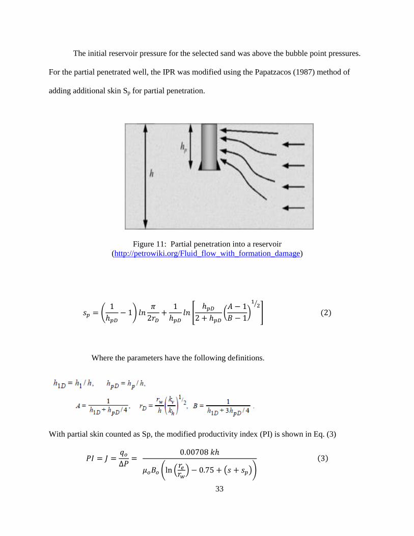
33
The initial reservoir pressure for the selected sand was above the bubble point pressures.
For the partial penetrated well, the IPR was modified using the Papatzacos (1987) method of
adding additional skin Sp for partial penetration.
Figure 11: Partial penetration into a reservoir
(http://petrowiki.org/Fluid_flow_with_formation_damage)
𝑠𝑝 = (1
ℎ𝑝𝐷− 1) 𝑙𝑛
𝜋
2𝑟𝐷+
1
ℎ𝑝𝐷𝑙𝑛 [
ℎ𝑝𝐷
2 + ℎ𝑝𝐷(
𝐴 − 1
𝐵 − 1)
12⁄
] (2)
Where the parameters have the following definitions.
With partial skin counted as Sp, the modified productivity index (PI) is shown in Eq. (3)
𝑃𝐼 = 𝐽 =𝑞𝑜
∆𝑃=
0.00708 𝑘ℎ
𝜇𝑜𝐵𝑜 (ln (𝑟𝑒
𝑟𝑤) − 0.75 + (𝑠 + 𝑠𝑝))
(3)
34
Reservoir Pressure Decline
The reservoir pressure decline can be estimated, by using the material balance equation
under the assumption that the reservoir is bounded with no aquifer support to maintain the
pressure and production occurs due to expansion of the reservoir fluids only. The material
balance results in the equation (4)
𝑃𝑡 = 𝑃𝑖 −𝑁𝑝 𝐵𝑜
𝐶𝑡𝑁𝑖 (4)
Where
Pt is the pressure at time t
Pi is the initial reservoir Pressure
Np produced oil volume
Ni original oil in place
Ct total reservoir compressibility
Bo oil formation volume factor
Total reservoir compressibility is calculated by using Hall’s correlation
𝐶𝑡 = 1.87 × 10⁻⁶𝜑−0.415
and change in porosity can be estimated as
𝜑 = 𝜑𝑜𝑒𝑥𝑝[𝐶𝑡(𝑝𝑡 − 𝑝𝑖)]
Standing Correlation was used to calculate oil formation volume factor.
35
CHAPTER 3: OIL SPILL RISK ASSESSMENT OF A DEEPWATER EXPLORATORY
DRILLING WELL (SCENARIO-1)
Major offshore accidents such as Macondo well incident highlight one of the possible
failure modes and subsequent disasters when an offshore engineering project could go wrong.
Such events can happen during any life phase of an offshore well - starting from the exploratory
drilling phase to the final phase of plug and abandonment, but their potential to cause major
environmental damage is greatest in their early life phase. Major factors that significantly
contribute in defining such accident scenarios are the geological and operational complexities,
equipment reliability, human factors, geographical/economy location, and weather conditions.
The path taken by the reservoir fluids to reach the sea floor is also an important factor in
determining the worst case discharge rates, as different paths provide different resistances to
flowing fluid. Environmental risk of an oil/gas spill is also a function of the type of hydrocarbons
released and amount of oil volume spilled.
A representative well from Mississippi Canyon in the Gulf of Mexico is studied for
quantitative risk assessment (QRA) of an oil spill in the exploratory life phase of a well. At the
location of the well, sea water depth is 3,000 ft and total vertical depth of reservoir is 16,726 ft.
The reservoir sand is associated with Neogene geological period and representative reservoir
properties for this well are selected from literature. Due to the large spatial variation of reservoir
properties, a single selected value will not truly represent the general behavior in that particular
area, therefore a spread of values should be considered. In this study, this spread is in the form of
lognormal & triangular distributions. From these distributions P10, P50 and P90 values can be
obtained. To find representative value for productivity index, the variables were entered in the
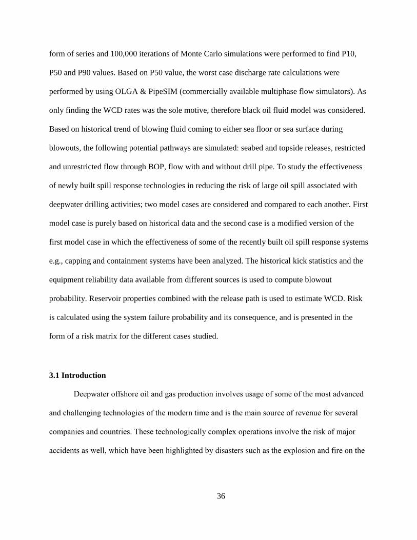
36
form of series and 100,000 iterations of Monte Carlo simulations were performed to find P10,
P50 and P90 values. Based on P50 value, the worst case discharge rate calculations were
performed by using OLGA & PipeSIM (commercially available multiphase flow simulators). As
only finding the WCD rates was the sole motive, therefore black oil fluid model was considered.
Based on historical trend of blowing fluid coming to either sea floor or sea surface during
blowouts, the following potential pathways are simulated: seabed and topside releases, restricted
and unrestricted flow through BOP, flow with and without drill pipe. To study the effectiveness
of newly built spill response technologies in reducing the risk of large oil spill associated with
deepwater drilling activities; two model cases are considered and compared to each another. First
model case is purely based on historical data and the second case is a modified version of the
first model case in which the effectiveness of some of the recently built oil spill response systems
e.g., capping and containment systems have been analyzed. The historical kick statistics and the
equipment reliability data available from different sources is used to compute blowout
probability. Reservoir properties combined with the release path is used to estimate WCD. Risk
is calculated using the system failure probability and its consequence, and is presented in the
form of a risk matrix for the different cases studied.
3.1 Introduction
Deepwater offshore oil and gas production involves usage of some of the most advanced
and challenging technologies of the modern time and is the main source of revenue for several
companies and countries. These technologically complex operations involve the risk of major
accidents as well, which have been highlighted by disasters such as the explosion and fire on the
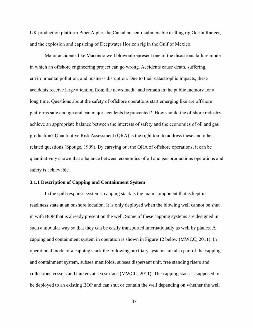
37
UK production platform Piper Alpha, the Canadian semi-submersible drilling rig Ocean Ranger,
and the explosion and capsizing of Deepwater Horizon rig in the Gulf of Mexico.
Major accidents like Macondo well blowout represent one of the disastrous failure mode
in which an offshore engineering project can go wrong. Accidents cause death, suffering,
environmental pollution, and business disruption. Due to their catastrophic impacts, these
accidents receive large attention from the news media and remain in the public memory for a
long time. Questions about the safety of offshore operations start emerging like are offshore
platforms safe enough and can major accidents be prevented? How should the offshore industry
achieve an appropriate balance between the interests of safety and the economics of oil and gas
production? Quantitative Risk Assessment (QRA) is the right tool to address these and other
related questions (Spouge, 1999). By carrying out the QRA of offshore operations, it can be
quantitatively shown that a balance between economics of oil and gas productions operations and
safety is achievable.
3.1.1 Description of Capping and Containment System
In the spill response systems, capping stack is the main component that is kept in
readiness state at an onshore location. It is only deployed when the blowing well cannot be shut
in with BOP that is already present on the well. Some of these capping systems are designed in
such a modular way so that they can be easily transported internationally as well by planes. A
capping and containment system in operation is shown in Figure 12 below (MWCC, 2011). In
operational mode of a capping stack the following auxiliary systems are also part of the capping
and containment system, subsea manifolds, subsea dispersant unit, free standing risers and
collections vessels and tankers at sea surface (MWCC, 2011). The capping stack is supposed to
be deployed to an existing BOP and can shut or contain the well depending on whether the well
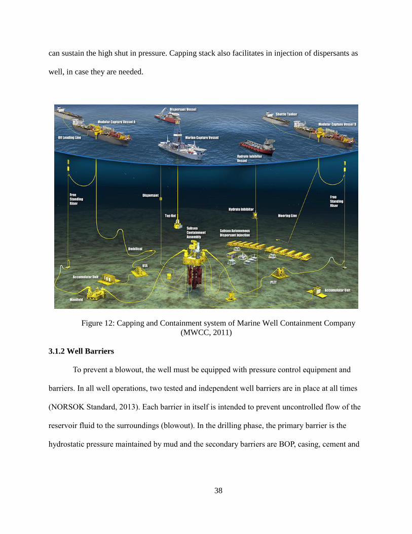
38
can sustain the high shut in pressure. Capping stack also facilitates in injection of dispersants as
well, in case they are needed.
Figure 12: Capping and Containment system of Marine Well Containment Company
(MWCC, 2011)
3.1.2 Well Barriers
To prevent a blowout, the well must be equipped with pressure control equipment and
barriers. In all well operations, two tested and independent well barriers are in place at all times
(NORSOK Standard, 2013). Each barrier in itself is intended to prevent uncontrolled flow of the
reservoir fluid to the surroundings (blowout). In the drilling phase, the primary barrier is the
hydrostatic pressure maintained by mud and the secondary barriers are BOP, casing, cement and

39
wellhead seals. A blowout can only occur when both of these barriers fails simultaneously. These
barriers are shown in Figure 13.
Figure 13: Primary and secondary barriers in a drilling well (NORSOK Standard, 2013)
3.1.3 Methodology
In order to calculate the quantified risk, the incident’s probability/frequency and its
consequences are required. The incident frequency is computed from Fault Tree Analysis, while
consequences in the form of oil volume released to the environment are found from multiphase
fluid flow analysis in wellbore.
3.1.4 Representative Well, Reservoir Properties, and QRA Procedure
Representative properties for a reservoir corresponding to the selected well’s location are
taken from literature (RPSEA, 2010) and are shown in Figure 14, alongside the result of fitted
distributions and Monte Carlo simulations.
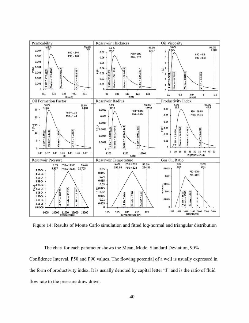
40
Permeability Reservoir Thickness Oil Viscosity
Oil Formation Factor Reservoir Radius Productivity Index
Reservoir Pressure Reservoir Temperature Gas Oil Ratio
Figure 14: Results of Monte Carlo simulation and fitted log-normal and triangular distribution
The chart for each parameter shows the Mean, Mode, Standard Deviation, 90%
Confidence Interval, P50 and P90 values. The flowing potential of a well is usually expressed in
the form of productivity index. It is usually denoted by capital letter “J” and is the ratio of fluid
flow rate to the pressure draw down.
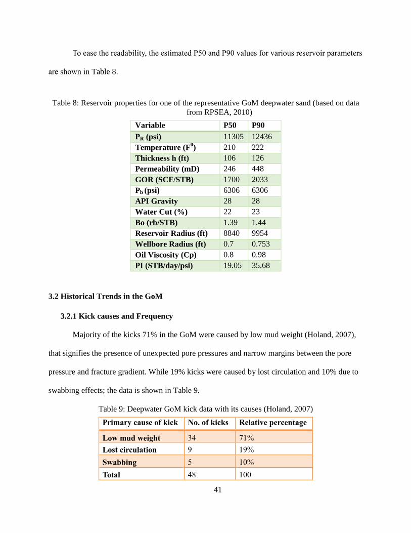
41
To ease the readability, the estimated P50 and P90 values for various reservoir parameters
are shown in Table 8.
Table 8: Reservoir properties for one of the representative GoM deepwater sand (based on data
from RPSEA, 2010)
Variable P50 P90
PR (psi) 11305 12436
Temperature (F0) 210 222
Thickness h (ft) 106 126
Permeability (mD) 246 448
GOR (SCF/STB) 1700 2033
Pb (psi) 6306 6306
API Gravity 28 28
Water Cut (%) 22 23
Bo (rb/STB) 1.39 1.44
Reservoir Radius (ft) 8840 9954
Wellbore Radius (ft) 0.7 0.753
Oil Viscosity (Cp) 0.8 0.98
PI (STB/day/psi) 19.05 35.68
3.2 Historical Trends in the GoM
3.2.1 Kick causes and Frequency
Majority of the kicks 71% in the GoM were caused by low mud weight (Holand, 2007),
that signifies the presence of unexpected pore pressures and narrow margins between the pore
pressure and fracture gradient. While 19% kicks were caused by lost circulation and 10% due to
swabbing effects; the data is shown in Table 9.
Table 9: Deepwater GoM kick data with its causes (Holand, 2007)
Primary cause of kick No. of kicks Relative percentage
Low mud weight 34 71%
Lost circulation 9 19%
Swabbing 5 10%
Total 48 100
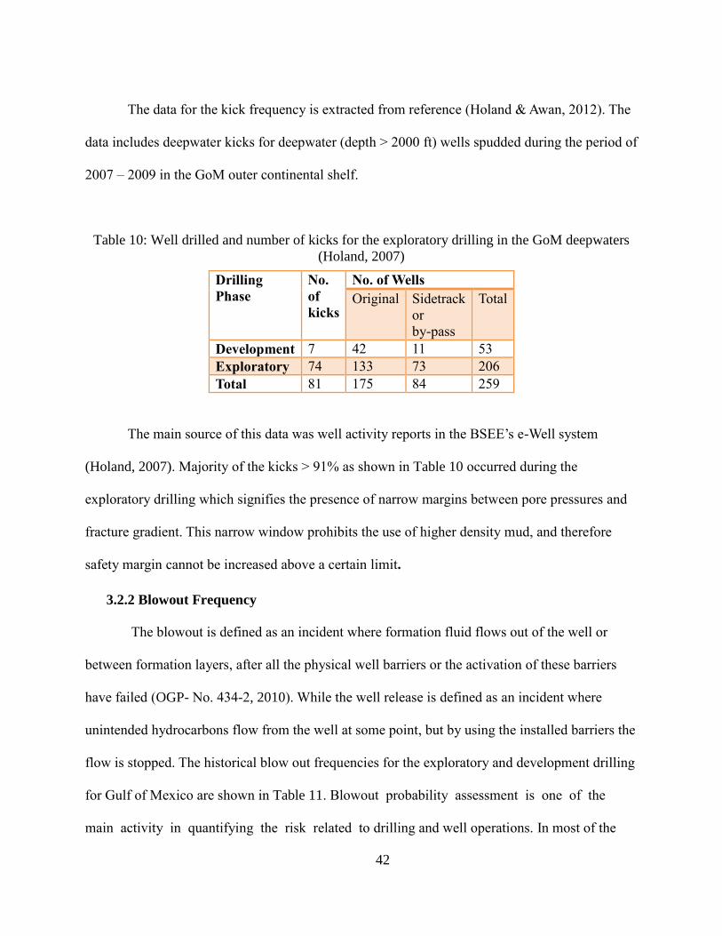
42
The data for the kick frequency is extracted from reference (Holand & Awan, 2012). The
data includes deepwater kicks for deepwater (depth > 2000 ft) wells spudded during the period of
2007 – 2009 in the GoM outer continental shelf.
Table 10: Well drilled and number of kicks for the exploratory drilling in the GoM deepwaters
(Holand, 2007)
Drilling
Phase
No.
of
kicks
No. of Wells
Original Sidetrack
or
by-pass
Total
Development 7 42 11 53
Exploratory 74 133 73 206
Total 81 175 84 259
The main source of this data was well activity reports in the BSEE’s e-Well system
(Holand, 2007). Majority of the kicks > 91% as shown in Table 10 occurred during the
exploratory drilling which signifies the presence of narrow margins between pore pressures and
fracture gradient. This narrow window prohibits the use of higher density mud, and therefore
safety margin cannot be increased above a certain limit.
3.2.2 Blowout Frequency
The blowout is defined as an incident where formation fluid flows out of the well or
between formation layers, after all the physical well barriers or the activation of these barriers
have failed (OGP- No. 434-2, 2010). While the well release is defined as an incident where
unintended hydrocarbons flow from the well at some point, but by using the installed barriers the
flow is stopped. The historical blow out frequencies for the exploratory and development drilling
for Gulf of Mexico are shown in Table 11. Blowout probability assessment is one of the
main activity in quantifying the risk related to drilling and well operations. In most of the
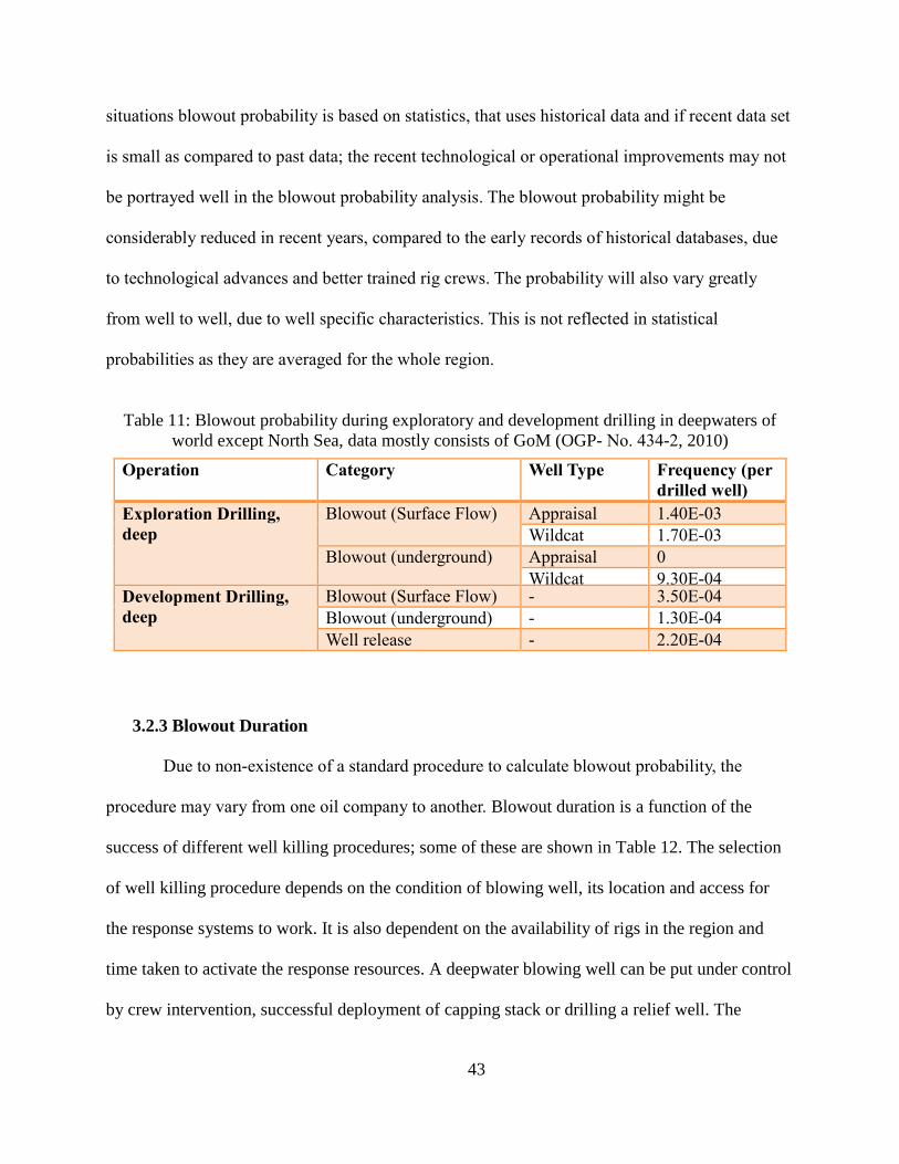
43
situations blowout probability is based on statistics, that uses historical data and if recent data set
is small as compared to past data; the recent technological or operational improvements may not
be portrayed well in the blowout probability analysis. The blowout probability might be
considerably reduced in recent years, compared to the early records of historical databases, due
to technological advances and better trained rig crews. The probability will also vary greatly
from well to well, due to well specific characteristics. This is not reflected in statistical
probabilities as they are averaged for the whole region.
Table 11: Blowout probability during exploratory and development drilling in deepwaters of
world except North Sea, data mostly consists of GoM (OGP- No. 434-2, 2010)
Operation Category Well Type Frequency (per
drilled well)
Exploration Drilling,
deep
Blowout (Surface Flow) Appraisal 1.40E-03
Wildcat 1.70E-03
Blowout (underground) Appraisal 0
Wildcat 9.30E-04 Development Drilling,
deep
Blowout (Surface Flow) - 3.50E-04
Blowout (underground) - 1.30E-04
Well release - 2.20E-04
3.2.3 Blowout Duration
Due to non-existence of a standard procedure to calculate blowout probability, the
procedure may vary from one oil company to another. Blowout duration is a function of the
success of different well killing procedures; some of these are shown in Table 12. The selection
of well killing procedure depends on the condition of blowing well, its location and access for
the response systems to work. It is also dependent on the availability of rigs in the region and
time taken to activate the response resources. A deepwater blowing well can be put under control
by crew intervention, successful deployment of capping stack or drilling a relief well. The
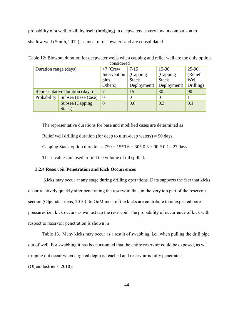
44
probability of a well to kill by itself (bridging) in deepwaters is very low in comparison to
shallow well (Smith, 2012), as most of deepwater sand are consolidated.
Table 12: Blowout duration for deepwater wells when capping and relief well are the only option
considered
Duration range (days) <7 (Crew
Intervention
plus
Others)
7-15
(Capping
Stack
Deployment)
15-30
(Capping
Stack
Deployment)
25-90
(Relief
Well
Drilling)
Representative duration (days) 7 15 30 90
Probability Subsea (Base Case) 0 0 0 1
Subsea (Capping
Stack)
0 0.6 0.3 0.1
The representative durations for base and modified cases are determined as
Relief well drilling duration (for deep to ultra-deep waters) = 90 days
Capping Stack option duration = 7*0 + 15*0.6 + 30* 0.3 + 90 * 0.1= 27 days
These values are used to find the volume of oil spilled.
3.2.4 Reservoir Penetration and Kick Occurrences
Kicks may occur at any stage during drilling operations. Data supports the fact that kicks
occur relatively quickly after penetrating the reservoir, thus in the very top part of the reservoir
section (Oljeindustriens, 2010). In GoM most of the kicks are contribute to unexpected pore
pressures i.e., kick occurs as we just tap the reservoir. The probability of occurrence of kick with
respect to reservoir penetration is shown in
Table 13. Many kicks may occur as a result of swabbing, i.e., when pulling the drill pipe
out of well. For swabbing it has been assumed that the entire reservoir could be exposed, as we
tripping out occur when targeted depth is reached and reservoir is fully penetrated
(Oljeindustriens, 2010).
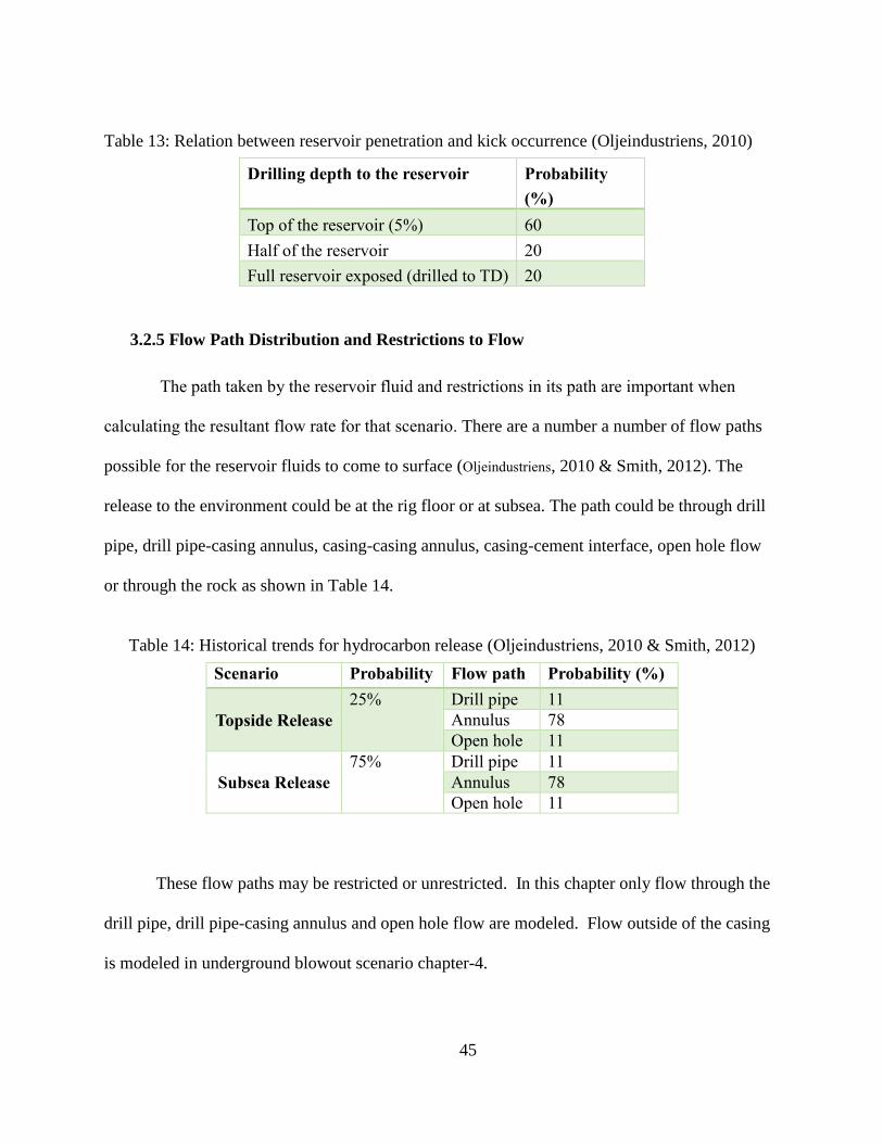
45
Table 13: Relation between reservoir penetration and kick occurrence (Oljeindustriens, 2010)
Drilling depth to the reservoir Probability
(%)
Top of the reservoir (5%) 60
Half of the reservoir 20
Full reservoir exposed (drilled to TD) 20
3.2.5 Flow Path Distribution and Restrictions to Flow
The path taken by the reservoir fluid and restrictions in its path are important when
calculating the resultant flow rate for that scenario. There are a number a number of flow paths
possible for the reservoir fluids to come to surface (Oljeindustriens, 2010 & Smith, 2012). The
release to the environment could be at the rig floor or at subsea. The path could be through drill
pipe, drill pipe-casing annulus, casing-casing annulus, casing-cement interface, open hole flow
or through the rock as shown in Table 14.
Table 14: Historical trends for hydrocarbon release (Oljeindustriens, 2010 & Smith, 2012)
Scenario Probability Flow path Probability (%)
Topside Release
25% Drill pipe 11
Annulus 78
Open hole 11
Subsea Release
75% Drill pipe 11
Annulus 78
Open hole 11
These flow paths may be restricted or unrestricted. In this chapter only flow through the
drill pipe, drill pipe-casing annulus and open hole flow are modeled. Flow outside of the casing
is modeled in underground blowout scenario chapter-4.
46
3.2.6 Flow Rate, Spill Duration and Fault Tree Analysis
Commercially available multiphase fluid flow simulators PipeSim & OLGA were used to
find the worst case discharge rate under different conditions. A linear geothermal gradient was
assumed with well’s surrounding temperature at mud line of 40Fo and reaching to 210F
o at the
reservoir depth. The specific gravities of oil, gas and water were taken to be 0.86, 0.67 and 1
respectively. The viscosity was modeled using Vasquez & Beggs (1980) correlation. The
roughness of wellbore and casing and drill pipe was assumed to be 0.001 inches. The overall heat
transfer coefficient was taken as 2 Btu/hr/ft2 of a steel pipe. The back pressure at the fluid outlet
at seabed is fixed to be 1395 psi based on the average sea water gradient of 0.465 psi/ft for the
Gulf of Mexico with a water depth of 3000 ft.
The kick and the BOP equipment reliability data for Fault Tree Analysis are extracted
from (MIDE, 2010), which is based on SINTEF Offshore Blowout Database (SINTEF, 2001).
The failure rate of each of secondary barrier is assumed to be a uniform average rate with ± 10%
spread in value and is expressed as failures per drilled well. In contrary to normal fault tree
analysis where top event’s frequency (blowout in this case) is to be found, based on the failure
rates of basic events, in this case the top event probability is also known. The tree is calibrated in
such a way that to obtain the same blowout frequency, the frequency of only well control
procedures is adjusted while all other basic event frequencies are not disturbed and they
represent the failure rates of those components, mentioned in the literature. Although a crude
assumptions, all the basic events are treated as independent events, so that one’s failure will not
trigger the failure of others. LOGAN Fault & Event Tree (LOGAN) software is used to conduct
Fault Tree and sensitivity analysis.
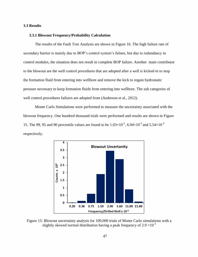
47
3.3 Results
3.3.1 Blowout Frequency/Probability Calculation
The results of the Fault Tree Analysis are shown in Figure 16. The high failure rate of
secondary barrier is mainly due to BOP’s control system’s failure, but due to redundancy in
control modules, the situation does not result in complete BOP failure. Another main contributor
to the blowout are the well control procedures that are adopted after a well is kicked-in to stop
the formation fluid from entering into wellbore and remove the kick to regain hydrostatic
pressure necessary to keep formation fluids from entering into wellbore. The sub categories of
well control procedures failures are adopted from (Anderson et al., 2012).
Monte Carlo Simulations were performed to measure the uncertainty associated with the
blowout frequency. One hundred thousand trials were performed and results are shown in Figure
15. The 99, 95 and 90 percentile values are found to be 1.03×10⁻²
, 6.94×10⁻³
and 5.54×10⁻³
respectively.
Figure 15: Blowout uncertainty analysis for 100,000 trials of Monte Carlo simulations with a
slightly skewed normal distribution having a peak frequency of 2.9 ×10⁻³
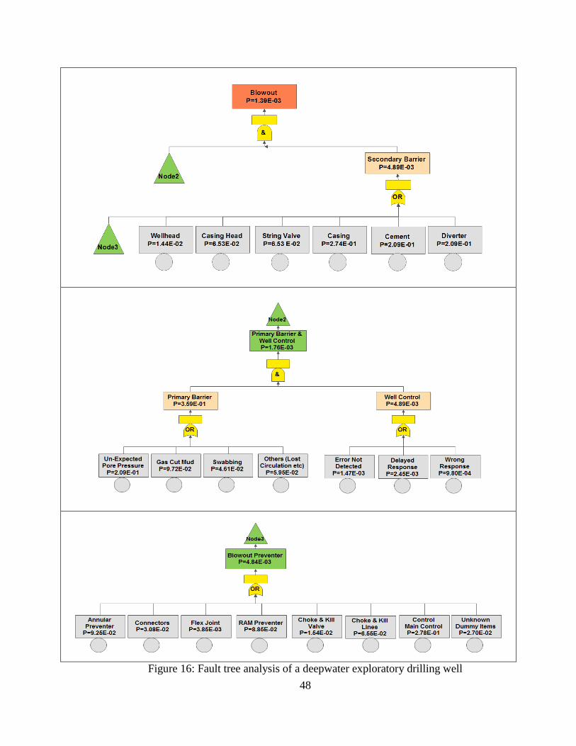
48
Figure 16: Fault tree analysis of a deepwater exploratory drilling well
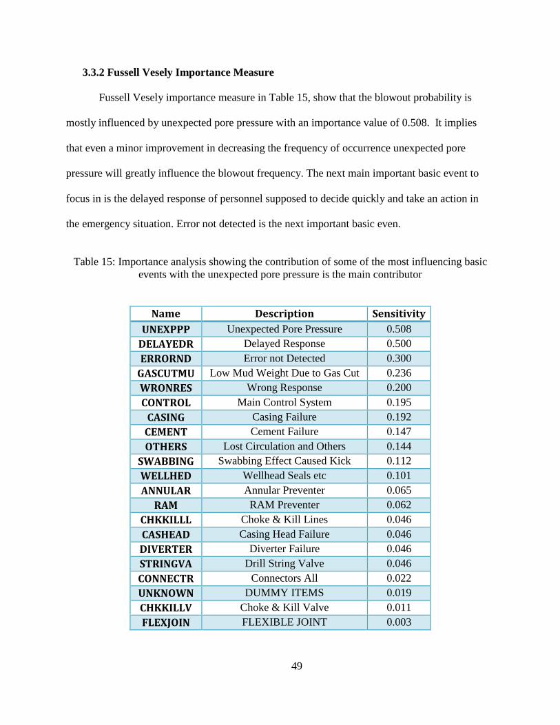
49
3.3.2 Fussell Vesely Importance Measure
Fussell Vesely importance measure in Table 15, show that the blowout probability is
mostly influenced by unexpected pore pressure with an importance value of 0.508. It implies
that even a minor improvement in decreasing the frequency of occurrence unexpected pore
pressure will greatly influence the blowout frequency. The next main important basic event to
focus in is the delayed response of personnel supposed to decide quickly and take an action in
the emergency situation. Error not detected is the next important basic even.
Table 15: Importance analysis showing the contribution of some of the most influencing basic
events with the unexpected pore pressure is the main contributor
Name Description Sensitivity
UNEXPPP Unexpected Pore Pressure 0.508
DELAYEDR Delayed Response 0.500
ERRORND Error not Detected 0.300
GASCUTMU Low Mud Weight Due to Gas Cut 0.236
WRONRES Wrong Response 0.200
CONTROL Main Control System 0.195
CASING Casing Failure 0.192
CEMENT Cement Failure 0.147
OTHERS Lost Circulation and Others 0.144
SWABBING Swabbing Effect Caused Kick 0.112
WELLHED Wellhead Seals etc 0.101
ANNULAR Annular Preventer 0.065
RAM RAM Preventer 0.062
CHKKILLL Choke & Kill Lines 0.046
CASHEAD Casing Head Failure 0.046
DIVERTER Diverter Failure 0.046
STRINGVA Drill String Valve 0.046
CONNECTR Connectors All 0.022
UNKNOWN DUMMY ITEMS 0.019
CHKKILLV Choke & Kill Valve 0.011
FLEXJOIN FLEXIBLE JOINT 0.003
50
This may include the absence/failure of sensors or overlooking some of the potential
early indication of a problem. There is a room to improvement in these areas. Unexpected pore
pressure can be dealt with better seismic profiling and implementing one of the latest drilling
technologies of either wellbore strengthening or drilling with managed pressure. These
techniques will allow better control of bottom hole pressure and allow to drill in well sections
where drilling window is very small. Delay in the response to an event of immediate concern can
be managed with automating some of the initial response decisions and by overseeing the
operations by remotely monitoring the rig activities and take quick decisions and guide the
personnel on the rig floor.
3.3.3 WCD Subsea Release Calculations for P50 Values
A description of the cases modeled in this study is as following. Case numbers are
assigned on the basis of flow path, reservoir penetration and restrictions offered in the flow
paths. While case names are assigned, based on the spill response systems and the time they take
to cap or contain a well and are shown below
RF: Relief Well with duration of 90 days, CS: Capping & Containment System with
effective deployment time of 27 days, CSI: Capping & Containment System with ideal
deployment time of 15 days.
Case ID is the combination of case name and its number. For example for case ID RF1,
RF stands for relief well option for duration calculation and 1 denotes that the fluid is coming
through drill pipe when the reservoir penetration is 5% and BOP is 100% open to flow. The
WCD rates computed, based on the estimated P50 values of reservoir are shown in
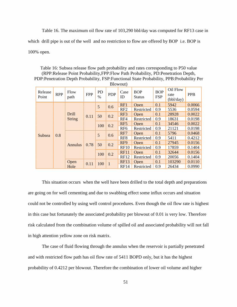
51
Table 16. The maximum oil flow rate of 103,290 bbl/day was computed for RF13 case in
which drill pipe is out of the well and no restriction to flow are offered by BOP i.e. BOP is
100% open.
Table 16: Subsea release flow path probability and rates corresponding to P50 value
(RPP:Release Point Probability,FPP:Flow Path Probability, PD:Penetration Depth,
PDP:Penetration Depth Probability, FSP:Functional State Probability, PPB:Probability Per
Blowout)
Release
Point RPP
Flow
path FPP
PD
% PDP
Case
ID
BOP
Status
BOP
FSP
Oil Flow
rate
(bbl/day)
PPB
Subsea 0.8
Drill
String 0.11
5 0.6 RF1 Open 0.1 5942 0.0066 RF2 Restricted 0.9 5536 0.0594
50 0.2 RF3 Open 0.1 28928 0.0022 RF4 Restricted 0.9 18631 0.0198
100 0.2 RF5 Open 0.1 34546 0.0022 RF6 Restricted 0.9 21121 0.0198
Annulus 0.78
5 0.6 RF7 Open 0.1 5796 0.0468 RF8 Restricted 0.9 5411 0.4212
50 0.2 RF9 Open 0.1 27945 0.0156 RF10 Restricted 0.9 17859 0.1404
100 0.2 RF11 Open 0.1 32644 0.0156 RF12 Restricted 0.9 20056 0.1404
Open
Hole 0.11 100 1
RF13 Open 0.1 103290 0.0110 RF14 Restricted 0.9 26434 0.0990
This situation occurs when the well have been drilled to the total depth and preparations
are going on for well cementing and due to swabbing effect some influx occurs and situation
could not be controlled by using well control procedures. Even though the oil flow rate is highest
in this case but fortunately the associated probability per blowout of 0.01 is very low. Therefore
risk calculated from the combination volume of spilled oil and associated probability will not fall
in high attention yellow zone on risk matrix.
The case of fluid flowing through the annulus when the reservoir is partially penetrated
and with restricted flow path has oil flow rate of 5411 BOPD only, but it has the highest
probability of 0.4212 per blowout. Therefore the combination of lower oil volume and higher
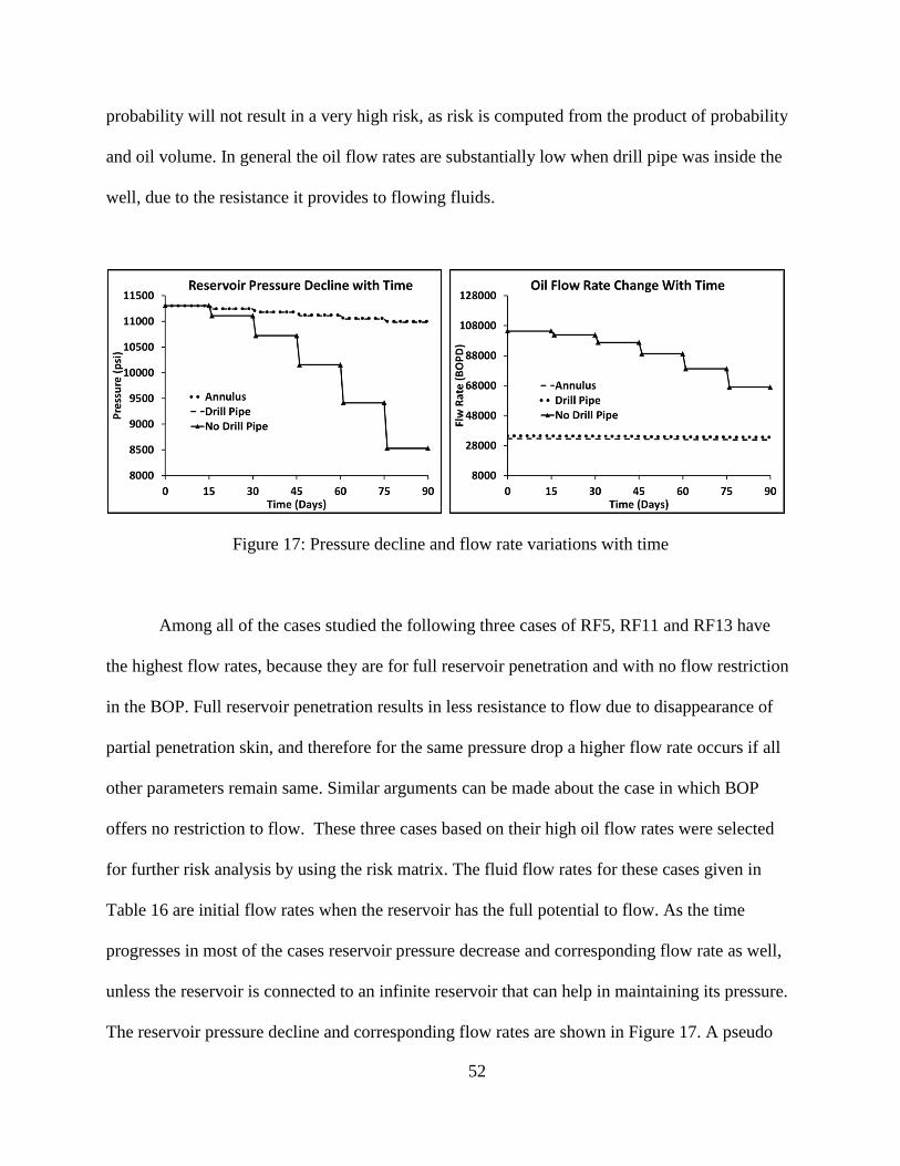
52
probability will not result in a very high risk, as risk is computed from the product of probability
and oil volume. In general the oil flow rates are substantially low when drill pipe was inside the
well, due to the resistance it provides to flowing fluids.
Figure 17: Pressure decline and flow rate variations with time
Among all of the cases studied the following three cases of RF5, RF11 and RF13 have
the highest flow rates, because they are for full reservoir penetration and with no flow restriction
in the BOP. Full reservoir penetration results in less resistance to flow due to disappearance of
partial penetration skin, and therefore for the same pressure drop a higher flow rate occurs if all
other parameters remain same. Similar arguments can be made about the case in which BOP
offers no restriction to flow. These three cases based on their high oil flow rates were selected
for further risk analysis by using the risk matrix. The fluid flow rates for these cases given in
Table 16 are initial flow rates when the reservoir has the full potential to flow. As the time
progresses in most of the cases reservoir pressure decrease and corresponding flow rate as well,
unless the reservoir is connected to an infinite reservoir that can help in maintaining its pressure.
The reservoir pressure decline and corresponding flow rates are shown in Figure 17. A pseudo
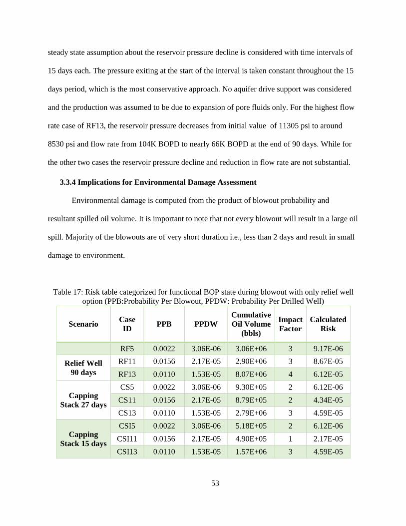
53
steady state assumption about the reservoir pressure decline is considered with time intervals of
15 days each. The pressure exiting at the start of the interval is taken constant throughout the 15
days period, which is the most conservative approach. No aquifer drive support was considered
and the production was assumed to be due to expansion of pore fluids only. For the highest flow
rate case of RF13, the reservoir pressure decreases from initial value of 11305 psi to around
8530 psi and flow rate from 104K BOPD to nearly 66K BOPD at the end of 90 days. While for
the other two cases the reservoir pressure decline and reduction in flow rate are not substantial.
3.3.4 Implications for Environmental Damage Assessment
Environmental damage is computed from the product of blowout probability and
resultant spilled oil volume. It is important to note that not every blowout will result in a large oil
spill. Majority of the blowouts are of very short duration i.e., less than 2 days and result in small
damage to environment.
Table 17: Risk table categorized for functional BOP state during blowout with only relief well
option (PPB:Probability Per Blowout, PPDW: Probability Per Drilled Well)
Scenario Case
ID PPB PPDW
Cumulative
Oil Volume
(bbls)
Impact
Factor
Calculated
Risk
RF5 0.0022 3.06E-06 3.06E+06 3 9.17E-06
Relief Well
90 days
RF11 0.0156 2.17E-05 2.90E+06 3 8.67E-05
RF13 0.0110 1.53E-05 8.07E+06 4 6.12E-05
Capping
Stack 27 days
CS5 0.0022 3.06E-06 9.30E+05 2 6.12E-06
CS11 0.0156 2.17E-05 8.79E+05 2 4.34E-05
CS13 0.0110 1.53E-05 2.79E+06 3 4.59E-05
Capping
Stack 15 days
CSI5 0.0022 3.06E-06 5.18E+05 2 6.12E-06
CSI11 0.0156 2.17E-05 4.90E+05 1 2.17E-05
CSI13 0.0110 1.53E-05 1.57E+06 3 4.59E-05
54
In terms of released oil volume in the past 50 years only 19 spills are reported in the GoM
for all of drilling and production activities that are equal to or greater than 1000 bbl of oil.
Macondo blowout is the biggest outlier with estimated 4.9 million bbl (Anderson et al., 2012) of
oil spilled to environment. The maximum environmental damage is caused when all other efforts
to stop the blowing well are failed and relief well is the only response option left. A time frame
of 90 days duration is considered to drill a relief well for the water and well depths considered in
this scenario.
Please note that duration of relief well drilling may vary depending on the location of the
well, water depth and target zone depth below mud line. In majority of the cases the blowout
may be put under control in a few days’ time frame, either through crew intervention or by the
deployment of spill response systems. The probability of spill having 90 days duration is 0.03
only. The conservative approximate duration estimate for the successful deployment of capping
and containment system is calculated to be 27 days. Ideally these response systems are designed
to cap or contain the blowing well within 15 days’ time frame.
The risk calculations for the base and modified cases are shown in Table 17. The
cumulative volume of oil discharged to the environment is calculated by using the durations for
base and modified cases of 90 and 27 days respectively. The spilled amount estimate is for RF13,
i.e., absolute open flow is around 8.07 million barrels of oil, resulting in impact factor of 4. Due
to their low flow rates, the cases RF5 and RF11 result in impact of 3. With the application of
capping and containment systems the impact factors are substantially reduced.
In the event that the well integrity concerns prohibit the shut in by using capping and
containment systems, these systems have the designed capabilities to collect the hydrocarbons up
to 100,000 BOPD, which is nearly equal to the maximum oil rate calculated. So most probable
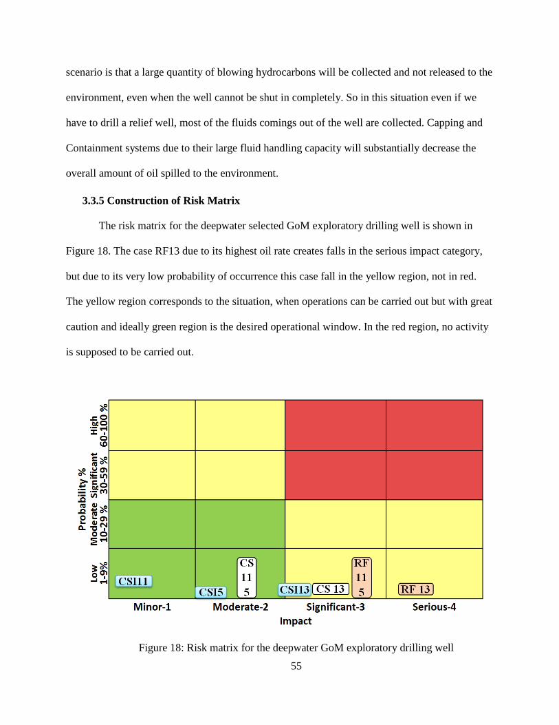
55
scenario is that a large quantity of blowing hydrocarbons will be collected and not released to the
environment, even when the well cannot be shut in completely. So in this situation even if we
have to drill a relief well, most of the fluids comings out of the well are collected. Capping and
Containment systems due to their large fluid handling capacity will substantially decrease the
overall amount of oil spilled to the environment.
3.3.5 Construction of Risk Matrix
The risk matrix for the deepwater selected GoM exploratory drilling well is shown in
Figure 18. The case RF13 due to its highest oil rate creates falls in the serious impact category,
but due to its very low probability of occurrence this case fall in the yellow region, not in red.
The yellow region corresponds to the situation, when operations can be carried out but with great
caution and ideally green region is the desired operational window. In the red region, no activity
is supposed to be carried out.
Figure 18: Risk matrix for the deepwater GoM exploratory drilling well
56
With the deployment of capping and containment response system, the impact category
of this case is reduced from serious-4 to significant-3 and that is a substantial impact reduction.
But still it is in the cautionary yellow zone. If the capping and containment system is
successfully deployed during their designed deployment time frame of 15 days, then the impact
category is further reduced and it moves towards the green region.
The impact factor for other cases of flow through annulus RF11 and through drill pipe
RF5 are also reduced from significant to moderate level when capping and containment system is
available. These results signify the importance of newly built response systems in reducing the
risk of large oil spills.
3.4 Concluding Remarks on Risk Associated With Deepwater Exploratory Well
An example of quantitative risk assessment (QRA) for deepwater exploratory drilling well
blowout is presented, QRA facilitated in better understanding of blowout risks.
The selection of a specific well and corresponding reservoir properties and taking into
account the regional variation in reservoir properties by fitting lognormal/triangular
distributions and conducting Monte Carlo simulations, provided a realistic representation of
the reservoir properties to calculate the worst case discharge rates.
Unexpected pore pressure, delayed response to an incident and failure to detect the error
were found to be three most important basic events contributing to the overall risk of the
system. These were identified by conducting Fussell Vesely (FV) importance analysis.
The FV importance analysis emphasize the need to focus on the technologies to provide
early warnings for unexpected pore pressure during drilling phase, eliminating the delays
57
that can occur when responding to an emergency situation by automation of some of the
decision processes and technologically improve the reliability of sensors that detect an
error. Crew training and management is also an important element in responding to
situations that needs immediate attention.
The worst case discharge rate of nearly 104,000 BOPD was estimated for the case when
drill pipe is out of the hole and BOP offers no restriction to blowing hydrocarbons
(conditions specified by BSEE to estimate WCD). The occurrence of this combination of
events is amongst the least probable situations. Therefore risk which is a product of
probability and spilled oil volume is not very high in this case.
The 100,000 BOPD oil handling capacity of newly built capping and containment systems
is nearly sufficient to either capture or contain the computed worst case discharge oil rate
of 104,000 BPD.
The reservoir pressure drop and resultant reduction in flow rate are not significant in the
cases when the fluids are flowing either through drillpipe-casing annulus or through drill
pipe.
The selection of the multiphase correlation also affects the worst case discharge rate
estimates and computed values with some other correlation may differ from the values
computed in this study, therefore this variation in values must be considered when making
decision based on the WCD rates.
Restrictions in the flow path substantially decrease the fluid flow rate and in some of the
circumstances may even choke the flow.
Newly built response systems are effective in reducing the risk of large oil spill in
deepwaters environments, provided that they function properly when they are deployed.
58
Capping and containment systems are effectives for only one type of failure mode i.e.,
when the flow is coming through the well, which is the most probable scenario based on
the historical blowout data.
Addition of intervention module in capping and containment systems will enhance their
capabilities to deal with other failure modes as well. For example dynamic kill may be used
in the case of an underground blowout.
In the case of a blowing well affecting nearby wells, the situation may become complex
and would require additional modules to be added with capping and containment systems
or invoke other response systems.
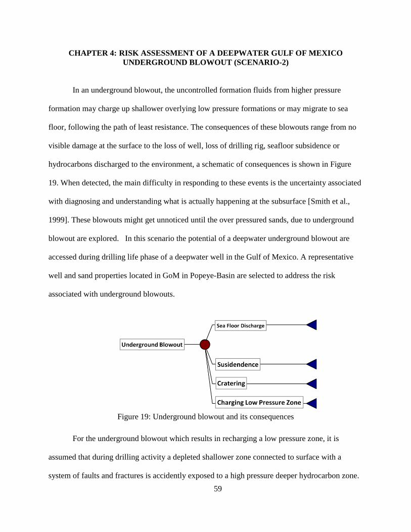
59
CHAPTER 4: RISK ASSESSMENT OF A DEEPWATER GULF OF MEXICO
UNDERGROUND BLOWOUT (SCENARIO-2)
In an underground blowout, the uncontrolled formation fluids from higher pressure
formation may charge up shallower overlying low pressure formations or may migrate to sea
floor, following the path of least resistance. The consequences of these blowouts range from no
visible damage at the surface to the loss of well, loss of drilling rig, seafloor subsidence or
hydrocarbons discharged to the environment, a schematic of consequences is shown in Figure
19. When detected, the main difficulty in responding to these events is the uncertainty associated
with diagnosing and understanding what is actually happening at the subsurface [Smith et al.,
1999]. These blowouts might get unnoticed until the over pressured sands, due to underground
blowout are explored. In this scenario the potential of a deepwater underground blowout are
accessed during drilling life phase of a deepwater well in the Gulf of Mexico. A representative
well and sand properties located in GoM in Popeye-Basin are selected to address the risk
associated with underground blowouts.
Figure 19: Underground blowout and its consequences
For the underground blowout which results in recharging a low pressure zone, it is
assumed that during drilling activity a depleted shallower zone connected to surface with a
system of faults and fractures is accidently exposed to a high pressure deeper hydrocarbon zone.
60
These zones are connected through a conductive fault. The pressure of the deeper zone is high
enough to activate the communicating fault and hydrocarbons migrate to depleted shallower
zone. It is assumed that a system of exiting fractures in the upper zone is activated when its
pressure reaches to the leak of test pressure value. The potential consequences in terms of fluid
discharging to sea floor, subsidence occurrence and the probability of cratering are addressed in
this study. Inside the wellbore, most sensitive point for formation breakdown is the casing shoe,
but it can happen anywhere in the wellbore where formation is the weakest for that particular
wellbore pressure. Due to only partial loss of pressure at the surface; it is difficult to determine if
the underground blowout has occurred.
4.1 Natural Hydrocarbon Seeps in GoM
4.1.1 Geological Features
Complexity of the northern GOM slope geology is a result of interplay of the sediments
(Roberts H. Harry & Carney S. Robert, 1997). Acoustic wipe out zones have been identified, that
are extending from subsurface to seafloor, confirming the evidence that the gas and oil migrated
to the seafloor through these zones. The faults associated with deep salt bodies have greater
potential to act as carrier of hydrocarbons to the sea floor than the faults at the lower depths
above salt domes. It has been reported in the literature that some of the plays in the GoM, have
sands that have pore pressures exceeding the least principle stress of overlying shale seals and
creating new fractures or causing the old one to dilate and allowing fluid migration to upper
layers, that sometimes leads to sea floor venting as well (Seldon, 2005).
4.1.2 Popeye-Genesis Minibasin
It has been reported in the literature that in Popeye-Genesis minibasin in the GoM, fluids
from the reservoirs are venting to sea floor (Seldon, 2005). Due to rapid depositional rate, the
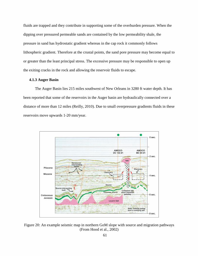
61
fluids are trapped and they contribute in supporting some of the overburden pressure. When the
dipping over pressured permeable sands are contained by the low permeability shale, the
pressure in sand has hydrostatic gradient whereas in the cap rock it commonly follows
lithospheric gradient. Therefore at the crustal points, the sand pore pressure may become equal to
or greater than the least principal stress. The excessive pressure may be responsible to open up
the exiting cracks in the rock and allowing the reservoir fluids to escape.
4.1.3 Auger Basin
The Auger Basin lies 215 miles southwest of New Orleans in 3280 ft water depth. It has
been reported that some of the reservoirs in the Auger basin are hydraulically connected over a
distance of more than 12 miles (Reilly, 2010). Due to small overpressure gradients fluids in these
reservoirs move upwards 1-20 mm/year.
Figure 20: An example seismic map in northern GoM slope with source and migration pathways
(From Hood et al., 2002)
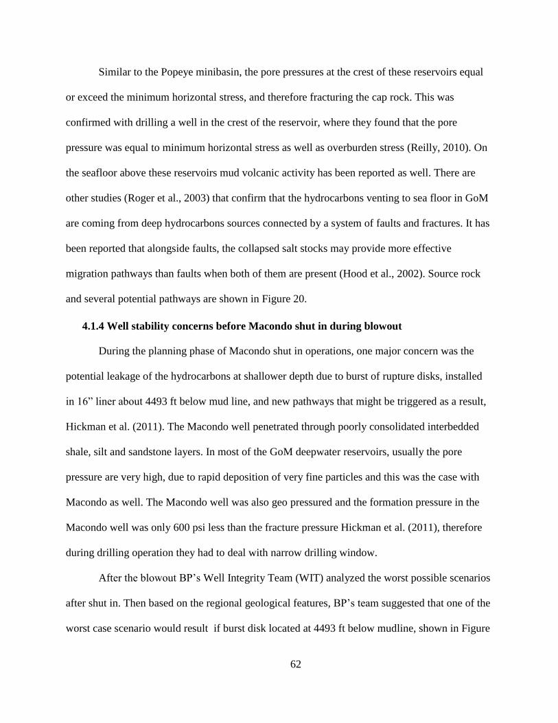
62
Similar to the Popeye minibasin, the pore pressures at the crest of these reservoirs equal
or exceed the minimum horizontal stress, and therefore fracturing the cap rock. This was
confirmed with drilling a well in the crest of the reservoir, where they found that the pore
pressure was equal to minimum horizontal stress as well as overburden stress (Reilly, 2010). On
the seafloor above these reservoirs mud volcanic activity has been reported as well. There are
other studies (Roger et al., 2003) that confirm that the hydrocarbons venting to sea floor in GoM
are coming from deep hydrocarbons sources connected by a system of faults and fractures. It has
been reported that alongside faults, the collapsed salt stocks may provide more effective
migration pathways than faults when both of them are present (Hood et al., 2002). Source rock
and several potential pathways are shown in Figure 20.
4.1.4 Well stability concerns before Macondo shut in during blowout
During the planning phase of Macondo shut in operations, one major concern was the
potential leakage of the hydrocarbons at shallower depth due to burst of rupture disks, installed
in 16” liner about 4493 ft below mud line, and new pathways that might be triggered as a result,
Hickman et al. (2011). The Macondo well penetrated through poorly consolidated interbedded
shale, silt and sandstone layers. In most of the GoM deepwater reservoirs, usually the pore
pressure are very high, due to rapid deposition of very fine particles and this was the case with
Macondo as well. The Macondo well was also geo pressured and the formation pressure in the
Macondo well was only 600 psi less than the fracture pressure Hickman et al. (2011), therefore
during drilling operation they had to deal with narrow drilling window.
After the blowout BP’s Well Integrity Team (WIT) analyzed the worst possible scenarios
after shut in. Then based on the regional geological features, BP’s team suggested that one of the
worst case scenario would result if burst disk located at 4493 ft below mudline, shown in Figure
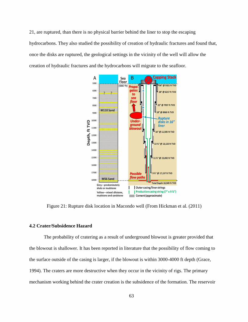
63
21, are ruptured, than there is no physical barrier behind the liner to stop the escaping
hydrocarbons. They also studied the possibility of creation of hydraulic fractures and found that,
once the disks are ruptured, the geological settings in the vicinity of the well will allow the
creation of hydraulic fractures and the hydrocarbons will migrate to the seafloor.
Figure 21: Rupture disk location in Macondo well (From Hickman et al. (2011)
4.2 Crater/Subsidence Hazard
The probability of cratering as a result of underground blowout is greater provided that
the blowout is shallower. It has been reported in literature that the possibility of flow coming to
the surface outside of the casing is larger, if the blowout is within 3000-4000 ft depth (Grace,
1994). The craters are more destructive when they occur in the vicinity of rigs. The primary
mechanism working behind the crater creation is the subsidence of the formation. The reservoir
64
fluid pressure and the rock matrix support the weight of the overlying sediments. In the event of
a shallow underground blowout, the fluid pressure in the producing formation may be reduced
substantially and overburden is now mostly supported by the rock only, and the formation is
compacted. The subsurface compaction may result in the subsidence, depending on the depth and
extent of the reservoir. This type of phenomenon may cause large damage to the surface and
subsurface facilities (Bruno, 1992). The subsidence has been observed during normal production
operations as well.
Case Histories for Crater/Subsidence: Few Examples are presented here to highlight
the potential of crater formation of subsidence.
Drilling Crater Case 1: During drilling a gas well, a large crater thought to be 600 ft
deep, was created in Conroe Oil Field Texas, in 1933 when a gas well blow out caught fire and it
destroyed the rig as well.
Drilling Crater Case 2: A large crater was created in Lake Peigneur in Louisiana that
was nearly 1300 ft deep, the rig was destroyed. It was found later on that the drilling crew
miscalculated their drilling position and drilled through salt dome and into a salt mine deep
under the lake. The impact of the crater was such on a scale that another installation in the lake
docks, another drilling platform, a 70 acre island in the middle of the lake, eleven barges,
vehicles, trees and a parking lot near the lake were all sucked into the mine below. The pull of
the whirlpool was so strong that it reversed the flow of the 12-mile-long Delcambre Canal that
drained the lake into the Gulf of Mexico (Staci Lehman, 2014).
Producing Field Case 1: Wilmington oil filed in California subsided nearly 33 ft during
1935-65 period. This caused casing failures in hundreds of well and raising and repairing the
facilities resulted in cost exceeding more $100 million, till 1962 (Bruno, 1992).
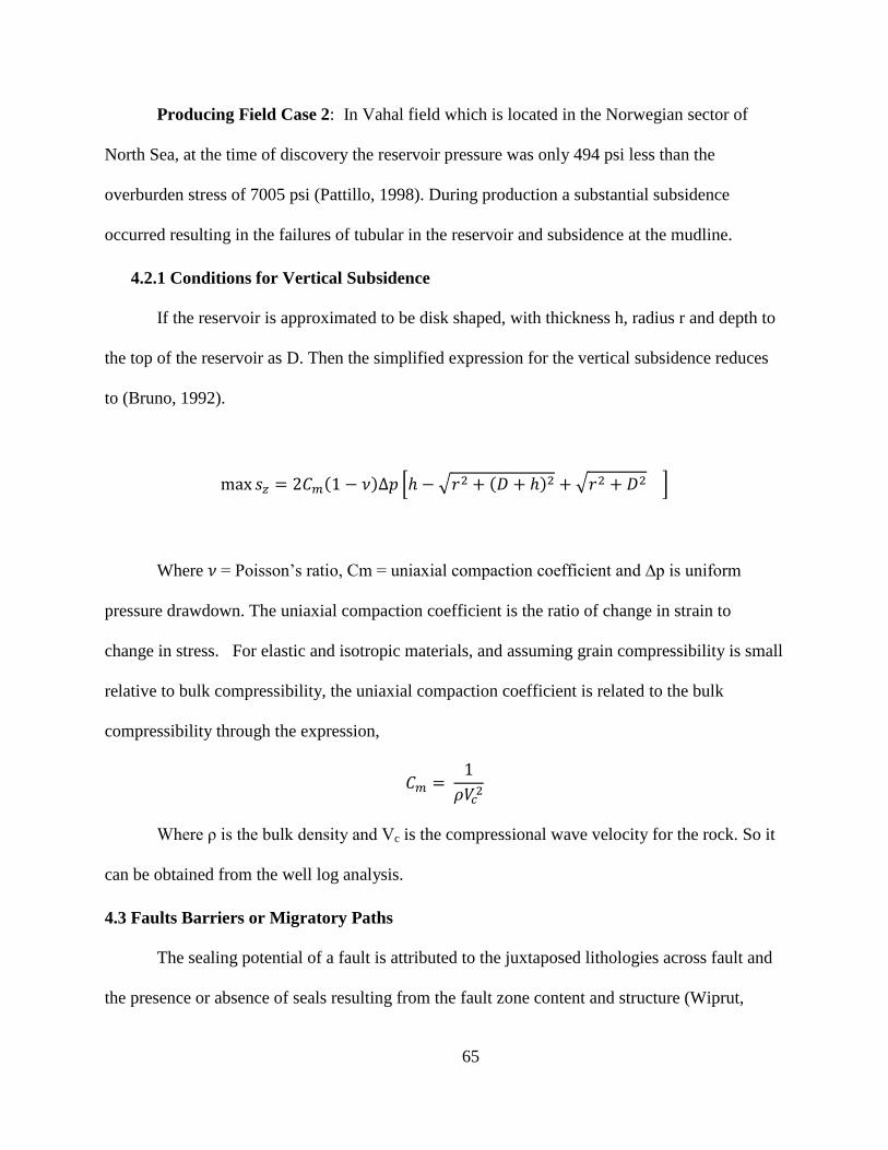
65
Producing Field Case 2: In Vahal field which is located in the Norwegian sector of
North Sea, at the time of discovery the reservoir pressure was only 494 psi less than the
overburden stress of 7005 psi (Pattillo, 1998). During production a substantial subsidence
occurred resulting in the failures of tubular in the reservoir and subsidence at the mudline.
4.2.1 Conditions for Vertical Subsidence
If the reservoir is approximated to be disk shaped, with thickness h, radius r and depth to
the top of the reservoir as D. Then the simplified expression for the vertical subsidence reduces
to (Bruno, 1992).
max 𝑠𝑧 = 2𝐶𝑚(1 − 𝜈)∆𝑝 [ℎ − √𝑟2 + (𝐷 + ℎ)2 + √𝑟2 + 𝐷2 ]
Where 𝜈 = Poisson’s ratio, Cm = uniaxial compaction coefficient and ∆p is uniform
pressure drawdown. The uniaxial compaction coefficient is the ratio of change in strain to
change in stress. For elastic and isotropic materials, and assuming grain compressibility is small
relative to bulk compressibility, the uniaxial compaction coefficient is related to the bulk
compressibility through the expression,
𝐶𝑚 = 1
𝜌𝑉𝑐2
Where ρ is the bulk density and Vc is the compressional wave velocity for the rock. So it
can be obtained from the well log analysis.
4.3 Faults Barriers or Migratory Paths
The sealing potential of a fault is attributed to the juxtaposed lithologies across fault and
the presence or absence of seals resulting from the fault zone content and structure (Wiprut,
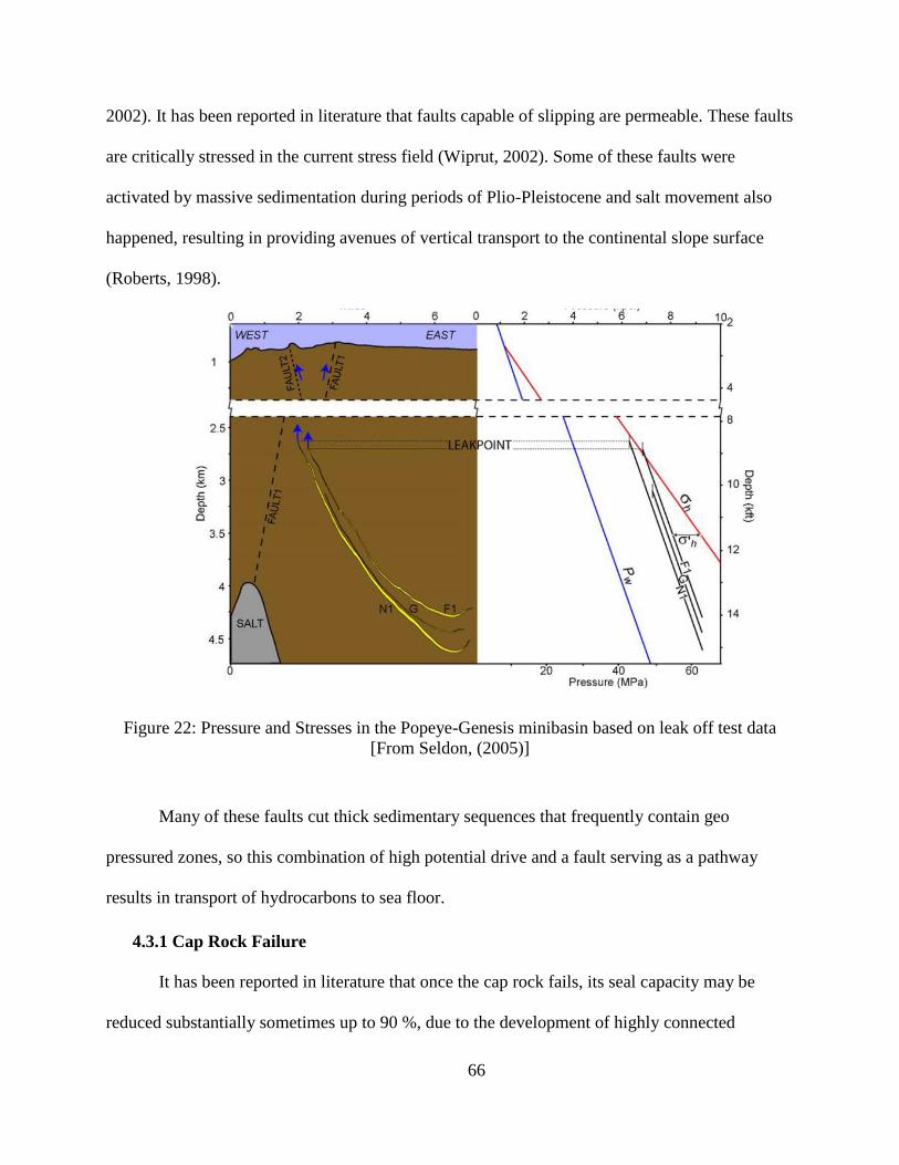
66
2002). It has been reported in literature that faults capable of slipping are permeable. These faults
are critically stressed in the current stress field (Wiprut, 2002). Some of these faults were
activated by massive sedimentation during periods of Plio-Pleistocene and salt movement also
happened, resulting in providing avenues of vertical transport to the continental slope surface
(Roberts, 1998).
Figure 22: Pressure and Stresses in the Popeye-Genesis minibasin based on leak off test data
[From Seldon, (2005)]
Many of these faults cut thick sedimentary sequences that frequently contain geo
pressured zones, so this combination of high potential drive and a fault serving as a pathway
results in transport of hydrocarbons to sea floor.
4.3.1 Cap Rock Failure
It has been reported in literature that once the cap rock fails, its seal capacity may be
reduced substantially sometimes up to 90 %, due to the development of highly connected
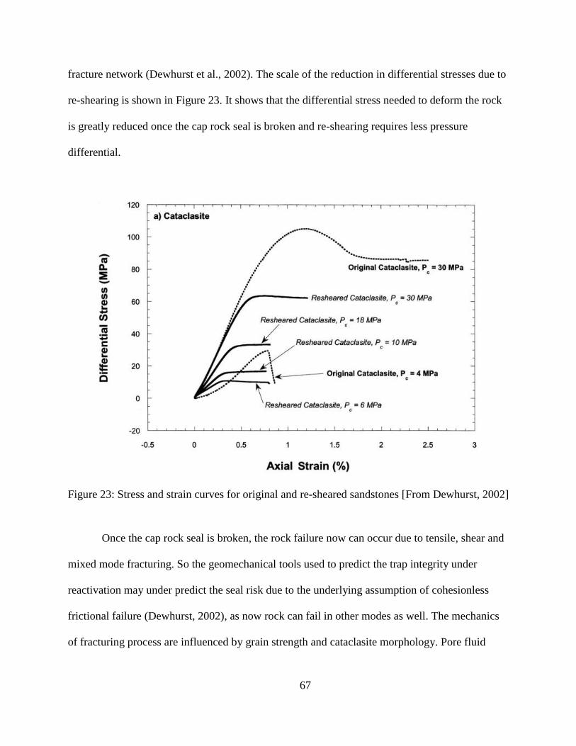
67
fracture network (Dewhurst et al., 2002). The scale of the reduction in differential stresses due to
re-shearing is shown in Figure 23. It shows that the differential stress needed to deform the rock
is greatly reduced once the cap rock seal is broken and re-shearing requires less pressure
differential.
Figure 23: Stress and strain curves for original and re-sheared sandstones [From Dewhurst, 2002]
Once the cap rock seal is broken, the rock failure now can occur due to tensile, shear and
mixed mode fracturing. So the geomechanical tools used to predict the trap integrity under
reactivation may under predict the seal risk due to the underlying assumption of cohesionless
frictional failure (Dewhurst, 2002), as now rock can fail in other modes as well. The mechanics
of fracturing process are influenced by grain strength and cataclasite morphology. Pore fluid
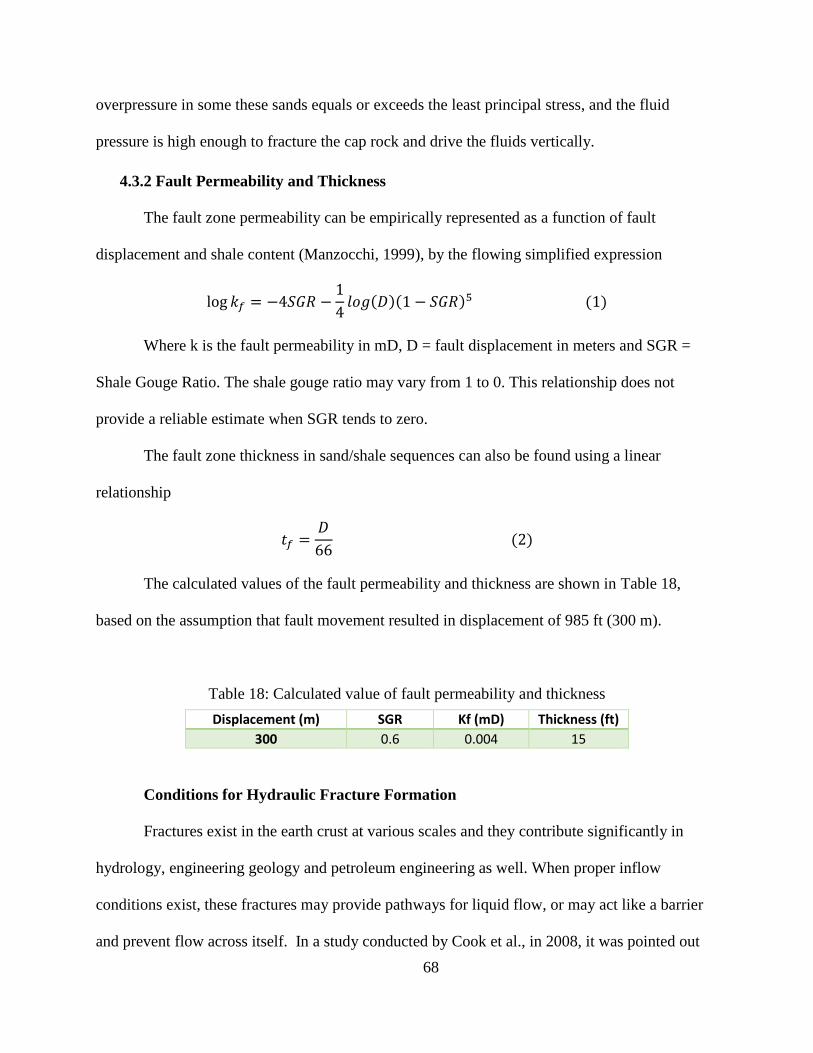
68
overpressure in some these sands equals or exceeds the least principal stress, and the fluid
pressure is high enough to fracture the cap rock and drive the fluids vertically.
4.3.2 Fault Permeability and Thickness
The fault zone permeability can be empirically represented as a function of fault
displacement and shale content (Manzocchi, 1999), by the flowing simplified expression
log 𝑘𝑓 = −4𝑆𝐺𝑅 −1
4𝑙𝑜𝑔(𝐷)(1 − 𝑆𝐺𝑅)5 (1)
Where k is the fault permeability in mD, D = fault displacement in meters and SGR =
Shale Gouge Ratio. The shale gouge ratio may vary from 1 to 0. This relationship does not
provide a reliable estimate when SGR tends to zero.
The fault zone thickness in sand/shale sequences can also be found using a linear
relationship
𝑡𝑓 =𝐷
66 (2)
The calculated values of the fault permeability and thickness are shown in Table 18,
based on the assumption that fault movement resulted in displacement of 985 ft (300 m).
Table 18: Calculated value of fault permeability and thickness
Displacement (m) SGR Kf (mD) Thickness (ft)
300 0.6 0.004 15
Conditions for Hydraulic Fracture Formation
Fractures exist in the earth crust at various scales and they contribute significantly in
hydrology, engineering geology and petroleum engineering as well. When proper inflow
conditions exist, these fractures may provide pathways for liquid flow, or may act like a barrier
and prevent flow across itself. In a study conducted by Cook et al., in 2008, it was pointed out
69
that natural gas hydrates present in Keathley Canyon in GoM were controlled by presence of
natural fractures. Natural oil and gas seeps are present in the Gulf of Mexico and other petroleum
prolific regions of the world (Reilly et al., 2010).
Stresses and Fracture opening and propagation
In the porous media, the weight of the overburden is carried by both the grains and the
pore fluid. Therefore, an effective stress, 𝜎𝑣′ is defined as
𝜎𝑣′ = 𝜎𝑣 − 𝛼𝑝
Where 𝜎𝑣 = overburden stress, p = pore pressure, α = Biot’s poroelastic coefficient
(ranges from 0 to 1)
Horizontal and vertical stresses are related through Poisson’s ratio 𝜈
𝜎𝐻′ = (
𝜐
1 − 𝜐) 𝜎𝑣
′
Due to the presence of tectonic forces, the horizontal stress varies with direction, and
horizontal stresses can be related by
𝜎𝐻,𝑚𝑎𝑥 = 𝜎𝐻,𝑚𝑖𝑛 + 𝜎𝑡𝑒𝑐𝑡𝑜𝑛𝑖𝑐
Usually the overburden stress is the largest amongst the three principal stresses and these
can be expressed as
𝜎𝑣 ≥ 𝜎𝐻 𝑚𝑎𝑥 ≥ 𝜎𝐻 𝑚𝑖𝑛
The minimum horizontal stress can be found by the leakoff test, mini frac test and
theoretically by using the following poroelasticity equation
Pressure to Fracture a Formation: The breakdown pressure required for a non-
penetrating fluid to fracture a formation for a vertical well is taken from work Hamison (1967).
70
𝑝𝑏𝑑 𝑛𝑝 = 3𝜎𝐻 𝑚𝑖𝑛 − 𝜎𝐻,𝑚𝑖𝑛 + 𝑇𝑜 − 𝑝
where
Pbd,np = breakdown pressure for non-penetrating fluid
To = tensile strength of rock
P = reservoir pressure
The breakdown pressure for penetrating fluid is less than the pressure required for non-
penetrating fluid and is given by
𝑝𝑏𝑑 𝑝𝑒𝑛𝑒𝑡𝑟𝑎𝑡𝑖𝑛𝑔 =3𝜎𝐻 𝑚𝑖𝑛 − 𝜎𝐻,𝑚𝑖𝑛 + 𝑇𝑜 − 2𝜂𝑝
2(1 − 𝜂)
where
𝜂 = 𝛼 (1 − 2𝜐)
2(1 − 𝜐)
The pressure required to propagate the fracture is usually less than the breakdown
pressure.
Fracture Permeability: Once fractures are created they can conduct at much higher rates
than the reservoir sands. The ratio of fracture permeability to matrix permeability is an important
parameter to consider when analyzing the fluid conductance through fractures. The fracture
permeability contribution and ranges have been categorized by Matthai (2003), as following
1. For 𝑘𝑓
𝑘𝑣⁄ = 102 fracture do not contribute significantly to the effective permeability of
the reservoir.
2. For 𝑘𝑓
𝑘𝑣⁄ = 103 − 104 a transition occurs and the fracture start contributing to the
effective permeability of the reservoir.
71
3. For 𝑘𝑓
𝑘𝑣⁄ = 105 − 106 main flow is carried by the well connected fractures and
contribution of fracture permeability to the effective permeability of the reservoir becomes
significant.
Similar arguments can be made about the systems of faults connecting a high pressure deeper
zone to a lower pressure shallower zone. If the permeability of this conductive zone is above a
threshold value, than it can considerably conduct substantial hydrocarbons in short amount of
time, otherwise it may take centuries to overcharge the shallower low pressure zone.
Flow through Fracture: Fluid flow through fractures is usually modeled by the using
the concept of two parallel plates. With the assumptions of laminar, incompressible fluid and
smooth parallel plates, the Navier-Stokes equation reduces to commonly known cubic law for
fracture flow. In reality most of the time, the natural fractures have rough walls and with walls
coming to contact each other at some discrete points and reducing the amount of fluid moving
through them (Klimczak, 2010). Therefore a model incorporating the roughness of walls and the
crookedness of fluid path may be more representative of the true fluid flow in fractures.
4.4 Reservoir Simulation Setup Flow through Faulted Zone
The simulation model used for the analysis is shown below in Figure 24. It is a layered
reservoir, divided into 15 layers. The bottom layer represents the source reservoir and the top
most layer is the shallower low pressure zone. The intermediate layers have a fault that connects
these two zones. An assumption is made that for intermediate layers only faulted region is
conductive and fluid migrate through it to depleted top zone. The top most layer or low pressure
zone has a set of faults and fracture that can transmit the fluids to the sea floor, provided that the
necessary conditions of pressure are met to open up the fractures or reactivation of faults. These
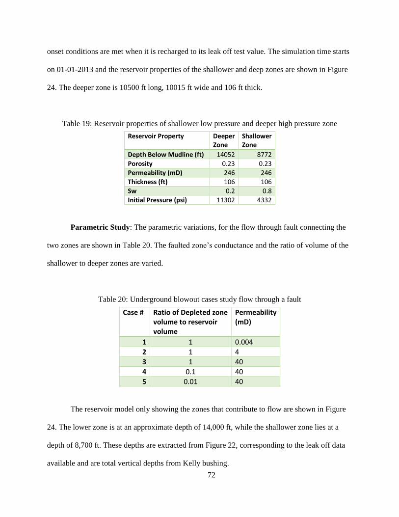
72
onset conditions are met when it is recharged to its leak off test value. The simulation time starts
on 01-01-2013 and the reservoir properties of the shallower and deep zones are shown in Figure
24. The deeper zone is 10500 ft long, 10015 ft wide and 106 ft thick.
Table 19: Reservoir properties of shallower low pressure and deeper high pressure zone
Reservoir Property Deeper Zone
Shallower Zone
Depth Below Mudline (ft) 14052 8772
Porosity 0.23 0.23
Permeability (mD) 246 246
Thickness (ft) 106 106
Sw 0.2 0.8
Initial Pressure (psi) 11302 4332
Parametric Study: The parametric variations, for the flow through fault connecting the
two zones are shown in Table 20. The faulted zone’s conductance and the ratio of volume of the
shallower to deeper zones are varied.
Table 20: Underground blowout cases study flow through a fault
Case # Ratio of Depleted zone volume to reservoir volume
Permeability (mD)
1 1 0.004
2 1 4
3 1 40
4 0.1 40
5 0.01 40
The reservoir model only showing the zones that contribute to flow are shown in Figure
24. The lower zone is at an approximate depth of 14,000 ft, while the shallower zone lies at a
depth of 8,700 ft. These depths are extracted from Figure 22, corresponding to the leak off data
available and are total vertical depths from Kelly bushing.
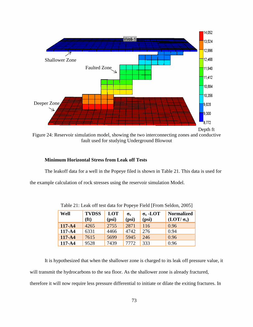
73
Figure 24: Reservoir simulation model, showing the two interconnecting zones and conductive
fault used for studying Underground Blowout
Minimum Horizontal Stress from Leak off Tests
The leakoff data for a well in the Popeye filed is shown in Table 21. This data is used for
the example calculation of rock stresses using the reservoir simulation Model.
Table 21: Leak off test data for Popeye Field [From Seldon, 2005]
Well TVDSS
(ft)
LOT
(psi)
σv
(psi)
σv -LOT
(psi)
Normalized
(LOT/ σv)
117-A4 4265 2755 2871 116 0.96 117-A4 6331 4466 4742 276 0.94
117-A4 7615 5699 5945 246 0.96
117-A4 9528 7439 7772 333 0.96
It is hypothesized that when the shallower zone is charged to its leak off pressure value, it
will transmit the hydrocarbons to the sea floor. As the shallower zone is already fractured,
therefore it will now require less pressure differential to initiate or dilate the exiting fractures. In
Deeper Zone
Depth ft
Faulted Zone
Shallower Zone
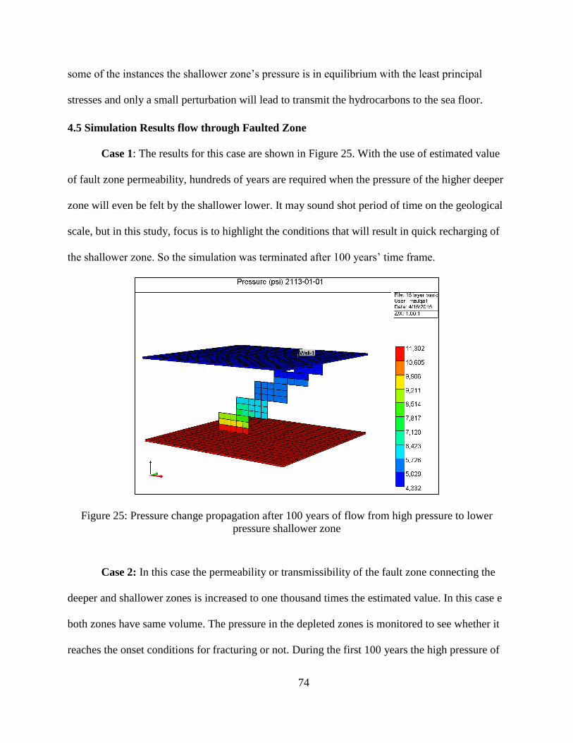
74
some of the instances the shallower zone’s pressure is in equilibrium with the least principal
stresses and only a small perturbation will lead to transmit the hydrocarbons to the sea floor.
4.5 Simulation Results flow through Faulted Zone
Case 1: The results for this case are shown in Figure 25. With the use of estimated value
of fault zone permeability, hundreds of years are required when the pressure of the higher deeper
zone will even be felt by the shallower lower. It may sound shot period of time on the geological
scale, but in this study, focus is to highlight the conditions that will result in quick recharging of
the shallower zone. So the simulation was terminated after 100 years’ time frame.
Figure 25: Pressure change propagation after 100 years of flow from high pressure to lower
pressure shallower zone
Case 2: In this case the permeability or transmissibility of the fault zone connecting the
deeper and shallower zones is increased to one thousand times the estimated value. In this case e
both zones have same volume. The pressure in the depleted zones is monitored to see whether it
reaches the onset conditions for fracturing or not. During the first 100 years the high pressure of
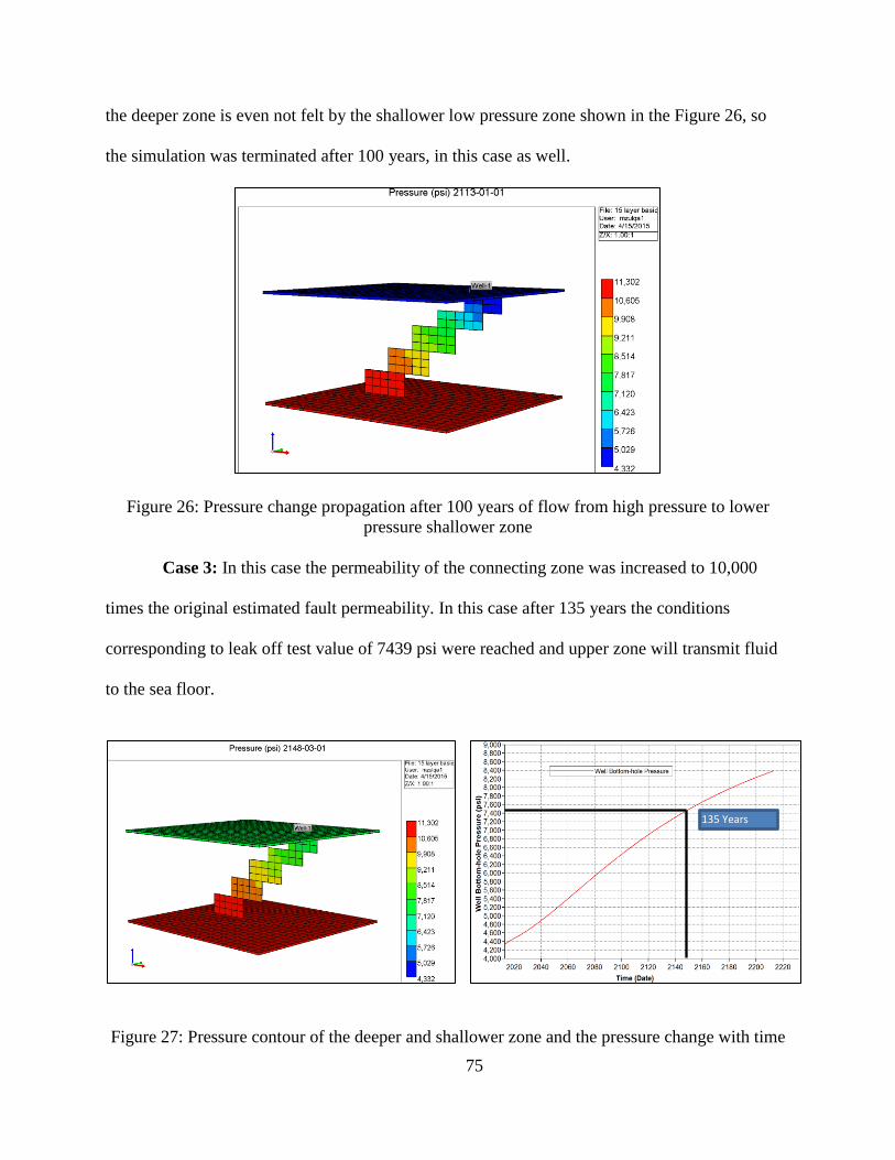
75
the deeper zone is even not felt by the shallower low pressure zone shown in the Figure 26, so
the simulation was terminated after 100 years, in this case as well.
Figure 26: Pressure change propagation after 100 years of flow from high pressure to lower
pressure shallower zone
Case 3: In this case the permeability of the connecting zone was increased to 10,000
times the original estimated fault permeability. In this case after 135 years the conditions
corresponding to leak off test value of 7439 psi were reached and upper zone will transmit fluid
to the sea floor.
Figure 27: Pressure contour of the deeper and shallower zone and the pressure change with time
135 Years
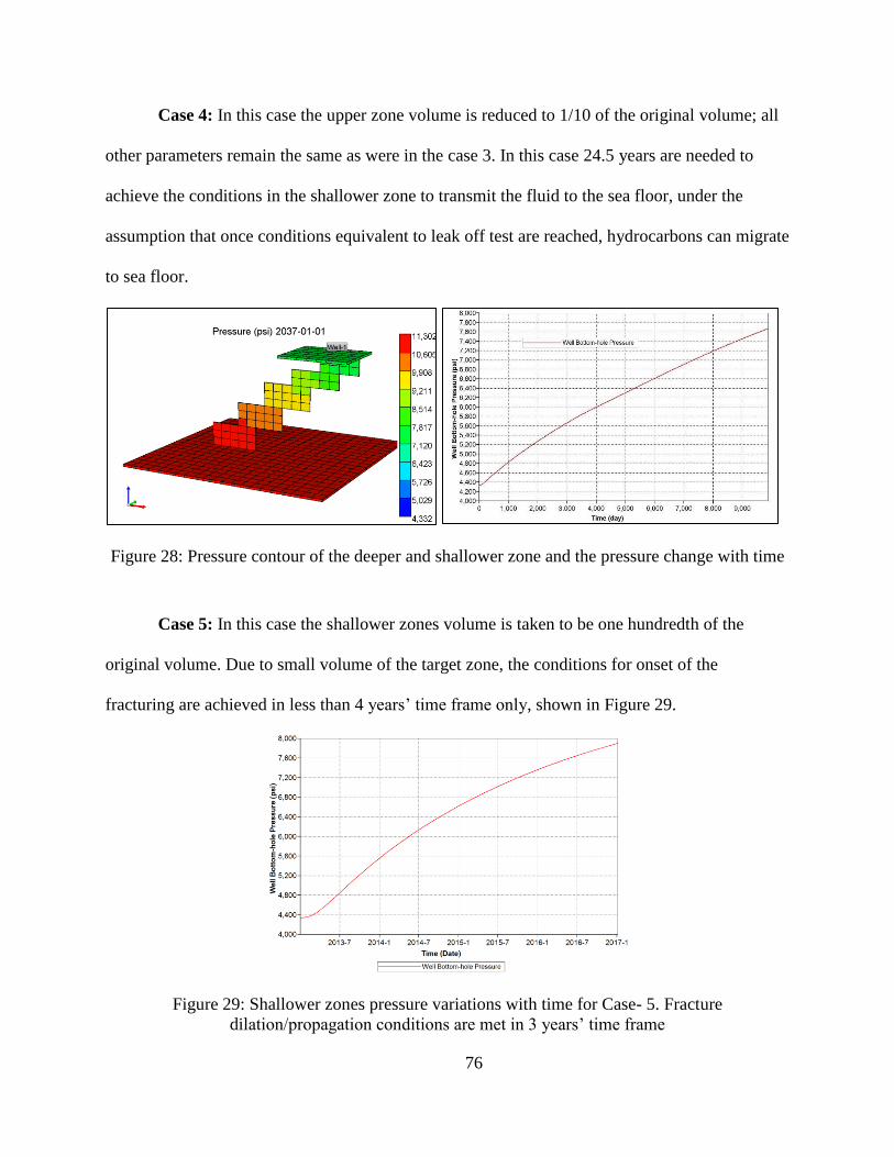
76
Case 4: In this case the upper zone volume is reduced to 1/10 of the original volume; all
other parameters remain the same as were in the case 3. In this case 24.5 years are needed to
achieve the conditions in the shallower zone to transmit the fluid to the sea floor, under the
assumption that once conditions equivalent to leak off test are reached, hydrocarbons can migrate
to sea floor.
Figure 28: Pressure contour of the deeper and shallower zone and the pressure change with time
Case 5: In this case the shallower zones volume is taken to be one hundredth of the
original volume. Due to small volume of the target zone, the conditions for onset of the
fracturing are achieved in less than 4 years’ time frame only, shown in Figure 29.
Figure 29: Shallower zones pressure variations with time for Case- 5. Fracture
dilation/propagation conditions are met in 3 years’ time frame
77
4.6 Observations & Conclusions
The consequences of an underground blowout range from no visible damage at the sea
surface to the loss of the whole rig. It is difficult to quantitatively estimate the risk due to
the involvement of large number of uncertain parameters.
The potential of hydrocarbons leaking to sea floor is a combination of geological settings,
the transmissibility of the paths allowing hydrocarbons to reach sea floor, the pressure of
source reservoir and its potential to create fractures in the low lying geological barriers.
The formulas used to estimate the fault permeability and thickness are very simple and
uncertainty exits in the estimated parameters of fault permeability and its thickness.
The simulation results show that for low permeability k=0.004 mD fault connecting a deep
over pressured zone to a shallower low pressure zone, the time taken to recharge the
shallower zone to reach its LOT pressure value is more than 100 years.
A high permeable faulted zone of 40 mD will take 135 years to recharge the low pressure
shallower zone to its LOT pressure value.
In the reservoir model adopted in this scenario, when the ratio of the volume of shallower
to deeper zone decrease to 0.1, the recharging time significantly drops to 24 years only.
Therefore ratio of the two zones is also an important parameter alongside their pressure
differential and the transmissibility of the connecting zone.
The worst conditions may occur when the hydrocarbons travel through the casing-wellbore
annulus and may either reach to shallowest zones lying very close to mud line or leak
outside of the well. The casing-wellbore annulus path may have very high permeability due
to fractured cement and/or due to micro annulus gaps in this path. In this case the
hydrocarbons may appear at the sea floor during the drilling activity.
78
CHAPTER 5: OIL SPILL RISK ASSESSMENT OF A SAND CONTROL ELEMENT
FAILURE LEADING TO BLOWOUT DURING NORMAL PRODUCTION
OPERATIONS (SCENARIO-3)
A great effort is under way after Macondo incident to improve the safety of deepwater
drilling and production operations and enhance the capabilities of different well barrier to stop
the oil spill on its earliest stages. This study is a part of that collective effort to make offshore
operations safer and decrease the associated risks. The main objective of modeling this scenario
was to investigate the oil spill risk associated with a representative production well in the Gulf of
Mexico during its normal production operations. Identification of most critical elements
contribution to risk assessment in a subsea production well was also among the objectives.
Quantified risk is computed from the product of blowout and volume of oil released to the
environment as a result. Blowout frequency is computed from Fault Tree Analysis (FTA) and
spilled oil volume is estimated from simulating multiphase fluid flow and heat transfer in
wellbores.
Most of the oil wells are completed with some sort of bottom hole sand control elements
to prevent production of sand, when hydrocarbons are produced. The failure of these control
elements may have severe consequence and in some cases may result in uncontrolled
hydrocarbon flowing to the environment. A representative production well from the Mississippi
Canyon in the Gulf of Mexico is selected for the for quantitative risk assessment (QRA) analysis.
The well is completed with cased hole gravel pack and with sand control elements in place. The
representative reservoir properties for this well are selected from the literature and variations in
properties are accounted for by fitting lognormal distribution. Monte Carlo simulations were
performed to find distribution of productivity index. P50 value for the reservoir properties
distributions and PI from Monte Carlo simulation was used to find worst case discharge rates by
79
using a commercially available multiphase flow simulators OLGA and PIPESIM with black oil
fluid model.
A Fault Tree is constructed using LOGAN fault tree analysis software, to find the
blowout probability based on the primary and secondary barrier failure data. From the minimal
cut set method the importance and sensitivity of different well barrier is analyzed and most
critical well barriers are identified.
5.1 Introduction
Quantitative risk assessment provides means to conduct systematic analysis of risk due
to hazard activities and evaluation of various risks reducing measure (Spouge, 1999). Risk to an
offshore installation may be expressed into the main categories of risks posed to human life,
assets, production delay and environment. These are sometimes called “dimensions of risk”
(Vinnem, 2007). Environmental risk/damage is analyzed in this study in the form of amount of
hydrocarbons released to the environment.
Well Barriers: In order to prevent a blowout, the well must be equipped with pressure
control equipment and barriers. As regulatory requirement in all well operations, two tested and
independent well barriers should be in place at all times for abnormally pressured formations
with flow potential NORSOK Standard (2013). Each barrier in itself is intended to prevent
uncontrolled flow of the reservoir fluid to the surroundings. In the production life phase of an
offshore well, the primary barriers are production tubing, SCSSV and production packer, while
the main secondary barriers are Subsea production Tree, wellhead, tubing hanger, casing and
cement behind the casing, these are shown in Figure 30, below. A blowout can only occur when
both of these barriers fails simultaneously.
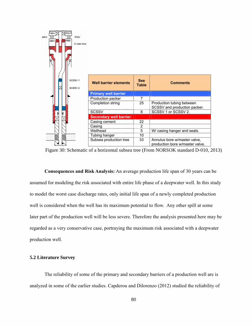
80
Figure 30: Schematic of a horizontal subsea tree (From NORSOK standard D-010, 2013)
Consequences and Risk Analysis: An average production life span of 30 years can be
assumed for modeling the risk associated with entire life phase of a deepwater well. In this study
to model the worst case discharge rates, only initial life span of a newly completed production
well is considered when the well has its maximum potential to flow. Any other spill at some
later part of the production well will be less severe. Therefore the analysis presented here may be
regarded as a very conservative case, portraying the maximum risk associated with a deepwater
production well.
5.2 Literature Survey
The reliability of some of the primary and secondary barriers of a production well are is
analyzed in some of the earlier studies. Capderou and Dilorenzo (2012) studied the reliability of
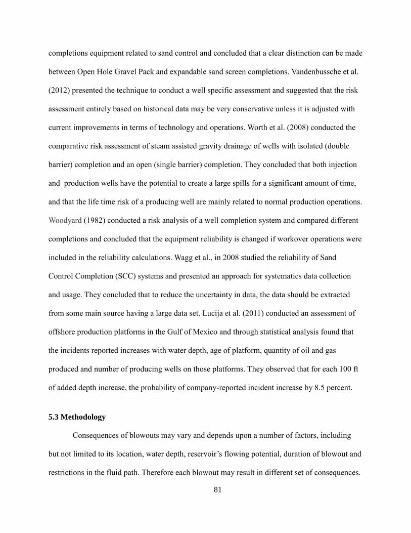
81
completions equipment related to sand control and concluded that a clear distinction can be made
between Open Hole Gravel Pack and expandable sand screen completions. Vandenbussche et al.
(2012) presented the technique to conduct a well specific assessment and suggested that the risk
assessment entirely based on historical data may be very conservative unless it is adjusted with
current improvements in terms of technology and operations. Worth et al. (2008) conducted the
comparative risk assessment of steam assisted gravity drainage of wells with isolated (double
barrier) completion and an open (single barrier) completion. They concluded that both injection
and production wells have the potential to create a large spills for a significant amount of time,
and that the life time risk of a producing well are mainly related to normal production operations.
Woodyard (1982) conducted a risk analysis of a well completion system and compared different
completions and concluded that the equipment reliability is changed if workover operations were
included in the reliability calculations. Wagg et al., in 2008 studied the reliability of Sand
Control Completion (SCC) systems and presented an approach for systematics data collection
and usage. They concluded that to reduce the uncertainty in data, the data should be extracted
from some main source having a large data set. Lucija et al. (2011) conducted an assessment of
offshore production platforms in the Gulf of Mexico and through statistical analysis found that
the incidents reported increases with water depth, age of platform, quantity of oil and gas
produced and number of producing wells on those platforms. They observed that for each 100 ft
of added depth increase, the probability of company-reported incident increase by 8.5 percent.
5.3 Methodology
Consequences of blowouts may vary and depends upon a number of factors, including
but not limited to its location, water depth, reservoir’s flowing potential, duration of blowout and
restrictions in the fluid path. Therefore each blowout may result in different set of consequences.
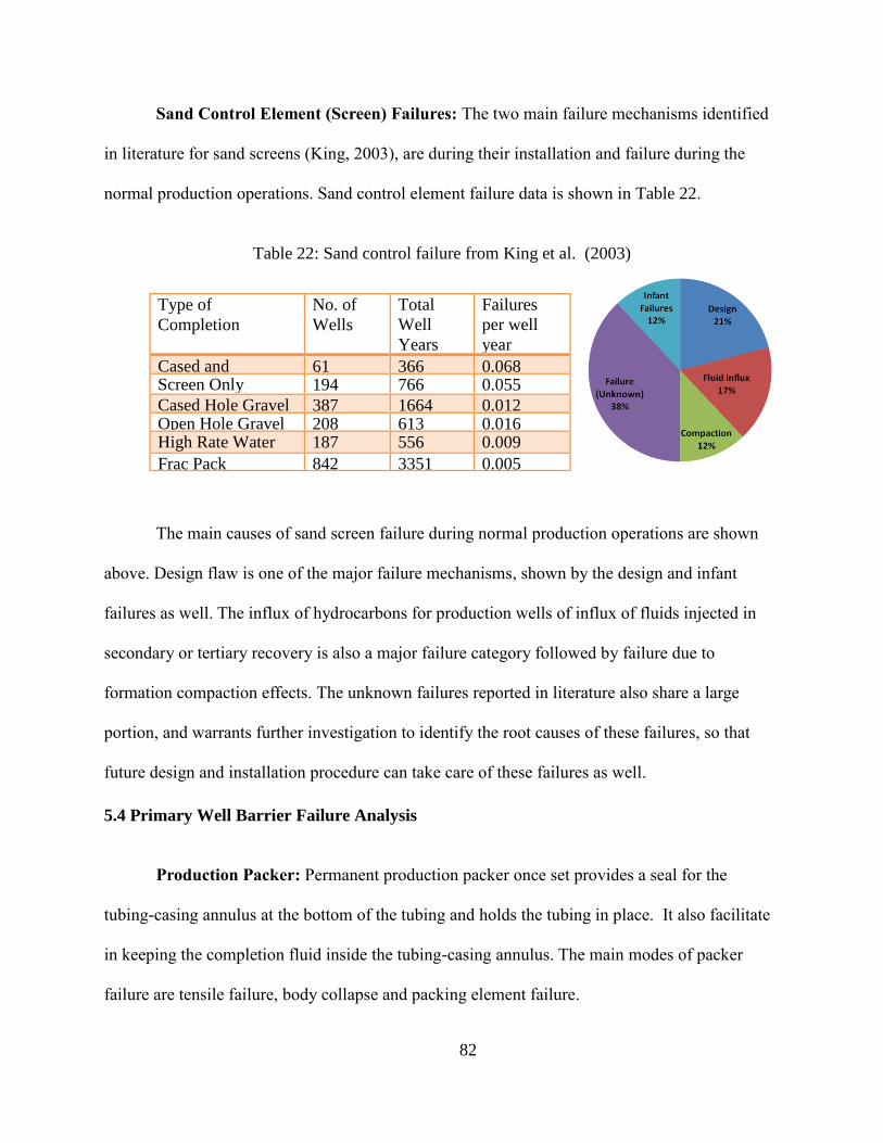
82
Sand Control Element (Screen) Failures: The two main failure mechanisms identified
in literature for sand screens (King, 2003), are during their installation and failure during the
normal production operations. Sand control element failure data is shown in Table 22.
Table 22: Sand control failure from King et al. (2003)
Type of
Completion
No. of
Wells
Total
Well
Years
Failures
per well
year
Cased and
Perforated
61 366 0.068 Screen Only
Completion
194 766 0.055
Cased Hole Gravel
Pack
387 1664 0.012 Open Hole Gravel
Pack
208 613 0.016 High Rate Water
Packs
187 556 0.009
Frac Pack 842 3351 0.005
The main causes of sand screen failure during normal production operations are shown
above. Design flaw is one of the major failure mechanisms, shown by the design and infant
failures as well. The influx of hydrocarbons for production wells of influx of fluids injected in
secondary or tertiary recovery is also a major failure category followed by failure due to
formation compaction effects. The unknown failures reported in literature also share a large
portion, and warrants further investigation to identify the root causes of these failures, so that
future design and installation procedure can take care of these failures as well.
5.4 Primary Well Barrier Failure Analysis
Production Packer: Permanent production packer once set provides a seal for the
tubing-casing annulus at the bottom of the tubing and holds the tubing in place. It also facilitate
in keeping the completion fluid inside the tubing-casing annulus. The main modes of packer
failure are tensile failure, body collapse and packing element failure.
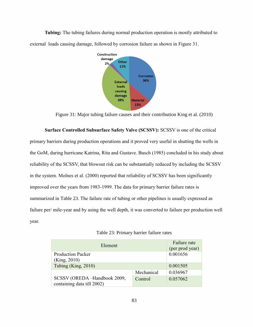
83
Tubing: The tubing failures during normal production operation is mostly attributed to
external loads causing damage, followed by corrosion failure as shown in Figure 31.
Figure 31: Major tubing failure causes and their contribution King et al. (2010)
Surface Controlled Subsurface Safety Valve (SCSSV): SCSSV is one of the critical
primary barriers during production operations and it proved very useful in shutting the wells in
the GoM, during hurricane Katrina, Rita and Gustave. Busch (1985) concluded in his study about
reliability of the SCSSV, that blowout risk can be substantially reduced by including the SCSSV
in the system. Molnes et al. (2000) reported that reliability of SCSSV has been significantly
improved over the years from 1983-1999. The data for primary barrier failure rates is
summarized in Table 23. The failure rate of tubing or other pipelines is usually expressed as
failure per/ mile-year and by using the well depth, it was converted to failure per production well
year.
Table 23: Primary barrier failure rates
Element Failure rate
(per prod year)
Production Packer
(King, 2010)
0.001656
Tubing (King, 2010) 0.001505
SCSSV (OREDA –Handbook 2009,
containing data till 2002)
Mechanical 0.036967
Control 0.057062
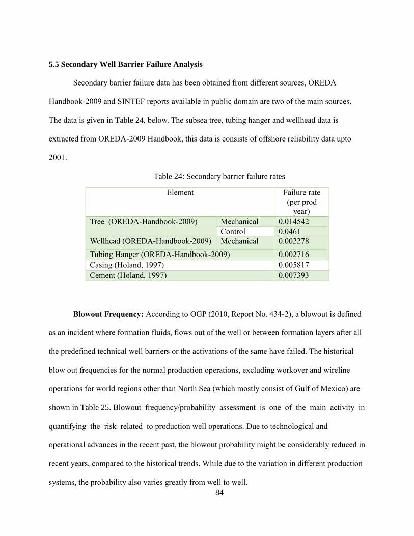
84
5.5 Secondary Well Barrier Failure Analysis
Secondary barrier failure data has been obtained from different sources, OREDA
Handbook-2009 and SINTEF reports available in public domain are two of the main sources.
The data is given in Table 24, below. The subsea tree, tubing hanger and wellhead data is
extracted from OREDA-2009 Handbook, this data is consists of offshore reliability data upto
2001.
Table 24: Secondary barrier failure rates
Element Failure rate
(per prod
year)
Tree (OREDA-Handbook-2009) Mechanical 0.014542
Control 0.0461
Wellhead (OREDA-Handbook-2009) Mechanical 0.002278
Tubing Hanger (OREDA-Handbook-2009) 0.002716
Casing (Holand, 1997) 0.005817
Cement (Holand, 1997) 0.007393
Blowout Frequency: According to OGP (2010, Report No. 434-2), a blowout is defined
as an incident where formation fluids, flows out of the well or between formation layers after all
the predefined technical well barriers or the activations of the same have failed. The historical
blow out frequencies for the normal production operations, excluding workover and wireline
operations for world regions other than North Sea (which mostly consist of Gulf of Mexico) are
shown in Table 25. Blowout frequency/probability assessment is one of the main activity in
quantifying the risk related to production well operations. Due to technological and
operational advances in the recent past, the blowout probability might be considerably reduced in
recent years, compared to the historical trends. While due to the variation in different production
systems, the probability also varies greatly from well to well.
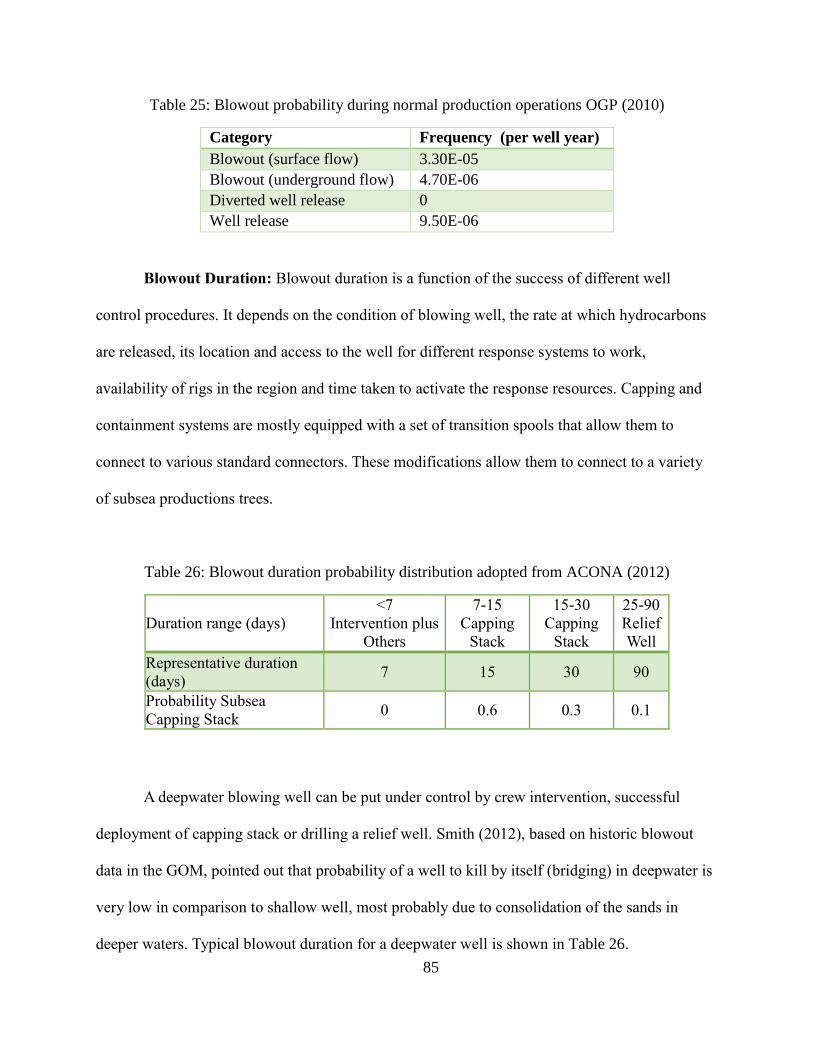
85
Table 25: Blowout probability during normal production operations OGP (2010)
Category Frequency (per well year)
Blowout (surface flow) 3.30E-05
Blowout (underground flow) 4.70E-06
Diverted well release 0
Well release 9.50E-06
Blowout Duration: Blowout duration is a function of the success of different well
control procedures. It depends on the condition of blowing well, the rate at which hydrocarbons
are released, its location and access to the well for different response systems to work,
availability of rigs in the region and time taken to activate the response resources. Capping and
containment systems are mostly equipped with a set of transition spools that allow them to
connect to various standard connectors. These modifications allow them to connect to a variety
of subsea productions trees.
Table 26: Blowout duration probability distribution adopted from ACONA (2012)
Duration range (days)
<7
Intervention plus
Others
7-15
Capping
Stack
15-30
Capping
Stack
25-90
Relief
Well
Representative duration
(days) 7 15 30 90
Probability Subsea
Capping Stack 0 0.6 0.3 0.1
A deepwater blowing well can be put under control by crew intervention, successful
deployment of capping stack or drilling a relief well. Smith (2012), based on historic blowout
data in the GOM, pointed out that probability of a well to kill by itself (bridging) in deepwater is
very low in comparison to shallow well, most probably due to consolidation of the sands in
deeper waters. Typical blowout duration for a deepwater well is shown in Table 26.
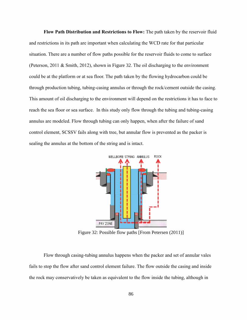
86
Flow Path Distribution and Restrictions to Flow: The path taken by the reservoir fluid
and restrictions in its path are important when calculating the WCD rate for that particular
situation. There are a number of flow paths possible for the reservoir fluids to come to surface
(Peterson, 2011 & Smith, 2012), shown in Figure 32. The oil discharging to the environment
could be at the platform or at sea floor. The path taken by the flowing hydrocarbon could be
through production tubing, tubing-casing annulus or through the rock/cement outside the casing.
This amount of oil discharging to the environment will depend on the restrictions it has to face to
reach the sea floor or sea surface. In this study only flow through the tubing and tubing-casing
annulus are modeled. Flow through tubing can only happen, when after the failure of sand
control element, SCSSV fails along with tree, but annular flow is prevented as the packer is
sealing the annulus at the bottom of the string and is intact.
Figure 32: Possible flow paths [From Petersen (2011)]
Flow through casing-tubing annulus happens when the packer and set of annular vales
fails to stop the flow after sand control element failure. The flow outside the casing and inside
the rock may conservatively be taken as equivalent to the flow inside the tubing, although in
87
reality it may be a fraction of that amount. The case of flow through rock is addressed in chapter-
4 related to underground blowouts.
5.6 Analysis Setup
A commercially available steady state multiphase fluid flow simulator PipeSim, with
black oil composition model was used to estimate the worst case discharge rates with different
set of parametric variations. For heat transfer estimation a linear geothermal gradient was
assumed with surrounding temperature around 40Fo at mud line and it leanly increase to 210F
o
when reservoir depth is reached (a crude assumption, because temperature first decreases and
then increases as we go below the mud line). The specific gravities of oil, gas and water were
taken to be 0.86, 0.67 and 1 respectively. The viscosity was modeled using Vasquez & Beggs
correlation. The roughness of wellbore and casing and drill pipe was assumed to be equivalent of
a steel pipe with value of 0.001 inches. Based on different casing and annular settings, the overall
heat transfer coefficient was taken as 2 Btu/hr/ft2. The pressure at the fluid outlet at seabed is
fixed to be 1395 psi based on the average sea water gradient of 0.465 psi/ft (for saline water,
usually used for GOM) for a water depth of 3000 ft.
5.7 Results and Discussion
5.7.1 Fault Tree Analysis
The results for the Fault Tree Analysis for a deepwater production well are shown in
Figure 33. The high failure rate of primary barrier is mainly due to SCSSV’s control system’s
failure. The delayed response to a potential hazardous event is another area of concern and is one
of the main contributors to primary barrier failure frequency. A careful observation of the
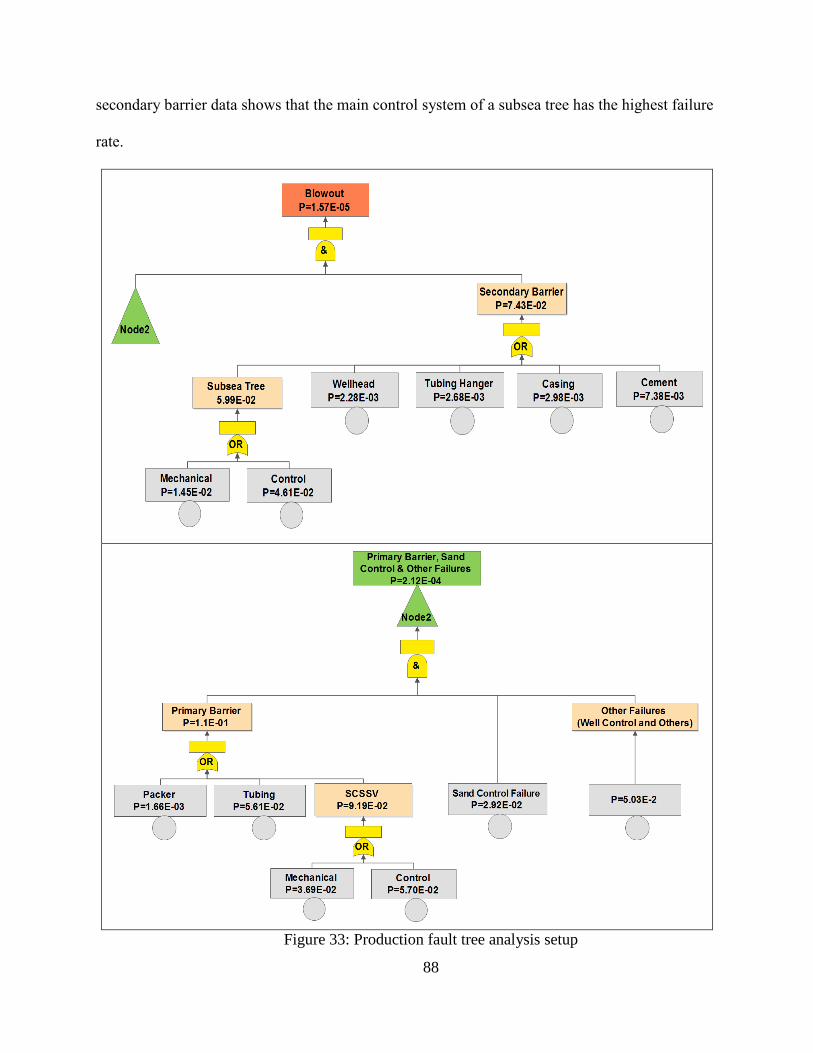
88
secondary barrier data shows that the main control system of a subsea tree has the highest failure
rate.
Figure 33: Production fault tree analysis setup
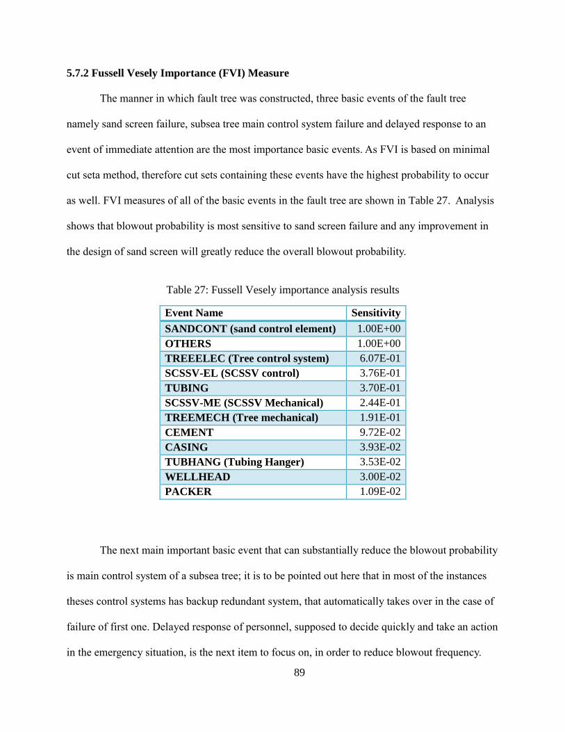
89
5.7.2 Fussell Vesely Importance (FVI) Measure
The manner in which fault tree was constructed, three basic events of the fault tree
namely sand screen failure, subsea tree main control system failure and delayed response to an
event of immediate attention are the most importance basic events. As FVI is based on minimal
cut seta method, therefore cut sets containing these events have the highest probability to occur
as well. FVI measures of all of the basic events in the fault tree are shown in Table 27. Analysis
shows that blowout probability is most sensitive to sand screen failure and any improvement in
the design of sand screen will greatly reduce the overall blowout probability.
Table 27: Fussell Vesely importance analysis results
Event Name Sensitivity
SANDCONT (sand control element) 1.00E+00
OTHERS 1.00E+00
TREEELEC (Tree control system) 6.07E-01
SCSSV-EL (SCSSV control) 3.76E-01
TUBING 3.70E-01
SCSSV-ME (SCSSV Mechanical) 2.44E-01
TREEMECH (Tree mechanical) 1.91E-01
CEMENT 9.72E-02
CASING 3.93E-02
TUBHANG (Tubing Hanger) 3.53E-02
WELLHEAD 3.00E-02
PACKER 1.09E-02
The next main important basic event that can substantially reduce the blowout probability
is main control system of a subsea tree; it is to be pointed out here that in most of the instances
theses control systems has backup redundant system, that automatically takes over in the case of
failure of first one. Delayed response of personnel, supposed to decide quickly and take an action
in the emergency situation, is the next item to focus on, in order to reduce blowout frequency.
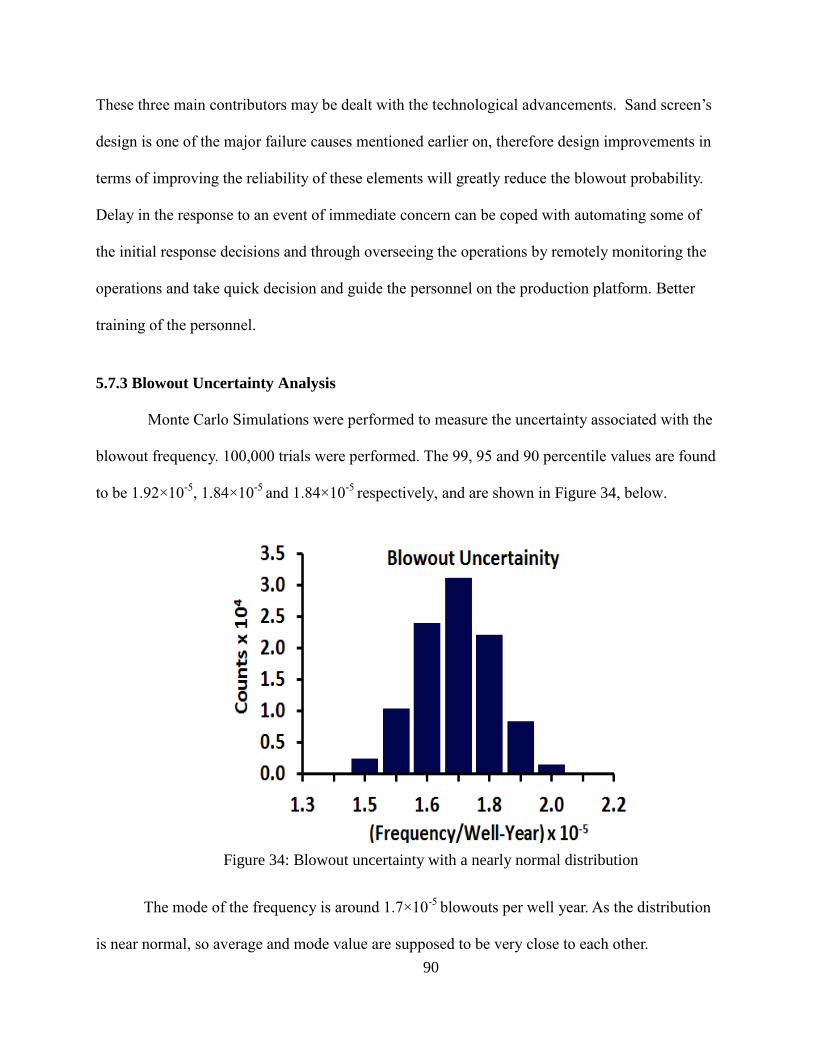
90
These three main contributors may be dealt with the technological advancements. Sand screen’s
design is one of the major failure causes mentioned earlier on, therefore design improvements in
terms of improving the reliability of these elements will greatly reduce the blowout probability.
Delay in the response to an event of immediate concern can be coped with automating some of
the initial response decisions and through overseeing the operations by remotely monitoring the
operations and take quick decision and guide the personnel on the production platform. Better
training of the personnel.
5.7.3 Blowout Uncertainty Analysis
Monte Carlo Simulations were performed to measure the uncertainty associated with the
blowout frequency. 100,000 trials were performed. The 99, 95 and 90 percentile values are found
to be 1.92×10⁻⁵
, 1.84×10⁻⁵
and 1.84×10⁻⁵
respectively, and are shown in Figure 34, below.
Figure 34: Blowout uncertainty with a nearly normal distribution
The mode of the frequency is around 1.7×10⁻⁵
blowouts per well year. As the distribution
is near normal, so average and mode value are supposed to be very close to each other.
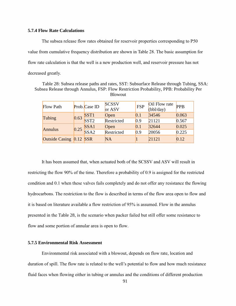
91
5.7.4 Flow Rate Calculations
The subsea release flow rates obtained for reservoir properties corresponding to P50
value from cumulative frequency distribution are shown in Table 28. The basic assumption for
flow rate calculation is that the well is a new production well, and reservoir pressure has not
decreased greatly.
Table 28: Subsea release paths and rates, SST: Subsurface Release through Tubing, SSA:
Subsea Release through Annulus, FSP: Flow Restriction Probability, PPB: Probability Per
Blowout
Flow Path Prob. Case ID SCSSV
or ASV FSP
Oil Flow rate
(bbl/day) PPB
Tubing 0.63 SST1 Open 0.1 34546 0.063
SST2 Restricted 0.9 21121 0.567
Annulus 0.25 SSA1 Open 0.1 32644 0.025
SSA2 Restricted 0.9 20056 0.225
Outside Casing 0.12 SSR NA 1 21121 0.12
It has been assumed that, when actuated both of the SCSSV and ASV will result in
restricting the flow 90% of the time. Therefore a probability of 0.9 is assigned for the restricted
condition and 0.1 when these valves fails completely and do not offer any resistance the flowing
hydrocarbons. The restriction to the flow is described in terms of the flow area open to flow and
it is based on literature available a flow restriction of 95% is assumed. Flow in the annulus
presented in the Table 28, is the scenario when packer failed but still offer some resistance to
flow and some portion of annular area is open to flow.
5.7.5 Environmental Risk Assessment
Environmental risk associated with a blowout, depends on flow rate, location and
duration of spill. The flow rate is related to the well’s potential to flow and how much resistance
fluid faces when flowing either in tubing or annulus and the conditions of different production
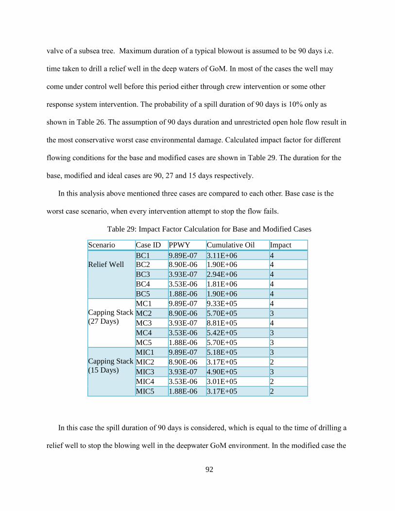
92
valve of a subsea tree. Maximum duration of a typical blowout is assumed to be 90 days i.e.
time taken to drill a relief well in the deep waters of GoM. In most of the cases the well may
come under control well before this period either through crew intervention or some other
response system intervention. The probability of a spill duration of 90 days is 10% only as
shown in Table 26. The assumption of 90 days duration and unrestricted open hole flow result in
the most conservative worst case environmental damage. Calculated impact factor for different
flowing conditions for the base and modified cases are shown in Table 29. The duration for the
base, modified and ideal cases are 90, 27 and 15 days respectively.
In this analysis above mentioned three cases are compared to each other. Base case is the
worst case scenario, when every intervention attempt to stop the flow fails.
Table 29: Impact Factor Calculation for Base and Modified Cases
Scenario Case ID PPWY Cumulative Oil
Volume (bbls)
Impact
Factor
Relief Well
BC1 9.89E-07 3.11E+06 4
BC2 8.90E-06 1.90E+06 4
BC3 3.93E-07 2.94E+06 4
BC4 3.53E-06 1.81E+06 4
BC5 1.88E-06 1.90E+06 4
Capping Stack
(27 Days)
MC1 9.89E-07 9.33E+05 4
MC2 8.90E-06 5.70E+05 3
MC3 3.93E-07 8.81E+05 4
MC4 3.53E-06 5.42E+05 3
MC5 1.88E-06 5.70E+05 3
Capping Stack
(15 Days)
MIC1 9.89E-07 5.18E+05 3
MIC2 8.90E-06 3.17E+05 2
MIC3 3.93E-07 4.90E+05 3
MIC4 3.53E-06 3.01E+05 2
MIC5 1.88E-06 3.17E+05 2
In this case the spill duration of 90 days is considered, which is equal to the time of drilling a
relief well to stop the blowing well in the deepwater GoM environment. In the modified case the
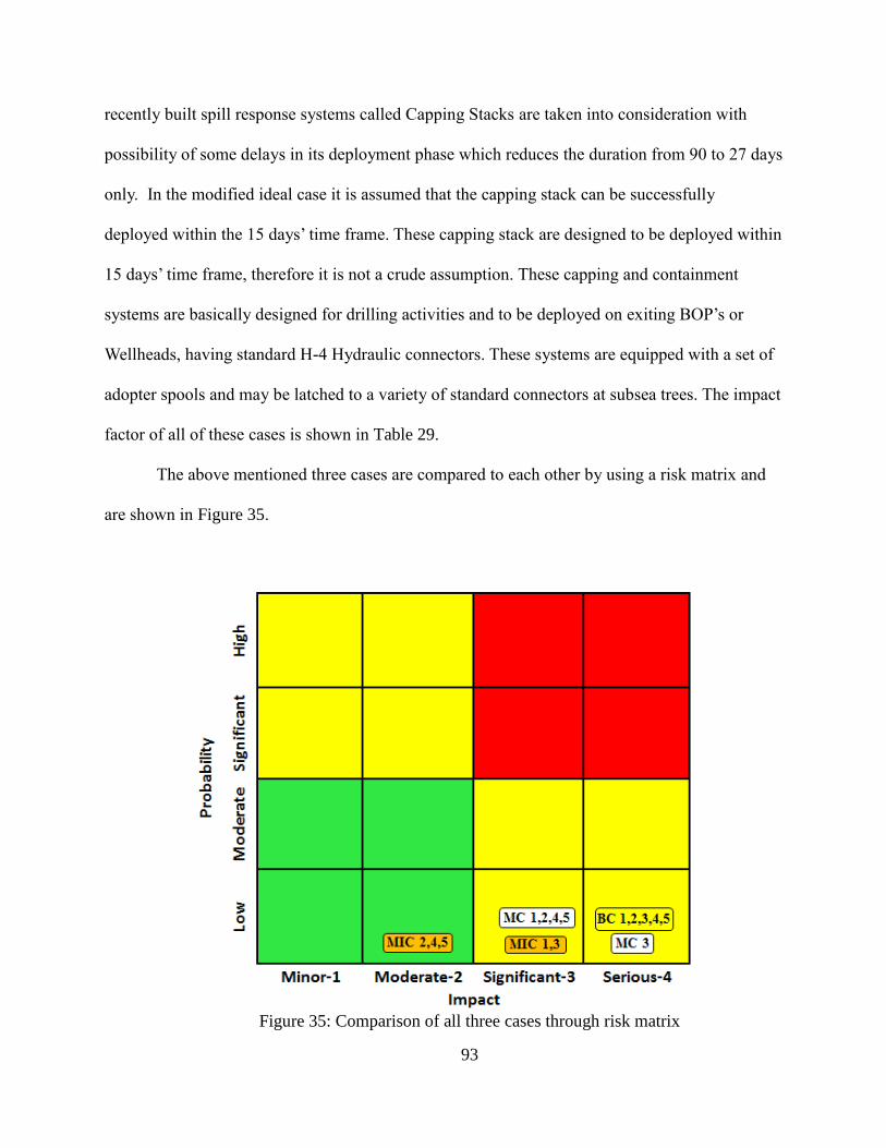
93
recently built spill response systems called Capping Stacks are taken into consideration with
possibility of some delays in its deployment phase which reduces the duration from 90 to 27 days
only. In the modified ideal case it is assumed that the capping stack can be successfully
deployed within the 15 days’ time frame. These capping stack are designed to be deployed within
15 days’ time frame, therefore it is not a crude assumption. These capping and containment
systems are basically designed for drilling activities and to be deployed on exiting BOP’s or
Wellheads, having standard H-4 Hydraulic connectors. These systems are equipped with a set of
adopter spools and may be latched to a variety of standard connectors at subsea trees. The impact
factor of all of these cases is shown in Table 29.
The above mentioned three cases are compared to each other by using a risk matrix and
are shown in Figure 35.
Figure 35: Comparison of all three cases through risk matrix
94
The entire base subcases results in the category of serious impact, but due to their very
low frequency of occurrences, when an overall risk is computed through the product of
probability and consequences, their risk level fall in the yellow region, in which operations are
conducted with extra safety precautions. The use of the capping stack significantly altered the
impact of large spill, by reducing the spill duration and as a result less volume is released to the
environment. The modified ideal case is the case when capping stack is successfully deployed
within the 15 days intended response time, and as a result it shifts the impact from significant to
moderate. This analysis shows the significant contributions that technological improvements can
bring in order to reduce large oil spills in the GoM.
There have been technological improvements in other area of production systems as well,
that may result in further reducing the frequency of primary and secondary barrier failure rates.
5.8 Concluding Remarks for Scenario-3
The QRA study of a deepwater production well has been performed and key contributors
to overall system safety have been identified through fault tree analysis.
Sensitivity analysis of all of the basic events in the constructed Fault Tree for a sand
screen failure leading to blowout was conducted. It turned out to that the three most
important basic events contributing to the frequency of blowout are sand screen failures,
subsea production tree’s control system failure and well control/other failures.
It has been suggested by other researchers that the design improvements of the sand screen
will greatly reduce their failure rates and in turn blowout frequency associated with
production well, as it is one of the most sensitive/important basic event in the system
setup, considered for this scenario.
95
Subsea production tree’s control system is the second most important basic event in the
system, and even a small improvement in the reliability of control system will greatly
influence the blowout frequency of the entire system.
Monte Carlo simulation results for blowout probability show a range of values between
1.54-2.0 ×10⁻⁵
per well-year, when each of the basic events is varied by ±10%.
A WCD rate of 34,546 BOPD was estimated using multiphase fluid simulations and it is
well within the fluid handling capacity of newly built response systems called capping and
containment systems. Newly built response systems are effective in reducing the risk of
large oil spill in deepwater environments. Additional tools like adopter spools may be
needed to connect capping stack to subsea trees with different connector profiles.
The blowout frequency modeled by FTA is based on the historical data and therefore it is a
conservative estimate. When recent technological improvements are incorporated into
FTA, the blowout frequency will be reduced, as in the past few years there have been
major improvements in well safety related procedures. New regulatory requirements,
equipment reliability improvements and extensive training of crew, all of these will
contribute in lowering the blowout frequency estimates.
96
CHAPTER 6: A REVIEW OF OIL SPILL RISK ASSOCIATED WITH FPSO
DEPLOYMENT IN GOM (SCENARIO-4)
FPSO stands for Floating Production Storage and Offloading vessels. They are essentially
ship-shaped vessels; either specially built or converted tankers. They produce, store and transport
hydrocarbons to either shuttle tankers or deepwater pipeline terminals. The main advantages of
FPSO as compared to other offshore platforms are
They allow production far deeper than fixed platforms. Most of the FPSO’s have been
deployed to deepwater fields, as they are nearly water depth insensitive as compared to other
offshore production platforms.
They allow development of short-lived, marginal fields in remote locations where fixed
platform are not feasible economically.
They can process large amount of hydrocarbons and have huge storage capacity as well, and
the processed fluids are usually transported by shuttle tankers.
They eliminate the need of cost associated with long pipelines to onshore terminals,
especially in ultra-deepwater where seabed pipelines are not cost effective.
They are particularly effective in remote deepwater.
They can be relocated to new locations and reused easily.
In terms of spill potential the following capabilities of the FPSO are different than other
offshore platforms
1. Station Keeping and buoyancy
2. Shuttle tanker Transport
3. Large storage capacity
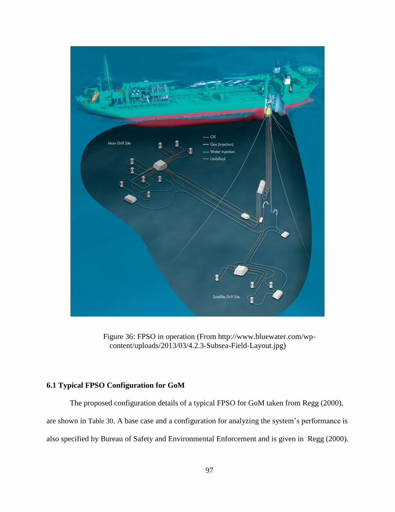
97
Figure 36: FPSO in operation (From http://www.bluewater.com/wp-
content/uploads/2013/03/4.2.3-Subsea-Field-Layout.jpg)
6.1 Typical FPSO Configuration for GoM
The proposed configuration details of a typical FPSO for GoM taken from Regg (2000),
are shown in Table 30. A base case and a configuration for analyzing the system’s performance is
also specified by Bureau of Safety and Environmental Enforcement and is given in Regg (2000).
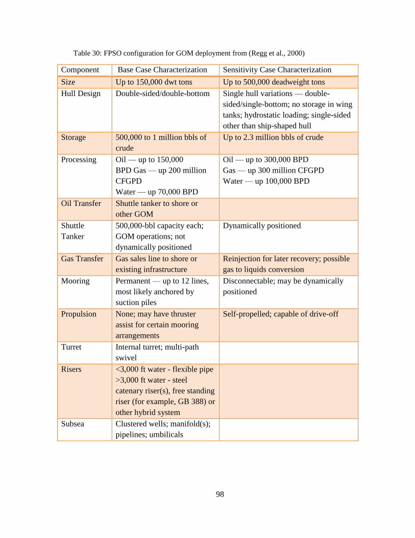
98
Table 30: FPSO configuration for GOM deployment from (Regg et al., 2000)
Component Base Case Characterization Sensitivity Case Characterization
Size Up to 150,000 dwt tons Up to 500,000 deadweight tons
Hull Design Double-sided/double-bottom Single hull variations — double-
sided/single-bottom; no storage in wing
tanks; hydrostatic loading; single-sided
other than ship-shaped hull
Storage 500,000 to 1 million bbls of
crude
Up to 2.3 million bbls of crude
Processing Oil — up to 150,000
BPD Gas — up 200 million
CFGPD
Water — up 70,000 BPD
Oil — up to 300,000 BPD
Gas — up 300 million CFGPD
Water — up 100,000 BPD
Oil Transfer Shuttle tanker to shore or
other GOM
Shuttle
Tanker
500,000-bbl capacity each;
GOM operations; not
dynamically positioned
Dynamically positioned
Gas Transfer Gas sales line to shore or
existing infrastructure
Reinjection for later recovery; possible
gas to liquids conversion
Mooring Permanent — up to 12 lines,
most likely anchored by
suction piles
Disconnectable; may be dynamically
positioned
Propulsion None; may have thruster
assist for certain mooring
arrangements
Self-propelled; capable of drive-off
Turret Internal turret; multi-path
swivel
Risers <3,000 ft water - flexible pipe
>3,000 ft water - steel
catenary riser(s), free standing
riser (for example, GB 388) or
other hybrid system
Subsea Clustered wells; manifold(s);
pipelines; umbilicals
99
The data used in this scenario is adopted from sensitivity case characterization
configuration given in Table 30. The risk associated with the deployment of FPSO are
comparable to other production facilities with some added concerns about the station keeping,
large storage capacity and collision with shuttle tanker. Gilbert et al. (2001), conducted the
comparative analysis of FPSO with other deepwater developments and concluded that the oil
spill and other associated risk with FPSO are comparable to other facilities and major
contribution of spill may be due to transportation of oil using shuttle tankers. Spill sources would
be the same as for other production facilities: process train (separators, piping, small volume
storage tanks), pipelines, and riser/wellbore. The large volume storage associated with an FPSO,
transfer operations (from FPSO or other loading facility to the shuttle tanker), and shuttle tanker
transport are areas that differ from typical GOM developments (platforms, subsea, other FPS’s).
A quantitative risk assessment study conducted by Overfield et al., (2000) for FPSO safety,
points out that the main risk to the personnel is dominated by fires, explosions and cargo tank
explosion. While assets risk are posed by the collision of shuttle tanker, riser leaks, subsea
pipeline damage and turret operations. The focus of the study is the impact analysis of the
following factors specific to FPSO.
Station Keeping FPSO
Transportation Spill Analysis
Large Storage Capacity of FPSO
These are discussed in detail in the following sections.
6.2 Station Keeping
Position/station keeping is one of the main differences between FPSO and offshore
production platform types, due to FPSO’s dynamic positioning system. Two options exist for
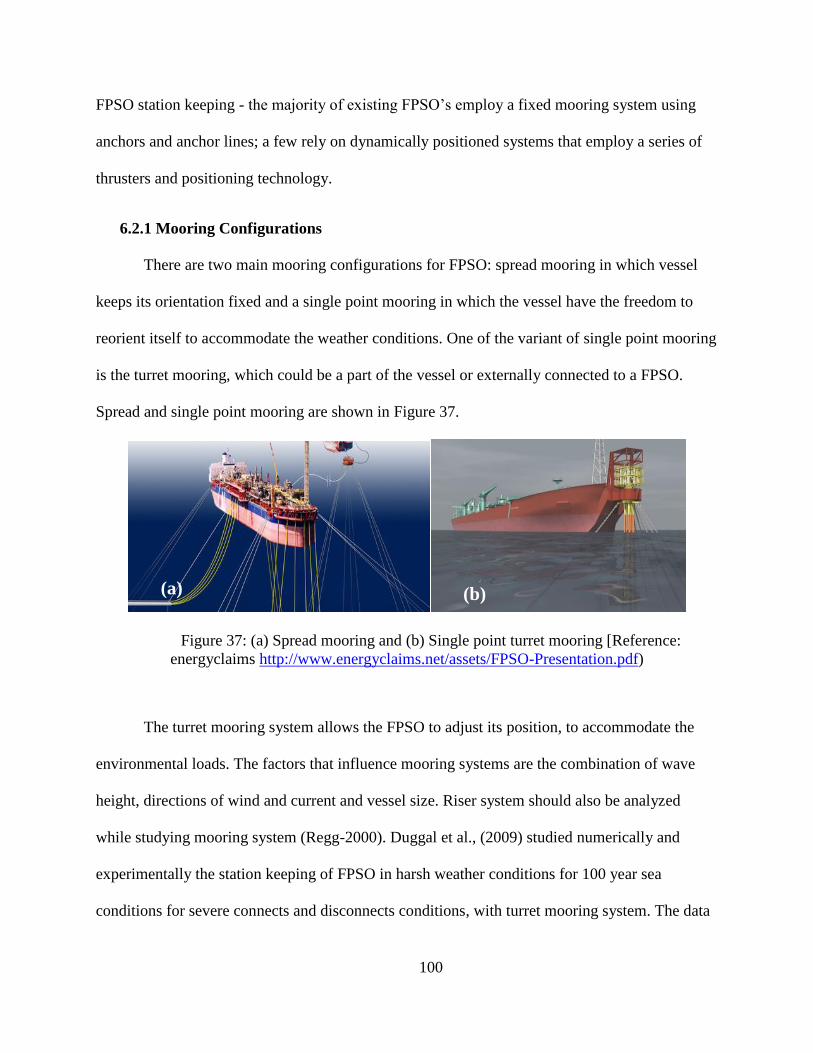
100
FPSO station keeping - the majority of existing FPSO’s employ a fixed mooring system using
anchors and anchor lines; a few rely on dynamically positioned systems that employ a series of
thrusters and positioning technology.
6.2.1 Mooring Configurations
There are two main mooring configurations for FPSO: spread mooring in which vessel
keeps its orientation fixed and a single point mooring in which the vessel have the freedom to
reorient itself to accommodate the weather conditions. One of the variant of single point mooring
is the turret mooring, which could be a part of the vessel or externally connected to a FPSO.
Spread and single point mooring are shown in Figure 37.
Figure 37: (a) Spread mooring and (b) Single point turret mooring [Reference:
energyclaims http://www.energyclaims.net/assets/FPSO-Presentation.pdf)
The turret mooring system allows the FPSO to adjust its position, to accommodate the
environmental loads. The factors that influence mooring systems are the combination of wave
height, directions of wind and current and vessel size. Riser system should also be analyzed
while studying mooring system (Regg-2000). Duggal et al., (2009) studied numerically and
experimentally the station keeping of FPSO in harsh weather conditions for 100 year sea
conditions for severe connects and disconnects conditions, with turret mooring system. The data
(a) (b)
101
for the actual FPSO in severe weather conditions showed that these systems performed reliably
in severe weather conditions to disconnect and connect back to subsea installations.
6.2.2 FPSO Roll motion effect on Mooring
It has been reported that hulls of FPSO have been exposed to excessive roll motion up to
20 degrees amplitude (Kinnas, 2005). This excessive motion may result in damaging the
mooring lines and halting the operations as well. The solution to this problem has been suggested
by Kinnas (2005) as to install of bilge keels on these hulls.
6.2.3 FPSO Yawing Motion
In a study conducted by Kim (2004), a coupled vessel-riser-mooring dynamic system
was analyzed experimentally. A scaled down model on a 1:60 Scale was used. It was concluded
that when mooring dynamic effects are significant, the dynamic mooring tension can be under
predicted with truncated mooring system. Rocha et al., in 2010 performed and FEMCA analysis
of different systems contributing in maintaining the balance of FPSO in the case of an
emergency situation. They pointed out that amongst the systems they selected for the study,
Safety Interlock and Automation System (SAIS) was the least reliable systems and they
recommended the design re-evaluation if possible for SAIS. Holdbrook in 2004 conducted a risk
based assessment of hull structure and pointed out that the cracking probability of hull structure
for FPSO may be higher as compared to fixed offshore structures, as there are more stresses
concentrating feature in a typical FPSO hull. A major factor for these cracks may be stresses
caused by improper loading and unloading sequence (OGP-Report # 377).
6.3 Fuel Offloading Operations
Most of the FPSOs offload the hydrocarbons to shuttle tankers directly. The direct
transport is usually achieved through tandem offloading or side by side offloading. The tandem
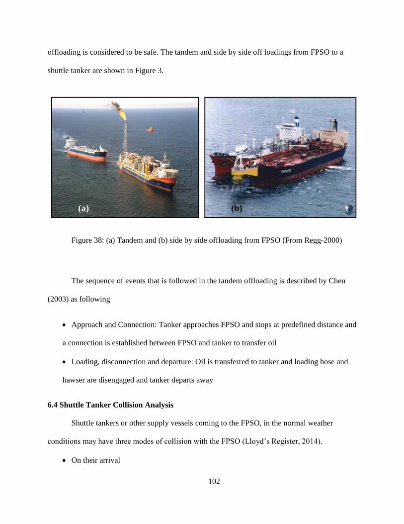
102
offloading is considered to be safe. The tandem and side by side off loadings from FPSO to a
shuttle tanker are shown in Figure 3.
Figure 38: (a) Tandem and (b) side by side offloading from FPSO (From Regg-2000)
The sequence of events that is followed in the tandem offloading is described by Chen
(2003) as following
Approach and Connection: Tanker approaches FPSO and stops at predefined distance and
a connection is established between FPSO and tanker to transfer oil
Loading, disconnection and departure: Oil is transferred to tanker and loading hose and
hawser are disengaged and tanker departs away
6.4 Shuttle Tanker Collision Analysis
Shuttle tankers or other supply vessels coming to the FPSO, in the normal weather
conditions may have three modes of collision with the FPSO (Lloyd’s Register, 2014).
On their arrival
(a) (b)
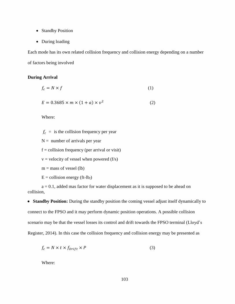
103
Standby Position
During loading
Each mode has its own related collision frequency and collision energy depending on a number
of factors being involved
During Arrival
𝑓𝑐 = 𝑁 × 𝑓 (1)
𝐸 = 0.3685 × 𝑚 × (1 + 𝑎) × 𝑣2 (2)
Where:
𝑓𝑐 = is the collision frequency per year
N = number of arrivals per year
f = collision frequency (per arrival or visit)
v = velocity of vessel when powered (f/s)
m = mass of vessel (lb)
E = collision energy (ft-lbf)
a = 0.1, added mas factor for water displacement as it is supposed to be ahead on
collision,
Standby Position: During the standby position the coming vessel adjust itself dynamically to
connect to the FPSO and it may perform dynamic position operations. A possible collision
scenario may be that the vessel losses its control and drift towards the FPSO terminal (Lloyd’s
Register, 2014). In this case the collision frequency and collision energy may be presented as
𝑓𝑐 = 𝑁 × 𝑡 × 𝑓𝐷𝑟𝑖𝑓𝑡 × 𝑃 (3)
Where:
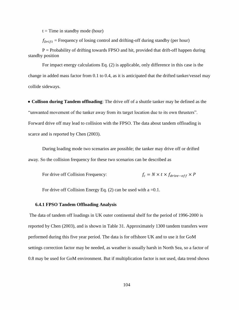
104
t = Time in standby mode (hour)
𝑓𝐷𝑟𝑖𝑓𝑡 = Frequency of losing control and drifting-off during standby (per hour)
P = Probability of drifting towards FPSO and hit, provided that drift-off happen during
standby position
For impact energy calculations Eq. (2) is applicable, only difference in this case is the
change in added mass factor from 0.1 to 0.4, as it is anticipated that the drifted tanker/vessel may
collide sideways.
Collison during Tandem offloading: The drive off of a shuttle tanker may be defined as the
“unwanted movement of the tanker away from its target location due to its own thrusters”.
Forward drive off may lead to collision with the FPSO. The data about tandem offloading is
scarce and is reported by Chen (2003).
During loading mode two scenarios are possible; the tanker may drive off or drifted
away. So the collision frequency for these two scenarios can be described as
For drive off Collision Frequency: 𝑓𝑐 = 𝑁 × 𝑡 × 𝑓𝑑𝑟𝑖𝑣𝑒−𝑜𝑓𝑓 × 𝑃
For drive off Collision Energy Eq. (2) can be used with a =0.1.
6.4.1 FPSO Tandem Offloading Analysis
The data of tandem off loadings in UK outer continental shelf for the period of 1996-2000 is
reported by Chen (2003), and is shown in Table 31. Approximately 1300 tandem transfers were
performed during this five year period. The data is for offshore UK and to use it for GoM
settings correction factor may be needed, as weather is usually harsh in North Sea, so a factor of
0.8 may be used for GoM environment. But if multiplication factor is not used, data trend shows
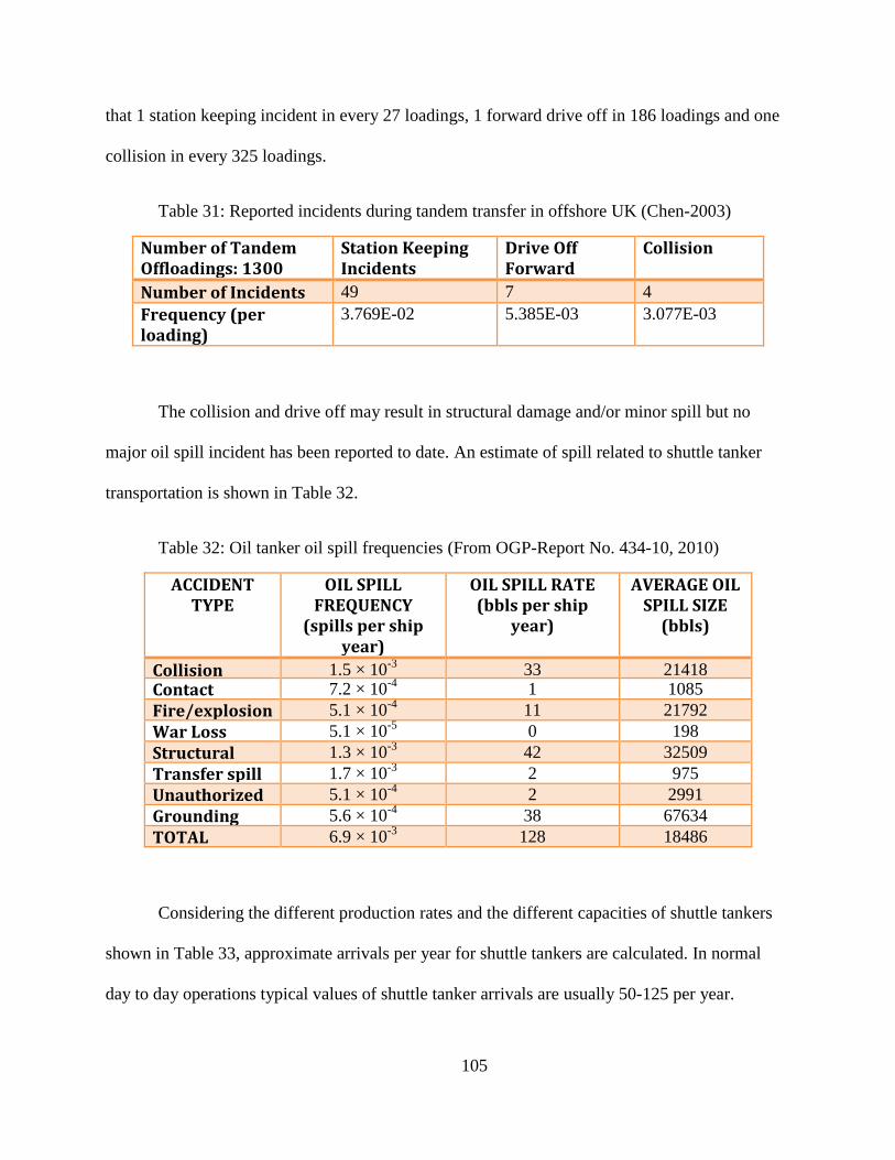
105
that 1 station keeping incident in every 27 loadings, 1 forward drive off in 186 loadings and one
collision in every 325 loadings.
Table 31: Reported incidents during tandem transfer in offshore UK (Chen-2003)
Number of Tandem Offloadings: 1300
Station Keeping Incidents
Drive Off Forward
Collision
Number of Incidents 49 7 4
Frequency (per loading)
3.769E-02 5.385E-03 3.077E-03
The collision and drive off may result in structural damage and/or minor spill but no
major oil spill incident has been reported to date. An estimate of spill related to shuttle tanker
transportation is shown in Table 32.
Table 32: Oil tanker oil spill frequencies (From OGP-Report No. 434-10, 2010)
ACCIDENT TYPE
OIL SPILL FREQUENCY
(spills per ship year)
OIL SPILL RATE (bbls per ship
year)
AVERAGE OIL SPILL SIZE
(bbls)
Collision 1.5 × 10⁻³
33 21418
Contact 7.2 × 10⁻⁴
1 1085
Fire/explosion 5.1 × 10⁻⁴
11 21792
War Loss 5.1 × 10⁻⁵
0 198
Structural failure
1.3 × 10⁻³
42 32509
Transfer spill 1.7 × 10⁻³
2 975
Unauthorized discharge
5.1 × 10⁻⁴
2 2991
Grounding 5.6 × 10⁻⁴
38 67634
TOTAL 6.9 × 10⁻³
128 18486
Considering the different production rates and the different capacities of shuttle tankers
shown in Table 33, approximate arrivals per year for shuttle tankers are calculated. In normal
day to day operations typical values of shuttle tanker arrivals are usually 50-125 per year.
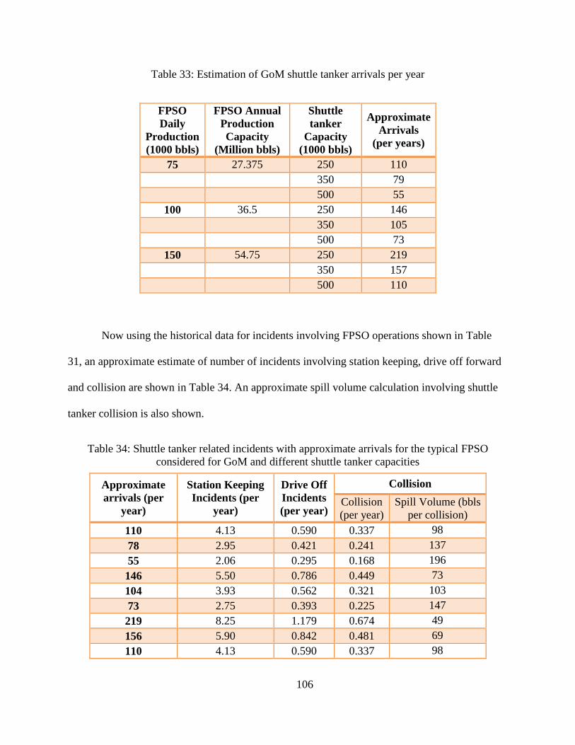
106
Table 33: Estimation of GoM shuttle tanker arrivals per year
FPSO
Daily
Production
(1000 bbls)
FPSO Annual
Production
Capacity
(Million bbls)
Shuttle
tanker
Capacity
(1000 bbls)
Approximate
Arrivals
(per years)
75 27.375 250 110
350 79
500 55
100 36.5 250 146
350 105
500 73
150 54.75 250 219
350 157
500 110
Now using the historical data for incidents involving FPSO operations shown in Table
31, an approximate estimate of number of incidents involving station keeping, drive off forward
and collision are shown in Table 34. An approximate spill volume calculation involving shuttle
tanker collision is also shown.
Table 34: Shuttle tanker related incidents with approximate arrivals for the typical FPSO
considered for GoM and different shuttle tanker capacities
Approximate
arrivals (per
year)
Station Keeping
Incidents (per
year)
Drive Off
Incidents
(per year)
Collision
Collision
(per year)
Spill Volume (bbls
per collision)
110 4.13 0.590 0.337 98
78 2.95 0.421 0.241 137
55 2.06 0.295 0.168 196
146 5.50 0.786 0.449 73
104 3.93 0.562 0.321 103
73 2.75 0.393 0.225 147
219 8.25 1.179 0.674 49
156 5.90 0.842 0.481 69
110 4.13 0.590 0.337 98
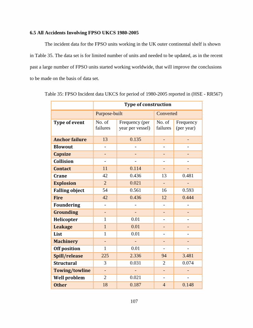
107
6.5 All Accidents Involving FPSO UKCS 1980-2005
The incident data for the FPSO units working in the UK outer continental shelf is shown
in Table 35. The data set is for limited number of units and needed to be updated, as in the recent
past a large number of FPSO units started working worldwide, that will improve the conclusions
to be made on the basis of data set.
Table 35: FPSO Incident data UKCS for period of 1980-2005 reported in (HSE - RR567)
Type of construction
Purpose-built Converted
Type of event No. of
failures
Frequency (per
year per vessel)
No. of
failures
Frequency
(per year)
Anchor failure 13 0.135 - -
Blowout - - - -
Capsize - - - -
Collision - - - -
Contact 11 0.114 - -
Crane 42 0.436 13 0.481
Explosion 2 0.021 - -
Falling object 54 0.561 16 0.593
Fire 42 0.436 12 0.444
Foundering - - - -
Grounding - - - -
Helicopter 1 0.01 - -
Leakage 1 0.01 - -
List 1 0.01 - -
Machinery - - - -
Off position 1 0.01 - -
Spill/release 225 2.336 94 3.481
Structural 3 0.031 2 0.074
Towing/towline - - - -
Well problem 2 0.021 - -
Other 18 0.187 4 0.148
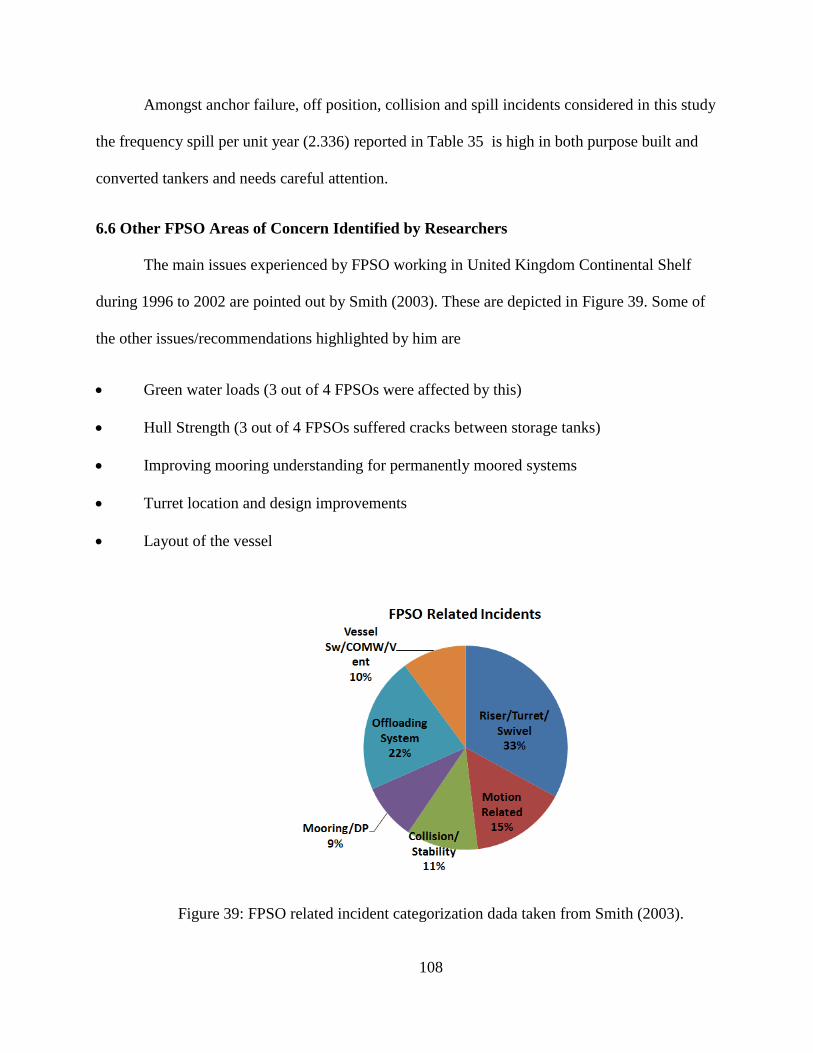
108
Amongst anchor failure, off position, collision and spill incidents considered in this study
the frequency spill per unit year (2.336) reported in Table 35 is high in both purpose built and
converted tankers and needs careful attention.
6.6 Other FPSO Areas of Concern Identified by Researchers
The main issues experienced by FPSO working in United Kingdom Continental Shelf
during 1996 to 2002 are pointed out by Smith (2003). These are depicted in Figure 39. Some of
the other issues/recommendations highlighted by him are
Green water loads (3 out of 4 FPSOs were affected by this)
Hull Strength (3 out of 4 FPSOs suffered cracks between storage tanks)
Improving mooring understanding for permanently moored systems
Turret location and design improvements
Layout of the vessel
Figure 39: FPSO related incident categorization dada taken from Smith (2003).
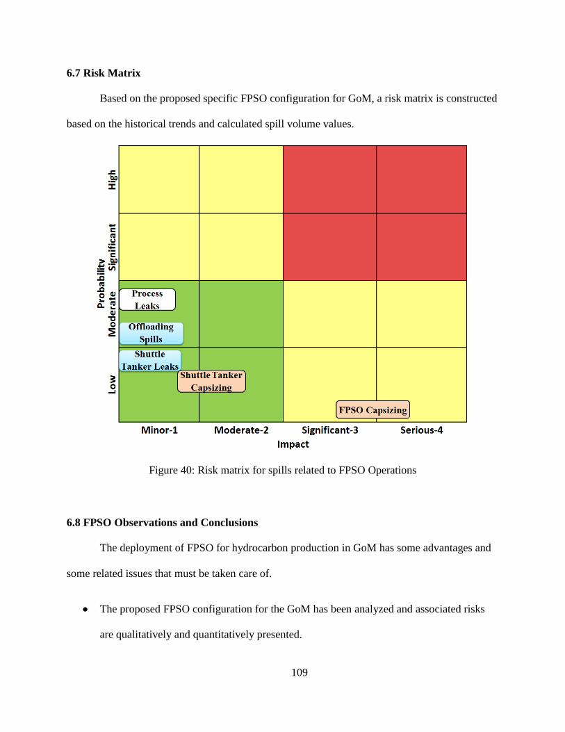
109
6.7 Risk Matrix
Based on the proposed specific FPSO configuration for GoM, a risk matrix is constructed
based on the historical trends and calculated spill volume values.
Figure 40: Risk matrix for spills related to FPSO Operations
6.8 FPSO Observations and Conclusions
The deployment of FPSO for hydrocarbon production in GoM has some advantages and
some related issues that must be taken care of.
The proposed FPSO configuration for the GoM has been analyzed and associated risks
are qualitatively and quantitatively presented.
110
It has been reported by previous researchers that risk associated with FPSO deployment
in the GoM are comparable to other production platforms and FPSO needs additional
considerations due to its large fluid storage capacity, station keeping requirements and oil
transportation mechanism.
Most of the historical oil spills associated with FPSOs operations actually happened
during oil transportation from FPSO to onshore facilities by shuttle tankers.
Reported oil spill incidents involving FPSO vessel are mainly due to loss of its position
keeping and during fuel offloading process. These spills are of very small quantity as
compared to shuttle tanker spills.
An example calculation based on the proposed configuration of FPSO for GoM has been
performed to estimate the frequency of shuttle tanker collision with the FPSO and related
spill amount.
Analysis shows that only small amount 100-200 bbl of oil spills will result due to shuttle
collision with other vessels including FPSO, and maximum spill amount will result when
the shuttle tanker capsizes while carrying hydrocarbons from FPSO to onshore facilities.
The probability of FPSO capsizing is very low, as there are no reported incidents. But if it
is the case, a large oil spill will most probably be expected due to its large fluid storage
capacity and other possible damages that can occur to wellheads or subsea installations.
Amongst the spill response technology, oil skimmers boats seem to be the most
appropriate for spills involving shuttle tankers as these are the most frequent spills
involving production from FPSO.
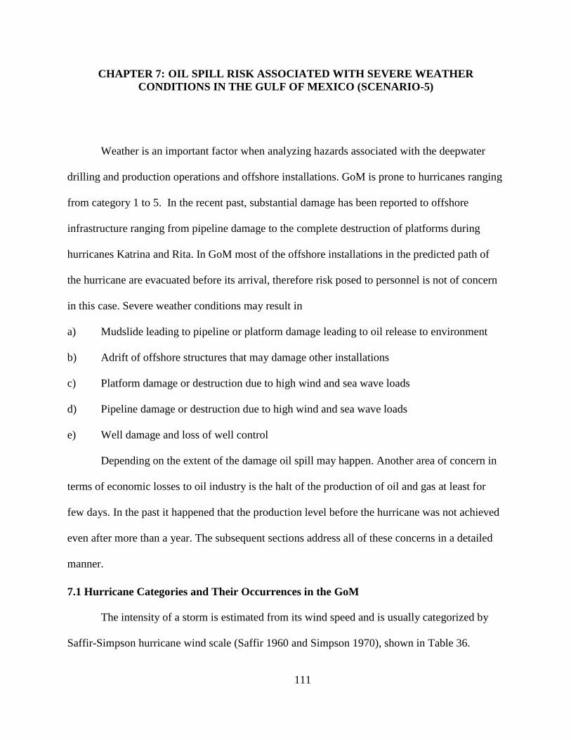
111
CHAPTER 7: OIL SPILL RISK ASSOCIATED WITH SEVERE WEATHER
CONDITIONS IN THE GULF OF MEXICO (SCENARIO-5)
Weather is an important factor when analyzing hazards associated with the deepwater
drilling and production operations and offshore installations. GoM is prone to hurricanes ranging
from category 1 to 5. In the recent past, substantial damage has been reported to offshore
infrastructure ranging from pipeline damage to the complete destruction of platforms during
hurricanes Katrina and Rita. In GoM most of the offshore installations in the predicted path of
the hurricane are evacuated before its arrival, therefore risk posed to personnel is not of concern
in this case. Severe weather conditions may result in
a) Mudslide leading to pipeline or platform damage leading to oil release to environment
b) Adrift of offshore structures that may damage other installations
c) Platform damage or destruction due to high wind and sea wave loads
d) Pipeline damage or destruction due to high wind and sea wave loads
e) Well damage and loss of well control
Depending on the extent of the damage oil spill may happen. Another area of concern in
terms of economic losses to oil industry is the halt of the production of oil and gas at least for
few days. In the past it happened that the production level before the hurricane was not achieved
even after more than a year. The subsequent sections address all of these concerns in a detailed
manner.
7.1 Hurricane Categories and Their Occurrences in the GoM
The intensity of a storm is estimated from its wind speed and is usually categorized by
Saffir-Simpson hurricane wind scale (Saffir 1960 and Simpson 1970), shown in Table 36.
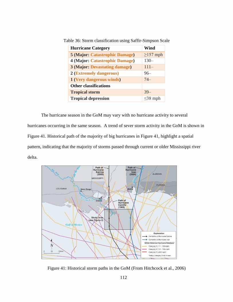
112
Table 36: Storm classification using Saffir-Simpson Scale
Hurricane Category Wind
Speed 5 (Major: Catastrophic Damage) ≥157 mph
4 (Major: Catastrophic Damage) 130–
156 mph 3 (Major: Devastating damage) 111–
129 mph 2 (Extremely dangerous) 96–
110 mph 1 (Very dangerous winds) 74–
95 mph Other classifications
Tropical storm 39–
73 mph Tropical depression ≤38 mph
The hurricane season in the GoM may vary with no hurricane activity to several
hurricanes occurring in the same season. A trend of sever storm activity in the GoM is shown in
Figure 41. Historical path of the majority of big hurricanes in Figure 41, highlight a spatial
pattern, indicating that the majority of storms passed through current or older Mississippi river
delta.
Figure 41: Historical storm paths in the GoM (From Hitchcock et al., 2006)
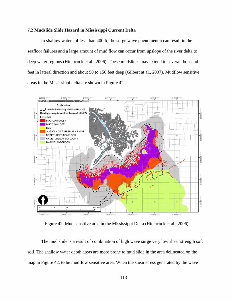
113
7.2 Mudslide Slide Hazard in Mississippi Current Delta
In shallow waters of less than 400 ft, the surge wave phenomenon can result in the
seafloor failures and a large amount of mud flow can occur from upslope of the river delta to
deep water regions (Hitchcock et al., 2006). These mudslides may extend to several thousand
feet in lateral direction and about 50 to 150 feet deep (Gilbert at al., 2007). Mudflow sensitive
areas in the Mississippi delta are shown in Figure 42.
Figure 42: Mud sensitive area in the Mississippi Delta (Hitchcock et al., 2006)
The mud slide is a result of combination of high wave surge very low shear strength soft
soil. The shallow water depth areas are more prone to mud slide in the area delineated on the
map in Figure 42, to be mudflow sensitive area. When the shear stress generated by the wave
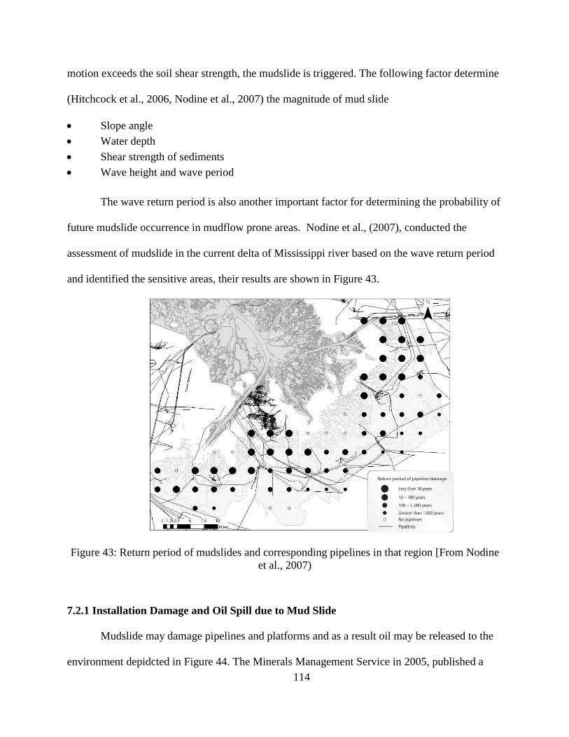
114
motion exceeds the soil shear strength, the mudslide is triggered. The following factor determine
(Hitchcock et al., 2006, Nodine et al., 2007) the magnitude of mud slide
Slope angle
Water depth
Shear strength of sediments
Wave height and wave period
The wave return period is also another important factor for determining the probability of
future mudslide occurrence in mudflow prone areas. Nodine et al., (2007), conducted the
assessment of mudslide in the current delta of Mississippi river based on the wave return period
and identified the sensitive areas, their results are shown in Figure 43.
Figure 43: Return period of mudslides and corresponding pipelines in that region [From Nodine
et al., 2007)
7.2.1 Installation Damage and Oil Spill due to Mud Slide
Mudslide may damage pipelines and platforms and as a result oil may be released to the
environment depidcted in Figure 44. The Minerals Management Service in 2005, published a
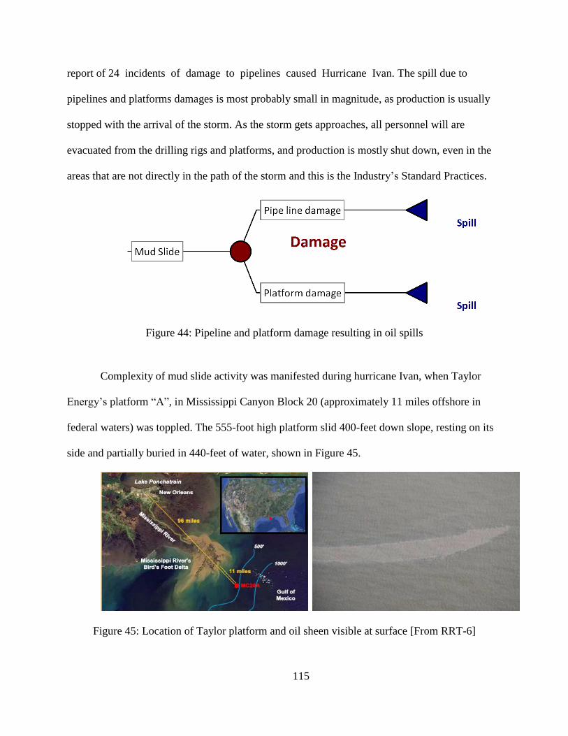
115
report of 24 incidents of damage to pipelines caused Hurricane Ivan. The spill due to
pipelines and platforms damages is most probably small in magnitude, as production is usually
stopped with the arrival of the storm. As the storm gets approaches, all personnel will are
evacuated from the drilling rigs and platforms, and production is mostly shut down, even in the
areas that are not directly in the path of the storm and this is the Industry’s Standard Practices.
Figure 44: Pipeline and platform damage resulting in oil spills
Complexity of mud slide activity was manifested during hurricane Ivan, when Taylor
Energy’s platform “A”, in Mississippi Canyon Block 20 (approximately 11 miles offshore in
federal waters) was toppled. The 555-foot high platform slid 400-feet down slope, resting on its
side and partially buried in 440-feet of water, shown in Figure 45.
Figure 45: Location of Taylor platform and oil sheen visible at surface [From RRT-6]
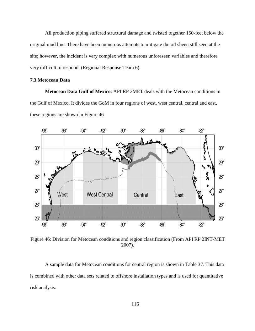
116
All production piping suffered structural damage and twisted together 150-feet below the
original mud line. There have been numerous attempts to mitigate the oil sheen still seen at the
site; however, the incident is very complex with numerous unforeseen variables and therefore
very difficult to respond, (Regional Response Team 6).
7.3 Metocean Data
Metocean Data Gulf of Mexico: API RP 2MET deals with the Metocean conditions in
the Gulf of Mexico. It divides the GoM in four regions of west, west central, central and east,
these regions are shown in Figure 46.
Figure 46: Division for Metocean conditions and region classification (From API RP 2INT-MET
2007).
A sample data for Metocean conditions for central region is shown in Table 37. This data
is combined with other data sets related to offshore installation types and is used for quantitative
risk analysis.
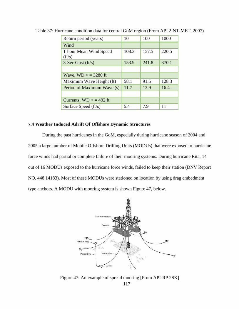
117
Table 37: Hurricane condition data for central GoM region (From API 2INT-MET, 2007)
Return period (years) 10 100 1000
Wind
1-hour Mean Wind Speed
(ft/s)
108.3 157.5 220.5
3-Sec Gust (ft/s) 153.9 241.8 370.1
Wave, WD > = 3280 ft
Maximum Wave Height (ft) 58.1 91.5 128.3
Period of Maximum Wave (s) 11.7 13.9 16.4
Currents, WD > = 492 ft
Surface Speed (ft/s) 5.4 7.9 11
7.4 Weather Induced Adrift Of Offshore Dynamic Structures
During the past hurricanes in the GoM, especially during hurricane season of 2004 and
2005 a large number of Mobile Offshore Drilling Units (MODUs) that were exposed to hurricane
force winds had partial or complete failure of their mooring systems. During hurricane Rita, 14
out of 16 MODUs exposed to the hurricane force winds, failed to keep their station (DNV Report
NO. 448 14183). Most of these MODUs were stationed on location by using drag embedment
type anchors. A MODU with mooring system is shown Figure 47, below.
Figure 47: An example of spread mooring [From API-RP 2SK]
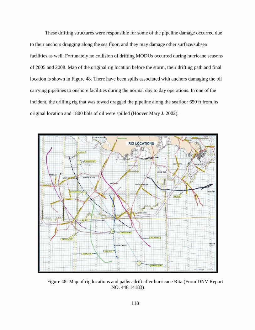
118
These drifting structures were responsible for some of the pipeline damage occurred due
to their anchors dragging along the sea floor, and they may damage other surface/subsea
facilities as well. Fortunately no collision of drifting MODUs occurred during hurricane seasons
of 2005 and 2008. Map of the original rig location before the storm, their drifting path and final
location is shown in Figure 48. There have been spills associated with anchors damaging the oil
carrying pipelines to onshore facilities during the normal day to day operations. In one of the
incident, the drilling rig that was towed dragged the pipeline along the seafloor 650 ft from its
original location and 1800 bbls of oil were spilled (Hoover Mary J. 2002).
Figure 48: Map of rig locations and paths adrift after hurricane Rita (From DNV Report
NO. 448 14183)
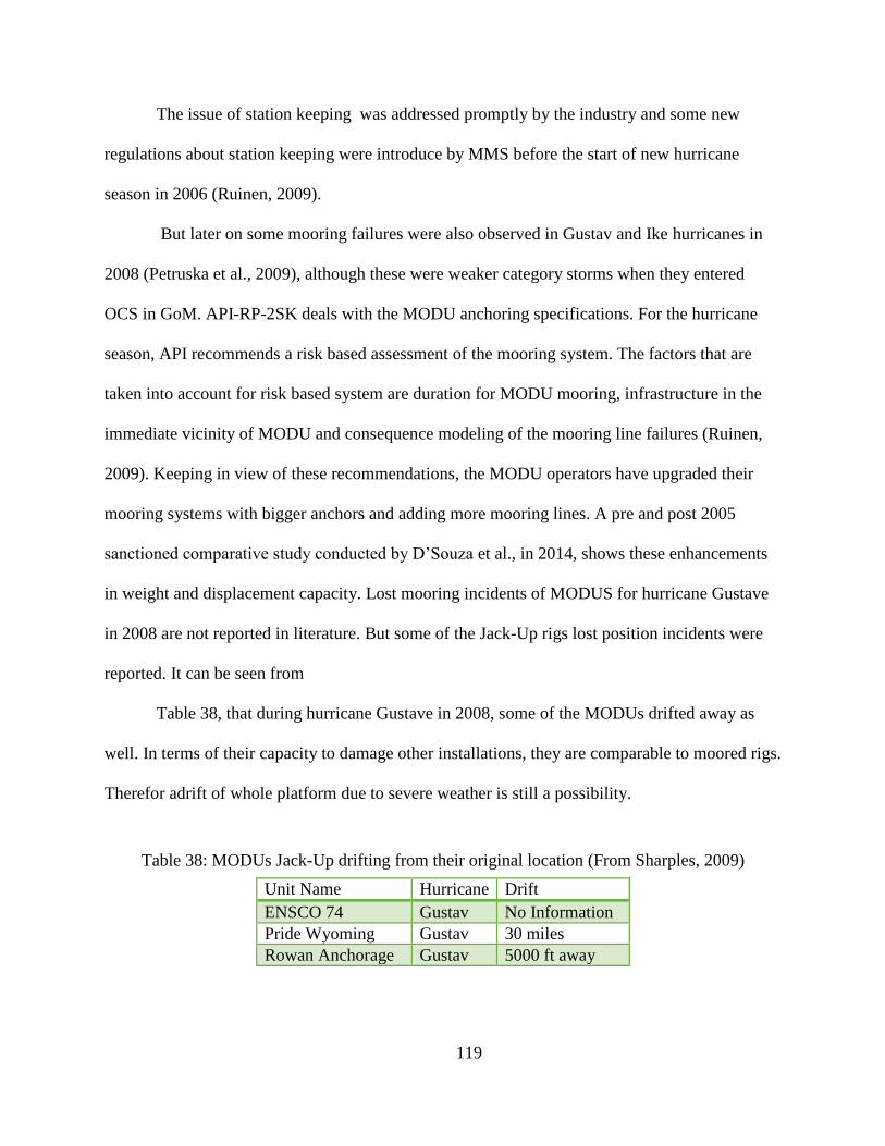
119
The issue of station keeping was addressed promptly by the industry and some new
regulations about station keeping were introduce by MMS before the start of new hurricane
season in 2006 (Ruinen, 2009).
But later on some mooring failures were also observed in Gustav and Ike hurricanes in
2008 (Petruska et al., 2009), although these were weaker category storms when they entered
OCS in GoM. API-RP-2SK deals with the MODU anchoring specifications. For the hurricane
season, API recommends a risk based assessment of the mooring system. The factors that are
taken into account for risk based system are duration for MODU mooring, infrastructure in the
immediate vicinity of MODU and consequence modeling of the mooring line failures (Ruinen,
2009). Keeping in view of these recommendations, the MODU operators have upgraded their
mooring systems with bigger anchors and adding more mooring lines. A pre and post 2005
sanctioned comparative study conducted by D’Souza et al., in 2014, shows these enhancements
in weight and displacement capacity. Lost mooring incidents of MODUS for hurricane Gustave
in 2008 are not reported in literature. But some of the Jack-Up rigs lost position incidents were
reported. It can be seen from
Table 38, that during hurricane Gustave in 2008, some of the MODUs drifted away as
well. In terms of their capacity to damage other installations, they are comparable to moored rigs.
Therefor adrift of whole platform due to severe weather is still a possibility.
Table 38: MODUs Jack-Up drifting from their original location (From Sharples, 2009)
Unit Name Hurricane Drift
ENSCO 74 Gustav No Information
Pride Wyoming Gustav 30 miles
Rowan Anchorage Gustav 5000 ft away
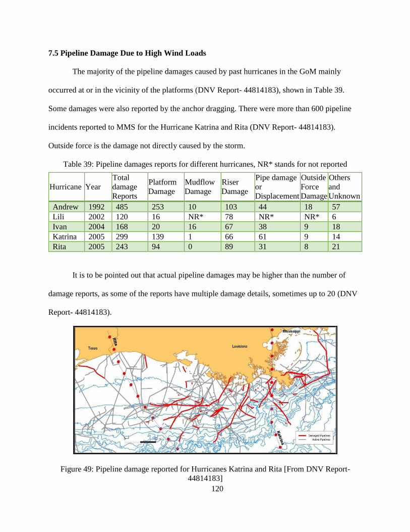
120
7.5 Pipeline Damage Due to High Wind Loads
The majority of the pipeline damages caused by past hurricanes in the GoM mainly
occurred at or in the vicinity of the platforms (DNV Report- 44814183), shown in Table 39.
Some damages were also reported by the anchor dragging. There were more than 600 pipeline
incidents reported to MMS for the Hurricane Katrina and Rita (DNV Report- 44814183).
Outside force is the damage not directly caused by the storm.
Table 39: Pipeline damages reports for different hurricanes, NR* stands for not reported
Hurricane Year
Total
damage
Reports
Platform
Damage
Mudflow
Damage
Riser
Damage
Pipe damage
or
Displacement
Outside
Force
Damage
Others
and
Unknown
Andrew 1992 485 253 10 103 44 18 57
Lili 2002 120 16 NR* 78 NR* NR* 6
Ivan 2004 168 20 16 67 38 9 18
Katrina 2005 299 139 1 66 61 9 14
Rita 2005 243 94 0 89 31 8 21
It is to be pointed out that actual pipeline damages may be higher than the number of
damage reports, as some of the reports have multiple damage details, sometimes up to 20 (DNV
Report- 44814183).
Figure 49: Pipeline damage reported for Hurricanes Katrina and Rita [From DNV Report-
44814183]
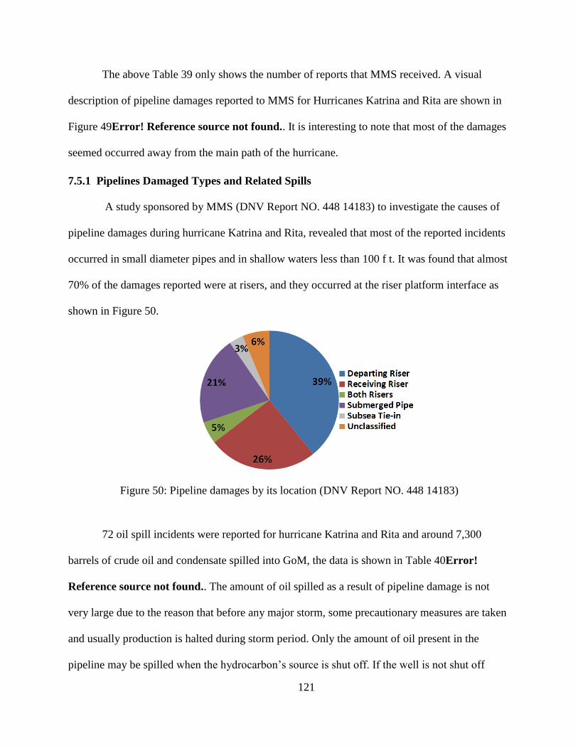
121
The above Table 39 only shows the number of reports that MMS received. A visual
description of pipeline damages reported to MMS for Hurricanes Katrina and Rita are shown in
Figure 49Error! Reference source not found.. It is interesting to note that most of the damages
seemed occurred away from the main path of the hurricane.
7.5.1 Pipelines Damaged Types and Related Spills
A study sponsored by MMS (DNV Report NO. 448 14183) to investigate the causes of
pipeline damages during hurricane Katrina and Rita, revealed that most of the reported incidents
occurred in small diameter pipes and in shallow waters less than 100 f t. It was found that almost
70% of the damages reported were at risers, and they occurred at the riser platform interface as
shown in Figure 50.
Figure 50: Pipeline damages by its location (DNV Report NO. 448 14183)
72 oil spill incidents were reported for hurricane Katrina and Rita and around 7,300
barrels of crude oil and condensate spilled into GoM, the data is shown in Table 40Error!
Reference source not found.. The amount of oil spilled as a result of pipeline damage is not
very large due to the reason that before any major storm, some precautionary measures are taken
and usually production is halted during storm period. Only the amount of oil present in the
pipeline may be spilled when the hydrocarbon’s source is shut off. If the well is not shut off
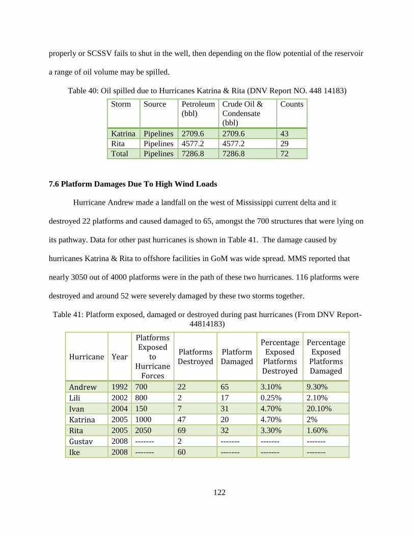
122
properly or SCSSV fails to shut in the well, then depending on the flow potential of the reservoir
a range of oil volume may be spilled.
Table 40: Oil spilled due to Hurricanes Katrina & Rita (DNV Report NO. 448 14183)
Storm Source Petroleum
(bbl)
Crude Oil &
Condensate
(bbl)
Counts
Katrina Pipelines 2709.6 2709.6 43
Rita Pipelines 4577.2 4577.2 29
Total Pipelines 7286.8 7286.8 72
7.6 Platform Damages Due To High Wind Loads
Hurricane Andrew made a landfall on the west of Mississippi current delta and it
destroyed 22 platforms and caused damaged to 65, amongst the 700 structures that were lying on
its pathway. Data for other past hurricanes is shown in Table 41. The damage caused by
hurricanes Katrina & Rita to offshore facilities in GoM was wide spread. MMS reported that
nearly 3050 out of 4000 platforms were in the path of these two hurricanes. 116 platforms were
destroyed and around 52 were severely damaged by these two storms together.
Table 41: Platform exposed, damaged or destroyed during past hurricanes (From DNV Report-
44814183)
Hurricane Year
Platforms Exposed
to Hurricane
Forces
Platforms Destroyed
Platform Damaged
Percentage Exposed
Platforms Destroyed
Percentage Exposed
Platforms Damaged
Andrew 1992 700 22 65 3.10% 9.30%
Lili 2002 800 2 17 0.25% 2.10%
Ivan 2004 150 7 31 4.70% 20.10%
Katrina 2005 1000 47 20 4.70% 2%
Rita 2005 2050 69 32 3.30% 1.60%
Gustav 2008 ------- 2 ------- ------- -------
Ike 2008 ------- 60 ------- ------- -------
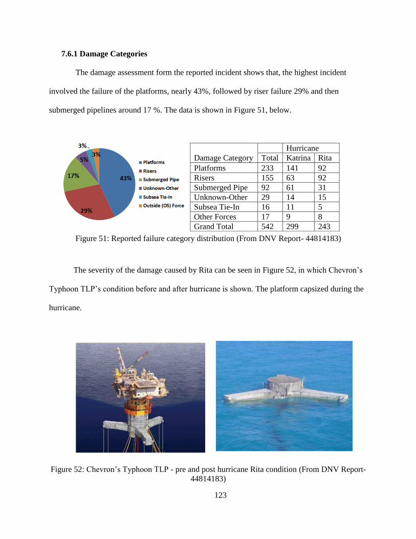
123
7.6.1 Damage Categories
The damage assessment form the reported incident shows that, the highest incident
involved the failure of the platforms, nearly 43%, followed by riser failure 29% and then
submerged pipelines around 17 %. The data is shown in Figure 51, below.
Damage Category
Hurricane
Total Katrina Rita
Platforms 233 141 92
Risers 155 63 92
Submerged Pipe 92 61 31
Unknown-Other 29 14 15
Subsea Tie-In 16 11 5
Other Forces 17 9 8
Grand Total 542 299 243
Figure 51: Reported failure category distribution (From DNV Report- 44814183)
The severity of the damage caused by Rita can be seen in Figure 52, in which Chevron’s
Typhoon TLP’s condition before and after hurricane is shown. The platform capsized during the
hurricane.
Figure 52: Chevron’s Typhoon TLP - pre and post hurricane Rita condition (From DNV Report-
44814183)
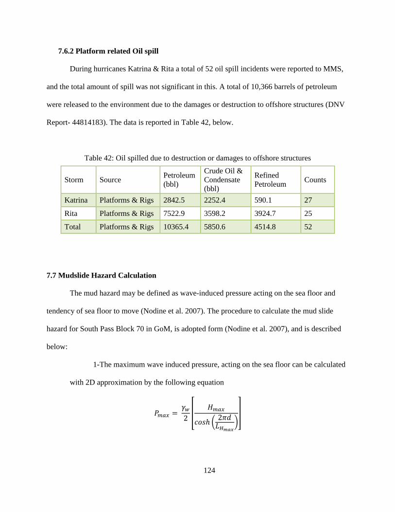
124
7.6.2 Platform related Oil spill
During hurricanes Katrina & Rita a total of 52 oil spill incidents were reported to MMS,
and the total amount of spill was not significant in this. A total of 10,366 barrels of petroleum
were released to the environment due to the damages or destruction to offshore structures (DNV
Report- 44814183). The data is reported in Table 42, below.
Table 42: Oil spilled due to destruction or damages to offshore structures
Storm Source Petroleum
(bbl)
Crude Oil &
Condensate
(bbl)
Refined
Petroleum Counts
Katrina Platforms & Rigs 2842.5 2252.4 590.1 27
Rita Platforms & Rigs 7522.9 3598.2 3924.7 25
Total Platforms & Rigs 10365.4 5850.6 4514.8 52
7.7 Mudslide Hazard Calculation
The mud hazard may be defined as wave-induced pressure acting on the sea floor and
tendency of sea floor to move (Nodine et al. 2007). The procedure to calculate the mud slide
hazard for South Pass Block 70 in GoM, is adopted form (Nodine et al. 2007), and is described
below:
1-The maximum wave induced pressure, acting on the sea floor can be calculated
with 2D approximation by the following equation
𝑃𝑚𝑎𝑥 = 𝛾𝑤
2[
𝐻𝑚𝑎𝑥
𝑐𝑜𝑠ℎ (2𝜋𝑑
𝐿𝐻𝑚𝑎𝑥
)]
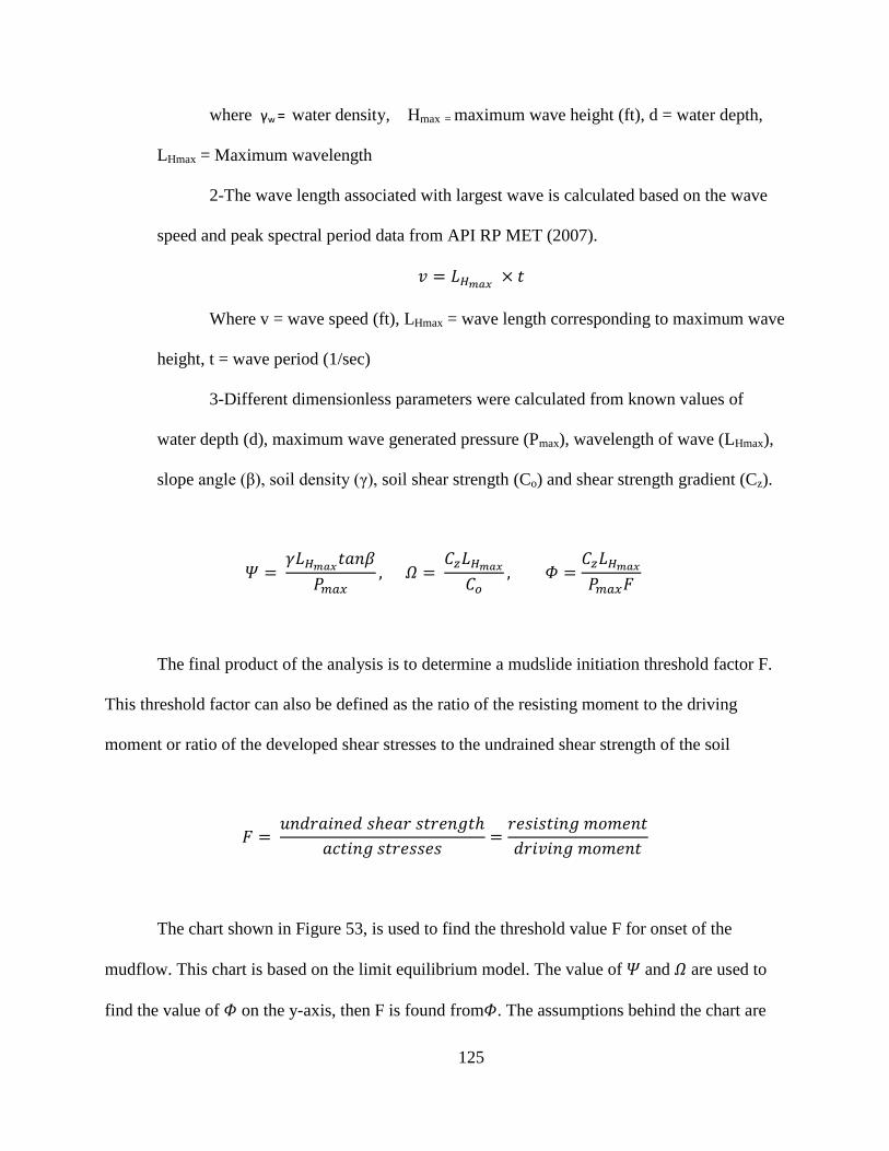
125
where γw = water density, Hmax = maximum wave height (ft), d = water depth,
LHmax = Maximum wavelength
2-The wave length associated with largest wave is calculated based on the wave
speed and peak spectral period data from API RP MET (2007).
𝑣 = 𝐿𝐻𝑚𝑎𝑥 × 𝑡
Where v = wave speed (ft), LHmax = wave length corresponding to maximum wave
height, t = wave period (1/sec)
3-Different dimensionless parameters were calculated from known values of
water depth (d), maximum wave generated pressure (Pmax), wavelength of wave (LHmax),
slope angle (β), soil density (γ), soil shear strength (Co) and shear strength gradient (Cz).
𝛹 = 𝛾𝐿𝐻𝑚𝑎𝑥
𝑡𝑎𝑛𝛽
𝑃𝑚𝑎𝑥, 𝛺 =
𝐶𝑧𝐿𝐻𝑚𝑎𝑥
𝐶𝑜, 𝛷 =
𝐶𝑧𝐿𝐻𝑚𝑎𝑥
𝑃𝑚𝑎𝑥𝐹
The final product of the analysis is to determine a mudslide initiation threshold factor F.
This threshold factor can also be defined as the ratio of the resisting moment to the driving
moment or ratio of the developed shear stresses to the undrained shear strength of the soil
𝐹 = 𝑢𝑛𝑑𝑟𝑎𝑖𝑛𝑒𝑑 𝑠ℎ𝑒𝑎𝑟 𝑠𝑡𝑟𝑒𝑛𝑔𝑡ℎ
𝑎𝑐𝑡𝑖𝑛𝑔 𝑠𝑡𝑟𝑒𝑠𝑠𝑒𝑠=
𝑟𝑒𝑠𝑖𝑠𝑡𝑖𝑛𝑔 𝑚𝑜𝑚𝑒𝑛𝑡
𝑑𝑟𝑖𝑣𝑖𝑛𝑔 𝑚𝑜𝑚𝑒𝑛𝑡
The chart shown in Figure 53, is used to find the threshold value F for onset of the
mudflow. This chart is based on the limit equilibrium model. The value of 𝛹 and 𝛺 are used to
find the value of 𝛷 on the y-axis, then F is found from𝛷. The assumptions behind the chart are
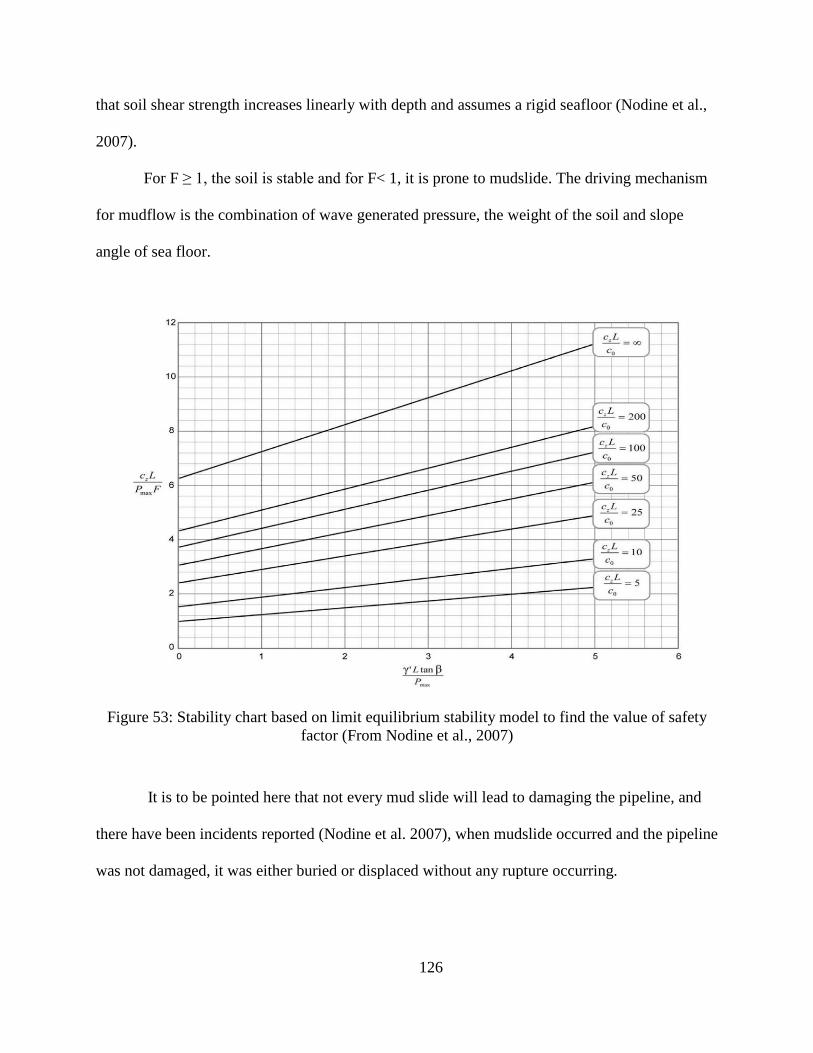
126
that soil shear strength increases linearly with depth and assumes a rigid seafloor (Nodine et al.,
2007).
For F ≥ 1, the soil is stable and for F< 1, it is prone to mudslide. The driving mechanism
for mudflow is the combination of wave generated pressure, the weight of the soil and slope
angle of sea floor.
Figure 53: Stability chart based on limit equilibrium stability model to find the value of safety
factor (From Nodine et al., 2007)
It is to be pointed here that not every mud slide will lead to damaging the pipeline, and
there have been incidents reported (Nodine et al. 2007), when mudslide occurred and the pipeline
was not damaged, it was either buried or displaced without any rupture occurring.
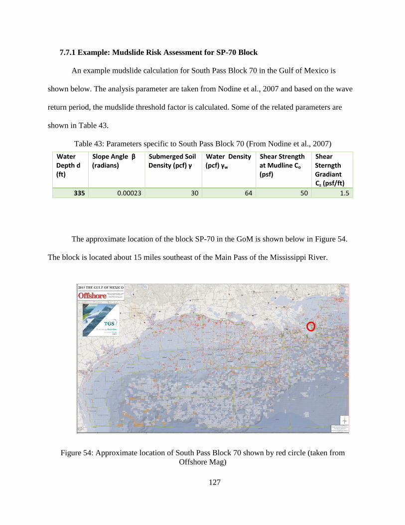
127
7.7.1 Example: Mudslide Risk Assessment for SP-70 Block
An example mudslide calculation for South Pass Block 70 in the Gulf of Mexico is
shown below. The analysis parameter are taken from Nodine et al., 2007 and based on the wave
return period, the mudslide threshold factor is calculated. Some of the related parameters are
shown in Table 43.
Table 43: Parameters specific to South Pass Block 70 (From Nodine et al., 2007)
Water Depth d (ft)
Slope Angle β (radians)
Submerged Soil Density (pcf) γ
Water Density (pcf) γw
Shear Strength at Mudline Co (psf)
Shear Sterngth Gradiant Cz (psf/ft)
335 0.00023 30 64 50 1.5
The approximate location of the block SP-70 in the GoM is shown below in Figure 54.
The block is located about 15 miles southeast of the Main Pass of the Mississippi River.
Figure 54: Approximate location of South Pass Block 70 shown by red circle (taken from
Offshore Mag)
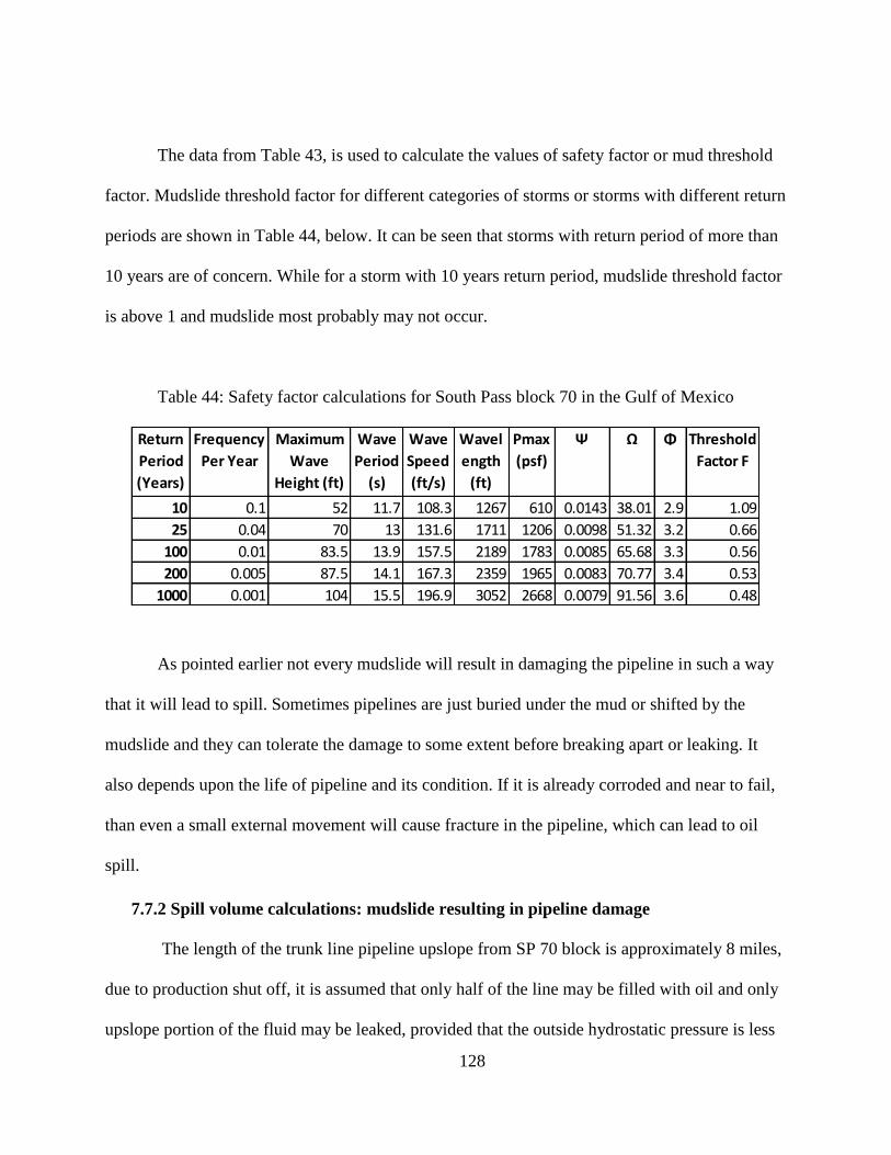
128
The data from Table 43, is used to calculate the values of safety factor or mud threshold
factor. Mudslide threshold factor for different categories of storms or storms with different return
periods are shown in Table 44, below. It can be seen that storms with return period of more than
10 years are of concern. While for a storm with 10 years return period, mudslide threshold factor
is above 1 and mudslide most probably may not occur.
Table 44: Safety factor calculations for South Pass block 70 in the Gulf of Mexico
As pointed earlier not every mudslide will result in damaging the pipeline in such a way
that it will lead to spill. Sometimes pipelines are just buried under the mud or shifted by the
mudslide and they can tolerate the damage to some extent before breaking apart or leaking. It
also depends upon the life of pipeline and its condition. If it is already corroded and near to fail,
than even a small external movement will cause fracture in the pipeline, which can lead to oil
spill.
7.7.2 Spill volume calculations: mudslide resulting in pipeline damage
The length of the trunk line pipeline upslope from SP 70 block is approximately 8 miles,
due to production shut off, it is assumed that only half of the line may be filled with oil and only
upslope portion of the fluid may be leaked, provided that the outside hydrostatic pressure is less
Return
Period
(Years)
Frequency
Per Year
Maximum
Wave
Height (ft)
Wave
Period
(s)
Wave
Speed
(ft/s)
Wavel
ength
(ft)
Pmax
(psf)
Ψ Ω Φ Threshold
Factor F
10 0.1 52 11.7 108.3 1267 610 0.0143 38.01 2.9 1.09
25 0.04 70 13 131.6 1711 1206 0.0098 51.32 3.2 0.66
100 0.01 83.5 13.9 157.5 2189 1783 0.0085 65.68 3.3 0.56
200 0.005 87.5 14.1 167.3 2359 1965 0.0083 70.77 3.4 0.53
1000 0.001 104 15.5 196.9 3052 2668 0.0079 91.56 3.6 0.48
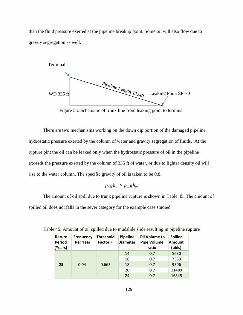
129
than the fluid pressure exerted at the pipeline breakup point. Some oil will also flow due to
gravity segregation as well.
There are two mechanisms working on the down dip portion of the damaged pipeline,
hydrostatic pressure exerted by the column of water and gravity segregation of fluids. At the
rupture pint the oil can be leaked only when the hydrostatic pressure of oil in the pipeline
exceeds the pressure exerted by the column of 335 ft of water, or due to lighter density oil will
rise to the water column. The specific gravity of oil is taken to be 0.8.
𝜌𝑜𝑔ℎ𝑜 ≥ 𝜌𝑤𝑔ℎ𝑤
The amount of oil spill due to trunk pipeline rupture is shown in Table 45. The amount of
spilled oil does not falls in the sever category for the example case studied.
Table 45: Amount of oil spilled due to mudslide slide resulting in pipeline rupture
Return Period (Years)
Frequency Per Year
Threshold Factor F
Pipeline Diameter
Oil Volume to Pipe Volume
ratio
Spilled Amount
(bbls)
25 0.04 0.663
14 0.7 5630
16 0.7 7353
18 0.7 9306
20 0.7 11489
24 0.7 16545
Terminal
WD 335 ft Leaking Point SP-70
Figure 55: Schematic of trunk line from leaking point to terminal
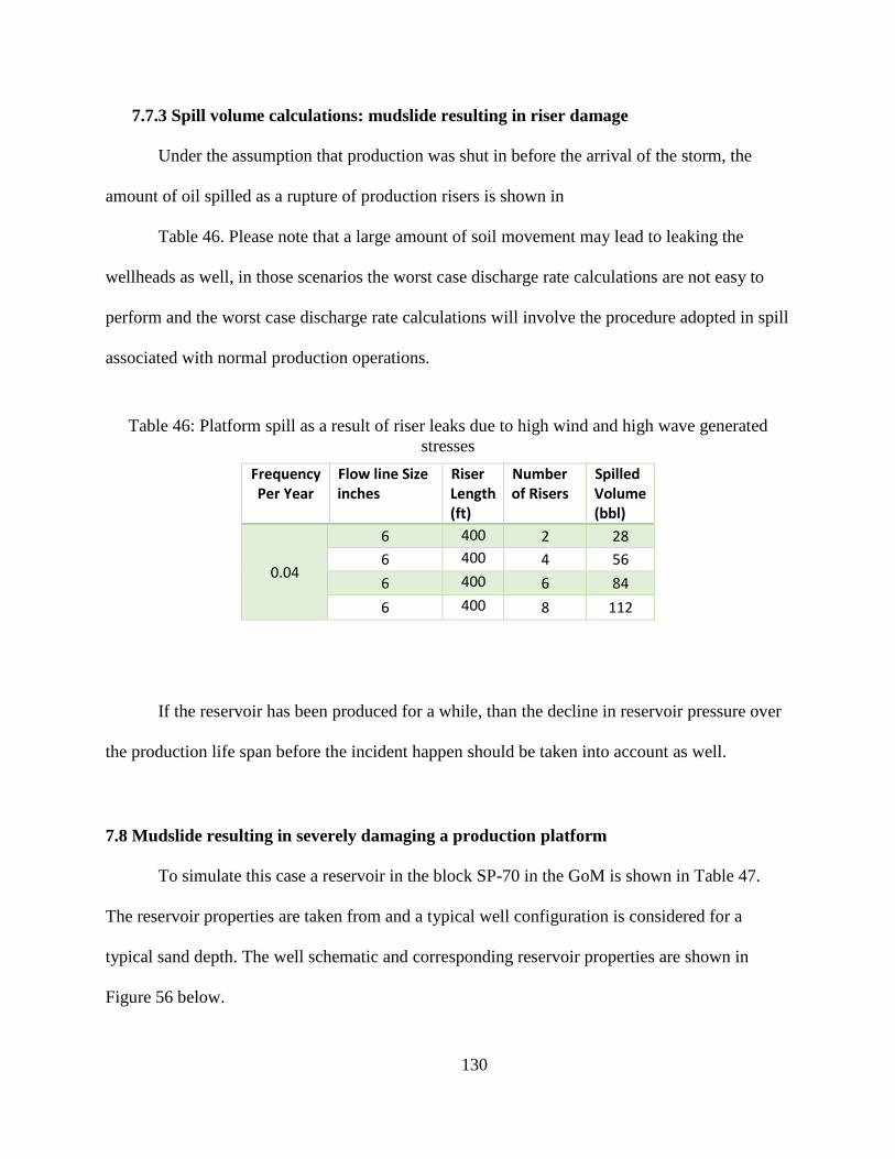
130
7.7.3 Spill volume calculations: mudslide resulting in riser damage
Under the assumption that production was shut in before the arrival of the storm, the
amount of oil spilled as a rupture of production risers is shown in
Table 46. Please note that a large amount of soil movement may lead to leaking the
wellheads as well, in those scenarios the worst case discharge rate calculations are not easy to
perform and the worst case discharge rate calculations will involve the procedure adopted in spill
associated with normal production operations.
Table 46: Platform spill as a result of riser leaks due to high wind and high wave generated
stresses
Frequency Per Year
Flow line Size inches
Riser Length (ft)
Number of Risers
Spilled Volume (bbl)
0.04
6 400 2 28
6 400 4 56
6 400 6 84
6 400 8 112
If the reservoir has been produced for a while, than the decline in reservoir pressure over
the production life span before the incident happen should be taken into account as well.
7.8 Mudslide resulting in severely damaging a production platform
To simulate this case a reservoir in the block SP-70 in the GoM is shown in Table 47.
The reservoir properties are taken from and a typical well configuration is considered for a
typical sand depth. The well schematic and corresponding reservoir properties are shown in
Figure 56 below.
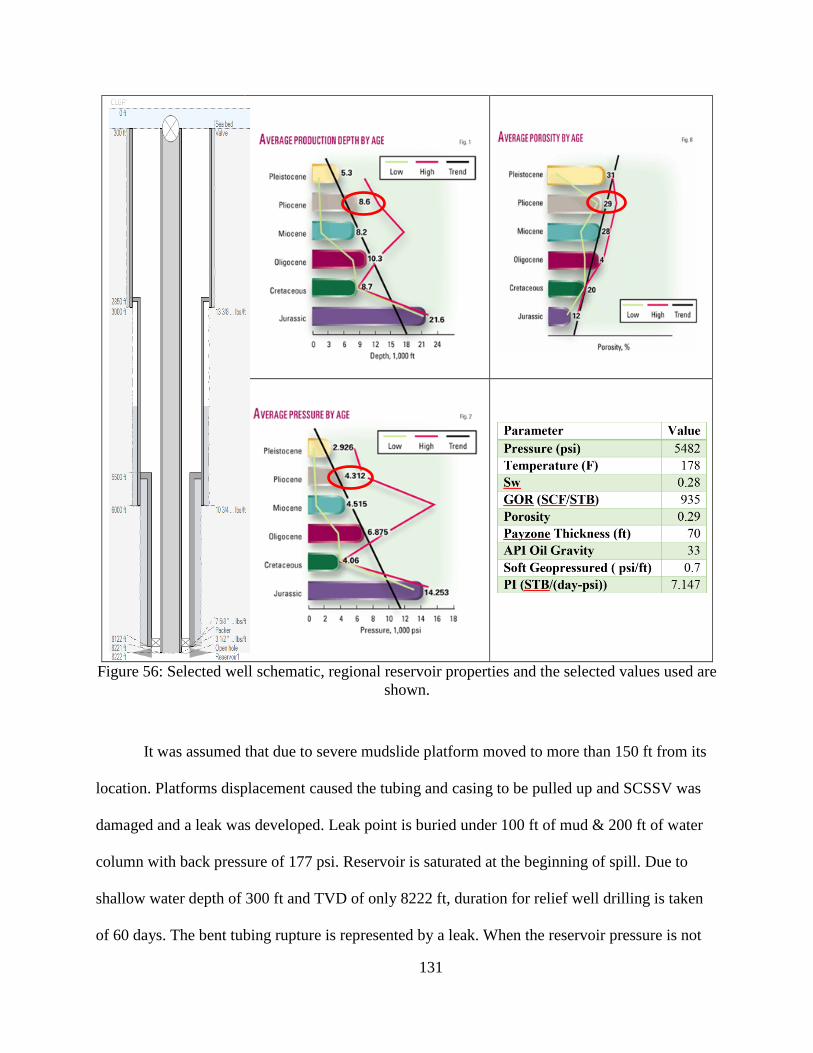
131
Figure 56: Selected well schematic, regional reservoir properties and the selected values used are
shown.
It was assumed that due to severe mudslide platform moved to more than 150 ft from its
location. Platforms displacement caused the tubing and casing to be pulled up and SCSSV was
damaged and a leak was developed. Leak point is buried under 100 ft of mud & 200 ft of water
column with back pressure of 177 psi. Reservoir is saturated at the beginning of spill. Due to
shallow water depth of 300 ft and TVD of only 8222 ft, duration for relief well drilling is taken
of 60 days. The bent tubing rupture is represented by a leak. When the reservoir pressure is not
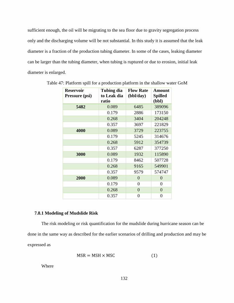
132
sufficient enough, the oil will be migrating to the sea floor due to gravity segregation process
only and the discharging volume will be not substantial. In this study it is assumed that the leak
diameter is a fraction of the production tubing diameter. In some of the cases, leaking diameter
can be larger than the tubing diameter, when tubing is ruptured or due to erosion, initial leak
diameter is enlarged.
Table 47: Platform spill for a production platform in the shallow water GoM
Reservoir
Pressure (psi)
Tubing dia
to Leak dia
ratio
Flow Rate
(bbl/day)
Amount
Spilled
(bbl)
5482 0.089 6485 389096
0.179 2886 173150
0.268 3404 204248
0.357 3697 221829
4000 0.089 3729 223755
0.179 5245 314676
0.268 5912 354739
0.357 6287 377250
3000 0.089 1932 115890
0.179 8462 507728
0.268 9165 549901
0.357 9579 574747
2000 0.089 0 0
0.179 0 0
0.268 0 0
0.357 0 0
7.8.1 Modeling of Mudslide Risk
The risk modeling or risk quantification for the mudslide during hurricane season can be
done in the same way as described for the earlier scenarios of drilling and production and may be
expressed as
MSR = MSH × MSC (1)
Where
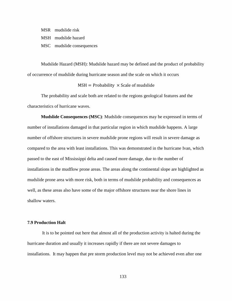
133
MSR mudslide risk
MSH mudslide hazard
MSC mudslide consequences
Mudslide Hazard (MSH): Mudslide hazard may be defined and the product of probability
of occurrence of mudslide during hurricane season and the scale on which it occurs
MSH = Probability × Scale of mudslide
The probability and scale both are related to the regions geological features and the
characteristics of hurricane waves.
Mudslide Consequences (MSC): Mudslide consequences may be expressed in terms of
number of installations damaged in that particular region in which mudslide happens. A large
number of offshore structures in severe mudslide prone regions will result in severe damage as
compared to the area with least installations. This was demonstrated in the hurricane Ivan, which
passed to the east of Mississippi delta and caused more damage, due to the number of
installations in the mudflow prone areas. The areas along the continental slope are highlighted as
mudslide prone area with more risk, both in terms of mudslide probability and consequences as
well, as these areas also have some of the major offshore structures near the shore lines in
shallow waters.
7.9 Production Halt
It is to be pointed out here that almost all of the production activity is halted during the
hurricane duration and usually it increases rapidly if there are not severe damages to
installations. It may happen that pre storm production level may not be achieved even after one
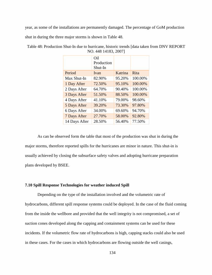
134
year, as some of the installations are permanently damaged. The percentage of GoM production
shut in during the three major storms is shown in Table 48.
Table 48: Production Shut-In due to hurricane, historic trends [data taken from DNV REPORT
NO. 448 14183, 2007]
Oil
Production
Shut-In
Period Ivan Katrina Rita
Max Shut-In 82.90% 95.20% 100.00%
1 Day After 72.50% 95.10% 100.00%
2 Days After 64.70% 90.40% 100.00%
3 Days After 51.50% 88.50% 100.00%
4 Days After 41.10% 79.00% 98.60%
5 Days After 39.20% 73.30% 97.80%
6 Days After 34.00% 69.60% 94.70%
7 Days After 27.70% 58.00% 92.80%
14 Days After 28.50% 56.40% 77.50%
As can be observed form the table that most of the production was shut in during the
major storms, therefore reported spills for the hurricanes are minor in nature. This shut-in is
usually achieved by closing the subsurface safety valves and adopting hurricane preparation
plans developed by BSEE.
7.10 Spill Response Technologies for weather induced Spill
Depending on the type of the installation involved and the volumetric rate of
hydrocarbons, different spill response systems could be deployed. In the case of the fluid coming
from the inside the wellbore and provided that the well integrity is not compromised, a set of
suction cones developed along the capping and containment systems can be used for these
incidents. If the volumetric flow rate of hydrocarbons is high, capping stacks could also be used
in these cases. For the cases in which hydrocarbons are flowing outside the well casings,
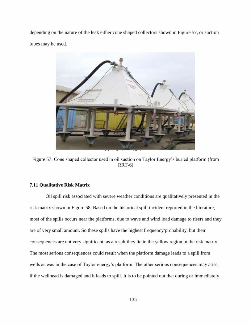
135
depending on the nature of the leak either cone shaped collectors shown in Figure 57, or suction
tubes may be used.
Figure 57: Cone shaped collector used in oil suction on Taylor Energy’s buried platform (from
RRT-6)
7.11 Qualitative Risk Matrix
Oil spill risk associated with severe weather conditions are qualitatively presented in the
risk matrix shown in Figure 58. Based on the historical spill incident reported in the literature,
most of the spills occurs near the platforms, due to wave and wind load damage to risers and they
are of very small amount. So these spills have the highest frequency/probability, but their
consequences are not very significant, as a result they lie in the yellow region in the risk matrix.
The most serious consequences could result when the platform damage leads to a spill from
wells as was in the case of Taylor energy’s platform. The other serious consequences may arise,
if the wellhead is damaged and it leads to spill. It is to be pointed out that during or immediately
136
after the storm, due to problems in mobilization of the response systems, a blowing well may
result in very serious consequence.
Figure 58: Qualitatively risk matrix for spills due to severe weather conditions
7.12 Conclusions and Observations
GoM is prone to hurricanes ranging from category 1 to category 5 and in the recent past
severe damage to pipelines and platforms has been reported, and there is always the
possibility of a spill resulting from either pipeline or platform structural damage.
Severe weather may also result in drifting of floating offshore structures, especially
MODUs. These drifting structures may pose threat to other offshore facilities. Their
High Risk
Moderate
Risk
Low Risk
137
collision with other platforms or their anchors dragging along the sea floor may result in
severely damaging subsea installations and may lead to a spill.
A sample analysis perfomed in this study and past huuricane related spill data shows
that most of the spills associated with severe weather will be of small amount, as most of
the drilling/production operations are stopped before arrival of the storm.
According to oil industry’s standard procedure for hurricane, all of the production in the
expected path of the hurricane is shut down and offshore facilities are evacuated.
Therefore damage to pipeline or platform will not lead to a large spill.
In shallow waters of up to 400 ft in current or old Mississippi river delta, the mudflow
caused by high wave surge phenomenon is the biggest hazard for offshore installations.
This mudslide may lead to a very complex situation in which it may become difficult to
estimate the WCD rate or deploy the proper response system to stop the spill. The burial
of Tylor’s energy’s platform is such an example.
The South Pass block SP-70 in the current Mississippi river delta was selected to conduct
the mudslide quantitative risk assessment. An example calculation has been performed
for mudslide resulting in pipeline and platform damage and resultant spill amount.
Aanalysis shows that a storm with return period of 10 years may trigger the mudslide in
South Pass-70 block, which may lead to offshore faicilties damage.
Historical data trend shows that most of the spills reportde for past hurricane, occured in
the vicinity of the platforms due to riser damage. The sample caluculation performed
show an oil spill of 112 bbls only, in the case that risers are damaged in the vivinity of
hypothetical platform in SP-70 block. Amongest the weather related spills, rsiser spills
are most frequent but least harmfull in terms of spill amount.
138
A worst case discharge rate of 6485 BOPD was estimated by selecting representative
well and reservoir properties corresponding to a hypothetical production platform in the
SP-70 block, when mudslide results in complete burial of the platform.
The deployment of response system in this case becomes very difficult, due to difficulty
in exactly pointing out the source location. Some type of marking/coating on the
conductor casing are suggested, which may be useful in this type of burial scenario to
identify the location of the souce.
Adrift of floating structures is still a hazard, even after stringent regulatory requirements
for fastening these systems. The drifting structure can damage other installations on sea
surface or subsea and can result in very small to large oil spills.
Spill response systems for the weather related incidents needs enhancements, especillay
collection domes/cones that are usually used in response to such events have not proven
very useful in past.
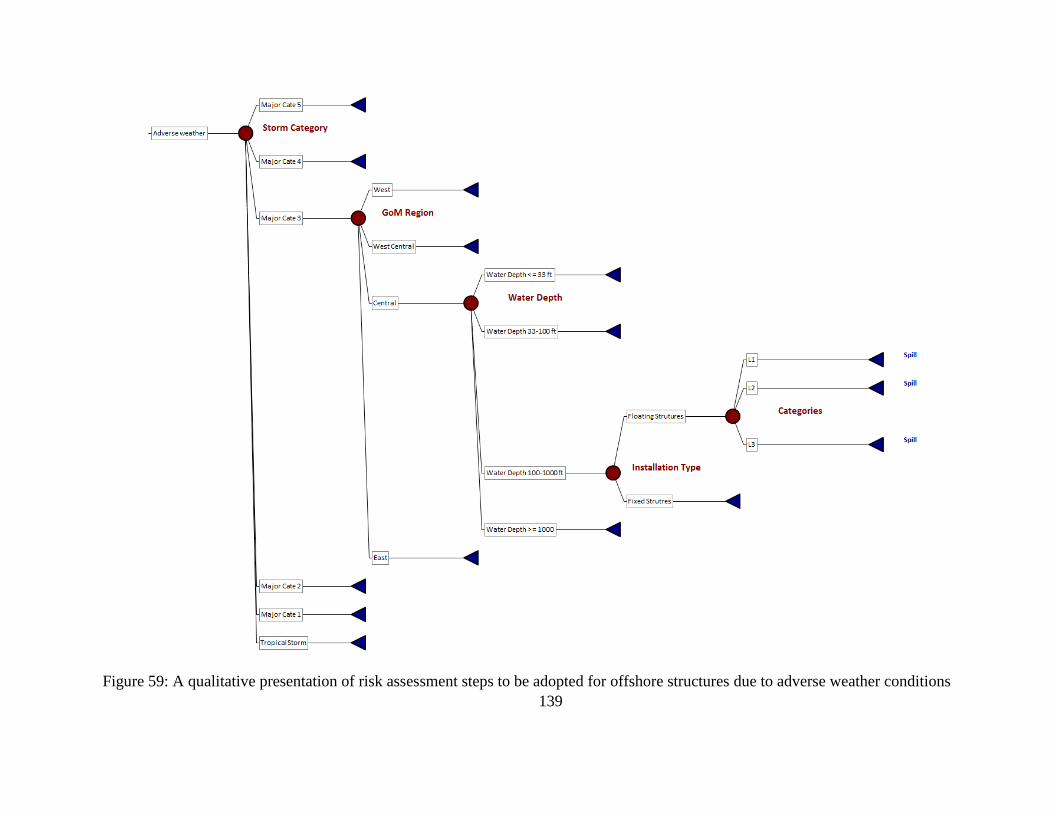
139
Figure 59: A qualitative presentation of risk assessment steps to be adopted for offshore structures due to adverse weather conditions
140
CHAPTER 8: CONCLUDING REMARKS AND FUTURE DIRECTIONS
Concluding remarks for all of five oil spill scenarios modeled in this study are given
below.
8.1 Scenario-1: Exploratory Well
An example of quantitative risk assessment (QRA) for deepwater exploratory drilling well
blowout is presented, QRA facilitated in better understanding of blowout risks.
The selection of a specific well and corresponding reservoir properties and taking into
account the regional variation in reservoir properties by fitting lognormal/triangular
distributions and conducting Monte Carlo simulations, provided a realistic representation of
the reservoir properties to calculate the worst case discharge rates.
Unexpected pore pressure, delayed response to an incident and failure to detect the error
were found to be three most important basic events contributing to the overall risk of the
system. These were identified by conducting Fussell Vesely (FV) importance analysis.
The FV importance analysis emphasize the need to focus on the technologies to provide
early warnings for unexpected pore pressure during drilling phase, eliminating the delays
that can occur when responding to an emergency situation by automation of some of the
decision processes and technologically improve the reliability of sensors that detect an
error. Crew training and management is also an important element in responding to
situations that needs immediate attention.
The worst case discharge rate of nearly 104,000 BOPD was estimated for the case when
drill pipe is out of the hole and BOP offers no restriction to blowing hydrocarbons
141
(conditions specified by BSEE to estimate WCD). The occurrence of this combination of
events is amongst the least probable situations. Therefore risk which is a product of
probability and spilled oil volume is not very high in this case.
The 100,000 BOPD oil handling capacity of newly built capping and containment systems
is nearly sufficient to either capture or contain the computed worst case discharge oil rate
of 104,000 BPD.
The reservoir pressure drop and resultant reduction in flow rate are not significant in the
cases when the fluids are flowing either through drillpipe-casing annulus or through drill
pipe.
The selection of the multiphase correlation also affects the worst case discharge rate
estimates and computed values with some other correlation may differ from the values
computed in this study, therefore this variation in values must be considered when making
decision based on the WCD rates.
Restrictions in the flow path substantially decrease the fluid flow rate and in some of the
circumstances may even choke the flow.
Newly built response systems are effective in reducing the risk of large oil spill in
deepwaters environments, provided that they function properly when they are deployed.
Capping and containment systems are effectives for only one type of failure mode i.e.,
when the flow is coming through the well, which is the most probable scenario based on
the historical blowout data.
Addition of intervention module in capping and containment systems will enhance their
capabilities to deal with other failure modes as well. For example dynamic kill may be used
in the case of an underground blowout.
142
In the case of a blowing well affecting nearby wells, the situation may become complex
and would require additional modules to be added with capping and containment systems
or invoke other response systems.
8.2 Scenario-2: Underground Blowout
The consequences of an underground blowout range from no visible damage at the sea
surface to the loss of the whole rig. It is difficult to quantitatively estimate the risk due to
the involvement of large number of uncertain parameters.
The potential of hydrocarbons leaking to sea floor is a combination of geological settings,
the transmissibility of the paths allowing hydrocarbons to reach sea floor, the pressure of
source reservoir and its potential to create fractures in the low lying geological barriers.
The formulas used to estimate the fault permeability and thickness are very simple and
large uncertainty exists in the estimated parameters of fault permeability and its thickness.
The simulation result show that for low permeability k=0.004 mD fault, that connects a
deep over pressured zone to a shallower low pressure zone, the time taken to recharge the
shallower zone to reach its LOT pressure value is more than 100 years.
A high permeable faulted zone of 40 mD will take 135 years to recharge the low pressure
shallower zone to its LOT pressure value.
In the reservoir model adopted in this scenario, when the ratio of the volume of shallower
to deeper zone decrease to 0.1, the recharging time significantly drops to 24 years only.
Therefore ratio of the two zones is also an important parameter alongside their pressure
differential and the transmissibility of the connecting zone.
143
The worst conditions may occur when the hydrocarbons travel through the casing-wellbore
annulus and may either reach to shallowest zones lying very close to mud line or leak
outside of the well. The casing-wellbore annulus path may have very high permeability due
to fractured cement and/or due to micro annulus gaps in this path. In this case the
hydrocarbons may appear at the sea floor during the drilling activity.
8.3 Scenario-3: Production Well
The QRA study of a deepwater production well has been performed and key contributors
to overall system safety have been identified through fault tree analysis.
Sensitivity analysis of all of the basic events in the constructed Fault Tree for a sand
screen failure leading to blowout was conducted. It turned out to that the three most
important basic events contributing to the frequency of blowout are sand screen failures,
subsea production tree’s control system failure and well control/other failures.
It has been suggested by other researchers that the design improvements of the sand screen
will greatly reduce their failure rates and in turn blowout frequency associated with
production well, as it is one of the most sensitive/important basic event in the system
setup, considered for this scenario.
Subsea production tree’s control system is the second most important basic event in the
system, and even a small improvement in the reliability of control system will greatly
influence the blowout frequency of the entire system.
Monte Carlo simulation results for blowout probability show a range of values between
1.54-2.0 ×10⁻⁵
per well-year, when each of the basic events is varied by ±10%.
144
A WCD rate of 34,546 BOPD was estimated using multiphase fluid simulations and it is
well within the fluid handling capacity of newly built response systems called capping and
containment systems. Newly built response systems are effective in reducing the risk of
large oil spill in deepwater environments. Additional tools like adopter spools may be
needed to connect capping stack to subsea trees with different connector profiles.
The blowout frequency modeled by FTA is based on the historical data and therefore it is a
conservative estimate. When recent technological improvements are incorporated into
FTA, the blowout frequency will be reduced, as in the past few years there have been
major improvements in well safety related procedures. New regulatory requirements,
equipment reliability improvements and extensive training of crew, all of these will
contribute in lowering the blowout frequency estimates.
8.4 Scenario-4: FPSO
The deployment of FPSO for hydrocarbon production in GoM has some advantages and
some related issues that must be taken care of.
The proposed FPSO configuration for the GoM has been analyzed and associated risks
are qualitatively and quantitatively presented.
It has been reported by previous researchers that risk associated with FPSO deployment
in the GoM are comparable to other production platforms and FPSO needs additional
considerations due to its large fluid storage capacity, station keeping requirements and oil
transportation mechanism.
Most of the historical oil spills associated with FPSOs operations actually happened
during oil transportation from FPSO to onshore facilities by shuttle tankers.
145
Reported oil spill incidents involving FPSO vessel are mainly due to loss of its position
keeping and during fuel offloading process. These spills are of very small quantity as
compared to shuttle tanker spills.
An example calculation based on the proposed configuration of FPSO for GoM has been
performed to estimate the frequency of shuttle tanker collision with the FPSO and related
spill amount.
Analysis shows that only small amount 100-200 bbl of oil spills will result due to shuttle
collision with other vessels including FPSO, and maximum spill amount will result when
the shuttle tanker capsizes while carrying hydrocarbons from FPSO to onshore facilities.
The probability of FPSO capsizing is very low, as there are no reported incidents. But if it
is the case, a large oil spill will most probably be expected due to its large fluid storage
capacity and other possible damages that can occur to wellheads or subsea installations.
Amongst the spill response technology, oil skimmers boats seem to be the most
appropriate for spills involving shuttle tankers as these are the most frequent spills
involving production from FPSO.
8.5 Scenario-5: Weather Induced Spills
GoM is prone to hurricanes ranging from category 1 to category 5 and in the recent past
severe damage to pipelines and platforms has been reported, and there is always the
possibility of a spill resulting from either pipeline or platform structural damage.
Severe weather may also result in drifting of floating offshore structures, especially
MODUs. These drifting structures may pose threat to other offshore facilities. Their
146
collision with other platforms or their anchors dragging along the sea floor may result in
severely damaging subsea installations and may lead to a spill.
A sample analysis perfomed in this study and past huuricane related spill data shows that
most of the spills associated with severe weather will be of small amount, as most of the
drilling/production operations are stopped before arrival of the storm.
According to oil industry’s standard procedure for hurricane, all of the production in the
expected path of the hurricane is shut down and offshore facilities are evacuated.
Therefore damage to pipeline or platform will not lead to a large spill.
In shallow waters of up to 400 ft. in current or old Mississippi river delta, the mudflow
caused by high wave surge phenomenon is the biggest hazard for offshore installations.
This mudslide may lead to a very complex situation in which it may become difficult to
estimate the WCD rate or deploy the proper response system to stop the spill. The burial
of Taylor energy platform is such an example.
The South Pass block SP-70 in the current Mississippi river delta was selected to conduct
the mudslide quantitative risk assessment. An example calculation has been performed
for mudslide resulting in pipeline and platform damage and resultant spill amount.
Aanalysis shows that a storm with return period of 10 years may trigger the mudslide in
South Pass-70 block, which may lead to offshore faicilties damage.
Historical data trend shows that most of the spills reportde for past hurricane, occured in
the vicinity of the platforms due to riser damage. The sample caluculation performed
show an oil spill of 112 bbls only, in the case that risers are damaged in the vivinity of
hypothetical platform in SP-70 block. Amongest the weather related spills, rsiser spills
are most frequent but least harmfull in terms of spill amount.
147
A worst case discharge rate of 6485 BOPD was estimated by selecting representative
well and reservoir properties corresponding to a hypothetical production platform in the
SP-70 block, when mudslide results in complete burial of the platform.
The deployment of response system in this case becomes very difficult, due to difficulty
in exactly pointing out the source location. Some type of marking/coating on the
conductor casing are suggested, which may be useful in this type of burial scenario to
identify the location of the souce.
Adrift of floating structures is still a hazard, even after stringent regulatory requirements
for fastening these systems. The drifting structure can damage other installations on sea
surface or subsea and can result in very small to large oil spills.
Spill response systems for the weather related incidents needs enhancements, especillay
collection domes/cones that are usually used in response to such events have not proven
very useful in past.
8.6 Approximations and Limitations
The following are the approximations and limitations of this study
When conclusions have to be made based on the worst case discharge rates, the
uncertainty/variation in the regional reservoir properties used to estimate the WCD
should be considered as well. Therefore instead of a single value for WCD, a range of
values will most probably justify the underlying assumptions.
In estimating WCD, wellbore walls were considered as smooth as having uniform
circular shape. This condition may not hold well in all the cases and addition of
148
roughness of wellbore walls due to mud cake or irregular shape of the wellbore due to
drilling may lead to either low or raise the WCD estimates.
Multiphase fluid flow correlations used to estimate WCD have their own uncertainties,
due to underlying assumptions/simplification in developing these steady state models.
The WCD estimate may differ amongst different multiphase fluid flow models.
The component failure data available to author and used for production scenario is not the
most updated data set available to large offshore operators. The data used set includes
offshore reliability data up to 2001, and there has been a lot of offshore activities between
2001 and now. Therefore including the latest data will improve the accuracy of results.
The BOP and production tree were modeled as a single component, and were not
resolved into network of rams/valves and chokes. A detailed model by using the recent
component data will definitely improve the reliability or failure rate prediction of these
systems.
8.7 Future Directions
The study has the potential to expand in many dimensions; some of them are pointed
here. Most of these can only be performed with access to extensive current data sets available
and may need team work as well.
For the exploratory drilling scenario, the failure rate of risers may be included in the
analysis, that will incorporate the systems above BOP and whole drilling system may be
analyzed including the type of rig.
149
The subsea production filed analysis is another area that warrants attention and the entire
production system can be modeled, starting form reservoir and terminating at the
production facility.
The GoM lease block may be taken as bases for a comprehensive weather induced risk
analysis and a model database may be generated. The input parameters could be the
locations and type of the offshore facility. The output may be a report including the entire
hazards associated with that particular location and facility type under various scenarios
of severe weather.
The component failure data used in constructing the fault tree can be used to carry out the
system reliability analysis as well. The systems may be represented as series or parallel
combination and their mean time before the failure can be found. This may be very useful
for economic analysis and downtime calculations, to estimate the cost associated with
different delays.
150
REFERENCES
@Risk: Risk Analysis and Monte Carlo Simulation Software. http://www.palisade.com/risk/
ACONA, (2012) “Blowout Risk Evaluation in the Labrador Sea SOUTH-WEST OF
GREENLAND, Technical Report, Revision No. 2.3.
http://dce.au.dk/fileadmin/dce.au.dk/Udgivelser/Appendix_2_Blowout_risk_in_the_Labrador_Se
a.pdf
Anderson Cheryl McMahon, Mayes Melinda, and LaBelle Robert (June, 2012), Update of
Occurrence Rates for Offshore Oil Spills, Bureau of Ocean Energy Management, OCS Report
BOEM 2012-069.
API RP 2SK. (2005). Design and Analysis of Stationkeeping Systems for Floating Structures,
American Petroleum Institute.
http://www.api.org/~/media/files/news/hurricane/2sk_add.pdf?la=en
API RP BULLETIN 2INT-MET. (2007). Interim Guidance on Hurricane Conditions in the Gulf
of Mexico. American Petroleum Institute. https://law.resource.org/pub/us/cfr/ibr/002/api.2int-
met.2007.pdf
Bercha, Frank G. (2013) “Updates To Fault Tree For Oil Spill Occurrence Estimators Update Of
GoM And PAC OCS Statistics To 2012”. Final Task 2 Report, OCS Study BOEM 2013-0116.
http://www.boem.gov/2013-0116/
Bruno, M. S. (1992, June 1). Subsidence-Induced Well Failure. Society of Petroleum Engineers.
doi:10.2118/20058-PA.
Busch, J. M. (1985, October 1). Subsurface Safety Valves: Safety Asset or Safety Liability?
Society of Petroleum Engineers. doi:10.2118/12193-PA
Capderou, C., & DiLorenzo, N. R. (2012, January 1). A Fresh Look at Completion Reliability
Supports Sand Control Selection. Society of Petroleum Engineers. doi:10.2118/159541-MS
Chen Haibo (2003), “Probabilistic Evaluations of FPSO-Tanker Collision in Tandem Offloading
Operations”. Norwegian University of Science and Technology
Cook Ann E., Goldberg Dave, Kleinberg Robert L. (2008). Fracture-controlled gas hydrate
systems in the northern Gulf of Mexico. Marine and Petroleum Geology 25 (2008) 932–941.
doi:10.1016/j.marpetgeo.2008.01.013.
D’Souza, R., Aggarwal, R., & Basu, S. (2014, May 5). A Comparison of Pre- and Post-2005
Sanctioned Gulf of Mexico Tension Leg, Semi-submersible, and Spar Floating Platforms.
151
Offshore Technology Conference. doi:10.4043/25442-MS.
https://www.onepetro.org/presentation/OTC-25442-PT
Dewhurst N. David and Jones M. Richard (2002). Geomechanical, microstructural, and
petrophysical evolution in experimentally reactivated cataclasites: Applications to fault seal
prediction. AAPG Bulletin, v. 86, no. 8 (August 2002), pp. 1383–1405.
Dewhurst N. David and Jones M. Richard (2002). Geomechanical, microstructural, and
petrophysical evolution in experimentally reactivated cataclasites: Applications to fault seal
prediction. AAPG Bulletin, v. 86, no. 8 (August 2002), pp. 1383–1405.
DNV, REPORT NO. 448 14183. Pipeline Damage Assessment from Hurricanes Katrina And
Rita In The Gulf Of Mexico. Minerals Management Service. http://www.bsee.gov/Technology-
and-Research/Technology-Assessment-Programs/Reports/500-599/581AA/
Duggal A. S. and Heyl C.N., (2009). “Station-keeping of FPSOs in Extreme Environment”,
Proceedings of the Third (2009) International Deep-Ocean Technology Symposium Beijing,
China, June 28-July 1, 2009
Fontenot Hunter, 2013. The Impact of the Wellbore Containment Screening Tool on Future Gulf
of Mexico Well Designs”, MS Project Report, LSU 2013.
Gilbert, R. B. Nodine, M. C., Kiureghian, S. G. W., Cheon, J. Y., Wrzyszczynski, M., Coyne,
M., & Ward, E. G. (2007, January 1). Impact of Hurricane-Induced Mudslides on Pipelines.
Offshore Technology Conference. doi:10.4043/18983-MS
Gilbert, R. B., Ward, E. G., & Wolford, A. J. (2001, January 1). A Comparative Risk Analysis of
FPSO's with Other Deepwater Production Systems in the Gulf of Mexico. Offshore
Technology Conference. doi:10.4043/13173-MS
Grace Robert D, 1994, “Analyzing and Understanding the Underground Blowout”, IADC/SPE
27501, Drilling Conference.
Haeberle R F., 2005. Gulf of Mexico reservoir properties are helpful parameters for explorers”,
Oil & Gas Journal, July 2005.
Haimson, B., & Fairhurst, C. (1967, September 1). Initiation and Extension of Hydraulic
Fractures in Rocks. Society of Petroleum Engineers. doi:10.2118/1710-PA.
Harry H. Robert & Robert S. Carney, “Evidence of Episodic Fluid, Gas, and Sediment Venting
on the Northern Gulf of Mexico Continental Slope”. Economic Geology Volu. 92, 19997, pp.
863-879.
Hickman Stephen H., Paul A. Hsieh, Walter D. Mooney, Catherine B. Enomoto, Philip H.
Nelson, Larry A. Mayer, Thomas C. Weber, Kathryn Moran, Peter B. Flemings, and Marcia K.
152
McNutt, 2012. Scientific basis for safely shutting in the Macondo Well after the April 20, 2010
Deepwater Horizon blowout. PNAS 2012 109 (50) 20268-20273; published ahead of print
December 3, 2012, doi:10.1073/pnas.1115847109
Hitchcock Chritopher, Michael Angell, and Robert Givler (2006) “A Pilot Study for Regionally-
Consistent Hazard Susceptibility Mapping of Submarine Mudslides, Offshore Gulf of Mexico”.
Minerals Management Service
Holand Per and Awan Hammad, 2012. Reliability of Deepwater Subsea BOP Systems and Well
Kicks”, ExproSosft, August 2012.
Holand Per, (2007). Deepwater Kicks and BOP Performance, Unrestricted version. SINTEF
REPORT, STF38 A01419, July 2007.
Holand, Per., (1997). “Offshore Blowouts Causes and Control”, Gulf Publishing Company,
Houston, Texas, 1997.
Holdbrook Stephen J. (2004). “Risk Based Inspection Planning for an FPSO Hull – Lessons for
Design”, Proceedings of the Fourth (2004) International Offshore and Polar Engineering
Conference Toulene, France, May 23-28, 2004
Hood C. Kenneth, Wenger M. L., Gross, P. O. and Harrison C. S., (2002). Hydrocarbon Systems
Analysis of the Northern Gulf of Mexico: Delineation of Hydrocarbon Migration Pathways
Using Seeps and Seismic Imaging. AAPG Studies in Geology No. 48 / SEG Geophysical
References Series No. 11, Chapter 2
Hoover Mary J. (2002). Incidents Associated with Oil and Gas Operations, Outer Continental
Shelf 2000. Mineral Management Service, MMS 2002-016.
HSE-RR567, Halth and Safety Executive, 2007, “Accident statistics for floating offshore
units on the UK Continental Shelf 19802005. http://www.hse.gov.uk/research/rrhtm/rr567.htm
Joshua Oletu, Umesh Prasad, Amir Ghadimipour, Stephen Sakowski, Katerina Vassilellis,
Bryan Graham, Namsu Park, Lisa Li , 2013. Gulf of Mexico Wilcox Play Property Trend
Review. OTC 24186, 2013.
Kim M. H. (2004). “ Dynamic Analysis Tool for Moored Tanker-Based FPSO's including Large
Yaw Motions”, MMS/OTRC Cooperative Research Agreement 1435-01-99-CA-31003
King, G. E., (2010, February). Reliability of Downhole Equipment.
http://gekengineering.com/Downloads/Free_Downloads/Reliability_of_Downhole_Equipment1.
153
King, G. E., Wildt, P. J., & O'Connell, E. (2003, January 1). Sand Control Completion
Reliability and Failure Rate Comparison With a Multi-Thousand Well Database. Society of
Petroleum Engineers. doi:10.2118/84262-MS
Kinnas Spyros A., (2005). “FPSO Roll Motions”, MMS/OTRC Cooperative Research
Agreement 1435-01-99-CA-31003,Task Order 18033
Klimczak Christian, Schultz Richard A., Parashar Rishi & Reeves Donald M., 2010. Cubic law
with aperture-length correlation: implications for network scale fluid flow. Hydrogeology
Journal, Springer-Verlag 2010, DOI 10.1007/s10040-009-0572-6.
Lloyd’s Register (2014), “Guidance Notes for Collision Analysis”. November 2014.
http://www.lr.org/en/energy/news/offshore-collision-guidance-notes-launched.aspx
LOGAN, Fault & Event Tree Analysis Software. http://www.loganfta.com/
Lucija Muehlenbachs, Mark A. Cohen, and Todd Gerarden. (January, 2011). Preliminary
Empirical Assessment of Offshore Production Platforms in the Gulf of Mexico. Discussion paper
January 201, Resources for Future RFF DP 10-66.
Manzocchi, T., Walsh, J.J., Nell, P.A.R. & Yielding, G. 1999. Fault transmissibility multipliers
for flow simulation models. Petroleum Geoscience, 5, 53–63.
Matthäi, S. K., and M. Belayneh (2004), Fluid flow partitioning between fractures and a
permeable rock matrix, Geophys. Res. Lett., 31, L07602, doi:10.1029/2003GL019027.
http://onlinelibrary.wiley.com/doi/10.1029/2003GL019027/full
MIDE (MIDÉ TECHNOLOGY CORPORATION), 2010. Deep Water Drilling Risk Reduction
Assessment (2010), Bureau of Ocean Energy Management, Regulation and Enforcement.
http://www.boem.gov/Oil-and-Gas-Energy-Program/Energy-Economics/External-
Studies/RiskReductionAssessment.aspx
MMS Project No. 609.(2009). Final Report, Reliability Vs. consequence of Failure for API RP
2A Fixed Platforms Using API Bulletin 2INT-MET.
Molnes, E., & Strand, G.-O. (2000, January 1). Application of a Completion Equipment
Reliability Database in Decision Making. Society of Petroleum Engineers. doi:10.2118/63112-
MS.
MWCC, 2011. Marine Well Containment Company, Capping & Containment System.
http://www.marinewellcontainment.com/expanded_system.php
Nodine, Mary C, Jeong Yeon Cheon, Stephen G Wright, and Robert B Gilbert. (2007).
“Mudslides during Hurricane Ivan and an Assessment of the Potential for Future Mudslides in
154
the Gulf of Mexico by Phase II Project Report Prepared for the Minerals Management Service
Under the MMS / OTRC Cooperative Research Agreement Task Order 39239 MMS .”
Nodine, Mary C., Jeong Yeon Cheon, Stephen G. Wright, and Robert B. Gilbert (2007).
Mudslides during Hurricane Ivan and an Assessment of the Potential for Future Mudslides in the
Gulf of Mexico. MMS Project Number 552
NORSOK Standard D-010 (2013). “Well integrity in drilling and well operations”, Rev. 4, June
2013.
OGP Report No. 434-10 (2010, March). Water Transport Accident Statistics. International Oil
and Gas Producers. http://www.ogp.org.uk/pubs/434-10.pdf
OGP Report No. 486 (2014, March). Reliability of Offshore Structures Current Design and
Potential Inconsistencies”. International Association of Oil and Gas Producers.
http://www.ogp.org.uk/pubs/486.pdf
OGP-Report No. 434-2, (2010, March). International Oil and Gas Producers, OGP- Risk
Assessment Data Directory “Blowout Frequencies. http://www.ogp.org.uk/pubs/434-02.pdf
OGP Report No. 434-14 (2010, March). Riser & Pipeline Release Frequencies (2010), “Risk
Assessment Data Directory- Riser & Pipeline Release Frequency” International Oil and Gas
Producers. http://www.ogp.org.uk/pubs/434-04.pdf
OLGA, Multiphase Fluid Flow Simulation Software.
http://www.software.slb.com/products/foundation/Pages/olga.aspx
Oljeindustriens Landsforening, 2010. Report Environmental Risk Assessment of Exploration
Drilling in Nordland VI. DNV Report no. 2010-04-20.
OGP Report No. 377 (2006), “Guideline For Managing Marine Risks Associated With FPSOs”,
International Association Of Oil & Gas Producers. http://www.ogp.org.uk/pubs/377.pdf
OREDA (Offshore Reliability Data Handbook), (2009). 5th Edition, Volume 2, Prepared by
SINTEF, distributed DNV.
Overfield, R. E., & Collins, J. F. (2000, January 1). Quantitative Risk Assessment as a Design
Tool -- Recent FPSO Experience. Society of Petroleum Engineers. doi:10.2118/61469-MS.
Papatzacos, P. 1987. Approximate Partial-Penetration Pseudoskin for Infinite-Conductivity
Wells. SPE Res Eng 2 (2): 227–234. SPE-13956-PA. http://dx.doi.org/10.2118/13956-PA
Pattillo, P. D., Kristiansen, T. G., Sund, G. V., & Kjelstadli, R. M. (1998, January 1). Reservoir
Compaction and Seafloor Subsidence at Valhall. Society of Petroleum Engineers.
doi:10.2118/47274-MS
155
Petersen, F. C., Miura, K., Fonseca, T. C., Mendes, J. R. P., Guilherme, I. R., & Morooka, C. K.
(2011, January 1). Operational Safety on Subsea Wells. Society of Petroleum Engineers.
doi:10.2118/142204-MS.
Petruska, D. J., Castille, C. T., Colby, C., Stiff, J. J., Stone, B., & Wisch, D. J. (2008, January 1).
API RP 2 SK - Station Keeping - An Emerging Practice. Offshore Technology Conference.
doi:10.4043/19607-MS
PipeSim, Multiphase Fluid Flow Simulation Software.
http://www.software.slb.com/products/foundation/pages/pipesim.aspx
Regg James B, Staci Atkins, Bill Hauser, Joseph Hennessey, Bernard J. Kruse, Joan
Lowenhaupt, Bob Smith, nad Amy White. (2000), Deepwater Development: A Reference
Document for the Deepwater Environmental Assessment Gulf of Mexico OCS (1998 through
2007). OCS Report MMS 2000-015.
Reilly Matthew J. and Flemings Peter B. (2010), “Deep pore pressures and seafloor venting in
the Auger Basin, Gulf of Mexico”. Basin Research (2010) 22, 380–397, doi: 10.1111/j.1365-
2117.2010.00481.x
Reilly, M. J. and Flemings, P. B. (2010), Deep pore pressures and seafloor venting in the Auger
Basin, Gulf of Mexico. Basin Research, 22: 380–397. doi: 10.1111/j.1365-2117.2010.00481.x
Robert H. Harry & Carney S. Robert, 1997. Evidence of Episodic Fluid, Gas, and Sediment
Venting on the Northern Gulf of Mexico Continental Slope. Economic Geology Volu. 92, 1997,
pp. 863-879.
Roberts, H.H.; Weimer, P.; Rowan, M.G. (1998). Subsurface Controls on Seafloor Vent/Seep
Related Geology, Deepwater Gulf of Mexico: Initial Results. Gulf Coast Association of
Geological Societies Transactions, VOL. XLVIII 1998, 367-372.
Roger Sassen, Alexei V Milkov, Harry H Roberts, Stephen T Sweet, Debra A DeFreitas, 2003.
Geochemical evidence of rapid hydrocarbon venting from a seafloor-piercing mud diapir, Gulf
of Mexico continental shelf, Marine Geology, Volume 198, Issues 3–4, 15 July 2003, Pages 319-
329, ISSN 0025-3227. http://www.sciencedirect.com/science/article/pii/S002532270300121X
RPSEA, 2010. IOR for Deepwater Gulf of Mexico. Improved Recovery: Phase I, 07121-1701,
December 15, 2010.
RRT: Regional Response Team 6, “Incident Specific Activation Report: Taylor Energy Gulf of
Mexico 2013”. April 11, 2013. http://www.rrt6.org/
Ruinen, R. M. (2009, January 1). SS: MODU Anchor-Changes in anchoring rules and
regulations for MODUs. Offshore Technology Conference. doi:10.4043/20062-MS
156
Seldon Ben and Flemings B. Peter (2005). Reservoir pressure and seafloor venting: Predicting
trap integrity in a Gulf of Mexico deepwater turbidite minibasins. AAPG Bulletin, v. 89, no. 2
(February 2005), pp. 193–209. DOI:10.1306/09170403122.
Seldon Ben and Flemings B. Peter (2005). Reservoir pressure and seafloor venting: Predicting
trap integrity in a Gulf of Mexico deepwater turbidite minibasins. AAPG Bulletin, v. 89, no. 2
(February 2005), pp. 193–209. DOI:10.1306/09170403122.
Sharples Malcolm., (2004). Post Mortem Failure Assessment of MODUs During Hurricane Ivan.
Minerals Management Service, MMS Order No.: 0105PO39221.
SINTEF, 2001. Offshore Blowout Database. http://www.sintef.com/home/projects/sintef-
technology-and-society/2001/sintef-offshore-blowout-database/
Smith Don (2003). “FPSO Operational Problems”, International Association of Oil & Gas
Producers (OGP).
Smith John Rogers, Bourgoyne Adam T., Waly Sherif M. and Hoff Eileen (1999). Underground
Blowout Training Modules. http://www.bsee.gov/Technology-and-Research/Technology-
Assessment-Programs/Reports/001-099/008Du/
Smith M. Louis, 2012. A Review of Offshore Blowouts and Spills to Determine Desirable
Capabilities of a Subsea Capping Stack. MS Thesis, LSU, May 2012.
http://etd.lsu.edu/docs/available/etd-04232012-211924/unrestricted/Smith_Thesis.pdf
Spouge John (1999). “A Guide to Quantitative Risk Assessment for Offshore Installations”,
DNV Technica, CMPT 1999.
Spouge John, 1999. A Guide to Quantitative Risk Assessment for Offshore Installations. DNV
Technica, CMPT 1999.
Staci Lehman, 2014. How Drilling a 14 Inch Hole Accidentally Created a 1,300-Foot Deep
Saltwater Lake Out of a Formerly 10-Foot Deep Freshwater One. Today I Found Out.
http://www.todayifoundout.com/index.php/2014/06/ecological-disaster-turned-freshwater-lake-
saltwater-crater/
Staci Lehman, 2014. How Drilling a 14 Inch Hole Accidentally Created a 1,300-Foot Deep
Saltwater Lake Out of a Formerly 10-Foot Deep Freshwater One. Today I Found Out.
http://www.todayifoundout.com/index.php/2014/06/ecological-disaster-turned-freshwater-lake-
saltwater-crater/
Stamatelatos Michael, 2002. Fault tree Handbook with Aerospace Applications”, NASA Office
of Safety and Mission Assurance, August, 2002.
157
Vandenbussche, V., Bergsli, A., Brandt, H., Brude, O. W. W., & Nissen-lie, T. R. (2012, January
1). Well-specific Blowout Risk Assessment. Society of Petroleum Engineers.
doi:10.2118/157319-MS
Vasquez E. M. and Beggs D. H., 1980. Correlations for Fluid Physical Property Prediction.
Journal of Petroleum Technology 968 - 70, June 1980.
Vinnem Erik Jan, (2007). “Offshore Risk Assessment Principles, Modelling and Applications of
QRA Studies 2nd Edition”, Springer 2007.
Vinnem Erik Jan, 2007. Offshore Risk Assessment Principles, Modelling and Applications of
QRA Studies 2nd Edition. Springer 2007.
Wagg, B., Heseltine, J. L., Faga, A. T., & McKinzie, H. (2008, January 1). Sand-Control
Completion Failures: Can We Talk the Same Language? Society of Petroleum Engineers.
doi:10.2118/112456-MS
Wiprut, D. and M.D. Zoback (2002). Fault reactivation, leakage potential, and hydrocarbon
column heights in the northern North Sea, in Hydrocarbon Seal Quantification, A.G. Koestler, R.
Hunsdale, eds., Norwegian Petroleum Society (NPF), Special Publication No. 11, Elsevier,
Amsterdam, 263 pp.
WOAD, 1994. Worldwide Offshore Accident Databank. DNV.GL.
https://www.dnvgl.com/services/world-offshore-accident-database-woad-1747
Woodyard, A. H. (1982, April 1). Risk Analysis of Well Completion Systems. Society of
Petroleum Engineers. doi:10.2118/9414-PA
Worth, D. J., Crepin, S., Alhanati, F. J. S., & Lastiwka, M. (2008, January 1). Risk Assessment
for SAGD Well Blowouts. Society of Petroleum Engineers. doi:10.2118/117679-MS
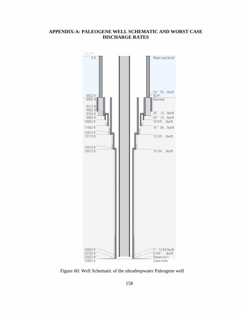
158
APPENDIX-A: PALEOGENE WELL SCHEMATIC AND WORST CASE
DISCHARGE RATES
Figure 60: Well Schematic of the ultradeepwater Paleogene well
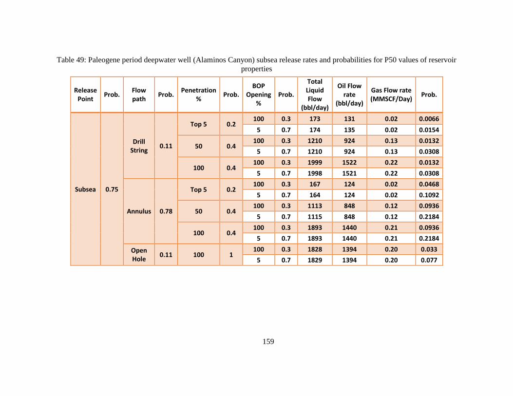
159
Table 49: Paleogene period deepwater well (Alaminos Canyon) subsea release rates and probabilities for P50 values of reservoir
properties
Release Point
Prob. Flow path
Prob. Penetration
% Prob.
BOP Opening
% Prob.
Total Liquid Flow
(bbl/day)
Oil Flow rate
(bbl/day)
Gas Flow rate (MMSCF/Day)
Prob.
Subsea 0.75
Drill String
0.11
Top 5 0.2 100 0.3 173 131 0.02 0.0066
5 0.7 174 135 0.02 0.0154
50 0.4 100 0.3 1210 924 0.13 0.0132
5 0.7 1210 924 0.13 0.0308
100 0.4 100 0.3 1999 1522 0.22 0.0132
5 0.7 1998 1521 0.22 0.0308
Annulus 0.78
Top 5 0.2 100 0.3 167 124 0.02 0.0468
5 0.7 164 124 0.02 0.1092
50 0.4 100 0.3 1113 848 0.12 0.0936
5 0.7 1115 848 0.12 0.2184
100 0.4 100 0.3 1893 1440 0.21 0.0936
5 0.7 1893 1440 0.21 0.2184
Open Hole
0.11 100 1 100 0.3 1828 1394 0.20 0.033
5 0.7 1829 1394 0.20 0.077
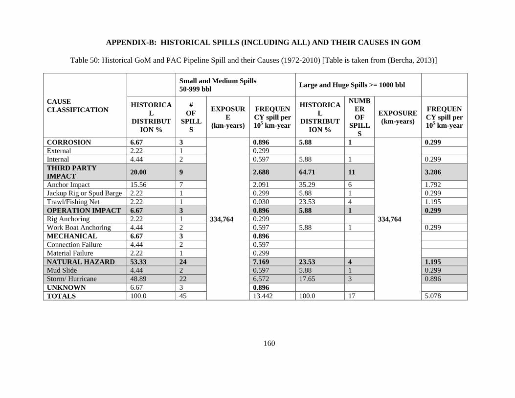
160
APPENDIX-B: HISTORICAL SPILLS (INCLUDING ALL) AND THEIR CAUSES IN GOM
Table 50: Historical GoM and PAC Pipeline Spill and their Causes (1972-2010) [Table is taken from (Bercha, 2013)]
CAUSE
CLASSIFICATION
Small and Medium Spills
50-999 bbl Large and Huge Spills >= 1000 bbl
HISTORICA
L
DISTRIBUT
ION %
#
OF
SPILL
S
EXPOSUR
E
(km-years)
FREQUEN
CY spill per
105 km-year
HISTORICA
L
DISTRIBUT
ION %
NUMB
ER
OF
SPILL
S
EXPOSURE
(km-years)
FREQUEN
CY spill per
105 km-year
CORROSION 6.67 3
334,764
0.896 5.88 1
334,764
0.299
External 2.22 1 0.299
Internal 4.44 2 0.597 5.88 1 0.299
THIRD PARTY
IMPACT 20.00 9 2.688 64.71 11 3.286
Anchor Impact 15.56 7 2.091 35.29 6 1.792
Jackup Rig or Spud Barge 2.22 1 0.299 5.88 1 0.299
Trawl/Fishing Net 2.22 1 0.030 23.53 4 1.195
OPERATION IMPACT 6.67 3 0.896 5.88 1 0.299
Rig Anchoring 2.22 1 0.299
Work Boat Anchoring 4.44 2 0.597 5.88 1 0.299
MECHANICAL 6.67 3 0.896
Connection Failure 4.44 2 0.597
Material Failure 2.22 1 0.299
NATURAL HAZARD 53.33 24 7.169 23.53 4 1.195
Mud Slide 4.44 2 0.597 5.88 1 0.299
Storm/ Hurricane 48.89 22 6.572 17.65 3 0.896
UNKNOWN 6.67 3 0.896
TOTALS 100.0 45 13.442 100.0 17 5.078
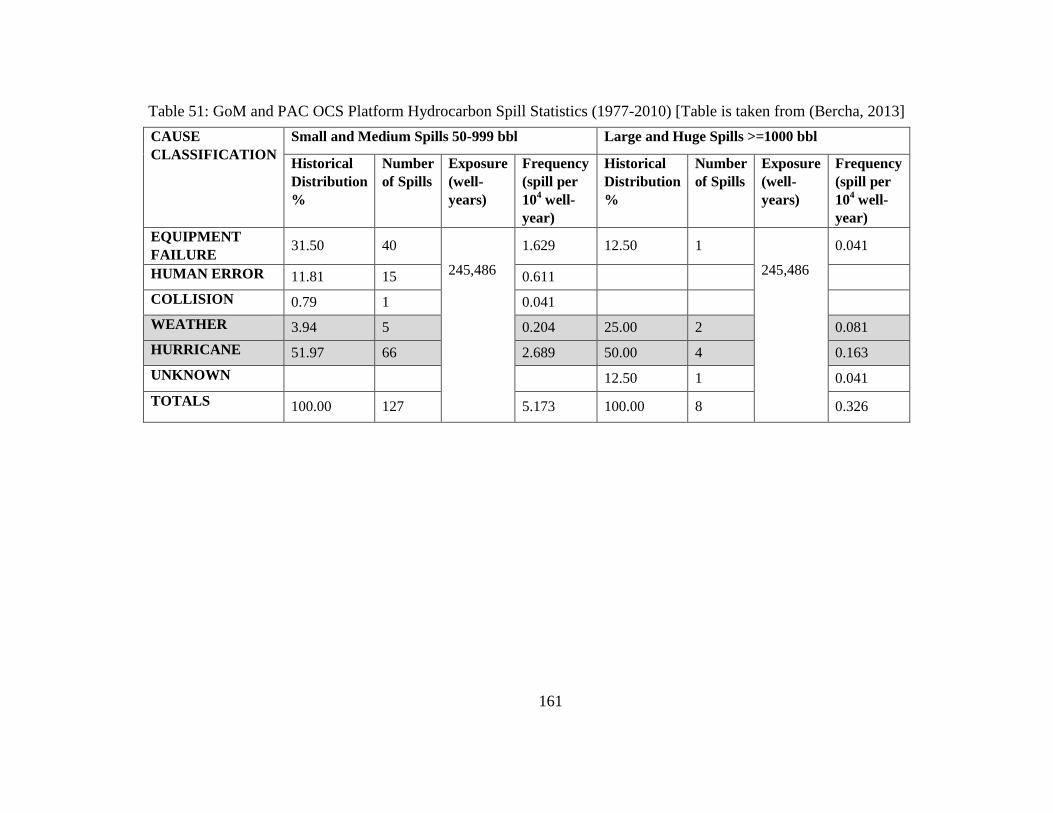
161
Table 51: GoM and PAC OCS Platform Hydrocarbon Spill Statistics (1977-2010) [Table is taken from (Bercha, 2013]
CAUSE
CLASSIFICATION
Small and Medium Spills 50-999 bbl Large and Huge Spills >=1000 bbl
Historical
Distribution
%
Number
of Spills
Exposure
(well-
years)
Frequency
(spill per
104 well-
year)
Historical
Distribution
%
Number
of Spills
Exposure
(well-
years)
Frequency
(spill per
104 well-
year)
EQUIPMENT
FAILURE 31.50 40
245,486
1.629 12.50 1
245,486
0.041
HUMAN ERROR 11.81 15 0.611
COLLISION 0.79 1 0.041
WEATHER 3.94 5 0.204 25.00 2 0.081
HURRICANE 51.97 66 2.689 50.00 4 0.163
UNKNOWN 12.50 1 0.041
TOTALS 100.00 127 5.173 100.00 8 0.326

162
VITA
Muhammad Zulqarnain was born in Sargodha, Pakistan. He completed his Master of
Science in Nuclear Engineering from Pakistan Institute of Engineering and Applied Science,
Islamabad, Pakistan, in 2003. After that he worked in a public sector organization in Pakistan for
four and half years. In August 2009, he joined The Craft and Hawkins Department of Petroleum
Engineering at Louisiana State University, Baton Rouge, Louisiana, for Master of Science. After
completing his Master of Science in Petroleum Engineering in May 2012, he continued for
Doctorate in Petroleum Engineering. The degree of Doctorate of Philosophy in Petroleum
Engineering will be conferred in August 2015.