Embed Size (px)
Citation preview

Deep Reinforcement Learning
via Policy Optimization
John Schulman
July 3, 2017

Introduction

Deep Reinforcement Learning: What to Learn?
I Policies (select next action)
I Value functions (measure goodness of states or state-action pairs)
I Models (predict next states and rewards)

Deep Reinforcement Learning: What to Learn?
I Policies (select next action)
I Value functions (measure goodness of states or state-action pairs)
I Models (predict next states and rewards)

Deep Reinforcement Learning: What to Learn?
I Policies (select next action)
I Value functions (measure goodness of states or state-action pairs)
I Models (predict next states and rewards)

Model Free RL: (Rough) Taxonomy
Policy Optimization Dynamic Programming
DFO / Evolution Policy Gradients Policy Iteration Value Iteration
Actor-Critic Methods
modified policy iteration
Q-Learning

Policy Optimization vs Dynamic Programming
I Conceptually . . .
I Policy optimization: optimize what you care aboutI Dynamic programming: indirect, exploit the problem structure,
self-consistency
I Empirically . . .
I Policy optimization more versatile, dynamic programming methods moresample-efficient when they work
I Policy optimization methods more compatible with rich architectures(including recurrence) which add tasks other than control (auxiliaryobjectives), dynamic programming methods more compatible withexploration and off-policy learning

Policy Optimization vs Dynamic Programming
I Conceptually . . .I Policy optimization: optimize what you care about
I Dynamic programming: indirect, exploit the problem structure,self-consistency
I Empirically . . .
I Policy optimization more versatile, dynamic programming methods moresample-efficient when they work
I Policy optimization methods more compatible with rich architectures(including recurrence) which add tasks other than control (auxiliaryobjectives), dynamic programming methods more compatible withexploration and off-policy learning

Policy Optimization vs Dynamic Programming
I Conceptually . . .I Policy optimization: optimize what you care aboutI Dynamic programming: indirect, exploit the problem structure,
self-consistency
I Empirically . . .
I Policy optimization more versatile, dynamic programming methods moresample-efficient when they work
I Policy optimization methods more compatible with rich architectures(including recurrence) which add tasks other than control (auxiliaryobjectives), dynamic programming methods more compatible withexploration and off-policy learning

Policy Optimization vs Dynamic Programming
I Conceptually . . .I Policy optimization: optimize what you care aboutI Dynamic programming: indirect, exploit the problem structure,
self-consistency
I Empirically . . .I Policy optimization more versatile, dynamic programming methods more
sample-efficient when they work
I Policy optimization methods more compatible with rich architectures(including recurrence) which add tasks other than control (auxiliaryobjectives), dynamic programming methods more compatible withexploration and off-policy learning

Policy Optimization vs Dynamic Programming
I Conceptually . . .I Policy optimization: optimize what you care aboutI Dynamic programming: indirect, exploit the problem structure,
self-consistency
I Empirically . . .I Policy optimization more versatile, dynamic programming methods more
sample-efficient when they workI Policy optimization methods more compatible with rich architectures
(including recurrence) which add tasks other than control (auxiliaryobjectives), dynamic programming methods more compatible withexploration and off-policy learning

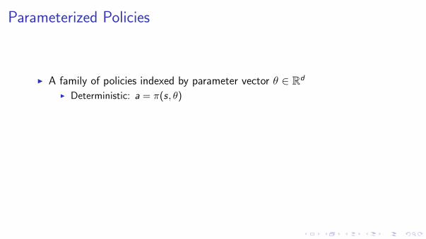
Parameterized Policies
I A family of policies indexed by parameter vector θ ∈ Rd
I Deterministic: a = π(s, θ)I Stochastic: π(a | s, θ)
I Analogous to classification or regression with input s, output a.
I Discrete action space: network outputs vector of probabilitiesI Continuous action space: network outputs mean and diagonal covariance of
Gaussian
Parameterized Policies
I A family of policies indexed by parameter vector θ ∈ Rd
I Deterministic: a = π(s, θ)
I Stochastic: π(a | s, θ)
I Analogous to classification or regression with input s, output a.
I Discrete action space: network outputs vector of probabilitiesI Continuous action space: network outputs mean and diagonal covariance of
Gaussian

Parameterized Policies
I A family of policies indexed by parameter vector θ ∈ Rd
I Deterministic: a = π(s, θ)I Stochastic: π(a | s, θ)
I Analogous to classification or regression with input s, output a.
I Discrete action space: network outputs vector of probabilitiesI Continuous action space: network outputs mean and diagonal covariance of
Gaussian

Parameterized Policies
I A family of policies indexed by parameter vector θ ∈ Rd
I Deterministic: a = π(s, θ)I Stochastic: π(a | s, θ)
I Analogous to classification or regression with input s, output a.I Discrete action space: network outputs vector of probabilities
I Continuous action space: network outputs mean and diagonal covariance ofGaussian
Parameterized Policies
I A family of policies indexed by parameter vector θ ∈ Rd
I Deterministic: a = π(s, θ)I Stochastic: π(a | s, θ)
I Analogous to classification or regression with input s, output a.I Discrete action space: network outputs vector of probabilitiesI Continuous action space: network outputs mean and diagonal covariance of
Gaussian

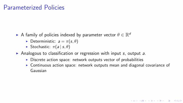
Episodic Setting
I In each episode, the initial state is sampled from µ, and the agent acts untilthe terminal state is reached. For example:
I Taxi robot reaches its destination (termination = good)I Waiter robot finishes a shift (fixed time)I Walking robot falls over (termination = bad)
I Goal: maximize expected return per episode
maximizeπ
E [R | π]
Episodic Setting
I In each episode, the initial state is sampled from µ, and the agent acts untilthe terminal state is reached. For example:
I Taxi robot reaches its destination (termination = good)
I Waiter robot finishes a shift (fixed time)I Walking robot falls over (termination = bad)
I Goal: maximize expected return per episode
maximizeπ
E [R | π]

Episodic Setting
I In each episode, the initial state is sampled from µ, and the agent acts untilthe terminal state is reached. For example:
I Taxi robot reaches its destination (termination = good)I Waiter robot finishes a shift (fixed time)
I Walking robot falls over (termination = bad)
I Goal: maximize expected return per episode
maximizeπ
E [R | π]

Episodic Setting
I In each episode, the initial state is sampled from µ, and the agent acts untilthe terminal state is reached. For example:
I Taxi robot reaches its destination (termination = good)I Waiter robot finishes a shift (fixed time)I Walking robot falls over (termination = bad)
I Goal: maximize expected return per episode
maximizeπ
E [R | π]

Derivative Free Optimization / Evolution

Cross Entropy Method
Initialize µ ∈ Rd , σ ∈ Rd
for iteration = 1, 2, . . . doCollect n samples of θi ∼ N(µ, diag(σ))Perform one episode with each θi , obtaining reward Ri
Select the top p% of θ samples (e.g. p = 20), the elite setFit a Gaussian distribution, to the elite set, updating µ, σ.
end forReturn the final µ.

Cross Entropy Method
I Sometimes works embarrassingly well
I. Szita and A. Lorincz. “Learning Tetris using the noisy
cross-entropy method”. Neural computation (2006)

Cross Entropy Method
I Sometimes works embarrassingly well
I. Szita and A. Lorincz. “Learning Tetris using the noisy
cross-entropy method”. Neural computation (2006)

Cross Entropy Method
I Sometimes works embarrassingly well
I. Szita and A. Lorincz. “Learning Tetris using the noisy
cross-entropy method”. Neural computation (2006)

Cross Entropy Method
I Sometimes works embarrassingly well
I. Szita and A. Lorincz. “Learning Tetris using the noisy
cross-entropy method”. Neural computation (2006)

Stochastic Gradient Ascent on Distribution
I Let µ define distribution for policy πθ: θ ∼ Pµ(θ)
I Return R depends on policy parameter θ and noise ζ
maximizeµ
Eθ,ζ [R(θ, ζ)]
R is unknown and possibly nondifferentiable
I “Score function” gradient estimator:
∇µEθ,ζ [R(θ, ζ)] = Eθ,ζ [∇µ logPµ(θ)R(θ, ζ)]
≈ 1
N
N∑i=1
∇µ logPµ(θi)Ri
Stochastic Gradient Ascent on Distribution
I Compare with cross-entropy method
I Score function grad:
∇µEθ,ζ [R(θ, ζ)] ≈ 1
N
N∑i=1
∇µ logPµ(θi )Ri
I Cross entropy method:
maximizeµ
1
N
N∑i=1
logPµ(θi )f (Ri ) (cross entropy method)
where f (r) = 1[r above threshold]

Stochastic Gradient Ascent on Distribution
I Compare with cross-entropy methodI Score function grad:
∇µEθ,ζ [R(θ, ζ)] ≈ 1
N
N∑i=1
∇µ logPµ(θi )Ri
I Cross entropy method:
maximizeµ
1
N
N∑i=1
logPµ(θi )f (Ri ) (cross entropy method)
where f (r) = 1[r above threshold]

Stochastic Gradient Ascent on Distribution
I Compare with cross-entropy methodI Score function grad:
∇µEθ,ζ [R(θ, ζ)] ≈ 1
N
N∑i=1
∇µ logPµ(θi )Ri
I Cross entropy method:
maximizeµ
1
N
N∑i=1
logPµ(θi )f (Ri ) (cross entropy method)
where f (r) = 1[r above threshold]

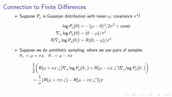
Connection to Finite DifferencesI Suppose Pµ is Gaussian distribution with mean µ, covariance σ2I
logPµ(θ) = −‖µ− θ‖2/2σ2 + const
∇µ logPµ(θ) = (θ − µ)/σ2
Ri∇µ logPµ(θi) = Ri(θi − µ)/σ2
I Suppose we do antithetic sampling, where we use pairs of samplesθ+ = µ + σz , θ− = µ− σz
1
2
(R(µ + σz , ζ)∇µ logPµ(θ+) + R(µ− σz , ζ ′)∇µ logPµ(θ−)
)=
1
σ
(R(µ + σz , ζ)− R(µ− σz , ζ ′)
)z
I Using same noise ζ for both evaluations reduces variance

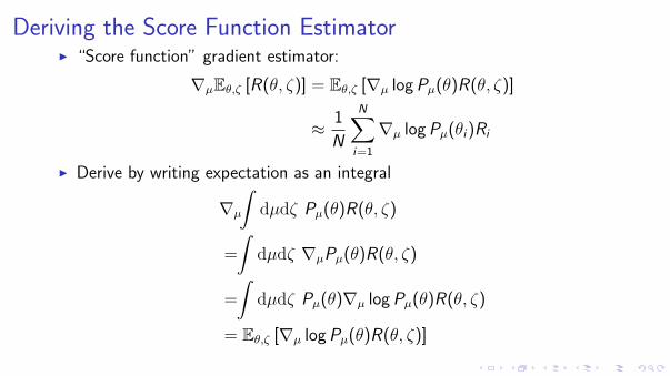
Deriving the Score Function EstimatorI “Score function” gradient estimator:
∇µEθ,ζ [R(θ, ζ)] = Eθ,ζ [∇µ logPµ(θ)R(θ, ζ)]
≈ 1
N
N∑i=1
∇µ logPµ(θi)Ri
I Derive by writing expectation as an integral
∇µ
∫dµdζ Pµ(θ)R(θ, ζ)
=
∫dµdζ ∇µPµ(θ)R(θ, ζ)
=
∫dµdζ Pµ(θ)∇µ logPµ(θ)R(θ, ζ)
= Eθ,ζ [∇µ logPµ(θ)R(θ, ζ)]
Deriving the Score Function EstimatorI “Score function” gradient estimator:
∇µEθ,ζ [R(θ, ζ)] = Eθ,ζ [∇µ logPµ(θ)R(θ, ζ)]
≈ 1
N
N∑i=1
∇µ logPµ(θi)Ri
I Derive by writing expectation as an integral
∇µ
∫dµdζ Pµ(θ)R(θ, ζ)
=
∫dµdζ ∇µPµ(θ)R(θ, ζ)
=
∫dµdζ Pµ(θ)∇µ logPµ(θ)R(θ, ζ)
= Eθ,ζ [∇µ logPµ(θ)R(θ, ζ)]

Literature on DFO
I Evolution strategies (Rechenberg and Eigen, 1973)
I Simultaneous perturbation stochastic approximation (Spall, 1992)
I Covariance matrix adaptation: popular relative of CEM (Hansen, 2006)
I Reward weighted regression (Peters and Schaal, 2007), PoWER (Kober andPeters, 2007)
Literature on DFO
I Evolution strategies (Rechenberg and Eigen, 1973)
I Simultaneous perturbation stochastic approximation (Spall, 1992)
I Covariance matrix adaptation: popular relative of CEM (Hansen, 2006)
I Reward weighted regression (Peters and Schaal, 2007), PoWER (Kober andPeters, 2007)

Literature on DFO
I Evolution strategies (Rechenberg and Eigen, 1973)
I Simultaneous perturbation stochastic approximation (Spall, 1992)
I Covariance matrix adaptation: popular relative of CEM (Hansen, 2006)
I Reward weighted regression (Peters and Schaal, 2007), PoWER (Kober andPeters, 2007)
Literature on DFO
I Evolution strategies (Rechenberg and Eigen, 1973)
I Simultaneous perturbation stochastic approximation (Spall, 1992)
I Covariance matrix adaptation: popular relative of CEM (Hansen, 2006)
I Reward weighted regression (Peters and Schaal, 2007), PoWER (Kober andPeters, 2007)
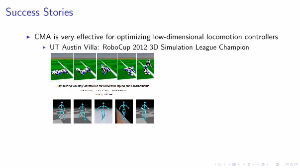
Success Stories
I CMA is very effective for optimizing low-dimensional locomotion controllers
I UT Austin Villa: RoboCup 2012 3D Simulation League Champion
I Evolution Strategies was shown to perform well on Atari, competetive withpolicy gradient methods (Salimans et al., 2017)
Success Stories
I CMA is very effective for optimizing low-dimensional locomotion controllersI UT Austin Villa: RoboCup 2012 3D Simulation League Champion
I Evolution Strategies was shown to perform well on Atari, competetive withpolicy gradient methods (Salimans et al., 2017)

Success Stories
I CMA is very effective for optimizing low-dimensional locomotion controllersI UT Austin Villa: RoboCup 2012 3D Simulation League Champion
I Evolution Strategies was shown to perform well on Atari, competetive withpolicy gradient methods (Salimans et al., 2017)

Policy Gradient Methods

Overview
Problem:
maximizeE [R | πθ]
I Here, we’ll use a fixed policy parameter θ (instead of sampling θ ∼ Pµ) andestimate gradient with respect to θ
I Noise is in action space rather than parameter space

Overview
Problem:
maximizeE [R | πθ]
I Here, we’ll use a fixed policy parameter θ (instead of sampling θ ∼ Pµ) andestimate gradient with respect to θ
I Noise is in action space rather than parameter space

Overview
Problem:
maximizeE [R | πθ]
Intuitions: collect a bunch of trajectories, and ...
1. Make the good trajectories more probable
2. Make the good actions more probable
3. Push the actions towards better actions

Overview
Problem:
maximizeE [R | πθ]
Intuitions: collect a bunch of trajectories, and ...
1. Make the good trajectories more probable
2. Make the good actions more probable
3. Push the actions towards better actions

Overview
Problem:
maximizeE [R | πθ]
Intuitions: collect a bunch of trajectories, and ...
1. Make the good trajectories more probable
2. Make the good actions more probable
3. Push the actions towards better actions

Score Function Gradient Estimator for PoliciesI Now random variable is a whole trajectoryτ = (s0, a0, r0, s1, a1, r1, . . . , sT−1, aT−1, rT−1, sT )
∇θEτ [R(τ)] = Eτ [∇θ logP(τ | θ)R(τ)]
I Just need to write out P(τ | θ):
P(τ | θ) = µ(s0)T−1∏t=0
[π(at | st , θ)P(st+1, rt | st , at)]
logP(τ | θ) = log µ(s0) +T−1∑t=0
[log π(at | st , θ) + logP(st+1, rt | st , at)]
∇θ logP(τ | θ) = ∇θ
T−1∑t=0
log π(at | st , θ)
∇θEτ [R] = Eτ
[R∇θ
T−1∑t=0
log π(at | st , θ)
]
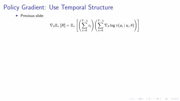
Policy Gradient: Use Temporal StructureI Previous slide:
∇θEτ [R] = Eτ
[(T−1∑t=0
rt
)(T−1∑t=0
∇θ log π(at | st , θ)
)]
I We can repeat the same argument to derive the gradient estimator for a single rewardterm rt′ .
∇θE [rt′ ] = E
rt′ t′∑t=0
∇θ log π(at | st , θ)
I Sum this formula over t, we obtain
∇θE [R] = E
T−1∑t=0
rt′t′∑t=0
∇θ log π(at | st , θ)
= E
[T−1∑t=0
∇θ log π(at | st , θ)T−1∑t′=t
rt′
]

Policy Gradient: Use Temporal StructureI Previous slide:
∇θEτ [R] = Eτ
[(T−1∑t=0
rt
)(T−1∑t=0
∇θ log π(at | st , θ)
)]I We can repeat the same argument to derive the gradient estimator for a single reward
term rt′ .
∇θE [rt′ ] = E
rt′ t′∑t=0
∇θ log π(at | st , θ)
I Sum this formula over t, we obtain
∇θE [R] = E
T−1∑t=0
rt′t′∑t=0
∇θ log π(at | st , θ)
= E
[T−1∑t=0
∇θ log π(at | st , θ)T−1∑t′=t
rt′
]
Policy Gradient: Introduce Baseline
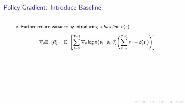
I Further reduce variance by introducing a baseline b(s)
∇θEτ [R] = Eτ
[T−1∑t=0
∇θ log π(at | st , θ)
(T−1∑t′=t
rt′ − b(st)
)]
I For any choice of b, gradient estimator is unbiased.
I Near optimal choice is expected return,b(st) ≈ E [rt + rt+1 + rt+2 + · · ·+ rT−1]
I Interpretation: increase logprob of action at proportionally to how muchreturns
∑T−1t=t′ rt′ are better than expected

Policy Gradient: Introduce Baseline
I Further reduce variance by introducing a baseline b(s)
∇θEτ [R] = Eτ
[T−1∑t=0
∇θ log π(at | st , θ)
(T−1∑t′=t
rt′ − b(st)
)]
I For any choice of b, gradient estimator is unbiased.
I Near optimal choice is expected return,b(st) ≈ E [rt + rt+1 + rt+2 + · · ·+ rT−1]
I Interpretation: increase logprob of action at proportionally to how muchreturns
∑T−1t=t′ rt′ are better than expected

Discounts for Variance Reduction
I Introduce discount factor γ, which ignores delayed effects between actionsand rewards
∇θEτ [R] ≈ Eτ
[T−1∑t=0
∇θ log π(at | st , θ)
(T−1∑t′=t
γt′−trt′ − b(st)
)]
I Now, we want b(st) ≈ E[rt + γrt+1 + γ2rt+2 + · · ·+ γT−1−trT−1
]I Write gradient estimator more generally as
∇θEτ [R] ≈ Eτ
[T−1∑t=0
∇θ log π(at | st , θ)At
]
At is the advantage estimate

Discounts for Variance Reduction
I Introduce discount factor γ, which ignores delayed effects between actionsand rewards
∇θEτ [R] ≈ Eτ
[T−1∑t=0
∇θ log π(at | st , θ)
(T−1∑t′=t
γt′−trt′ − b(st)
)]
I Now, we want b(st) ≈ E[rt + γrt+1 + γ2rt+2 + · · ·+ γT−1−trT−1
]
I Write gradient estimator more generally as
∇θEτ [R] ≈ Eτ
[T−1∑t=0
∇θ log π(at | st , θ)At
]
At is the advantage estimate

Discounts for Variance Reduction
I Introduce discount factor γ, which ignores delayed effects between actionsand rewards
∇θEτ [R] ≈ Eτ
[T−1∑t=0
∇θ log π(at | st , θ)
(T−1∑t′=t
γt′−trt′ − b(st)
)]
I Now, we want b(st) ≈ E[rt + γrt+1 + γ2rt+2 + · · ·+ γT−1−trT−1
]I Write gradient estimator more generally as
∇θEτ [R] ≈ Eτ
[T−1∑t=0
∇θ log π(at | st , θ)At
]
At is the advantage estimate

“Vanilla” Policy Gradient Algorithm
Initialize policy parameter θ, baseline bfor iteration=1, 2, . . . do
Collect a set of trajectories by executing the current policyAt each timestep in each trajectory, compute
the return Rt =∑T−1
t′=t γt′−trt′ , and
the advantage estimate At = Rt − b(st).Re-fit the baseline, by minimizing ‖b(st)− Rt‖2,
summed over all trajectories and timesteps.Update the policy, using a policy gradient estimate g ,
which is a sum of terms ∇θ log π(at | st , θ)At
end for

Advantage Actor-Critic
I Use neural network that represents policy πθ and value function Vθ(approximating V πθ)
I Pseudocode
for iteration=1, 2, . . . doAgent acts for T timesteps (e.g., T = 20),For each timestep t, compute
Rt = rt + γrt+1 + · · ·+ γT−t+1rT−1 + γT−tVθ(st)
At = Rt − Vθ(st)
Rt is target value function, in regression problemAt is estimated advantage function
Compute loss gradient g = ∇θ
∑Tt=1
[− log πθ(at | st)At + c(Vθ(s)− Rt)
2]
g is plugged into a stochastic gradient ascent algorithm, e.g., Adam.end for
V. Mnih, A. P. Badia, M. Mirza, A. Graves, T. P. Lillicrap, et al. “Asynchronous methods for deep reinforcement learning”. (2016)

Trust Region Policy Optimization
I Motivation: make policy gradients more robust and sample efficient
I Unlike in supervised learning, policy affects distribution of inputs, so a largebad update can be disastrous
I Makes use of a “surrogate objective” that estimates the performance of thepolicy around πold used for sampling
Lπold(π) =1
N
N∑i=1
π(ai | si)πold(ai | si)
Ai (1)
Differentiating this objective gives the policy gradient
I Lπold(π) is only accurate when state distribution of π is close to πold, thus itmakes sense to constrain or penalize the distance DKL [πold ‖ π]

Trust Region Policy Optimization
I Motivation: make policy gradients more robust and sample efficientI Unlike in supervised learning, policy affects distribution of inputs, so a large
bad update can be disastrous
I Makes use of a “surrogate objective” that estimates the performance of thepolicy around πold used for sampling
Lπold(π) =1
N
N∑i=1
π(ai | si)πold(ai | si)
Ai (1)
Differentiating this objective gives the policy gradient
I Lπold(π) is only accurate when state distribution of π is close to πold, thus itmakes sense to constrain or penalize the distance DKL [πold ‖ π]

Trust Region Policy OptimizationI Pseudocode:
for iteration=1, 2, . . . doRun policy for T timesteps or N trajectoriesEstimate advantage function at all timesteps
maximizeθ
N∑n=1
πθ(an | sn)
πθold(an | sn)An
subject to KLπθold (πθ) ≤ δ
end for
I Can solve constrained optimization problem efficiently by using conjugategradient
I Closely related to natural policy gradients (Kakade, 2002), natural actorcritic (Peters and Schaal, 2005), REPS (Peters et al., 2010)

“Proximal” Policy Optimization
I Use penalty instead of constraint
maximizeθ
N∑n=1
πθ(an | sn)
πθold(an | sn)An − C ·KLπθold (πθ)
I Pseudocode:
for iteration=1, 2, . . . doRun policy for T timesteps or N trajectoriesEstimate advantage function at all timestepsDo SGD on above objective for some number of epochsIf KL too high, increase β. If KL too low, decrease β.
end for
I ≈ same performance as TRPO, but only first-order optimization

Variance Reduction for Policy Gradients

Reward Shaping

Reward Shaping
I Reward shaping: δ(s, a, s ′) = r(s, a, s ′) + γΦ(s ′)− Φ(s) for arbitrary“potential” Φ
I Theorem: δ admits the same optimal policies as r .1
I Proof sketch: suppose Q∗ satisfies Bellman equation (T Q = Q). If wetransform r → δ, policy’s value function satisfies Q(s, a) = Q∗(s, a)− Φ(s)
I Q∗ satisfies Bellman equation ⇒ Q also satisfies Bellman equation
1A. Y. Ng, D. Harada, and S. Russell. “Policy invariance under reward transformations: Theory and application to reward shaping”. ICML. 1999.

Reward ShapingI Theorem: δ admits the same optimal policies as R. A. Y. Ng, D. Harada, and S. Russell.
“Policy invariance under reward transformations: Theory and application to rewardshaping”. ICML. 1999
I Alternative proof: advantage function is invariant. Let’s look at effect on V π and Qπ:
E[δ0 + γδ1 + γ2δ2 + . . .
]= E
[(r0 + γΦ(s1)− Φ(s0)) + γ(r1 + γΦ(s2)− Φ(s1)) + γ2(r2 + γΦ(s3)− Φ(s2)) + . . .
]= E
[r0 + γr1 + γ2r2 + · · · − Φ(s0)
]Thus,
V π(s) = V π(s)− Φ(s)
Qπ(s) = Qπ(s, a)− Φ(s)
Aπ(s) = Aπ(s, a)
Aπ(s, π(s)) = 0 at all states ⇒ π is optimal

Reward Shaping and Problem Difficulty
I Shape with Φ = V ∗ ⇒ problem is solved in one step of value iteration
I Shaping leaves policy gradient invariant (and just adds baseline to estimator)
E[∇θ log πθ(a0 | s0)(r0 + γΦ(s1)− Φ(s0)) + γ(r1 + γΦ(s2)− Φ(s1))
+ γ2(r2 + γΦ(s3)− Φ(s2)) + . . .]
= E[∇θ log πθ(a0 | s0)(r0 + γr1 + γ2r2 + · · · − Φ(s0))
]= E
[∇θ log πθ(a0 | s0)(r0 + γr1 + γ2r2 + . . . )
]

Reward Shaping and Policy Gradients
I First note connection between shaped reward and advantage function:
Es1 [r0 + γV π(s1)− V π(s0) | s0 = s, a0 = a] = Aπ(s, a)
Now considering the policy gradient and ignoring all but first shaped reward (i.e., pretendγ = 0 after shaping) we get
E
[∑t
∇θ log πθ(at | st)δt
]= E
[∑t
∇θ log πθ(at | st)(rt + γV π(st+1)− V π(st))
]
= E
[∑t
∇θ log πθ(at | st)Aπ(st , at)
]
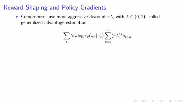
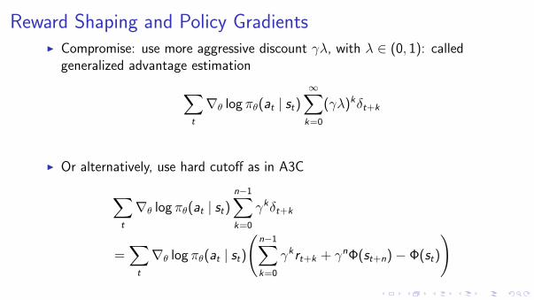
Reward Shaping and Policy GradientsI Compromise: use more aggressive discount γλ, with λ ∈ (0, 1): called
generalized advantage estimation∑t
∇θ log πθ(at | st)∞∑k=0
(γλ)kδt+k
I Or alternatively, use hard cutoff as in A3C
∑t
∇θ log πθ(at | st)n−1∑k=0
γkδt+k
=∑t
∇θ log πθ(at | st)
(n−1∑k=0
γkrt+k + γnΦ(st+n)− Φ(st)
)

Reward Shaping—Summary
I Reward shaping transformation leaves policy gradient and optimal policyinvariant
I Shaping with Φ ≈ V π makes consequences of actions more immediate
I Shaping, and then ignoring all but first term, gives policy gradient
Reward Shaping—Summary
I Reward shaping transformation leaves policy gradient and optimal policyinvariant
I Shaping with Φ ≈ V π makes consequences of actions more immediate
I Shaping, and then ignoring all but first term, gives policy gradient
Reward Shaping—Summary
I Reward shaping transformation leaves policy gradient and optimal policyinvariant
I Shaping with Φ ≈ V π makes consequences of actions more immediate
I Shaping, and then ignoring all but first term, gives policy gradient

Aside: Reward Shaping is Crucial in PracticeI I. Mordatch, E. Todorov, and Z. Popovic. “Discovery of complex behaviors through
contact-invariant optimization”. ACM Transactions on Graphics (TOG) 31.4 (2012),p. 43
I Y. Tassa, T. Erez, and E. Todorov. “Synthesis and stabilization of complex behaviorsthrough online trajectory optimization”. Intelligent Robots and Systems (IROS), 2012IEEE/RSJ International Conference on. IEEE. 2012, pp. 4906–4913
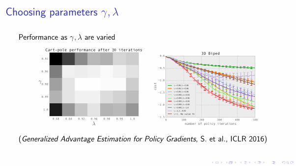
Choosing parameters γ, λ
Performance as γ, λ are varied
0 100 200 300 400 500
number of policy iterations
2.5
2.0
1.5
1.0
0.5
0.0
cost
3D Biped
γ=0.96,λ=0.96
γ=0.98,λ=0.96
γ=0.99,λ=0.96
γ=0.995,λ=0.92
γ=0.995,λ=0.96
γ=0.995,λ=0.98
γ=0.995,λ=0.99
γ=0.995,λ=1.0
γ=1,λ=0.96
γ=1, No value fn
(Generalized Advantage Estimation for Policy Gradients, S. et al., ICLR 2016)

Pathwise Derivative Methods
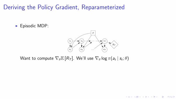
Deriving the Policy Gradient, Reparameterized
I Episodic MDP:
θ
s1 s2 . . . sT
a1 a2 . . . aT
RT
Want to compute ∇θE [RT ]. We’ll use ∇θ log π(at | st ; θ)
I Reparameterize: at = π(st , zt ; θ). zt is noise from fixed distribution.
I Only works if P(s2 | s1, a1) is known _

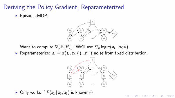
Deriving the Policy Gradient, ReparameterizedI Episodic MDP:
θ
s1 s2 . . . sT
a1 a2 . . . aT
RT
Want to compute ∇θE [RT ]. We’ll use ∇θ log π(at | st ; θ)I Reparameterize: at = π(st , zt ; θ). zt is noise from fixed distribution.
θ
s1 s2 . . . sT
a1 a2 . . . aT
z1 z2 . . . zT
RT
I Only works if P(s2 | s1, a1) is known _

Using a Q-function
θ
s1 s2 . . . sT
a1 a2 . . . aT
z1 z2 . . . zT
RT
d
dθE [RT ] = E
[T∑t=1
dRT
dat
datdθ
]= E
[T∑t=1
d
datE [RT | at ]
datdθ
]
= E
[T∑t=1
dQ(st , at)
dat
datdθ
]= E
[T∑t=1
d
dθQ(st , π(st , zt ; θ))
]

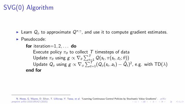
SVG(0) Algorithm
I Learn Qφ to approximate Qπ,γ, and use it to compute gradient estimates.
I Pseudocode:
for iteration=1, 2, . . . doExecute policy πθ to collect T timesteps of dataUpdate πθ using g ∝ ∇θ
∑Tt=1Q(st , π(st , zt ; θ))
Update Qφ using g ∝ ∇φ
∑Tt=1(Qφ(st , at)− Qt)
2, e.g. with TD(λ)end for
N. Heess, G. Wayne, D. Silver, T. Lillicrap, Y. Tassa, et al. “Learning Continuous Control Policies by Stochastic Value Gradients”. arXivpreprint arXiv:1510.09142 (2015)

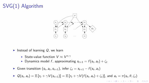
SVG(1) Algorithm
θ
s1 s2 . . . sT
a1 a2 . . . aT
z1 z2 . . . zT
RT
I Instead of learning Q, we learn
I State-value function V ≈ V π,γ
I Dynamics model f , approximating st+1 = f (st , at) + ζt
I Given transition (st , at , st+1), infer ζt = st+1 − f (st , at)
I Q(st , at) = E [rt + γV (st+1)] = E [rt + γV (f (st , at) + ζt)], and at = π(st , θ, ζt)

SVG(∞) Algorithm
θ
s1 s2 . . . sT
a1 a2 . . . aT
z1 z2 . . . zT
RT
I Just learn dynamics model f
I Given whole trajectory, infer all noise variables
I Freeze all policy and dynamics noise, differentiate through entire deterministiccomputation graph

SVG(∞) Algorithm
θ
s1 s2 . . . sT
a1 a2 . . . aT
z1 z2 . . . zT
RT
I Just learn dynamics model f
I Given whole trajectory, infer all noise variables
I Freeze all policy and dynamics noise, differentiate through entire deterministiccomputation graph

SVG(∞) Algorithm
θ
s1 s2 . . . sT
a1 a2 . . . aT
z1 z2 . . . zT
RT
I Just learn dynamics model f
I Given whole trajectory, infer all noise variables
I Freeze all policy and dynamics noise, differentiate through entire deterministiccomputation graph

SVG Results
I Applied to 2D robotics tasks
I Overall: different gradient estimators behave similarly
N. Heess, G. Wayne, D. Silver, T. Lillicrap, Y. Tassa, et al. “Learning Continuous Control Policies by Stochastic Value Gradients”. arXivpreprint arXiv:1510.09142 (2015)

SVG Results
I Applied to 2D robotics tasks
I Overall: different gradient estimators behave similarly
N. Heess, G. Wayne, D. Silver, T. Lillicrap, Y. Tassa, et al. “Learning Continuous Control Policies by Stochastic Value Gradients”. arXivpreprint arXiv:1510.09142 (2015)

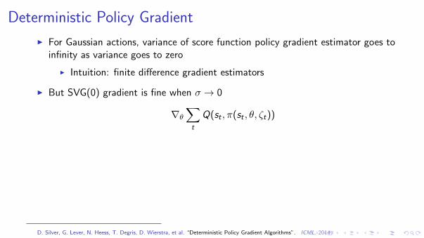
Deterministic Policy Gradient
I For Gaussian actions, variance of score function policy gradient estimator goes toinfinity as variance goes to zero
I Intuition: finite difference gradient estimators
I But SVG(0) gradient is fine when σ → 0
∇θ∑t
Q(st , π(st , θ, ζt))
I Problem: there’s no exploration.
I Solution: add noise to the policy, but estimate Q with TD(0), so it’s validoff-policy
I Policy gradient is a little biased (even with Q = Qπ), but only because statedistribution is off—it gets the right gradient at every state
D. Silver, G. Lever, N. Heess, T. Degris, D. Wierstra, et al. “Deterministic Policy Gradient Algorithms”. ICML. 2014

Deep Deterministic Policy GradientI Incorporate replay buffer and target network ideas from DQN for increased
stability
I Use lagged (Polyak-averaging) version of Qφ and πθ for fitting Qφ (towardsQπ,γ) with TD(0)
Qt = rt + γQφ′(st+1, π(st+1; θ′))
I Pseudocode:
for iteration=1, 2, . . . doAct for several timesteps, add data to replay bufferSample minibatchUpdate πθ using g ∝ ∇θ
∑Tt=1 Q(st , π(st , zt ; θ))
Update Qφ using g ∝ ∇φ
∑Tt=1(Qφ(st , at)− Qt)
2,end for
T. P. Lillicrap, J. J. Hunt, A. Pritzel, N. Heess, T. Erez, et al. “Continuous control with deep reinforcement learning”. arXiv preprintarXiv:1509.02971 (2015)

DDPG Results
Applied to 2D and 3D robotics tasks and driving with pixel input
T. P. Lillicrap, J. J. Hunt, A. Pritzel, N. Heess, T. Erez, et al. “Continuous control with deep reinforcement learning”. arXiv preprintarXiv:1509.02971 (2015)
Policy Gradient Methods: Comparison
I Two kinds of policy gradient estimator
I REINFORCE / score function estimator: ∇ log π(a | s)A.
I Learn Q or V for variance reduction, to estimate A
I Pathwise derivative estimators (differentiate wrt action)
I SVG(0) / DPG: ddaQ(s, a) (learn Q)
I SVG(1): dda (r + γV (s ′)) (learn f ,V )
I SVG(∞): ddat
(rt + γrt+1 + γ2rt+2 + . . . ) (learn f )
I Pathwise derivative methods more sample-efficient when they work (maybe),but work less generally due to high bias

Policy Gradient Methods: Comparison
I Two kinds of policy gradient estimatorI REINFORCE / score function estimator: ∇ log π(a | s)A.
I Learn Q or V for variance reduction, to estimate AI Pathwise derivative estimators (differentiate wrt action)
I SVG(0) / DPG: ddaQ(s, a) (learn Q)
I SVG(1): dda (r + γV (s ′)) (learn f ,V )
I SVG(∞): ddat
(rt + γrt+1 + γ2rt+2 + . . . ) (learn f )
I Pathwise derivative methods more sample-efficient when they work (maybe),but work less generally due to high bias

Policy Gradient Methods: Comparison
I Two kinds of policy gradient estimatorI REINFORCE / score function estimator: ∇ log π(a | s)A.
I Learn Q or V for variance reduction, to estimate AI Pathwise derivative estimators (differentiate wrt action)
I SVG(0) / DPG: ddaQ(s, a) (learn Q)
I SVG(1): dda (r + γV (s ′)) (learn f ,V )
I SVG(∞): ddat
(rt + γrt+1 + γ2rt+2 + . . . ) (learn f )
I Pathwise derivative methods more sample-efficient when they work (maybe),but work less generally due to high bias

Thanks
Questions?


![Automated Deep Reinforcement Learning Environment for ... · Trust Region Policy Optimization (TRPO) [9] and Deep Deterministic Policy Gradient (DDPG) [10] directly on the. hardware](https://img.pdfslide.us/doc/110x75/5f62089485e8ca7d785a16d7/automated-deep-reinforcement-learning-environment-for-trust-region-policy-optimization.jpg)


![Deep Reinforcement Learning in System Optimization · arXiv:1908.01275v2 [cs.LG] 7 Aug 2019. Deep Reinforcement Learning in System Optimization Figure 1. Reinforcement learning. By](https://img.pdfslide.us/doc/110x75/5f14fb8d1a5cf26de94ee32f/deep-reinforcement-learning-in-system-optimization-arxiv190801275v2-cslg-7.jpg)