1

Deep Recurrent Regression for Facial LandmarkDetection

Hanjiang Lai, Shentao Xiao, Yan Pan, Zhen Cui, Jiashi Feng, Chunyan Xu, Jian Yin, Shuicheng Yan, SeniorMember, IEEE

Abstract—We propose a novel end-to-end deep architecturefor face landmark detection, based on a deep convolutional anddeconvolutional network followed by carefully designed recurrentnetwork structures. The pipeline of this architecture consists ofthree parts. Through the first part, we encode an input face imageto resolution-preserved deconvolutional feature maps via a deepnetwork with stacked convolutional and deconvolutional layers.Then, in the second part, we estimate the initial coordinates ofthe facial key points by an additional convolutional layer on topof these deconvolutional feature maps. In the last part, by usingthe deconvolutional feature maps and the initial facial key pointsas input, we refine the coordinates of the facial key points bya recurrent network that consists of multiple Long-Short TermMemory (LSTM) components. Extensive evaluations on severalbenchmark datasets show that the proposed deep architecturehas superior performance against the state-of-the-art methods.

Index Terms—Cascaded Regression, Facial Landmark Detec-tion, Shape-indexed Features, Recurrent Regression.

I. INTRODUCTION

Facial landmark detection is a task of automatically locatingpre-defined facial key points on a human face. It is one of thecore techniques for solving various facial analysis problems,e.g., face recognition [1], face morphing [2], [3], 3D facemodeling [4] and face beautification [2]. In recent years,considerable research effort has been devoted to developingmodels for accurately localizing the landmark points on theface images captured under unconstrained conditions basedon the provided face detection bounding box [5]–[7]. Amongthese methods, a notable research line is the cascaded regres-sion methods [8]–[11], which have shown a strong ability toefficiently and accurately localize the facial key points evenin challenging scenarios.

The cascaded regression methods are characterized by sucha pipeline: at each cascading stage, visual features are firstextracted from the current predicted landmark points; the coor-dinates of the landmark points are then updated via regressionfrom the extracted features; and the updated landmark pointsare used for regression in the next stage. These operations arerepeated for several times to iteratively refine the predictedlocations of landmark points.

Hanjiang Lai, Yan Pan and Jian Yin are with School of Data and ComputerScience, Sun Yat-Sen University, China. This work was mainly performedwhen Hanjiang Lai was staying in NUS.

Shengtao Xiao, Zhen Cui Jiashi Feng and Shuicheng Yan are with De-partment of Electronic and Computer Engineering, National University ofSingapore, Singapore.

Chunyan Xu is with School of Computer Science and Engineering, NanjingUniversity of Science and Technology, China.

Hanjiang Lai and Shengtao Xiao contributed equally to this work. Yan Panis the Corresponding Author (panyan@mail.sysu.edu.cn).

Despite of their acknowledged success, the performanceof such cascaded regression methods heavily depends on thequality of the adopted visual features. Most of the existingcascaded regression methods employ popular hand-crafted fea-tures such as SIFT, HOG [9], [12] or binary features extractedby random forest models [13]. However, such hand-craftedfeatures may not be optimally compatible with the processof cascaded regression, making the learned models usually besensitive to large occlusion, extreme poses of human faces,large facial expressions, or varying illumination conditions.

In addition, in the k-th cascading stage of the existingcascaded regression methods (e.g., SDM [9]), only the currentestimated coordinates of landmarks (denoted as Sk) are usedto conduct regression, but ignoring the landmark informationestimated in more previous iterations (i.e., S0, S1, ..., Sk−1).Since the cascaded regression iteratively refines a set ofestimated landmarks, these estimated sets of landmarks (i.e.,S0, S1, ..., Sk−1, Sk) are expected to have high correlation toeach other. We argue that, in the k-th cascading stage, if wecould effectively incorporate all of S0, S1, ..., Sk−1, Sk intolearning, we would improve the performance of regression.

In this paper, we propose a deep end-to-end architecturethat iteratively refines the estimated coordinates of the faciallandmark points. This deep architecture can be regarded as a“mimicry” of the cascaded regression based on deep networks.The key insight of the proposed architecture is to combine thestrength of convolutional neural networks (CNNs) for learningbetter feature representation and recurrent neural networks(RNNs) for memorizing the previous estimated information oflandmark points. Specially, as shown in Fig. 1, this architecturehas three building blocks: (1) an input face image is firstlyencoded to resolution-preserved deconvolutional feature maps,each is in the same size of the input image, via stacked convo-lutional and deconvolutional layers. (2) On top of these decon-volutional feature maps, we construct a small sub-network toestimate the initial coordinates of the facial landmark pointsby adding an additional convolutional layer. Such estimatedinitial facial landmarks provide a good starting point for thefurther refinement of the estimated landmarks. (3) With thedeconvolutional feature maps and the initial facial landmarks,we construct a carefully designed recurrent network withmultiple Long-Short Term Memory (LSTM) components toiteratively refine the estimated coordinates of the facial keypoints. This recurrent network can be regarded as a “mimicry”of the pipeline of cascaded regression methods. For eachLSTM component, visual features are directly extracted fromthe deconvolutional feature maps via the proposed shape-

arX

iv:1

510.

0908

3v3

[cs

.CV

] 3

1 O

ct 2

016

2

(A) Spatial Resolution-Preserved Conv-Deconv Network

256

256

conv5conv1 conv2 deconv6 deconv7

96

256

256

96

128

128

(B) Initialization Network

SIP

+

64

64128

128256

256

……

…

(C) Deep Recurrent Regression

LSTM

+…

…

+

SIP

LSTM

+…

…

SIP

LSTM

+…

…

+

Memory Cell:

Regression Regression Regression

…

68

256

256

Initialization…

conv8

(D) Shape-Indexed Pooling (SIP)

deconv7

Max Pooling

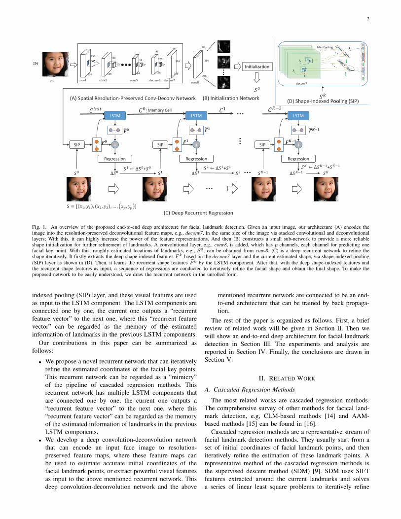
Fig. 1. An overview of the proposed end-to-end deep architecture for facial landmark detection. Given an input image, our architecture (A) encodes theimage into the resolution-preserved deconvolutional feature maps, e.g., deconv7, in the same size of the image via stacked convolutional and deconvolutionallayers; With this, it can highly increase the power of the feature representations. And then (B) constructs a small sub-network to provide a more reliableshape initialization for further refinement of landmarks. A convolutional layer, e.g., conv8, is added, which has p channels, each channel for predicting onefacial key point. With this, roughly estimated locations of landmarks, e.g., S0, can be obtained from conv8. (C) is a deep recurrent network to refine theshape iteratively. It firstly extracts the deep shape-indexed features Fk based on the deconv7 layer and the current estimated shape, via shape-indexed pooling(SIP) layer as shown in (D). Then, it learns the recurrent shape features Fk by the LSTM component. After that, with the deep shape-indexed features andthe recurrent shape features as input, a sequence of regressions are conducted to iteratively refine the facial shape and obtain the final shape. To make theproposed network to be easily understood, we draw the recurrent network in the unrolled form.

indexed pooling (SIP) layer, and these visual features are usedas input to the LSTM component. The LSTM components areconnected one by one, the current one outputs a “recurrentfeature vector” to the next one, where this “recurrent featurevector” can be regarded as the memory of the estimatedinformation of landmarks in the previous LSTM components.

Our contributions in this paper can be summarized asfollows:

• We propose a novel recurrent network that can iterativelyrefine the estimated coordinates of the facial key points.This recurrent network can be regarded as a “mimicry”of the pipeline of cascaded regression methods. Thisrecurrent network has multiple LSTM components thatare connected one by one, the current one outputs a“recurrent feature vector” to the next one, where this“recurrent feature vector” can be regarded as the memoryof the estimated information of landmarks in the previousLSTM components.

• We develop a deep convolution-deconvolution networkthat can encode an input face image to resolution-preserved feature maps, where these feature maps canbe used to estimate accurate initial coordinates of thefacial landmark points, or extract powerful visual featuresas input to the above mentioned recurrent network. Thisdeep convolution-deconvolution network and the above

mentioned recurrent network are connected to be an end-to-end architecture that can be trained by back propaga-tion.

The rest of the paper is organized as follows. First, a briefreview of related work will be given in Section II. Then wewill show an end-to-end deep architecture for facial landmarkdetection in Section III. The experiments and analysis arereported in Section IV. Finally, the conclusions are drawn inSection V.

II. RELATED WORK

A. Cascaded Regression Methods

The most related works are cascaded regression methods.The comprehensive survey of other methods for facical land-mark detection, e.g, CLM-based methods [14] and AAM-based methods [15] can be found in [16].

Cascaded regression methods are a representative stream offacial landmark detection methods. They usually start from aset of initial coordinates of facial landmark points, and theniteratively refine the estimation of these landmark points. Arepresentative method of the cascaded regression methods isthe supervised descent method (SDM) [9]. SDM uses SIFTfeatures extracted around the current landmarks and solvesa series of linear least square problems to iteratively refine

3

these landmarks. Ren et al. [13] propose the locality principleto learn a set of local binary features for cascade regression.Global SDM (GSDM) [17] is an extension to SDM whichdivides the search space into regions of similar gradientdirections.

In the last few years, we are witnessing dramatic progressin deep convolutional networks. In contrast to the methodsthat use hand-crafted visual features (e.g, SIFT, LBP), deep-convolutional-networks-based methods can automatically learndiscriminative visual features from images. Sun et al. [18]propose an approach to predict facial key points with three-level convolutional networks. Liu et al. [19] propose a dualsparse constrained cascaded regression model for robust faciallandmark detection. Zhang et al. [20] propose a Coarse-to-FineAuto-encoder Networks (CFAN) for facial alignment. Zhang etal. [21] propose a topic-aware face alignment method to dividethe difficult task of estimating the target landmarks into severalmuch easier subtasks. DRN-SSR [22] is a deep regressionnetwork coupled with sparse shape regression to predict theunion of all types of landmarks by leveraging datasets withvarying annotations. Belharbi et al. [23] formulate the facealignment as a structured output problem and exploit the strongdependencies between the outputs.

The performance of cascaded regression methods may heav-ily depend on the quality of initial face landmarks in the testingstage. Several methods have been developed to obtain a goodinitialization of face landmarks, including multiple randomshape initializations [8], smart restarts [24] and coarse-to-finesearching [12], [18], [20]. Cao et al. [8] run the cascadedregression method several times, each with a different initialshape, and take the median results as the final landmarkestimation. Zhu et al. [12] propose a coarse-to-fine searchingmethod that begins with a coarse search over a shape spacewith diverse shapes, and employs the coarse solution toconstrain subsequent finer search of shapes. Zhang et al. [20]propose a coarse-to-fine auto-encoder network to find theinitial shapes.

Different from the conventional cascaded regression ap-proach, in this paper, we propose a novel recurrent networkthat can iteratively refine the estimated facial landmarks, wherethis recurrent network can be regarded as a “mimicry” of thepipeline of cascaded regression methods.

We develop a carefully-designed deep convolution-deconvolution network that encodes an input face image toresolution-preserved deconvolutional feature maps. The visualfeatures for facial landmark detection are directly extractedfrom these feature maps. This shares some similarities to thedeep-convolutional-networks-based methods (e.g., [18]–[20])but we use a quite different deep architecture.

Different from the existing initialization strategies for facialshapes in the testing stage, by adding a simple sub-networkon top of the deconvolutional feature maps, we obtain initialface shapes from the output of this sub-network.

B. Recurrent Neural NetworksRecently, Recurrent Neural Networks (RNNs) have received

a lot of attention and achieved impressive results in vari-ous applications, including speech recognition [25], image

captioning [26] and video description [27]. RNNs have alsobeen applied to facial landmark detection. Very recently, Penget al. [28] propose a recurrent encoder-decoder network forvideo-based sequential facial landmark detection. They userecurrent networks to align a sequence of the same face invideo frames, by exploiting recurrent learning in spatial andtemporal dimensions.

Different to the method in [28] for video-based sequentialfacial landmark detection, in this paper, we focus on faciallandmark detection in still images and use recurrent networksto iteratively refine the estimated facial landmarks.

In addition, the proposed recurrent network in this papercontains multiple Long-Short Term Memory (LSTM) compo-nents. For self-containness, we give a brief introduction toLSTM. LSTM is one type of the RNNs, which is attractivebecause it is explicitly designed to remember information forlong periods of time. LSTM takes xt, ht−1 and ct−1 as inputs,ht and ct as outputs:

it = σ(Wi[xt;ht−1] + bi)

ft = σ(Wf [xt;ht−1] + bf )

ot = σ(Wo[xt;ht−1] + bo)

gt = tanh(Wg[xt;ht−1] + bg)

ct = ft � ct−1 + it � gtht = ot � ct,

where σ(x) = (1 + e−x)−1 is the sigmoid function. Theoutputs of the sigmoid functions are in the range of [0, 1],here the smaller values indicate “more probability to forgetthe previous information” and the larger values indicate “moreprobability to remember the information”. tanh(x) = ex−e−x

ex+e−x

is the tangent non-linearity function and its outputs are in therange [−1, 1]. [x;h] represents the concatenation of x and h.LSTM has four gates, a forget gate ft, an input gate it, anoutput gate ot and an input modulation gate gt. ht and ct arethe outputs. ht is the hidden unit. ct is the memory cell thatcan be learned to control whether the previous informationshould be forgotten or remembered.

III. THE APPROACH

The objective function of the traditional cascaded regressionmethods [9] can be formulated as

min∆Sk||φ(Sk + ∆Sk)− φ(S∗)||22, k = 0, · · · ,K − 1, (1)

where S is in the form of S = {(x1, y1), (x2, y2), ..., (xp, yp)}that (xi, yi) represents the coordinate of the i-th facial keypoint (i = 1, 2, ..., p). S∗ is the ground truth and S0 is the ini-tial configuration of the landmarks (e.g., the mean shape of alltraining images). We denote φ(S) as the shape-indexed featureextracted from the shape S. ∆S is the shape increment, whichis needed to be learned. The goal of cascaded regression is togenerate a sequence of updates (∆S0, . . . ,∆SK−1) startingfrom S0 and converges to S∗ (i.e., S0 +

∑K−1k=0 ∆Sk ≈ S∗).

For the traditional cascaded regression method, only thecurrent shape Sk is considered in the k-th regression, little in-formation about the previous shapes (e.g., S0, S1, · · · , Sk−1)

4

is kept. We argue that the cascade regression should be ableto connect previous shape information to the present shaperegression. We introduce a new feature F k 1 into (1). Theobjective function is changed to

min∆Sk||φ(Sk + ∆Sk) + F k − φ(S∗)||22. (2)

The new feature is referred as recurrent shape feature,which is used to incorporate the previous information and helpto improve the current prediction. Due to LSTMs have thestrong ability of learning long-term dependencies, we utilizethe LSTM to learn the recurrent shape feature (please referSubSection III-C for more details).

Let F k = φ(Sk) and f(Sk + ∆Sk) = ||φ(Sk + ∆Sk) +F k −φ(S∗)||22. Similar to SDM [9], we also assume that φ istwice differentiable under a small shape change. The Taylorexpansion of f(Sk + ∆Sk) is

f(Sk+∆Sk) ≈ f(Sk)+f′(Sk)T∆Sk+

1

2(∆Sk)T f

′′(Sk)∆Sk,

(3)where f

′′(Sk) and f

′(Sk) are the Hessian and Jacobian

matrices of f at Sk. Now the optimization objective becomes

min∆Sk

f(Sk) + f′(Sk)T∆Sk +

1

2(∆Sk)T f

′′(Sk)∆Sk, (4)

where ∆Sk is the variable. By letting the derivatives of theobjective in (4) with respect to ∆Sk to be zeros, we have

∆Sk = −[f′′(Sk)]−1f

′(Sk). (5)

According to the chain rule, we have f′(Sk) = ∂f

∂Sk =∂f∂φ ×

∂φ∂Sk = 2× (φ(Sk)+ F k−φ(S∗))×φ′(Sk). Substituting

it into (5), we have

∆Sk =− [f′′(Sk)]−1f

′(Sk)

=− [f′′(Sk)]−1 × 2φ

′(Sk)× (F k + F k − φ(S∗)).

(6)Let Rk = −2[f

′′(Sk)]−1 × φ

′(Sk) and bk =

2[f′′(Sk)]−1φ

′(Sk)φ(S∗), then ∆Sk can be written as

∆Sk = Rk(F k + F k) + bk, (7)

which is the linear combination of the current shape-indexedfeature F k and the recurrent shape feature F k plus a biasedterm bk. Now the objective function can be formulated as

minRk,bk

||S∗ − Sk −Rk(F k + F k)− bk||2,

k = 0, · · · ,K − 1.(8)

Four key issues should be addressed in our objective (8):• How to find the good initial shape S0?• How to design strong deep shape-indexed feature F k?• How to keep a state or memory along the sequence by

the recurrent shape feature F k?• How to update the linear parameters Rk and bias bk?In this paper, we propose a deep architecture designed

for facial landmark detection as shown in Fig. 1. Given an

1Note that Fk represents the recurrent shape features that are obtained fromthe the previous and current shape information (i.e.,F 0, F 1, · · · , Fk), hencewe use the index k (instead of k − 1) for F .

Deconv6 Deconv7

256

256

3

…

128

128

64

…

64

64 128

…

64

64 256

…

64

64 512

…

64

64

512

64

64 128 128

96

128 256

256 96

Max Pooling Max Pooling

Fig. 2. Illustration of deep spatial resolution-preserved conv-deconv networkbased on the variant of the VGG-19. Max pooling layers are used to down-sampling and deconvolutional layers are used to up-sampling.

input face image, the pipeline of the proposed architecturecontains three parts: 1) a spatial resolution-preserved conv-deconv network with multiple convolutional-pooling layersfollowed by two deconvolutional layers, which is to obtainpowerful feature maps; 2) a small initialization network topredict the initial coordinates of the facial key points by addingan additional convolutional layer on top of the deconvolutionalfeature maps; This module is to find good initial shape S0.3) a recurrent network with LSTM component to refine thecoordinates of the facial key points, which includes the SIPlayer for extracting deep shape-indexed feature F k, the LSTMcomponent for learning the recurrent shape feature F k andsequential linear regressions for learning a serial of Rk andbk, k = 0, · · · ,K − 1. In the following, we will present thedetails of these parts, respectively.

A. Spatial Resolution-Preserved Conv-DeConv Network.

We propose a spatial resolution-preserved conv-deconv net-work to learn the powerful feature maps that facilitate thefollowing shape feature extraction and shape regressions. Ournetwork is built on the VGG-19 layer net [29] as shown inFig. 2, where makes following structural modifications. Thefirst modification is to remove the last three max poolinglayers (pool3, pool4, pool5) and all the fully-connected layers(fc6, fc7, fc8). The second is to add two deconvolutionallayers [30], [31] (deconv6, deconv7). Deconvolution, whichis also called backwards convolution, reverses the forwardand backward passes of the convolution. It is used for up-sampling. Our conv-deconv network has 16 convolutionallayers, 2 max pooling layers and 2 deconvolutional layers.In the convolutional layers, we zero-pad the input with bk/2czeros on all sides, where k is the kernel size of filters in aspecific layer. By this padding, the input and the output canhave the same size. The pooling layer filters the input with akernel size of 2× 2 and a stride of 2 pixels, which makes thesize of the output be half of the input. In the deconvolutionallayer, the input is filtered with 96 kernels of size 4 × 4 anda stride size of 2 pixels, which makes the size of the outputbe 2 times of the input. Suppose that the input image size isH ×W . After passing through two pooling layers, the imagebecomes H/4 ×W/4, and then is upsampled to H ×W viatwo deconvolutional layers.

In such modifications, the raw image is changed to thefeature maps of the same size of the image, which can obtainmore powerful representation and help to get more accurateresults.

5

Discussions. The proposed network architecture is based onVGG-19, which is a widely used network for various visiontasks (e.g., object classification). Hereafter we assume thatthe fully connected layers in VGG-19 are removed. VGG-19 reduces the size of activations by repeatedly using maxpooling operations. Too many pooling operations may makethe output feature maps too small to keep detailed spatialinformation. However, in the task of facial keypoint detection,we need output feature maps that contain sufficiently detailedand accurate spatial information. For instance, for an 224×224image as input to VGG-19, after going through 4 max poolinglayers, the size of each of the output feature maps (conv5 4)is 14× 14. Suppose two facial key points have a distance lessthan 10 pixel in the input image (e.g., two points in the lefteye), then these facial points may highly probably be mappedto the same “pixel” in the 14×14 output feature maps, makingit very difficult to discriminate these points.

To address this issue, a straightforward alternative is anarchitecture that removes all of the pooling layers in VGG-19 and keeps other layers uncharged. In such a variant ofVGG-19, the size of the output feature maps (conv5 4) isthe same as the input image. It can keep detailed spatialinformation in the output feature maps. However, it can beverified that, compared to VGG-19, such a variant (withoutpooling layers) has considerably higher time complexity intraining or conducting predictions because the output featuremaps in the intermediate layers are larger than those of VGG-19.

The main goals behind the design of the proposed deeparchitecture (VGG-S) are two-fold: (1) The size of the outputfeature maps is sufficiently large so as to keep detailedspatial information. (2) The time complexity of training/testingis acceptable. Specifically, in the proposed architecture, weremove the last two (of four) pooling layers 2 in VGG-19, andthen add two deconvolutional layers after conv5 4. We use thefeatures maps on the second deconvolutional layer (deconv7)as the output feature maps for facial keypoint detection, wherethe size of the feature maps in deconv is the size as the inputimage. These feature maps provide sufficiently detailed spatialinformation for facial keypoint detection. Simultaneously, thetime complexity of the proposed architecture in training/testingis only slightly higher than that of VGG-19 (without fullyconnected layers).

B. Initialization Network

The good initialization for cascaded regression methods isvery important, which have been indicated by [12], [32]. Manyalgorithms, e.g. [9], use the mean shape as the initialization.In this paper, we propose a simple method to find the ini-tialization from the shape space instead of using a specifiedinitialization.

After the image goes through the spatial resolution-preserved network, it is mapped to high-level features maps(deconv7). We add a new layer (i.e., conv8) which has pchannels, each channel for predicting one facial key point. We

2Note that the fifth max pooling layer (pool5) is after the last convolutionallayer (conv5 4).

256 conv5conv1 conv2 deconv6 deconv7

96

256

256

96

128

128

64

64128

128256

256

conv8

Softmax Loss

………… … …

Label matrices

256

256

256

68

256

256

68

Fig. 3. Learning local mapping functions. The middle part shows our initial-ization network for the input image with 68 landmarks, e.g., the red points inthe facial images are the 9th, 34th and 37th landmarks, respectively. Afterthe input image goes through the spatial resolution-preserved initializationnetwork, the network will output a conv8 layer that has 68 features maps,each corresponds to one landmark. The top part shows the 68 ground truthprobability matrices. Each grey image represents a ground truth probabilitymatrix that corresponds to one landmark, where whiter color indicates higherpossibility of the landmark existing at that position. In training, softmax lossis used to measure the probability-distance between the i-th feature map inconv8 and the i-th ground truth Qi in the top part (i = 1, 2, ..., 68).

refer them as the local mapping functions. The local mappingfunctions can give us a predicted shape. Also we construct Ncandidate shapes, which cover different poses, expression andso on. Given the predicted shape, the good initialization fromthe set of candidate shapes should have the minimum distancebetween the predicted shape.

Note that we do not directly use the predicted shape fromthe local mapping functions as the initial shape. The reasonis that the local mapping functions only consider the localinformation (e.g, each function only consider one key point),thus sometimes the predicted shape may not look like a face.

Learning local mapping functions. Now the problem ishow to find the predicted shape. Since the size of conv8 is thesame as the input image, a pixel indexed (x, y) in the conv8can be mapped to the same pixel in the input image. We makethe i-th feature map predict the location of the i-th facial keypoint as follow: the location of the largest value in the i-thfeature map is the i-th facial key point.

We denote the i-th feature map of conv8 as Ai ∈ RH×Wand the i-th facial key point as (xi, yi), where H / W is

the height / width of the feature map. Let Aijk = eAi

jk

Z , whereZ =

∑jk e

Aijk . Ai is the probability matrix, and Aijk indicates

the probability of this pixel belonging to the landmark.A good possibility matrix should preserve the following

information: (1) the probability for the index (xi, yi) shouldbe the largest; and (2) the farther it is away from (xi, yi),the smaller the probability should be. Therefore, we introducea new ground truth probability matrix Qi ∈ RH×W , whichis calculated as Qijk = 0.5max(|xi−j|,|yi−k|) and satisfiesthe above two principles. Finally, a normalization process iscalculated as to ensure

∑jkQ

ijk = 1.

Since Qi and Ai are two probability matrices, we proposeto use the softmax loss to quantify the dissimilarity betweenthe predicted probability matrix Ai and the ground truth

6

probability matrix Qi, which is defined as

min−∑jk

Qijk log(Aijk). (9)

Note that the local mapping functions can not only helpfind the initialization, but also help learn the parameters ofour deep network. Since the predicted shape is obtained byonly using the local information, it needs to be refined for themore accurate results.

Initialization Searching. We firstly construct N candidateshapes {S1, S2, · · · , SN}, which cover a wide range of theshapes including different poses, expressions, etc. To obtainthese candidate shapes, we simply run k-means on the trainingset to find N representative shapes. Fig. 4 shows some exampleshapes.

Fig. 4. Several example candidate shapes from shape space.

A good initialization should be close to the ground truthshape, whereas in the testing image the latter is unknown. Inthis paper, we use the local mapping functions to give thepredicted shape. Suppose the predicted shape is S. Then wecan find the initialization as

S0 = arg mini=1,··· ,N

||Si − S||2. (10)

C. Deep Recurrent Regression Network

In this module, we have the deconvolutional feature maps(deconv7) and the initial facial key points (S0). We firstshow how to generate the shape-indexed feature F k and therecurrent shape feature F k, then show how to update theparameters Rk and bk.

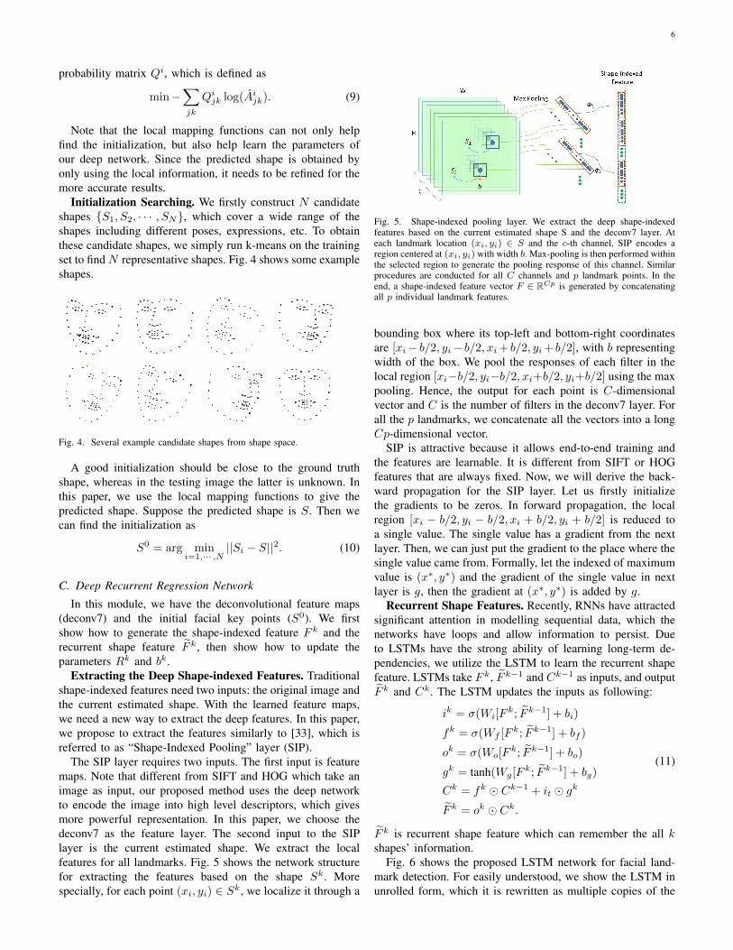
Extracting the Deep Shape-indexed Features. Traditionalshape-indexed features need two inputs: the original image andthe current estimated shape. With the learned feature maps,we need a new way to extract the deep features. In this paper,we propose to extract the features similarly to [33], which isreferred to as “Shape-Indexed Pooling” layer (SIP).

The SIP layer requires two inputs. The first input is featuremaps. Note that different from SIFT and HOG which take animage as input, our proposed method uses the deep networkto encode the image into high level descriptors, which givesmore powerful representation. In this paper, we choose thedeconv7 as the feature layer. The second input to the SIPlayer is the current estimated shape. We extract the localfeatures for all landmarks. Fig. 5 shows the network structurefor extracting the features based on the shape Sk. Morespecially, for each point (xi, yi) ∈ Sk, we localize it through a

Fig. 5. Shape-indexed pooling layer. We extract the deep shape-indexedfeatures based on the current estimated shape S and the deconv7 layer. Ateach landmark location (xi, yi) ∈ S and the c-th channel, SIP encodes aregion centered at (xi, yi) with width b. Max-pooling is then performed withinthe selected region to generate the pooling response of this channel. Similarprocedures are conducted for all C channels and p landmark points. In theend, a shape-indexed feature vector F ∈ RCp is generated by concatenatingall p individual landmark features.

bounding box where its top-left and bottom-right coordinatesare [xi− b/2, yi− b/2, xi+ b/2, yi+ b/2], with b representingwidth of the box. We pool the responses of each filter in thelocal region [xi−b/2, yi−b/2, xi+b/2, yi+b/2] using the maxpooling. Hence, the output for each point is C-dimensionalvector and C is the number of filters in the deconv7 layer. Forall the p landmarks, we concatenate all the vectors into a longCp-dimensional vector.

SIP is attractive because it allows end-to-end training andthe features are learnable. It is different from SIFT or HOGfeatures that are always fixed. Now, we will derive the back-ward propagation for the SIP layer. Let us firstly initializethe gradients to be zeros. In forward propagation, the localregion [xi − b/2, yi − b/2, xi + b/2, yi + b/2] is reduced toa single value. The single value has a gradient from the nextlayer. Then, we can just put the gradient to the place where thesingle value came from. Formally, let the indexed of maximumvalue is (x∗, y∗) and the gradient of the single value in nextlayer is g, then the gradient at (x∗, y∗) is added by g.

Recurrent Shape Features. Recently, RNNs have attractedsignificant attention in modelling sequential data, which thenetworks have loops and allow information to persist. Dueto LSTMs have the strong ability of learning long-term de-pendencies, we utilize the LSTM to learn the recurrent shapefeature. LSTMs take F k, F k−1 and Ck−1 as inputs, and outputF k and Ck. The LSTM updates the inputs as following:

ik = σ(Wi[Fk; F k−1] + bi)

fk = σ(Wf [F k; F k−1] + bf )

ok = σ(Wo[Fk; F k−1] + bo)

gk = tanh(Wg[Fk; F k−1] + bg)

Ck = fk � Ck−1 + it � gk

F k = ok � Ck.

(11)

F k is recurrent shape feature which can remember the all kshapes’ information.

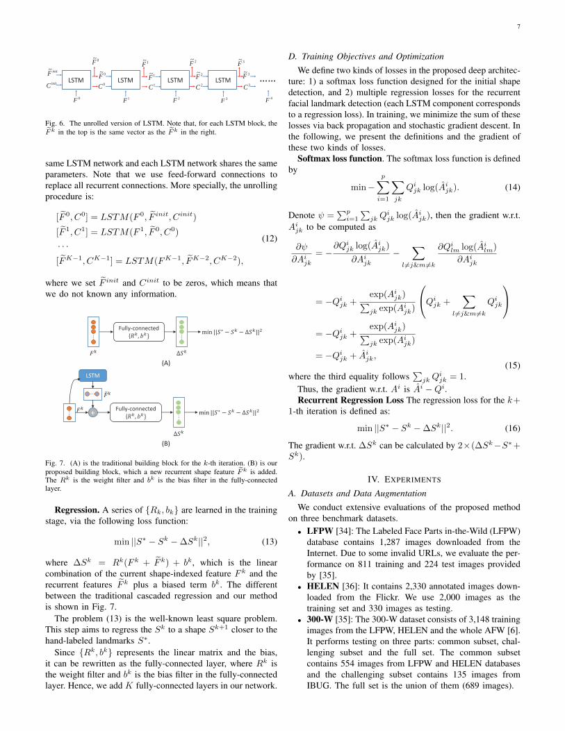
Fig. 6 shows the proposed LSTM network for facial land-mark detection. For easily understood, we show the LSTM inunrolled form, which it is rewritten as multiple copies of the

7

LSTM LSTM LSTM LSTM

0F

0~F

……initF~

initC

0~F0C

1~F1C

2~F2C

3~F3C

1F 2F 3F 4F

1~F 2~F 3~F

Fig. 6. The unrolled version of LSTM. Note that, for each LSTM block, theFk in the top is the same vector as the Fk in the right.

same LSTM network and each LSTM network shares the sameparameters. Note that we use feed-forward connections toreplace all recurrent connections. More specially, the unrollingprocedure is:

[F 0, C0] = LSTM(F 0, F init, Cinit)

[F 1, C1] = LSTM(F 1, F 0, C0)

· · ·[FK−1, CK−1] = LSTM(FK−1, FK−2, CK−2),

(12)

where we set F init and Cinit to be zeros, which means thatwe do not known any information.

LSTM

+…

…Fully-connected

{… …

(A)

Fully-connected { …

(B)

Fig. 7. (A) is the traditional building block for the k-th iteration. (B) is ourproposed building block, which a new recurrent shape feature Fk is added.The Rk is the weight filter and bk is the bias filter in the fully-connectedlayer.

Regression. A series of {Rk, bk} are learned in the trainingstage, via the following loss function:

min ||S∗ − Sk −∆Sk||2, (13)

where ∆Sk = Rk(F k + F k) + bk, which is the linearcombination of the current shape-indexed feature F k and therecurrent features F k plus a biased term bk. The differentbetween the traditional cascaded regression and our methodis shown in Fig. 7.

The problem (13) is the well-known least square problem.This step aims to regress the Sk to a shape Sk+1 closer to thehand-labeled landmarks S∗.

Since {Rk, bk} represents the linear matrix and the bias,it can be rewritten as the fully-connected layer, where Rk isthe weight filter and bk is the bias filter in the fully-connectedlayer. Hence, we add K fully-connected layers in our network.

D. Training Objectives and Optimization

We define two kinds of losses in the proposed deep architec-ture: 1) a softmax loss function designed for the initial shapedetection, and 2) multiple regression losses for the recurrentfacial landmark detection (each LSTM component correspondsto a regression loss). In training, we minimize the sum of theselosses via back propagation and stochastic gradient descent. Inthe following, we present the definitions and the gradient ofthese two kinds of losses.

Softmax loss function. The softmax loss function is definedby

min−p∑i=1

∑jk

Qijk log(Aijk). (14)

Denote ψ =∑pi=1

∑jkQ

ijk log(Aijk), then the gradient w.r.t.

Aijk to be computed as

∂ψ

∂Aijk= −

∂Qijk log(Aijk)

∂Aijk−

∑l 6=j&m6=k

∂Qilm log(Ailm)

∂Aijk

= −Qijk +exp(Aijk)∑jk exp(Aijk)

Qijk +∑

l 6=j&m6=k

Qijk

= −Qijk +

exp(Aijk)∑jk exp(Aijk)

= −Qijk + Aijk,(15)

where the third equality follows∑jkQ

ijk = 1.

Thus, the gradient w.r.t. Ai is Ai −Qi.Recurrent Regression Loss The regression loss for the k+

1-th iteration is defined as:

min ||S∗ − Sk −∆Sk||2. (16)

The gradient w.r.t. ∆Sk can be calculated by 2×(∆Sk−S∗+Sk).

IV. EXPERIMENTS

A. Datasets and Data Augmentation

We conduct extensive evaluations of the proposed methodon three benchmark datasets.• LFPW [34]: The Labeled Face Parts in-the-Wild (LFPW)

database contains 1,287 images downloaded from theInternet. Due to some invalid URLs, we evaluate the per-formance on 811 training and 224 test images providedby [35].

• HELEN [36]: It contains 2,330 annotated images down-loaded from the Flickr. We use 2,000 images as thetraining set and 330 images as testing.

• 300-W [35]: The 300-W dataset consists of 3,148 trainingimages from the LFPW, HELEN and the whole AFW [6].It performs testing on three parts: common subset, chal-lenging subset and the full set. The common subsetcontains 554 images from LFPW and HELEN databasesand the challenging subset contains 135 images fromIBUG. The full set is the union of them (689 images).

8

We conduct evaluations on 68 points (provided by [35]) onthe LFPW, HELEN and 300-W datasets.

Data augmentation. We train our models only using thedata from the training data without external sources. To reduceoverfitting on the training data, we employ three distinct formsof data augmentation to artificially enlarge the dataset.

The first form of data augmentation is to generate imagerotations. We do this by rotating the image into different anglesincluding {±30,±25,±20,±15,±10,±5, 0}.

The second form of data augmentation is to disturb thebounding boxes, which can increase the robustness of ourresults to the bounding boxes. We randomly scale and translatethe bounding box for each image.

The third form of data augmentation is mirroring. We flipall images and their shapes.

After the data augmentation, the number of training samplesis enlarged to 52 times, which is shown in Table I.

TABLE ITHE NUMBER OF TRAINING SAMPLES AFTER DATA AUGMENTATION.

LFPW HELEN 300-W42,172 121,160 163,696

B. Experimental Setting

Implementation details. We implement the proposedmethod based on the open source Caffe [37] framework, whichis an efficient deep neural network implementation. Note thatthe Caffe also includes the implement of the LSTM layer 3.We first crop the image using the bounding box with the0.2W padding on all sides (top, bottom, left, right), whereW is the width of the bounding box. We scale the longestside to 256 leaving us with a 256 × H or H × 256 sizedimage, where H ≤ 256. Then we add zeros to the smallestside and make the size of 256 × 256 pixels. The numberof candidate shapes is set to N = 50. We set K = 8 andb = 6. Our network is trained by stochastic gradient descentwith 0.9 momentum. The weight decay parameter is 0.0001.The network’s parameters are initialized with the pre-trainedVGG19 model.

Evaluation. We evaluate the alignment accuracies by twopopular metrics, the mean error and the cumulative errors. Themean error is measured by the distances between the predictedlandmarks and the ground truths, normalized by the inter-pupildistance, which can be calculated by

mean error =1

n

n∑i=1

||Si − S∗i ||2

pDi(17)

where Si is the predicted shape and S∗i is the ground-truthshape for the i-th image. Di is the distance between two eyes.p is the number of landmarks and n is the total number offace images.

We also report the cumulative errors distribution (CED)curve, in which the mean error larger than l is reported as a

3https://github.com/LisaAnne/lisa-caffe-public/tree/lstm video deploy

failure. Let ei =||Si−S∗i ||

2

pDi, and CED at the error l is defined

as

CED =Ne≤ln

, (18)

where Ne≤l is the number of images on which the error ei isno higher than l.

C. Comparison with State-of-the-art Algorithms

The first set of experiments is to evaluate the performanceof the proposed method and compare it with several state-of-the-art algorithms. Zhu et al. [6], DRMF [38], ESR [8],RCPR [24], SDM [9], Smith et al. [32], Zhao et al. [39], GN-DPM [40], CFAN [20], ERT [41], LBF [13], cGPRT [11],CFSS [12] and TCDCN [42] are selected as the baselines.

1) Comparison on LFPW: The goal of LFPW is to evaluatethe facial landmark detection algorithms under unconstrainedconditions. The images include different poses, expressions,illuminations and occlusions, and mainly are collected fromthe Internet.

TABLE IIMEAN ERROR ON LFPW DATASET.

LFPW DatasetMethods 68 pts

Zhu et al. 8.29DRMF 6.57RCPR 5.67SDM 5.67

GN-DPM 5.92CFAN 5.44CFSS 4.87

CFSS Practical 4.90OURS 4.49

We compare the proposed method with the several state-of-the-art methods as shown in Table II. As can be seen,the proposed deep-network based facial landmark detectionis significantly better than the baselines. The most similarwork is SDM which is also a cascaded regression method.The main different is that it is trained by the hand-craftedfeatures. The mean error of SDM is 5.67, while the proposedmethod is 4.49. CFSS is the recent proposed method, whichachieves an excellent performance on this dataset. Even so,our method also performances better that CFSS, and showsan error reduction of 0.38.

2) Comparison on HELEN: The images of HELEN aredownloaded from Flickr, which under a broad range of ap-pearance variation, including lighting, individual differences,occlusion and pose. The HELEN dataset contains many suffi-ciently large faces (greater than 500 pixels in width) and canfit accurately for high resolution images.

Table III shows the comparison results of mean error on theHELEN dataset. The comparison shows our proposed methodcan achieve better results than the baselines. For example, themean error of our method is 4.02, compared to the 4.60 of thesecond best algorithm.

9

TABLE IIIMEAN ERROR ON HELEN DATABASE.

Helen DatasetMethods 68 pts

Zhu et al. 8.16DRMF 6.70

ESR 5.70RCPR 5.93SDM 5.50

GN-DPM 5.69CFAN 5.53CFSS 4.63

CFSS Practical 4.72TCDCN 4.60OURS 4.02

TABLE IVMEAN ERROR ON 300W DATABASE.

300-W DatasetMethods Common Challenging Fullset

Zhu et al. 8.22 18.33 10.20DRMF 6.65 19.79 9.22

ESR 5.28 17.00 7.58RCPR 6.18 17.26 8.35SDM 5.57 15.40 7.50

Smith et al. 13.30Zhao et al. 6.31GN-DPM 5.78

CFAN 5.50ERT 6.40LBF 4.95 11.98 6.32

LBF fast 5.38 15.50 7.37cGPRT 5.71CFSS 4.73 9.98 5.76

CFSS Practical 4.79 10.92 5.99TCDCN 4.80 8.60 5.54OURS 4.07 8.29 4.90

3) Comparison on 300W: The 300W is extremely chal-lenging dataset, which is widely used for comparing the per-formance of different algorithms of facial landmark detectionunder the same evaluation protocol.

Table IV shows the comparison results of mean error on the300W dataset. It can be observed that the proposed methodperforms significantly better than all previous methods in allsettings. Specifically, on Fullset, our method obtains a meanerror of 4.90, which gives an error reduction of 0.64 comparedto the second best algorithm. On Challenging, our methodshows an error reduction of 0.31 in comparison with thesecond best method. On Common, the mean error of ourmethod is 4.07, compared to 4.73 of the second best algorithm.

Fig. 8 shows the CED curves for different error levels on the300-W dataset. Again, for all error levels, our method yieldsthe highest accuracy and beats all the baselines. For instance,the proposed method shows a relative increase of 23% on the300w common set compared to the second best algorithm. Theexample alignment results of our method are shown in TableV and Table VI.

One main reason for the good performance of our methodis that instead of using traditional hand-crafted visual features(SIFT, HOG), it uses the deep network to learn the image

Mean Localisation Error / Inter-pupil Distance0 5 10 15

Fra

ctio

n of

Tes

t Fac

es (

554

in T

otal

)

0

0.1

0.2

0.3

0.4

0.5

0.6

0.7

0.8

0.9

1CED for 68-pts common subset of 300-W

Zhu et alDRMFRCPRSDMGN-DPMCFANCFSS PraticalOURS

Fig. 8. CED curves on common subset of 300-W.

Mean Localisation Error / Inter-pupil Distance0 5 10 15 20 25 30

Fra

ctio

n of

Tes

t Fac

es (

135

in T

otal

)

0

0.1

0.2

0.3

0.4

0.5

0.6

0.7

0.8

0.9

1CED for 68-pts challenging subset of 300-W

Zhu et alDRMFRCPRSDMSmith et alCFSS PraticalOURS

Fig. 9. CED curves on challenging subset of 300-W.

representations and extracts the deep shape-indexed features.Second, our method can incorporate the previous shape in-formation to the current shape regression, which can help toobtain a good performance.

D. Further Analyses

1) Effects of Different Input Sizes and Networks: Some mayargue that our network is too large and deep, it may impracticalto be used. Since the most time consuming module is thespatial resolution-preserved network, we explore the effects ofdifferent sub-networks in this subsection. Also the input sizeof image can effect the running time, e.g., the running time of128× 128’s image is 4 times faster than that of 256× 256’s.Hence, we also explore the effects of different sizes of inputimages.

We show the results of two different types of frameworks:VGG-S 4 and VGG-19, where VGG-S is a small convolutionalneural network and it only has five convolutional layers. Notethat same modifications are made on the two frameworks asdescribed above (i.e., removing all the fully-connected layers,keeping the first two pooling layers, other pooling layers are

4https://github.com/BVLC/caffe/wiki/Model-Zoo

10

TABLE VSHAPE DETECTION EXAMPLES FROM 300W COMMON SUBSET.

TABLE VISHAPE DETECTION EXAMPLES FROM 300W CHALLENGE SUBSET.

TABLE VIICONFIGURATIONS OF THE SPATIAL RESOLUTION-PRESERVED

CONV-DECONV NETWORK FOR VGG-S WITH THE INPUT SIZE :256× 256.

type filter size/stride/pad output sizeconv1 7 × 7 / 1 / 3 96 × 256 × 256

max pool1 2 × 2 / 2 / 0 96 × 128 × 128conv2 5× 5 / 1 / 2 256 × 128 × 128

max pool2 2 × 2 / 2 / 0 256 × 64 × 64conv3 3× 3 / 1 / 1 512 × 64 × 64conv4 3× 3 / 1 / 1 512 × 64 × 64conv5 3× 3 / 1 / 1 512 × 64 × 64

deconv6 4× 4 / 2 / 1 96 × 128 × 128deconv7 4× 4 / 2 / 1 96 × 256 × 256

removed and adding two deconvolutional layers). After themodification, it has five convolutional layers, two max poolinglayers and two deconvolutional layers. Table. VII shows thenetwork architecture of VGG-S. Compared to VGG-19, VGG-

S is a very small network. This set of experiments is to showus that whether our method can performs well in the smallnetwork. We also report the results with two different inputsizes: 256× 256 and 128× 128.

Table VIII shows the comparison results, from which it canbe seen that: our method can perform well even using verysmall sub-network. For example, the mean error of fullsetis 4.90 when the sub-network is VGG-19, compared to 5.01when the sub-network is VGG-S. Note that the mean errorof TCDCN is 5.54, which is the second best results on TableIV. The mean error of challenging is 8.29 when the inputsize is 256 × 256, compared to 8.80 when the input size is128 × 128. The results are not surprising since it is hardto discriminate the key facial points in the small images.The results also show that keeping the spatial information isimportant. In summary, our framework is capable of exploitingdifferent types of characteristics, i.e., accuracy or speed, byusing different sub-networks or different input sizes.

11

TABLE VIIIMEAN ERRORS ON DIFFERENT NETWORKS AND DIFFERENT INPUT SIZES.

300-WCommon Challenging Fullset

VGG-S (128x128) 4.62 9.01 5.48VGG-S (256x256) 4.22 8.23 5.01VGG-19 (128x128) 4.57 8.80 5.40VGG-19 (256x256) 4.07 8.29 4.90

2) Effects of the Recurrent Shape Features: In our secondset of experiments, we evaluate the advantages of the proposedrecurrent shape features in our framework. To make a faircomparison, we compare two methods:• facial landmark detection with recurrent shape fea-

tures. We use the recurrent shape features in our networkas shown in Fig. 7 (B).

• facial landmark detection without recurrent shapefeatures. The facial landmark detection is learned withoutthe assistance of the recurrent shape features, i.e., onlyuse the shape-indexed features as shown in Fig. 7 (A).

Since the two methods use the same network and the onlydifferent is that using or not using the recurrent shape features,these comparisons can show us whether the recurrent shapefeatures can contribute to the accuracy or not.

TABLE IXMEAN ERRORS ON 300-W DATASET.

Common Challenging FullsetVGG-S (128x128)

without recurrent features 5.19 9.75 6.08with recurrent features 4.62 9.01 5.48

VGG-S (256x256)without recurrent features 4.51 9.64 5.51

with recurrent features 4.22 8.23 5.01VGG-19 (128x128)

without recurrent features 4.81 9.22 5.67with recurrent features 4.57 8.80 5.40

VGG-19 (256x256)without recurrent features 4.19 8.42 5.02

with recurrent features 4.07 8.29 4.90

Table IX shows the comparison results with respect to MeanErrors. The results show that our proposed recurrent shapefeatures can achieve better performance than the baseline thatare without recurrent shape features, especially for the smallnetwork (VGG-S). For instance, the mean errors of fullset is5.48 when the sub-network is VGG-S and the image size is128×128, compared to 6.08 of the baseline. The main reasonis that the proposed features can learn the temporal dynamicsinformation.

TABLE XCOMPARISON WITH MEAN SHAPE INITIALISATION.

300-WCommon Challenging Fullset

Mean Shape 4.31 8.29 5.08N = 50 4.07 8.29 4.90N = 500 4.06 8.29 4.89

N = 5000 4.07 8.32 4.91

(A) The first stage

256

256

SIP

+…

…

…

(B) The second stage

LSTM

+…

…

+

SIP

LSTM

+…

…

SIP

LSTM

+…

…

+

Memory Cell:

Regression Regression Regression

…

conv5conv1 conv2 deconv6 deconv7

96

256

256

96

128

128

64

64128

128256

256

68

256

256

…

conv8

deconv7

Fig. 10. The two-stage learning strategy.

3) Effects of the Local Mapping Functions: In this setof experiments, we show the advantages of the proposedlocal mapping functions. To give an intuitive comparison, wecompare with the mean shape initialization setting as shown inFig. 1. We use the same network and same cascade regressions.The only different is that we use the mean shape as theinitialisation instead of using the local mapping functions tosearch the initialisation. These comparisons can answer uswhether the proposed local mapping functions can contributeto improve the accuracy or not. We also added experiments toexplore the effect of different number of candidate shapes N .

Table X show the comparison results. The results showthat the proposed local mapping functions perform better thatthe mean shape. There are two main reasons for the goodperformance. First, we learn local mapping functions togetherwith the cascaded regression, which means two correlatedtasks are learned together. Zhang et al. [43] had showed thatleaning related tasks can improve the detection robustness.The second reason is that our method can find the betterinitialisation.

The results in Table X also show that the method using N =50 candidate shapes performs close to those using N = 500or N = 5000 shapes. Thus, we simply use N = 50 candidateshapes in this paper.

Note that different with the CFSS method which the goodinitialisation performs significantly better than the mean shapeinitialisation, our method is not sensitize to the initialisationand performs more stable. The reason maybe that the proposedrecurrent shape features can keep the previous information andhelp to be more robust to the initialization.

4) Effect of the End-to-end Learning: Our framework is anend-to-end framework. To show the advantages of the end-to-end framework, we compare to the following baselines.The first baseline is SDM [9]. SDM is a traditional cascadedregression method, which is not an end-to-end framework.The second baseline also uses our framework but adopts atwo-stage strategy. We divide our framework into two partsaccording to the pipeline of the traditional cascaded regres-sion methods: (1) visual features are first extracted; (2) theestimated shapes are then updated via regression from theextracted features; In the first stage, we learn the visual featureas shown in the Fig. 10 (a). In the second stage, we learn the

12

regression via the visual features as shown in Fig. 10 (b). Notethat the deconv7 is fixed in the second stage.

TABLE XICOMPARISON WITH THE NON END-TO-END METHODS.

300-WCommon Challenging Fullset

SDM 5.57 15.40 7.50Two-stage 4.64 8.91 5.47

OURS 4.07 8.29 4.90

Table XI shows the comparison results. We can observe thatthe two-stage method performs better that the SDM, and ourone-stage method performs better than the two-stage method.It is desirable to learn the whole facial landmark detectionprocess in the end-to-end framework.

5) Effects of the Number of Regressions: In this paper, weuse K = 8 regressions. Table XII shows the mean errors ofall these regressions. We can see that the results are very closeto each other after 4 steps. K = 8 used in this paper is largerenough to let our method converges.

TABLE XIIEFFECTS OF THE NUMBER OF REGRESSIONS.

300-WCommon Challenging Fullset

Step 1 4.77 9.72 5.74Step 2 4.21 8.69 5.08Step 3 4.10 8.40 4.94Step 4 4.08 8.33 4.91Step 5 4.08 8.31 4.91Step 6 4.07 8.30 4.90Step 7 4.07 8.29 4.90Step 8 4.07 8.29 4.90

6) Comparison Results of 5-point Facial Landmark De-tection: The proposed method can be use predict differentnumber of facial landmarks, e.g., 68 landmark points or 5landmark points. In order to conduct comparisons with moredeep-networks-based methods, we evaluate the performanceof the proposed method on datasets of 5-point facial landmarkdetection.

We conduct experiments on the Multi-Attribute Facial Land-mark (MAFL) dataset. MAFL contains 20,000 facial imagesrandomly chosen from the Celebrity face dataset [44], eachimage has a 5-point landmark annotation. Following the settingof [42], 1, 000 faces are used as the test set, and the rest imagesare used as the training set.

TABLE XIIICOMPARISON RESULTS W.R.T. MEAN ERROR ON THE MAFL DATASET.

MAFLMethods 5 ptsCFAN 15.84

Cascaded CNN 9.73TCDCN 7.95OURS 4.51

Three deep-networks-based methods are used as the base-lines: CFAN [20], Cascaded CNN [18] and TCDCN [42].

Table XIII shows the comparison results w.r.t. the mean erroron the MAFL dataset. We can see that, in the 5-point faciallandmark detection, the proposed method performs better thanthe deep-networks-based baselines.

7) Effect of Incorporating Shallower-Layer Features: Inthe proposed method, we use deconv7 layer as input to theSIP layer to extract deep shape-indexed features. A naturalquestion arising here is whether we can combine deconv7with the shallower-layer features. To answer this question,we evaluate the performance of different variants of theproposed method. In each variant, we use conv5, deconv6,deconv7, conv5 combined with deconv7, deconv6 combinedwith deconv7 as the input to the SIP layer for extracting deepshape-indexed features, respectively. The comparison resultsw.r.t. mean error on the 300-W dataset are shown in TableXIV. We can see that combining deconv7 with shallower-layers’ features can slightly improve the performance. Forexample, the mean error of the variant that combines deconv6and deconv7 is 4.85, compared to the 4.90 of the method thatonly uses deconv7.

TABLE XIVCOMPARISON RESULTS W.R.T. MEAN ERROR ON 300-W.

300-WCommon Challenging Fullset

conv5 4.21 8.30 5.01deconv6 4.09 8.06 4.87deconv7 4.07 8.29 4.90

conv5 + deconv7 4.11 8.05 4.88deconv6 + deconv7 4.08 8.01 4.85

V. CONCLUSIONS

In this paper, we proposed an end-to-end deep-network-based cascaded regression method for facial landmark detec-tion. In the proposed deep architecture, an input image is firstlyencoded into high level descriptors in the same size of theinput image. Based on this representation, we proposed tolearn a probability map for each facial key point and use theseprobability maps to find the initialization for the cascadedregression. And then, we proposed two strong features. Oneis the deep shape-indexed features, which are extracted by thedesigned shape-indexed pooling layer. Another is the recurrentshape features, which is used to learn the connection betweenthe regressions. Finally, the sequential linear regressions arelearned to update the shapes. Empirical evaluations on threedatasets show that the proposed method significantly outper-forms the state-of-the-arts.

REFERENCES

[1] W. Zhao, R. Chellappa, P. J. Phillips, and A. Rosenfeld, “Face recogni-tion: A literature survey,” ACM Computing Surveys, vol. 35, no. 4, pp.399–458, 2003.

[2] L. Liu, J. Xing, S. Liu, H. Xu, X. Zhou, and S. Yan, “Wow! youare so beautiful today!” ACM Transactions on Multimedia Computing,Communications, and Applications, vol. 11, no. 1s, p. 20, 2014.

[3] I. Kemelmacher-Shlizerman, S. Suwajanakorn, and S. M. Seitz,“Illumination-aware age progression,” in IEEE Conference on ComputerVision and Pattern Recognition, 2014, pp. 3334–3341.

13

[4] C. Cao, Q. Hou, and K. Zhou, “Displaced dynamic expression regressionfor real-time facial tracking and animation,” ACM Transactions onGraphics, vol. 33, no. 4, p. 43, 2014.

[5] J. M. Saragih, S. Lucey, and J. F. Cohn, “Deformable model fitting byregularized landmark mean-shift,” International Journal of ComputerVision, vol. 91, no. 2, pp. 200–215, 2011.

[6] X. Zhu and D. Ramanan, “Face detection, pose estimation, and landmarklocalization in the wild,” in IEEE Conference on Computer Vision andPattern Recognition, 2012, pp. 2879–2886.

[7] P. Martins, R. Caseiro, and J. Batista, “Generative face alignmentthrough 2.5 d active appearance models,” Computer Vision and ImageUnderstanding, vol. 117, no. 3, pp. 250–268, 2013.

[8] X. Cao, Y. Wei, F. Wen, and J. Sun, “Face alignment by explicit shaperegression,” International Journal of Computer Vision, vol. 107, no. 2,pp. 177–190, 2014.

[9] X. Xiong and F. De la Torre, “Supervised descent method and itsapplications to face alignment,” in IEEE Conference on Computer Visionand Pattern Recognition, 2013, pp. 532–539.

[10] P. Dollar, P. Welinder, and P. Perona, “Cascaded pose regression,” inIEEE Conference on Computer Vision and Pattern Recognition, 2010,pp. 1078–1085.

[11] D. Lee, H. Park, and C. D. Yoo, “Face alignment using cascade gaussianprocess regression trees,” in IEEE Conference on Computer Vision andPattern Recognition, 2015, pp. 4204–4212.

[12] S. Zhu, C. Li, C. C. Loy, and X. Tang, “Face alignment by coarse-to-fineshape searching,” in IEEE Conference on Computer Vision and PatternRecognition, 2015, pp. 4998–5006.

[13] S. Ren, X. Cao, Y. Wei, and J. Sun, “Face alignment at 3000 fpsvia regressing local binary features,” in IEEE Conference on ComputerVision and Pattern Recognition, 2014, pp. 1685–1692.

[14] B. Martinez, M. F. Valstar, X. Binefa, and M. Pantic, “Local evidenceaggregation for regression-based facial point detection,” IEEE Transac-tions on Pattern Analysis and Machine Intelligence, vol. 35, no. 5, pp.1149–1163, 2013.

[15] X. Gao, Y. Su, X. Li, and D. Tao, “A review of active appearancemodels,” IEEE Transactions on Systems, Man, and Cybernetics, Part C:Applications and Reviews, vol. 40, no. 2, pp. 145–158, 2010.

[16] N. Wang, X. Gao, D. Tao, and X. Li, “Facial feature point detection: Acomprehensive survey,” arXiv preprint arXiv:1410.1037, 2014.

[17] X. Xiong and F. De la Torre, “Global supervised descent method,” inIEEE Conference on Computer Vision and Pattern Recognition, 2015,pp. 2664–2673.

[18] Y. Sun, X. Wang, and X. Tang, “Deep convolutional network cascadefor facial point detection,” in IEEE Conference on Computer Vision andPattern Recognition, 2013, pp. 3476–3483.

[19] Q. Liu, J. Deng, and D. Tao, “Dual sparse constrained cascade regressionfor robust face alignment,” IEEE Transactions on Image Processing,2016.

[20] J. Zhang, S. Shan, M. Kan, and X. Chen, “Coarse-to-fine auto-encodernetworks (cfan) for real-time face alignment,” in European Conferenceon Computer Vision, 2014, pp. 1–16.

[21] J. Zhang, M. Kan, S. Shan, X. Zhao, and X. Chen, “Topic-awaredeep auto-encoders (tda) for face alignment,” in Asian Conference onComputer Vision. Springer, 2014, pp. 703–718.

[22] J. Zhang, M. Kan, S. Shan, and X. Chen, “Leveraging datasets withvarying annotations for face alignment via deep regression network,” inIEEE International Conference on Computer Vision, 2015, pp. 3801–3809.

[23] S. Belharbi, C. Chatelain, R. Herault, and S. Adam, “Facial landmarkdetection using structured output deep neural networks,” arXiv preprintarXiv:1504.07550, 2015.

[24] X. P. Burgos-Artizzu, P. Perona, and P. Dollar, “Robust face landmarkestimation under occlusion,” in IEEE International Conference on Com-puter Vision, 2013, pp. 1513–1520.

[25] A. Graves and N. Jaitly, “Towards end-to-end speech recognition withrecurrent neural networks,” in International Conference on MachineLearning, 2014, pp. 1764–1772.

[26] O. Vinyals, A. Toshev, S. Bengio, and D. Erhan, “Show and tell: Aneural image caption generator.” arXiv preprint arXiv:1411.4555, 2014.

[27] J. Donahue, L. A. Hendricks, S. Guadarrama, M. Rohrbach, S. Venu-gopalan, T. Darrell, and K. Saenko, “Long-term recurrent convolutionalnetworks for visual recognition and description,” in IEEE Conferenceon Computer Vision and Pattern Recognition, 2015, pp. 2625–2634.

[28] X. Peng, R. S. Feris, X. Wang, and D. N. Metaxas, “A recurrent encoder-decoder network for sequential face alignment,” in European Conferenceon Computer Vision. Springer, 2016, pp. 38–56.

[29] K. Simonyan and A. Zisserman, “Very deep convolutional networks forlarge-scale image recognition,” arXiv preprint arXiv:1409.1556, 2014.

[30] J. Long, E. Shelhamer, and T. Darrell, “Fully convolutional networksfor semantic segmentation,” arXiv preprint arXiv:1411.4038, 2014.

[31] H. Noh, S. Hong, and B. Han, “Learning deconvolution network forsemantic segmentation,” arXiv preprint arXiv:1505.04366, 2015.

[32] B. M. Smith, J. Brandt, Z. Lin, and L. Zhang, “Nonparametric contextmodeling of local appearance for pose-and expression-robust faciallandmark localization,” in IEEE Conference on Computer Vision andPattern Recognition, 2014, pp. 1741–1748.

[33] K. He, X. Zhang, S. Ren, and J. Sun, “Spatial pyramid pooling in deepconvolutional networks for visual recognition,” in European Conferenceon Computer Vision, 2014, pp. 346–361.

[34] P. N. Belhumeur, D. W. Jacobs, D. J. Kriegman, and N. Kumar,“Localizing parts of faces using a consensus of exemplars,” IEEETransactions on Pattern Analysis and Machine Intelligence, vol. 35,no. 12, pp. 2930–2940, 2013.

[35] C. Sagonas, G. Tzimiropoulos, S. Zafeiriou, and M. Pantic, “300 facesin-the-wild challenge: The first facial landmark localization challenge,”in IEEE International Conference on Computer Vision Workshops, 2013,pp. 397–403.

[36] V. Le, J. Brandt, Z. Lin, L. Bourdev, and T. S. Huang, “Interactive facialfeature localization,” in European Conference on Computer Vision, 2012,pp. 679–692.

[37] Y. Jia, “Caffe: An open source convolutional architecture for fast featureembedding,” http://caffe.berkeleyvision.org, 2013.

[38] A. Asthana, S. Zafeiriou, S. Cheng, and M. Pantic, “Robust discrim-inative response map fitting with constrained local models,” in IEEEConference on Computer Vision and Pattern Recognition, 2013, pp.3444–3451.

[39] X. Zhao, T.-K. Kim, and W. Luo, “Unified face analysis by iterativemulti-output random forests,” in IEEE Conference on Computer Visionand Pattern Recognition, 2014, pp. 1765–1772.

[40] G. Tzimiropoulos and M. Pantic, “Gauss-newton deformable part modelsfor face alignment in-the-wild,” in IEEE Conference on Computer Visionand Pattern Recognition, 2014, pp. 1851–1858.

[41] V. Kazemi and J. Sullivan, “One millisecond face alignment with anensemble of regression trees,” in IEEE Conference on Computer Visionand Pattern Recognition, 2014, pp. 1867–1874.

[42] Z. Zhang, P. Luo, C. C. Loy, and X. Tang, “Learning deep representationfor face alignment with auxiliary attributes,” IEEE Transactions onPattern Analysis and Machine Intelligence, 2015.

[43] Z. Zhang, P. Luo, C. Chen, and X. Tang, “Facial landmark detection bydeep multi-task learning,” in European Conference on Computer Vision,2014, pp. 94–108.

[44] Y. Sun, X. Wang, and X. Tang, “Deep learning face representation frompredicting 10,000 classes,” in IEEE Conference on Computer Vision andPattern Recognition, 2014, pp. 1891–1898.