Embed Size (px)
Citation preview

Deep penetration and total transmission in lossy media
Nicola Tedeschi
LABCEM II

11/11/2016TU1208 Training School in Split 2
Outline
• Inhomogeneous waves at planar interfaces
• Electromagnetic waves penetration in dissipative media
• Deep-penetrating wave
• Deep penetration and Leaky-waves antennas
• Total-transmission in dissipative media
• Conclusions

11/11/2016 3
Homogeneous and inhomogeneous waves
An electromagnetic wave propagating in a free space must respect the dispersion equation:
Where is the propagation vector,
is the wave number,
is the relative permittivity of the material filling the free space.
2
0 rk k k
k
0k
r r rj
0 0 0k
Lossless Media Lossy Media
Homogeneous
Inhomogeneous
0
0
0
β α
0
β α
0
cos
β α
β
βα
βα
βα
TU1208 Training School in Split

11/11/2016 4
Inhomogeneous waves
0
0
β α
0
cos
β αβα βα
0 Lossless Media Lossy Media
2
, are defined by the antenna
2
2
0
2
0
1 12 cos
1 12 cos
r r
r
r r
r
k
k
TU1208 Training School in Split

11/11/2016 5
GPR antennas
TU1208 Training School in Split
Dipole antenna
Bow-tie antenna Patch antenna
Loop antenna

11/11/2016 6
Transmission in dissipative media
As it is well known, when a homogeneous electromagnetic wave, from a lossless medium, impinges on a
dissipative material, the transmitted wave is attenuated in the direction perpendicular to the planar interface
1 2 2 2j
TU1208 Training School in Split

11/11/2016 7
Transmission of inhomogeneous waves
tα
tβ
t
x
y
t
iαiβ
i
i
1 1 1j 2 2 2j
i i i
t t t
j
j
k β α
k β α
1 0 0
1 0 0
2 0 0
2 0 0
cos sin
cos sin
cos sin
cos sin
i i i
i i i
t t t
t t t
β x y
α x y
β x y
α x y
How can we find the transmitted wave?
From the continuity of the tangential components!
1 2
1 2
sin sin
sin sin
i t
i t
Generalized
Snell condition
TU1208 Training School in Split

11/11/2016 8
Transmission of inhomogeneous waves
tα
tβ
t
x
y
t
iαiβ
i
i
1 1 1j 2 2 2j
i i i
t t t
j
j
k β α
k β α
1 0 0
1 0 0
2 0 0
2 0 0
cos sin
cos sin
cos sin
cos sin
i i i
i i i
t t t
t t t
β x y
α x y
β x y
α x y
How can we find the transmitted wave?
From the continuity of the tangential components!
1 2
1 2
sin sin
sin sin
i t
i t
Generalized
Snell condition
Two equations, four unknowns…we are missing something!
TU1208 Training School in Split

11/11/2016 9
Transmission of inhomogeneous waves (2)
tα
tβ
t
x
y
t
iαiβ
i
i
1 1 1j 2 2 2j
1 2
1 2
sin sin
sin sin
i t
i t
Generalized Snell condition
We have the dispersion equation:
2 2 2
2 2 0 2
2
2 2 2 2 0 22 cos
k
k
Now, with some algebra, we can get the solution:
22 2 2
0 2 2
2
22 2 2
0 2 2
2
2
2
iy iy
iy iy
k k k k
k k k k
Amplitudes of the
transmitted vectors
TU1208 Training School in Split

11/11/2016 10
Angles uncertainty
We know the transmitted amplitudes; we need the transmitted angles.
1
2
1
2
sin sin
sin sin
t i
t i
From the generalized Snell condition:
TU1208 Training School in Split

11/11/2016 11
Angles uncertainty (2)
When we have a doubt, we check the energy conservation!
1 1 1j 2 2 2j
x
y
When the angles come back to 0, the energy does not conserve!
The transmitted angles keep growing after and i
i
TU1208 Training School in Split

11/11/2016 12
Transmitted angles
1
2
1
2
1
2
1
2
arcsin sin with
arcsin sin with
arcsin sin with
arcsin sin with
i i i
t
i i i
i i i
t
i i i
What happens when or ? i i
i i
The, not so simple, expressions of the transmitted angles:
TU1208 Training School in Split

11/11/2016 13
Parallel-phase condition
1 1 1j 2 2 2j
x
y
iα
iβ
tα
tβ
i i
sin 1 2
t t
Let analyse the conditions:
The transmitted wave has
the constant phase plane orthogonal to the interface
The transmitted wave is similar to a surface wave
TU1208 Training School in Split

11/11/2016 14
i i
sin 1 2
t t
Parallel-attenuation condition
1 1 1j 2 2 2j
x
y
iα
iβ
tαtβ
The transmitted wave has
the constant amplitude plane orthogonal to the interface
The transmitted wave is not attenuated
towards the second medium!
This is what we call Deep-penetrating wave
TU1208 Training School in Split

11/11/2016 15
Deep-Penetrating Wave (DPW)
1 1 1j 2 2 2j
x
y
iα
iβ
tαtβ
What a strange behavior! Looking at the radiating power as a function of the deepness, it decays in
the first medium because the losses, but remains constant in the second medium in spite of losses!
TU1208 Training School in Split

11/11/2016 16
Deep-Penetrating Wave (2)
Let now focusing on the case the first medium is lossless.
As we seen in this case we can still have an incident inhomogeneous wave
tα
tβ
t
x
y
t
iα iβ
i
1 2 2 2j
1 2
1 2
sin sin
cos
i t
i
Generalized Snell condition in DPW case
From the dispersion equation:
2
2 2 2 2 0 22 cos k 21 10 2
sin cos2 sin
sin
i it
t
k
2
1 1 0 2sin 2 i k
2
0 2
1 1
1arcsin
2DPW
k
With some algebra:
TU1208 Training School in Split

11/11/2016 17
Deep-Penetrating Wave (3)
TU1208 Training School in Split
At this point, we have an instrument to deeply penetrate in a dissipative medium coming from a lossless
medium, as the air.

11/11/2016 18
Deep-Penetrating Wave (4)
Comparing the magnitude of the Poynting vector of
both the homogeneous and the inhomogeneous wave,
we see:
• A sinusoidal oscillation in the first medium,
because of the reflections;
• A decay of the transmitted power for the
homogeneous incident wave;
• A constant transmitted power for the
inhomogeneous wave
TU1208 Training School in Split
11/11/2016 19
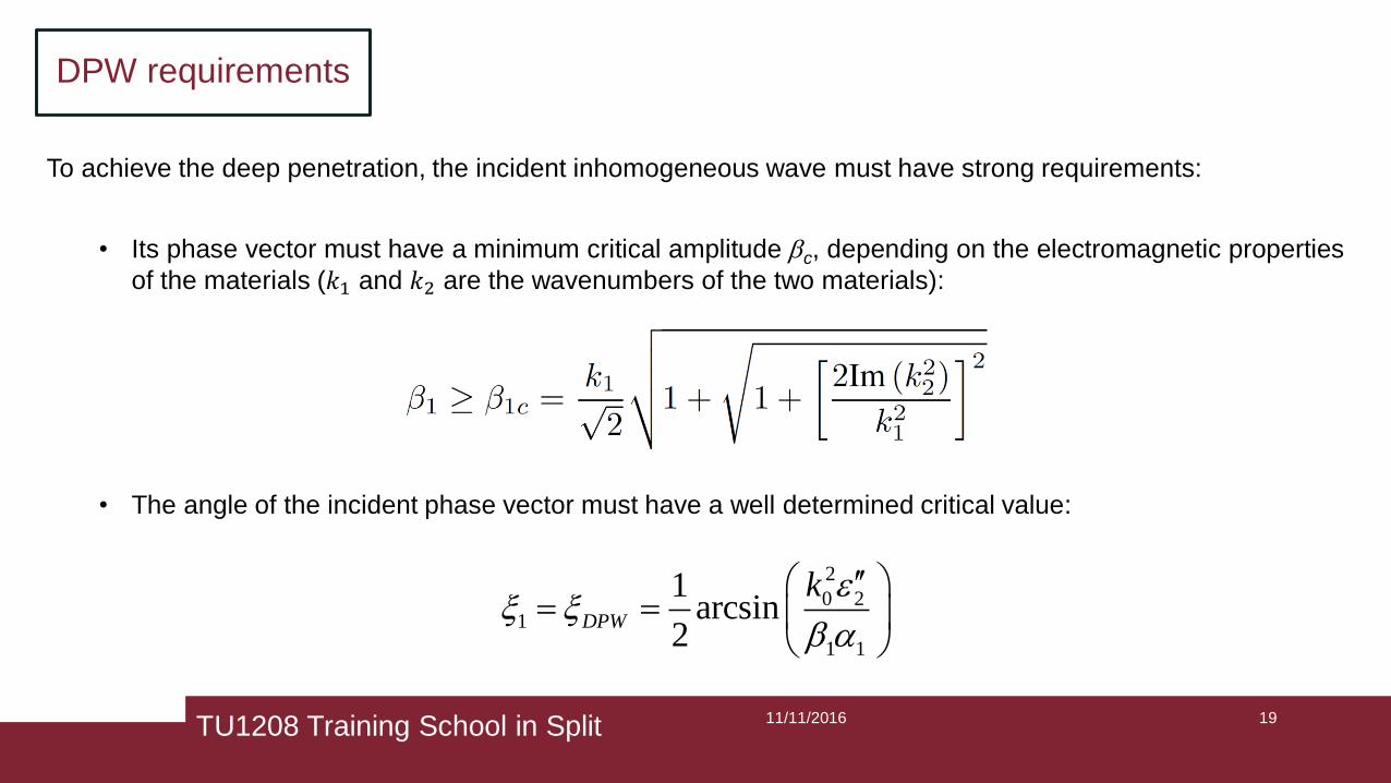
DPW requirements
To achieve the deep penetration, the incident inhomogeneous wave must have strong requirements:
• Its phase vector must have a minimum critical amplitude c, depending on the electromagnetic properties
of the materials (𝑘1 and 𝑘2 are the wavenumbers of the two materials):
• The angle of the incident phase vector must have a well determined critical value:
TU1208 Training School in Split
2
0 21
1 1
1arcsin
2DPW
k
11/11/2016 20
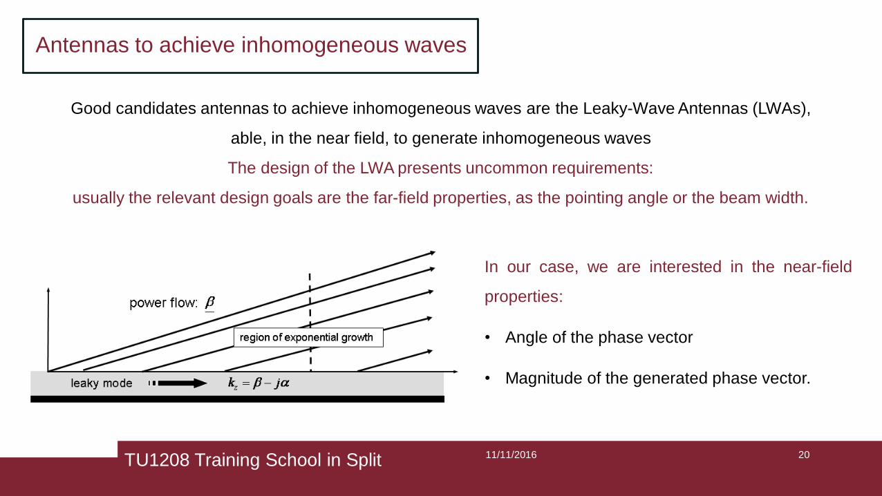
Antennas to achieve inhomogeneous waves
Good candidates antennas to achieve inhomogeneous waves are the Leaky-Wave Antennas (LWAs),
able, in the near field, to generate inhomogeneous waves
The design of the LWA presents uncommon requirements:
usually the relevant design goals are the far-field properties, as the pointing angle or the beam width.
In our case, we are interested in the near-field
properties:
• Angle of the phase vector
• Magnitude of the generated phase vector.
TU1208 Training School in Split

11/11/2016 21
Leaky-Wave Antennas
LWAs works by leakage from a guiding open structure:
TU1208 Training School in Split
Forward Leaky wave: improper wave Backward Leaky wave: proper wave

11/11/2016 22
Leaky-Wave Antennas
LWAs works by leakage from a guiding open structure:
TU1208 Training School in Split
Forward Leaky wave: improper wave Backward Leaky wave: proper wave

11/11/2016 23
Leaky-Wave Antennas (2)
TU1208 Training School in Split
b
a c
p
s
w
x
y
z
Open waveguides:
Periodic structures:

11/11/2016 24
LWA and DPW
At this point we want to show how to obtain the
DPW with a practical antenna.
To facilitate the measurement of the field is
important to have the lossy medium separation
surface parallel to the antenna aperture.
The Leaky Wave generated must be of the
improper type!
TU1208 Training School in Split

11/11/2016 25
Antenna design (1)
The leaky-wave antenna has been designed to deeply penetrate at a given operating frequency in a
well defined lossy medium:
Producing the following requirements for the incident inhomogeneous (leaky) wave:
In terms of longitudinal normalised phase and attenuation constants of the leaky-wave antenna:
The medium 2 had to be chosen to reduce reflections which would have affected the amplitude of the
electromagnetic field samples in the simulation.
TU1208 Training School in Split

11/11/2016 26
Antenna design (2)
A simple, uniform and planar leaky-wave antenna (LWA)
was selected, and in particular a microstrip LWA, to prove
the deep-penetration in the chosen medium.
The microstrip LWA has been designed to radiate in the first-
order leaky mode (EH1), with longitudinal normalised phase
and attenuation constantsAntenna Layout
Port mode (Odd)
x
y
z
Very close to the required ones
TU1208 Training School in Split

11/11/2016 27
Antenna design (3)
A Method-of-Moments numerical method for the modal
dispersion analysis of uniform microstrip structures
has been used for the antenna design.
The antenna length has been chosen equal to 𝐿 =
5𝜆 = 0.125 m , in order to radiate the 96% of the
injected power, approximately.
To obtain the length value, the following formula has
been applied:0
0.2
0.4
0.6
0.8
1
10 11 12 13 14 15
beta/k_0
alfa/k_0
GHz
Antenna Dispersion Analysis
TU1208 Training School in Split
11/11/2016 28
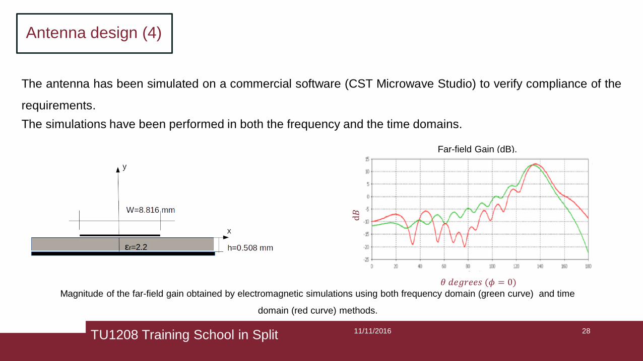
Antenna design (4)
Magnitude of the far-field gain obtained by electromagnetic simulations using both frequency domain (green curve) and time
domain (red curve) methods.
The antenna has been simulated on a commercial software (CST Microwave Studio) to verify compliance of the
requirements.
The simulations have been performed in both the frequency and the time domains.
𝜃 𝑑𝑒𝑔𝑟𝑒𝑒𝑠 (𝜙 = 0)
Far-field Gain (dB).
d𝐵
TU1208 Training School in Split

11/11/2016 29
Simulation domain
In order to verify the penetration depth in the lossy medium, the space gap between the antenna and the
interface has been accurately chosen.
Magnitude of the maximum value of the electric field 𝐸𝑥 (blue line) and
position of the planar interface (green line) .
The interface is located at3
2𝜆 above the microstrip antenna.
The lossy-medium interface intercepts the curve describing
the maxima of the electric field in proximity of 𝑧 = 4𝜆
TU1208 Training School in Split

11/11/2016 30
Deep-penetration evaluation
The magnitude of the electric field, normalized with respect to its value on the interface, inside the lossy material
has been evaluated as a function of the depth.
Simulations have been implemented in three different cases:
• a lossless material, 𝜎2 = 0 S/m
• the lossy material used for the design, 𝜎2 = 0.05S
m
• a lossy material with higher conductivity, 𝜎2 = 0.08 S/m
TU1208 Training School in Split
Field inside the lossy material
11/11/2016 31
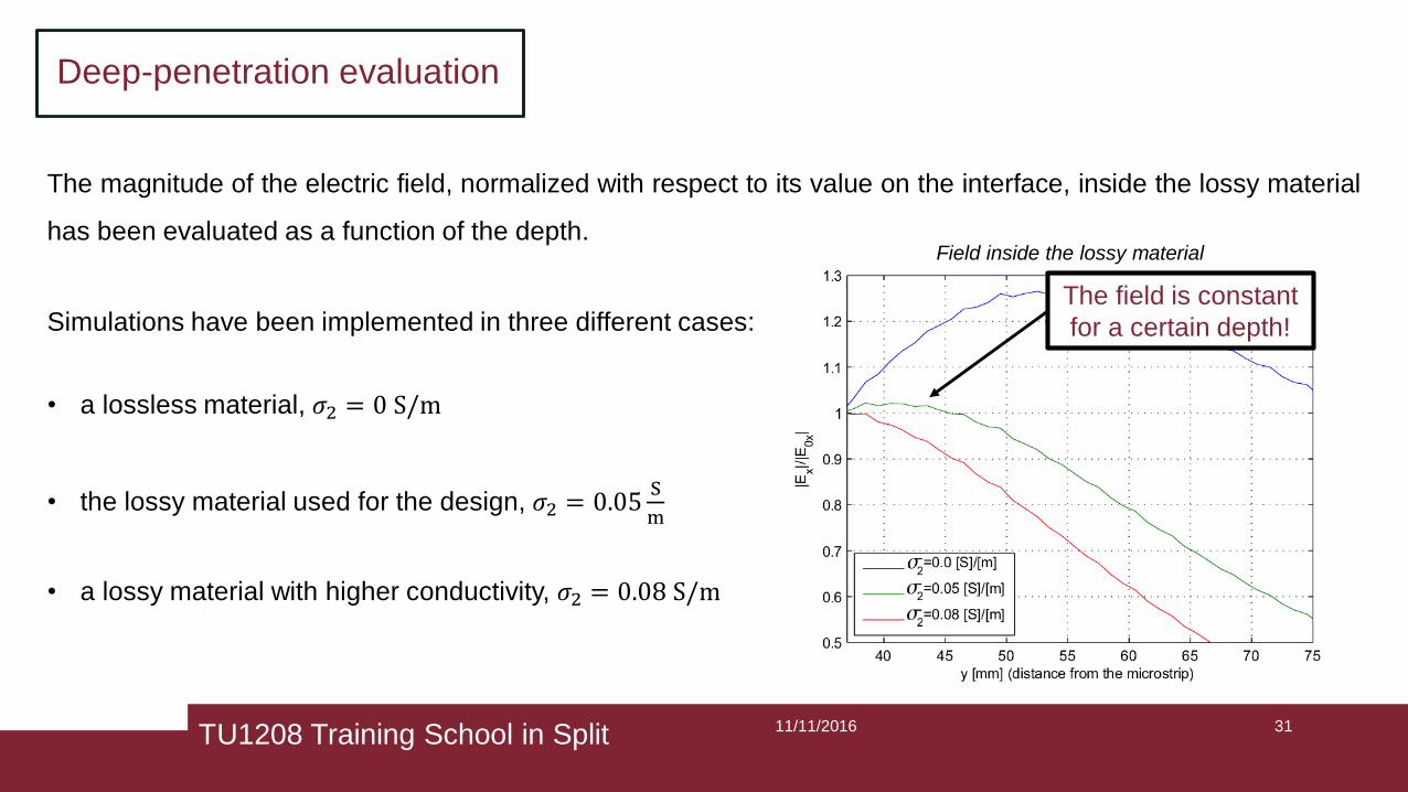
Deep-penetration evaluation
The magnitude of the electric field, normalized with respect to its value on the interface, inside the lossy material
has been evaluated as a function of the depth.
Simulations have been implemented in three different cases:
• a lossless material, 𝜎2 = 0 S/m
• the lossy material used for the design, 𝜎2 = 0.05S
m
• a lossy material with higher conductivity, 𝜎2 = 0.08 S/m
The field is constant
for a certain depth!
TU1208 Training School in Split
Field inside the lossy material

11/11/2016 32
Deep-penetration evaluation (2)
The result presented can be compared with the penetration obtained with a conventional horn antenna
Horn Antenna with lossy mediumLWA and lossy medium
In both cases the lossy medium is placed at 1,5𝜆 from the aperture and its base is parallel to the
antenna aperture.
TU1208 Training School in Split

11/11/2016 33
Deep-penetration evaluation (3)
Horn Antenna parameters.
𝑠11(dB).
d𝐵 d𝐵
𝐹𝑟𝑒𝑞𝑢𝑒𝑛𝑐𝑦 𝐺𝐻𝑧 𝜃 𝑑𝑒𝑔𝑟𝑒𝑒𝑠 (𝜙 = 0)
Farf-ield Gain Abs
The Horn Antenna designed for the comparison presents high gain and it is broadband.
TU1208 Training School in Split

11/11/2016 34
Deep-penetration evaluation (4)
Horn antenna 3D Far-fieldLWA 3D Far-field
3D Far Field comparison between the two antennas.
TU1208 Training School in Split

11/11/2016 35
Deep-penetration evaluation (5)
The result presented for the LWA can be compared with the penetration obtained
with a conventional horn antenna
Mean-Magnitude of the electric field 𝐸𝑥 for a microstrip LWA (left) and a rectangular horn antenna (right)
computed in dB from the generated E-Field
TU1208 Training School in Split

11/11/2016 36
Averaged fields
To allow a fair comparison between different antenna types (and between different LWA longitudinal sections) an
algorithm which would take in consideration mediated fields had to be developed for the LWA.
The electric field produced by the LWA antenna has been mediated on the longitudinal direction 𝑧 on k samples:
The amplitude of the electric field in a point of the lossy medium at a given 𝑧𝑘 is normalized by the mean field
calculated considering all the samples of the Electric field amplitude on the separation surface that precede the
considered point (i.e. for j<k).
𝐸𝐿𝑊𝐴
0, 𝑦𝑖 , 𝑧𝑘 =𝐸𝐿𝑊𝐴 0, 𝑦𝑖 , 𝑧𝑘
𝑗=0𝑗=𝑘−1
𝐸𝑦𝑖𝑓𝐿𝑊𝐴 0, 𝑦𝑖𝑓 , 𝑧𝑗 𝑘
∀𝑦𝑖 > 𝑦𝑖𝑓.
TU1208 Training School in Split

11/11/2016 37
Here we can see the difference between the
actual magnitude of the electric field and the
average magnitude for a given penetration
depth
Averaged fields (2)
TU1208 Training School in Split

11/11/2016 38
Normalized electric field amplitude as a function of the
penetration depth for different longitudinal positions
Deep-penetration comparison
Horizontal line represents the value 1/e
Electric field tends to penetrate more
for higher z values
For z = 80 mm the normalized electric field stays
above 1/e only for 45 mm, but it stays above such a
value for about 80 mm at z = 220 mm
TU1208 Training School in Split
Field inside the lossy material

11/11/2016 39
Averaged global fields (1)
A global mean was also developed. This permitted a penetration “global” mediated comparison between the two
fields.
The electric field produced by the antennas has been mediated on the longitudinal direction 𝑧 on N samples
taken at a distance of 1 mm, N is estimated as the number of samples at the aperture for which the electric field
is reduced by a factor 0.16 of its maximum.
Electric field in a point of the lossy medium is normalized by the mean field calculated considering all the
samples of the Electric field amplitude on the separation surface for which the field is maximum.
E 𝑜, 𝑦𝑖 =Σ𝑘=𝑛𝑘=𝑛+𝑁𝐸 0, 𝑦𝑖 , 𝑧𝑘
𝑗=0𝑗=𝑁
𝐸𝑦𝑖(0, 𝑦𝑖𝑓, 𝑧𝑗)∀𝑦𝑖 > 𝑦𝑖𝑓; yi = yi−1 + 1mm
TU1208 Training School in Split

11/11/2016 40
Averaged global fields (2)
Samples considered for both LWA and Horn
LWA case Horn case
TU1208 Training School in Split

11/11/2016 41
Here we analyze the penetration by considering the
mediated electric field along z
Deep-penetration comparison (2)
The electric field is mediated along 𝑧 on N samples
An algorithm searches the maximum of the electric
field along 𝑧, for each 𝑦. All consecutive samples
with maximum amplitude around this value are
selected until the sum is equal to N
The field generated by the LWA is stronger than the
one generated by the horn for 𝑦 > 80 𝑚𝑚
Horn (𝑠𝑎𝑚𝑝𝑙𝑒𝑠)
Horn (𝑏𝑒𝑠𝑡 𝑓𝑖𝑡)
LWA (𝑠𝑎𝑚𝑝𝑙𝑒𝑠)
LWA (𝑏𝑒𝑠𝑡 𝑓𝑖𝑡)
y [mm]
E𝑜,𝑦𝑖
𝐶𝑜𝑚𝑝𝑎𝑟𝑖𝑠𝑜𝑛 𝑏𝑒𝑡𝑤𝑒𝑒𝑛 𝑎𝑣e𝑟𝑎𝑔𝑒𝑑 𝐻𝑜𝑟𝑛 𝑎𝑛𝑑 𝐿𝑊𝐴𝑝𝑒𝑛𝑒𝑡𝑟𝑎𝑡𝑖𝑜𝑛 in a lossy medium (𝜎 = 0.05 [𝑆]/[𝑚])
TU1208 Training School in Split

11/11/2016 42
• As we seen, a LWA allows to obtain the DPW in a lossy material
• The antenna design can be done with conventional methods
• Comparisons with conventional antennas show a greater amount
of power transmitted in the lossy material
• A strong limitation comes from the value of the phase amplitude
DPW with LWA: conclusions
TU1208 Training School in Split

11/11/2016 43
• As we seen, a LWA allows to obtain the DPW in a lossy material
• The antenna design can be done with conventional methods
• Comparisons with conventional antennas show a greater amount
of power transmitted in the lossy material
• A strong limitation comes from the value of the phase amplitude
DPW with LWA: conclusions
TU1208 Training School in Split
We can wonder if it is possible to generate inhomogeneous waves with alternative mechanisms
11/11/2016 44
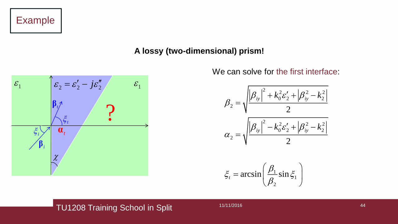
Example
TU1208 Training School in Split
We can solve for the first interface:
22 2 2
0 2 2
2
22 2 2
0 2 2
2
11
2
2
2
arcsin sin
iy iy
iy iy
t
k k
k k
iβ
it
tβ
tα
?
1 2 2 2j 1
A lossy (two-dimensional) prism!

11/11/2016 45
Example (2)
TU1208 Training School in Split
The second interface, a new reference frame:t t
t
22 2 2
0 1 1
3
22 2 2
0 1 1
3
23
3
23
3
2
2
arcsin sin
arcsin sin
ty ty
ty ty
t
t
k k
k k
3 32
t
tβ
tα
3β3α
3

11/11/2016 46
Example (3)
TU1208 Training School in Split
ζ𝟑
χ
β𝟏
ξ𝟏
β𝟐
ξ𝟐 𝜶𝟐
𝜀2 = 𝜀2′ − 𝑗𝜀2
′′𝜀1 𝜀1
β𝟑ξ𝟑
𝜶𝟑
𝜶𝒊𝟐
ζ𝟐𝒊′
ξ𝟐𝒊′
z
y
x
β𝒊𝟐
If a homogeneous wave from a lossless medium impinges on
a dissipative prism (with two non parallel interfaces),
the transmitted wave through the prism is
an inhomogeneous wave in a lossless medium
This can be an alternative approach to obtain inhomogeneous waves
for reach the DPW.
11/11/2016 47
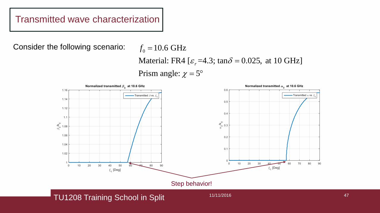
Transmitted wave characterization
TU1208 Training School in Split
Consider the following scenario: 0 10.6 GHz
Material: FR4 [ =4.3; tan 0.025, at 10 GHz]
Prism angle: 5
r
f
Step behavior!
11/11/2016 48
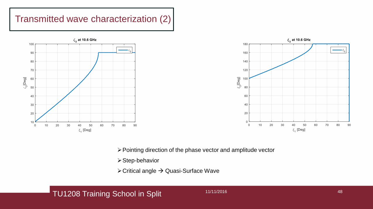
Transmitted wave characterization (2)
TU1208 Training School in Split
Pointing direction of the phase vector and amplitude vector
Step-behavior
Critical angle Quasi-Surface Wave

11/11/2016 49
Lossy-prism antenna
TU1208 Training School in Split
• System composed by the polarizer prism and a field
source.
• The feed of the system is a Ku band rectangular tapered
horn
• Distance between feed and prism:
• 𝑟𝑓𝑓 ≥2𝐷2
𝜆→ 𝑟𝑓𝑓 = 1.0 m
• 𝐿𝑝 takes into account the phase path between phase
center and horn aperture.
• 𝐿𝑚 = 𝑟𝑓𝑓 + 𝐿𝑝
• Prism Side L= sin 𝜃3𝑑𝐵 ∗ (𝐿𝑚 +𝑟𝑓𝑓
2)
• The vertical side is 0.557 m long.

11/11/2016 50
Full-wave analysis
TU1208 Training School in Split
• Ku band rectangular tapered horn
[WR90]
• Lin.Pol.
• Op BW: fc= 10.6 GHz.
• Dmax = 20.1 dB
• θ3𝑑𝐵 = 14.5 deg
• Horn phase centre to provide a
finite section quasi-plane wave
radiated field at the prism interface.

11/11/2016 51
Full-wave analysis (2)
TU1208 Training School in Split
Depointing in line with the theoretical analysis
Defocusing due to prism multiple reflection
Back lobes
CST pattern : tapered horn (green) Vs.system
horn+prism (red).
Electric field along the propagation y-z plane with
dielectric FR4 prism and incidence 𝜉1 =5°.
Frequency 10.6 GHz 10.6 GHz
Directivity peak 20.1 dB 14.8 dB
Pointing Angle 0.0° 3°
𝜽𝟑𝒅𝑩 14.3° 29.2°
SLL -8.3 -3.9

11/11/2016 52
Validation
TU1208 Training School in Split
Very Good Accordance with
theoretical values
TARGET SINGLE HORNHORN+PRISM
(X1I 0°)
HORN+PRISM
(X1I 5°)
HORN+PRISM
(X1I 45°)
MAIN LOBE
MAGNITUDE20.1 DB 14.8 DB 14.4 DB 15.2 DB
MAIN LOBE
DIRECTION0.0° 3° 6° 57°
HPBW 14.3° 29.2° 37.8° 31.1°

11/11/2016 53
A power problem
TU1208 Training School in Split
Up to now, we talked about the wave attenuation in the lossy medium
We considered an incident wave, carrying a certain power,
we considered the transmitted wave, and we found the conditions
under that the transmitted power is not attenuated.
However: how much power can we transmit?
We must consider the reflection coefficient!

11/11/2016 54
Reflection coefficient
TU1208 Training School in Split
We need to maximize the transmitted power
It is possible to transmit the whole incident power?
As it is well known in parallel polarization the total
transmission can be obtained.
However, with lossy materials only a minimum of
the reflection coefficient can be obtained.
The angle of the minimum reflection coefficient is
called Pseudo-Brewster angle

11/11/2016 55
Total Transmission
TU1208 Training School in Split
The expressions of the reflection coefficients:
E-Polarization (s-polarization)
H-Polarization (p-polarization)
If the incident wave is homogeneous, we have a difference between a real and a complex quantity,
It cannot be zero
However, if the incident wave is inhomogeneous, then the reflection coefficient can be zero!
1 2 2 2j

11/11/2016 56
Total Transmission (2)
TU1208 Training School in Split
As it is well known, total transmission can be obtained only in H-polarization
0
Total transmission
condition

11/11/2016 57
Total Transmission (3)
TU1208 Training School in Split
Imposing the dispersion equation, we can obtain the conditions on the properties of the incident wave
Generalized Brewster angle
Brewster phase amplitude

11/11/2016 58
Total Transmission (4)
TU1208 Training School in Split
Reflection coefficient for an interface
between air and gold at λ = 7.7 μm
Reflection coefficient for aninterface between
air and seawater at a frequency of 100MHz

11/11/2016 59
Total Transmission (5)
TU1208 Training School in Split
Two-dimensional maps of the real part of the magnetic field at the interface between a vacuum and medium 2 with relative permittivity ε2.
(a) Medium 2 is lossless, with ε2 = 0.84, the incident wave is homogeneous, and the incident angle is the Brewster angle.
(b) Medium 2 is dissipative, with ε2 = 0.84 + i1.91 (gold at wavelength λ = 7.7 μm), the incident wave is homogeneous, and the incident angle is
the pseudo-Brewster angle.
(c) Medium 2 is dissipative [as in (b)], the incident wave is inhomogeneous with β1 = βB, and the incident angle is the Brewster angle.

11/11/2016 60
Conclusions
• We investigated the fundamental differences between homogeneous and inhomogeneous waves
• The direction of attenuation in a lossy media depends on the nature of the incident wave, if it is
inhomogeneous, the direction of the attenuation can be driven
• Under specific conditions it is possible to make the attenuation parallel to the interface, i.e., to deeply
penetrate the dissipative material
• We presented a practical realization of the DPW through a LWA.
• The comparisons between the penetration depths of the LWA and a canonical Horn antenna have been
shown.
• An alternative approach to obtain the DPW has been proposed through a Lossy-prism antenna
• The possibility to obtain total transmission of the incident power in a lossy medium is still possible if the
incident wave is inhomogeneous
TU1208 Training School in Split
Inhomogeneous waves seem to have several interesting features!